spatio-temporal modelling and probabilistic forecasting of ...€¦ · spatio-temporal modelling...
TRANSCRIPT
Spatio-temporal modelling and probabilisticforecasting of infectious disease counts
Sebastian MeyerInstitute of Medical Informatics, Biometry, and EpidemiologyFriedrich-Alexander-Universität Erlangen-Nürnberg, Erlangen, Germany7 September 2017
Joint work with Johannes Bracher and Leonhard Held (University of Zurich):
Meyer and Held (2017): Incorporating social contact data in spatio-temporal models for infectiousdisease spread. Biostatistics 18:338–351. DOI:10.1093/biostatistics/kxw051
Held, Meyer and Bracher (2017): Probabilistic forecasting in infectious disease epidemiology: the13th Armitage lecture. Statistics in Medicine 36:3443–3460. DOI:10.1002/sim.7363

World Health Organization 2014
Forecasting disease outbreaks is still in its infancy, however, unlikeweather forecasting, where substantial progress has been made inrecent years.
Key requirements to forecast infectious disease incidence
1. Multivariate view to predict incidence in different regions and subgroups
2. Stratified count time series from routine public health surveillance
3. Useful statistical models for such dependent data
4. Suitable measures for the evaluation of probabilistic forecasts
Sebastian Meyer | FAU | Modelling and forecasting epidemics from surveillance counts 7 September 2017 1

Case study: norovirus gastroenteritis in Berlin, 2011–2016— Weekly time series by age group, aggregated over all 12 city districts
25−44 45−64 65+
00−04 05−14 15−24
2012 2013 2014 2015 2016 2012 2013 2014 2015 2016 2012 2013 2014 2015 2016
10
20
30
10
20
30
wee
kly
inci
denc
e [p
er 1
00 0
00 in
habi
tant
s]
[Stratified lab-confirmed counts obtained from survstat.rki.de]
Sebastian Meyer | FAU | Modelling and forecasting epidemics from surveillance counts 7 September 2017 2

Case study: norovirus gastroenteritis in Berlin, 2011–2016— Disease incidence maps by age group, aggregated over time
00−04
0 10 km
chwi frkr
lichmahe
mitt
neuk
pankrein
span
zehl schotrko
196 256 324 400441 484 529 576
05−14
0 10 km
chwi frkr
lichmahe
mitt
neuk
pankrein
span
zehl schotrko
11.5616.00 21.16 27.04 33.64 38.44
15−24
0 10 km
chwi frkr
lichmahe
mitt
neuk
pankrein
span
zehl schotrko
17.6423.04 29.16 36.00 43.56 49.00
25−44
0 10 km
chwi frkr
lichmahe
mitt
neuk
pankrein
span
zehl schotrko
25.00 29.16 33.64 38.44 43.56
45−64
0 10 km
chwi frkr
lichmahe
mitt
neuk
pankrein
span
zehl schotrko
36.00 43.5649.00 54.76 60.84 67.24
65+
0 10 km
chwi frkr
lichmahe
mitt
neuk
pankrein
span
zehl schotrko
144 196 256 289 324 361 400 441
Sebastian Meyer | FAU | Modelling and forecasting epidemics from surveillance counts 7 September 2017 3

Infectious disease spread ~ social contacts
age group of contact
age
grou
p of
par
ticip
ant
00−04
05−09
10−14
15−19
20−24
25−29
30−34
35−39
40−44
45−49
50−54
55−59
60−64
65−69
70+
00−0
4
05−0
9
10−1
4
15−1
9
20−2
4
25−2
9
30−3
4
35−3
9
40−4
4
45−4
9
50−5
4
55−5
9
60−6
4
65−6
970
+0.0
0.5
1.0
1.5
2.0
2.5
3.0
3.5
4.0
aver
age
num
ber
of c
onta
ct p
erso
ns EU-funded POLYMOD study[Mossong et al. 2008]:
• 7 290 participants from eightEuropean countries recordedcontacts during one day
• Contact characteristics weresimilar across countries
• Remarkable mixing patternswith respect to age
Sebastian Meyer | FAU | Modelling and forecasting epidemics from surveillance counts 7 September 2017 4

Starting point for our statistical modelling framework
We have:
• Public health surveillance counts Ygrt indexed by group, region, time period• Social contact matrix C = (cg′g)
• Maybe additional covariates (climate, socio-demographics, . . . )
We would like to model all three data dimensions (g, r , t) and account for theirdependent nature:
g: social mixing patterns between age groups
r : spatial dynamics through human travel
t : temporal dependencies inherent to communicable diseases
Sebastian Meyer | FAU | Modelling and forecasting epidemics from surveillance counts 7 September 2017 5
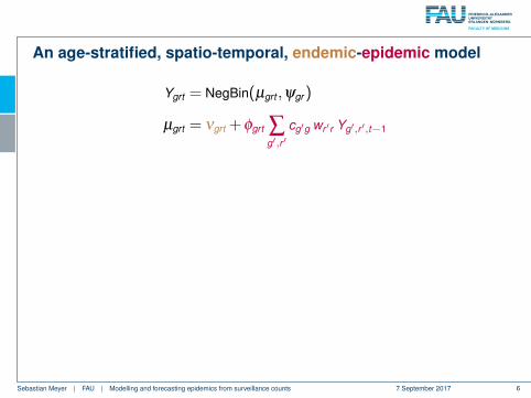
An age-stratified, spatio-temporal, endemic-epidemic model
Ygrt = NegBin(µgrt ,ψgr)
µgrt = νgrt +φgrt ∑g′,r ′
cg′g wr ′r Yg′,r ′,t−1
Contact matrix (cg′g) for g′→ g,aggregated from POLYMOD
age group of contact
age
grou
p of
par
ticip
ant
00−04
05−14
15−24
25−44
45−64
65+
00−04 05−14 15−24 25−44 45−64 65+
0.0
0.1
0.2
0.3
0.4
0.5
Spatial weights for r ′→ r ,power-law decay wr ′r = (or ′r + 1)−ρ
3.0% 8.4%
8.4%3.0%
8.4%
3.0%
46.8%8.4%
3.0%
1.5% 3.0%3.0%
Log-linearpredictors
νgrt and φgrt
• Population
• Seasonality
• Group-specificsusceptibility
• (Covariates)
Sebastian Meyer | FAU | Modelling and forecasting epidemics from surveillance counts 7 September 2017 6

An age-stratified, spatio-temporal, endemic-epidemic model
Ygrt = NegBin(µgrt ,ψgr)
µgrt = νgrt + φgrt ∑g′,r ′
cg′g wr ′r Yg′,r ′,t−1
Contact matrix (cg′g) for g′→ g,aggregated from POLYMOD
age group of contact
age
grou
p of
par
ticip
ant
00−04
05−14
15−24
25−44
45−64
65+
00−04 05−14 15−24 25−44 45−64 65+
0.0
0.1
0.2
0.3
0.4
0.5
Spatial weights for r ′→ r ,power-law decay wr ′r = (or ′r + 1)−ρ
3.0% 8.4%
8.4%3.0%
8.4%
3.0%
46.8%8.4%
3.0%
1.5% 3.0%3.0%
Log-linearpredictors
νgrt and φgrt
• Population
• Seasonality
• Group-specificsusceptibility
• (Covariates)
Sebastian Meyer | FAU | Modelling and forecasting epidemics from surveillance counts 7 September 2017 6

Power-adjustment of the contact matrix: Cκ := EΛκE−1
κ = 0
age group of contact
age
grou
p of
par
ticip
ant
00−04
05−14
15−24
25−44
45−64
65+
00−0405−1415−2425−4445−64 65+
0.0
0.2
0.4
0.6
0.8
1.0
κ = 0.5
age group of contact
age
grou
p of
par
ticip
ant
00−04
05−14
15−24
25−44
45−64
65+
00−0405−1415−2425−4445−64 65+
0.0
0.2
0.4
0.6
0.8
1.0
κ = 1
age group of contact
age
grou
p of
par
ticip
ant
00−04
05−14
15−24
25−44
45−64
65+
00−0405−1415−2425−4445−64 65+
0.0
0.2
0.4
0.6
0.8
1.0
κ = 2
age group of contact
age
grou
p of
par
ticip
ant
00−04
05−14
15−24
25−44
45−64
65+
00−0405−1415−2425−4445−64 65+
0.0
0.2
0.4
0.6
0.8
1.0
Sebastian Meyer | FAU | Modelling and forecasting epidemics from surveillance counts 7 September 2017 7
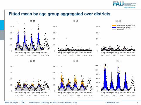
Fitted mean by age group aggregated over districts
0
10
20
30
40
2011 2012 2013 2014 2015 2016
00−04
●
●
●
●●●●●
●
●
●
●
●●
●
●
●
●
●
●
●
●
●
●
●
●
●
●
●
●
●
●●
●
●
●
●
●
●
●●
●●
●
●
●
●
●
●
●
●
●
●
●
●
●
●
●
●
●●●
●
●
●
●
●
●
●
●
●
●
●
●
●
●
●
●
●
●●
●
●
●
●
●
●
●
●
●
●
●
●●●
●
●
●
●
●
●
●
●
●
●
●
●
●
●
●
●
●
●
●
●
●
●●●
●
●
●
●
●
●
●
●
●
●
●
●
●
●
●
●
●
●
●
●
●
●
●
●
●
●
●
●
●
●
●
●●
●
●
●
●
●
●
●
●●
●
●
●
●
●
●
●
●
●
●
●
●
●
●
●
●
●
●
●
●
●
●
●
●
●
●
●
●
●
●
●
●
●
●
●
●
●
●
●
●
●●●●
●
●
●
●
●
●
●
●
●
●
●
●●
●
●
●
●
●
●
●
●●
●
●
●
●
●
●
●
●
●
●
●
●
●
●
●
●
●
●
●
●
●
●
●
●
●
●
●
●
●
●
●
●
●
0
10
20
30
40
2011 2012 2013 2014 2015 2016
05−14
●●
●
●
●●
●
●
●●●●
●
●●
●
●
●
●
●
●●●
●
●●●●
●●
●●
●●
●●
●●
●
●
●
●
●●
●
●●●●
●
●
●●
●●
●●
●
●
●
●●
●
●
●
●
●●●
●
●●
●
●●
●
●
●
●
●
●
●
●●●
●
●●
●
●
●●●
●
●●●●●●
●
●●
●
●
●
●
●
●
●
●●
●
●●●
●●●
●
●
●
●●●●
●
●
●
●
●
●
●
●
●
●
●
●●
●
●●
●●
●●
●●
●
●●
●
●●
●
●
●●●
●
●●
●
●
●
●●
●
●
●●
●
●●
●●
●
●
●
●
●
●
●
●●
●
●
●
●●●●
●
●
●
●●●●●●
●●
●●●●
●●
●
●
●●
●●
●
●
●
●●●
●
●
●
●
●
●●
●
●
●●●
●●
●
●
●
●
●●
●
●
●
●
●●●
●
●●
●
●●
●
●●
●
●● 0
10
20
30
40
2011 2012 2013 2014 2015 2016
15−24
●
●
●
●
●●
●
●
●●
●
●
●
●
●
●
●
●
●
●
●
●
●
●
●
●
●
●●
●
●
●
●
●
●
●
●
●
●
●●
●
●
●
●
●
●
●
●
●●●●●
●
●
●
●
●
●●
●
●
●
●
●
●●
●
●
●
●
●
●
●
●
●
●●
●
●
●
●
●
●●
●
●
●●
●●
●●
●●
●●
●
●
●●●
●●●●
●
●
●
●
●
●
●
●
●
●
●
●
●
●
●
●
●
●
●
●
●
●
●
●
●
●
●
●
●
●
●
●
●
●
●
●●
●●●●●
●
●●
●
●
●●●●●
●●
●●●
●
●
●
●
●●
●●
●
●
●
●
●
●
●
●
●
●●
●
●●
●●
●●
●
●●●●●
●
●●
●
●●●●
●●
●
●
●
●
●
●●
●
●
●
●
●
●
●●●
●●
●
●
●
●
●
●
●
●
●
●●●
●
●
●●●●
●
●
●
●
●
●
●●●
●
●●●●
●
●●
●
from other age groupswithin age groupendemic
0
10
20
30
40
2011 2012 2013 2014 2015 2016
25−44
●
●
●
●
●
●
●
●
●
●●
●
●
●
●
●
●
●
●
●
●
●
●
●
●
●
●
●●
●
●
●
●
●
●
●
●
●
●
●
●
●
●
●
●
●
●
●
●
●
●
●
●
●
●●
●
●●
●
●
●
●
●
●
●
●
●
●
●
●
●
●
●
●
●
●
●
●
●
●
●
●●●
●
●
●
●●
●
●●
●
●
●
●
●
●
●
●
●
●
●●
●
●
●●
●
●
●
●
●
●
●●●
●
●
●
●
●●
●
●
●
●●
●
●
●●
●
●
●
●
●
●
●
●●
●
●
●
●
●
●
●
●
●
●
●
●
●●
●
●
●
●
●
●
●
●●
●
●
●
●
●
●
●
●
●
●
●●
●
●
●
●
●
●
●
●
●
●●
●
●
●
●
●
●
●
●
●
●
●
●
●
●
●
●
●
●
●
●
●
●●
●
●
●●
●
●
●
●
●
●
●
●
●
●
●
●
●
●
●
●
●
●
●
●
●
●
●●
●
●
●
●
●
●●
●
●
●
●
●
●●
●●
●
●
●
●
●
0
10
20
30
40
2011 2012 2013 2014 2015 2016
45−64
●
●
●●●
●
●
●
●
●●
●
●
●
●
●
●
●●
●
●
●
●
●
●
●
●
●
●
●
●
●
●●
●
●
●
●
●
●
●
●
●
●
●
●●
●
●
●
●
●
●
●
●
●
●
●
●
●
●
●
●
●
●
●
●
●
●
●
●
●
●
●
●●
●
●
●
●
●
●
●
●
●
●
●
●●
●
●
●
●
●
●●●●●
●
●
●
●
●
●
●
●
●
●
●
●
●●●
●
●
●
●
●●
●
●
●
●
●
●
●
●
●
●
●
●
●
●
●●
●
●
●
●
●
●
●
●●
●
●●
●
●
●
●
●●
●
●●●
●
●
●
●
●
●
●
●
●●
●
●
●
●
●
●
●
●
●
●
●
●
●
●
●
●
●
●
●●
●
●
●
●
●
●
●
●
●
●
●
●
●
●●
●
●
●
●
●
●
●●
●
●●
●
●
●
●
●●
●
●
●
●
●
●
●
●●
●
●
●●
●
●
●
●
●
●
●●
●
●
●
●●
●
●
●
●
●
●
●
●
●
●
●
●
●
●
0
20
40
60
80
100
120
2011 2012 2013 2014 2015 2016
65+
●●●
●●●●
●●
●
●●●
●
●●●
●
●
●
●
●
●
●
●
●●●
●
●
●
●
●●
●
●
●
●
●
●
●●
●
●
●
●●
●
●
●●●
●●
●●
●●●
●
●
●
●●●●
●
●
●
●
●●
●
●
●
●
●
●●
●
●
●
●●●
●
●●
●
●
●
●
●
●
●●
●
●
●
●
●●
●●
●●
●
●
●
●●●●
●
●
●●
●
●
●
●
●
●●
●
●
●
●
●
●
●
●●
●
●
●
●
●
●
●
●
●
●
●
●
●
●
●●
●●
●●●
●●
●●●●
●
●
●●
●●●●
●
●
●●●
●
●
●
●
●
●
●
●
●
●
●
●
●
●●
●
●
●
●
●●●●
●
●
●
●
●
●
●
●
●
●
●
●
●
●●
●
●
●●●
●
●
●●
●
●●
●●
●
●
●
●
●
●
●
●
●●
●
●
●
●
●●
●
●
●
●
●
●
●
●●●
●
●
●
●
●
●●●●
120
Sebastian Meyer | FAU | Modelling and forecasting epidemics from surveillance counts 7 September 2017 8

Estimated seasonality
0.0
0.5
1.0
1.5
2.0
2.5
3.0
calendar week
ende
mic
sea
sona
lity
(mul
tiplic
ativ
e ef
fect
)
00−0405−1415−2425−4445−6465+
00−04
05−14
15−24
25−44
45−64
65+
27 35 43 51 3 7 11 19
0.0
0.2
0.4
0.6
0.8
1.0
calendar week
epid
emic
pro
port
ion
27 35 43 51 3 7 11 19
Sebastian Meyer | FAU | Modelling and forecasting epidemics from surveillance counts 7 September 2017 9

Spatial power-law weights
0.0
0.2
0.4
0.6
0.8
1.0
adjacency order
wei
ght
0 1 2 3 4
●
●
●● ●
●
●
uniform spatial spreadpower lawunconstrainedlocal transmission only
Power transformation of the contact matrix
κ̂ = 0.41 (95% CI: 0.29 to 0.60)
Sebastian Meyer | FAU | Modelling and forecasting epidemics from surveillance counts 7 September 2017 10
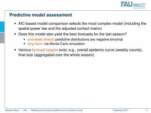
Predictive model assessment
• AIC-based model comparison selects the most complex model (including thespatial power law and the adjusted contact matrix)
• Does this model also yield the best forecasts for the last season?• one-week-ahead: predictive distributions are negative binomial• long-term: via Monte Carlo simulation
• Various forecast targets exist, e.g., overall epidemic curve (weekly counts),final size (aggregated over the whole season)
• “Best” is quantified in terms of sharpness and calibration of the forecasts• Proper scoring rules serve as overall performance measures [Gneiting and
Katzfuss 2014]• Assign penalty score based on the predictive distribution F and the actual
observation yobs• Example: Dawid-Sebastiani score
DSS(F ,yobs) = log|Σ|+(yobs−µ)>Σ−1(yobs−µ)
Sebastian Meyer | FAU | Modelling and forecasting epidemics from surveillance counts 7 September 2017 11
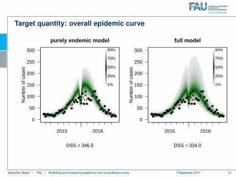
Target quantity: overall epidemic curve
purely endemic model
DSS = 346.5
Num
ber
of c
ases
2015 2016
0
50
100
150
200
250
300
●●
●●●●●
●●
●●
●●●
●●
●
●●
●
●
●
●
●●
●●
●
●
●
●
●
●●●
●
●●
●
●●
●●
●
●
●●
●
●
●●
●●
1%
25%
50%
75%
99%
full model
DSS = 334.0
Num
ber
of c
ases
2015 2016
0
50
100
150
200
250
300
●●
●●●●●
●●
●●
●●●
●●
●
●●
●
●
●
●
●●
●●
●
●
●
●
●
●●●
●
●●
●
●●
●●
●
●
●●
●
●
●●
●●
1%
25%
50%
75%
99%
Sebastian Meyer | FAU | Modelling and forecasting epidemics from surveillance counts 7 September 2017 12

Target quantity: final size by age group
purely endemic model
00−0
4
05−1
4
15−2
4
25−4
4
45−6
465
+
0
500
1000
1500
200025003000
●
●●
●●
●
1%
25%
50%
75%
99%
DSS = 67.9
full model
00−0
4
05−1
4
15−2
4
25−4
4
45−6
465
+
0
500
1000
1500
200025003000
●
●●
●●
●
1%
25%
50%
75%
99%
DSS = 46.5
Sebastian Meyer | FAU | Modelling and forecasting epidemics from surveillance counts 7 September 2017 13

Conclusion
• Models do not perfectly represent individual-level disease transmission, butare still useful for prediction of aggregate-level surveillance counts
• Endemic-epidemic modelling frameworks are implemented in surveillance,also for individual-level data on disease occurrence [Meyer, Held, and Höhle 2017]
• Spatial weights and social contact data improve model fit and predictions• The data and code to reproduce some of the presented results is available in
the supplementary package hhh4contacts [Meyer and Held 2017]
• If the modelling goal is forecasting, use proper scoring rules to assess thequality of probabilistic forecasts [Held, Meyer, and Bracher 2017]
Sebastian Meyer | FAU | Modelling and forecasting epidemics from surveillance counts 7 September 2017 14

References
Gneiting, Tilmann and Katzfuss, Matthias (2014). “Probabilistic forecasting”. In: AnnualReview of Statistics and Its Application 1.1, pp. 125–151. DOI:10.1146/annurev-statistics-062713-085831.
Held, Leonhard, Meyer, Sebastian, and Bracher, Johannes (2017). “Probabilisticforecasting in infectious disease epidemiology: the 13th Armitage lecture”. In: Statisticsin Medicine 36.22, pp. 3443–3460. DOI: 10.1002/sim.7363.
Meyer, Sebastian and Held, Leonhard (2017). “Incorporating social contact data inspatio-temporal models for infectious disease spread”. In: Biostatistics 18.2,pp. 338–351. DOI: 10.1093/biostatistics/kxw051.
Meyer, Sebastian, Held, Leonhard, and Höhle, Michael (2017). “Spatio-temporal analysisof epidemic phenomena using the R package surveillance”. In: Journal of StatisticalSoftware 77.11, pp. 1–55. DOI: 10.18637/jss.v077.i11.
Mossong, Joël et al. (2008). “Social contacts and mixing patterns relevant to the spread ofinfectious diseases”. In: PLoS Medicine 5.3, e74. DOI:10.1371/journal.pmed.0050074.
World Health Organization (2014). “Anticipating epidemics”. In: Weekly EpidemiologicalRecord 89.22, p. 244. URL: http://www.who.int/wer.
Questions? Comments? Z [email protected]

Appendix

Disease incidence map
noroBEr <- noroBE(by = "districts",timeRange=c("2011-w27","2016-w26"))
scalebar <- layout.scalebar(noroBEr@map,corner = c(0.7, 0.9), scale = 10,labels = c(0, "10 km"), cex = 0.6,height = 0.02)
plot(noroBEr, type = observed ~ unit,sub = "Mean yearly incidence",population = rowSums(pop2011) *(nrow(noroBEr)/52)/100000,
labels = list(cex = 0.8),sp.layout = scalebar)
2011/27 − 2016/26
Mean yearly incidence
0 10 km
chwi frkr
lichmahe
mitt
neuk
pankrein
span
zehl schotrko
49.00 64.00 81.0090.25 110.25 132.25 144.00 156.25 169.00
Sebastian Meyer | FAU | Modelling and forecasting epidemics from surveillance counts 7 September 2017 1

Example code for a “simple” version of the model
library("surveillance") # basic "hhh4" modelling frameworklibrary("hhh4contacts") # norovirus and contact data
noroBEall <- noroBE(by = "all", flatten = TRUE, # 6 x 12 = 72 columnstimeRange = c("2011-w27", "2016-w26"))
fit <- hhh4(stsObj = noroBEall, control = list(end = list(f = addSeason2formula(~1),
offset = prop.table(population(noroBEall), 1)),ne = list(f = ~1 + log(pop),
weights = W_powerlaw(maxlag = 5, log = TRUE),scale = expandC(contactmatrix(), 12)),
data = list(pop = prop.table(population(noroBEall), 1)),family = "NegBin1", subset = 2:(4*52)))
Sebastian Meyer | FAU | Modelling and forecasting epidemics from surveillance counts 7 September 2017 2
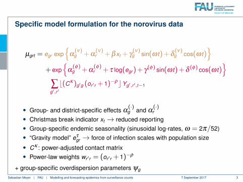
Specific model formulation for the norovirus data
µgrt = egr exp{
α(ν)g +α
(ν)r +β xt + γ
(ν)g sin(ω t)+δ
(ν)g cos(ω t)
}+ exp
{α(φ)g +α
(φ)r + τ log(egr)+ γ
(φ) sin(ω t)+δ(φ) cos(ω t)
}∑g′,r ′b(Cκ)g′g (or ′r + 1)−ρcYg′,r ′,t−1
• Group- and district-specific effects α(·)g and α
(·)r
• Christmas break indicator xt → reduced reporting• Group-specific endemic seasonality (sinusoidal log-rates, ω = 2π/52)• “Gravity model” eτ
gr → force of infection scales with population size• Cκ : power-adjusted contact matrix• Power-law weights wr ′r = (or ′r + 1)−ρ
+ group-specific overdispersion parameters ψg
Sebastian Meyer | FAU | Modelling and forecasting epidemics from surveillance counts 7 September 2017 3