pmr introduction - probabilistic modelling and … introduction probabilistic modelling and...

Welcome Probability Refresher Some Distributions

PMR IntroductionProbabilistic Modelling and Reasoning

Amos Storkey

School of Informatics, University of Edinburgh

Amos Storkey — PMR Introduction School of Informatics, University of Edinburgh 1/50


Outline

1 Welcome

2 Probability Refresher

3 Some Distributions



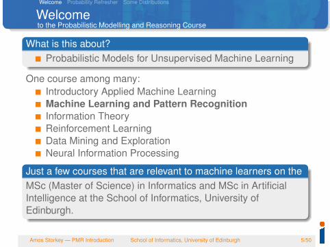
Welcometo the Probabilistic Modelling and Reasoning Course

What is this about?Probabilistic Models for Unsupervised Machine Learning

One course among many:Introductory Applied Machine LearningMachine Learning and Pattern RecognitionInformation TheoryReinforcement LearningData Mining and ExplorationNeural Information Processing

Just a few courses that are relevant to machine learners on theMSc (Master of Science) in Informatics and MSc in ArtificialIntelligence at the School of Informatics, University ofEdinburgh.



Why?

Exciting area of endeavourCoherent.Interesting (and some unsolved...) problems.Now ubiquitous...Relevant to data analytics, business analytics, financial modelling, medical systems, signal

processing, condition monitoring, brain science, the scientific method, image analysis and computer vision,

language modelling, speech modelling, handwriting recognition, risk management, medical imaging, web

analytics, recommender engines, computer games engines, geoinformational systems, intelligent

management, operational research, etc. etc. etc.

In great demand.



What is the Point of Studying this Course?

What should you be able to do after this course?Understand the foundations of Bayesian statistics.Understand why probabilistic models are the appropriatemodels for reasoning with uncertainty.Know how to build structured probabilistic models.Know how to learn and do inference in probabilisticmodels.Know how to apply probabilistic modelling methods inmany domains.



How to succeed

We will use David Barber’s book as our ‘Hitchhikers guideto Probabilistic Modelling’.

Don’t Panic

Hard course. Decide now whether to do it. Then don’t panic.

Work together...

Practice... Use tutorials. Hand in tutorial questions for marking.

Ask me questions. Yes. Even in the lectures. Use the nota bene.

Keep on top. Don’t let it slip.

Do this and I promise you will learn more on this coursethan any other course you have done or are doing!



How to succeed

Working together is critical. Working on your own is criticalfor effective working together.

Tutorials are vital. They are the only way to survive thecourse!Form pairs or small groups within your tutorial.Arrange a meeting a day or two prior to the tutorial to gothrough the tutorial questions together.Try the questions yourself first. Then get together todiscuss. Work out where you are uncertain. Work out whatyou don’t follow. Prepare questions for the tutorial.Use the online nota bene site: Ask questions. Answerothers questions. Minimize the time being stuck andmaximize understanding.Don’t try to rote learn this course. Focus on understanding.



How to succeed

Be boldYou are not supposed to understand everythingimmediately. Its hard! Its supposed to be.Ask, Ask, Ask. Ask yourself. Ask other people. Ask me.Ask in lecturers.Don’t rely on lectures. You need more than lectures.Make lectures better! Prepare beforehand. Ask during.Again use nota bene when you get stuck. Ask a Q. Its okayto just say “I don’t get it. Can you put it a different way.”Work through example questions. Lots of them. If you can’tdo a question you are missing something. Fix it.



Stop point

Quick break.



Probabilistic Machine Learning



Thinking about Data

Probabilistic Modelling does not give us something fornothing.Prior beliefs and model + data→ posterior beliefs.Can do nothing without some a priori model - noconnection between data and question.A priori model sometimes called the inductive bias.



Illusions

Logvinenko illusionInverted mask illusion



Logvinenko Illusion



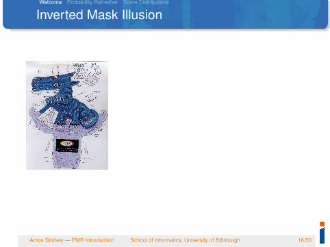
Inverted Mask Illusion



Example: Single Image Super-Resolution

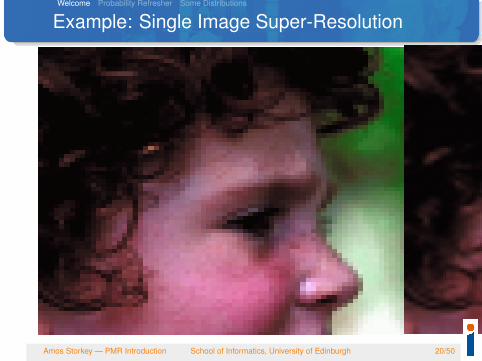
ExampleGiven lots of example images...Learn how to fill in a high resolution image given a singlelow resolution one.State of the art is hard to beat, and appears to be inwidespread use.However state of art technology appears to be restricted toa small region in Los Angeles area.Technology used unknown but seems particularly pertinentat discovering reflections of people in windows, and isusually accompanied by series of short beeps in quickprocession.




Ancknowledgements: Duncan Robson




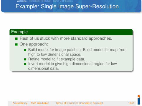
ExampleRest of us stuck with more standard approaches.One approach:

Build model for image patches. Build model for map fromhigh to low dimensional space.Refine model to fit example data.Invert model to give high dimensional region for lowdimensional data.



Reading

Please read David Barber’s book Chapter 1: ProbabilityRefresher.Try some of the exercises at the end.



Probability Introduction

Event Space, Sigma Field, Probability measure.Prior beliefs and model + data→ posterior beliefs.Can do nothing without some a priori model - noconnection between data and question.A priori model sometimes called the inductive bias.



Event Space

The set of all possible future states of affairs is called theevent space or sample space and is denoted by Ω.A σ-field F is a collection of subsets of the event spacewhich includes the empty set ∅, and which is closed undercountable unions and set complements.Intuitively... The event space is all the possibilities as towhat could happen (but only one will). σ-fields are all thebunches of possibilities that we might be collectivelyinterested in.σ-fields are what we define probabilities on.A probability measure maps each element of a σ-field to anumber between 0 and 1 (ensuring consistency).



Random Variables

Random variables assign values to events in a way that isconsistent with the underlying σ-field. (x ≤ x ∈ F) – thebunch of possibilities we might be interested in.We will almost exclusively work with random variables. Weimplicitly assume a standard underlying event space andσ-field for each variable we use.P(x ≤ x) is then the probability that random variable x takesa value less than or equal to x.Don’t worry. Be happy.



Rules of Probability

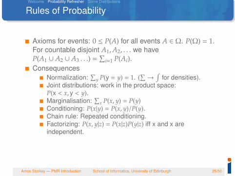
Axioms for events: 0 ≤ P(A) for all events A ∈ Ω. P(Ω) = 1.For countable disjoint A1,A2, . . . we haveP(A1 ∪ A2 ∪ A3 . . .) =

∑i=1 P(Ai).

ConsequencesNormalization:

∑y P(y = y) = 1. (

∑→

∫for densities).

Joint distributions: work in the product space:P(x < x, y < y).Marginalisation:

∑x P(x, y) = P(y)

Conditioning: P(x|y) = P(x, y)/P(y).Chain rule: Repeated conditioning.Factorizing: P(x, y|z) = P(x|z)P(y|z) iff x and x areindependent.



Distribution Functionsof Random Variables

The Cumulative Distribution Function F(x) is F(x) = P(x ≤ x)The Probability Mass Function for a discrete variable isP(x) = P(x = x)The Probability Density Function for a continuous variableis the function P(x) such that

P(x ≤ x) =

∫ x

−∞

P(x = u)du

Think in terms of probability mass per unit length.We will use the term Probability Distribution to informallyrefer to either of the last two: it will be obvious which fromthe context.



Distribution Functionsof Random Variables

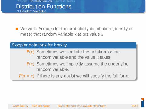
We write P(x = x) for the probability distribution (density ormass) that random variable x takes value x.

Sloppier notations for brevityP(x) Sometimes we conflate the notation for the

random variable and the value it takes.P(x) Sometimes we implicitly assume the underlying

random variable.P(x = x) If there is any doubt we will specify the full form.



Notation

See notation sheet. Notation follows Barber mostly.However I will use capital P for probability, and overload it.Simply put: work out the random variable that P has as anargument, and P makes sense.



Interpretation

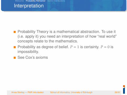
Probability Theory is a mathematical abstraction. To use it(i.e. apply it) you need an interpretation of how “real world”concepts relate to the mathematics.Probability as degree of belief. P = 1 is certainty. P = 0 isimpossibility.See Cox’s axioms



Cox’s Axioms

Assume measure of plausibility f , and map of negation c(.)If

1 Plausibility of proposition implies plausibility of negation:c(c( f )) = f

2 Plausibility of A and B: We can writef (A and B) = g(A,B|A). Then g is associative.

3 Order independence: the plausibility given information isindependent of the order that information arrives in.

Cox’s theorem: plausibility satisfying the above isisomorphic to probability.See also Dutch Book arguments of Ramsey and de Finetti.



Stop point

Quick break.



Distributions

Briefly introduce some useful distributions.Note: Probability mass functions or probability densityfunctions.



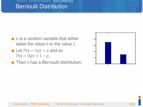
Bernoulli Distribution

x is a random variable that eithertakes the value 0 or the value 1.Let P(x = 1|p) = p and soP(x = 0|p) = 1 − p.Then x has a Bernoulli distribution.

0 10

0.2

0.4

0.6

0.8

1



Multivariate Distribution

x is a random variable that takes oneof the values 1, 2, . . . ,M.Let P(x = i|p) = pi, with

∑mi=1 pi = 1.

Then x has a multivariatedistribution.

1 2 3 40

0.2

0.4

0.6

0.8

1



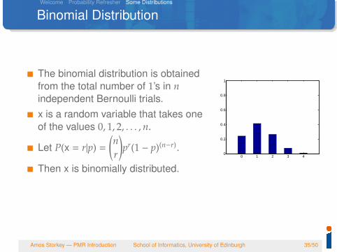
Binomial Distribution

The binomial distribution is obtainedfrom the total number of 1’s in nindependent Bernoulli trials.x is a random variable that takes oneof the values 0, 1, 2, . . . ,n.

Let P(x = r|p) =

(nr

)pr(1 − p)(n−r).

Then x is binomially distributed.0 1 2 3 4

0

0.2

0.4

0.6

0.8

1



Multinomial Distribution

The multinomial distribution is obtained from the total countfor each outcome in n independent multivariate trials withm possible outcomes.x is a random vector of length m taking values x withxi ∈ Z

+ (non-negative integers) and∑m

i=1 xi = n.Let

P(x = x|p) =n!

x1! . . . xm!px1

1 . . . pxmm

Then x is multinomially distributed.



Poisson Distribution

The Poisson distribution is obtainedfrom binomial distribution in the limitn→∞ with p/n = λ.x is a random variable takingnon-negative integer values0, 1, 2, . . ..Let

P(x = x|λ) =λx exp(−λ)

x!

Then x is Poisson distributed.

0 5 10 150

0.05

0.1

0.15

0.2

0.25

0.3

0.35

0.4



Uniform Distribution

x is a random variable taking valuesx ∈ [a, b].Let P(x = x) = 1/[b − a]Then x is uniformly distributed.

NoteCannot have a uniform distribution on anunbounded region.

0 2 4 6 8 100

0.2

0.4

0.6

0.8

1



Gaussian Distribution

x is a random variable taking valuesx ∈ R (real values).Let P(x = x|µ, σ2) =

1√

2πσ2exp

(−

(x − µ)2

2σ2

)Then x is Gaussian distributed withmean µ and variance σ2.

−5 0 5 10 150

0.05

0.1

0.15

0.2

0.25



Gamma Distribution

The Gamma distribution has a rateparameter β > 0 (or a scaleparameter 1/β) and a shapeparameter α > 0.x is a random variable taking valuesx ∈ R+ (non-negative real values).Let

P(x = x|λ) =1

Γ(α)xα−1βα exp(−βx)

Then x is Gamma distributed.Note the Gamma function.

0 2 4 6 8 10 120

0.05

0.1

0.15

0.2

0.25

0.3

0.35



Exponential Distribution

The exponential distribution is aGamma distribution with α = 1.The exponential distribution is oftenused for arrival times.x is a random variable taking valuesx ∈ R+ .Let P(x = x|λ) = λ exp(−λx)Then x is exponentially distributed.

0 5 10 150

0.1

0.2

0.3

0.4

0.5



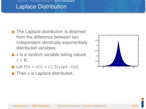
Laplace Distribution

The Laplace distribution is obtainedfrom the difference between twoindependent identically exponentiallydistributed variables.x is a random variable taking valuesx ∈ R.Let P(x = x|λ) = (λ/2) exp(−λ|x|)Then x is Laplace distributed.

−10 −5 0 5 100

0.05

0.1

0.15

0.2

0.25



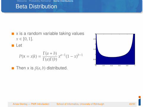
Beta Distribution

x is a random variable taking valuesx ∈ [0, 1].Let

P(x = x|k) =Γ(a + b)Γ(a)Γ(b)

xa−1(1 − x)b−1

Then x is β(a, b) distributed.0 0.2 0.4 0.6 0.8 1

0

0.5

1

1.5

2

2.5

3



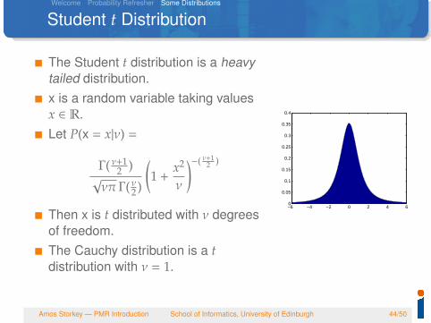
Student t Distribution

The Student t distribution is a heavytailed distribution.x is a random variable taking valuesx ∈ R.Let P(x = x|ν) =

Γ( ν+12 )

√νπΓ( ν2 )

(1 +

x2

ν

)−( ν+12 )

Then x is t distributed with ν degreesof freedom.The Cauchy distribution is a tdistribution with ν = 1.

−6 −4 −2 0 2 4 60

0.05

0.1

0.15

0.2

0.25

0.3

0.35

0.4



The Kronecker Delta

Think of a discrete distribution with all its probability masson one value. So P(x = i) = 1 iff (if and only if) i = j.We can write this using the Kronecker Delta:

P(x = i) = δi j

δi j = 1 iff i = j and is zero otherwise.



The Dirac Delta

Think of a real valued distribution with all its probabilitydensity on one value.There is an infinite density peak at one point (lets call thispoint a).We can write this using the Dirac delta:

P(x = x) = δ(x − a)

which has the properties δ(x − a) = 0 if x , a, δ(x − a) = ∞ ifx = a,∫

∞

−∞

dx δ(x − a) = 1 and∫∞

−∞

dx f (x)δ(x − a) = f (a).

You could think of it as a Gaussian distribution in the limitof zero variance.



Other Distributions

Chi-squared distribution with k degrees of freedom is aGamma distribution with β = 1/2 and k = 2/α.Dirichlet distribution: will be used on this course.Weibull distribution (a generalisation of the exponential)Geometric distributionNegative binomial distribution.Wishart distribution (a distribution over matrices).distributions.Use Wikipedia and Mathworld. Good summaries fordistributions.



Things you must never (ever) forget

Probabilities must be between 0 and 1 (though probabilitydensities can be greater than 1).Distributions must sum (or integrate) to 1.Probabilities must be between 0 and 1 (though probabilitydensities can be greater than 1).Distributions must sum (or integrate) to 1.Probabilities must be between 0 and 1 (though probabilitydensities can be greater than 1).Distributions must sum (or integrate) to 1.Note probability densities can be greater than 1.



Summary

I plan to challenge you.This is going to be hard. Keep up.Theoretical grounding is key.



To Do

Attending lectures is no substitute for working through thematerial! Lectures will motivate the methods and approaches.Only by study of the notes and bookwork will the details beclear. If you do not understand the notes then discuss themwith one another. Ask your tutors.

ReadingThese lecture slides. Chapter 1 of Barber.

Preparatory ReadingBarber Chapter 2.

Extra ReadingCox’s Axioms. Subjective Probability.


pmr introduction - probabilistic modelling and … introduction probabilistic modelling and...

Documents