principal component analysis of potential energy surfaces of large

11/8/09 2:31 PMPrincipal component analysis of potential energy surfaces of large clusters: al..... (DOI: 10.1039/b913802a)

of 16http://www.rsc.org.proxy.uchicago.edu/delivery/_ArticleLinking/Artic…?JournalCode=CP&Year=2009&ManuscriptID=b913802a&Iss=Advance_Article

Journals Physical Chemistry Chemical Physics Advance Articles DOI: 10.1039/b913802a

Phys. Chem. Chem. Phys., 2009 DOI: 10.1039/b913802a Paper

Physical Chemistry Chemical Physics

Principal component analysis of potential energy surfaces of largeclusters: allowing the practical calculation of the master equationNima Shariat Panahi and R. S. Berry * The University of Chicago, 929 East 57th St., Chicago, Illinois 60637, USA. E-mail: [email protected]

Received 10th July 2009 , Accepted 2nd October 2009

First published on the web 6th November 2009

The number of variables in many-particle systems is typically unmanageably large; some way to reducethat number and still retain access to the important information about the system of interest is one of thegreat challenges in the broad topic of complexity. Principal components and principal coordinates providea powerful means to extract—from unwieldy, large data sets—a reduced collection of variables thatprovide the information one needs, in a relatively efficient way and useful form. We investigate theapplication of principal components to the analysis of kinetics of the atomic motions in atomic clusters,particularly of clusters that are large enough so that a full description in terms of the entire high-dimensional potential surface is entirely impractical. A specific application is the use of principalcomponents linking minima with their adjacent saddles, permitting the evaluation of rate coefficients (inthe context of transition state theory) as ratios of partition functions of only one or two key variables.

1 Introduction

1.1 PCO and PCA

The analysis of the potential energy surfaces (PES) of clusters has proven to be a useful tool in theoreticalchemical physics,1–4 especially for relating the interparticle forces to the dynamical and kinetic behaviorof moderately complex systems. With current computational power and efficient algorithms, one can findall of the minima and the important saddles on a potential energy surface for systems composed of up toabout 18 particles. However, the number of geometrically distinct minima grows at least exponentiallywith the number of particles in the system, and the number of saddles grows even faster than that.5 Andthis does not yet take account of the number of permutational isomers. Consequently, cataloging all theminima and important saddles is, at very least, undesirable for 20 particles and more. Even if one were todo such an exhaustive search, most of the topographical information would be of negligible use for theanalysis of dynamics.3 It is thus more desirable—and, in effect, necessary—to reduce drastically thenumber of variables one uses to describe the system. It is clearly desirable to construct a sample PESfrom a statistical sampling of the full PES, but to do this in a way that yields a reasonably accuraterepresentation of the dynamics or kinetics.6 Such a statistical sample PES would, one hopes, be adequate,especially to reveal the most important, and, presumably, slow relaxation processes and their rates. In thispaper, we explore one approach that may offer a means to achieve such a reduction, namely the use ofprincipal component analysis (PCA) and its complement, principal coordinate analysis (PCO);specifically, we examine the use of these tools to evaluate the rate coefficients on a many-dimensionalpotential surface. We use these to avoid having to use the full set of coordinates to find the partitionfunctions and rate coefficients for passages between local potential minima on complex surfaces. In the

http://www.rsc.org.proxy.uchicago.edu/Publishing/Journals/Index.asp

http://www.rsc.org.proxy.uchicago.edu/Publishing/Journals/CP/Index.asp

http://www.rsc.org.proxy.uchicago.edu/Publishing/Journals/CP/Article.asp?Type=AdvArticle

http://www.rsc.org.proxy.uchicago.edu/delivery/_ArticleLinking/ArticleLinking.cfm?JournalCode=CP&Year=2009&ManuscriptID=b913802a&Iss=Advance_Article#fn1

mailto:[email protected]

http://www.rsc.org.proxy.uchicago.edu/delivery/_ArticleLinking/ArticleLinking.cfm?JournalCode=CP&Year=2009&ManuscriptID=b913802a&Iss=Advance_Article#cit1






end, we are able to estimate the minimum size of systems for which this approach would be a significantaid.

This investigation is an exploration of the possibility and potential difficulties in using PCA and PCOto reduce, in one particular way, the unmanageable complexity of the full master equation of a many-body system. Here, we do not address the sampling problem—the choice of criteria for constructing asuitable statistical sample of the full energy landscape. Nor do we address the related problem ofidentifying pathological landscapes, such as those of Ar38, Ar75 or perhaps prions—landscapes withdeep, narrow minima that have energies significantly lower than the readily accessible minima in largebasins, and that typically have structures different from those in the large basins, the landscapessometimes called Stillinger nightmares , after that researcher s conjecture of the existence of suchphenomena.

The methods of sampling pathways on complex potential surfaces have been studied extensivelyelsewhere.6–8 Our focus here is primarily on making more efficient the evaluation of the many ratecoefficients for well-to-well passages. In our study, we chose as our main vehicle an Ar13 cluster,approximated by pairwise Lennard-Jones potentials. We also examined Ar20 for some investigations, toget some sense of the difficulties of working with larger systems. For the 13-atom cluster, a sizemanageable for a relatively detailed study, we began with the database of 1505 geometrically distinctminima and 25 653 important saddles.4,9,10 We selected 100 minima and the 1111 saddles connectingthem as our sample PES. This was done by starting at the global minima and following the connectivitythrough saddles and branching out until we had reached our required 100 minima. We were careful toinclude the most connected minima and branch out from them to other well connected minima so that weobtained a good representation of the connectivity, in order to model the dynamics. In addition, we tookcare to include all transition states directly linking any two minima. The pathways were consistent withthe rough trajectory criterion found previously to be the most successful guide for finding reasonablygood estimates of the slowest rates of motion on the landscape.6

Once the sample PES has been obtained, then the rate constants for well-to-well passage of the argoncluster can be calculated from the topography of the sample PES. We then went on to calculate the masterequation and other important features of the sample PES. Since principal component analysis (PCA) andprincipal coordinate analysis (PCO) offer ways to reduce the dimensionality of the problem in calculatingrate constants and in visualizing the PES, respectively, PCA and PCO can, in principle, be used tocalculate rate constants efficiently and portray the significant features of the PES for large clusters.Specifically, degrees of freedom that do not change significantly from the initial minimum to the saddlecan be neglected in evaluating the rate constant for that transition, within the formalism of transition statetheory, because the partition functions for such degrees of freedom are the same at both places on thepotential surface.

Principal coordinate analysis was first developed by Gower in 1966.11 Gower also showed the dualityof principal coordinate analysis and principal component analysis. PCO is a variant or dual of PCA andboth are means to select the most important out of the whole set of degrees of freedom.11,12

In our work, both PCO and PCA were used. Although there is a duality between the two methods, thetwo are suited for different tasks. For example, PCO is principally suited for visualizing purposes anddoes not provide analytic results.12 On the other hand, PCA is not well suited for reducing thedimensionality of a PES representation but does provide analytic results for the reduced dimensions,12

such as those needed for calculating rate constants. Here, we make quantitative use of PCA, and applyPCO primarily for building an intuitive picture of what the approximating approach is doing.

In this project, first, PCO is used to reduce the dimensionality of the PES of Ar20 in order to representits essentials visually in three-dimensional space. Then, PCA is applied to the Ar13 cluster in order toreduce the vibrational analysis to a set of reduced dimensionality, in order to obtain rate constants fortransitions between minima (using their connecting saddles) in the context of transition state theory. Thatway, when we obtain the rate constants, it becomes simple to construct and solve the master equation.

The crux of this approach is the way the rate coefficient for passage over a barrier is represented as theratio of the partition functions of the transition state and the initial state. These partition functions are










products of the partition functions of the vibrational degrees of freedom. Any degree of freedom that isessentially the same in the initial and transition state contributes the same partition function to thenumerator and denominator of the ratio, and hence, since these cancel, contributes only a factor of unityto the rate coefficient. Only those degrees of freedom that differ significantly in passage from initial totransition state contribute to the rate coefficient. These are precisely the degrees of freedom that PCO andPCA identify.

1.2 Master equation

The stochastic master equation13 dynamics method has previously been applied to the study of thekinetics on a PES13–16 Two general methods have been widely used to study near-equilibrium dynamicsand thermodynamics, such as relaxations of argon clusters: stochastic master equations and moleculardynamics simulations (MD). The stochastic master equation does not reveal the atomic-level detail ofMD, but that method has several advantages over MD. First, solving the master equation is much fasterthan solving the MD equations for the time intervals and time resolutions needed to reach equilibriumand achieve results comparable to master equation solutions. The time-consuming part of solving themaster equation is constructing the transfer matrix (which contains the rate constants between minima)and diagonalizing the resulting N × N matrix (where N is the number of minima in the sample PES). Thisprocess yields the eigenvalues and eigenvectors that solve the equations.14,16,17 The complexity ofdiagonalizing such a matrix is O(N3).

Second, by the method of master equation, we obtain average behavior of an ensemble, whereas MDsimulations require many runs to obtain satisfactory averages.4,18,19,20

Third, aside from the limitations of diagonalizing possibly a large matrix (though in this study, the sizeis limited by choosing a sample PES that is as small as possible in order to describe the dynamics of thecluster and still retain the desired accuracy), the master equation method does not suffer the limitations ofMD, such as large storage requirements, limited total simulation time, and establishing a time scale onwhich ergodicity is achieved in a simulation.

Fourth, the transfer matrix is a product of the theory, in this case Rice-Ramsperger-Kassel-Marcus(RRKM) transition state theory, used to describe the state-to-state kinetics,21,22 and also it retains thecharacteristics of topography of the underlying PES, such as connectivity and energies of the stationarypoints. This allows us to study the effect of different underlying approaches to setting up and solving themaster equation.23

Fifth, the master equation avoids the round-off error propagated in integrating the equations of motionby the MD algorithms. Finally, to obtain kinetic results for different temperatures, new ensembles of MDtrajectories must be calculated, whereas for the master equation, the transition matrix can just be modifiedin a fast and simple manner to account for the temperature dependences of the rate coefficients.

Hence, this is an exploration into a possible way to make manageable the description of the motions ofmoderately complex systems by constructing and solving master equations based on suitably chosensamples of their energy landscapes, as an alternative to using more detailed methods such as moleculardynamics. It is not in any way a study of how to construct the statistical sample, only of examining a waythat may be useful for evaluating the rate coefficients on that sample landscape.

For the Ar13 system, the transition matrix was calculated for a temperature equivalent in Lennard-Jones units to a conventional temperature of 30 K in this work. This temperature was an arbitrary choicethat falls in the range of solid–liquid coexistence for this system. Other temperatures would certainlyinvolve different rates and different equilibrium population distributions. A primary motivation for thiseffort is to try to find a way to speed up and simplify the calculation of the rate constants that comprisethe transition matrix of the master equation. The rate coefficients that are the elements of that matrix are,within the context of transition state theory, ratios of partition functions, at saddles and at the initial statesleading to those saddles. The goal of this effort was to see whether reducing the number of variablesneeded to compute the partition coefficients to just those that carry significant changes, i.e. the mostimportant PCAs and PCOs, would simplify the construction of the master equation to a useful extent.









2 Theory

2.1 Calculating PCO and PCA

PCA is the first step in PCO, as both are duals of each other. PCA uses a correlation matrix formed fromcomparison between variables that set apart one data point from the others. Here, the coordinates are usedas variables and different configurations as individual data points.

We start with an n × p matrix, Y, with n observables and p variables for each observable; here, the twomethods diverge. For PCA, we start with the p × p matrix YTY, measuring the variance between variables.In contrast, PCO uses the n × n matrix YYT, measuring the similarity between configurations. Both PCAand PCO together are the tools of a general method, far more than just our specialized application andexhibit great variety, not only in the fields in which they are applied, but also in how they aremathematically adapted to the need. For example, the distance matrix in PCO can be defined in manyways to obtain what one considers the correct measure of distance (or dissimilarity) for the application.Likewise, PCA s covariance matrix can be replaced with similar matrices, such as correlation or sums-of-squares-cross-products (SSCP),24 depending on the application.

The first step in our use of PCO is setting up the distance matrix between configurations. The matrix is

defined by , where i and j are the configuration indices, r is the coordinate index, X areCartesian coordinates, and dij is the measure of dissimilarity between the ith and jth configurations. Thisdescribes the distance between configurations and is thus suitable for constructing the PES graph.

The second step is constructing a centralized distance matrix as follows:1. Form the A matrix, −dij/2, of interparticle distances.2. Centralize the A matrix and, from it, form the B matrix, bij = aij − ai . − aj . + a.., where ai . is the

average over the ith row, aj . is the average over the jth column, and a.. is the average over the wholematrix A. We do this to remove averages from the calculations and results.

3. Diagonalize the B matrix and obtain the eigenvalues and eigenvectors.4. Normalize the eigenvectors to eigenvalues. That is, normalize the eigenvectors so that their norms

are the corresponding eigenvalues. This is done by dividing the eigenvectors by the square root of thecorresponding eigenvalue.

5. The normalized eigenvalues give the percent of the total variance between the structures containedin the corresponding eigenvector.

We then proceed to pick the first few eigenvectors (or PCOs) with the largest eigenvalues which revealthat they are the ones with the largest variances contained in them, in order to derive the new data set. Toconstruct a 3D graph, we pick the first two eigenvectors and plot the energy as a function of thesevariables, to get a picture of the main features of the PES.

The procedure for PCA is similar to that of PCO:12,25

1. One first subtracts the mean from the data, similar to centralizing our data for the PCO. That is, wesubtract the average across each dimension from each datum in that dimension.

2. We calculate the covariance matrix (see ref. 25 and 26 as needed).3. We then diagonalize the covariance matrix and obtain the eigenvectors and eigenvalues.4. The eigenvectors give a linear combination of the data set. We have done this in two ways. In our

first case, we chose the interatomic distances as the variables and configurations as the data points. In oursecond case, the 3N atomic coordinates are the variables and the configurations are the data points.

5. The normalized eigenvalues give the percentage variance contained in the correspondingeigenvectors.

6. Last, we pick out the most important variables, corresponding to the eigenvectors with the highesteigenvalues, using the linear combination as a weight.

In the central effort of this study, only one eigenvector was picked for the case based on interatomicdistances, and three eigenvectors were picked for the atomic coordinates case. The calculations were also






done with more eigenvectors or PCAs, but this did not change the results, as the mathematics dictatesexactly how many PCA coordinates we need (i.e. the 1-dimensional nature of the interatomic caserequires one PCA while the 3-dimensional nature of the atomic coordinates requires three PCAs). Thisshows that the first few PCAs effectively contain all of the important variance in our data. In the linearcombination, we proceeded to pick the most important interatomic distances by looking at their weights.

This reduction, in turn, told us what coordinates needed to be included in the computation of thereduced Hessian from which we obtained the frequencies required to compute the rate constants of themaster equation. Finally, for the PCO and PCA methods, since we only needed the first few largesteigenvalues/eigenvectors, we used Lanczos methods27 to cut down on computational cost. Thecomputational cost saved by Lanczos method is significant, especially for large systems for which neitherthe computation time nor resources exist to deal with diagonalizing very large matrices. Our own testsshowed that for very large systems, the Lanczos method can be orders of magnitude faster than a fulldiagonalization.

2.2 Constructing the master equation

The stochastic master equation formalism is an initial value problem whose solutions are time-dependentoccupation probabilities for the minima in our sample PES.13 The main component of the master equationis its transition matrix. The eigenvalues and eigenvectors of the transition matrix solve the masterequation. The eigenvalues give the exponential rates of flow of the population distributions on the PES,and the eigenvectors describe these flows in terms of changes in the populations among the minimaconnected to the particular minimum. That is, the absolute value of the jth component of the itheigenvector will determine the magnitude of the rate by which the mode j will change the population atstate i and its sign will determine if the population will increase or decrease.

The first step in constructing the master equation for our system is obtaining the partition functionsused in calculating the rate constants of the RRKM transition state theory. Realistic partition functions,including anharmonic corrections, have been studied in detail elsewhere.23 For our purposes, it sufficesfor us to use a classical harmonic model to obtain the vibrational partition function:

where m is the number of vibrational degrees of freedom in each type of configuration, with m = 3N − 6

= 33 for minima and m = 3N − 7 = 32 for transition states, for kB, the Boltzmann constant, and Tis the temperature (30 K in these calculations), and vj is the jth normal mode vibrational frequency. Thefrequencies, vj, are obtained by diagonalizing the Hessian of a given stationary point. It is here that weuse PCA to dramatically reduce the dimension of the Hessian matrix and thus speed up obtaining thefrequencies. The rationale behind this is that the important quantities, in our case the rate constants andequilibrium solutions to the master equation, use the ratio of vibrational partition functions of theminimum and the saddle. This means that the partition function factors of similar normal modeseffectively cancel out, leaving us with only those normal modes that change between the saddle and theminimum. We can then construct the partition function23

Zi = nsZvibexp(− Vi)

where Vi is the potential energy at the stationary point. The degeneracy factor, ns, accounts for the numberof distinct permutational isomers, and is given by







where np is the total number of nuclear permutations, and hs is the order of the point group for thatconfiguration.28

Transition matrix and master equation. The transition probabilities, Wij, which make up the elementsof the transition matrix, W, for passage from well j to well i (i j) is the sum of the RRKM transitionrates for each of the N ij transition states, l, connecting the wells:

where Vl = Vl − Vj is the barrier height of the transition (Vl and Vj are the potential energies of thetransition state l and minimum j, respectively). Zj and Zl are the partition functions for the local minimumj and the transition state l, respectively. Note that the above equation for Wij is only used to obtain off-diagonal terms in the transition matrix. So, in order to write the master equation in matrix form, we needto define the diagonal terms. The diagonal terms are the combined rates for all transitions out of well iinto wells connected to it:

Now we construct the master equation for the time-dependent probability vector, P(t) [with N (thenumber of minima in the sample PES) components with values Pi(t), the probability of the systemresiding in well i at time t]; writing it in component form:

or writing it in matrix form:

P(t) = WP(t).

The transition matrix, and thus the master equation, do not contain degenerate contributions; that is,transitions to the same well or permutational isomers do not affect the ensemble population of thatgeometry, and therefore are not counted.

The equilibrium, i.e. infinite time, solutions to the master equation are quite simple and are given bythe Boltzmann distribution23

Again, Zi is the partition function for the minimum i, and Vi is the potential energy at that minimum.

Solutions to the master equation. In our calculations, we used a Householder reduction to obtain aQR decomposition and thus diagonalize the transition matrix W.29,30 To use this, and to ensure aspanning set of eigenvectors with real eigenvalues, we need to symmetrize the transition matrix. We canobtain this by evoking the condition of detailed balance:







We therefore form a new symmetric matrix, :

and W have the same eigenvalues, i. Their eigenvectors, and u(i), respectively, are related by

. The final solution to the master equation in terms of the eigenvectors of is:

or in terms of the eigenvectors of W:

In our work, we look at and compare the eigenvalue spectrum and ultimately the relaxation curves Pi(t),which are the solutions to the master equation, to judge the validity of our method. However, also usingeigenvector similarities have been studied elsewhere by Lu et al.6

3 Results

First, we examine the way PCO can give insights into the topography of a complex energy landscape. Forthis, we used the Ar20 cluster, one whose potential is far too complex to be envisioned in any relativelyfull way. We chose 75 points on the PES of Ar20 using the program OPTIM2 by David Wales, with theLennard-Jones potential. Since we were interested in seeing how to apply PCO, and were not concernedhere with finding good methods to choose the PES points to which we would apply PCO, we simplypicked our 75 by starting from the global minimum and the second lowest minimum we could find andbranched out from them by constructing monotonic sequences, but in random directions. We also added afew points just randomly from general non-monotonic sequences originating from the global minimumpoint to complete the picture. We then performed PCO with Cartesian coordinates and picked the mostimportant two eigenvectors to obtain the graph of the PES (Fig. 1).


http://www.rsc.org.proxy.uchicago.edu/delivery/_ArticleLinking/ArticleLinking.cfm?JournalCode=CP&Year=2009&ManuscriptID=b913802a&Iss=Advance_Article#fig1



Fig. 1 Principal coordinate representation of the PES of Ar20 based on the two most importantprincipal coordinates derived from the Cartesian coordinates of the particles.

We can see that the PES of Ar20 has two main funnels, at least in the portion we sampled. Thus, withonly two PCO eigenvectors, we were able to get a good picture of the complex PES of Ar20. Becausealmost all the variance between these two stable forms is encapsulated in the two principal coordinates,they are adequate for estimating the effective distance between them.

Then we turned to the more quantitative problem of finding whether PCA can be used to reduce thedimensionality of the problem of finding rate coefficients. For Ar13, we applied PCA. First, we formedthe data with interatomic distances as the variables (N(N − 1)/2 of them) and stationary points asconfigurations. We then performed PCA and picked the first eigenvector. Out of the first eigenvector, wepicked the highest weights corresponding to the most important interatomic distances. For all rateconstants, the first eigenvector effectively represented all the variance of the data. With those data, wethen proceeded to do harmonic vibrational analysis using the Hessian matrix on the minima and saddles.Finally, we constructed and solved the master equation to get the eigenvalues. We repeated thecalculation a second time with the modification of using atomic coordinates as the variables (3N of them)and stationary points as configurations and taking the three largest eigenvectors instead of one. Wecompared the eigenvalue spectra obtained from a full Hessian and from our two-PCA reduced Hessian(Fig. 2 and 3).




Fig. 2 The eigenvalue spectra of the full master equationcompared with PCA using interatomic distances.

Fig. 3 The eigenvalue spectra of the full master equationcompared with PCA using atomic coordinates.

As we can see from the spectral graphs, the PCAs give results for the eigenvalue spectrum nearlyidentical with those of the full treatment. However, the relaxation curves are an even better match thanthe spectra, as discussed below. Also, the PCA, using two principal components for interatomic distances,gave exactly the same spectrum as that from PCA with one component since, as stated above, the secondPCA adds nothing to the variance (that is, the first PCA component represented 100% of the motionswith the remaining components adding nothing, due to the fact that changes in the cluster are completelycaptured by the change in the bonds, which are 1-dimensional and thus the largest covariance eigenvectorcontains all the variance). A similar thing happened with more than three principal components based onthe atomic coordinates for the reasons states above. For this case of three principal components, thevariance divided between the three components varied from case to case, but the variance dividedsomewhat equally on average among the three; each contained about 1/3 of the variance. This behavior ofthe coordinate-based PCAs meant that in this representation, one must keep three components, sinceeliminating any of them would mean losing roughly 1/3 of the variance. Adding more than threecomponents increased computations dramatically but added nothing. However, these three componentsgave us the same PCA spectrum as that based on interatomic distances, but with a much improved speedin computation compared to the interatomic method. Finally, it is very important to note that the similaritybetween the full master equation and one based on PCA reduced coordinates is especially strong for thehighest (least negative) eigenvalues, which dominate the relaxation process. We see the numericalcomparison for eigenvalues listed from highest to lowest (log nearest zero and hence slowest process


of 16http://www.rsc.org.proxy.uchicago.edu/delivery/_ArticleLinking/Arti…?JournalCode=CP&Year=2009&ManuscriptID=b913802a&Iss=Advance_Article

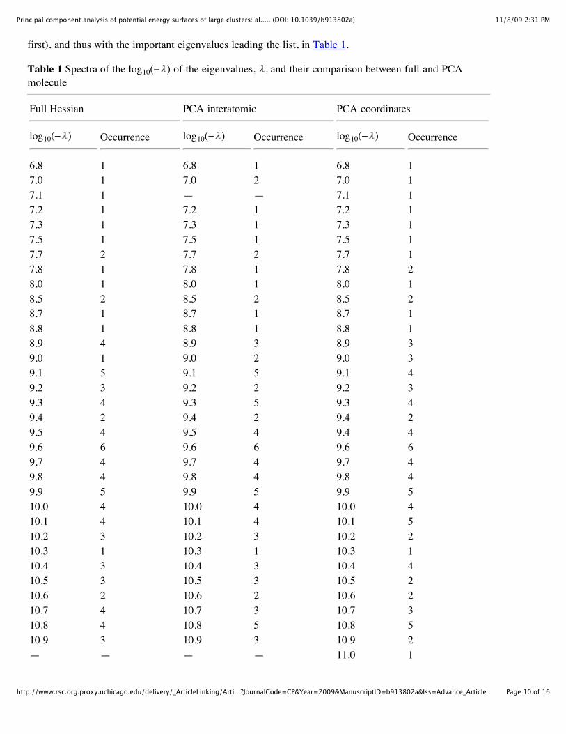
first), and thus with the important eigenvalues leading the list, in Table 1.

Table 1 Spectra of the log10(− ) of the eigenvalues, , and their comparison between full and PCAmolecule

Full Hessian PCA interatomic PCA coordinates

log10(− ) Occurrence log10(− ) Occurrence log10(− ) Occurrence

6.8 1 6.8 1 6.8 17.0 1 7.0 2 7.0 17.1 1 — — 7.1 17.2 1 7.2 1 7.2 17.3 1 7.3 1 7.3 17.5 1 7.5 1 7.5 17.7 2 7.7 2 7.7 17.8 1 7.8 1 7.8 28.0 1 8.0 1 8.0 18.5 2 8.5 2 8.5 28.7 1 8.7 1 8.7 18.8 1 8.8 1 8.8 18.9 4 8.9 3 8.9 39.0 1 9.0 2 9.0 39.1 5 9.1 5 9.1 49.2 3 9.2 2 9.2 39.3 4 9.3 5 9.3 49.4 2 9.4 2 9.4 29.5 4 9.5 4 9.4 49.6 6 9.6 6 9.6 69.7 4 9.7 4 9.7 49.8 4 9.8 4 9.8 49.9 5 9.9 5 9.9 510.0 4 10.0 4 10.0 410.1 4 10.1 4 10.1 510.2 3 10.2 3 10.2 210.3 1 10.3 1 10.3 110.4 3 10.4 3 10.4 410.5 3 10.5 3 10.5 210.6 2 10.6 2 10.6 210.7 4 10.7 3 10.7 310.8 4 10.8 5 10.8 510.9 3 10.9 3 10.9 2— — — — 11.0 1

http://www.rsc.org.proxy.uchicago.edu/delivery/_ArticleLinking/ArticleLinking.cfm?JournalCode=CP&Year=2009&ManuscriptID=b913802a&Iss=Advance_Article#tab1



11.1 2 11.1 2 11.1 111.2 2 11.2 3 11.2 411.3 3 11.3 2 11.3 211.4 3 11.4 3 11.4 411.5 1 11.5 1 11.5 111.6 1 11.6 1 — —

As one can see, there is a very close numerical relationship between the spectra, with almost identicalresults that differ in eigenvalue numbers by at most 0.1 and in occurrence by at most 2, with the vastmajority not differing at all. Again, the relaxation curves are in an even better agreement with the fullHessian method, as seen below.

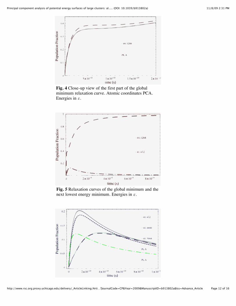
The master equation solutions given as relaxation curves, Pi(t), give a better picture of how well thePCA methods did. We set up the relaxation by picking out the top tier of highest energy levels in oursample PES for Ar13 which were well separated from the rest. We then divided the starting populationequally among them and let them relax. This seemed to be an initial condition that would be least likelyto introduce a bias in the relaxation process, and, at this stage, a detailed exploration of the effects of theinitial conditions seemed to be a second-level problem, something to address in later studies. In orderto understand the results better, it is important to note that the global minimum for Ar13 is not only in avery deep well and its energy is significantly lower than even the next closest minimum, but it is also byfar the most connected (almost three times more connected than the next closest one). Connectednessplays a very important role in the relaxation, as it dictates how much and how fast population is dumpedin and out of a minimum. So, for example, a higher energy minimum that is well connected will populatefast initially but will quickly lose that population and go to zero fast. Also, a low energy minimum that iswell connected, with most channels dumping into it from higher energy minima than depopulating it tolower energy minima, will build up population fast and then depopulate slower and have a higherpopulation left in it at infinite time. Obviously, since the global minimum is the most connected, it has amuch lower energy than anything else, and does not dump its population anywhere else, it will grow fastand approach a population fraction of 1 rapidly. Since the PCA methods gave results almost identical toeach other and to the full Hessian method, we only graph either the Pi(t) that play an important roleand/or the PCA methods for them that deviate from the full Hessian or each other. All PCA curves aresolid lines and all curves go to zero except for the global minimum.

The most important relaxation curve is that of the global minima, where all the population quicklyends up, for reasons stated above. Only the atomic coordinate method of PCA differed from the fullHessian for the global minimum. As can be seen in Fig. 4, the atomic coordinate method differs veryslightly from the full treatment. The low energy and connectivity of the global minima allow it todominate even the next closest minimum, which is both at a much higher energy and less than 1/3 theconnectivity, as shown in Fig. 5. The lowest tier of energy (excluding the global minimum), which arealso the most connected, are shown in Fig. 6. They populate well initially and go to zero much slowerthan the other minima, for reasons stated above. Again, only the atomic coordinate PCA differs from thefull Hessian method on two of the minima. The second tier of lowest energy levels are shown in Fig. 7.These have much lower maximum population levels than those in Fig. 6 and go to zero much faster. Forcomparison, we have the two minima that are the second most connected (i.e. lower than those in Fig. 6)shown in Fig. 8 and Fig. 10 of the ESI. The difference in the atomic coordinate PCA is shown in Fig. 8,while the highest energy tier that start with equal populations are shown in Fig. 9. We have included moregraphs in the ESI.














Fig. 4 Close-up view of the first part of the globalminimum relaxation curve. Atomic coordinates PCA.Energies in .

Fig. 5 Relaxation curves of the global minimum and thenext lowest energy minimum. Energies in .



Fig. 6 Relaxation curves of the lowest energy levels(also the most connected), excluding the globalminimum. Atomic coordinates PCA. Energies in .

Fig. 7 Relaxation curves of the energy levels just abovethe lowest ones. Energies in .

Fig. 8 Relaxation curves of second most connectedminima (second to the lowest energy tier). Atomiccoordinates PCA. Energies in .



Fig. 9 Relaxation curves of the top energy tier, whichwere all equally populated at t = 0. Energies in .

From the relaxation curves, we see that the two PCA methods give almost exact curves to the fullHessian methods and to each other. The only difference of the PCA methods are shown above, which arefew in number and differ only slightly. The only real difference between the two PCA methods is fact that

the coordinate method is much faster (requiring 3N × 3N covariance matrices versus matrices), while the interatomic has a slight advantage in accuracy. The enormous speed advantage of theatomic coordinate method, especially for medium sized and above systems, means that it is the preferredmethod. The accurate eigenvalues and master equation solutions mean that PCAs give the same set ofimportant dynamics as the case where we did not use them. However, their usefulness is currently limitedsince their speed advantage comes into play for systems much larger than those currently being studiedcomputationally, as discussed in the conclusion.

4 Conclusion

Both PCA and PCO offer a way to reduce the dimensionality of a data set. PCO was successfully used toprovide a 3D graph of the PES of Ar20. The graph showed that the PES of Ar20 is made up of two mainfunnels. PCA was used to reduce the dimensionality of the vibrational partition function, for purposes ofcomputing rate coefficients for the master equation. The rate constants were then used to get theeigenvalues of the master equation. The eigenvalue spectrum and master equation solutions obtained byusing PCA were almost identical to using the full Hessian. These proved that PCA is a valid way toreduce the dimensionality of the Hessian and obtain effective partition functions for use in the transitionmatrix of the master equation. The striking similarity of the eigenvalues from PCA and the full set ofcoordinates gave clear evidence that passage between a minimum and a specific saddle above thatminimum can be expressed very effectively in terms of a single variable—but a different variable forevery minimum–saddle pair. Although PCO and PCA were both successful for their intended purposes,PCA is nonetheless not recommended for use in calculating rate constants for many situations, asexplained below.

First, in constructing a PES for a cluster, all the Hessian eigenvalues, at least at the stationary points,are typically calculated as part of the search methods. For example, the database provided by Mark Milleret al.10 included the products of all the eigenvalues of the individual minima and saddles, this beingsuitable for calculating the vibrational partition functions. Therefore, the only potential use for anymethod that calculates Hessian eigenvalues from the PES database (including PCA) is a case in whichone does not have the eigenvalues used in constructing the PES, which is rare (if not an impossibility).

Second, calculations using the full Hessian methods require that we only diagonalize the Hessian oncefor each stationary point. However, the PCA method means we have to compare each saddle–minimum




pair to find the most significant changes and calculate the Hessian for the minimum and the saddle in thatpair based on the result of the comparison. Therefore, while for a minimum–saddle–minimum, the fullHessian method diagonalizes three 3N × 3N matrices, the atomic coordinates PCA method first needs todiagonalize two 3N × 3N covariance matrices and then diagonalize four reduced Hessian matrices ofabout the size of N × N.

Even with the computational cost advantages when one uses the Lanczos method to cut down on thecomputation of obtaining the three largest eigensystems of the two 3N × 3N covariance matrices anddiagonalizing the smaller N × N Hessians, the sheer number of extra calculations involved for the PCAmeans it will only see advantages for very large PES databases. At those large PES database sizes, theLanczos method becomes many orders of magnitude cheaper than full diagonalization and the smallersize of the PCA reduced Hessians outpace the fact that more of them need to be calculated. The point atwhich those two computational savings of the PCA overtake the full Hessian method is very dependent onthe algorithm and computational platform. Processor speed and architecture, RAM availability, operatingsystem, and parallel computing make the most significant impact on the turn-over point. Therefore, ourresults must be taken as very rough guides and the only way to get a more accurate estimate of what theturning point would be for a computing system is to run speed tests on that system.

In calculating the crossover point for the PCA methods, we biased the calculation toward the PCAmethod by using very conservative estimates and equations for things such as the number of saddles inthe database versus the number of minima and the advantage of using Lanczos method. Based on thetimings obtained on the computational resources available to us, our estimates give us a rough point of aPES the size of that of the full PES of Ar200 to Ar250. Note that the important factors are the size of thePES database, the relative ratio of the number of saddles to the number of minima, and the size of theHessian matrices, so if one uses a sampled PES, it needs to be at least the size of the full PES of theabove argon systems with the number of saddles not significantly larger than those in the argon systems.Since we estimate the Ar200 to have at least 7×1047 minima and 4×1050 saddles connecting those minima,and the largest current databases are not even in the millions, the PCA method will not be of any use fora very long time.

References

1 R. S. Berry and R. Breitengraser-Kunz, Phys. Rev. Lett., 1995, 74, 3951 [Links].2 R. E. Kunz and R. S. Berry, J. Chem. Phys., 1995, 103, 1904 [Links].3 K. D. Ball, R. S. Berry, R. E. Kunz, F. Y. Li, A. Proykova and D. J. Wales, Science, 1996, 271, 963

[Links].4 D. Wales, Energy Landscapes, Cambridge University Press, Cambridge, 2003.5 C. J. Tsai and K. D. Jordan, J. Phys. Chem., 1993, 97, 11227 [Links].6 J. Lu, C. Zhang and R. S. Berry, Phys. Chem. Chem. Phys., 2005, 7, 3443 [Links].7 K. D. Ball and R. S. Berry, J. Chem. Phys., 1999, 111, 2060 [Links].8 D. J. Wales, Mol. Phys., 2002, 100, 3285 [Links].9 D. J. Wales, J. P. K. Doye, M. A. Miller, P. N. Mortenson and T. R. Walsh, Adv. Chem. Phys., 2000,

115, 1.10 J. P. K. Doye, M. A. Miller and D. J. Wales, J. Chem. Phys., 1999, 111, 8417 [Links].11 J. C. Gower, Biometrika, 1966, 53, 325.12 I. T. Jolliffe, Principal Component Analysis, Springer, Berlin, 2002.13 N. G. van Kampen, Stochastic Processes in Physics and Chemistry, Elsevier, Amsterdam, 1981.14 K. D. Ball and R. S. Berry, J. Chem. Phys., 1998, 109, 8557 [Links].15 M. A. Miller, J. P. K. Doye and D. J. Wales, Phys. Rev. E: Stat. Phys., Plasmas, Fluids, Relat.

Interdiscip. Top., 1999, 60, 3701 [Links].

http://www.rsc.org.proxy.uchicago.edu/delivery/_ArticleLinking/citationresolver.cfm?artID=1228540




http://xlink.rsc.org.proxy.uchicago.edu/?doi=b508556j








16 Y. Levy, J. Jortner and R. S. Berry, Phys. Chem. Chem. Phys., 2002, 4, 5052 [Links].17 O. M. Becker and M. Karplus, J. Chem. Phys., 1997, 106, 1495 [Links].18 D. C. Rapaport, The Art of Molecular Dynamics Simulation, Cambridge University Press, 2004.19 P. B. Balbuena and J. M. Seminario, Molecular Dynamics (Theoretical and Computational

Chemistry), Elsevier Science, Amsterdam, 1999.20 Andrew Leach, Molecular Modeling: Principles and Applications, Prentice Hall, Englewood Cliffs,

New Jersey, 2nd edn, 2001.21 P. J. Robinson and K. A. Holbrook, Unimolecular Reactions, Wiley-Intersceince, London, 1972.22 R. G. Gilbert and S. C. Smith, Theory of Unimolecular and Recombination Reactions, Blackwell

Scientific, Oxford, 1990.23 Keith D. Ball and R. Stephen Berry, J. Chem. Phys., 1998, 109, 8541 [Links].24 F. Murtagh and A. Heck, Multivariate Data Analysis, Kluwer Academic, Dordrecht, 1987.25 Lindsay I. Smith, A Tutorial on Principal Components Analysis, URL

http://csnet.otago.ac.nz/cosc453/student_tutorials/principal_components.pdf, 2002.26 J. Edward Jackson, A User s Guide to Principal Components, John Wiley & Sons Inc., New Jersey,

2003.27 Louis Komzsik, The Lanczos Method: Evolution and Application, Society for Industrial & Applied

Mathematics, New York, 2003.28 J. P. K. Doye and D. J. Wales, J. Chem. Phys., 1995, 102, 9659 [Links].29 Alston S. Householder, Unitary Triangularization of a Nonsymmetric Matrix, J. Assoc. Comput.

Mach., 1958, 5(4), 339–342 [Links].30 Roger A. Horn and Charles R. Johnson, Matrix Analysis, Cambridge University Press, Cambridge,

1985.

Footnotes

Electronic supplementary information (ESI) available: Relaxation curves of second most connected minima; relaxation curvesof some middle energy tier minima which have better maximum population achieved than the rest of the middle tier; relaxationcurves of some middle energy tier minima which have better maximum population achieved than the rest of the middle tier;relaxation curves of some middle energy tier minima; some of the relaxation curves of the energy tier below the highest energytier. See DOI: 10.1039/b913802a

QR decomposition is the transformation of a matrix A into the product of an upper triangular matrix Q and an orthogonal matrixR.

This journal is © the Owner Societies 2009

http://xlink.rsc.org.proxy.uchicago.edu/?doi=b203534k





http://xlink.rsc.org.proxy.uchicago.edu/?DOI=b913802a

0.5 Supplementary

The the difference in the interatomic distance PCA is shown in Figure 10. Forthe middle energy tier, we list the ones that have the best maximum populationfor the tier in Figure 11/Figure 12 and we list some sample other middle tierminima in Figure 13/Figure 14. The difference in the atomic coordinate PCAare shown in Figure 11 and Figure 13, while the interatomic distance PCA areshown in Figure 12 and Figure 14. Finally, the highest energy tier that start withequal population are shown in Figure 9 and the energy tier just below them areshown in Figure 15. Note that the top high energy tier minima all relax exactlythe same, probably since they have very similar energies and connectivities.

27

Supplementary Material (ESI) for PCCPThis journal is © the Owner Societies 2009

0 1´10-10 2´10-10 3´10-10 4´10-10

time HsL

0

0.01

0.02

0.03

0.04

0.05

0.06

Po

pu

lati

on

Fra

cti

on

PCA

-40.6155

-40.6702

Figure 10: Relaxation curves of second most connected minima (second to thelowest energy tier). Interatomic PCA. Energies in ε.

28


0 2´10-11 4´10-11 6´10-11 8´10-11

time HsL

0

0.001

0.002

0.003

0.004

0.005

0.006

0.007

Po

pu

lati

on

Fra

cti

on

PCA

PCA

-39.4695

-39.5893

Figure 11: Relaxation curves of some middle energy tier minima which havebetter maximum population achieved than the rest of the middle tier. AtomicCoordinates PCA. Energies in ε.

29


0 2´10-11 4´10-11 6´10-11 8´10-11

time HsL

0

0.001

0.002

0.003

0.004

0.005

0.006

0.007

Po

pu

lati

on

Fra

cti

on

PCA

PCA

-39.4695

-39.5893

Figure 12: Relaxation curves of some middle energy tier minima which have bet-ter maximum population achieved than the rest of the middle tier. InteratomicPCA. Energies in ε.

30


0 5´10-10 1´10-9 1.5´10-9 2´10-

time HsL

0

0.0001

0.0002

0.0003

0.0004

0.0005

Po

pu

lati

on

Fra

cti

on

PCA

PCA

-39.2572

-39.4691

-39.5296

-40.1281

Figure 13: Relaxation curves of some middle energy tier minima. Atomic Co-ordinates PCA. Energies in ε.

31


0 5´10-10 1´10-9 1.5´10-9 2´10-9

time HsL

0

0.0001

0.0002

0.0003

0.0004

0.0005

Po

pu

lati

on

Fra

cti

on

PCA

PCA

-39.2572

-39.4691

-39.5296

-40.1281

Figure 14: Relaxation curves of some middle energy tier minima. InteratomicPCA. Energies in ε.

32


0 1´10-11 2´10-11 3´10-11 4´10-11 5´10-11 6´10-11

time HsL

0

0.005

0.01

0.015

0.02

Po

pu

lati

on

Fra

cti

on

-36.2863

-36.3161

-36.3267

Figure 15: Some of the relaxation curves of the energy tier below the highestenergy tier. Energies in ε.

33


principal component analysis of potential energy surfaces of large

Documents