the principal component analysis

The Principal Component Analysis

Philippe B. Laval

KSU

Fall 2015

Philippe B. Laval (KSU) PCA Fall 2015 1 / 25

Introduction

Every 80 minutes, the two Landsat satellites go around the world,recording images of our planet along a 185 Kim wide path. Every 16days, each satellite covers the entire surface of the planet. Every 8days, every single location on the planet can be monitored.These images can be used by urban planners to study the rate anddirection of population growth. They can be used to analyze soilmoisture, vegetation growth, lakes and rivers. Governments can usethem to detect and assess damages from natural disasters...Sensors on board the satellites acquire seven simultaneous images ofevery region by recording energy from separate wavelength bands.Each image is digitized and stored as a matrix., each numberindicating the signal intensity of the corresponding pixel. Each of theseven image is one channel of a multichannel or multispectral image.The seven images of one fixed region typically contains redundantinformation. Yet, certain features will only appear in one or twoimages because their color or temperature was only captured by twoof the seven sensors.


Introduction

Principal Component Analysis (PCA) is an effective way tosuppress redundant information and provide in only one or twocomposite images most of the information from the initial data.Roughly speaking, the goal is to find a special linear combination ofthe images that combines each pixel of the seven images into onesingle new pixel.

PCA can be applied to any data that consists of lists ofmeasurements made on a collections of objects or individuals.

For example, consider a chemical process that produces a plasticmaterial. To monitor the process, 300 samples of the materialproduced are taken and each sample is subject to a battery of eighttests. The lab report for each sample is a vector in R8 (8 tests).Since there are 300 samples, the set of these vectors is a 8× 300matrix. Such a matrix is called the matrix of observations. Looselyspeaking, we say that the process control data is eighth-dimensional.


Introduction

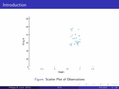
ExampleSuppose we have N college students for which we record their weights andheights. This is an example of a two-dimensional data. Let Xj be the

observation vector in R2 for the j th student that is Xj =

[wjhj

]where wj

is the weight and hj is the height of the jth student. Then, the matrix of

observations has the form[w1 w2 · · · wNh1 h2 · · · hN

]= [X1 X2 · · · XN ]. Here

is a possible matrix of observations (randomly generated with height inmeters and weight in kilograms) for N = 25 visualized on a scatter graphshown on the next slide.


Introduction

Figure: Scatter Plot of Observations


Mean and Covariance

Definition (Sample Mean)

Let [X1 X2 · · · XN ] be a p × N matrix of observations (meaning that foreach object, we have p observations, the Xi are p × 1 vectors). Thesample mean M of the observation vectors X1,X2, ...,XN is given by

M =1N

N∑i=1

Xi

The reader will note that M is also a p × 1 vector.

Geometrically, the sample mean is the point at the "center" of the scatterplot.For i = 1, 2, ...,N, we define X̂i = Xi −M and B =

[X̂1 X̂2 · · · X̂N

]. The

columns of B have a zero sample mean.


Mean and Covariance

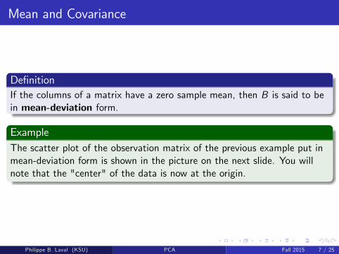
DefinitionIf the columns of a matrix have a zero sample mean, then B is said to bein mean-deviation form.

ExampleThe scatter plot of the observation matrix of the previous example put inmean-deviation form is shown in the picture on the next slide. You willnote that the "center" of the data is now at the origin.


Mean and Covariance

Figure: Observation Data in Mean-Deviation form


Mean and Covariance

DefinitionThe sample covariant matrix or the covariant matrix is the p × pmatrix defined by

S =1

N − 1BBT

Since any matrix of the form BBT is symmetric and positive semidefinite,so is S . Recall that a matrix A is positive definite (positive semidefinite) iffor every nonzero vector x, xTAx > 0 (xTAx ≥ 0).


Mean and Covariance

ExampleSuppose that measurements are made on 4 individuals and the observationvectors are

X1 =

121

, X2 =

4213

, X3 =

781

, X4 =

845

Compute the sample mean and the covariant matrix.


Mean and Covariance

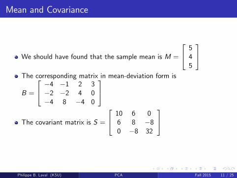
We should have found that the sample mean is M =

545

The corresponding matrix in mean-deviation form is

B =

−4 −1 2 3−2 −2 4 0−4 8 −4 0

The covariant matrix is S =

10 6 06 8 −80 −8 32


Mean and Covariance

We now discuss the meaning of the entries in S , the covariant matrix. Wecontinue using the notation developed in this section.

Let S = [sij ] and let X represent a vector that varies over the set ofobservation vectors X1,X2, ...,XN . Let’s denote the coordinates of Xby x1, x2, ..., xp . Recall, p is the number of observations. Then, x1 forexample, is a scalar that varies over the 1st coordinates ofX1,X2, ...,XN . Similarly, x2 is a scalar that varies over the 2ndcoordinates of X1,X2, ...,XN and so on.


Mean and Covariance

Definition (variance)For i = 1, 2, ..., p, the diagonal entry sii is called the variance of xi

The variance of xj measures the spread of the values of xj . In theexample above, from our computations, the variance of x1 is 10, thevariance of x2 is 8 and the variance of x3 is 32. What is importanthere is the relative size of these numbers. The fact that 32 > 10indicates that the set of third entries contains a wider spread than theset of first entries.

Definition (total variance)The total variance of the data is the sum of the diagonal entries in S .For a square matrix S (recall S is p × p), the sum of the diagonal entriesis called the trace of S and is denoted tr (S). Thus

total variance = tr (S)


Mean and Covariance

Definition (covariance)The entry sij for i 6= i , in S is called the covariance of xi and xj .

In the example above, looking at S , we see that the covariancebetween entries 1 and 3 is 0. This means that x1 and x3 areuncorrelated.


PCA Using Eigenvalues

As above, let us assume that our orinal variables are represented by thep × 1 vector X and we perform N measurements we denote X1,X2, ...,XN .For simplicity, we will assume that the p × N matrix of observations[X1 X2 · · · XN ] is already in mean-deviation form. If this were not thecase, the first step would be to put it in that form.The goal of PCA is to find an orthogonal p × p matrix, P = [u1 u2 ... up ]that determines a change of variables X = PY that is

x1x2...xp

= [u1 u2 ... up ]

y1y2...yp

with the property that the new variables y1, y2, ..., yp are uncorrelated andare arranged in order of decreasing variance.



The orthogonal change of variable X = PY means that eachobservation vector Xi is transformed into a new vector we call Yi suchthat Xi = PYi . Therefore, Yi = P−1Xi = PTXi since P is supposedto be orthogonal. This is true for i = 1, 2, ...,N.

It is not hard to see (see homework) that for each orthogonal matrixP, the covariant matrix for Y1,Y2, ...,YN is PT SP. So, the desiredorthogonal matrix P is the one that makes PT SP diagonal.

Let D be a diagonal matrix with the eigenvalues λ1, λ2, ..., λp of S onthe diagonal arranged so that λ1 ≥ λ2 ≥ ... ≥ λp ≥ 0 and let P be anorthogonal matrix whose columns are the unit eigenvectorsu1,u2, ...,up corresponding to the eigenvalues λ1 ≥ λ2 ≥ ... ≥ λp .Then, S = PDPT and D = PT SP.



DefinitionThe unit eigenvectors u1,u2, ...,up of the covariant matrix S are called theprincipal components of the data in the matrix of observations. Thefirst principal component is the eigenvector corresponding to the largesteigenvalue of S . The second principal component is the eigenvectorcorresponding to the second largest eigenvalue of S and so on.

The first principal component u1 determines the new variable y1 inthe following way. Let c1, c2, ..., cp be the entries in u1. Since uT1 isthe first row of PT , the equation Y = PTX shows that

y1 = uT1 X =

p∑i=1

cixi

Thus y1 is a linear combination of the original variable using theentries in u1 as weights. In a similar way, u2 determines the entries iny2, and so on.


PCA Using Eigenvalues: Summary

Given a matrix of observation B = [X1 X2 · · · XN ] which is assumed to bein mean-deviation form, to perform a principal component analysis, we dothe following:

1 Find the covariant matrix S =1

N − 1BBT

2 Diagonalize S using eigenvalues. We let λ1, λ2, ..., λp be theeigenvalues of S arranged so that λ1 ≥ λ2 ≥ ... ≥ λp ≥ 0 and let Pbe an orthogonal matrix whose columns are the unit eigenvectorsu1,u2, ...,up corresponding to the eigenvalues λ1 ≥ λ2 ≥ ... ≥ λp .

3 The unit eigenvectors u1,u2, ...,up of the covariant matrix S arecalled the principal components of the data in the matrix ofobservations.

4 The new uncorrelated variables are defined by Y = PTX where Y ,likeX is p × 1. The covariance of Y is PT SP.

5 The components y1, y2, ..., yp of y can be expressed in terms of thecomponents x1, x2, ..., xp of X by y1 = uTi X .



ExampleSuppose the covariant matrix of some data is

S =

2382.78 2611.84 2136.202611.84 3106.47 2553.902136.20 2553.90 2650.71

. Find the principal components ofthe data, list the new variable determined by the first principal componentand give the diagonal form of S .


Dimension Reduction

PCA is valuable when most of the variation in the data is due tovariations in only a few of the new variables y1, y2, ..., yp .

It can be shown that an orthogonal change of variables X = PY doesnot change the total variance of the data. This means that ifS = PDPT then{

total varianceof x1, x2, ..., xp

}=

{total varianceof y1, y2, ..., yp

}= tr (D)

= λ1 + λ2 + ...+ λp

The variance of yi is λi , and the quotientλi

tr (S)measures the

fraction of the total variance captured by yi .


Dimension Reduction

ExampleIn the example above, compute the various percentages of variancecaptured by each variable.

ExampleConsider the following data:

Boy #1 #2 #3 #4 #5

Weight (lb) 120 125 125 135 145Height (in) 61 60 64 68 72

1 Find the covariant matrix for the data.2 Make a principal component analysis of the data to find a single sizeindex that explains most of the variation in the data.


PCA Using SVD

The goal is the same as above, what changes is how we achieve it. Asabove, we will assume that the p × N matrix of observations[X1 X2 · · · XN ] is already in mean-deviation form. If this were not thecase, the first step would be to put it in that form. Assume the SVD ofthe matrix of observations [X1 X2 · · · XN ] is UΣV T . Here, U is p × p, Σis p × N and V T is N × N hence V is N × N. We define the new variableY by X = UY or Y = UTX . It can be shown that the variance of Y is1

N − 1Σ2 which is already in diagonal form; this is what we wanted. In

this case, the principal components will be the columns of U. If we letU = [u1 u2 ... up ] then the equation Y = PTX shows that

y1 = uT1 X =

p∑i=1

cixiwhere c1, c2, ..., cp are the entries in u1. Thus y1 is a

linear combination of the original variable using the entries in u1 asweights. In a similar way, u2 determines the entries in y2, and so on.


PCA Using SVD: Summary

Given a matrix of observation B = [X1 X2 · · · XN ] which is assumed to bein mean-deviation form, to perform a principal component analysis, we dothe following:

1 Find a SVD for B, say B = UΣV T .2 If we let U = [u1 u2 ... up ] then we define Y = UTX . The

covariance of Y is1

N − 1Σ2. Y is the new uncorrelated variable.

3 We let λ1, λ2, ..., λp be the diagonal elements of1

N − 1Σ2

(automatically arranged so that λ1 ≥ λ2 ≥ ... ≥ λp ≥ 0). Then λi isthe varaince of yi which is also the variance of xi .

4 The unit vectors u1,u2, ...,up are called the principal componentsof the data in the matrix of observations.

We can get all the components we were able to get with the eigenvaluediagonalization. We simply got them differently. MATLAB uses thistechnique as it is a little bit more robust than the eigenvalue method.


PCA and MATLAB

Newer versions of MATLAB have a function to perform this, it is calledpca. You can get help for it in MATLAB. Two important things toremember about MATLAB’s pca:

1 It uses the SVD approach to find the principal components andrelated information.

2 It works differently than what is explained in these notes in thefollowing sense. MATLAB’s matrix of observation is the transpose ofthe matrix of observations used in these notes. In other words, thecolumns of our matrix of observations contain the various variablesused for our data. For MATLAB, these variables are stored as therows of the matrix of observations.

Suppose that A is our matrix of observations. To use MATLAB’s PCA,use pca(A’), where A′ is the transpose of A.


Exercises

See the problems at the end of the notes on Principal Component Analysis.


http://math.kennesaw.edu/~plaval/math4490/fall2015/SVD_PCA.pdf

the principal component analysis

Documents