classical and robust symbolic principal component analysis ... · classical and robust symbolic...
TRANSCRIPT

Classical and Robust Symbolic Principal
Component Analysis for Interval Data
Margarida Azeitona Sequeira Vilela
Thesis to obtain the Master of Science Degree in
Mathematics and Applications
Supervisor: Doctor Maria do Rosario de Oliveira Silva
Examination Committee
Chairperson: Doctor Antonio Manuel Pacheco PiresSupervisor: Doctor Maria do Rosario de Oliveira Silva
Members of the Committee: Doctor Maria Paula de Pinho de Brito Duarte Silva
December 2015


Resumo
A analise em componentes principais e um dos metodos estatısticos mais populares para analisar
dados reais. Por este motivo, tem havido varias propostas para estender esta metodologia para o
enquadramento da analise de dados simbolicos, nomeadamente para dados intervalares.
Nesta tese, deduzimos as formulacoes populacionais para quatro destes algoritmos: Metodo dos
Centros, Metodo dos Vertices, Complete Information Principal Component Analysis and Symbolic
Covariance Principal Component Analysis. Com base nessas formulacoes teoricas, propomos uma
metodologia geral que fornece simplificacoes, conhecimento adicional e unificacao dos metodos discu-
tidos. Adicionalmente, e derivada uma formula explıcita e simples para a definicao dos scores das
componentes principais simbolicas, equivalente a representacao por Maximum Covering Area Rectan-
gles.
Alem disso, a existencia de observacoes atıpicas poderia distorcer as componentes principais
simbolicas amostrais e os respetivos scores. Para ultrapassar este problema, propomos duas famılias
de metodos robustos para analise em componentes principais simbolicas: um baseado em matrizes
de covariancia robustas e outro baseado em Projection Pursuit. E efetuado um estudo de simulacao
para avaliar o desempenho desses procedimentos, que nos permite concluir que estes podem acomodar
pequenos desvios do modelo central especificado.
Finalmente, para que todas estas novas metodologias propostas sejam facilmente utilizadas na
analise de dados reais, desenvolvemos uma aplicacao web, utilizando a plataforma Shiny do R. Na
nossa aplicacao, de forma interativa, e possıvel analisar, visualizar e comparar os resultados das com-
ponentes principais classicos e robustas, para dados convencionais e dados intervalares. Ilustramos
algumas das suas potencialidades com um conjunto de dados das telecomunicacoes.
Palavras-chave: Analise de dados simbolicos, variaveis intervalares, analise em componentes
principais, estatıstica robusta.
i


Abstract
Principal component analysis is one of the most popular statistical methods to analyse real data.
Therefore, there have been several proposals to extend this methodology to the symbolic data analysis
framework, in particular to interval-valued data.
In this thesis, we deduce the population formulations of four of these algorithms: Centers Method,
Vertices Method, Complete Information Principal Component Analysis, and Symbolic Covariance
Principal Component Analysis. Based on these theoretical formulations, we propose a general method-
ology that provides simplifications, additional insight and unification of the discussed methods. Addi-
tionally, we derive an explicit and straightforward formula to define the symbolic principal component
scores, equivalent to the representation by Maximum Covering Area Rectangle.
Furthermore, the existence of atypical observations could distort the sample symbolic principal
components and correspondent scores. To overcome this problem, we propose two families of robust
methods for symbolic Principal Component Analysis: one based on robust covariance matrices and
another based on Projection Pursuit. A simulation study is conducted to access the performance
of these procedures, allowing us to conclude that they can accommodate small deviances from the
specified central model.
Finally, to make all the new proposed methodologies easily used in the analysis of real data, we
also developed a web application, using the Shiny web application framework forR. In our application
it is possible to interactively analyse, visualize, and compare results of classical and robust principal
components, in the conventional and interval-valued frameworks. We illustrate some of its potential-
ities with a Telecommunications dataset.
Keywords: Symbolic data analysis, interval-valued variables, principal component analysis,
robust statistics.
iii


Acknowledgments
First and foremost, I would like to thank my supervisor, Professor Rosario Oliveira for her support,
time, guidance and constructive criticism during all this work. It was a pleasure working with her and
a very enriching experience.
I would also like to thank Professor Antonio Pacheco for some interesting input into this work and
for the financial support provided by CEMAT, namely for attending some conferences.
Finally, special thanks to my close family and friends for all their support and care.
v


Contents
Resumo i
Abstract iii
Acknowledgments v
List of Figures ix
List of Tables xi
Acronyms xiii
1 Introduction 1
1.1 Motivation . . . . . . . . . . . . . . . . . . . . . . . . . . . . . . . . . . . . . . . . . . 1
1.2 Claim of contributions . . . . . . . . . . . . . . . . . . . . . . . . . . . . . . . . . . . . 2
1.3 Overview of the thesis . . . . . . . . . . . . . . . . . . . . . . . . . . . . . . . . . . . . 3
2 Symbolic Data Analysis 5
2.1 Types of data . . . . . . . . . . . . . . . . . . . . . . . . . . . . . . . . . . . . . . . . . 5
2.2 From classical to symbolic data . . . . . . . . . . . . . . . . . . . . . . . . . . . . . . . 7
2.3 Parametric models for interval data . . . . . . . . . . . . . . . . . . . . . . . . . . . . . 9
2.4 Descriptive Statistics . . . . . . . . . . . . . . . . . . . . . . . . . . . . . . . . . . . . . 11
3 Symbolic Principal Component Analysis 16
3.1 Introduction . . . . . . . . . . . . . . . . . . . . . . . . . . . . . . . . . . . . . . . . . . 16
3.2 SPCA Methods . . . . . . . . . . . . . . . . . . . . . . . . . . . . . . . . . . . . . . . . 18
3.2.1 CPCA . . . . . . . . . . . . . . . . . . . . . . . . . . . . . . . . . . . . . . . . . 19
3.2.2 VPCA . . . . . . . . . . . . . . . . . . . . . . . . . . . . . . . . . . . . . . . . . 20
3.2.3 SO-PCA: mixed Strategy . . . . . . . . . . . . . . . . . . . . . . . . . . . . . . 24
3.2.4 Midpoints and radii PCA . . . . . . . . . . . . . . . . . . . . . . . . . . . . . . 24
3.2.5 Interval PCA . . . . . . . . . . . . . . . . . . . . . . . . . . . . . . . . . . . . . 25
3.2.6 Complete Information PCA . . . . . . . . . . . . . . . . . . . . . . . . . . . . . 26
3.2.7 Symbolic Covariance PCA . . . . . . . . . . . . . . . . . . . . . . . . . . . . . . 28
vii
3.3 General form of the covariance matrix . . . . . . . . . . . . . . . . . . . . . . . . . . . 29
3.4 Representation of Symbolic Scores . . . . . . . . . . . . . . . . . . . . . . . . . . . . . 30
4 Robust Symbolic Principal Component Analysis 35
4.1 Sensitivity of SPC classical methods to atypical observations . . . . . . . . . . . . . . 36
4.2 Robust estimation methods . . . . . . . . . . . . . . . . . . . . . . . . . . . . . . . . . 38
4.2.1 Robust covariance matrix . . . . . . . . . . . . . . . . . . . . . . . . . . . . . . 38
4.2.2 Projection pursuit . . . . . . . . . . . . . . . . . . . . . . . . . . . . . . . . . . 41
4.3 Comparative study . . . . . . . . . . . . . . . . . . . . . . . . . . . . . . . . . . . . . . 43
5 Implementation 48
5.1 Conversion . . . . . . . . . . . . . . . . . . . . . . . . . . . . . . . . . . . . . . . . . . 49
5.2 Estimation methods and objects visualization . . . . . . . . . . . . . . . . . . . . . . . 51
5.3 A Shiny web application to analyse Telecommunications data . . . . . . . . . . . . . . 53
5.3.1 Conventional Analysis . . . . . . . . . . . . . . . . . . . . . . . . . . . . . . . . 56
5.3.2 Symbolic Analysis . . . . . . . . . . . . . . . . . . . . . . . . . . . . . . . . . . 58
6 Conclusions 62
6.1 General overview . . . . . . . . . . . . . . . . . . . . . . . . . . . . . . . . . . . . . . . 62
6.2 Future work . . . . . . . . . . . . . . . . . . . . . . . . . . . . . . . . . . . . . . . . . . 63
References 65
viii
List of Figures
2.1 Different formats of conventional data matrices. . . . . . . . . . . . . . . . . . . . . . . 5
2.2 Different hyper-rectangles (Adapted from [4]). . . . . . . . . . . . . . . . . . . . . . . 7
(a) p = 2. . . . . . . . . . . . . . . . . . . . . . . . . . . . . . . . . . . . . . . . . . . 7
(b) p = 3. . . . . . . . . . . . . . . . . . . . . . . . . . . . . . . . . . . . . . . . . . . 7
3.1 Algorithm of method CPCA. . . . . . . . . . . . . . . . . . . . . . . . . . . . . . . . . 19
(a) Input: Symbolic Objects. . . . . . . . . . . . . . . . . . . . . . . . . . . . . . . . 19
(b) Calculate the centers. . . . . . . . . . . . . . . . . . . . . . . . . . . . . . . . . . 19
(c) Use the centers as conventional data. . . . . . . . . . . . . . . . . . . . . . . . . . 19
(d) Obtain conventional PCs. . . . . . . . . . . . . . . . . . . . . . . . . . . . . . . . 19
(e) Project the centers on the new directions. . . . . . . . . . . . . . . . . . . . . . . 19
(f) Transform the scores into Symbolic Objects. . . . . . . . . . . . . . . . . . . . . 19
3.2 Algorithm of method VPCA. . . . . . . . . . . . . . . . . . . . . . . . . . . . . . . . . 20
(a) Input: Symbolic Objects. . . . . . . . . . . . . . . . . . . . . . . . . . . . . . . . 20
(b) Calculate the vertices. . . . . . . . . . . . . . . . . . . . . . . . . . . . . . . . . . 20
(c) Use the vertices as conventional data. . . . . . . . . . . . . . . . . . . . . . . . . 20
(d) Obtain conventional PCs. . . . . . . . . . . . . . . . . . . . . . . . . . . . . . . . 20
(e) Project the vertices on the new directions. . . . . . . . . . . . . . . . . . . . . . . 20
(f) Transform the scores into Symbolic Objects. . . . . . . . . . . . . . . . . . . . . 20
3.3 Representation of a symbolic object with p = 2 symbolic variables. . . . . . . . . . . . 21
3.4 Different representations of SPC scores (Source: [38]). . . . . . . . . . . . . . . . . . . 34
4.1 Density plots of the first eigenvalue for data with different levels of contamination. . . 37
(a) Data without contamination. . . . . . . . . . . . . . . . . . . . . . . . . . . . . . 37
(b) Data with 5% of contamination. . . . . . . . . . . . . . . . . . . . . . . . . . . . 37
(c) Data with 20% of contamination. . . . . . . . . . . . . . . . . . . . . . . . . . . . 37
4.2 Density plots of the first eigenvalue obtained for different contamination models. . . . 45
(a) Model: M0, ε = 0. . . . . . . . . . . . . . . . . . . . . . . . . . . . . . . . . . . . 45
(b) Model: MmC5, ε = 0.05. . . . . . . . . . . . . . . . . . . . . . . . . . . . . . . . 45
(c) Model: MmC5, ε = 0.2. . . . . . . . . . . . . . . . . . . . . . . . . . . . . . . . . 45
ix

4.3 MSE of the first eigenvalue obtained for the contamination model MmC3 and different
levels of contamination. . . . . . . . . . . . . . . . . . . . . . . . . . . . . . . . . . . . 46
4.4 ACV of the first eigenvector obtained for the contamination model MmC3 and different
levels of contamination. . . . . . . . . . . . . . . . . . . . . . . . . . . . . . . . . . . . 47
5.1 Available packages for SDA (blue) and conversion functions proposed (red). . . . . 52
5.2 Comparison between the two approaches - example. . . . . . . . . . . . . . . . . . . . 55
(a) Conventional data. . . . . . . . . . . . . . . . . . . . . . . . . . . . . . . . . . . . 55
(b) Interval-valued data. . . . . . . . . . . . . . . . . . . . . . . . . . . . . . . . . . . 55
5.3 Options available in the left panel - conventional approach. . . . . . . . . . . . . . . . 56
5.4 Example of a scatterplot - conventional approach. . . . . . . . . . . . . . . . . . . . . . 57
5.5 Options available in the left panel - symbolic approach. . . . . . . . . . . . . . . . . . 59
5.6 Example of a plot representing two symbolic variables - symbolic approach. . . . . . . 60
5.7 Scores Representation: PC1 vs. PC2 - Comparison between two SPCA methods. . . . 61
(a) CPCA. . . . . . . . . . . . . . . . . . . . . . . . . . . . . . . . . . . . . . . . . . 61
(b) VPCAgridQN. . . . . . . . . . . . . . . . . . . . . . . . . . . . . . . . . . . . . . 61
x
List of Tables
2.1 Symbolic data table with information of three universities (parte I). . . . . . . . . . . 6
2.2 Symbolic data table with information of three universities (parte II). . . . . . . . . . . 6
2.3 Conventional data matrix (Micro-data). . . . . . . . . . . . . . . . . . . . . . . . . . . 8
2.4 Interval data matrix (macro-data). . . . . . . . . . . . . . . . . . . . . . . . . . . . . . 9
2.5 Interval data matrix - centers and ranges parametrization. . . . . . . . . . . . . . . . . 10
2.6 Different configurations for Σ (Adapted from [9] and [25]). . . . . . . . . . . . . . . . . 11
2.7 Combinations of symbolic variances and covariances. . . . . . . . . . . . . . . . . . . . 15
3.1 Symbolic principal component estimation methods - Type of strategy. . . . . . . . . . 17
3.2 Coefficient Values for ΣM . . . . . . . . . . . . . . . . . . . . . . . . . . . . . . . . . . . 29
3.3 Symbolic principal component estimation methods - Type of representation. . . . . . . 30
5.1 Available packages for SDA. . . . . . . . . . . . . . . . . . . . . . . . . . . . . . . . 48
5.2 Symbolic Min-Max Data Frame. . . . . . . . . . . . . . . . . . . . . . . . . . . . . . . 49
5.3 Symbolic Data Table. . . . . . . . . . . . . . . . . . . . . . . . . . . . . . . . . . . . . 49
5.4 Symbolic Center-Range Data Frame. . . . . . . . . . . . . . . . . . . . . . . . . . . . . 50
5.5 Symbolic Center-Log(Range) Data Frame. . . . . . . . . . . . . . . . . . . . . . . . . . 50
5.6 Symbolic Array. . . . . . . . . . . . . . . . . . . . . . . . . . . . . . . . . . . . . . . . . 50
(a) First level - Matrix of minimums. . . . . . . . . . . . . . . . . . . . . . . . . . . . 50
(b) Second level - Matrix of maximums. . . . . . . . . . . . . . . . . . . . . . . . . . 50
5.7 Conversion functions proposed. . . . . . . . . . . . . . . . . . . . . . . . . . . . . . . . 51
5.8 Names of the functions implementing SPCA methods: classical and robust estimators. 51
xi


Acronyms
ACV Absolute Cosine Value.
CRAN Comprehensive R Archive Network.
IST Instituto Superior Tecnico.
MVE Minimum Volume Ellipsoid.
MCAR Maximum Covering Area Rectangle.
MCD Minimum Covariance Determinant.
MSE Mean Squared Error.
PC Principal Component.
PCA Principal Component Analysis.
PECS Parallel Edges Connected Shape.
PP Projection Pursuit.
RE Relative Error.
SDA Symbolic Data Analysis.
SPC Symbolic Principal Component.
SPCA Symbolic Principal Component Analysis.
TLE Trimmed Likelihood Estimator.
xiii

xiv

Chapter 1
Introduction
1.1 Motivation
In recent years we have witnessed a huge breakthrough of technology which enables the storage of a
massive amount of information. Additionally, the nature of the information collected is also changing.
In fact, besides the traditional format of recording single values for each observation, we have the
possibility to record lists, intervals, histograms or even distributions to characterize an observation.
However, conventional data analysis is not prepared for neither of these challenges, and does not have
the necessary or appropriate means to treat extremely large databases or data with a more complex
structure.
For example, if we collect data about elementary schools, one possible way to characterize each
school is by the number of students and the number of professors needed to teach these students, where
we assume that each professor is only responsible for teaching a class, which can include a variable
number of students. In a scenario like this we need to find a way to summarize this information
without omitting or losing relevant knowledge about the data. If we follow a conventional analysis we
would be tempted to describe each school by some summary statistic of the number of students by
teacher, but perhaps this would not be the most appropriate way to characterize this dataset.
Examples like this made it clear that it was necessary to come up with better alternatives and in
particular, develop a new framework to handle these new kinds of data. With this concern in mind,
Symbolic Data Analysis (SDA) was proposed by E. Diday in [17].
In this new framework, the data may have resulted from the aggregation of the individual ob-
servations (micro-data) by interest concepts or groups (macro-data) or are simply representations of
abstract categories. Moreover, many kinds of new variables were also introduced, for instance interval-
valued variables. In this new type of variable, instead of a single value for each observation we consider
an interval of real numbers.
In order to come up with new tools capable of analysing these new types of data, two European
research projects (SODAS 1 and ASSO 2) were developed with the collaboration of numerous teams,
from various countries. One of the major contributions resulting from these projects was the creation
1Symbolic Official Data Analysis System.2Analysis System of Symbolic Official data.
1

of SODAS, a software specially oriented for SDA.
Since then, the SDA community is growing, developing and adapting the concepts and the sta-
tistical methodologies applied in the conventional framework to the scope of SDA, so that this new
research area provides versatile tools to analyse real data.
Principal Component Analysis (PCA) is one of the most used statistical methods in the analysis
of real problems. Because of its popularity, in recent years there have been several proposes to extend
this methodology to the SDA framework, namely to interval-valued variables.
The methods CPCA (centers) and VPCA (vertices), pioneers in symbolic PCA [10], are the best
known examples of this family of methods. However, recently many other alternatives have emerged
in the literature (vide e.g. [38, 59]).
One common aspect to all these methods is the fact that they are all described by thorough
algorithms and their main purpose is to obtain sample symbolic principal components. Moreover,
there is no clear insight on the similarities and differences among the methods. So for a researcher
it is difficult to choose the most adequate method to solve a specific real problem. Usually, when
a simulation study is developed for comparison of Symbolic Principal Component Analysis (SPCA)
methods, the methods are compared with the “best” known method, due to the lack of theoretical
values to use as a benchmark. For all these reasons, we considered that it is essential to work on
the deduction of population formulations for the available symbolic principal component estimation
methods, in a attempt to get additional knowledge about the methods and the properties inherited
by the resulting principal components.
Another aspect that aroused our interest was the fact that, in the conventional framework, despite
all the advantages and potentialities of PCA, its results may be extremely sensitive to the presence of
outlying observations. And since the procedure of most of these symbolic Principal Component (PC)
estimation methods includes the estimation of the PCs in a conventional way, this may imply that
the symbolic methods are also affected by the presence of these atypical observations.
This last concern motivated us to assess the impact of outliers in the symbolic framework by
means of a simulation study, and if our suspicions prove to be true it is also necessary to invest in the
development of robust PC estimation methods for interval-valued data, based on procedures similar
to the ones used to attenuate this problem in the conventional framework.
1.2 Claim of contributions
In what follows, we can point out several contributions of our work.
• We formulate several definitions of sample symbolic variance and covariance for interval-valued
data, available in the literature, as a function of the centers and ranges. Using the weak law
of large numbers, we establish, for each definition, the population symbolic covariance matrix
as a function of the mean and covariances of the vectors of centers and ranges characterizing a
certain vector of random interval-valued variables.
2

• We obtain a population formulation for four Symbolic Principal Component (SPC) estimation
methods and propose a general and unifying methodology to compute them.
• We deduce a simple and straightforward formula to construct the SPC scores from the con-
ventional PC scores, equivalent to the representation by Maximum Covering Area Rectangles
(MCARs).
• We propose two approaches for robust SPC estimation methods:
(i) using projection pursuit methods;
(ii) based on a robust covariance matrix.
• We implement routines in the statistical software to compute the classical SPC estimation
methods and our robust proposals.
• We design routines to make conversions between the different representations of interval-valued
data used in several packages for SDA. With these it is easier to use functions from different
packages consecutively in the same analysis.
• We develop a web application using the Shiny web application framework for . This applica-
tion allows to interactively analyse, visualize, and compare results for descriptive statistics and
principal components in the conventional and symbolic frameworks. We illustrate its functioning
with a Telecommunications dataset.
1.3 Overview of the thesis
We conclude this introduction by presenting a summarized overview of this thesis. In Chapter 2
we introduce some basic concepts of SDA emphasising the main differences between conventional
and symbolic data. In particular, we focus on the study of descriptive statistics for interval-valued
variables. Special attention is given to the concepts of symbolic variance and covariance and theoretical
formulations of these estimators are derived. This chapter gives important tools to understand the
SPC estimation methods.
In Chapter 3 we revise the current SPC estimation methods and analyse four of them, clarifying
the underlying concepts and obtaining population formulations. A general and unifying formulation
of these methods is proposed. We conclude by discussing possible techniques used to define and
represent the SPC scores. The most popular of these methods, MCAR representation, is analysed,
and an explicit and population formulation is presented.
Chapter 4 starts with a review of some conventional robust PC methods and then, we propose
robust methods for interval-valued data based on these ideas and combined with the results of Chap-
ter 3. To conclude this chapter, a simulation study is conducted in order to evaluate the performance
of the classic and robust SPC estimators under study in the presence of small deviances from a central
model.
3

In Chapter 5 we present the functions for the statistical software [49] implemented during
this work. Particular attention is given to a web application (available at http://52.16.30.111/
shinyapp-marga/), develop by us using the Shiny web application framework for . Some potential-
ities of this application are illustrated with a Telecommunications dataset.
Finally, the general conclusions of this work as well as some directions to pursue in future research
are presented in Chapter 6.
4

Chapter 2
Symbolic Data Analysis
In this chapter we introduce some basic concepts of SDA, highlighting the differences between con-
ventional and symbolic data. We focus on the analysis of parametric models and descriptive statistics
that have been proposed for interval-valued variables.
2.1 Types of data
In the usual data analysis framework, called conventional in this thesis, each object is characterized
by one single value for each variable and data are organized in a (n × p) matrix (rows correspond
to objects, columns to variables). This data matrix may present one of the formats in Figure 2.1,
depending on the relation between the number of objects and the number of variables.
x11 · · · x1p...
. . ....
.... . .
......
. . ....
xn1 · · · xnp
n >> p
x11 · · · · · · · · · x1p... · · · · · · · · ·
...xn1 · · · · · · · · · xnp
p >> n
Figure 2.1: Different formats of conventional data matrices.
The variables are classified as qualitative, if the values are categories or quantitative if the values
are numbers. In the next example, we illustrate the use of different types of conventional variables.
Example 2.1.1. A student can be described by: (Adapted from [58])
• x1 - Average of his grades (continuous quantitative variable);
• x2 - Age (discrete quantitative variable);
• x3 - Gender (nominal categorical variable);
• x4 - Level of education (ordinal categorical variable).•
However, in some situations, this formulation does not adequately describe the phenomena since
it does not take into consideration possible intrinsic variability and uncertainty. To cope with this
situation, SDA proposed the introduction of new statistical units and variables that could take into
consideration potential variability inherent to the data.
5

Symbolic variables can be classified according to the following types, illustrated in Tables 2.1 and
2.2:
(a) Numerical multi-valued variable (e.g. Number of course changes);
(b) Categorical multi-valued variable (e.g. Sports teams);
(c) Interval variable (e.g. Age);
(d) Histogram variable (e.g. Number of years to graduate);
(e) Categorical modal variable (e.g. Gender)
It is worth mentioning that numerical single-valued variables and categorical single-valued variable
are conventional variables and particular cases of (a) and (b), respectively.
In this toy example, let us suppose that we have aggregated information such that the entities
under analysis are the universities and not the individual students of each university.
Table 2.1: Symbolic data table with information of three universities (parte I).
(a) (b) (c)i University Number of course changes Sports teams Age
1 A {0, 1} {None, Football, Basketball} [17,30]2 B {0, 1, 2} {None, Football, Swimming} [18,35]3 C {0} {None, Football, Basketball, Volleyball} [17,43]
Table 2.2: Symbolic data table with information of three universities (parte II).
(d) (e)i University Number of years to graduate Gender
1 A {[0, 4[, 0.25; [4, 6[, 0.65;≥ 6; 0.10} {F, 0.25; M, 0.75}2 B {[0, 4[, 0.35; [4, 6[, 0.45;≥ 6; 0.20} {F, 0.45; M, 0.55}3 C {[0, 4[, 0.15; [4, 6[, 0.80;≥ 6; 0.05} {F, 0.52; M, 0.48}
The definition of these new and more general types of variables was presented in Chapter 3 of [5].
In this work we only study interval-valued variables. Next, we present its definition using a notation
adapted from [5].
Definition 2.1. An interval-valued variable Xj is a mapping from a set E of statistical entities
(individuals or categories) into a set B of intervals of R:
Xj : E → B,
such thatXj(ei) = ξij ,∀ei ∈ E and ξi,j = [aij , bij ] ⊂ R, with aij ≤ bij .
Admitting that each entity in E can be characterized by p-interval-valued variables, X = (X1, . . . , Xp)t,
thus X(ei) = ξi, where ξi = (ξi1, . . . , ξip)t = ([ai1, bi1], . . . , [aip, bip])t.
Eventhough, in the literature, there are different notations to refer to the bounds of each interval.
In this thesis we will use aij for the lower bounds and bij for the upper bounds.
Let us consider a object, ei, characterized by p = 3 symbolic variables. That particular object
is described by ([ai1, bi1], [ai2, bi2], [ai3, bi3])t and can be graphically represented by a hyper-rectangle
with 2qi vertices, where qi is the number of non-trivial intervals, that is, the intervals for which
6

aij < bij . In that sense, a degenerate observation is defined as a symbolic object for which aij = bij ,
for at least one value of j (for at least one variable).
Possible hyper-rectangles for p = 3 are presented in Figure 2.2b and can be described, as follows:
• For H3 (parallelepiped) all the intervals are non-trivial (∀i ai 6= bi);
• For H2 (rectangle) one of the intervals is trivial (∃1i : ai = bi);
• For H1 (line segment) two of the intervals are trivial (∃1i : ai 6= bi);
• For H0 (point) all the intervals are trivial (∀i ai = bi). This is the special case of an observation
in R3.
All the above hyper-rectangles, except H3, are representations of degenerate observations. A
similar analysis can be conducted to p = 2 (see Figure 2.2a) and in this case, H2 corresponds to the
non-degenerate observation. As expected, in either case, H0 corresponds to a conventional observation.
(a) p = 2. (b) p = 3.
Figure 2.2: Different hyper-rectangles (Adapted from [4]).
2.2 From classical to symbolic data
Given the novelty of SDA is interesting to discuss, eventhough in a brief manner, the practical interest
of the symbolic approach.
When a researcher is faced with symbolic data, a simple strategy is to transform information
into a conventional format. For example, if we had three observations o1 = [26, 34], o2 = [28, 32]
and o3 = [2, 8], an appealing procedure is to consider the center of the intervals, obtaining c1 = 30,
c2 = 30, c3 = 5. But data transformed in this way do not distinguish objects 1 and 2, since they have
the same centers (c1 = c2), although o1 6= o2. If we only have observation o3 and we consider that the
micro-data follow a uniform distribution in [2, 8], then the variance associated with this observation
is 3. If we only consider the center of the interval in a classic perspective, then is like the micro-data
are equal to 5 with probability one, and its variance is 0. But o3 = [2, 8] tells that the micro-data
vary within [2, 8], thus admitting zero variability seems absurd in this case.
7

In general, SDA is preferably when we are interested in analysing data at a higher level (classes,
categories or concepts), rather than at individual level, but keeping the internal variability of the
individuals. Moreover, we may have native interval data when we are modelling daily stock prices
or temperatures, for instance. Another source of symbolic data is the aggregation of conventional
data, which allows considerable reduction in the size of data and thereby facilitates the analyse of
large databases. An additional benefit of aggregation is that, since we do not look at the individual
level, the confidentiality issues involved in analysing private data, for instance, official statistics, are
no longer a problem.
If the informations were gathered at the same time or the temporal instant is irrelevant the
aggregation of micro-data is called contemporary. If, on the contrary, the time was the aggregation
criterion we say that we are performing a temporal aggregation.
Furthermore, some authors argue that aggregation of conventional data is the most common source
of symbolic data. Thus, the process of analysing symbolic data, obtained from conventional data,
essentially consists in the following steps:
1. Consider a matrix of micro-data like the conventional data matrix in Table 2.3, where xik,j
represents the kth micro-observation associated with the individual i for the jth variable, with
i = 1 . . . , n, k = 1, . . . , ui, j = 1 . . . , p and ui is the number of micro-observations associated
with the ith individual.
Table 2.3: Conventional data matrix (Micro-data).
Variable 1 Variable 2 · · · Variable p
1
1 x11,1 x11,2 · · · x11,p2 x12,1 x12,2 · · · x12,p...
......
. . ....
u1 x1u1,1x1u1,2
· · · x1u1,p
2
1 x21,1 x21,2 · · · x21,p2 x22,1 x22,2 · · · x22,p...
......
. . ....
u2 x2u2,1x2u2,2
· · · x2u2,p
......
......
...
n
1 xn1,1 xn1,2 · · · xn1,p2 xn2,1 xn2,2 · · · xn2,p...
......
. . ....
un xnun,1 xnun,2 · · · xnun,p
2. Determine the concepts of interest in order to build the corresponding symbolic data table;
3. Aggregate the micro-data in accordance with the concepts defined, obtaining the macro-data.
Since we are only using interval-valued variables, the macro-data obtained have the format
specified in Table 2.4.
8

Table 2.4: Interval data matrix (macro-data).
Variable 1 Variable 2 Variable p
1
[mink1
(x1k1,1),max
k1
(x1k1,1)
] [mink1
(x1k1,2),max
k1
(x1k1,2)
]· · ·
[mink1
(x1k1,p),max
k1
(x1k1,p)
]
2
[mink2
(x2k2,1),max
k2
(x2k2,1)
] [mink2
(x2k2,2),max
k2
(x2k2,2)
]· · ·
[mink2
(x2k2,p),max
k2
(x2k2,p)
]...
.
.....
. . ....
n
[minkn
(xnkn,1),maxkn
(xnkn,1)
] [minkn
(xnkn,2),maxkn
(xnkn,2)
]· · ·
[minkn
(xnkn,p),maxkn
(xnkn,p)
]
4. Increase the set of symbolic data with additional classical or symbolic variables that may also
be relevant and related to the concepts previously defined.
5. Finally, apply the most appropriate statistical methods to extract knowledge from the data.
2.3 Parametric models for interval data
In SDA, when only macro-data in the form of an interval in R are available, [ai, bi], it is common to
assume that micro-data associated with that interval, follow a Uniform distribution in [ai, bi], since
this distribution is known to model adequately ignorance about the distribution of the associated
micro-data. Thus, the expected value of the micro-data is the midpoint of the interval,ai + bi
2, and
its standard deviation,bi − ai√
12, is proportional to the range of the interval, bi−ai. Another possibility
is to model micro-data associated with [ai, bi] by a triangular distribution, Triangular(ai, ci, bi), but
an additional parameter, ci has to be fixed. A possible strategy would be to choose ci =ai + bi
2, the
midpoint of the interval, leading to a symmetric distribution for the micro-data.
In general, the existing methods rely on a non-parametric descriptive approach. Nonetheless, some
recent studies ([15] and [9]) have begun to introduce parametric models in the framework of SDA.
In the previous sections, we have represented an observed interval, Xj(ei) by its lower and upper
bounds, aij and bij , respectively. But, from now on, we will use an equivalent parametrization in
terms of centers and ranges. This new representative elements can be obtained from the bounds, as
follows:
cij =aij + bij
2(2.1)
rij = bij − aij (2.2)
9

So, the interval data matrix in Table 2.4 can be rewritten in this new parametrization to obtain
the interval data matrix of Table 2.5.
Table 2.5: Interval data matrix - centers and ranges parametrization.
Variable 1 Variable 2 · · · Variable p
1[c11 −
r11
2, c11 +
r11
2
] [c12 −
r12
2, c12 +
r12
2
]· · ·
[c1p −
r1p
2, c11 +
r1p
2
]2
[c21 −
r21
2, c21 +
r21
2
] [c22 −
r22
2, c22 +
r22
2
]· · ·
[c2p −
r2p
2, c2p +
r2p
2
]...
......
. . ....
n[cn1 −
rn1
n, cn1 +
rn1
n
] [cn2 −
rn2
n, cn2 +
rn2
n
]· · ·
[cnp −
rnp
n, cnp +
rnp
n
]
In this thesis, we follow the same idea considered in [9] and we represent each interval by its center
and range. Let us consider that each entity is characterized by p interval-valued variables. Thus,
C = (C1, . . . , Cp)t is the vector of the centers and R = (R1, . . . , Rp)t the vector of corresponding
ranges of each entity.
It is clear that these two elements refer to the same variable and should not be considered separately,
therefore authors in [9] assume that the joint distribution of the centers, C, and the logarithm of the
ranges, R∗ = ln(R), is multivariate Normal, (C,R∗) ∼ N2p(µ,Σ), with:
µ =
[µC
µR∗
](2.3)
and
Σ =
[ΣCC ΣCR∗
ΣR∗C ΣR∗R∗
](2.4)
where µC and µR∗ are p-dimensional vectors of the mean values of the centers and log-ranges, re-
spectively and ΣCC(ΣR∗R∗) is the covariance matrix of C(R∗) and ΣCR∗ = ΣR∗Ct is the covariance
matrix between C and R∗.
The log-transformation of the ranges is applied to cope with their limited domain. Furthermore,
this model implies that the marginal distributions of the centers are Normals and the marginal dis-
tributions of the ranges are Log-Normals.
The global covariance matrix Σ was parametrized in order to accommodate the relation that may
or not exist between centers and log-ranges of the same or different variables. In Table 2.6 we present
the 5 possible configurations that the global covariance matrix can assume, expressing interesting
relations among centers and log-ranges (see [9] for further details)
10

Table 2.6: Different configurations for Σ (Adapted from [9] and [25]).
Configuration Description Representative diagram
1 Non-restricted
2 Cj non-correlated with R∗k, k 6= j
3 Xj ’s non-correlated
4 C non-correlated with R∗
5 All C and R∗ are non-correlated
The main advantage of this model is that it allows for a direct application of classical inference
methods. On the other hand, as stated in [9], this model imposes a symmetrical distribution on the
centers and establishes particular relations between the mean, variance and skewness of the ranges.
Therefore, alternative models based on the multivariate Skew-Normal distribution have been consid-
ered to cope with these limitations [9].
2.4 Descriptive Statistics
Given a sample of size n from a population characterized by p interval-valued variables, X =
(X1, . . . , Xp)t, the observations on the ith entity are written as ([ai1, bi1], . . . , [aip, bip])t, or equiva-
lently as ci = (ci1, . . . , cip)t and ri = (ri1, . . . , rip)t, using the centers and ranges representation (vide
(2.1) and (2.2)). Being so, the individual description of this object is the “symbolic value” that the
symbolic entity takes for a given variable. In particular, the individual descriptions associated with
([ai1, bi1], . . . , [aip, bip])t are all the points in the hyper-rectangle [ai1, bi1] × . . . × [aip, bip]. Based on
this several authors have proposed different formulas and respective derivations of what a sample
mean, sample variance, and sample covariance should be. In this section, we only reproduce the final
result and some reasoning about those, and our main interest is in the formulation of those descriptive
statistics in terms of centers and ranges, which we believe will give us additional insight of what was
done in each proposal.
11

The most straightforward approach is to summarize each interval by its center and obtain the
traditional sample mean and sample variance as the sample symbolic mean and symbolic variance,
i.e.
x (1)
j =1
n
n∑i=1
aij + bij2
, (2.5)
s (1)
jj =1
n
n∑i=1
(aij + bij
2− x (1)
j
)2
. (2.6)
If we write (2.5) and (2.6) in terms of the centers and ranges where:
cij =aij + bij
2and rij = bij − aij , (2.7)
or equivalently
[aij , bij ] =[cij −
rij2, cij +
rij2
], aij ≤ bij (2.8)
then
x (1)
j =1
n
n∑i=1
cij = cj , (2.9)
s (1)
jj =1
n
n∑i=1
(cij − x (1)
j
)2. (2.10)
This approach has the appealing of using the mean of the interval centers as symbolic means, which
makes sense under the assumption that the micro-data follow a symmetric distribution in [aij , bij ].
Nevertheless, it ignores the contribution of potential variability of the ranges in the definition of
the symbolic variance, thus other proposals have appeared in the literature. Moreover, this strategy
corresponds to one of the possible non-symbolic approaches to deal with interval-valued data.
Alternatively, in [16], the authors considered (2.9) as the definition of sample mean, i.e., x (2)
j = x (1)
j ,
and introduced a new definition of sample symbolic variance by including the mean variability of the
interval bounds toward x (2)
j , i.e.:
s (2)
jj =1
n
n∑i=1
((aij − x (2)
j
)22
+
(bij − x (2)
j
)22
). (2.11)
In a similar way, considering the transformation (2.7) in (2.11) we obtain:
s (2)
jj =1
n
n∑i=1
(cij − cj)2+
1
4n
n∑i=1
r2ij , (2.12)
=s (1)
jj +1
4n
n∑i=1
r2ij . (2.13)
A third alternative was proposed by Bertrand and Goupil [1] and is deduced based on the as-
sumption that the micro-data associated with a certain interval [aij , bij ] follow a uniform distribution.
In particular, the definition of symbolic sample mean and symbolic sample variance proposed were
12

obtained from the empirical density function of an interval-value variable Xj , as:
x (3)
j =1
2n
n∑i=1
(bij + aij), (2.14)
s (3)
jj =1
3n
n∑i=1
(b2ij + bijaij + a2
ij
)−
[n∑
i=1
bij + aij2n
]2
. (2.15)
Note that this proposal only differs from the previous ones in the definition of symbolic variance.
Once again, using the transformation (2.7), it can be found that:
x (3)
j =1
n
n∑i=1
cij , (2.16)
s (3)
jj =1
3n
n∑i=1
[(cij −
rij2
)2
+(cij −
rij2
)(cij +
rij2
)(cij +
rij2
)2]− x (3)2,
=1
3n
n∑i=1
(c2ij − cijrij +
r2ij
4+ c2ij −
r2ij
4+ c2ij + cijrij +
r2ij
4
)− cj2,
=1
3n
n∑i=1
(3c2ij +
r2ij
4
)− cj2,
=1
n
n∑i=1
c2ij − cj2 +1
12n
n∑i=1
r2ij ,
=s (1)
jj +1
12n
n∑i=1
r2ij . (2.17)
If cij and rij , i = 1, . . . , n are considered realizations of sequences of random vectors:
(Ci1, . . . , Cip, Ri1, . . . , Rip)t with finite variances, Var(Cj) and Var(Rj), j = 1, . . . p, then the weak
law of large numbers guarantees that:
X(1)
j =X(2)
j = X(3)
j =1
n
n∑i=1
Cijp−→ E(Cj), (2.18)
S (1)
jj =1
n
n∑i=1
(Cij − Cj
)2 p−→ Var(Cj), (2.19)
S (2)
jj =S (1)
jj +1
4n
n∑i=1
R2ij
p−→ Var(Cj) +1
4E(R2
j ), (2.20)
S (3)
jj =S (1)
jj +1
12n
n∑i=1
R2ij
p−→ Var(Cj) +1
12E(R2
j ). (2.21)
For the symbolic covariance, three definitions were already proposed. To distinguish these defini-
tions we will denote the first proposal [3] by symbolic covariance 1 (S (1)
jl ), the second approach [4] by
symbolic covariance 2 (S (2)
jl ) and the more recent definition [2] by symbolic covariance 3 (S (3)
jl ).
Let us consider two interval-valued variables Xj and Xl, assuming, as before, that the micro-data
associated are uniformly distributed within each interval Xj(ei) = [aij , bij ] and Xl(el) = [ail, bil].
Billard and Diday [3] derived, what we called definition 1, of symbolic covariance from the empirical
13
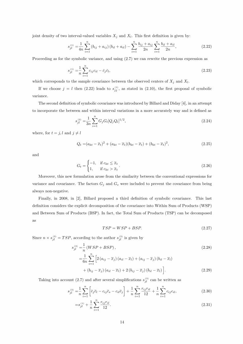
joint density of two interval-valued variables Xj and Xl. This first definition is given by:
s (1)
jl =1
4n
n∑i=1
(bij + aij) (bil + ail)−n∑
i=1
bij + aij2n
n∑i=1
bil + ail2n
, (2.22)
Proceeding as for the symbolic variance, and using (2.7) we can rewrite the previous expression as
s (1)
jl =1
n
n∑i=1
cijcil − cj cl, (2.23)
which corresponds to the sample covariance between the observed centers of Xj and Xl.
If we choose j = l then (2.22) leads to s (1)
jj , as stated in (2.10), the first proposal of symbolic
variance.
The second definition of symbolic covariance was introduced by Billard and Diday [4], in an attempt
to incorporate the between and within interval variations in a more accurately way and is defined as
s (2)
jl =1
3n
n∑i=1
GjGl[QjQl]1/2, (2.24)
where, for t = j, l and j 6= l
Qt =(akt − xt)2 + (akt − xt)(bkt − xt) + (bkt − xt)2, (2.25)
and
Gt =
{−1, if ckt ≤ xt1, if ckt > xt
. (2.26)
Moreover, this new formulation arose from the similarity between the conventional expressions for
variance and covariance. The factors Gj and Gs were included to prevent the covariance from being
always non-negative.
Finally, in 2008, in [2], Billard proposed a third definition of symbolic covariance. This last
definition considers the explicit decomposition of the covariance into Within Sum of Products (WSP)
and Between Sum of Products (BSP). In fact, the Total Sum of Products (TSP) can be decomposed
as
TSP = WSP +BSP. (2.27)
Since n× s (3)
jl = TSP , according to the author s (3)
jl is given by
s (3)
jl =1
n(WSP +BSP ) , (2.28)
=1
6n
n∑i=1
[2 (aij − xj) (ail − xl) + (aij − xj) (bil − xl)
+ (bij − xj) (ail − xl) + 2 (bij − xj) (bil − xl)]. (2.29)
Taking into account (2.7) and after several simplifications s (3)
jl can be written as
s (3)
jl =1
n
n∑i=1
[cjcl − cijcs − cilcj
]+
1
n
n∑i=1
rijril12
+1
n
n∑i=1
cijcil, (2.30)
=s (1)
jl +1
n
n∑i=1
rijril12
. (2.31)
14
Note that if in (2.31) we consider l = j, then we obtain the third definition of symbolic covariance,
which is the desirable property. In some sense, the symbolic covariance of some interval-valued variable
with itself is its symbolic variance, according to the proper definition of symbolic variance.
Thus, like before, if we consider data as realizations of sequences of random vectors:
(Ci1, . . . , Cip, Ri1, . . . , Rip)t with finite variances, Var(Cj) and Var(Rj), j = 1, . . . p, then by the weak
law of large numbers, for j 6= l, we have that:
S (1)
jl =1
n
n∑i=1
CijCil − CjClp−→ Cov(Cj , Cl), (2.32)
S (3)
jl =S (1)
jl +1
n
n∑i=1
RijRil
12
p−→ Cov(Cj , Cl) +1
12E(RjRl). (2.33)
The convergence results obtained by the weak law of large numbers allow writing the several
versions of symbolic covariance matrices as a function of Var(C), Var(R), and Cov(C,R), as stated
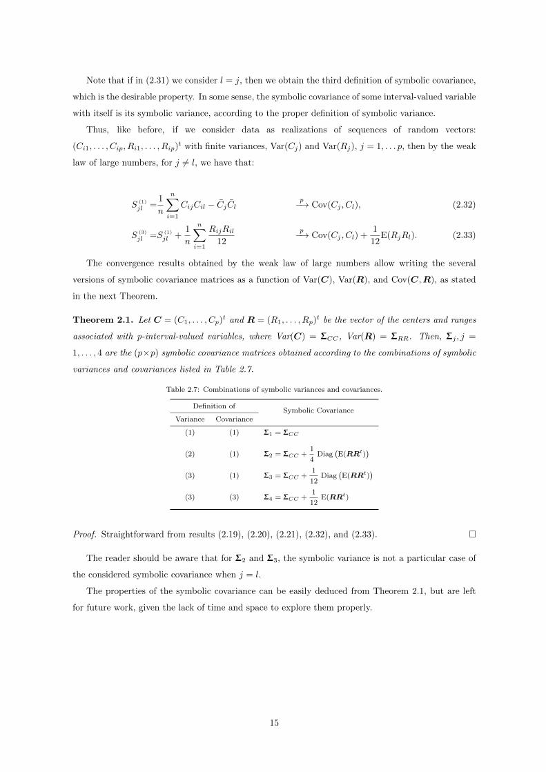
in the next Theorem.
Theorem 2.1. Let C = (C1, . . . , Cp)t and R = (R1, . . . , Rp)t be the vector of the centers and ranges
associated with p-interval-valued variables, where Var(C) = ΣCC , Var(R) = ΣRR. Then, Σj , j =
1, . . . , 4 are the (p×p) symbolic covariance matrices obtained according to the combinations of symbolic
variances and covariances listed in Table 2.7.
Table 2.7: Combinations of symbolic variances and covariances.
Definition ofSymbolic Covariance
Variance Covariance
(1) (1) Σ1 = ΣCC
(2) (1) Σ2 = ΣCC +1
4Diag
(E(RRt)
)(3) (1) Σ3 = ΣCC +
1
12Diag
(E(RRt)
)(3) (3) Σ4 = ΣCC +
1
12E(RRt)
Proof. Straightforward from results (2.19), (2.20), (2.21), (2.32), and (2.33).
The reader should be aware that for Σ2 and Σ3, the symbolic variance is not a particular case of
the considered symbolic covariance when j = l.
The properties of the symbolic covariance can be easily deduced from Theorem 2.1, but are left
for future work, given the lack of time and space to explore them properly.
15
Chapter 3
Symbolic Principal ComponentAnalysis
3.1 Introduction
In the conventional framework, one of the main uses of Principal Components Analysis (PCA) is as a
dimension reduction methodology. The key idea behind this methodology is to find linear combinations
of the original variables whose weights are orthogonal to each other, with unitary norm that maximize
the variance of the new variables. These restrictions lead to new uncorrelated variables, called principal
components, PC, that preserve the total (and generalized) variance of the original variables. Moreover,
it can be proved [35] that the weights defining the PCs, γi, are the eigenvectors of Σ, the covariance
matrix of the original variables, X = (X1, . . . , Xp)t. This can be summarized by
PCi =γti(X − µ), i = 1, . . . p (3.1)
such that
γ1 = argmaxγ:‖γ‖=1
Var(γt(X − µ)
)and
γi = argmaxγ:‖γ‖=1∧γtγk=0
k=1,...i−1
Var(γt(X − µ)
), i = 2, . . . p
Since the obtained PCs depend on the scales at which the variables are measured, variables with
the highest sample variances tend to dominate the first PCs. In general, if the variables are measured
on scales with different magnitudes or different units, they should be standardized before applying
PCA. In this case, the PCs are obtained from the eigenvectors of the correlation matrix.
It should be noted that the determination of these components is frequently used as an intermediate
step in the analysis of complex problems [35], being used as input to others multivariate methods.
Moreover, this is a widely used method because of the frequent need to perform dimension reduction
and PCs are easily estimated and the underlying concepts behind this method are in general simple.
16

Due to this popularity and acknowledged benefits, in recent years several approaches have been
proposed to extend this methodology to the SDA framework, namely to interval-valued variables.
The methods CPCA (centers) and VPCA (vertices), pioneers in symbolic PCA, were proposed
in [10], and are the best known examples of this family of methods. However, recently many other
alternatives have emerged in the literature (vide e.g. [38, 59]).
In Table 3.1 we present the most known SPC methods proposed for interval-valued data until
this moment. The SPC methods can be divided in three groups, according to the strategy type:
(i) symbolic-conventional-symbolic , (ii) symbolic-symbolic-symbolic, and (iii) hybrid. The first, and
most popular, type considers symbolic data, transforms it into conventional, applies conventional PCA
and finally transforms it into symbolic representation. The second type considers all the analysis in
a symbolic framework and the third type considers input and output symbolic but in between uses
conventional linear combinations and interval algebra.
Table 3.1: Symbolic principal component estimation methods - Type of strategy.
Reference Year Method Input - Type - Output
[10] 1997 CPCA (Centers) symbolic-conventional-symbolic[10] 1997 VPCA (Vertices) symbolic-conventional-symbolic[36] 200 SO-PCA symbolic-conventional-symbolic
RT-PCA symbolic-conventional-symbolicSO-PCA Mix symbolic-conventional-symbolic
[45] 2003 Midpoints and radii PCA hybrid[27] 2006 IPCA symbolic-symbolic-symbolic[59] 2012 CIPCA symbolic-conventional-symbolic[38] 2012 Symbolic Covariance PCA symbolic-conventional-symbolic
One common aspect that these SPC methods share is the fact that they are all described by
thorough algorithms, that most times require demanding computation time and complexity. In this
sense, when we analysed these methods our main concern was the lack of a population formulation.
And, for instance, in simulation studies, the results are usually compared with the “best” known
method, traditionally VPCA and CPCA. However, we argue that this is not the correct approach
since it may lead to biased conclusions. Moreover, we think that the theoretical properties of the
SPC are not clear and it is essential to discuss which known properties of conventional PCA still
remain valid and if the definitions of basic statistical concepts is still so straightforward. We have the
insight that all these difficulties, combined with the novelty of the symbolic approach, may discourage
the use of SPCA to analyse real data outside the symbolic community. Therefore, in this thesis and
in particular in this chapter we review the current SPCA methods and analyse some of them with
the purpose of clarifying the underlying concepts and properties. Additionally, we also discuss some
possible techniques used to define and represent the SPC scores.
It should be noted that the original formulations of most of the methods addressed in this chapter
were presented in terms of the correlation matrix. However, here we only present versions based on
the covariance matrix because we consider that this is the most general formulation.
17

3.2 SPCA Methods
First of all, it is necessary to define the input matrix that will be used as the starting point for most
of the methods reviewed in this section. Thus, from Chapter 2, we can define an interval-valued data
matrix summarizing the macro-data characterizing n objects or entities, described by p interval-valued
variables as a (n× p) matrix which presents the following format:
ξ =
[a11, b11] [a12, b12] · · · [a1p, b1p]
[a21, b21] [a22, b22] · · · [a2p, b2p]
......
. . ....
[an1, bn1] [an2, bn2] · · · [anp, bnp]
, (3.2)
where aij ≤ bij , for all i = 1, 2, . . . , n and j = 1, 2, . . . p.
This matrix can be rewritten in terms of centers and ranges using (2.1) and (2.2), resulting in:
ξ =
[c11 −
r11
2, c11 +
r11
2
] [c12 −
r12
2, c12 +
r12
2
]· · ·
[c1p −
r1p
2, c11 +
r1p
2
][c21 −
r21
2, c21 +
r21
2
] [c22 −
r22
2, c22 +
r22
2
]· · ·
[c2p −
r2p
2, c2p +
r2p
2
]...
.... . .
...[cn1 −
rn1
2, cn1 +
rn1
2
] [cn2 −
rn2
2, cn2 +
rn2
2
]· · ·
[cnp −
rnp2, cnp +
rnp2
]
. (3.3)
Moreover, since most of the methods addressed here are based on the symbolic-conventional-
symbolic strategy it is also useful to define the associated matrices of centers and ranges, respectively
C =
c11 c12 · · · c1pc21 c22 · · · c2p...
.... . .
...cn1 cn2 · · · cnp
, (3.4)
R =
r11 r12 · · · r1p
r21 r22 · · · r2p
......
. . ....
rn1 rn2 · · · rnp
. (3.5)
In what follows, we review the methodologies displayed in Table 3.1 and for four of them, namely
the first methods introduced, CPCA and VPCA (Cazes et al. [10]) and two of the more recent propos-
als, Complete Information PCA (Wang et al. [59]), and Symbolic Covariance PCA (Le-Rademacher
and Billard [38]), we present population formulations that allow defining a general and a computa-
tionally more efficient proceeding to implement these methods.
18
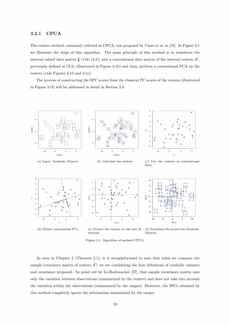
3.2.1 CPCA
The centers method, commonly referred as CPCA, was proposed by Cazes et al. in [10]. In Figure 3.1
we illustrate the steps of this algorithm. The main principle of this method is to transform the
interval-valued data matrix ξ (vide (3.2)) into a conventional data matrix of the interval centers, C,
previously defined in (3.4) (illustrated in Figure 3.1b) and then, perform a conventional PCA on the
centers (vide Figures 3.1d and 3.1e).
The process of constructing the SPC scores from the classical PC scores of the centers (illustrated
in Figure 3.1f) will be addressed in detail in Section 3.4.
−10 −5 0 5
−5
05
Variable 1
Var
iabl
e 2
(a) Input: Symbolic Objects.
−10 −5 0 5
−5
05
Variable 1
Var
iabl
e 2
●
●
●
●
●
●
●●
●
●
●
●
●
●
●
●●
●
●
●
●
●
●
●
●
●
●
●
●
●
●
●
●
●
●
(b) Calculate the centers.
●
●
●
●
●
●
●●
●
●
●
●
●
●
●
●●
●
●
●
●
●
●
●
●
●
●
●
●
●
●
●
●
●
●
−10 −5 0 5−
6−
4−
20
24
68
C 1
C 2
(c) Use the centers as conventionaldata.
●
●
●
●
●
●
●●
●
●
●
●
●
●
●
●●
●
●
●
●
●
●
●
●
●
●
●
●
●
●
●
●
●
●
−10 −5 0 5
−6
−4
−2
02
46
8
C 1
C 2
(d) Obtain conventional PCs.
●
●
●
●
●
●
●
●
●
●
●
●
●
●
●
●
●
●
●
●
●
●
●
●
●
●
●
●
●
●
●
●
●
●
●
−5 0 5 10
−6
−4
−2
02
4
PCA 1
PC
A 2
(e) Project the centers on the new di-rections.
−10 −5 0 5 10
−6
−4
−2
02
46
PC 1
PC
2
(f) Transform the scores into SymbolicObjects.
Figure 3.1: Algorithm of method CPCA.
As seen in Chapter 2 (Theorem 2.1), it is straightforward to note that when we compute the
sample covariance matrix of centers, C, we are considering the first definitions of symbolic variance
and covariance proposed. As point out by Le-Rademacher [37], that sample covariance matrix uses
only the variation between observations (summarized by the centers) and does not take into account
the variation within the observations (summarized by the ranges). Moreover, the SPCs obtained by
this method completely ignore the information summarized by the ranges.
19

3.2.2 VPCA
Along with the previous method, the vertices method was also proposed by Cazes et al. in [10] and
follows similar basic principles. As the name suggests, the VPCA method is based on the vertices of
the hyper-rectangles associated with each observation. In Figure 3.2 we illustrate the main steps of this
algorithm. First, transforming the interval-valued data matrix ξ (vide (3.2)) into a conventional data
matrix of the interval vertices, V , whose details description is done below. Then (vide Figure 3.2c),
perform a conventional PCA on the vertices matrix (Figures 3.2d and 3.2e). Finally, the algorithm
constructs the SPC scores from the classical PC scores of the vertices. The algorithm to do this
conversion is discussed in detail in Section 3.4.
−10 −5 0 5
−5
05
Variable 1
Var
iabl
e 2
(a) Input: Symbolic Objects.
−10 −5 0 5
−5
05
Variable 1
Var
iabl
e 2
●
●
●
●
●
●
●●
●
●
●
●
●
●
●
●●
●
●
●
●
●
●
●
●
●
●
●
●
●
●
●
●
●
●
●
●
●
●
●
●
●●
●
●
●
●
●
●
●
●●
●
●
●
●
●
●
●
●
●
●
●
●
●●
●
●
●
●
●
●
●
●
●
●
●●
●
●
●
●
●
●
●
●●
●
●
●
●
●
●
●
●
●
●
●
●
●●
●
●
●
●
●
●
●
●
●
●
●●
●
●
●
●
●
●
●
●●
●
●
●
●
●
●
●
●
●
●
●
●
●
●
●
●
●
●
(b) Calculate the vertices.
−10 −5 0 5
−5
05
Variable 1
Var
iabl
e 2
●
●
●
●
●
●
●●
●
●
●
●
●
●
●
●●
●
●
●
●
●
●
●
●
●
●
●
●
●
●
●
●
●
●
●
●
●
●
●
●
●●
●
●
●
●
●
●
●
●●
●
●
●
●
●
●
●
●
●
●
●
●
●●
●
●
●
●
●
●
●
●
●
●
●●
●
●
●
●
●
●
●
●●
●
●
●
●
●
●
●
●
●
●
●
●
●●
●
●
●
●
●
●
●
●
●
●
●●
●
●
●
●
●
●
●
●●
●
●
●
●
●
●
●
●
●
●
●
●
●
●
●
●
●
●
(c) Use the vertices as conventionaldata.
−10 −5 0 5
−5
05
Variable 1
Var
iabl
e 2
●
●
●
●
●
●
●●
●
●
●
●
●
●
●
●●
●
●
●
●
●
●
●
●
●
●
●
●
●
●
●
●
●
●
●
●
●
●
●
●
●●
●
●
●
●
●
●
●
●●
●
●
●
●
●
●
●
●
●
●
●
●
●●
●
●
●
●
●
●
●
●
●
●
●●
●
●
●
●
●
●
●
●●
●
●
●
●
●
●
●
●
●
●
●
●
●●
●
●
●
●
●
●
●
●
●
●
●●
●
●
●
●
●
●
●
●●
●
●
●
●
●
●
●
●
●
●
●
●
●
●
●
●
●
●
(d) Obtain conventional PCs.
−5 0 5 10
−6
−4
−2
02
46
PCA 1
PC
A 2
●
●
●
●
●
●
●
●
●
●
●
●
●
●
●
●
●
●
●
●
●
●
●
●
●
●
●
●
●
●
●
●
●
●
●
●
●
●
●
●
●
●
●
●
●
●
●
●
●
●
●
●
●
●
●
●
●
●
●
●
●
●
●
●
●
●
●
●
●
●
●
●
●
●
●
●
●
●
●
●
●
●●
●
●
●
●
●
●
●
●
●
●
●
●
●
●
●
●
●
●
●
●
●
●
●
●
●
●
●
●
●
●
●
●
●
●
●
●
●
●
●
●
●
●
●
●
●
●
●
●
●
●
●
●
●
●
●
●
●
(e) Project the vertices on the new di-rections.
−10 −5 0 5 10
−6
−4
−2
02
46
PC 1
PC
2
(f) Transform the scores into SymbolicObjects.
Figure 3.2: Algorithm of method VPCA.
This algorithm requires the construction of the matrix of vertices. Considering the interval-valued
matrix ξ, defined in (3.3), the ith observation
ξi =([ci1 −
ri12, ci1 +
ri12
], . . . ,
[cip −
rip2, cip +
rip2
])tcan be associated with the ith hyper-rectangle, which has 2qi vertices, where qi is the number of
non-trivial intervals (see Figure 2.2). Thus, this hyper-rectangle can be represented by an (2qi × p)
matrix V i. And finally, the (n∑
i=1
2qi × p) matrix of the vertices associated with all observations, V , is
20

defined as follows:
V =
V 1
...V n
=
c11 −
r11
2· · · c1q1 −
r1q1
2...
. . ....
c11 +r11
2· · · c1q1 +
r1q1
2
...
cn1 −rn1
2· · · cnqn −
rnqn2
.... . .
...
cn1 +rn1
2· · · cnqn +
rnqn2
. (3.6)
For example, in a dataset with p = 2 symbolic variables, each symbolic object is identified by four
vertices, presented as red dots in Figure 3.3. As seen before, the observation
ξi =([ci1 −
ci12, ci1 +
ci12
],[ci2 −
ci22, ci2 +
ci22
])t,
can be represented by the matrix V i:
V i =
ci1 −ri12
ciqi −riqi2
ci1 −ri12
ciqi +riqi2
ci1 +ri12
ciqi −riqi2
ci1 +ri12
ciqi +riqi2
. (3.7)
Figure 3.3: Representation of a symbolic object with p = 2 symbolic variables.
In general, the original sample of dimension n leads to a new sample of dimension 2pn (if there
are no trivial intervals), which will be used as input for the conventional PCA.
21

This formulation can be rewritten to show that the covariance matrix based on which we construct
the VPCA symbolic PCs can be defined as a function of the first and second moments of the centers
and ranges.
Let us consider that all the observed interval-valued variables are non-trivial, i.e. aij < bij , thus
qi = p for i = 1, . . . , n and V is a (2pn× p) matrix.
Given the ith object described by (ci1, . . . , cip, ri1, . . . , rip)t, the 2p vertices, characterizing the
associated hyper-rectangle can be written as{(wi11, . . . , wip1) , . . . , (wi12p , . . . , wip2p) , i = 1, . . . , n
}, (3.8)
where wijk represents the kth vertex coordinate describing the ith object, on the jth symbolic variable,
i = 1, . . . , n, j = 1, . . . , p, k = 1, . . . , 2p. Using a similar notation of the construction of V i, this list
can be written as:{(ci1 −
ri12, . . . , cp1 −
rp1
2
), . . . ,
(ci1 +
ri12, . . . , cp1 +
rp1
2
), i = 1, . . . , n
}. (3.9)
Then, the sample mean associated with the jth coordinate of all vertices is:
wj =1
2pn
n∑i=1
2p∑k=1
wijk, j = 1, . . . , p. (3.10)
Due to the symmetry of the problem, for each object half of the vertices are equal to cij − rij2 and
the others to cij +rij2 . So, the 2p summands over k can be rearranged in two parts:
wj =1
n
1
2p
2p−1∑k=1
(cij −
rij2
)+
1
2p
2p−1∑k=1
(cij +
rij2
) , (3.11)
Then, after some simplifications it can easily be shown that
wj =1
n
n∑i=1
cij = cj , (3.12)
The sample variance of jth coordinate of a vertex, based on (3.8) can be obtained as:
s (W )
jj =1
2pn
n∑i=1
2p∑k=1
(wijk − wj)2, (3.13)
as usually, we can write
s (W )
jj =1
2pn
(n∑
i=1
2p∑k=1
w2ijk − 2pnw2
j
). (3.14)
Once again, due to the symmetry of the problem each vertex can be rewritten in terms of centers
and ranges, leading to
s (W )
jj =1
2pn
(2p−1
n∑i=1
(cij −
rij2
)2
+ 2p−1n∑
i=1
(cij +
rij2
)2
− 2pn c2j
),
=1
n
n∑i=1
c2ij − c2j +1
n
n∑i=1
r2ij
4. (3.15)
22

Like before, the sample covariance between the jth and lth vertex coordinate is given by:
s (W )
jl =1
2pn
n∑i=1
2p∑k=1
(wijk − wj) (wilk − wl) . (3.16)
Similarly to the variance, the covariance can also be expressed in terms of centers and ranges as
s (W )
jl =1
2pn
(2p−2
n∑i=1
(cij −
rij2
)(cij +
rij2
)+ 2p−2
n∑i=1
(cij +
rij2
)(cij −
rij2
)+ 2p−2
n∑i=1
(cij −
rij2
)2
+ 2p−2n∑
i=1
(cij +
rij2
)2
− 2pn cj cl
),
=1
n
n∑i=1
cijcil − cj cl. (3.17)
Finally, if cij and rij , i = 1, . . . , n are considered realizations of sequences of random vectors:
(Ci1, . . . , Cip, Ri1, . . . , Rip)t with finite variances, Var(Cj) and Var(Rj), j = 1, . . . p, then the weak
law of large numbers guarantees that:
Wjp−→ E(Cj), (3.18)
S (W )
jj
p−→ Var(Cj) +1
4E(R2
j ), (3.19)
S (W )
jl
p−→ Cov(Cj , Cl), (3.20)
for j, l = 1, . . . , p with j 6= l, where
Wj = Cj ,
S (W )
jj =1
n
n∑i=1
C2ij − C2
j +1
n
n∑i=1
R2ij
4,
and
S (W )
jl =1
n
n∑i=1
CijCil − CjCl.
So, we have proved that the covariance matrix of the vertices used in the VPCA method, SVPCA
converges to
ΣVPCA = ΣCC +1
4Diag
(E(RRt)
), (3.21)
which corresponds to the second symbolic covariance matrix, Σ2, defined in Theorem 2.1.
This result written as function of the sample quantities was previously proved by Douzal-Chouakria
et al. in [22] (vide pag. 14) and, in some sense, also presented in [59] (vide pag. 164), but was not
formulated in this form. The authors obtained the same decomposition for the covariance matrix of
the vertices recognizing that one of the components represents the variation between the centers of
the observations and the other the interval variation within each observation.
Thus, the VPCA method is an improvement over CPCA, since using the vertices allows consid-
ering some of the internal variation of the observations as proved by Douzal-Chouakria et al. in [22].
However, in some sense, this method treats the vertices as independent observations and this is not
true, in fact the vertices of a hyper-rectangle are not independent.
23
3.2.3 SO-PCA: mixed Strategy
As previously discussed, VPCA ignores that the vertices of a certain hyper-rectangle are dependent
observations. Motivated by this fact, Lauro and Palumbo [36] proposed three approaches in a attempt
to improve VPCA incorporating the dependency among vertices of the same observation. The first ap-
proach, called symbolic-object PCA (SO-PCA), is an adaptation of the method VPCA by introducing
a boolean matrix B, where for q = 1 . . . , n2p (if there are no degenerate variables) and i = 1 . . . , n:
Bqi =
1, if the qth vertex belongs to the ith observation
0, otherwise,
(3.22)
The procedure consists in obtaining the pairs (λVk ,uVk ) for the matrix
1
N(ZV )tB(BtB)−1BtZV
where ZV is the standardised version of the matrix of vertices V , defined in (3.6) and N = n2p is the
number of rows of B. Then, the SPC scores are obtained as for CPCA, and like in that case it only
accounts for the variation between observations.
The second procedure, range-transformation PCA (RT-PCA), is an attempt to also account for
the internal structure of interval-valued observations and uses only the range of the intervals. The
transformation applied moves the hyper-rectangles in a way that the vertices close to the origin are
shifted over there. This method consists in determining the matrix of the ranges R, defined by (3.5)
and then apply conventional PCA.
This method is mainly focused in analysing the size and shape of the symbolic observations. So,
if this is the only purpose of our analysis the method can be used alone, otherwise we can follow a
third approach of [36], based on the combination of SO-PCA and RT-PCA. This mixed strategy can
be summarized in three steps:
• Apply the method RT-PCA to extract the PCs that better represent the size and shape of the
symbolic objects, T ;
• Transform ZV into Z∗ = B(BtB)−1BtZV (method SO-PCA);
• Apply conventional PCA on P TZ∗, where P T is a projection matrix of T .
This last proposal has several drawbacks, inherited from the other two approaches, namely: the
matrix calculations involved are computationally heavy, the results rely on the choice of the RT-PCA
(sub)space and cannot be applied to observations with identical shape and size, i.e., if the majority
of the observations have the same range.
3.2.4 Midpoints and radii PCA
The method Midpoints and radii principal component analysis (MRPCA) was also proposed by
Palumbo and Lauro [45]. This methodology follows a hybrid strategy since it takes advantage of
the techniques of interval algebra and linear algebra. According to this proposal, conventional PCA
can be applied to either the midpoints or the midranges of the intervals. That is, we can obtain the
24

matrix of centers, C (see (3.4)) or the matrix of the midranges,1
2R (see (3.5)) and perform con-
ventional PCA. These two approaches have the same disadvantages as SO-PCA and RT-PCA. In an
attempt to take into account both the centers and the midranges they proposed a new approach by
superimposing the PCs of the midranges onto the PCs of the centers and then rotate the midranges,
using Procrustes rotation, in order to maximize the connection between both elements. Then, the
SPC scores can be obtained by the reconstruction formula, as follows:
SPCik =[PCC
ik − PCCRik ,PCC
ik + PCCRik
], (3.23)
where PCC and PCCR are the conventional PC scores of the centers and the rotated midranges.
Several authors have pointed out the drawbacks of this method, for instance Lauro, Verde, and
Irpino in Chapter 15 of [18] argued that the choice of the rotation operator is subjective and despite
this rotation the method still treats the center and the midrange as two separate variables, which does
not reflect the correct structure behind an interval-valued variable.
3.2.5 Interval PCA
In 2006, Gioia and Lauro [27] proposed a methodology named Interval Principal Component Analysis
(IPCA). This is the only method that follows the symbolic–symbolic–symbolic strategy and it is mainly
based on interval linear algebra, introduced by Moore [42].
The initial approach of this method is described as follows. Given an interval-valued data matrix
ξ as defined in (3.3), we obtain the PCs of ξ (centered) by solving this interval eigenvalue problem:
ξtξuIk = λIk, (3.24)
which, for k = 1, . . . , p has the following interval solutions
λIk ={λ : Zu = λu,∀Z ∈ ξtξ
}, (3.25)
uIk =
{u : Zu = λu,∀Z ∈ ξtξ
}. (3.26)
These solutions are, respectively, the sets of all kth eigenvalues and eigenvectors obtained from all the
real-valued matrices Z ∈ ξtξ, where ξtξ is defined as the product interval matrix (vide Definition
2.2.3 in [27]:
ξtξ ={UW : U ∈ ξt,W ∈ ξ
}. (3.27)
However, with his formulation the PCs obtained are oversized with respect to the real solution. In
particular, Gioia and Lauro [27] observed that
ξtξ ⊃{U tU : U ∈ ξ
}, (3.28)
which means that the set ξtξ also contains matrices that are not of the desirable form: U tU . To
overcome this drawback, they proposed the reformulation of the eigenvalue problem considering a new
set of matrices,
Θt ={U tU : U ∈ ξt
}, (3.29)
25

instead of the product interval matrix ξtξ.
The main disadvantage of this method is the fact that finding these interval solutions is a problem
computationally hard. Moreover, the authors of this method also underline that the exact bounds can
only be found for small intervals, in particular with intervals where the ratio between the half-range
and the center of the interval is approximately of 2-3%. For those reasons, this method will not be
further addressed in this thesis.
3.2.6 Complete Information PCA
In [59], Wang and co-authors argue that the SPCs obtained in CPCA and VPCA only reflect the
structure of the centers and the vertices of the hyper-rectangles. In a attempt to incorporate the com-
plete information inside the hyper-rectangles, they proposed a new method, the Complete Information
PCA method (CIPCA).
This approach is mainly based on the definition of the inner product and the squared norm opera-
tors for interval-valued data. In particular, given two interval-valued variables Xj and Xl, with j 6= l
(see Definition 2.1), its inner product is defined as
⟨Xj , Xl
⟩=
n∑i=1
〈xij , xil 〉, (3.30)
where
〈xij , xil 〉 =
∫ bil
ail
∫ bij
aij
st1
(bij − aij)(bil − ail)ds dt, (3.31)
=1
4(aij + bij)(ail + bil). (3.32)
And for an interval-valued variable Xj , the squared norm is given by
‖Xj‖2 =
n∑i=1
‖xj‖2, (3.33)
where
‖xj‖2 =
∫ bij
aij
s2 1
(bij − aij)ds, (3.34)
=1
3(a2
ij + aijbij + b2ij). (3.35)
It is important to note that ‖Xj‖2 6= 〈Xj , Xj 〉. Moreover, the covariance matrix considered in this
method is computed by defining:
CovCIPCA(Xj , Xl) =1
n
⟨Xj , Xl
⟩=
n∑i=1
1
4n(aij + bij)(ail + bil), j 6= l (3.36)
and
VarCIPCA(Xj) =1
n‖Xj‖2 =
n∑i=1
1
3n(a2
ij + aijbij + b2ij). (3.37)
26

Then, we obtain the spectral decomposition of the covariance matrix, as in the conventional case.
Finally, we transform the conventional PC scores into SPC scores.
In [59], the authors noticed that the covariance matrices considered in the methods CPCA, VPCA,
and CIPCA, have the same off diagonal elements and that for the symbolic variances the following
inequality holds:
VarCPCA(Xj) ≤ VarCIPCA(Xj) ≤ VarVPCA(Xj). (3.38)
They established this inequality by proving that
VarVPCA(Xj)−VarCIPCA(Xj) =1
6n
n∑i=1
(bij − aij)2 ≥ 0, (3.39)
VarCIPCA(Xj)−VarCPCA(Xj) =1
12n
n∑i=1
(bij − aij)2 ≥ 0. (3.40)
Wang and co-authors only pointed out that the gap between VarVPCA(Xj) and VarCIPCA(Xj) is
greater than the one between VarCPCA(Xj) and VarCIPCA(Xj) and verified this inequality in a sim-
ulation study. This result motivated us to further explore this method in an attempt to develop a
general formulation that could embrace several methods, in particular these three.
Then, similarly as before, we can rewrite (3.36) and (3.37) in terms of centers and ranges, leading
to
CovCIPCA(Xj , Xl) =1
n
n∑i=1
cijcil − cj cl, j 6= l (3.41)
and
VarCIPCA(Xj) =1
n
n∑i=1
c2ij − c2j +1
n
n∑i=1
r2ij
12. (3.42)
Finally, if (ci1, . . . , cip, ri1, . . . , rip)t , i = 1, . . . , n are considered realizations of sequences of random
vectors: (Ci1, . . . , Cip, Ri1, . . . , Rip)t with finite variances, Var(Cj) and Var(Rj), j = 1, . . . p,, then by
the weak law of large numbers we have that:
VarCIPCA(Xj)p−→ Var(Cj) +
1
12E(R2
j ), (3.43)
CovCIPCA(Xj , Xl)p−→ Cov(Cj , Cl), (3.44)
for j, l = 1, . . . , p with j 6= l.
Hence, we have proved that the covariance matrix associated with CIPCA converges to
ΣCIPCA = ΣCC +1
12Diag
(E(RRt)
), (3.45)
which corresponds to the third symbolic covariance matrix, Σ3, defined in Theorem 2.1.
27

3.2.7 Symbolic Covariance PCA
The Symbolic Covariance PCA method, here referred as SymCovPCA, was proposed by Le-Rademacher
and Billard [38], and along with CIPCA is one of the more recent proposals in SPCA for interval-
valued data. This method is based on the direct computation of a symbolic covariance matrix for
the interval data matrix ξ. In the first version of this method [37], the symbolic covariance matrix
was defined using the third definition for the symbolic variance, S (3)
jj and the second definition for the
symbolic covariance, S (2)
jl , introduced in Chapter 2. However, Billard [2] proposed a more straightfor-
ward definition for the symbolic covariance, namely S (3)
jl , so the method was updated by considering
this new definition instead. Therefore, the current version is based on the fourth symbolic covariance
matrix, Σ4, defined in Theorem 2.1, in terms of centers and ranges as
ΣSymbCovPCA = ΣCC +1
12E(RRt). (3.46)
Thus, the procedure of this method can be summarized in the following steps:
1. Compute the (p× p) symbolic sample covariance matrix, SSymbCovPCA using sample versions of
(3.46);
2. Obtain the spectral decomposition of SSymbCovPCA, as in the conventional case;
3. Transform the conventional PC scores into SPC scores.
Le-Rademacher and Billard [38] proposed a new method to transform the conventional scores into
symbolic. This proposal, based on polytopes theory, is briefly discussed in Section 3.4.
28
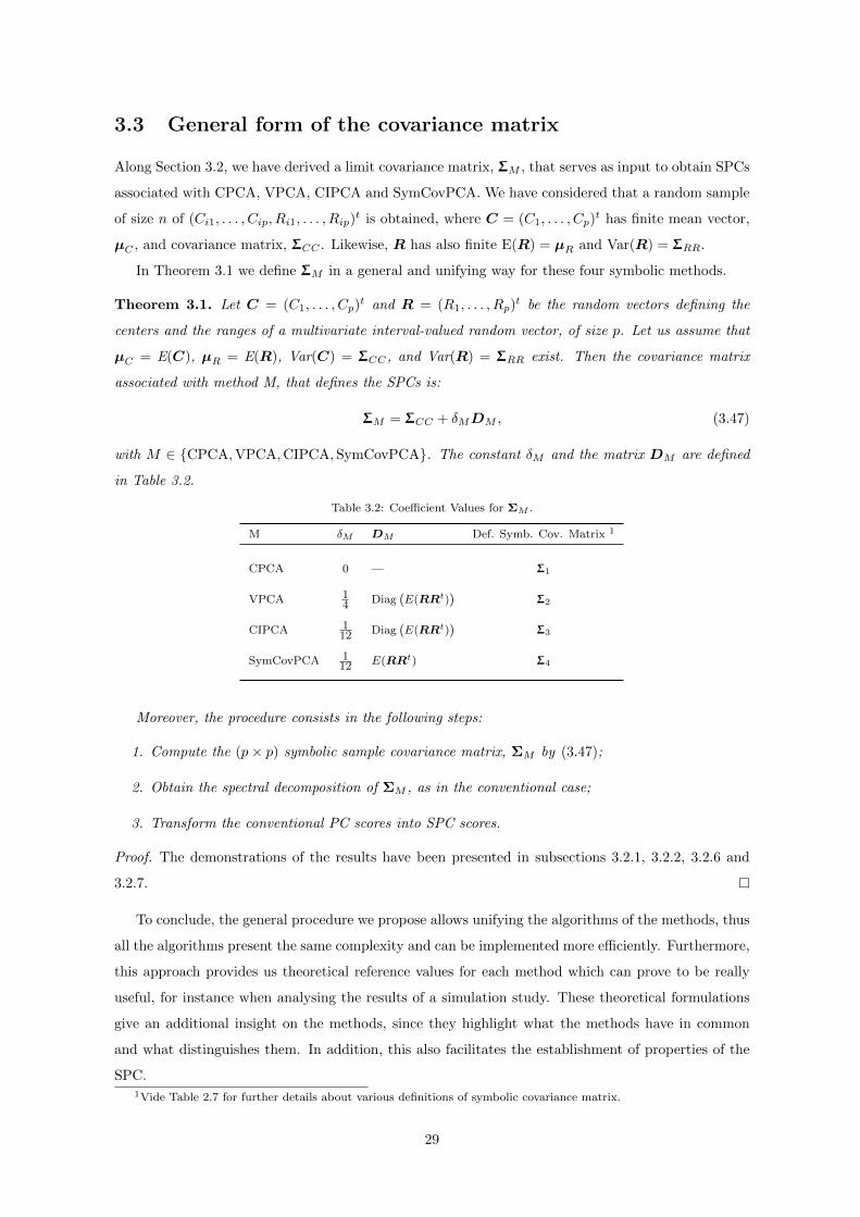
3.3 General form of the covariance matrix
Along Section 3.2, we have derived a limit covariance matrix, ΣM , that serves as input to obtain SPCs
associated with CPCA, VPCA, CIPCA and SymCovPCA. We have considered that a random sample
of size n of (Ci1, . . . , Cip, Ri1, . . . , Rip)t is obtained, where C = (C1, . . . , Cp)t has finite mean vector,
µC , and covariance matrix, ΣCC . Likewise, R has also finite E(R) = µR and Var(R) = ΣRR.
In Theorem 3.1 we define ΣM in a general and unifying way for these four symbolic methods.
Theorem 3.1. Let C = (C1, . . . , Cp)t and R = (R1, . . . , Rp)t be the random vectors defining the
centers and the ranges of a multivariate interval-valued random vector, of size p. Let us assume that
µC = E(C), µR = E(R), Var(C) = ΣCC , and Var(R) = ΣRR exist. Then the covariance matrix
associated with method M, that defines the SPCs is:
ΣM = ΣCC + δMDM , (3.47)
with M ∈ {CPCA,VPCA,CIPCA,SymCovPCA}. The constant δM and the matrix DM are defined
in Table 3.2.
Table 3.2: Coefficient Values for ΣM .
M δM DM Def. Symb. Cov. Matrix 1
CPCA 0 — Σ1
VPCA 14 Diag
(E(RRt)
)Σ2
CIPCA 112 Diag
(E(RRt)
)Σ3
SymCovPCA 112 E(RRt) Σ4
Moreover, the procedure consists in the following steps:
1. Compute the (p× p) symbolic sample covariance matrix, ΣM by (3.47);
2. Obtain the spectral decomposition of ΣM , as in the conventional case;
3. Transform the conventional PC scores into SPC scores.
Proof. The demonstrations of the results have been presented in subsections 3.2.1, 3.2.2, 3.2.6 and
3.2.7.
To conclude, the general procedure we propose allows unifying the algorithms of the methods, thus
all the algorithms present the same complexity and can be implemented more efficiently. Furthermore,
this approach provides us theoretical reference values for each method which can prove to be really
useful, for instance when analysing the results of a simulation study. These theoretical formulations
give an additional insight on the methods, since they highlight what the methods have in common
and what distinguishes them. In addition, this also facilitates the establishment of properties of the
SPC.1Vide Table 2.7 for further details about various definitions of symbolic covariance matrix.
29

3.4 Representation of Symbolic Scores
Until now, we have analysed how to determine the coefficients of the conventional PCs for each method,
the conventional step of the procedure to define SPCs. Having solved this problem, we have to write
the objects in the space spanned by the new variables, i.e. we have to reconstruct the observations in
the SPC space, called symbolic scores or just scores when there is no doubt of being or not symbolic.
In Table 3.3 we present the type of representation of the scores each author uses in each method. The
most common and simple method is the Maximum Covering Area Rectangle, MCAR, representation,
however, as we will see it also has drawbacks, and limitations.
Table 3.3: Symbolic principal component estimation methods - Type of representation.
Reference Method Representation
[10] Centers (CPCA) MCAR[10] Vertices (VPCA) MCAR[36] SO-PCA MCAR
RT-PCA Size/shape of the SO’s a
SO-PCA Mix MCAR
[45] Midpoints and radii PCA Using a reconstruction formula b
[27] IPCA Using the inner product interval operator[59] CIPCA MCAR[38] Symbolic Covariance PCA Polytopes
a Using the max vertices coordinates.b Based on midpoint and radius rotation operators.
The MCAR representation was introduced by Chouakria [11] to obtain the SPC scores of the
CPCA and VPCA methods. According to this proposal, the kth SPC (centered) score obtained by
the method CPCA is given by
SPCCk (ξi) =SPCC
ik, (3.48)
=[PCC
k (min i),PCCk (max i)
], (3.49)
where k = 1, . . . , p, i = 1, . . . , n and γk is the kth eigenvector of ΣCC . Moreover, the lower bound is
PCCk (min i) =
p∑j=1
minaij≤xij≤bij
(xij − xj)γkj . (3.50)
The author suggested that the score is an interval, where the lower bound is formed by the linear
combinations of the lower bounds of the original interval in case of positive weights, γkj > 0, plus the
combination of the upper bounds if the weights are negative, γkj < 0 , leading to
PCCk (min i) =
p∑j:γkj>0
(aij − xj)γkj +
p∑j:γkj<0
(bij − xj)γkj , (3.51)
where xj =1
n
n∑i=1
aij + bij2
.
The upper bound is
PCCk (max i) =
p∑j=1
maxaij≤xij≤bij
(xij − xj)γkj , (3.52)
=
p∑j:γkj>0
(bij − xj)γkj +
p∑j:γkj<0
(aij − xj)γkj . (3.53)
30

Moreover, for k = 1, . . . p the hyper-rectangle formed by the first k SPCs, (SPCCi1, . . . ,SPCC
ik)t is
the MCAR k-dimensional representation of the ith object.
Taking into account that aij = cij −rij2, bij = cij +
rij2, and xj = cj , we can rewrite the limits as
PCCk (min i) =
p∑j:γkj>0
(cij −
rij2− cj
)|γkj | −
p∑j:γkj<0
(cij +
rij2− cj
)|γkj |, (3.54)
PCCk (max i) =
p∑j:γkj>0
(cij +
rij2− cj
)|γkj | −
p∑j:γkj<0
(cij −
rij2− cj
)|γkj |. (3.55)
Then, after some calculations we can conclude that
SPCCik =
[γtk(ci − c)−
1
2|γk|tri, γt
k(ci − c) +1
2|γk|tri
], (3.56)
where γk is the kth eigenvector of ΣCC , k = 1, . . . , p, |γk| = (|γk1|, . . . , |γkp|)t, ci = (ci1, . . . , cip)t,
ri = (ri1, . . . , rip)t, and c = (c1, . . . , cp)t is the sample mean vector of the centers.
Thus, the representation of the ith object in the kth SPC is an interval whose center is the linear
combination of the (centered) centers γtk(ci− c). The range of the new interval is defined by the linear
combination of the original ranges, having only positive weights, i.e. the weights on absolute value,
are equal to the weights defining the center of the interval, |γtk|.
If we use standardized data, i.e. c∗ij =cij − cj√
scjj, then the result can be formulated as follows
SPCCik =
[etk(SC)−1(ci − µC)− 1
2|ek|t(SC)−1ri, e
tk(SC)−1(ci − µC) +
1
2|ek|t(SC)−1ri
], (3.57)
where ek is the kth eigenvector of the correlation matrix of the centers, k = 1, . . . , p,
|ek| = (|ek1|, . . . , |ekp|)t, ci = (ci1, . . . , cip)t, ri = (ri1, . . . , rip)t, c = (c1, . . . , cp)t is the sample
mean vector of the centers and (SC)−1 = Diag
(1√sc11
, . . . ,1√scpp
)is the inverse of the matrix with
the standard deviations of the centers in the main diagonal.
Next, we consider the construction of SPC scores for the method VPCA, also based on the MCARs
representation. In this case, for a given observation, ξi, the kth SPC score can be obtained as
SPCVk (ξi) =
[minj
PCik.j ,maxj
PCik.j
], (3.58)
where PCik.j is the kth conventional score of the jth vertex for the ith observation.
According to this formulation, to obtain the desired score we need to calculate the conventional PC
scores for all the vertices associated with a given observation.
31
For example, in a dataset with p = 2 interval-valued variables, if all the variables are non-
degenerate, for a given observation we need to compute the following four scores:
PCik.1 = γ1k (ci1 − ri1/2) + γ2k (ci2 − ri2/2) ,
PCik.2 = γ1k (ci1 − ri1/2) + γ2k (ci2 + ri2/2) ,
PCik.3 = γ1k (ci1 + ri1/2) + γ2k (ci2 − ri2/2) ,
PCik.4 = γ1k (ci1 + ri1/2) + γ2k (ci2 + ri2/2) .
Then, use the minimum and the maximum value as the limits to define SPCVik (see (3.58)). For a
generic number p of interval-valued variables we have to compute the 2p scores, which for large values
of p becomes a really demanding task.
Nevertheless, Douzal-Chouakria et al. in [22] showed that the limits of the SPC scores in (3.58)
can be obtained like the limits of the SPC scores for CPCA (see (3.51) and (3.53)).
This is a particularly useful result since, along with the population formulation we deduced for
the VPCA method, it allows applying the method and representing the SPC scores without having
to compute de vertices matrix, thus reducing the complexity of the algorithm.
As we saw in Table 3.3, almost all the methods based on the strategy symbolic–conventional-
symbolic use the MCARs to construct the SPC scores from the conventional PC scores. So, we state
here a more general result we have deduced, using the same procedure as exemplified for the centers.
Theorem 3.2. Let C = (C1, . . . , Cp)t and R = (R1, . . . , Rp)t be the random vectors of the centers
and the ranges describing an interval-valued population of size p, such that: µC = E(C), µR = E(R),
Var(C) = ΣCC , and Var(R) = ΣRR exist.
Let ΣM be the matrix associated with a given symbolic-conventional-method M,
(M ∈ {CPCA, VPCA, CIPCA, SymCovPCA}), and (λ1,γ1), . . . , (λp,γp) be the eigenvalue-eigenvector
pairs of ΣM , such that λ1 ≥ λ2 ≥ . . . ≥ λp ≥ 0. Then the kth symbolic principal component, according
to the MCAR method, is given by:
SPCMik =
[γtk(Ci − µC)− 1
2|γk|tRi, γ
tk(Ci − µC) +
1
2|γk|tRi
], (3.59)
where γk is the kth eigenvector of ΣM , the covariance matrix associated with method M (vide Ta-
ble 3.2).
The sample SPC and respective scores are obtained by considering the sample counterparts of
(3.59), leading to:
ˆSPCM
ik =
[γtk(ci − µC)− 1
2|γk|tri, γ
tk(ci − µC) +
1
2|γk|tri
], (3.60)
where γk is the kth eigenvector of ΣM , the sample covariance matrix associated with method M (vide
Table 3.2).
32

From Theorem 3.2, we can deduce some properties of the SPCs. Let Γ = [γ1, . . . ,γp] be the
(p× p) orthogonal matrix of the eigenvectors of ΣM . Then the (p× 1) vector of the centers (ranges)
of the SPCs is Γt(C − µC)(|Γ|tR, where |Γ| = [|γ1|, . . . , |γp|]
). Being so, we can calculate the
conventional mean vectors and covariance matrices of the new centers and ranges and deduce the
following properties.
Properties:
1. E(Γt(C − µC)
)= 0.
2. E(|Γ|tR
)= |Γ|tµR.
3. Var(Γt(C − µC)
)= Λ− δMΓtDMΓ,
where Λ = Diag{λ1, . . . , λp} and
δM =
0, M = CPCA
1/4, M = VPCA
1/12, M = CIPCA, SymCovPCA
(3.61)
DM =
{Diag
{E(R2
1), . . . ,E(R2p)}, M = VPCA, CIPCA
ΣRR + µRµtR, M = SymCovPCA
(3.62)
4. Var(|Γ|tR
)= |Γ|tΣRR|Γ|.
5. Cov(Γt(C − µC), |Γ|tR
)= ΓtΣCR|Γ|.
Proof. All the demonstrations are trivial applications of the properties of the mean vector and covari-
ance, available in all Multivariate Analysis books (e.g. [35]), except property 3., that we prove next.
Let
Var(Γt(C − µC)
)= ΓtΣCCΓ.
Given that ΣM = ΣCC + δMDM , by (3.47), then ΣCC = ΣM − δMDM and
Var(Γt(C − µC)
)=ΓtΣMΓ − δMΓtDMΓ
=Λ− δMΓtDMΓ,
since Γ is the matrix of eigenvectors of ΣM and Λ the diagonal matrix of the associated eigenvalues
of ΣM .
If we consider that ΣCR = 0, i.e., C and R are uncorrelated, then Cov(Γt(C − µC), |Γ|tR
)= 0.
In what follows, we will discuss the disadvantages associated with MCARs. The main one is the
fact that the resulting hyper-rectangles include scores of data points that did not belong to the original
data and as consequence the hyper-rectangles frequently overlap which complicates the interpretation
of the results. In Figure 3.4 (from [38]) we have an example of the possible representations of the SPC
scores by the MCAR and by two new approaches suggested in an attempt to overcome its drawbacks.
33

First, in [34], Irpino and co-autors, introduced the construction of convex hulls that subsequently
are used to define Parallel Edges Connected Shape (PECS). This new closed shape (doted blue line
in Figure 3.4) is contained by the MCAR (dashed black line), so they present lower over-fitting than
the MCARs but still include points that are not part of the data. Moreover, the convex hull and the
PECS are limited to two-dimensional planes and rely on computationally demanding optimization
procedures. Additionally, to obtain the PECS it is necessary to define a stopping criteria because the
algorithm does not converge in a finite number of iterations, thus, this choice will influence the PECS
obtained.
The other approach was proposed by Le-Rademacher and Billard [38] and is based on polytope
theory. These geometric objects are constructed to represent the true structure of interval-valued
observations in the SPC space. In particular, the polytopes are obtained by connecting the represen-
tation of the vertices in the SPC space. In Figure 3.4, presented in [38], we have an example of a
6-dimensional polytope projected into the plane of the first two PCs (object in red). We can observe
that the polytope is contained in the PECS. Moreover, the new representation does not include points
that do not belong to the data. Authors in [38] argue that using projections of polytopes facilitates
the visualization of the scores and consequently the interpretation of the results.
Figure 3.4: Different representations of SPC scores (Source: [38]).
34

Chapter 4
Robust Symbolic PrincipalComponent Analysis
Statistical analysis involves a dataset, a model, and several estimation methods. Most of the time,
these procedures only return the desired outcome if the underlying assumptions (for instance, data
follow a multivariate normal distribution, independence and distributional identity, homogeneity of
variances, linearity, etc.) are satisfied. We must be aware that we can get completely absurd results
even if only one of the assumptions fail. Estimation methods severely affected by small deviations
from the assumptions are often referred to as non-robust.
Besides the effect of violations of the model assumptions, it also became necessary to consider
the influence of atypical observations, commonly known as outliers. In most areas of research it
is necessary to analyse huge amounts of data which in itself difficults the finding of outliers and,
at the same time, makes their detection process even more complicated. For this reason, several
procedures emerged in an attempt to deal with this problem, however they are all based on the same
principle: employ a diagnostic method to detect outliers, delete them from the dataset and recompute
the statistical procedure using only the remaining observations. Clearly, this approach has several
drawbacks, namely: deciding which observations to delete is a subjective decision and there is the risk
of disposing regular and thus necessary observations. Moreover, the elimination of an outlier is also
polemic since it may contain information of extreme importance, e.g. initial measures of the ozone
hole were outliers, but they lead to the discovery of these holes in the atmosphere.
In practice, the model assumptions are barely or never verified and almost all the datasets contain
some type of deviance from the assumptions, thus it was necessary necessary to come up with a better
solution. The idea was to develop new approaches that could deal with these deviations ensuring
reasonably efficiency and reliable results. Hence, the concept of “robustness” started to be used in
this sense, however the term robust was only introduced by Box [6] in 1953 and it took a few years to
be recognized as a separate field of statistics (see Huber [29]).
In general, Robust statistics covers a family of theories and techniques that yield approximately
the same results as classical methods under the ideal conditions and are only slightly affected if a
small proportion of atypical observations is present. Moreover, robust statistical procedures aim at
35
finding the estimates that best fit the majority of the data, accommodating atypical observations and
eventually allowing for the identification of deviating observations.
Multivariate analysis is one of the areas where there is a stronger need for robust approaches to
the well know classical procedures. Moreover, there has been a huge research effort in this direction.
Nevertheless, the exponential growth of databases has posed new challenges to Robust Statistics, since
many of the procedures currently available are still not sufficiently optimized. Thus, it is crucial to
continue to invest in the development of more efficient algorithms, that can handle high-dimensional
datasets.
As previously discussed, due to its advantages when dealing with large databases, SDA may give
a great contribution in this direction. However, outliers are still a largely unexplored topic in the
context of SDA. The few studies about this thematic are relatively recent and do not address outliers
and robust estimation methods in the scope of SPCA, as we intended to do in this thesis. In fact,
most of the robust methods proposed are related with linear regression (vide Domingues et al. [20]).
As for outlier detection techniques, Domingues [19] proposed some methods based on clustering and
residuals analysis, and more recently methods based on the Mahalanobis distance were introduced by
Filzmoser et al. [25].
Despite all the advantages and potentialities of PCA, we also verify (vide Section 4.1) that the
results may be extremely sensitive to the presence of outlying observations, that may increase the
variance measure, thus conducting to misleading directions unable to capture the data structure.
In the conventional framework, several approaches of robust PCA were proposed to overcome this
drawback. In this chapter we revisit some of those estimation methods and propose robust SPCA
methods based on similar concepts.
4.1 Sensitivity of SPC classical methods to atypical observa-tions
We started our study by analysing the sensitivity to outliers of the classical SPCA estimators discussed
in the previous chapter. A deeper analysis was performed by conducting a simulation study, which is
discussed in more detail in Section 4.3. Here our intention is to present a simple example to motivate
and justify the need to develop robust approaches for SPCA estimators.
In Figure 4.1 we have represented density plots for the values of the first eigenvalue obtained for
some classical SPC methods. It is important to mention that the datasets were generated from the
same central model, the first has no contaminations, in the second we contaminated the centers mean
in about 5% of the observations and in the last one the contamination level is approximately 20%. We
only present here the results for CPCA, VPCA, CIPCA, and SymCovPCA, because those were the
methods we studied in more detail in the previous chapter. Moreover, the theoretical formulations
deduced allow obtaining theoretical values for the eigenvalues of each one of these methods, which
are represented by the vertical lines in the plots. These theoretical values can be seen as target
values and this sequence of plots allow us to see how each method performs when we incorporate
36

an increasing percentage of outliers in the dataset. As expected, when we have no contamination
the kernel densities are located around its respective target value. When we introduce about 5 %
of anomalous observations in the data, all the kernel densities deviate to the right (the mean of the
contaminated observations is higher than the mean under the central model) and if we increase the
contamination the deviation from the target will be even higher. Moreover, these 4 methods present
a similar behaviour in the presence of contaminations in the centers.
(a) Data without contamination.
(b) Data with 5% of contamination.
(c) Data with 20% of contamination.
Figure 4.1: Density plots of the first eigenvalue for data with different levels of contamination. Vertical lines representthe theoretical value of the first eigenvalue, for each SPC method.
37

Thus, just like in the conventional case, we could conclude that these classical SPC methods are
also severely affected by the presence of atypical observations. This was expected since these methods
were not designed with this concern in mind, and the classical PC estimation method (used as in the
conventional step) is not robust.
4.2 Robust estimation methods
In this section, we present our proposal of robust SPC methods based on two different approaches:
robustification of the covariance matrix and Projection Pursuit (PP).
As in the classical cases, we use the strategy symbolic-conventional-symbolic, but in the conven-
tional step we estimate the principal components robustly.
We decided to follow the same strategy defined in most of the methods discussed in Chapter
3: symbolic-conventional-symbolic. So, the symbolic data provided in the input will be analysed
according to conventional robust multivariate techniques and the results will also be symbolic data.
4.2.1 Robust covariance matrix
Since the establishment of robust statistics, robust estimates have been firstly developed in order to
estimate location or scale parameters or even regression coefficients.
Several approaches for robust estimation were proposed, among which are the following main
classes:
• M-estimators - Maximum likelihood type estimators;
• R-estimators - Estimators derived from Rank Tests;
• L-estimators - Linear combinations of order statistics.
In conventional analysis, the simplest and more intuitive technique to obtain robust PCA is to
calculate principal components using robust estimates of location and covariance instead of its classical
versions. In theory any good robust estimator of the covariance matrix can be used as input of the
method. With this in mind, over the years, several estimators of the covariance matrix have been
used to suit this purpose.
The first attempts were not successful since they were based on estimators with low breakdown
point in high dimensions. The concept of breakdown point was introduced by Donoho and Huber [21]
and is related with the maximum amount of perturbation that an estimator can resist, i.e., this point
indicates the percentage of data that can be contaminated before the estimator yields arbitrarily large
aberrant values. So, this indicator should be the highest possible without significantly compromising
its efficiency.
To overcome this drawback the Minimum Volume Ellipsoid (MVE) estimator and the Minimum
Covariance Determinant (MCD) estimator, both proposed by Rousseeuw [51], were applied instead.
The MVE became the first popular high breakdown point estimator of location and scatter to be reg-
ularly used in practice. However, this estimator turned out to be replaced by the fast MCD estimator
(vide Rousseeuw and Van Driessen [52]) because the latter could be computed more efficiently.
38

The basic idea behind the MCD estimator is to consider all possible subsets of size h and find
the subset {xi1 , . . . ,xih} whose covariance matrix has the smallest determinant. Then, we obtain the
estimator of location TMCD, as the mean of these h observations:
TMCD =1
n
h∑j=1
xij (4.1)
And the estimator of scatter, CMCD corresponds to the covariance matrix with the smallest
determinant and is obtained, as follows
CMCD = cccfcsscf1
n− 1
h∑j=1
(xij −TMCD)(xij −TMCD)t (4.2)
where the factors cccf (consistency correction factor) and csscf (small sample correction factor) are
chosen to ensure consistency for the Normal distribution.
The robustness and efficiency of the estimators is determined by h. The highest possible breakdown
point can be achieved if h ≈ n/2 but in this case the estimator has a low efficiency. Moreover, for
higher values of h the estimators will have higher efficiency and lower breakdown point. So the most
appropriate choice for h is b(n+ p+ 1)/2c, although any value in [b(n+ p+ 1)/2c, n] is acceptable.
The major disadvantage of this estimator is the fact that it can only be applied to datasets where
the number of observations is larger than the number of variables. Indeed, if p > n this implies that
p > h, and the covariance matrix of any h data points will always be singular, so the solution is not
unique.
It is important to note that the computation of the MCD estimator is not an easy task. In fact,
for large n or in higher dimension it is not possible to consider all subsets of h data points in the
search of the subset with smallest determinant of its covariance matrix. To cope with such situations
Rousseeuw and Van Driessen [52] implemented a fast algorithm which finds an approximation of the
solution.
In our approaches we used this fast version which is implemented in the function covMcd of the
package robustbase [53]. In total, we propose four approaches to perform SPCA based on a robust
covariance matrix.
The first approach we present is based on the straightforward computation of the Fast MCD
estimator and can be defined as follows:
Procedure A:
1. Build the matrix of the centers (CPCA) or the matrix of the vertices (VPCA);
2. Compute its robust location and scale estimates using the Fast MCD estimator;
3. Obtain the SPCs based on ΣCPCA or ΣVPCA.
The main drawback of this approach is the fact that it can only be applied to obtain robust
version of CPCA and VPCA, because the original formulation of these methods is based on obtaining
a conventional data matrix, to which we can apply the robust covariance estimator. For the CIPCA
39

and SymCovPCA methods we can extend these procedures due to the theoretical results developed
in Chapter 3.
In the next approaches we take advantage of the parametric formulation for centers and log-
ranges, and the unified formulation of the SPC methods presented in Chapter 3, where eigenvalues
and eigenvectors have to be computed from ΣM = ΣCC + δMgM(E(RRt)
). Thus, we assume as a
central model that (C, ln(R)) ∼ N2p(µ,Σ), where
µ =
[µC
µR∗
]Σ =
[ΣCC ΣCR∗
ΣR∗C ΣR∗R∗
]Two different versions of this procedure are considered. And their difference comes from the fact
that covariances between centers and log-ranges do not play a role in the estimation methods. Thus,
in version B, Σ is estimated robustly from the data and in version C, ΣCC and ΣR∗R∗ (and µR∗)
are estimated separately. Version B guarantees that the matrix Σ is semi-positive define, but version
C has the merit of avoiding the useless estimation of ΣCR∗ .
The main steps of these procedures are presented next.
1. Build the centers and the log-ranges (if your input data are not already in this format);
2. Procedure B: Compute its robust location (µ) and scale (Σ) estimates using the
Fast MCD estimator;
Procedure C: Compute separately (µC and ΣCC) and (µR∗ and ΣR∗R∗) estimates
using the Fast MCD estimator;
3. Obtain E(RRt), where for each i, j = 1, . . . , p :
E(RiRjt) = exp
(µR∗
i+ µR∗
j+ [ΣR∗R∗ ]i,j +
1
2
([ΣR∗R∗ ]i,i [ΣR∗R∗ ]j,j
)), (4.3)
4. Compute ΣM , given that:
ΣM =
ΣCC , M = CPCA
ΣCC +1
4Diag
(E(RRt)
), M = VPCA
ΣCC +1
12Diag
(E(RRt)
), M = CIPCA
ΣCC +1
12E(RRt), M = SymCovPCA.
5. Obtain the SPCs based on ΣM .
For the methods VPCA and CIPCA we do not need all the values of the covariance matrix of the
log-ranges, in fact, we only need its diagonal (the variances). Thus, we also made some experiments
considering an additional approach (C2), which cannot be applied to SymCovPCA. The main goal
of this attempt was to verify if it is more efficient to obtain univariate estimates for the log-ranges
location and scale than estimating the joint covariance matrix. In this approach we start by building
40

the centers and the log-ranges, but in the second step we compute the robust location and scale
estimates of the centers using the Fast MCD estimator and then, the univariate robust location (µR∗j)
and scale(
[ΣR∗R∗ ]j,j
)estimates of the log-ranges using the median and MAD, respectively.
In this case, we can obtain ΣM = ΣCC + δMDiag{
E(R21), . . . , E(R2
p)}
, where:
δM =
0, CPCA
1/4, VPCA
1/12, CIPCA
and
E(R2j ) = exp
(2µR∗
j+ 2[ΣR∗R∗ ]j,j
). (4.4)
And finally, we construct the SPCs.
It should be noted that for CPCA, all approaches lead to the same result and that before the
deduction of the population formulation it was not possible to obtain a robust version of CIPCA and
SymCovPCA based on these ideas.
However, it is important to consider certain disadvantages associated with the proposed ap-
proaches. The MCD, like all high breakdown point estimators, is computationally demanding when
we need to handle large amounts of data. Moreover, in the estimation of the covariance matrices
of the centers and log-ranges we have ignored the configuration format presented in Table 2.6 (vide
Filzmoser et al. [25]). A possible solution for this problem would be to replace the MCD estimator
by the Trimmed Likelihood Estimator (TLE), introduced in Hadi and Luceno [28] and Neykov et al.
[44]. The idea behind this estimator is to use a trimmed version of the complete-data log-likelihood
function. This estimator can be applied to each configuration format, leading to robust estimates of
µ and Σ that preserve the configuration (vide [25]).
4.2.2 Projection pursuit
In the conventional framework, the disadvantages of robustifying the covariance matrix and applying
the classical estimation method motivated the need to develop other robust strategies. Therefore,
several approaches have emerged based on the application of PP principles. This kind of procedures
was initially proposed by Friedman and Tukey [26] with the aim of projecting multivariate data onto
a lower-dimensional subspace. The choice of the new subspace is done by maximizing a Projection
Index. In [30], Huber proved that PCA is a particular case of PP, where the variance of the projected
data is used as the PP index and the maximization procedure is subject to orthogonality constraints.
For a dataset with n observations and p variables, the first principal component is computed by
finding the unit vector u which maximizes the variance (S2) of the projected data:
u1 = argmax‖u‖=1
S2(utx1, . . . ,utxn). (4.5)
Since this method allows sequential estimation of the principal components, the kth component,
with 1 < k ≤ p, can be defined similarly as the first, including the condition of being orthogonal
41

(represented by ⊥) to the previous (k − 1) components:
uk = argmax‖u‖=1,u⊥u1,...,u⊥uk−1
S2(utx1, . . . ,utxn). (4.6)
Thus, the robust PCA based on PP can be obtained by replacing the variance by a robust estimator,
in (4.6). However, solving this maximization problem is not an easy task and it may be necessary to
rely on approximations.
The first method to compute this type of robust PCA was introduced by Li and Chen [39]. Never-
theless, it was difficult to apply and time-consuming, so Croux and Ruiz-Gazen [12] proposed a more
tractable algorithm (the CR algorithm). Later, Hubert et al. [31] and Croux and Ruiz-Gazen [13]
implemented more stable and faster versions of the CR algorithm.
More recently, it was proved that this algorithm is not very precise if the number of variables is
much larger than the number of observations (p >> n) and the estimated eigenvalues corresponding
to the kth PC with k > n/2 are zero for any robust scale measure used, whether there are outliers in
the dataset or not.
To overcome these drawbacks, Croux et al. [14] developed the GRID algorithm. This new approach
uses a search algorithm in the plane on a regular grid to compute an approximation of the PP
estimators for PCA. Furthermore, this algorithm does not suffer from the same problems as the
previous one, being computationally efficient and much more precise according to a simulation study
performed in [14]. In a more recent simulation study, developed by Pascoal et al. [47] PCA GRID
and ROBPCA were considered the best options among the five robust PCA methods discussed, in the
context of outlier detection based on robust PCA.
Unlike the previous method (see Subsection 4.2.1), the PP approach can be applied to datasets
where the number of variables is larger than the number of observations. Moreover, this method
is computationally easier and faster than PCA based on robust covariance matrix since the robust
estimation is performed in a lower dimension. Another property which contributes to make this method
faster than other approaches is the fact that the search for directions can be done sequentially, so the
user is not obliged to compute all the PCs.
This method is specially interesting for areas where it is common to consider datasets with p much
larger than n, such as in applications in chemometrics, marketing and biostatistics.
Due to all the advantages listed above, we also decided to propose robust SPC methods based
on PP using the Grid search algorithm. Since this approach requires to consider a conventional data
matrix as input, as for the approach A (see Subsection 4.2.1), it can only be applied to the methods
CPCA and VPCA. The procedure we propose can be defined as:
1. Build the matrix of the centers (CPCA) or the matrix of the vertices (VPCA);
2. Apply the Grid search algorithm using the MAD or the Qn estimator to detect the direc-
tions with the largest variance;
3. Obtain the SPCs.
42

There are other robust PCA methods proposed in the context of conventional data analysis. These
methods also have recognized benefits, however, in this thesis, it was not possible to extend them to
the scope of SDA. Nevertheless, we raise the readers attention to Hubert et al. [32], who proposed
a method, named ROBPCA, to combine the advantages of both PCA based on a robust covariance
matrix (see Subsection 4.2.1) and PCA based on projection pursuit (see Subsection 4.2.2).
Another popular method to robust PCA was proposed by Locantore et al. [40]. This method,
referred to as Spherical principal components.
Simulations of Maronna [41] showed that this approach has a very good performance but until
this moment not much is known about its efficiency. Moreover, this is a deterministic and very fast
method which can be computed with collinear data without any additional adaptations.
4.3 Comparative study
We have conducted a simulation study to evaluate the performance of the SPC estimators discussed
in this work, in order to study the impact of outliers in the performance of the classical and robust
methods.
The set up considered in this simulation study is presented below.
• p = 2 (number of interval variables);
• n = 100 (number of objects);
• m = 500 (number of replications);
• ε = 0, 0.05, 0.1, 0.15, 0.2 (contamination levels).
• SPC Methods
– Classical: CPCA, VPCA, CIPCA and SymCovPCA;
– Robust:
∗ based on PP: CPCAgridMAD, CPCAgridQn, VPCAgridMAD, VPCAgridQn;
∗ based on the robust covariance: CPCAcovMCD A, VPCAcovMCD (A, B,C, and C2),
CIPCAcovMCD (B, C, and C2) and SymbCovPCA (B and C).
In this simulation we generated interval-valued data by simulating centers and log-ranges following
multivariate Normal models (vide [9]).
Let (C, ln(R)) ∼ N2p(µMk,ΣMk
), where R∗ = ln (R) and
µMk=
[µMk,C
µMk,R∗
](4.7)
ΣMk=
[ΣMk,C 0
0 ΣMk,R∗
](4.8)
(4.9)
43
Then, we considered the following values for the parameters of the central model (M0):
µM0,C = (0, 0)t, µM0,R∗ = (0, 0)t,
ΣM0,C =
[2 1.2
1.2 1.5
], ΣM0,R∗ =
[0.4 0.140.14 0.07
].
and generate observations from it with probability 1− ε, where ε is the level of contamination.
Furthermore, with probability ε we generated observations from three types of contaminated mod-
els (M1), namely:
(MmCi). Models with contamination in µC (i = 1, 2, 3, 5) :
µmCi,C = (2i, 0)t and µmCi,R∗ = µM0,R∗ .
(MmR∗j). Models with contamination in µR∗ (j = 1, 2, 3) :
µmR∗j,C = µM0,C and µmR∗j,R∗ = (0, 0.5j)t.
(MmCiR∗j). Models with contamination in both µC and µR∗ (i = 3; j = 1, 2, 3) :
µmCiR∗j,C = (2i, 0)t and µmCiR∗j,R∗ = (0, 0.5j)t.
After having generated a sample of size n = 100, the log-ranges, r∗, are transformed in ranges, r
and the classical and robust estimation methods, described in Section 3.3 and Section 4.2 were applied.
Eventhough, the contamination model only deals with contaminations on the mean of the center, log-
ranges or both, the contamination on log-ranges mean will also affect the covariance matrix, as can
be seen in (4.3) and (4.4). This fact, makes the interpretation of the simulation study harder. But,
due to the lack of time, this problem is left for future work.
For each method, we computed the following measures of performance in a similar manner to what
is done in [59].
Let λj(uj) be the theoretical eigenvalue (eigenvector) associated with the jth SPC and λj(k)(uj(k))
the kth estimation of λj(uj) based on the kth simulated sample, k = 1, . . . ,m. Then:
• Absolute Cosine Value (ACV) of the eigenvectors
ACV (uj) =1
m
m∑k=1
∣∣∣∣∣ utj(k)uj
‖uj(k)‖ ‖uj‖
∣∣∣∣∣, where j = 1, . . . , p
• Relative Error (RE) of the eigenvalues
Re(λj) =1
m
m∑k=1
∣∣∣∣∣ λj(k) − λjλj
∣∣∣∣∣, where j = 1, . . . , p
• Mean Squared Error (MSE) of the eigenvalues
MSE(λj) =1
m
m∑k=1
(λj(k) − λj
)2
, where j = 1, . . . , p
44

The theoretical eigenvalues and eigenvectors were obtained based on the population formulation
defined for each method in Chapter 3. These theoretical values of the eigenvalues allowed obtaining
the MSE of λj besides Re(λj). Moreover, we obtained kernel density plots of the eigenvalues (vide
Figure 4.2), likewise to the ones presented at the beginning of this chapter, but in this case we also
include some of our proposals of robust SPC methods. It is important to refer that here we represent
(a) Model: M0, ε = 0.
(b) Model: MmC5, ε = 0.05.
(c) Model: MmC5, ε = 0.2.
Figure 4.2: Density plots of the first eigenvalue obtained for different contamination models.
the four classical SPC methods and for each of these methods we just include one robust method
from each type of proposal. In particular, we choose the procedure B to represent the methods based
on the estimation of robust covariance matrices and the PP method using the MAD estimator, since
45

MAD and Qn results are quite similar.
In Figure 4.2 we have also marked the different theoretical values for the first eigenvalue, which
enables an adequate comparison of the different estimation methods. In fact, it is only legitimate
to compare the estimates associated with each estimation method with the corresponding theoretical
reference and this is only possible to obtain given the population formulations we introduced in the
previous chapter.
In Figure 4.2a the results are based on data generated from the central model, M0, and, as expected,
the kernel densities for all the methods are centered around the corresponding theoretical eigenvalue.
This also validates, by simulation, the theoretical values obtained.
When we submit the data to an aggressive contamination in the centers (model MmC5) it appears
immediately, even for just 5% of contamination, a sharp gap between the classical and the robust
approaches. The last ones remain relatively close to the theoretical value, in opposition to the classical
ones. So, we can conclude that for this level of contamination, our robust proposals are performing
as desired, properly accommodating the outliers.
For 20% contamination this situation becomes even more obvious and the robust methods tend
to form two groups, the first includes the approaches based on robust covariances and the other the
methods based on PP. However, it was not expected that the first group of methods could perform
better than the second one, since in the conventional case, in general, the PP methods are preferable.
We suspect this is due to the fact that robust covariance matrices take directly into consideration the
structure of the covariance symbolic matrices. Further investigation on this topic is left for future
work.
To complete the discussion about the estimation of the first eigenvalue, in Figure 4.3 we represent
the MSE of the first eigenvalue obtained for a model with a severe contamination in the mean of the
centers (contamination model MmC3). For this contamination model, the classical SPC estimation
methods present higher values of the MSE, as expected. Once again it was possible to verify that
the approaches based on robust covariances lead to better results than the methods based on PP,
specially when the contamination level is 0.15 or 0.20.
Figure 4.3: MSE of the first eigenvalue obtained for the contamination model MmC3 and different levels of contamina-tion.
46

Next, in Figure 4.4 we represent the ACV of the first eigenvector obtained for the same contamina-
tion model. Let us start be noting that ACV is based on the cosine, thus good estimates lead to values
close to 1. The conclusions for these plots are similar to the ones regarding the MSE. Nevertheless, for
the ACV it is possible to verify that the PP methods perform worse than the other robust approaches
but much better than the classical counterparts.
Figure 4.4: ACV of the first eigenvector obtained for the contamination model MmC3 and different levels of contami-nation.
47
Chapter 5
Implementation
In the early days of SDA, two research European projects were developed leading to the creation
of the software SODAS [18]. This free software includes only the basic symbolic procedures and it
stopped being updated with new symbolic methodologies that are being proposed. In an attempt to
overcome this problem, in the last years several packages become available in the Comprehensive
R Archive Network (CRAN) (see Table 5.1). [49] is an open-source software project specially
designed for statistical computing and graphics. Nowadays, much of the research in statistics is done
using , so it is normal that many recent methods of different areas readily become available in
this software and SDA is not an exception. However, just two of these packages (symbolicDA and
Table 5.1: Available packages for SDA.
Package Title
GPCSIV [7] Generalized Principal Component of Symbolic Interval variablesGraphPCA [8] GraphPCA, Graphical tools of histogram PCAHistDAWass [33] Histogram-Valued Data AnalysisintReg [57] Interval RegressioniRegression [43] Regression methods for interval-valued variablesISDA.R [24] Interval symbolic data analysis forMAINT.Data [54] Model and Analyse Interval DataRSDA [50] RSDA - to Symbolic Data Analysissmds [55] Symbolic Multidimensional ScalingsymbolicDA [23] Analysis of symbolic data
RSDA) include some SPCA methods for interval-valued data. Since not all the proposed methods were
implemented and the available methods only allowed obtaining principal components based on the
correlation matrix, we decided to implement the functions by ourselves, adapted from these packages
and from the supplementary material of [38].
The code for the implemented routines is not included in this thesis because it is quite extensive,
but can be made available, on request. In the future, we expect that some of the most useful functions
presented here will be included in the RSDA package. Instead of contributing to the increase of the
packages for SDA, we believe it is easier for an user to have a more complete package for SDA than
several others whose functions may overlap.
One of today’s challenges is to visualize complex symbolic data. In order to give a response to this
challenge on the context of SPCA we have developed a Shiny application, whose main goal was to
visualize and compare results for descriptive statistics and principal components in the conventional
and symbolic framework. This tool gives the opportunity to easily access the statistical results in
48

several perspectives, providing an easier way to analyse data.
In the first sections of this chapter, we present in more detail the functions implemented, grouped
by type of task and in the last section we show an application to real data illustrating the potentialities
of the implemented functions.
5.1 Conversion
A good way to turn a statistical methodology popular and familiar to practitioners is to make its
software implementation available. And , in general, also serves this purpose. Also the symbolic
data community is aware of this fact and have made available several packages on this topic
(see Table 5.1). Nevertheless, these packages were developed independently and it is difficult to use
functions of two packages consecutively, since each one requires reading and handling data in a specific
format. To overcome this difficulty, that is, to be able to take advantage of several packages in the
same analysis, we designed functions to make conversions between the different representations of
interval-valued data used in these packages.
Different packages adopt different formats for representing symbolic data. Usually micro-data
(see Table 2.3) are not available and the user only have to give information on the interval-valued
format, like it is represented in Table 2.4. For example iRegression [43] and ISDA.R [24] require data
as a (n × 2p) data frame where in rows we have the objects and in columns the interval limits: a
minimum (lower limit) and a maximum (upper limit) as represented in Table 5.2.
Table 5.2: Symbolic Min-Max Data Frame.
Var 1 Min Var 1 Max Var 2 Min Var 2 Max Var p Min Var p Max
1 mink1
(x1k1,1) max
k1
(x1k1,1) min
k1
(x1k1,2) max
k1
(x1k1,2) · · · min
k1
(x1k1,p) max
k1
(x1k1,p)
2 mink2
(x2k2,1) max
k2
(x2k2,1) min
k2
(x2k2,2) max
k2
(x2k2,2) · · · min
k2
(x2k2,p) max
k2
(x2k2,p)
......
......
......
...n min
kn
(xnkn,1) maxkn
(xnkn,1) minkn
(xnkn,2) maxkn
(xnkn,2) · · · minkn
(xnkn,p) maxkn
(xnkn,p)
For RSDA the format required is a Symbolic Data Table (Table 5.3), which is quite similar to the
previous one. Additionally, in this table it is necessary to indicate the type for each symbolic variable.
For example, interval variables must be preceded by a column of “$I” and histogram variables by
“$H”.
Table 5.3: Symbolic Data Table.
$I Var 1 Var 1 $I Var 2 Var 2 $I Var p Var p
1 $I mink1
(x1k1,1) max
k1
(x1k1,1) $I min
k1
(x1k1,2) max
k1
(x1k1,2) · · · $I min
k1
(x1k1,p) max
k1
(x1k1,p)
2 $I mink2
(x2k2,1) max
k2
(x2k2,1) $I min
k2
(x2k2,2) max
k2
(x2k2,2) · · · $I min
k2
(x2k2,p) max
k2
(x2k2,p)
......
......
......
...n $I min
kn
(xnkn,1) maxkn
(xnkn,1) $I minkn
(xnkn,2) maxkn
(xnkn,2) · · · $I minkn
(xnkn,p) maxkn
(xnkn,p)
Besides the Symbolic Min-Max Data Frame, the package iRegression also allows for data arranged
49
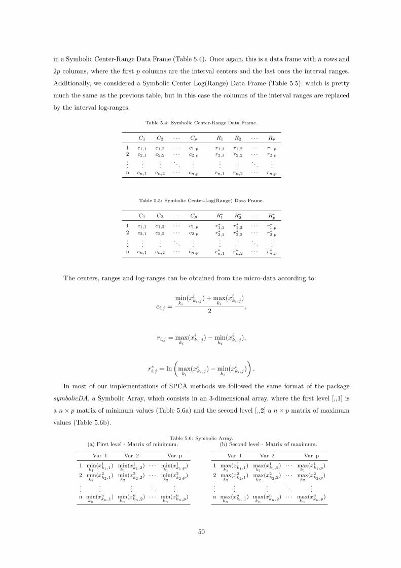
in a Symbolic Center-Range Data Frame (Table 5.4). Once again, this is a data frame with n rows and
2p columns, where the first p columns are the interval centers and the last ones the interval ranges.
Additionally, we considered a Symbolic Center-Log(Range) Data Frame (Table 5.5), which is pretty
much the same as the previous table, but in this case the columns of the interval ranges are replaced
by the interval log-ranges.
Table 5.4: Symbolic Center-Range Data Frame.
C1 C2 · · · Cp R1 R2 · · · Rp
1 c1,1 c1,2 · · · c1,p r1,1 r1,2 · · · r1,p2 c2,1 c2,2 · · · c2,p r2,1 r2,2 · · · r2,p...
......
. . ....
......
. . ....
n cn,1 cn,2 · · · cn,p rn,1 rn,2 · · · rn,p
Table 5.5: Symbolic Center-Log(Range) Data Frame.
C1 C2 · · · Cp R∗1 R∗
2 · · · R∗p
1 c1,1 c1,2 · · · c1,p r∗1,1 r∗1,2 · · · r∗1,p2 c2,1 c2,2 · · · c2,p r∗2,1 r∗2,2 · · · r∗2,p...
......
. . ....
......
. . ....
n cn,1 cn,2 · · · cn,p r∗n,1 r∗n,2 · · · r∗n,p
The centers, ranges and log-ranges can be obtained from the micro-data according to:
ci,j =minki
(xiki,j) + max
ki
(xiki,j)
2,
ri,j = maxki
(xiki,j)−minki
(xiki,j),
r∗i,j = ln
(maxki
(xiki,j)−minki
(xiki,j)
).
In most of our implementations of SPCA methods we followed the same format of the package
symbolicDA, a Symbolic Array, which consists in an 3-dimensional array, where the first level [,,1] is
a n× p matrix of minimum values (Table 5.6a) and the second level [,,2] a n× p matrix of maximum
values (Table 5.6b).
Table 5.6: Symbolic Array.
(a) First level - Matrix of minimum.
Var 1 Var 2 Var p
1 mink1
(x1k1,1) min
k1
(x1k1,2) · · · min
k1
(x1k1,p)
2 mink2
(x2k2,1) min
k2
(x2k2,2) · · · min
k2
(x2k2,p)
......
.... . .
...n min
kn
(xnkn,1) minkn
(xnkn,2) · · · minkn
(xnkn,p)
(b) Second level - Matrix of maximum.
Var 1 Var 2 Var p
1 maxk1
(x1k1,1) max
k1
(x1k1,2) · · · max
k1
(x1k1,p)
2 maxk2
(x2k2,1) max
k2
(x2k2,2) · · · max
k2
(x2k2,p)
......
.... . .
...n max
kn
(xnkn,1) maxkn
(xnkn,2) · · · maxkn
(xnkn,p)
50

In Table 5.7 we present a list of functions we developed to make conversions between the input
formats previously introduced. Moreover, all relationships listed are summarized in the diagram of
Figure 5.1.
Table 5.7: Conversion functions proposed.
Function Description From Table To Table
classic2symbArray Classic Data to Symbolic Array (2.3) (5.6)ClogR2symbArray Symbolic Center-Log(Range) to Symbolic Array (5.5) (5.6)ClogR2symbDF Symbolic Center-Log(Range) to Symbolic Min-Max (5.5) (5.2)CR2symbArray Symbolic Center-Range to Symbolic Array (5.4) (5.6)CR2symbDF Symbolic Center-Range to Symbolic Min-Max (5.4) (5.2)symbArray2ClogR Symbolic Array to Symbolic Center-Log(Range) (5.6) (5.5)symbArray2CR Symbolic Array to Symbolic Center-Range (5.6) (5.4)symbArray2symbDF Symbolic Array to Symbolic Min-Max (5.6) (5.2)symbArray2symbTab Symbolic Array to Symbolic Data Table (5.6) (5.3)symbDF2ClogR Symbolic Min-Max to Symbolic Center-Log(Range) (5.2) (5.5)symbDF2CR Symbolic Min-Max to Symbolic Center-Range (5.2) (5.4)symbDF2symbArray Symbolic Min-Max to Symbolic Array (5.2) (5.6)symbDF2symbTab Symbolic Min-Max to Symbolic Data Table (5.2) (5.3)symbTab2symbArray Symbolic Data Table to Symbolic Array (5.3) (5.6)symbTab2symbDF Symbolic Data Table to Symbolic Min-Max (5.3) (5.2)
5.2 Estimation methods and objects visualization
The interval-valued SPC methods under study (vide Table 3.1) have been implemented, with the
exception of Midpoints and radii PCA [45] and IPCA [27]. In the first we had problems with imple-
mentation of the rotation operator and in the second case difficulties associated with the determina-
tion of the interval-valued eigenvalues and eigenvectors. These methods, its main references, and the
function name are summarized in Table 5.8. Details for these functions are made available, in the
supplementary material to this thesis in a document similar to a Reference Manual.
Table 5.8: Names of the functions implementing SPCA methods: classical and robust estimators.
MethodFunction name
Classical Robust
CPCA [10] CPCA CPCAcovMcd A
CPCAgrid 1
VPCA [10] VPCA VPCAcovMcd A
VPCAcovMcd B
VPCAcovMcd C
VPCAcovMcd C2
VPCAgrid 1
CIPCA [59] CIPCA CIPCAcovMcd B
CIPCAcovMcd C
CIPCAcovMcd C2
Symbolic Covariance PCA [38] SymCovPCA SymCovPCAcovMcd B
SymCovPCAcovMcd C
SOPCA [36] SOPCA
General Formulation SimpleFormPCA
We have also included a function, SimpleFormPCA, where the CPCA, VPCA, CIPCA and SymCov-
PCA are implemented according to the general formulation, discussed in Chapter 3, which as stated
1 Using MAD or Qn estimator.
51

Fig
ure
5.1
:A
vaila
ble
pack
ages
for
SD
A(b
lue)
an
dco
nversio
nfu
nctio
ns
pro
posed
(red
).F
un
ction
nam
esin
bla
ckco
rrespon
dto
conversio
nfu
nctio
ns
availa
ble
in.
52

before, is more efficient and requires less computation time, being more suitable for high dimensional
datasets. In Table 5.8 are also listed the functions leading to the robust SPC proposed in this thesis.
For all these functions we have to define at least three arguments:
• data - An interval 3-dimensional array, in the format specified in Table 5.6.
• npc - Number of principal components to be retained.
• Cor - A logical value indicating whether the calculation should use the correlation matrix or the
covariance matrix.
Regarding the visualization, we have implemented routines to represent:
• Symbolic Objects in 2D (rectangles) and 3D (parallelepipeds);
• Scores of the SPCs in 2D and 3D (based on the MCARs).
For these graphical functions we need to provide: a matrix of minimum values, a matrix of maxi-
mum values, a vector of the colour identifiers to use, and the order in which the observations must be
represented. This last feature allows the user to try different orders, this is particular useful because
in the observations are plotted in a sequential way, so the last observations may overlap or even
cover the previous ones.
5.3 A Shiny web application to analyse Telecommunicationsdata
To make these new statistical techniques easily used in the analysis of real problems, we also developed
a web application, using the Shiny web application framework for , which includes several tools to
analyse, represent and perform PCA for conventional and interval data, in an interactive manner. For
interval data, it is possible to compare the traditional SPCA methods with all the new approaches
discussed in this work. The web application is available at http://52.16.30.111/shinyapp-marga/
and in this section we illustrate its potentialities with a Telecommunications dataset.
The fast development of the Internet over the last years has facilitated many tasks and brings us
endless resources, but at the same time makes us susceptible to dangerous threats to our safety and
well-being [46]. In fact, Internet attacks are a constant menace to Internet security, so it is essential
to find an effective way to characterize Internet traffic and define ways to distinguish attacks from
regular traffic. However, this is not an easy task because the continued development of computer
networks is accompanied by the appearance of a wide range of potential attacks that succeed to trick
and explore the weaknesses of the security systems.
In this work, we address a Telecommunications dataset introduced by [48] and already analysed
from a conventional point of view. This dataset was obtained in order to respect the actual functioning
of the Internet traffic and at the same time to have a reliable ground truth.
In particular, the observations were arranged into two classes of traffic (regular or licit and attacks
or illicit) and the application that generated each object is also known.
53

Regular or licit traffic:
• HTTP (web browsing),
• Torrent (file sharing),
• Streaming (video streaming),
• Video.
Attacks or illicit traffic:
• NMAP,
• Snapshots.
The regular traffic was generated by using the predominant Internet applications and was measured
in a controlled and protected environment to prevent the intrusion from outside threats, while the
attacks were internally emulated (vide [46, 48] for more details).
Similar to [46, 48], these data are composed by 917 observations (datastreams). Moreover, each
datastream aggregates all packets observed in a 5 minutes interval for which were obtained five traffic
characteristics in 0.1 seconds intervals (micro-data):
• Packets Up - number of upstream packets,
• Packets Down - number of downstream packets,
• Bytes Up - number of upstream bytes,
• Bytes Down - number of downstream bytes,
• Sessions - number of active TCP sessions.
The conventional approach to analyse this data passes through calculation of 8 summary statistics
for each of the 5 previous characteristics, namely: minimum (min), 1st quartile (Q1), median (med),
mean (m), 3rd quartile (Q3), maximum (max), standard deviation (sd) and median absolute deviation
(MAD). This gives a total of 40 variables for each observation, so we followed the suggestions developed
in [46] to remove some redundant variables from the analysis.
This dataset is in its nature symbolic, thus we can analyse it from this point of view. To do
that, we can naturally perform a temporal aggregation of the micro-data to obtain 917 observations
characterized by 5 interval-valued variables (macro-data).
In Figure 5.2a we graphically represent 2 of these 40 conventional variables and in Figure 5.2b we
represent the two correspondent interval-valued variables. The first thing that stands out is that in
2D, conventional data are represented by points and symbolic data are represented by rectangles.
54

0 10 20 30 40
050
100
150
Mean_Packets_Down
Mean
_Ses
soes
Type of application
HTTP (1)Torrent (2)Streaming (3)NMAP (4)Snapshot (5)Video (6)
●●●●●
●●●●●●●
●●●●●●
●
●●●●●
●●●●●●●●●●●●●
●●●●●●●
●●●
●
●●
●●●
●●
●
●●
●●●●
●
●●
●●
●
●
●
●
●
●
●
●●
●
●
●
●
●
●
●
●
●●
●
●
●
●
●
●●
●
●
●
●
●
●
●
●
●●
●●
●
●
●
●
●●
●
●
●
●
●
●
●
●
●
●
●
●
●
●
●
●
●
●●
●
●
●
●
●
●●
●
●●
●●
●
●
●
●
●
●
●●
●●
●●
●●
●
●
●
●
●
●
●●
●
●
●
●●
●
●●
●
● ●
●
●
●
●
●●
●
●
●
●
●
●●●
●
●
●
●
●
●
●
●
●●●●
●●●●
●
●
●
●●
●
●
●
●
●
●●
●●
●
●
●
●●●
●
●
●●
●
●●●●●
●
●●●
●
●●●●●
●
●
●
●●●●●
●
●
●
●
●●
●
●
●●●
●●
●●●●
●
●● ●
●
●
●
●
●
●
●
●
●●
●
●●
●●
●
●
●
●
●●●●●
●
●●
●
●●
●
●●●
●
●
●
●●●●●
●
●
●●●●●●●
●
●
●●●
●
●
●●
●●●●●
●●●●●●●●●●
●●●
●
●
●
●●
●
●
●●
●
●
●
●●●
●
●●
●
●●●
● ●
●
●
●
●
●
●●●●
●●
●●
●
●
●
●
●●
● ● ●●
●
●
●●
●●
●
●
●●●●
●
●
●
●●●●
●
●
●
●
●
●●
●
●
●
●
●
●
●
●
●
●
●
●● ●●●
●
●
●
●●
●●●●●●
●●●●●●●
●
●●●●●●●●●●●●●●●●●
●●●●●●●●●●●●
●●●●●●
●●●●●●●●●●●
●●●●●●
●●●
●●●●●●●●●
●●●●●●●●●●●●●●●●
●●●●●●●●●●●●●●●●●●●●●●●●●●●●●●●●●●●●●●●●●●●●●●●●●●●●●●●●●●●●●●●●●●●●●●●●●●●●●●●●●●●●●●●●●●●●●●●●●●●●●●●●●●●●●●●●●●●●●●●●●●●●●●●●●●●●●●●●●●●●●●●●●●●●●●●●●●●●●●●●●●●●●●●●●● ●●●●●●●●●●●●●●●●●●●●●●●●●●●●●●●●●●●●●●●●●●●●●●●●● ●●●●●●●●●●●●●●●●●●●●●●●●●●● ●●●●●●●●●●●●●●●●●●●●●●●●●●●●●●●●●●●●●●●●●●●●●●●●●●●●●●●●●●●●●●●●●●●●●●●●●●●●●●●●● ●●●●● ●●●●●●●●●●●●●●●●●●●●●●●●●●●●●●●●●●●●●●●●●●●●●
(a) Conventional data.
0 200 400 600 800
050
100
150
200
Packets_Down
Sess
oes
Type of application
HTTP (1)Torrent (2)Streaming (3)NMAP (4)Snapshot (5)Video (6)
(b) Interval-valued data.
Figure 5.2: Comparison between the two approaches - example.
The objective of our analyses is to demonstrate the potential of the symbolic approach as a new
and complementary perspective to visualize and model real data. In particular, we are interested in:
1. analyse the advantages of each approach and associated estimation methods;
2. compare the interpretations and the practical benefits of each approach;
3. identify the best methodology to analyse the problem of Internet traffic’s characterization;
4. identify the most relevant variables to characterize anomalous traffic.
Our objective is to use the dataset to illustrate and compare conventional and symbolic approaches.
We do not intend to give a full answer to the real problem, since it would demand methods to detect
symbolic outliers.
In fact, from a statistical perspective, traffic anomalies can be considered outliers, so we were trying
to define a procedure to detect outliers in interval-valued datasets. But despite all our experiments
and commitment we did not manage to conclude that task (for more details about this topic see our
proposals of future work on Chapter 6).
Moreover, methods based on Mahalanobis distance are being developed by Filzmoser et al. [25].
It will be interesting to compare both approaches to solve the anomaly detection problem in hand.
For this dataset in particular the main difficulties in detecting the outliers (anomalies) are the
small number of anomalies and their small variability. In fact, many of the anomalous observations
are equal.
In the following subsections we present the options available in our Shiny application and use this
dataset to conduct some experiments in the conventional and in the symbolic case to illustrate the
methodologies and visualization potentialities available.
55

5.3.1 Conventional Analysis
To open the Conventional Analysis panel of our Shiny web application, a user should:
1. access http://52.16.30.111/shinyapp-marga/
2. go to Internet Traffic Dataset Conventional approach
In the left panel (vide Figure 5.3) you can see the options available:
• type of variables transformation (none or logarithm);
• standardize or not;
• select the variables we want to use from the 40 available;
• method of PCs (Classical PCA, PCA robust Cov [56], PCAGRID [14], PCACR [13], ROBPCA
[32], and Spherical PCA [40] - for more details see Chapter 4);
• number of PCs to consider (1 up to the number of variables selected).
If you change one of these parameters, you will see how it affects the results in real time and
in each step of the analysis. This interface is extremely useful if, for instance, we are interested in
observing the impact of including a certain variable or group of variables in our analysis or not, which
is important when we have so many variables available.
Figure 5.3: Options available in the left panel - conventional approach.
56

In the right panel we have several tabs:
1. Descriptive statistics - we are able to compute some statistics for all the data or for a specific
class of observations. In this case, we organize the observations accordingly to the application
that generated it.
2. Representation of pairs of variables chosen between the selected ones;
In Figure 5.4 we have an example of a plot, in this particular image we can see that the anomalies
are few when compared with other classes and many of those are equal when described by these
two variables (Mean-bytes-Down and Mean-bytes-Up). It is difficult to spot NMAP in the plots
and Snapshot often appears divided into 2 groups.
For this representation we can choose which variables to plot in each axis, colour the observations
according to the class variable we want to consider (anomaly/licit or Internet application) and
define the order in which the observations are represented (box in blue). We also add a button
that allows the user to download the current plot in a .pdf format.
In the following tabs we have included some results for the obtained PCs.
3. Eigenvalues and the proportion of variability explained to help in choosing the number of
components to retain;
4. Loadings to make the interpretation of the principal components retained and define them;
5. Representation of Scores of pairs of PCs (the same options as for the representation of data)
6. Outliers detection based on the PCs (diagnostic chart - scores distance vs. orthogonal dis-
tance, where we can adjust the α, the probability of a regular observation being wrongly assigned
as an outlier. See [46] for further details).
Figure 5.4: Example of a scatterplot - conventional approach.
57

5.3.2 Symbolic Analysis
To open the Symbolic Analysis panel of our Shiny web application, a user should:
1. access http://52.16.30.111/shinyapp-marga/
2. go to Internet Traffic Dataset symbolic approach
In the left panel (Figure 5.5), once again you can see the options we have available:
• type of transformation of variables (none or logarithm);
• standardize or not;
• percentiles of trimmed anomalies and regular observations;
Since the definition of symbolic outliers is not clear, one of the techniques used was trimming the
data separately for anomalies and regular observations. This process is done separately because
the anomalies are few, have small variability and would be completely eliminated from the data
even for small global percentiles. The user must choose a percentile, q, between 0 and 20 for
each class of traffic. Then, for each object the minimum is replaced by the percentile q and the
maximum by the percentile 100− q.
• number of degenerate variables allowed;
A degenerate variable is a variable for which the minimum and the maximum are equal thus, the
interval is trivial and it is the same as considering a conventional variable. Since most methods
are not prepared to deal with degenerate variables, we may consider removing observations that
have too many of those variables. In fact, this parameter defines the number of degenerate
variables (from 0 to 5) we are willing to allow in each observation. If we set the parameter to 3,
all the observations with 4 or 5 degenerate variables are removed from the data.
• method of PCs (SPCA methods presented in Section 5.2);
• if the PCs must be obtained from the entire dataset or not.
As mentioned before, we have been trying to obtain a procedure to detect outliers in interval-
valued datasets. During this process, we had the need to separate the dataset in train and
test sets to properly evaluate the performance of our procedures. Thus, we implemented the
possibility of calculating the SPCs based on the test set or on the entire dataset.
58

Figure 5.5: Options available in the left panel - symbolic approach.
Like in the conventional approach, in the right panel we have several tabs:
1. Descriptive statistics - symbolic mean, standard deviation and variance to summarize the
data;
2. Degenerate variables
In this tab, there are two tables. The first table allow finding out how many observations of
a given type of traffic have a specific degenerate variable. For example, with this table we
can determine about how many observations generated by Video have the variable Packets Up
degenerate. In the second table we have the observations distributed according to the number
of degenerate variables they have and the type of traffic / application they belong. For instance,
we can find out how many anomalous observations have 3 degenerate variables or how many
observations generated by Torrent have 5 degenerate variables.
3. SOs’ representation in 2D (the options available are the same as for the conventional ap-
proach);
In Figure 5.6 we have represented Sessions vs. Sessions and we can distinguish different groups of
observations generated by Torrent. The observations with lower numbers of sessions correspond
to less popular torrent files (maybe classics, rare to find or even less available files) and the
observations with higher numbers of active sessions are related with popular and recent files.
59

Figure 5.6: Example of a plot representing two symbolic variables - symbolic approach.
In the following tabs we have included some results for the SPCs obtained for interval-valued
data.
4. Eigenvalues and the proportion of associated eigenvalues;
5. Loadings, weights that define the SPC;
6. Scores Plot - representation of symbolic scores of SPCs obtained according to MCAR method.
7. Detection of outliers and performance measures - Diagnostic chart, scores distance vs.
orthogonal distance. Eventhough, this tab is left in the Shiny application these features need
further study and are not discussed in this thesis. Some comments on this topic are presented
in Chapter 6.
We noticed that the representations of the scores associated with several classical SPCA methods
are quite similar thus, it is really hard to choose the most appropriate method. In fact, the classical
SPCA methods and most of the approaches based on robust covariance matrices led to similar results.
As an example, in Figure 5.7a we have the scores representation of the first two principal components
obtained with the method CPCA. The results represented in Figure 5.7b were obtained for the method
VPCAgridQN. This method and all the other robust SPCA methods based on PP were the only ones
to present more discordant patterns.
60
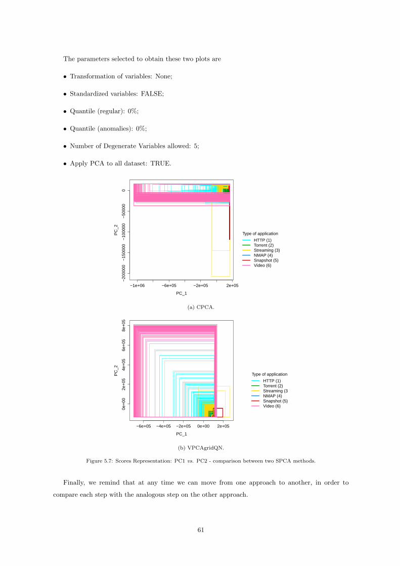
The parameters selected to obtain these two plots are
• Transformation of variables: None;
• Standardized variables: FALSE;
• Quantile (regular): 0%;
• Quantile (anomalies): 0%;
• Number of Degenerate Variables allowed: 5;
• Apply PCA to all dataset: TRUE.
−1e+06 −6e+05 −2e+05 2e+05
−20
0000
−15
0000
−10
0000
−50
000
0
PC_1
PC
_2
Type of application
HTTP (1)Torrent (2)Streaming (3)NMAP (4)Snapshot (5)Video (6)
(a) CPCA.
−6e+05 −4e+05 −2e+05 0e+00 2e+05
0e+
002e
+05
4e+
056e
+05
8e+
05
PC_1
PC
_2
Type of application
HTTP (1)Torrent (2)Streaming (3)NMAP (4)Snapshot (5)Video (6)
(b) VPCAgridQN.
Figure 5.7: Scores Representation: PC1 vs. PC2 - comparison between two SPCA methods.
Finally, we remind that at any time we can move from one approach to another, in order to
compare each step with the analogous step on the other approach.
61

Chapter 6
Conclusions
6.1 General overview
One of the objectives of this thesis is to develop a population formulation of SPCA. To accomplish this
task we study and propose population formulations for the symbolic covariance matrix associated with
a multivariate interval-valued random vector. These formulations are based on the several proposals
for symbolic variance and covariance available in the literature, for this type of symbolic vectors.
We conclude that centers and ranges have different importance in the construction of these matrices.
In fact, all definitions take into consideration the covariance matrix of the centers, but they differ
in the role played by the ranges variability. The findings about the several symbolic covariance
matrices lead us to a better understanding of the SPC methods available in the literature. In this
thesis, we give special attention to the first two proposals (CPCA and VPCA) and two of the most
recent methods (CIPCA and SymCovPCA). We proved that each method uses a different definition
of symbolic covariance matrix to obtain the weights defining the SPC. Furthermore, we proposed a
general methodology to compute the methods based on the theoretical formulations deduced. This
general procedure allow obtaining simplifications, additional insight and unification of the algorithms
of the methods, as well as it facilitates the establishment of properties of the SPC.
The next step in a SPC method based on a symbolic-conventional-symbolic strategy is to represent
the object back into a symbolic framework. The simplest and most used method is based on MCAR
representation. As before, we have derived an explicit and straightforward formula that leads to
the definition of a SPC score in an interval-valued form. In a similar way to what happens in the
conventional framework, the interval defining the kth SPC has a center that is the linear combination
of the centers of the original symbolic variables, whose weights are determined by the kth eigenvector
of a given symbolic covariance matrix, which depends on the estimation method under study. The
ranges are also a linear combination of the original ranges, but to insure that all the ranges are positive,
the method considers the same weights as before, but using their absolute value.
Regarding the robust PC estimation methods for interval-valued data, it should be noted that,
before we developed these theoretical formulations, our approaches only included robust versions of
CPCA and VPCA, namely the PP approach and the approach A based on the robust covariance
62

estimates. So, considering the general population formulations, proposed in a previous chapter, al-
lows defining approaches B, C and C2 (vide Section 4.2.1 for details), that can also be applied to
obtain robust estimators based on CIPCA and SymCovPCA. More efficient robust versions for VPCA
were also obtained since the new approaches do not require the computation of the vertices matrix.
Moreover, the simulation study conducted allowed concluding that, as we expected, these methods
can accommodate atypical observations. We can also conclude that the methods based on the robust
covariance estimates proved to be more efficient than the ones based on PP. This is not coeherent
with what happens in conventional PCA and requires further investigation.
To make this new statistical tools easily used in the analysis of real problems, besides of implement-
ing these routines in the statistical software , we also developed a web application, using the Shiny
web application framework for . This application includes several tools to analyse, represent, and
perform (classical and robust) SPCA on interval-valued data, in an interactive manner and provides
an easier way to analyse and explore data.
Moreover, we also implemented routines to make conversions between the different representations
of interval-valued data used in several packages for SDA. Our objective was to simplify the process
of using functions from different packages consecutively, in the same analysis. Until now this was
a difficult task since these packages were developed independently and each one requires input and
output data in a specific format.
Finally, we believe that the line of work followed in this thesis can contribute to turn SPCA into
a more attractive and additional versatile tool to analyse real data.
6.2 Future work
The main goals of this thesis were achieved, however during our research we come up with a few ideas
and questions that we would like to have had the opportunity to investigate further. In what follows,
we point out several aspects we consider worthwhile investigating in future work.
In Chapter 2 we discussed what a symbolic covariance matrix is, according to the proposals avail-
able in the literature. Nevertheless, other properties of these matrices could have been explored, if we
had the time, which we plan to do in a near future.
Similarly, the other properties associated with SPC have not been proposed due to the same reason,
and are left for future analysis.
Regarding the robust PC estimation methods, the experiments performed considering contamina-
tions in the log-ranges lead to unsatisfactory results. We suspect that the contamination done in the
log-range has an exponential impact in the ranges mean, and variance, which may be the source of
the problems encountered.
As mentioned in Chapter 5, we have performed several experiments in an attempt to define a
outlier detection procedure based on the results of the PCs for interval-valued data. Similarly to
the conventional approach, we were trying to compute a symbolic version of the Mahalanobis and
orthogonal distance based on SPCs scores, in order to represent the observations in a diagnostic
63

plot. The population formulation of the SPCs allowed computing the Mahalanobis distance, however
defining the cut-of value has proved to be a more complicated task. In fact, we have considered several
alternatives to compute this value but we did not include these results in this thesis since they need
further investigation.
Another topic we would also like to investigate further is the effect of degenerate variables in the
population formulations we have developed for the covariance matrices and SPC methods. According
to our intuition and based on some calculations we think that to accommodate degenerate variables
we would have to incorporate a term referring to the proportion of the total vertices associated to
degenerate observations. Initial results were obtained but a lot of work has to be done around this
issue.
64

References
[1] P. Bertrand and F. Goupil. Descriptive statistics for symbolic data. In H.-H. Bock and E. Diday,
editors, Analysis of Symbolic Data, Studies in Classification, Data Analysis, and Knowledge
Organization, pages 106–124. Springer Berlin Heidelberg, 2000. 12
[2] L. Billard. Sample Covariance Functions for Complex Quantitative Data. In Proceedings of World
IASC Conference, Yokohama, Japan,, pages 157–163, 2008. 13, 14, 28
[3] L. Billard and E. Diday. From the statistics of data to the statistics of knowledge: Symbolic data
analysis. Journal of the American Statistical Association, 98:470–487, 2003. 13
[4] L. Billard and E. Diday. Symbolic Data Analysis: Conceptual Statistics and Data Mining. John
Wiley & Sons, 2006. ix, 7, 13, 14
[5] H. H. Bock and E. Diday. Analysis of Symbolic Data: Exploratory Methods for Extracting Sta-
tistical Information from Complex Data. Springer-Verlag New York, Inc., 2000. 6
[6] G. Box. Non-normality and tests on variance. Biometrika, 40:318–335, 1953. 35
[7] B. Brahim and S. Makosso-Kallyth. GPCSIV: Generalized Principal Component of Symbolic In-
terval variables, 2013. URL http://CRAN.R-project.org/package=GPCSIV. R package version
0.1.0. 48
[8] B. Brahim and S. Makosso-Kallyth. GraphPCA: GraphPCA, Graphical tools of histogram PCA,
2014. URL http://CRAN.R-project.org/package=GraphPCA. R package version 1.0. 48
[9] P. Brito and A. Duarte Silva. Modelling interval data with normal and skew-normal distributions.
Journal of Applied Statistics, 39(1):3–20, 2012. xi, 9, 10, 11, 43
[10] P. Cazes, A. Chouakria, E. Diday, and Y. Schektman. Extension de l’analyse en composantes
principales a des donnees de type intervalle. Revue de Statistique Appliquee, 45(3):5–24, 1997. 2,
17, 18, 19, 20, 30, 51
[11] A. Chouakria. Extension des Methodes d’Analyse Factorielle a des Donnees de Type Intervalle.
PhD thesis, Universite Paris-Dauphine, 1998. 30
[12] C. Croux and A. Ruiz-Gazen. A Fast Algorithm for Robust Principal Components Based on
Projection Pursuit. In 12th International Conference on Computational Statistics – COMPSTAT
1996, Barcelona, Spain, pages 211–216, 1996. 42
65

[13] C. Croux and A. Ruiz-Gazen. High breakdown estimators for principal components: the
projection-pursuit approach revisited. Jornal of Multivariate Analysis, 95(1):206–226, 2005. 42,
56
[14] C. Croux, P. Filzmoser, and M. R. Oliveira. Algorithms for Projection - Pursuit robust principal
component analysis. Chemometrics and Intelligent Laboratory Systems, 87(2):218–225, 2007. 42,
56
[15] E. de A. Lima Neto, G. M. Cordeiro, and F. de A.T. de Carvalho. Bivariate symbolic regression
models for interval-valued variables. Journal of Statistical Computation and Simulation, 81(11):
1727–1744, 2011. 9
[16] F. d. A. De Carvalho, P. Brito, and H.-H. Bock. Dynamic clustering for interval data based on
l2 distance. Computational Statistics, 21(2):231–250, 2006. 12
[17] E. Diday. The symbolic approach in clustering and related methods of Data Analysis. In Pro-
ceedings of First conference IFCS,Aachen, Germany. H. Bock ed.North-Holland, 1987. 1
[18] E. Diday and M. Noirhomme-Fraiture. Symbolic Data Analysis and the SODAS Software. Wiley-
Interscience, New York, NY, USA, 2008. 25, 48
[19] M. A. Domingues. Metodos robustos em regressao linear para dados simbolicos do tipo intervalo.
PhD thesis, Universidade Federal de Pernambuco, Recife, 2010. 36
[20] M. A. Domingues, R. De Souza, and F. Cysneiros. A robust method for linear regression of
symbolic interval data. Pattern Recognition Letters, 31(13):1991 – 1996, 2010. 36
[21] D. Donoho and P. Huber. The notion of breakdown point. A Festschrift for Erich Lehmann,
page 157–184, 1983. 38
[22] A. Douzal-Chouakria, L. Billard, and E. Diday. Principal Component Analysis for Interval-Valued
Observations. Statistical Analysis and Data Mining, (4):229–246, 2011. 23, 32
[23] A. Dudek, M. Pelka, and J. Wilk. symbolicDA: Analysis of symbolic data, 2013. URL http:
//CRAN.R-project.org/package=symbolicDA. R package version 0.4-1. 48
[24] R. Q. Filho and R. Fagundes. ISDA.R: Interval symbolic data analysis for R, 2012. URL http:
//CRAN.R-project.org/package=ISDA.R. R package version 1.0. 48, 49
[25] P. Filzmoser, P. Brito, and A. Duarte Silva. Outlier Detection in Interval Data. In 21st Interna-
tional Conference on Computational Statistics – COMPSTAT 2014, Geneva, Switzerland, 2014.
xi, 11, 36, 41, 55
[26] J. Friedman and J. Tukey. A projection pursuit algorithm for exploratory data analysis. IEEE
Transactions on Computers, (C-23):881–890, 1974. 41
66

[27] F. Gioia and C. N. Lauro. Principal Component Analysis on Interval Data. Computational
Statistics, 21(2):343–363, 2006. 17, 25, 30, 51
[28] A. S. Hadi and A. Luceno. Maximum trimmed likelihood estimators: a unified approach, exam-
ples, and algorithms. Computational Statistics & Data Analysis, 25(3):251 – 272, 1997. 41
[29] P. Huber. Robust estimation of a location parameter. The Annals of Mathematical Statistics, 35:
73–101, 1964. 35
[30] P. J. Huber. Projection pursuit. The Annals of Statistics, 13(2):435–475, 1985. 41
[31] M. Hubert, P. J. Rousseeuw, and S. Verboven. A fast method for robust principal components
with applications to chemometrics. Chemometrics and Intelligent Laboratory Systems, 60(1–2):
101 – 111, 2002. 42
[32] M. Hubert, P. Rousseeuw, and K. Vanden Branden. ROBPCA: A new approach to robust
principal component analysis. Technometrics, 47(1):64–79, 2005. 43, 56
[33] A. Irpino. HistDAWass: Histogram-Valued Data Analysis, 2015. URL http://CRAN.R-project.
org/package=HistDAWass. R package version 0.1.3. 48
[34] A. Irpino, C. Lauro, and R. Verde. Visualizing symbolic data by closed shapes. In Between Data
Science and Applied Data Analysis, Studies in Classification, Data Analysis, and Knowledge
Organization, pages 244–251. Springer Berlin Heidelberg, 2003. 34
[35] R. A. Johnson and D. W. Wichern. Applied Multivariate Statistical Analysis. Prentice-Hall, Inc.,
Upper Saddle River, NJ, USA, 2007. 16, 33
[36] C. N. Lauro and F. Palumbo. Principal component analysis of interval data: a symbolic data
analysis approach. Computational Statistics, 15(1):73–87, 2000. 17, 24, 30, 51
[37] J. Le-Rademacher. Principal Component Analysis for Interval-Valued and Histogram-Valued Data
and Likelihood Functions and Some Maximum Likelihood Estimators for Symbolic Data. PhD
thesis, University of Georgia, Athens, GA., 2008. 19, 28
[38] J. Le-Rademacher and L. Billard. Symbolic Covariance Principal Component Analysis and Visu-
alization for Interval-Valued Data. Computational and Graphical Statistics, 21(2):413–432, 2012.
ix, 2, 17, 18, 28, 30, 33, 34, 48, 51
[39] G. Li and Z. Chen. Projection-Pursuit Approach to Robust Dispersion Matrices and Principal
Components: Primary Theory and Monte Carlo. Journal of the American Statistical Association,
80(391):759–766, 1985. 42
[40] N. Locantore, J. Marron, D. Simpson, N. Tripoli, Zhang, J.T., and K. Cohen. Robust principal
component analysis for functional data. 43, 56
67

[41] R. Maronna. Principal Components and Orthogonal Regression Based on Robust Scales. Tech-
nometrics, 47:264–273, 2005. 43
[42] R. Moore. Interval Analysis. Prentice-Hall, Inc., Englewood Cliffs, NJ, 1966. 25
[43] E. L. Neto and C. Vasconcelos. iRegression: Regression methods for interval-valued variables,
2012. URL http://CRAN.R-project.org/package=iRegression. R package version 1.2. 48, 49
[44] N. Neykov, P. Filzmoser, R. Dimova, and P. Neytchev. Robust fitting of mixtures using the
trimmed likelihood estimator. Computational Statistics & Data Analysis, 52(1):299 – 308, 2007.
41
[45] F. Palumbo and C. N. Lauro. A PCA for interval-valued data based on midpoints and radii. New
developments in Psychometrics, pages 641–648, 2003. 17, 24, 30, 51
[46] C. Pascoal. Contributions to Variable Selection and Robust Anomaly Detection in Telecommuni-
cations. PhD thesis, Tecnico Lisboa, UL, Lisboa, 2014. 53, 54, 57
[47] C. Pascoal, M. Oliveira, A. Pacheco, and R. Valadas. Detection of outliers using robust principal
component analysis: A simulation study. In Combining Soft Computing and Statistical Methods
in Data Analysis, volume 77 of Advances in Intelligent and Soft Computing, pages 499–507. 2010.
42
[48] C. Pascoal, M. R. Oliveira, R. Valadas, P. Filzmoser, P. Salvador, and A. Pacheco. Robust feature
selection and robust PCA for internet traffic anomaly detection. In INFOCOM, 2012 Proceedings
IEEE, pages 1755–1763, 2012. 53, 54
[49] R Core Team. R: A Language and Environment for Statistical Computing. R Foundation for
Statistical Computing, Vienna, Austria, 2015. URL https://www.R-project.org/. 4, 48
[50] O. Rodriguez, O. Calderon, and R. Zuniga. RSDA: R to Symbolic Data Analysis, 2014. URL
http://CRAN.R-project.org/package=RSDA. R package version 1.2. 48
[51] P. Rousseeuw. Multivariate Estimation with High Breakdown Point. Mathematical Statistics and
Applications, B:283–297, 1985. 38
[52] P. Rousseeuw and K. Van Driessen. A Fast Algorithm for the Minimum Covariance Determinant
Estimator. Technometrics, 41:212–223, 1999. 38, 39
[53] P. Rousseeuw, C. Croux, V. Todorov, A. Ruckstuhl, M. Salibian-Barrera, T. Verbeke, M. Kolle,
and M. Maechler. robustbase: Basic Robust Statistics, 2014. URL http://CRAN.R-project.
org/package=robustbase. R package version 0.92-2. 39
[54] P. D. Silva and P. Brito. MAINT.Data: Model and Analyse Interval Data, 2011. URL http:
//CRAN.R-project.org/package=MAINT.Data. R package version 0.2. 48
68
[55] Y. Terada and P. J. F. Groenen. smds: Symbolic Multidimensional Scaling, 2015. URL http:
//CRAN.R-project.org/package=smds. R package version 1.0. 48
[56] V. Todorov and P. Filzmoser. An object-oriented framework for robust multivariate analysis.
Journal of Statistical Software, 32(3):1–47, 2009. URL http://www.jstatsoft.org/v32/i03/.
56
[57] O. Toomet. intReg: Interval Regression, 2012. URL http://CRAN.R-project.org/package=
intReg. R package version 0.1-2. 48
[58] M. Vilela. Analise em componentes principais de dados intervalares. Technical report, Tecnico
Lisboa, UL, Lisboa, 2013. 5
[59] H. Wang, R. Guan, and J. Wu. CIPCA: Complete-Information-based Principal Component
Analysis for Interval-valued Data. Neurocomputing, 86:158–169, 2012. 2, 17, 18, 23, 26, 27, 30,
44, 51
69
