Wayne State University

Wayne State University Dissertations

1-1-2016

Principal Component Analysis-Based AnatomicalMotion Models For Use In Adaptive RadiationTherapy Of Head And Neck Cancer PatientsMikhail Aleksandrovich ChetvertkovWayne State University,

Follow this and additional works at: http://digitalcommons.wayne.edu/oa_dissertations

Part of the Mathematics Commons, Oncology Commons, and the Physics Commons

This Open Access Dissertation is brought to you for free and open access by DigitalCommons@WayneState. It has been accepted for inclusion inWayne State University Dissertations by an authorized administrator of DigitalCommons@WayneState.

Recommended CitationChetvertkov, Mikhail Aleksandrovich, "Principal Component Analysis-Based Anatomical Motion Models For Use In AdaptiveRadiation Therapy Of Head And Neck Cancer Patients" (2016). Wayne State University Dissertations. Paper 1522.

PRINCIPAL COMPONENT ANALYSIS-BASED ANATOMICAL MOTION MODELS FOR USE IN ADAPTIVE RADIATION THERAPY OF HEAD AND NECK CANCER

PATIENTS

by

MIKHAIL A. CHETVERTKOV

DISSERTATION

Submitted to the Graduate School

of Wayne State University,

Detroit, Michigan

in partial fulfillment of the requirements

for the degree of

DOCTOR OF PHILOSOPHY

2016

MAJOR: MEDICAL PHYSICS

Approved By:

Advisor Date

© COPYRIGHT BY

MIKHAIL A. CHETVERTKOV

2016

All Rights Reserved

ii

DEDICATION

To my mom, dad, sister, grandmother and grandfather and all my family in Russia whose support

and love I could always feel even from overseas.

To my uncle, aunt and cousins for their help and support during my life in Detroit.

Finally, to my wife, Zhenya, for her endless love and support.

iii

ACKNOWLEDGEMENTS

I would like to thank my dissertation committee: Dr. Indrin J. Chetty, Dr. Jay

Burmeister, Dr. Michael Snyder, Dr. Joseph Rakowski, Dr. Stephen Brown, and in

particular Dr. J. James Gordon for their help, support, constructive criticism and

suggestions throughout this process.

I would also like to thank the ART H&N group members: Dr. Jinkoo Kim, Dr. Chang

Liu, Dr. Akila Kumarasiri, Dr. Hualiang Zhong and Dr. Farzan Siddiqui for the many

insightful discussions and thoughts during our meetings.

Henry Ford Health System holds research agreements with Philips healthcare, and

this research was supported in part by a grant from Varian Medical Systems, Palo Alto,

CA.

iv

PREFACE

Note to the reader:

Chapter 1 defines the clinical problem and provides a brief introduction to

conventional methods of handling geometric uncertainties inherent in the delivery of

radiation for the treatment of cancer. Chapter 1 also presents the rationale of anatomical

motion model development for improved radiation therapy outcomes.

Chapters 2-4 of this dissertation include patient-specific motion models based on

standard and regularized Principal Component Analysis (PCA) approaches, and

dosimetric outcomes that follow radiation treatments based on these models.

Finally, Chapter 5 presents conclusions and discussion of future directions.

v

TABLE OF CONTENTS

Dedication _________________________________________________________ ii

Acknowledgments _____________________________________________________ iii

Preface _________________________________________________________ iv

List of Tables ________________________________________________________ viii

List of Figures _________________________________________________________ ix

List of Abbreviations ___________________________________________________ xii

Chapter 1 “Introduction” _________________________________________________ 1

Geometric Uncertainties in Radiation Therapy __________________________ 1

Conventional Method of Handling Geometric Uncertainties ________________ 3

Conventional Method of Handling OAR Uncertainties _______________ 4

Conventional Method of Handling Delineation Uncertainties __________ 6

Role of Image-Guided Radiation Therapy and Adaptive Radiation Therapy in Handling Uncertainties _____________________________________ 6

Motivation for Motion Model Development in Radiation Therapy for Head and Neck Patients ________________________________________________________ 7

Statement of the Problem __________________________________________ 7

Chapter 2 “Standard Principal Component Analysis Model of Anatomical Changes in Head and Neck Patients” ________________________________________________ 9

Introduction _____________________________________________________ 9

Materials and Methods ____________________________________________ 9

Clinical and Simulated Image Data ______________________________ 9

Deformation Vector Fields Data _______________________________ 12

Clinical Deformation Vector Fields _____________________________ 13

Synthetic Deformation Vector Fields ____________________________ 13

vi

PCA Models – Standard PCA _________________________________ 16

Predictive Model ___________________________________________ 17

Model Evaluation __________________________________________ 19

Results _______________________________________________________ 22

Qualitative Evaluation _______________________________________ 22

Quantitative Evaluation ______________________________________ 24

Discussion _____________________________________________________ 26

Qualitative Evaluation _______________________________________ 26

Quantitative Evaluation ______________________________________ 28

Conclusion _____________________________________________________ 30

Chapter 3 “Regularized Principal Component Analysis Model of Anatomical Changes in Head and Neck Patients” _______________________________________________ 31

Introduction ____________________________________________________ 31

Materials and Methods ___________________________________________ 31

PCA Models – Regularized PCA ______________________________ 31

Results _______________________________________________________ 32

Qualitative Evaluation _______________________________________ 32

Quantitative Evaluation ______________________________________ 35

Discussion _____________________________________________________ 44

Qualitative Evaluation _______________________________________ 44

Quantitative Evaluation ______________________________________ 45

PCA Performance __________________________________________ 46

Prior Applications of PCA ____________________________________ 50

Potential for Regularized PCA ________________________________ 51

vii

Study Limitations __________________________________________ 53

Conclusion _____________________________________________________ 55

Chapter 4 “Dosimetric Assessment of Effects of Systematic and Random Fraction-to-Fraction Anatomical Changes in Head and Neck Patients” _____________________ 56

Introduction ____________________________________________________ 56

Materials and Methods ___________________________________________ 57

Results _______________________________________________________ 61

Discussion _____________________________________________________ 70

Conclusion _____________________________________________________ 74

Chapter 5 “Conclusions and Future Work” __________________________________ 75

Summary of Findings _____________________________________________ 75

Future Work ____________________________________________________ 76

Appendix “Standard Principal Component Analysis Matrix Operations” ____________ 79

References ________________________________________________________ 82

Abstract ________________________________________________________ 91

Autobiographical Statement _____________________________________________ 94

viii

LIST OF TABLES

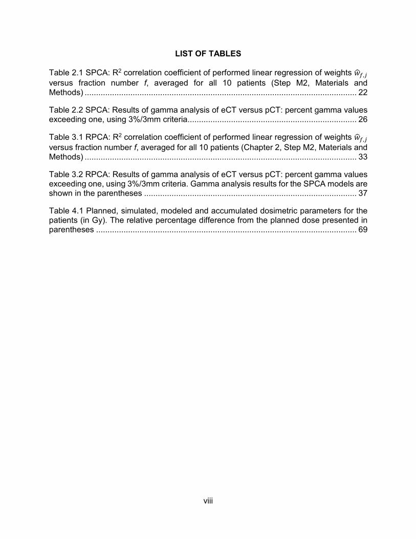
Table 2.1 SPCA: R2 correlation coefficient of performed linear regression of weights ���,�

versus fraction number f, averaged for all 10 patients (Step M2, Materials and Methods) ....................................................................................................................... 22

Table 2.2 SPCA: Results of gamma analysis of eCT versus pCT: percent gamma values exceeding one, using 3%/3mm criteria .......................................................................... 26

Table 3.1 RPCA: R2 correlation coefficient of performed linear regression of weights ���,�

versus fraction number f, averaged for all 10 patients (Chapter 2, Step M2, Materials and Methods) ....................................................................................................................... 33

Table 3.2 RPCA: Results of gamma analysis of eCT versus pCT: percent gamma values exceeding one, using 3%/3mm criteria. Gamma analysis results for the SPCA models are shown in the parentheses ............................................................................................. 37

Table 4.1 Planned, simulated, modeled and accumulated dosimetric parameters for the patients (in Gy). The relative percentage difference from the planned dose presented in parentheses .................................................................................................................. 69

ix

LIST OF FIGURES

Figure 2.1: Blended pCT and wCT images of four (out of ten) patients; A - parotid gland shrinkage, B - parotid gland shrinkage and weight loss, C - Tumor shrinkage in the oropharynx, D - lymph node shrinkage in the left .......................................................... 10

Figure 2.2: In-house developed interactive software tool (Matlab®) to perform warping of the images ..................................................................................................................... 11

Figure 2.3: Early, linear and late models of patient response ........................................ 15

Figure 2.4: Relationship between measured and predicted DVFs ................................ 19

Figure 2.5: SPCA: Results of SPCA models generated from synthetic DVFs for patient D, for whom PCA modeling gave the best results. ............................................................. 23

Figure 2.6: SPCA: Results of SPCA models generated from synthetic DVFs for patient A, for whom PCA modeling gave the worst results ............................................................ 24

Figure 2.7: SPCA: Mean lengths of the image error as a function of the number of fractions

F. Vector lengths are scaled by 1/√. Both the mean and standard deviation of the lengths of the image error vectors decrease as F increases ......................................... 25

Figure 3.1: RPCA: Results of RPCA models generated from synthetic DVFs for patient D, for whom PCA modeling gave the best results ......................................................... 34

Figure 3.2: RPCA: Results of RPCA models generated from synthetic DVFs for patient A, for whom PCA modeling gave the worst results ............................................................ 35

Figure 3.3: RPCA: Mean lengths of the image error as a function of the number of

fractions F. Vector lengths are scaled by 1/√. Both the mean and standard deviation of the lengths of the image error vectors decrease as F increases. SPCA results are represented by dashed grey lines ................................................................................. 36

Figure 3.4: Leading EDVF weight averaged for SPCA and RPCA models generated from synthetic DVFs for a patient who experienced parotid shrinkage. Results are shown for the PCA models generated from first 5 fractions (top), half of the fractions (middle) and all-but-last fraction (bottom). .......................................................................................... 38

Figure 3.5: RPCA: 1st and 2nd EDVF weights for RPCA models generated from synthetic DVFs for a patient who experienced parotid shrinkage. A linear response model was

assumed (Chapter 2, Materials and Methods), and κ = 5 in equation 2.1, ensuring that DVFs incorporated approximately 5 times the level of random motion seen in clinical CBCTs ........................................................................................................................... 39

Figure 3.6: RPCA: 1st, 2nd and 3rd EDVF weights for RPCA models generated from clinical DVFs for a patient who experienced weight loss in the left neck ................................... 41

x

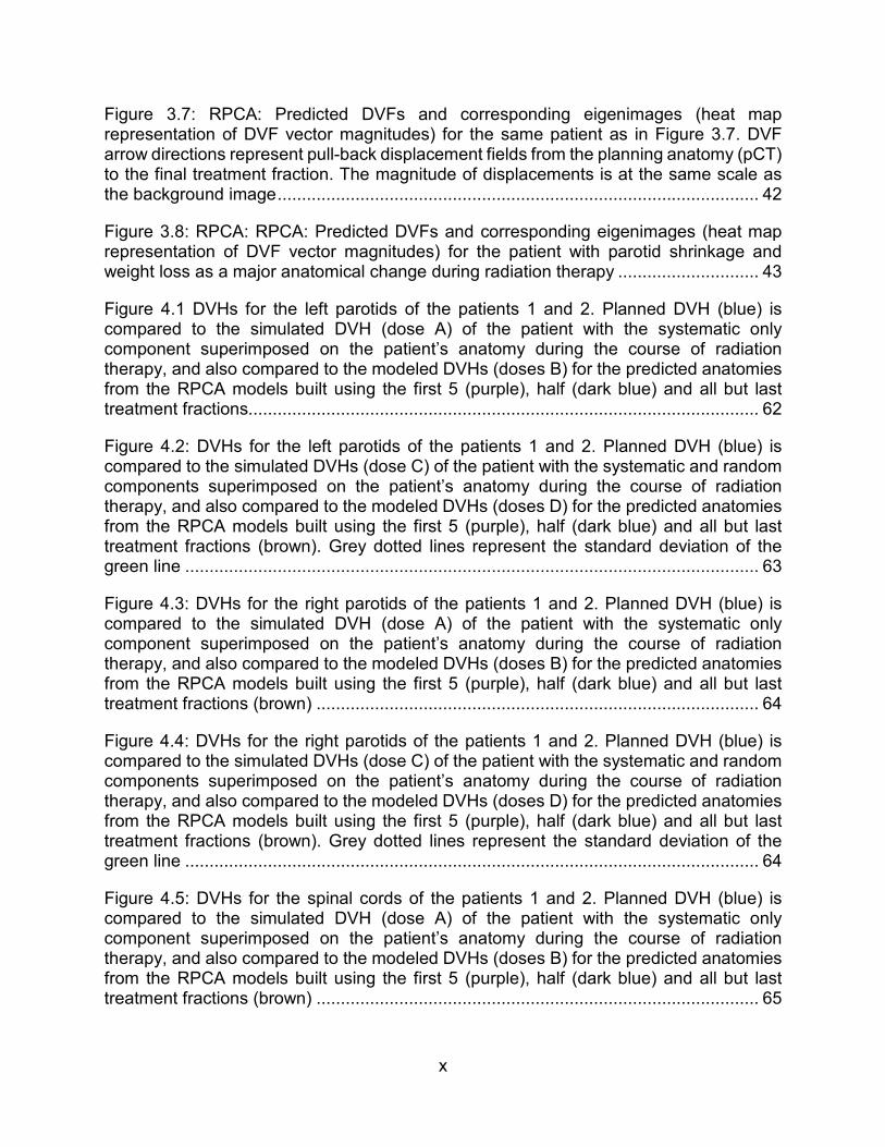
Figure 3.7: RPCA: Predicted DVFs and corresponding eigenimages (heat map representation of DVF vector magnitudes) for the same patient as in Figure 3.7. DVF arrow directions represent pull-back displacement fields from the planning anatomy (pCT) to the final treatment fraction. The magnitude of displacements is at the same scale as the background image ................................................................................................... 42

Figure 3.8: RPCA: RPCA: Predicted DVFs and corresponding eigenimages (heat map representation of DVF vector magnitudes) for the patient with parotid shrinkage and weight loss as a major anatomical change during radiation therapy ............................. 43

Figure 4.1 DVHs for the left parotids of the patients 1 and 2. Planned DVH (blue) is compared to the simulated DVH (dose A) of the patient with the systematic only component superimposed on the patient’s anatomy during the course of radiation therapy, and also compared to the modeled DVHs (doses B) for the predicted anatomies from the RPCA models built using the first 5 (purple), half (dark blue) and all but last treatment fractions......................................................................................................... 62

Figure 4.2: DVHs for the left parotids of the patients 1 and 2. Planned DVH (blue) is compared to the simulated DVHs (dose C) of the patient with the systematic and random components superimposed on the patient’s anatomy during the course of radiation therapy, and also compared to the modeled DVHs (doses D) for the predicted anatomies from the RPCA models built using the first 5 (purple), half (dark blue) and all but last treatment fractions (brown). Grey dotted lines represent the standard deviation of the green line ...................................................................................................................... 63

Figure 4.3: DVHs for the right parotids of the patients 1 and 2. Planned DVH (blue) is compared to the simulated DVH (dose A) of the patient with the systematic only component superimposed on the patient’s anatomy during the course of radiation therapy, and also compared to the modeled DVHs (doses B) for the predicted anatomies from the RPCA models built using the first 5 (purple), half (dark blue) and all but last treatment fractions (brown) ........................................................................................... 64

Figure 4.4: DVHs for the right parotids of the patients 1 and 2. Planned DVH (blue) is compared to the simulated DVHs (dose C) of the patient with the systematic and random components superimposed on the patient’s anatomy during the course of radiation therapy, and also compared to the modeled DVHs (doses D) for the predicted anatomies from the RPCA models built using the first 5 (purple), half (dark blue) and all but last treatment fractions (brown). Grey dotted lines represent the standard deviation of the green line ...................................................................................................................... 64

Figure 4.5: DVHs for the spinal cords of the patients 1 and 2. Planned DVH (blue) is compared to the simulated DVH (dose A) of the patient with the systematic only component superimposed on the patient’s anatomy during the course of radiation therapy, and also compared to the modeled DVHs (doses B) for the predicted anatomies from the RPCA models built using the first 5 (purple), half (dark blue) and all but last treatment fractions (brown) ........................................................................................... 65

xi

Figure 4.6: DVHs for the spinal cords of the patients 1 and 2. Planned DVH (blue) is compared to the simulated DVHs (dose C) of the patient with the systematic and random components superimposed on the patient’s anatomy during the course of radiation therapy, and also compared to the modeled DVHs (doses D) for the predicted anatomies from the RPCA models built using the first 5 (purple), half (dark blue) and all but last treatment fractions (brown). Grey dotted lines represent the standard deviation of the green line ...................................................................................................................... 66

Figure 4.7: Patient 2: (A) pCT (red) overlaid on the resampled CBCT of the last treatment fraction. CBCT is resampled using the diffeomorphic demons DVF compressed with the factor 7; (B) pCT (red) overlaid on the eCT (green). Red arrows show the underestimation of the parotids movement due to the large CF used for the DVFs; (C) pCT (red) overlaid on the last fraction CBCT (green) .................................................................................. 67

Figure 4.8: Patients 1 and 2: Comparison of the planned DVHs (blue) for the left parotid glands vs. the simulated DVHs (green, brown) vs. “real” cumulative DVH .................... 67

Figure 4.9: Patient 1 and 2: Comparison of the planned DVHs (blue) for the right parotid glands vs. the simulated DVHs (green, brown) vs. “real” cumulative DVH .................... 68

Figure 4.10: Patient 1 and 2: Comparison of the planned DVHs (blue) for the spinal cords vs. the simulated DVHs (green, brown) vs. “real” cumulative DVH ............................... 68

xii

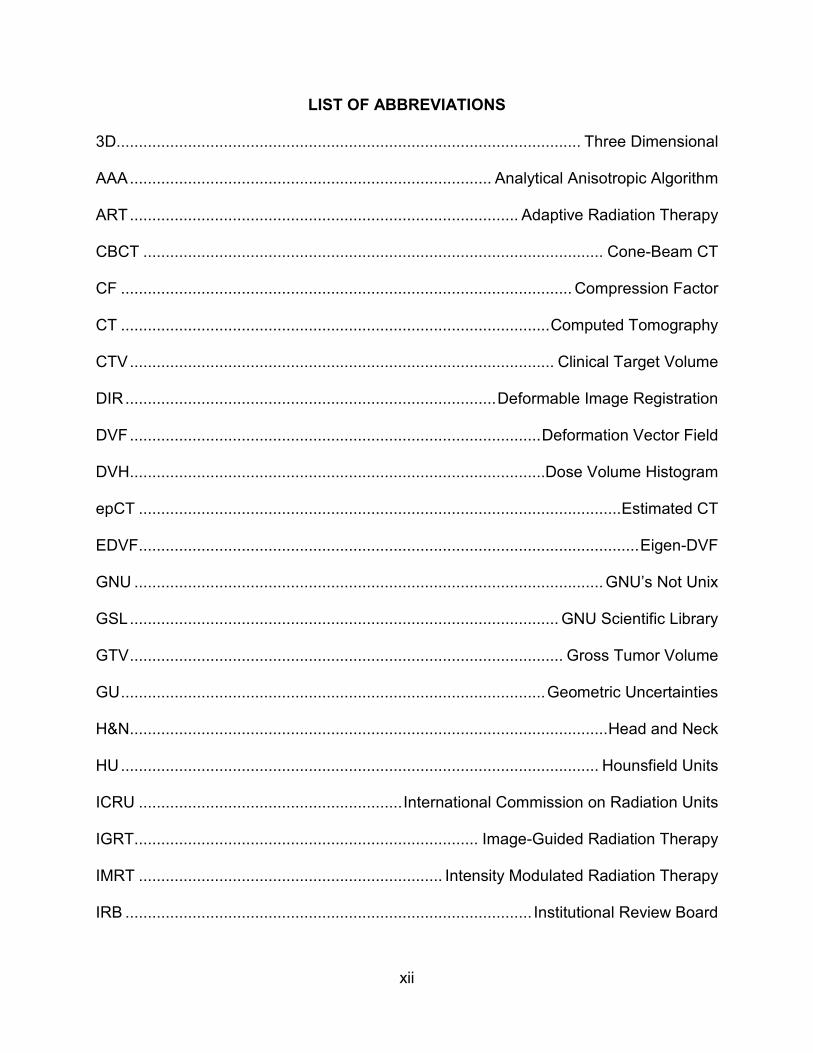
LIST OF ABBREVIATIONS

3D........................................................................................................ Three Dimensional

AAA ................................................................................. Analytical Anisotropic Algorithm

ART ....................................................................................... Adaptive Radiation Therapy

CBCT ....................................................................................................... Cone-Beam CT

CF ..................................................................................................... Compression Factor

CT ................................................................................................ Computed Tomography

CTV ............................................................................................... Clinical Target Volume

DIR ................................................................................... Deformable Image Registration

DVF ............................................................................................ Deformation Vector Field

DVH .............................................................................................Dose Volume Histogram

epCT ............................................................................................................ Estimated CT

EDVF ................................................................................................................ Eigen-DVF

GNU ......................................................................................................... GNU’s Not Unix

GSL ................................................................................................ GNU Scientific Library

GTV ................................................................................................. Gross Tumor Volume

GU ............................................................................................... Geometric Uncertainties

H&N ........................................................................................................... Head and Neck

HU ........................................................................................................... Hounsfield Units

ICRU ........................................................... International Commission on Radiation Units

IGRT ............................................................................. Image-Guided Radiation Therapy

IMRT .................................................................... Intensity Modulated Radiation Therapy

IRB ........................................................................................... Institutional Review Board

xiii

Linac ..................................................................................................... Linear Accelerator

NTCP .................................................................. Normal Tissue Complication Probability

OAR ............................................................................................................ Organ-at-Risk

OSG .......................................................................................... Organ Sample Generator

PC .................................................................................................... Principal Component

PCA .................................................................................... Principal Component Analysis

pCT ................................................................................................................ Planning CT

PRV ................................................................................................ Planning Risk Volume

PTV ............................................................................................. Planning Target Volume

RAM .......................................................................................... Random-Access Memory

QA ........................................................................................................ Quality Assurance

QUANTEC .............................Quantitative Analysis of Normal Tissue Effects in the Clinic

RPCA ............................................................. Regularized Principal Component Analysis

SPCA ................................................................. Standard Principal Component Analysis

TPS ....................................................................................... Treatment Planning System

wCT ................................................................................................................. Warped CT

1

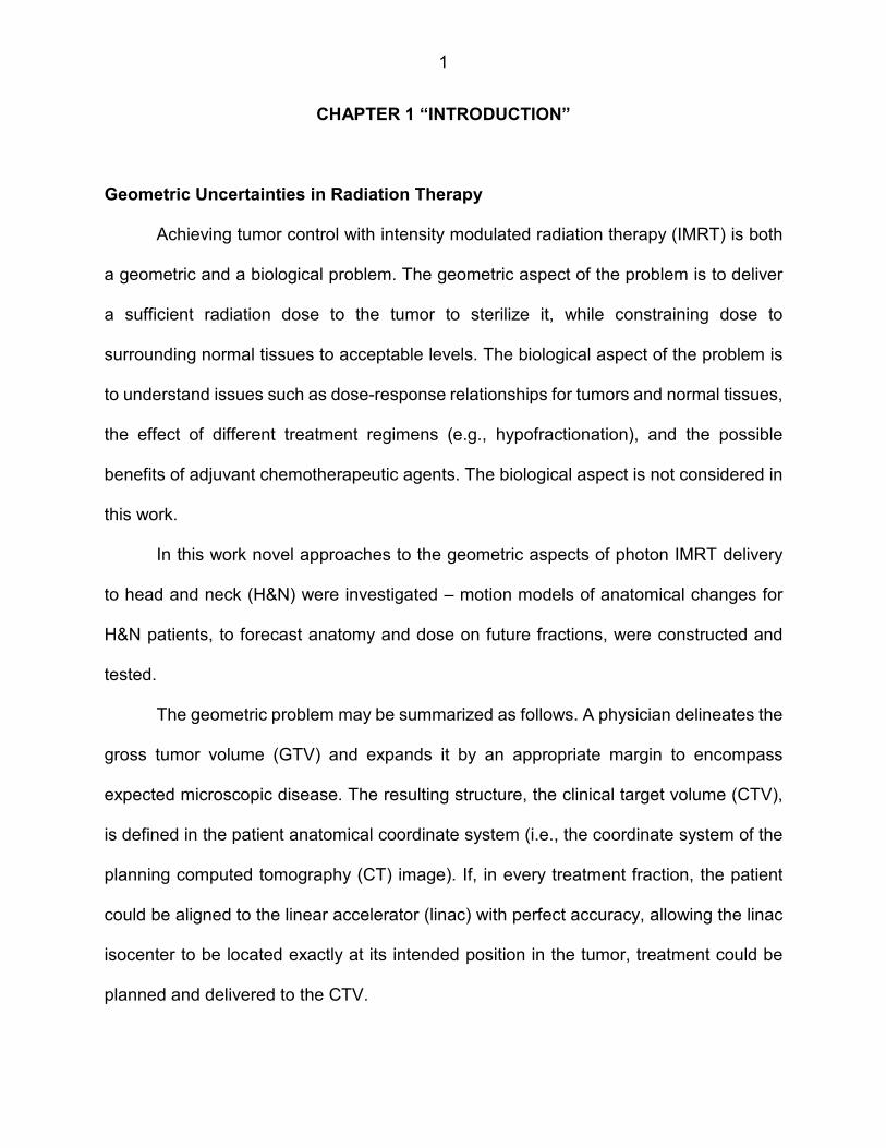
CHAPTER 1 “INTRODUCTION”

Geometric Uncertainties in Radiation Therapy

Achieving tumor control with intensity modulated radiation therapy (IMRT) is both

a geometric and a biological problem. The geometric aspect of the problem is to deliver

a sufficient radiation dose to the tumor to sterilize it, while constraining dose to

surrounding normal tissues to acceptable levels. The biological aspect of the problem is

to understand issues such as dose-response relationships for tumors and normal tissues,

the effect of different treatment regimens (e.g., hypofractionation), and the possible

benefits of adjuvant chemotherapeutic agents. The biological aspect is not considered in

this work.

In this work novel approaches to the geometric aspects of photon IMRT delivery

to head and neck (H&N) were investigated – motion models of anatomical changes for

H&N patients, to forecast anatomy and dose on future fractions, were constructed and

tested.

The geometric problem may be summarized as follows. A physician delineates the

gross tumor volume (GTV) and expands it by an appropriate margin to encompass

expected microscopic disease. The resulting structure, the clinical target volume (CTV),

is defined in the patient anatomical coordinate system (i.e., the coordinate system of the

planning computed tomography (CT) image). If, in every treatment fraction, the patient

could be aligned to the linear accelerator (linac) with perfect accuracy, allowing the linac

isocenter to be located exactly at its intended position in the tumor, treatment could be

planned and delivered to the CTV.

2

In reality, even when image guidance is used to carefully align the patient to the

linac, the patient’s intended position can still be offset from the isocenter1. Causes of

offsets include: (i) setup errors2 (imprecisions and inaccuracies inherent in the alignment

tools used to position the patient with respect to the linac at the start of each fraction),

and (ii) target (CTV) motion during delivery of each fraction3, 4. The above effects are

random — target shape and position assume different random values, characterized by

probability distributions, for each treatment course and fraction. Both effects create

uncertainty in the position of the isocenter, and are accordingly referred to as geometric

uncertainties (GUs).

Organ-at-risk (OAR) motion is a third category of GU5. At the start of a treatment

fraction, an OAR can be offset from the isocenter by a different amount than in the

planning CT (pCT), and can move relative to the isocenter (and CTV) during the fraction.

The planning implications of OAR setup uncertainty and motion are different than for

targets. One can reasonably hope to reduce target uncertainties through accurate (e.g.,

image-guided) setup. However, OAR motion is independent of the target, and cannot be

eliminated through target alignment.

Delineation uncertainty is a fourth category of GU6-8. Delineation of gross tumor

and organs-at-risk (OARs) on the planning CT is typically a manual operation subject to

physician judgment. Errors or uncertainties can occur as a result of poor quality images,

contouring shortcuts (such as contour interpolation across CT slices), time pressure on

physicians, or unconscious bias when e.g., the physician is overly conservative when

contouring targets in the vicinity of an OARs. Like setup uncertainties and tissue motion,

delineation errors create a degree of geometric uncertainty in the true position of targets

3

and OARs with respect to the linac, and can therefore be addressed using the same

planning techniques. Automated segmentation methods based on structure atlases9

have the potential to reduce delineation uncertainties, but residual errors persist even

with these methods.

Changes in patient anatomy during the course of radiation therapy (e.g. weight

loss, tumor shrinkage, lymph node shrinkage, etc.) represent a fifth category of GU. One

of the major reasons for such anatomical changes is the tissues’ response to the radiation,

causing e.g., tumor shrinkage, localized edema, etc. However, anatomical changes can

occur for other reasons, e.g. general weight loss due to change in eating habits.

Numerous research papers discuss importance of anatomical changes during radiation

therapy10-14.

The above five GUs should be considered during the treatment planning process

in order to accurately perform radiation therapy.

Conventional Method of Handling Geometric Uncertainties

The conventional method of accounting for uncertainties in the position of the CTV

relative to the linac (i.e., isocenter) is to expand the CTV to a planning target volume

(PTV), and plan treatment to the PTV. Beams are configured, and IMRT inverse planning

is performed, to ensure that in the static plan (i.e., the conventional plan generated prior

to the start of treatment using the pCT image) the entire PTV receives the prescription

dose (or a dose that is acceptably close to the prescription dose). In this case the PTV

represents a bounding envelope within which one expects to find the entire CTV for every

treatment fraction. This framework is described in ICRU reports 50 and 6215, 16.

4

The size of the CTV-to-PTV margin controls the tradeoff between target and

normal tissue doses. The margin needs to be large enough to ensure the CTV is covered

most of the time, but not significantly larger, since that can result in OARs receiving

unnecessary dose, leading to toxicity. The requirement that the CTV be covered (e.g.,

enclosed by the prescription dose isodose surface) “most of the time” is a coverage

criterion. In the widely-used margin formula proposed by van Herk et al17, “most of the

time” is made mathematically precise by interpreting it to mean “95% minimum dose to

CTV in 90% of patients”. However, alternative approaches to PTV margins are possible.

In clinical practice, margins are often set to round values such as 0.5 cm or 1.0 cm based

on clinical conventions. In that case, the margin is justified by pointing to prior clinical

experience that demonstrates generally acceptable treatment outcomes. There is a large

number of published studies investigating appropriate CTV-to-PTV margin size for

different treatment sites18-21.

Conventional Method of Handling OAR Uncertainties

In considering geometric uncertainties, much of the published literature focuses on

target coverage and CTV-to-PTV margins. The ICRU framework15, 16 also allows for

planning organ at risk volumes (PRVs) to be defined around OAR. The concept is similar

to that of a PTV. The OAR-to-PRV margin is intended to create a ‘buffer zone’ around the

OAR that can absorb geometric uncertainties. If OAR optimization criteria are applied to

the PRV instead of the OAR, those constraints should be respected in the presence of

geometric uncertainties.

5

However, practical application of PRVs is not straightforward. In the case of

targets, there is generally a single prescription dose to be applied uniformly across the

PTV. In that case, simple treatment models of the type used by van Herk et al.22 can be

used to estimate the amount by which the prescription dose isodose surface “pulls back”

towards the CTV, as a result of the cumulative blurring of beams over multiple fractions.

One can then compensate for this pull-back via the CTV-to-PTV margin.

For OARs there are typically multiple optimization criteria at different tolerance

doses. The effect of blurring on the corresponding isodose surfaces will vary according

to dose. For high doses, the isodose surface will pull back into the high dose region. For

lower doses, it may push out from the high dose region, closer to the OARs. Based on

the van Herk model, there is consequently no single OAR-to-PRV margin that will match

all dose-volume criteria. Stroom and Heijmen23 have investigated PRVs, concluding that

they change the underlying OAR volume “in such a manner that dose-volume constraints

stop making sense”. For these reasons, PRVs are not widely used in clinical practice.

The non-use of PRVs means that the effects of geometric uncertainties (e.g., organ

motion) on OAR are largely ignored. Failure to explicitly account for geometric

uncertainties is thought to be one barrier to acquiring reliable and clinically useful

biological outcomes models for OAR. The QUANTEC report24 summarizes clinical data

and models for a number of OAR. QUANTEC chapter 2025 discusses the need to record

“true dose” (i.e., dose delivered in the presence of geometric uncertainties) as opposed

to planned dose, stating that “only careful studies that include estimates of (true dose) will

allow us to confidently disentangle the effects of dosimetry and radiobiological sensitivity”.

6

Conventional Method of Handling Delineation Uncertainties

In conventional clinical planning, delineation uncertainties are mostly ignored. One

interpretation of current practice would be that delineation uncertainties are assumed to

be sufficiently small that they are safely absorbed within current GTV-to-CTV and CTV-

to-PTV margins, i.e., there is no need to explicitly account for them. However, the

evidence from inter- and intra-observer studies26-28 is that delineation uncertainties can

be large relative to typical margins. Furthermore, as time goes on, advances in treatment

delivery and imaging are reducing setup errors, and enabling organ motion to be

quantitatively modeled more accurately than was previously possible. For these reasons,

one can reasonably argue that delineation uncertainties need to be accurately quantified,

and explicitly accounted for in treatment planning7.

Role of Image-Guided Radiation Therapy and Adaptive Radiation Therapy in Handling Uncertainties

Image-guided radiation therapy (IGRT)29 largely focuses on more accurate tumor

targeting and tracking, and is less concerned with OAR motion. Recognizing that IGRT

cannot mitigate the effects of changes in tumor shape, or motion of OAR with respect to

the tumor, adaptive radiation therapy (ART)30, 31 provides a complementary strategy in

which the treatment plan is periodically updated throughout the treatment course. Both

IGRT and ART have the goal of reducing geometric uncertainties. ART is likely to be most

effective in cases where inter-fraction anatomic changes are significant with respect to

intra-fraction changes. ART can be performed offline or online, with online planning being

more effective, but more challenging due to the requirement to re-plan and perform quality

assurance within a narrow time window.

7

Motivation for Motion Model Development in Radiation Therapy for Head and Neck Patients

IMRT in H&N cancer conforms very precisely to the three-dimensional (3D) shape

of the tumor by modulating the intensity of the radiation beam in multiple small volumes.

IMRT also allows higher radiation doses to be focused to regions within the tumor while

minimizing the dose to surrounding normal critical structures32-35. Thus, the therapeutic

index can potentially be increased by using IMRT as opposed to classical 3D conformal

radiation therapy (RT).

However, conformal dose distributions are sensitive to GUs presented in patients,

like daily setup errors or changes in the anatomy during treatment course due to the

reasons mentioned above. For positional errors, online correction strategies like IGRT

can help to minimize the effects of systematic and random setup errors36-38. However,

residual setup uncertainties still exist and IGRT alone cannot compensate for non-rigid

deformations of the anatomy39.

ART is a potential solution for this problem. Although the concept of ART was

proposed more than a decade ago31, clinical implementation has lagged in part because

of the inability to answer practical questions such as: What anatomical changes are

important? How do we measure them? When to trigger re-planning? And how best to

perform the re-planning?

Statement of the Problem

Having models of anatomical changes over the course of treatment is essential to

answer the above questions. Models should take into account not only rigid body

transformations but also deformations, and be capable of extracting useful information

8

about changes in patient anatomy, ideally early in the radiation therapy course.

Several mathematical models have been proposed to account for patient motion40-

46. Among them, principal component analysis (PCA) was chosen in this study to model

anatomical changes47. PCA is potentially a powerful and efficient method and is capable

of identifying eigenmodes which are most responsible for the observed variations48. PCA

compresses large multidimensional and unorganized data to a low-dimensional system

of basis vectors (eigenvectors), representing major modes of anatomical change.

PCA models have been used for dosimetric evaluation of virtual prostate treatment

courses47, geometric coverage estimation49, lung deformation modeling50, automatic

organ segmentation51 and organ shape variability analysis52. However, to date, the

implementation of PCA models has not been utilized for extracting systematic changes in

patient anatomy during the H&N radiation therapy course. More information and material

about PCA will be introduced in Chapter 2.

This work presents initial results on PCA modeling for characterizing systematic

anatomical changes in H&N patients using daily cone-beam CT (CBCT) images. The goal

is to reliably identify systematic anatomical changes early in the treatment course, in order

to trigger re-planning decisions. A further goal is to capture normal tissue and tumor

changes for treatment response assessment.

9

CHAPTER 2 “STANDARD PRINCIPAL COMPONENT ANALYSIS MODEL OF ANATOMICAL CHANGES IN HEAD AND NECK PATIENTS”

Introduction

The central idea of principal component analysis (PCA) is to reduce the

dimensionality of a data set consisting of a large number of interrelated variables, while

retaining as much as possible of the variation present in the data set48. To achieve this

PCA performs orthonormal transformation of an original data set to a new set of variables

called principal components (PC), which are orthonormal, and therefore uncorrelated to

each other. The first PC is defined in such a way that it accounts for the largest possible

variability in the data, while each succeeding PC in turn has the largest possible variability

under the constraint that it is orthogonal to all preceding PCs.

PCA was first introduced in 1901 by K. Pearson53. Since then it became a handy

tool which is used widely in predictive modeling.

This chapter discusses the develop of standard PCA (SPCA) models of anatomical

change from daily CBCTs of H&N patients, and assesses the possibility of using these in

adaptive radiation therapy and to extract quantitative information for treatment response

assessment.

Materials and Methods

Clinical and Simulated Image Data

Ten H&N patients with daily CBCT imaging were retrospectively selected under an

Institutional Review Board (IRB) approved protocol. Each patient experienced different

systematic changes during the course of radiotherapy, like parotid shrinkage, weight loss,

10

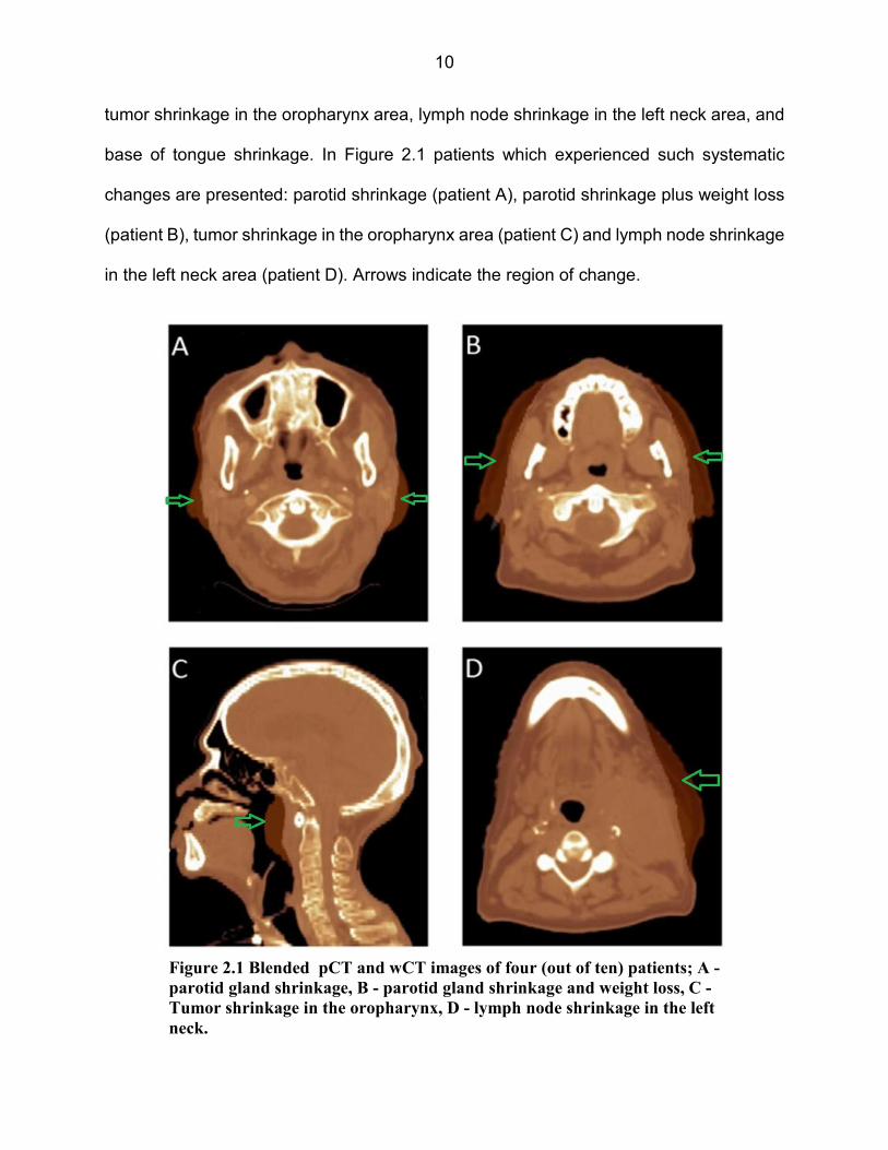
tumor shrinkage in the oropharynx area, lymph node shrinkage in the left neck area, and

base of tongue shrinkage. In Figure 2.1 patients which experienced such systematic

changes are presented: parotid shrinkage (patient A), parotid shrinkage plus weight loss

(patient B), tumor shrinkage in the oropharynx area (patient C) and lymph node shrinkage

in the left neck area (patient D). Arrows indicate the region of change.

Figure 2.1 Blended pCT and wCT images of four (out of ten) patients; A -

parotid gland shrinkage, B - parotid gland shrinkage and weight loss, C -

Tumor shrinkage in the oropharynx, D - lymph node shrinkage in the left

neck.

11

For each patient, a synthetic warped CT (wCT) was generated from the pCT image

using an in-house developed interactive software tool. The interface of this tool is shown

in Figure 2.2.

The goal of the warping was to simulate the predominant localized systematic

anatomical change over the duration of the patient treatment (Figure 2.1, arrows). So, for

patient A, for example, the sole difference between the pCT and wCT was the deformation

of the parotids and immediately adjacent tissue. Away from the parotids, the pCT and

wCT matched exactly. The interactive warping tool was developed in Matlab®

(MathWorks Inc., Natick, MA). It incorporated the barrel distortion function54 and pencil

tool, and allowed the user to iteratively expand, contract and shape a region of the pCT

anatomy using a computer mouse. The generated wCTs were inspected by a radiation

oncologist with expertise in H&N to ensure clinical realism.

The generated wCTs constitute digital phantoms, allowing PCA results to be

evaluated in a controlled setting where the exact nature of anatomical change is known

Figure 2.2 In-house developed interactive software tool (Matlab®) to perform warping of the

images

12

a priori. Results below compare PCA’s ability to extract anatomical change from digital

phantoms (specifically, synthetic CBCTs generated from the wCT), as well as from real

patients (i.e., clinical CBCTs). For clinical images, anatomical change is not known a priori

and likely contains a variety of random components due to fraction-to-fraction setup

uncertainties, posture variations, etc. Clinical images and deformation vector fields

(DVFs) are therefore expected to be a greater challenge for the PCA technique.

Deformation Vector Fields Data

Prior to DVF generation, clinical or synthetic CBCT images were rigidly aligned

with pCTs using bony skull and C2-C3 cervical vertebrae, to ensure all DVFs were relative

to the fixed skull. The pCTs acted as reference imaged. DVFs were generated and

manipulated in the Pinnacle® Treatment Planning System (TPS), utilizing Pinnacle

plugins in conjunction with the open source GNU Scientific Library (GSL)55 for matrix

operations. DVFs for all patients were generated using Pinnacle’s diffeomorphic demons

algorithm56-58. A compression factor (CF) of 7 was used, meaning that a single DVF voxel

covers 7 CT voxels (~ 7 mm) in the coronal and sagittal (X and Y) directions. This was

done in order to keep PCA model generation numerically feasible. DVF voxel size in the

axial (Z) direction was 3mm independent of the CF.

DVFs were restricted to a bounding box of the approximate size of the patient head

and neck in order to speed up calculation. Bounding boxes were set sufficiently large to

accommodate all anatomies. DVF values were set to zero for voxels outside the (pCT)

patient body to avoid spurious deformations that are an artifact of the deformable image

registration (DIR) algorithm. Given the number of voxels M, a DVF in 3D space is

13

represented as a vector of length 3M, representing X, Y and Z displacements.

It is worth noting the mathematical conventions that apply to DVFs. Each DVF is

defined between a fixed image and a moving image. In the present case, the fixed image

is the pCT, and the moving image is the wCT or CBCT. The DVF is defined on (i.e., is the

same size as) the voxel grid in the fixed image. However, as explained by Yang59, the

DVF is a pull-back motion field. Each element of the DVF is a 3D vector (arrow) from a

point in the fixed image to the matching point in the moving image. Consequently, one

‘applies’ the DVF to the moving image (wCT or CBCT) to recover the fixed image (pCT).

In visual terms, given the moving image, one “pulls back” tissue volumes at arrow tips to

the corresponding arrow bases, to recover the fixed image.

Clinical Deformation Vector Fields

In the following description a patient’s ith CBCT is denoted CBCTi. Clinical DVFs

were generated as follows:

�,� = �����→�����

DC,i denotes the clinical DVF from pCT to CBCTi. It models systematic plus random

change from planning to fraction i. The differential DVF, which models the motion

difference between two successive fractions, is defined as follows:

�,� = �,� − �,���

In the case of clinical images, the final available CBCT for the patient was regarded

as the end-of-treatment anatomy (similar to the wCT).

Synthetic Deformation Vector Fields

14

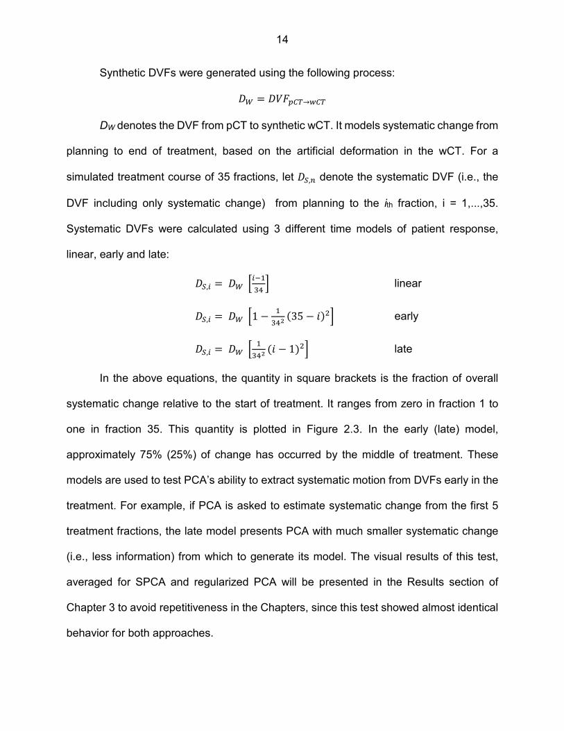
Synthetic DVFs were generated using the following process:

� = �����→���

DW denotes the DVF from pCT to synthetic wCT. It models systematic change from

planning to end of treatment, based on the artificial deformation in the wCT. For a

simulated treatment course of 35 fractions, let �,� denote the systematic DVF (i.e., the

DVF including only systematic change) from planning to the ith fraction, i = 1,...,35.

Systematic DVFs were calculated using 3 different time models of patient response,

linear, early and late:

�,� = � ���� ! " linear

�,� = � �1 − � !# $35 − &'(" early

�,� = � � � !# $& − 1'(" late

In the above equations, the quantity in square brackets is the fraction of overall

systematic change relative to the start of treatment. It ranges from zero in fraction 1 to

one in fraction 35. This quantity is plotted in Figure 2.3. In the early (late) model,

approximately 75% (25%) of change has occurred by the middle of treatment. These

models are used to test PCA’s ability to extract systematic motion from DVFs early in the

treatment. For example, if PCA is asked to estimate systematic change from the first 5

treatment fractions, the late model presents PCA with much smaller systematic change

(i.e., less information) from which to generate its model. The visual results of this test,

averaged for SPCA and regularized PCA will be presented in the Results section of

Chapter 3 to avoid repetitiveness in the Chapters, since this test showed almost identical

behavior for both approaches.

15

Random changes were added to the synthetic DVFs as follows. Random DVFs DR

were modeled as scaled linear combinations of the DDC,i : ) = * ∑ ,� �,�� , where

,�- .0,10 are uniformly distributed random weights summing to one, which vary from

fraction to fraction, and * is a scaling parameter taking the values 1, 3 or 5, that is fixed

for each treatment course. The case * = 1 approximates the magnitude of random

motion present in clinical CBCTs. Cases * = 3 12 5 artificially increase the magnitude of

random motion, to test PCA’s ability to extract systematic changes in the presence of

increased random motion.

Finally, the synthetic DVF DSR,i for fraction i, incorporating both systematic and

Figure 2.3 Early, linear and late models of patient response

16

random changes, was defined as follows:

�),� = �,� + ) = �,� + * ∑ ,� �,�� (2.1)

Note that DR varies from fraction to fraction and between simulated treatment

courses, as determined by the random number generator. In equation 2.1, the + symbol

indicates element-by-element addition of DVFs.

PCA Models – Standard PCA

This section describes the generation of a patient-specific SPCA model. Let D =

[D1, ..., DF] be an 3M x F matrix, whose column Df is a DVF of length 3M, where M is the

total number of voxels. In a clinical scenario, Df is the DVF from the planning CT to the

fraction f CBCT, f = 1, 2, ..., f ≤ N, where N is the number of fractions in the treatment

course. Input data for PCA modeling is typically made zero-mean by first subtracting the

mean DVF. Without loss of generality, we assume that the mean DVF 4 has already been

subtracted from each of the Df . DVFs from the first F fractions are used to build a model

that can be used to predict anatomical changes for the remaining fractions. Let E = [E1,

..., EF] be an 3M x F matrix, whose columns Ef are eigenvectors, here referred as

eigenDVFs (EDVFs). PCA solves the following constrained optimization problem for E:

min8 ‖ : − ;;<: ‖ subject to ;<; = => (2.2)

where IF is the F x F identity matrix and, for arbitrary matrix ? = @A��B, ‖∙‖ is the Frobenius

norm: ‖?‖ = DE2F G∑ A��(�,� H. The solution of equation 2.2 is a set of orthonormal EDVFs

Ef, each of which is derived from an eigenvector of the covariance matrix I = :<:/M. The

solution E can be obtained by using standard matrix operations to find the eigenvalues

and eigenvectors of C. Further details about matrix operations used in this work to build

17

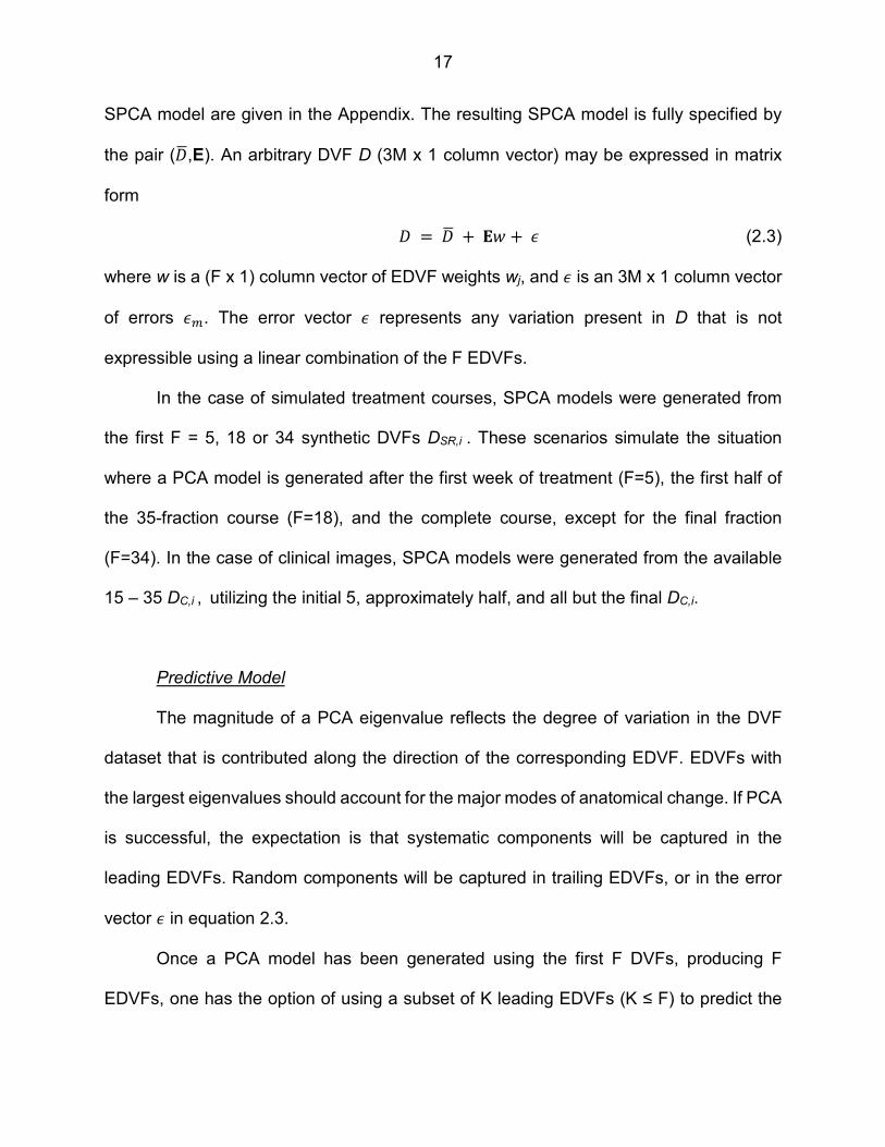
SPCA model are given in the Appendix. The resulting SPCA model is fully specified by

the pair ( 4,E). An arbitrary DVF D (3M x 1 column vector) may be expressed in matrix

form

= 4 + ;� + - (2.3)

where w is a (F x 1) column vector of EDVF weights wj, and - is an 3M x 1 column vector

of errors -K. The error vector - represents any variation present in D that is not

expressible using a linear combination of the F EDVFs.

In the case of simulated treatment courses, SPCA models were generated from

the first F = 5, 18 or 34 synthetic DVFs DSR,i . These scenarios simulate the situation

where a PCA model is generated after the first week of treatment (F=5), the first half of

the 35-fraction course (F=18), and the complete course, except for the final fraction

(F=34). In the case of clinical images, SPCA models were generated from the available

15 – 35 DC,i , utilizing the initial 5, approximately half, and all but the final DC,i.

Predictive Model

The magnitude of a PCA eigenvalue reflects the degree of variation in the DVF

dataset that is contributed along the direction of the corresponding EDVF. EDVFs with

the largest eigenvalues should account for the major modes of anatomical change. If PCA

is successful, the expectation is that systematic components will be captured in the

leading EDVFs. Random components will be captured in trailing EDVFs, or in the error

vector - in equation 2.3.

Once a PCA model has been generated using the first F DVFs, producing F

EDVFs, one has the option of using a subset of K leading EDVFs (K ≤ F) to predict the

18

major mode of anatomical change for subsequent fractions. If, for example, there is only

one major mode of anatomical change (e.g., tumor shrinkage), and that mode is captured

in the first EDVF, then a satisfactory predictive model may be achieved using K = 1.

Additionally, the PCA modeling process makes no assumptions regarding how

major modes of motion evolve during treatment. PCA EDVFs capture the direction but

not the time-varying magnitude of anatomical changes. After generation of the PCA

model, observed DVFs can be expressed as a linear combination of EDVFs (equation

(2.3), where the weights w will in general vary as treatment progresses. The trajectory of

weights w will indicate whether treatment response is early, linear or late, as in Fig. 2.3.

The default predictive model given below makes the assumption that evolution is linear.

However, this approach can be generalized to model early or late response, provided one

has sufficient knowledge to justify those models.

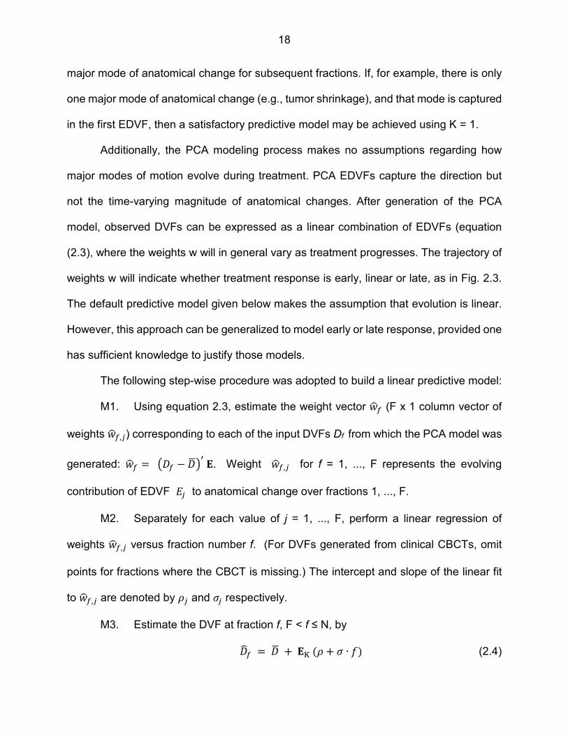
The following step-wise procedure was adopted to build a linear predictive model:

M1. Using equation 2.3, estimate the weight vector ��� (F x 1 column vector of

weights ���,�) corresponding to each of the input DVFs Df from which the PCA model was

generated: ��� = G � − 4H< ;. Weight ���,� for f = 1, ..., F represents the evolving

contribution of EDVF L� to anatomical change over fractions 1, ..., F.

M2. Separately for each value of j = 1, ..., F, perform a linear regression of

weights ���,� versus fraction number f. (For DVFs generated from clinical CBCTs, omit

points for fractions where the CBCT is missing.) The intercept and slope of the linear fit

to ���,� are denoted by M� and N� respectively.

M3. Estimate the DVF at fraction f, F < f ≤ N, by

O� = 4 + ;P $M + N ∙ Q' (2.4)

19

where M and N are the K x 1 column vectors of M� and N�, and EK is the 3M x K

matrix, whose columns Ej are the first K EDVFs.

The relationship between measured DVFs (i.e., input DVFs Df in step M1) and

predicted DVFs (output DVFs from equation 2.4) is illustrated in Figure 2.4. The

orientation of DVF arrows is from fixed image to moving image, enabling CBCTs to be

mapped to the pCT. In principle, these DVFs can be inverted to give DVFs that will map

the pCT to predicted CBCTs for fractions F+1, ..., N. PCA-predicted DVFs are evaluated

using criteria outlined in the next section.

Model Evaluation

A hypothesis of this study is that the PCA model can successfully separate

systematic from random anatomical changes, capturing systematic changes in a few

leading EDVFs. One indicator of success is that, in step M2 above, the weights ���,�

associated with leading EDVFs exhibit non-zero slopes N�, high R2 values and, more

pCT

CBCT1 . . . CBCTF

CBCTF+1 CBCTN . . .

wCT

PCA model from first F

clinical DVFs

Measured

DVFs

PCA predicted

DVFs & CBCTs

Figure 2.4 Relationship between measured and predicted DVFs

CBCTF+1 CBCTN

clinical CBCTs

20

generally, smooth and consistent evolution with fraction number f. Conversely, weights

���,� associated with trailing EDVFs should exhibit near-zero slopes, low R2, and purely

random variation with fraction number f. A further qualitative indicator of PCA success is

that the areas where leading EDVFs are non-zero are restricted to localized parts of the

anatomy where systematic changes are occurring.

PCA models may also be evaluated quantitatively. This can be done by using the

PCA model to warp the end-of-treatment anatomy to the predicted anatomy at the time

of simulation. In this way one obtains an estimated planning CT, or epCT. Then one can

compare epCT with the true planning CT (pCT) to assess how well the PCA model

reproduces anatomical changes during treatment. The specific steps for generating epCT

are:

S1. For simulated treatments, apply O R from equation 2.4 to the wCT to get

epCT.

S2. For clinical CBCT images, let fE denote the fractions of the final CBCT

image. Apply O�S from equation (4) to CBCT�Sto get epCT.

Agreement between the pCT and epCT quantifies the difference between the real

and estimated planning anatomies ‖pCT − epCT‖. Note that the PCA model is intended

to capture only systematic anatomical changes. The end-of-treatment anatomy, from

which epCT is generated, will also incorporate random changes. Consequently, the

difference metric ‖pCT − epCT‖ will reflect how well PCA does at extracting the

systematic component of anatomical change, but it will also reflect the effect of random

anatomical changes not included in the model, and DIR uncertainties inherent in the DVFs

used to construct the PCA model. Finally, in the case of the clinical CBCT images, epCT

21

is obtained by applying a modeled DVF to the end-of-treatment CBCT. Consequently, in

this case epCT will include an increased level of noise inherent in CBCT (versus CT)

images. This also will tend to increase the value of ‖pCT − epCT‖.

We define images error vector LY as the difference between pCT and epCT

images:

LY = Z[\ − ]Z[\Y (2.5)

where epCTF is the estimated CT obtained from the PCA model that is generated from

the first F fractions DVFs. LY is a vector of length M. Each element of LY is the error in

the estimated CT number for the corresponding voxel.

For PCA models based on clinical CBCTs, where one is limited to the available

CBCTs, we define the patient-specific distance metric to be the root mean square CT

number difference:

‖Z[\ − ][\Y‖ = ^ �_ ∑ $LY'(_a� (2.6)

For PCA models based on synthetic CBCT images generated from wCT, it is

possible to perform S simulations, where each simulation generates a different realization

of random changes throughout the treatment course. In this case we define the patient-

specific distance metric to be the root mean square CT number difference, averaged over

simulations:

‖Z[\ − ][\Y‖ = �� ∑ ^ �

_ ∑ $LY'(_a��ba� (2.7)

In addition to these distance metrics, 3D gamma indices60 were calculated

between pCT and epCT images using 3% / 3mm criteria (3% difference in Hounsfield

Units (HU), and 3mm distance-to-agreement). ‖pCT − epCT‖ and gamma values were

22

calculated for PCA models generated using the first five fractions, half of the treatment

fractions, and all but last treatment fraction.

Results

Qualitative Evaluation

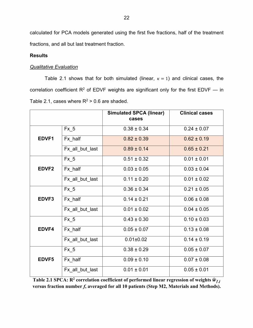
Table 2.1 shows that for both simulated (linear, * = 1) and clinical cases, the

correlation coefficient R2 of EDVF weights are significant only for the first EDVF — in

Table 2.1, cases where R2 > 0.6 are shaded.

Simulated SPCA (linear) cases

Clinical cases

EDVF1

Fx_5 0.38 ± 0.34 0.24 ± 0.07

Fx_half 0.82 ± 0.39 0.62 ± 0.19

Fx_all_but_last 0.89 ± 0.14 0.65 ± 0.21

EDVF2

Fx_5 0.51 ± 0.32 0.01 ± 0.01

Fx_half 0.03 ± 0.05 0.03 ± 0.04

Fx_all_but_last 0.11 ± 0.20 0.01 ± 0.02

EDVF3

Fx_5 0.36 ± 0.34 0.21 ± 0.05

Fx_half 0.14 ± 0.21 0.06 ± 0.08

Fx_all_but_last 0.01 ± 0.02 0.04 ± 0.05

EDVF4

Fx_5 0.43 ± 0.30 0.10 ± 0.03

Fx_half 0.05 ± 0.07 0.13 ± 0.08

Fx_all_but_last 0.01±0.02 0.14 ± 0.19

EDVF5

Fx_5 0.38 ± 0.29 0.05 ± 0.07

Fx_half 0.09 ± 0.10 0.07 ± 0.08

Fx_all_but_last 0.01 ± 0.01 0.05 ± 0.01

Table 2.1 SPCA: R2 correlation coefficient of performed linear regression of weights c� d,e versus fraction number f, averaged for all 10 patients (Step M2, Materials and Methods).

23

For EDVFs 2-5, R2 coefficients are generally much lower. For simulated cases, R2

values for EDVFs 2-5 in the 5-fraction PCA models (Fx_5) are higher (0.36 – 0.51). But

those R2 values drop substantially when more DVFs (fractions) are included in the PCA

models, indicating that EDVFs 2-5 are not reliably capturing systematic changes. Based

on Table 2.1, PCA models in this work utilize only one, or at most several, leading EDVFs.

For synthetic CBCTs, the estimated anatomy epCT at the time of simulation was

reconstructed by applying O R (equation 2.4) to the wCT image. Figure 2.5 shows results

for patient D, for whom PCA gave the best results (out of the 10 patients studied). Figure

2.6 shows results for patient A, for whom PCA gave the worst results. In each case, top

panels show pCT (red) overlaid on the epCT (green). The left-most panel (A) is for a PCA

Figure 2.5 SPCA: Results of SPCA models generated from synthetic DVFs for patient D, for

whom PCA modeling gave the best results

24

model constructed from the first 5 treatment fractions. The middle panel (B) is for a PCA

model constructed from the first 18 treatment fractions. The right-most panel (C) is for a

PCA model constructed from all but the last treatment fraction. Lower panels in Figures

2.5 and 2.6 show the projections of all 35 simulated DVFs onto the leading EDVF. The

error bars represent ± one standard deviation of EDVF weight values across simulated

treatment courses having different random motion components. To generate these

results, 10 different treatment courses were simulated for each patient.

Quantitative Evaluation

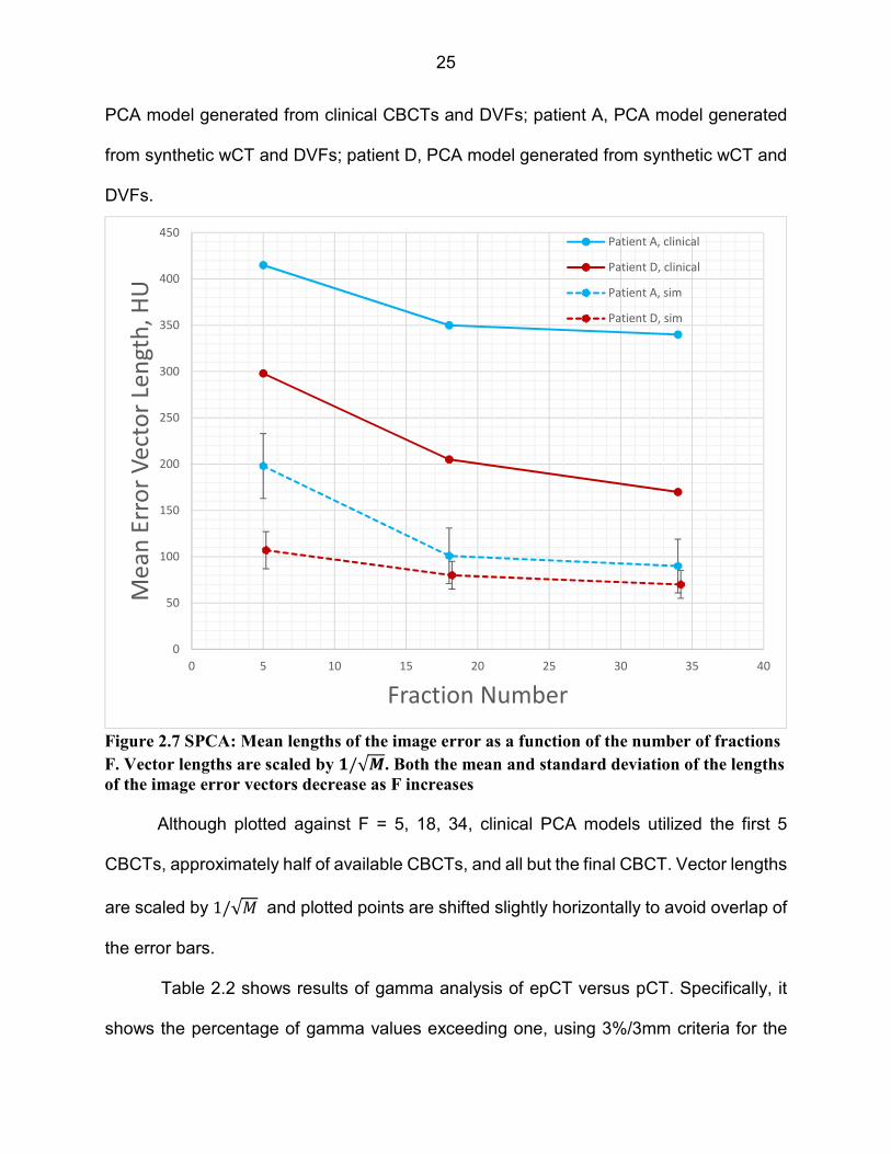
Figure 2.7 plots mean lengths of the image error vectors,‖pCT − epCT‖, equations

(2.6) and (2.7), as a function of the number of fractions F from which the PCA model is

generated: Patient A, PCA model generated from clinical CBCTs and DVFs; patient D,

Figure 2.6 SPCA: Results of SPCA models generated from synthetic DVFs for patient A, for

whom PCA modeling gave the worst results

25

PCA model generated from clinical CBCTs and DVFs; patient A, PCA model generated

from synthetic wCT and DVFs; patient D, PCA model generated from synthetic wCT and

DVFs.

Although plotted against F = 5, 18, 34, clinical PCA models utilized the first 5

CBCTs, approximately half of available CBCTs, and all but the final CBCT. Vector lengths

are scaled by 1/√ and plotted points are shifted slightly horizontally to avoid overlap of

the error bars.

Table 2.2 shows results of gamma analysis of epCT versus pCT. Specifically, it

shows the percentage of gamma values exceeding one, using 3%/3mm criteria for the

Figure 2.7 SPCA: Mean lengths of the image error as a function of the number of fractions

F. Vector lengths are scaled by f/√g. Both the mean and standard deviation of the lengths

of the image error vectors decrease as F increases

0

50

100

150

200

250

300

350

400

450

0 5 10 15 20 25 30 35 40

Me

an

Err

or

Ve

cto

r Le

ng

th,

HU

Fraction Number

Patient A, clinical

Patient D, clinical

Patient A, sim

Patient D, sim

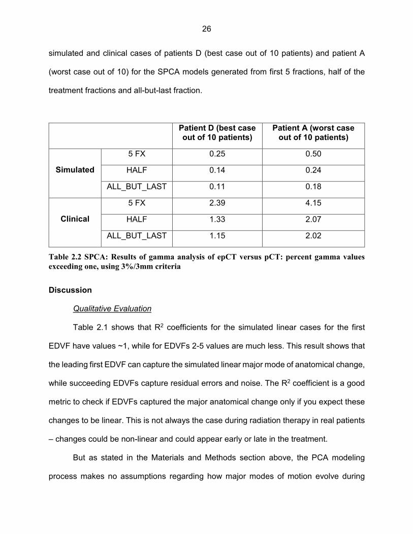
26

simulated and clinical cases of patients D (best case out of 10 patients) and patient A

(worst case out of 10) for the SPCA models generated from first 5 fractions, half of the

treatment fractions and all-but-last fraction.

Patient D (best case out of 10 patients)

Patient A (worst case out of 10 patients)

Simulated

5 FX 0.25 0.50

HALF 0.14 0.24

ALL_BUT_LAST 0.11 0.18

Clinical

5 FX 2.39 4.15

HALF 1.33 2.07

ALL_BUT_LAST 1.15 2.02

Discussion

Qualitative Evaluation

Table 2.1 shows that R2 coefficients for the simulated linear cases for the first

EDVF have values ~1, while for EDVFs 2-5 values are much less. This result shows that

the leading first EDVF can capture the simulated linear major mode of anatomical change,

while succeeding EDVFs capture residual errors and noise. The R2 coefficient is a good

metric to check if EDVFs captured the major anatomical change only if you expect these

changes to be linear. This is not always the case during radiation therapy in real patients

– changes could be non-linear and could appear early or late in the treatment.

But as stated in the Materials and Methods section above, the PCA modeling

process makes no assumptions regarding how major modes of motion evolve during

Table 2.2 SPCA: Results of gamma analysis of epCT versus pCT: percent gamma values

exceeding one, using 3%/3mm criteria

27

treatment – it’s just metric we use to evaluate it (like R2 for the linear changes). PCA

EDVFs capture the direction but not the magnitude of anatomical changes. Therefore,

using proper metrics (i.e. splines or polynomials) it is possible to check if EDVFs captured

major anatomical changes for non-linear cases. The results and discussion supporting

this statement are presented in Chapter 3.

Figure 2.5 shows that, given the right conditions, SPCA modeling is capable of

extracting the major mode of anatomical change during head and neck radiation therapy.

The leading EDVF coefficients show a smooth progression during treatment, and the

more CBCTs that are included in the SPCA model, the better the model becomes. This

is indicated by a progressive tightening of the standard deviations of EDVF weights as

one moves from model A (5 fractions), to model B (18 fractions), to model C (34 fractions).

In Figure 2.5 the modeled anatomical change, left neck lymph node shrinkage, is

large — it affects a relatively large volume of the patient’s anatomy. SPCA searches for

EDVFs that can explain variability across CBCT images. If the modeled anatomical

change is large, the SPCA technique is more easily able to ‘extract’ the major deformation

mode(s) from noisy data. This explains why patient D has the best PCA model across the

ten sampled patients.

In Figure 2.6 (patient A), the modeled anatomical change, bilateral parotid

shrinkage, is relatively small — it affects a localized volume around the parotids. In this

case SPCA finds it more difficult to isolate the anatomical change from other random

variations that are present in the CBCT images. For this reason, the SPCA model is not

as good as for patient D. The PCA models for F=5 and F=18 fractions show a fairly weak

linear progression of the leading EDVF coefficient, and the standard deviation of the

28

coefficients is large, indicating that the SPCA technique is having a difficult time ‘locking

onto’ the major deformation mode. Only when the treatment course is almost complete

(column C, F=34) does the SPCA model become good enough to predict the anatomy,

with a higher level of confidence.

One of the conclusions of this study is that SPCA — i.e., PCA applied directly to

DVFs without any further enhancement or refinement — will find it difficult to extract

smaller systematic anatomical changes from daily CBCT images. Where changes are

small, SPCA will tend to be confused by other random motion present in the images, and

the resulting PCA models will have diminished ability to predict or extrapolate anatomical

changes.

Quantitative Evaluation

Figure 2.7 shows that larger HU errors occur for the SPCA models generated from

clinical CBCTs (lines (a) and (b)), than those generated from synthetic images and DVFs

(lines (c) and (d)). Synthetic DVFs were generated artificially by inserting one known

anatomical change into the planning CT. Regions of the patient anatomy that were not

affected by the change were identical throughout the treatment course, except for added

random changes. This represents a best-case scenario for SPCA modeling. Having only

one systematic change present in the images makes it easier for the SPCA method to

capture that change within the leading EDVF.

Clinical CBCTs may include several types of systematic anatomical change — for

example, lymph node shrinkage in conjunction with weight loss. Clinical CBCTs can also

include random motion of the anatomy outside of the region directly involved in the

29

systematic change. Finally, evolution of the systematic change in clinical CBCTs may not

follow a simple linear progression, as was the case with the synthetic DVFs. For these

reasons, SPCA finds it more difficult to extract useful models from clinical CBCT images.

This conclusion is reinforced by the gamma results in Table 2.2. Those results

show that the number of voxels in epCT that disagree with pCT by more than 3% or 3

mm is fairly modest for the SPCA models generated from synthetic DVFs, but much larger

in models generated from clinical CBCTs.

Quantitative results shown in Figure 2.7 and Table 2.2 may be used as an indirect

way of testing the accuracy of DVFs, or the accuracy of the reconstructed epCT (acquired

by applying the last-fraction DVF from equation 2.4 to the pCT image) versus the pCT

image. Although thorough testing of DVFs accuracy was out of the scope of this work,

results of the quantitative analysis give an idea of how the number of fractions used to

build a model and random changes presented in simulated and clinical data affect the

quality of the last-fraction DVF and overall accuracy of the epCT with respect to the pCT

image.

Within this work we evaluated whether SPCA models generated from clinical

CBCTs could potentially be improved by including more than one leading EDVF. That is,

using K ≥ 2 as explained in the Predictive Model section above. However, for clinical

SPCA models the R2 coefficient was moderately good for the leading EDVF, but quite

poor for EDVFs 2-5 (see Table 2.1), indicating that there was no improvement derived

by including any EDVFs beyond the first. The conclusion of this work is that, particularly

for smaller anatomical changes, SPCA becomes ‘confused’ by the variety of deformations

and noise in clinical CBCT images, and therefore fails to extract major modes of

30

systematic change that are known to be present. In order to successfully model

anatomical change in clinical CBCT images, the basic SPCA technique will need to be

refined.

In Chapter 3 more extensive discussion about SPCA model and its comparison to

more advanced regularized PCA (RPCA) model will be presented.

Conclusion

For the H&N patients treated with external beam radiation therapy, a SPCA model

is a potential tool to identify patient anatomy changes early in the treatment course, and

to make educated adaptive re-planning decisions. This study used synthetic (but realistic)

DVFs, as well as clinical CBCTs, to evaluate the ability of the SPCA method to extract

useful models of anatomical change. In particular, a primary goal of this work was to

evaluate the ability of SPCA to separate systematic from random changes present in

CBCT images.

The study shows that under the right conditions, SPCA can capture the major

mode of systematic anatomical deformation in the leading EDVF. However, SPCA is most

successful at identifying large changes (e.g., significant lymph node shrinkage), and less

successful at identifying small changes (e.g., smaller changes in parotid glands).

Additionally, SPCA is challenged by the variety of deformations and noise in clinical CBCT

images, and therefore fails to extract major modes of systematic change that are known

to be present. In order to successfully model anatomical change in clinical CBCT images,

the basic SPCA technique will be refined using the regularized approach described in

Chapter 3.

31

CHAPTER 3 “REGULARIZED PRINCIPAL COMPONENT ANALYSIS MODEL OF ANATOMICAL CHANGES IN HEAD AND NECK PATIENTS”

Introduction

The purpose of this Chapter is to reveal, building on the Materials and Methods

section presented in Chapter 2, the details of developing regularized PCA (RPCA) models

of anatomical changes from daily CBCTs images of H&N patients, and assess their

potential use in ART, and for extracting quantitative information for treatment response

assessment.

The general motivation to build the RPCA model is the same as for the SPCA (i.e.,

modeling of anatomical change, see the Introduction section in Chapter 2). The specific

motivation is to improve on the SPCA results given in Chapter 2.

Materials and Methods

The dataset, DVFs and predictive model used to build the RPCA model are the

same as described in Chapter 2. The difference is in the constraint optimization problem

(equation 2, Chapter 2) one needs to solve to get EDVFs.

PCA Models – Regularized PCA

For reasons discussed below, standard PCA (SPCA) can produce EDVFs that are

noisy and not physically meaningful. RPCA offers a solution for this problem. The method

of generation of a patient-specific regularized RPCA model is similar to the SPCA model

described earlier. The difference lies in the constrained optimization problem for E that

PCA needs to solve for the regularized PCA approach:

32

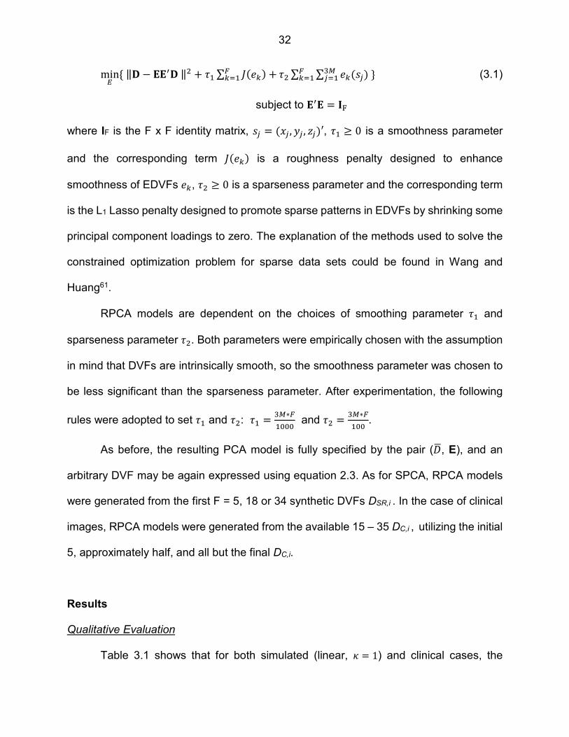
min8 { ‖: − ;;<: ‖( + i� ∑ j$]`' +Ya� i( ∑ ∑ ]`$D�' _�a�Ya� } (3.1)

subject to ;<; = =>

where IF is the F x F identity matrix, D� = $A� , l� , m�'′, i� ≥ 0 is a smoothness parameter

and the corresponding term j$]`' is a roughness penalty designed to enhance

smoothness of EDVFs ]`, i( ≥ 0 is a sparseness parameter and the corresponding term

is the L1 Lasso penalty designed to promote sparse patterns in EDVFs by shrinking some

principal component loadings to zero. The explanation of the methods used to solve the

constrained optimization problem for sparse data sets could be found in Wang and

Huang61.

RPCA models are dependent on the choices of smoothing parameter i� and

sparseness parameter i(. Both parameters were empirically chosen with the assumption

in mind that DVFs are intrinsically smooth, so the smoothness parameter was chosen to

be less significant than the sparseness parameter. After experimentation, the following

rules were adopted to set i� and i(: i� = _∗Y�qqq and i( = _∗Y

�qq .

As before, the resulting PCA model is fully specified by the pair ( 4, E), and an

arbitrary DVF may be again expressed using equation 2.3. As for SPCA, RPCA models

were generated from the first F = 5, 18 or 34 synthetic DVFs DSR,i . In the case of clinical

images, RPCA models were generated from the available 15 – 35 DC,i , utilizing the initial

5, approximately half, and all but the final DC,i.

Results

Qualitative Evaluation

Table 3.1 shows that for both simulated (linear, * = 1) and clinical cases, the

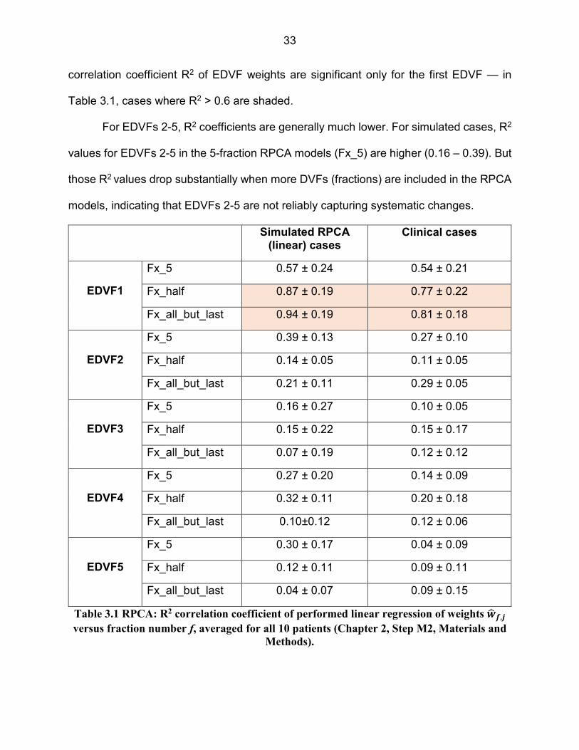
33

correlation coefficient R2 of EDVF weights are significant only for the first EDVF — in

Table 3.1, cases where R2 > 0.6 are shaded.

For EDVFs 2-5, R2 coefficients are generally much lower. For simulated cases, R2

values for EDVFs 2-5 in the 5-fraction RPCA models (Fx_5) are higher (0.16 – 0.39). But

those R2 values drop substantially when more DVFs (fractions) are included in the RPCA

models, indicating that EDVFs 2-5 are not reliably capturing systematic changes.

Simulated RPCA (linear) cases

Clinical cases

EDVF1

Fx_5 0.57 ± 0.24 0.54 ± 0.21

Fx_half 0.87 ± 0.19 0.77 ± 0.22

Fx_all_but_last 0.94 ± 0.19 0.81 ± 0.18

EDVF2

Fx_5 0.39 ± 0.13 0.27 ± 0.10

Fx_half 0.14 ± 0.05 0.11 ± 0.05

Fx_all_but_last 0.21 ± 0.11 0.29 ± 0.05

EDVF3

Fx_5 0.16 ± 0.27 0.10 ± 0.05

Fx_half 0.15 ± 0.22 0.15 ± 0.17

Fx_all_but_last 0.07 ± 0.19 0.12 ± 0.12

EDVF4

Fx_5 0.27 ± 0.20 0.14 ± 0.09

Fx_half 0.32 ± 0.11 0.20 ± 0.18

Fx_all_but_last 0.10±0.12 0.12 ± 0.06

EDVF5

Fx_5 0.30 ± 0.17 0.04 ± 0.09

Fx_half 0.12 ± 0.11 0.09 ± 0.11

Fx_all_but_last 0.04 ± 0.07 0.09 ± 0.15

Table 3.1 RPCA: R2 correlation coefficient of performed linear regression of weights c� d,e versus fraction number f, averaged for all 10 patients (Chapter 2, Step M2, Materials and

Methods).

34

The estimated anatomy epCT at the time of simulation was reconstructed by

applying O R (equation 2.4) to the wCT image. Figures 3.1 and 3.2 show result for the

same patients as for SPCA model. Figure 3.1 shows results for the patient D, for whom

RPCA gave the best results (out of the 10 patients studied). Figure 3.2 shows results for

patient A, for whom RPCA gave the worst results. In each case, top panels show pCT

(red) overlaid on the epCT (green). The left-most panel (A) is for a RPCA model

constructed from the first 5 treatment fractions. The middle panel (B) is for a RPCA model

constructed from the first 18 treatment fractions. The right-most panel (C) is for a RPCA

model constructed from all but the last treatment fraction. Lower panels in Figures 3.1

and 3.2 show the projections of all 35 simulated DVFs onto the leading EDVF. The error

bars represent ± one standard deviation of EDVF weight values across simulated

treatment courses having different random motion components. To generate these

results, 10 different treatment courses were simulated for each patient.

Figure 3.1 RPCA: Results of RPCA models generated from synthetic DVFs for patient D, for

whom PCA modeling gave the best results

35

Quantitative Evaluation

Figure 3.3 plots mean lengths of the image error vectors,‖pCT − epCT‖, equations

(2.6) and (2.7), as a function of the number of fractions F from which the RPCA model is

generated: Patient A, RPCA model generated from clinical CBCTs and DVFs; patient D,

RPCA model generated from clinical CBCTs and DVFs; patient A, RPCA model

generated from synthetic wCT and DVFs; patient D, RPCA model generated from

synthetic wCT and DVFs.

Although plotted against F = 5, 18, 34, clinical RPCA models utilized the first 5

CBCTs, approximately half of available CBCTs, and all but the final CBCT. Vector lengths

are scaled by 1/√ and plotted points are shifted slightly horizontally to avoid overlap of

Figure 3.2 RPCA: Results of RPCA models generated from synthetic DVFs for patient A, for

whom PCA modeling gave the worst results

36

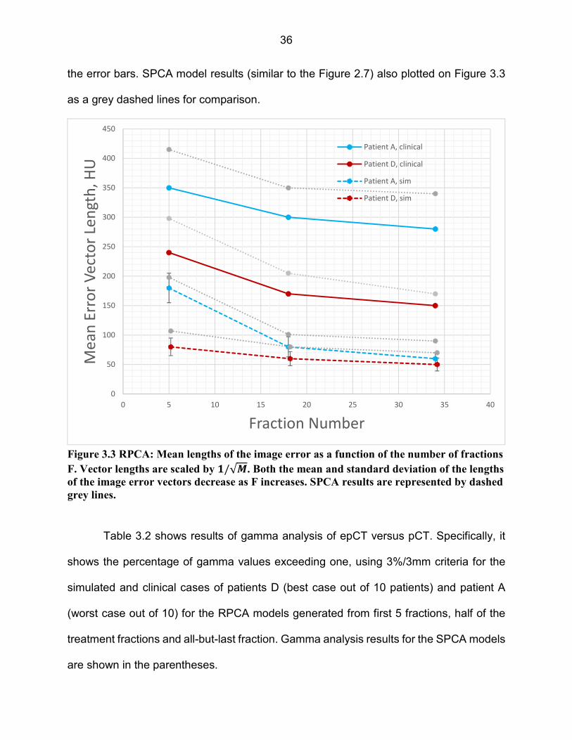
the error bars. SPCA model results (similar to the Figure 2.7) also plotted on Figure 3.3

as a grey dashed lines for comparison.

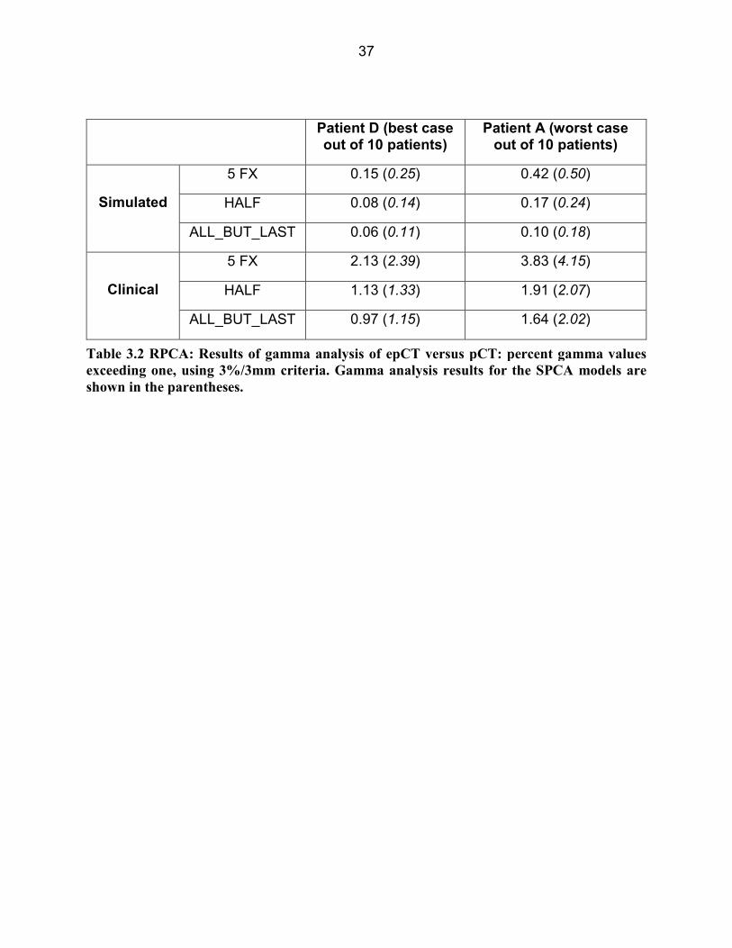
Table 3.2 shows results of gamma analysis of epCT versus pCT. Specifically, it

shows the percentage of gamma values exceeding one, using 3%/3mm criteria for the

simulated and clinical cases of patients D (best case out of 10 patients) and patient A

(worst case out of 10) for the RPCA models generated from first 5 fractions, half of the

treatment fractions and all-but-last fraction. Gamma analysis results for the SPCA models

are shown in the parentheses.

Figure 3.3 RPCA: Mean lengths of the image error as a function of the number of fractions

F. Vector lengths are scaled by f/√g. Both the mean and standard deviation of the lengths

of the image error vectors decrease as F increases. SPCA results are represented by dashed

grey lines.

0

50

100

150

200

250

300

350

400

450

0 5 10 15 20 25 30 35 40

Me

an

Err

or

Ve

cto

r Le

ng

th,

HU

Fraction Number

Patient A, clinical

Patient D, clinical

Patient A, sim

Patient D, sim

37

Patient D (best case out of 10 patients)

Patient A (worst case out of 10 patients)

Simulated

5 FX 0.15 (0.25) 0.42 (0.50)

HALF 0.08 (0.14) 0.17 (0.24)

ALL_BUT_LAST 0.06 (0.11) 0.10 (0.18)

Clinical

5 FX 2.13 (2.39) 3.83 (4.15)

HALF 1.13 (1.33) 1.91 (2.07)

ALL_BUT_LAST 0.97 (1.15) 1.64 (2.02)

Table 3.2 RPCA: Results of gamma analysis of epCT versus pCT: percent gamma values

exceeding one, using 3%/3mm criteria. Gamma analysis results for the SPCA models are

shown in the parentheses.

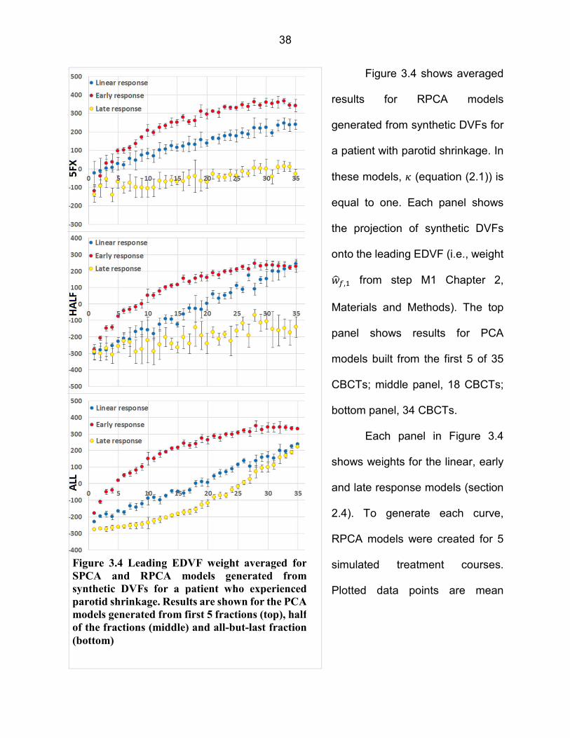
38

Figure 3.4 shows averaged

results for RPCA models

generated from synthetic DVFs for

a patient with parotid shrinkage. In

these models, * (equation (2.1)) is

equal to one. Each panel shows

the projection of synthetic DVFs

onto the leading EDVF (i.e., weight

���,� from step M1 Chapter 2,

Materials and Methods). The top

panel shows results for PCA

models built from the first 5 of 35

CBCTs; middle panel, 18 CBCTs;

bottom panel, 34 CBCTs.

Each panel in Figure 3.4

shows weights for the linear, early

and late response models (section

2.4). To generate each curve,

RPCA models were created for 5

simulated treatment courses.

Plotted data points are mean

Figure 3.4 Leading EDVF weight averaged for

SPCA and RPCA models generated from

synthetic DVFs for a patient who experienced

parotid shrinkage. Results are shown for the PCA

models generated from first 5 fractions (top), half

of the fractions (middle) and all-but-last fraction

(bottom)

39

weights. The error bars represent ± one standard deviation around the mean.

Figure 3.5 RPCA: 1st and 2nd EDVF weights for RPCA models generated from synthetic

DVFs for a patient who experienced parotid shrinkage. A linear response model was

assumed (Chapter 2, Materials and Methods), and r = s in equation 2.1, ensuring that

DVFs incorporated approximately 5 times the level of random motion seen in clinical

CBCTs

40

Figure 3.5 shows results for RPCA models generated from synthetic DVFs for a

patient who experienced parotid shrinkage. Left and right columns show the projections

of synthetic DVFs onto the two leading EDVFs. A linear response model was assumed

and * was equal to 5, ensuring that the magnitude of fraction-to-fraction random motion

was exaggerated to approximately 5 times the level seen in clinical CBCTs, making it

more difficult for PCA to extract systematic change from the random background.

As in Figure 3.4, plotted points on Figure 3.5 are the means of 5 simulated courses,

and error bars represent ± one standard deviation. Orange points show the EDVF weights

for the first F fractions, synthetic DVFs for which were included in the RPCA model (first

5, half and all-but-last). Blue points show weights for fractions F+1,..., N, synthetic DVFs

for which were excluded from the RPCA model. The orange line is the regression line for

orange points. The blue line is the regression line for all points, orange and blue. Orange

regression lines match the intercept M and slope N in equation 2.4. No blue linear

regression line is shown for the RPCA model generated from all-but-last fraction.

Figure 3.6 shows results for the RPCA models generated from clinical DVFs for a

patient who experienced weight loss in the left neck. In this case, plotted points are

projections of the clinical DVFs onto the first three EDVFs. Higher EDVFs (4+) were

omitted since they accounted for <10% of the total variation. Since clinical data is being

used, there is only one treatment course, and no error bars are plotted. Orange and blue

points and lines are as in Figure 3.5.

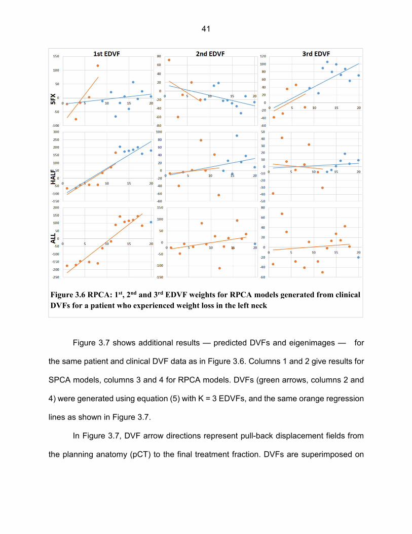
41

Figure 3.7 shows additional results — predicted DVFs and eigenimages — for

the same patient and clinical DVF data as in Figure 3.6. Columns 1 and 2 give results for

SPCA models, columns 3 and 4 for RPCA models. DVFs (green arrows, columns 2 and

4) were generated using equation (5) with K = 3 EDVFs, and the same orange regression

lines as shown in Figure 3.7.

In Figure 3.7, DVF arrow directions represent pull-back displacement fields from

the planning anatomy (pCT) to the final treatment fraction. DVFs are superimposed on

Figure 3.6 RPCA: 1st, 2nd and 3rd EDVF weights for RPCA models generated from clinical

DVFs for a patient who experienced weight loss in the left neck

42

the pCT image set to facilitate visual evaluation. Figure 3.7 shows DVFs for the same

axial slice through the patient anatomy.

Standard PCA

Figure 3.7 RPCA: Predicted DVFs and corresponding eigenimages (heat map

representation of DVF vector magnitudes) for the same patient as in Figure 3.7. DVF

arrow directions represent pull-back displacement fields from the planning anatomy

(pCT) to the final treatment fraction. The magnitude of displacements is at the same scale

as the background image.

43

The eigenimages in columns 1 and 3 of Figure 3.7 are heat-map representations

of the DVFs’ vector magnitude. Colors range from white (large magnitude displacements)

to red (intermediate magnitude displacements) to black (small or zero displacements).

The eigenimages are for the same axial slice as the DVFs.

Figure 3.8 shows the results similar to that shown on Figure 3.7, but for the patient

with parotid shrinkage and weight loss as a major anatomical change during radiotherapy.

Figure 3.8 RPCA: Predicted DVFs and corresponding eigenimages (heat map

representation of DVF vector magnitudes) for the patient with parotid shrinkage and

weight loss as a major anatomical change during radiation therapy.

44

Discussion

Qualitative Evaluation

Table 3.1 shows that R2 coefficients for the simulated linear cases for the first

EDVF have values close to 1, while EDVFs 2-5 produce much lower R2 values. This result

shows that the leading first EDVF can capture the simulated linear major mode of

anatomical change, while succeeding EDVFs capture residual errors and noise.

Figure 3.1 shows that RPCA modeling is capable of extracting the major mode of

anatomical change during head and neck radiation therapy. The leading EDVF

coefficients show a smooth progression during treatment, and the more CBCTs that are

included in the PCA model, the better the model becomes. This is indicated by a

progressive tightening of the standard deviations of EDVF weights as one moves from

model A (5 fractions), to model B (18 fractions), to model C (34 fractions).

In Figure 3.1 the modeled anatomical change, left neck lymph node shrinkage, is

large — it affects a relatively large volume of the patient’s anatomy. RPCA searches for

EDVFs that can explain variability across CBCT images. The modeled anatomical change

is large, and, similar to SPCA, the RPCA technique is easily able to ‘extract’ the major

deformation mode(s) from noisy data.

In Figure 3.2 (patient A, worst case for SPCA model), the modeled anatomical

change, bilateral parotid shrinkage, is relatively small — it affects a localized volume

around the parotids. In this case, as with the case on Figure 3.1, RPCA also successfully

isolates systematic anatomical change from other random variations. This is the opposite

of the SPCA modeling results, which had more difficulty in isolating the anatomical

45

change from other random variations that are present in the CBCT images. The RPCA

model is successful for patient D. The RPCA models for F=5 fraction show a fairly weak

linear progression of the leading EDVF coefficient, and the standard deviation of the

coefficients is large, indicating that the RPCA technique is having a difficult time ‘locking

onto’ the major deformation mode. But for the case F=18 and 35 the RPCA model become

good enough to predict the anatomy, with a higher level of confidence.

One of the conclusions of this study is that RPCA could successfully extract

smaller systematic anatomical changes from daily CBCT images.

Quantitative Evaluation

Figure 3.3 shows that larger HU errors occur for the RPCA models generated from

clinical CBCTs (lines (a) and (b)), than those generated from synthetic images and DVFs

(lines (c) and (d)). Comparing to SPCA, RPCA is more successful in extracting useful

models from synthetic cases and clinical CBCT images.

This conclusion is reinforced by the gamma results in Table 3.2. Those results

show that the number of voxels in epCT that disagree with pCT by more than 3% or 3

mm is fairly modest for the RPCA models generated from synthetic DVFs, but much larger

in models generated from clinical CBCTs. And in all cases RPCA models have a smaller

number of voxels which fail the 3% and 3mm gamma criteria than the SPCA models.

As for the SPCA models, quantitative results shown in Figure 3.3 and Table 3.2

may be used as an indirect way of testing the accuracy of DVFs, or the accuracy of the

reconstructed epCT versus the pCT image. Results of the quantitative analysis give an

idea of how the number of fractions used to build a model and random changes presented

46

in simulated and clinical data affect the quality of the last-fraction DVF and overall

accuracy of the epCT with respect to the pCT image.

PCA Performance

Figure 3.4 illustrates SPCA and RPCA performance under favorable conditions.

Figure 3.4 results are for a synthetic DVF set, where by design only one type of systematic

change is present in the patient data, and the magnitude of random changes is

comparable to clinical CBCTs. As a consequence, the error bars in Figure 3.4 are

relatively small, indicating consistent results across multiple simulated treatment courses.

Under these conditions, the bottom panel in Figure 3.4 shows that PCA can successfully

extract systematic motion using the leading EDVF. In the bottom panel, the curves for

early, linear and late response models mirror the profiles in Figure 2.3 (Chapter 2), as

one might hope. Figure 3.4 confirms that under favorable conditions — i.e., given

sufficient patient data to enable extraction of mean trends in the presence of random

background — PCA modeling can accurately extract the time-profile of anatomical

change.

For all response models, SPCA and RPCA perform well when able to build a model

from 34 fractions (Figure 3.4 bottom panel). When it is limited to half of the fractions

(middle panel), or the first 5 fractions (top panel), PCA continues to perform well for the

early and linear response models — the red and blue curves in the top 2 panels mirror

those in the bottom panel. However, it fails for the late response model in that the profile

of the late response weights in Figure 3.4, top and middle panels, does not mirror the late

response model of anatomical changes as shown in Figure 2.3. This illustrates an

47

intuitively obvious fact. PCA can only be successful if it is given sufficient motion data

from which to build a model. In the late response model, there is simply not enough

information present in early fractions for PCA to build a valid model.

The ability of SPCA and RPCA to generate patient-specific models from initial

treatment fractions for late-responding patients will depend on factors such as the size of

anatomical change relative to random motion, and will likely need to be evaluated on a

treatment site-by-site basis. A possible alternative is to develop population-based PCA

models of anatomical change, and use these as a starting point for all patients. Each

patient’s motion model could then be refined as patient-specific data is acquired over the

course of treatment. This work considers only patient-specific SPCA and RPCA models,

generated from a single patient’s data. Population based models represent a direction for

future research, and are not considered here. However, one might hope that population-

based models, based on large volumes of clinical data, could approach the PCA results

shown in the bottom panel of Figure 3.4.

Figure 3.5 illustrates (only) RPCA performance under challenging conditions.

Figure 3.5 results are for a synthetic DVF set, where by design only one type of systematic

change is present in the patient data, but where the magnitude of random changes is

exaggerated with respect to clinical CBCTs. As a consequence, the error bars Figure 3.5

are large, indicating a high degree of variability in DVFs across simulated treatment

courses. Under these conditions, the bottom two rows of Figure 3.5 show that RPCA is

still able to successfully extract systematic change when it has access to 18 of 35, or 34

of 35, fractions. Note that the regression lines in row 2 agree with those in row 3,

suggesting that RPCA is consistently identifying the same mode of motion in each EDVF.

48

What is new in this scenario is that RPCA now captures motion in more than one leading

EDVF. Figure 3.5 column 2 shows that the 2nd EDVF weight has non-zero slope,

indicating that it plays a role in modeling motion. For realistic motion scenarios, it is

expected that PCA will require more than one EDVF in order to faithfully model anatomical

motion.

The top row of Figure 3.5 shows that RPCA breaks down when it only has 5

fractions of data. In this scenario, the orange regression lines based on the first 5 fractions

do not match the blue regression lines based on 34 fractions. The blue lines agree with

lower plots, and so can be assumed to represent the ‘true’ EDVF weights. Predicted DVFs

based on the orange regression lines would be wildly inaccurate for later fractions, and

so produce erroneous predictions of anatomical change, cumulative radiation dose, etc.

This reinforces the conclusion that patient-specific PCA models may have limited utility

when based on a small number of initial fractions. As noted above, it may be desirable to

investigate population-based models to address this limitation.

Figure 3.5 shows results only for a linear response model. The size of error bars

in Figure 3.5 will make it difficult to reliably predict non-linear trends. One could fit different

non-linear curves to patient-specific EDVF coefficients, but the confidence intervals

around the fits may be large. If, however, one were to generate population PCA models

based on large volumes of H&N patient data, one could reasonably hope that average

trends could be extracted. Use of regularized PCA to generate population models remains

a subject for future research.

Figure 3.6 illustrates PCA performance for a clinical case, where the motion that is

present in the H&N CBCT image set is not known a priori. Figure 3.6 results are

49

qualitatively similar to those in Figure 3.5. They exhibit similar levels of noise (scatter of

plotted points around the trend lines) as seen in Figure 3.5. As in Figure 3.5, the orange

and blue trend lines in the lower two rows of Figure 3.6 are in good agreement, suggesting

that RPCA is consistently identifying the same mode of motion in each EDVF. The orange

trend lines in row 2 are in reasonable agreement with the blue lines in rows 2 and 3,

showing that an RPCA model based on 18 of 35 fractions can accurately predict EDVF

weight trends for remaining fractions. Note that the trend line associated with each EDVF

can reasonably be interpreted as systematic anatomical change, while the scatter of

points around the trend line represents the superimposed effect of random fraction-to-

fraction motion. The consistent trend lines in rows 2 and 3 show that RPCA is consistently

identifying the systematic component of anatomical change.

The top row of Figure 3.6 shows that PCA performs poorly when the model is

based on only the first 5 fractions. The orange trend lines do not agree with the blue trend

lines for EDVFs 1 and 2. This conclusion is consistent with the results for simulated DVFs

in Figures 3.4 and 3.5: patient-specific PCA models may have limited utility when based

on a small number of initial fractions.

In practice, weights on Figure 3.6, acquired from the projection of the clinical DVFs

onto the calculated EDVFs, are used to build a patient-specific RPCA model using

equation 2.4. For the RPCA models generated from the first F fractions (e.g., first 5

fractions, half of the fractions, or all-but-last fraction), subsequent weights of the F+1,…,

N fractions are calculated using a linear fit, and these weights are then used in equation

2.4 to model future fractions DVFs and corresponding anatomy.

50

Figures 3.7 and 3.8 provide a visual comparison of the SPCA and RPCA models

which were used to calculate the last fraction DVFs from the first 5, half, and all-but-last

fraction, and visual confirmation that RPCA is better than SPCA at identifying the

systematic component of H&N anatomical change. For reasons discussed below, SPCA

tends to produce noisy EDVFs, which are difficult to relate to clinically observable

changes. In Figures 3.7 and 3.8, SPCA EDVFs are non-zero across the whole patient

anatomy, even though dominant change is clearly confined to the left neck. In contrast,

at least when RPCA models are based on 18+ fractions, RPCA is successful at isolating

the dominant mode of change to the left neck area. RPCA’s ability to identify and

reproduce clinically observed change creates the potential to use RPCA to anticipate and

trigger adaptive re-planning decisions, and for quantitative treatment response

assessment.

Prior Applications of PCA

The idea of using PCA in radiotherapy is not novel. For example, the PCA

techniques were used to model patient-specific inter-fractional organ deformations in

prostate/rectum/bladder45. The results of that work showed that geometric variability is

governed by only the first few patient-specific eigenmodes, and using first 4 eigenmodes

to model organ deformations reduces residual errors to ≤2 mm. The results were later

used to assess the dosimetric detrimental effects that inter-fractional organ deformations

can have on a planned dose distribution47. Coverage-based treatment planning

techniques for prostate cases were also proposed based on the PCA organ deformation

model62. Furthermore, a population-based PCA model was developed and applied to

51

prostate cases40, showing that using the first 7 eigenmodes for patients in a database,

and first 15 eigenmodes for patients not in a database, reduces residual errors to ≤1 mm.

The main difference between this research and those described above is that this

work is focused on separating systematic changes in patients’ anatomy from random

changes. While this may not be necessary for the prostate/bladder/rectum cases, since

these areas don’t experience major systematic change during the radiotherapy, this

separation is important for H&N cases, since the anatomy could change significantly

during the treatment course.

The PCA model in H&N patients was also described and performed to create an

organ sample generator (OSG) for expected treatment dose construction63. The OSG

generated random samples of organs of interest during the treatment course to evaluate

dosimetric effects of the organ variations/deformations. The accuracy of the OSG

improved with the number of treatment fractions used for the PCA model, showing

discrepancy of the dose estimation within 1% for most organs after the first 3 weeks of

treatment. The OSG is a useful tool for dose accumulation estimation during the

treatment, but since it’s not trying to separate systematic changes in anatomy from

random changes, it could not be used in the prediction of the end-of-treatment anatomy.

Potential for Regularized PCA

ART promises to improve the quality of treatment received by radiation therapy

patients. However, adoption of ART has been held back by some practical considerations.

Repeatedly re-planning patient treatments can be costly, in terms of physician and

dosimetrist time and physics resources to check and QA treatment plans. There is

52

consequently a need for measurement-based models of anatomical change and

treatment response that would allow physicians to make educated decisions about when

to re-plan, which patients will benefit, etc.

RPCA has the potential to solve some of these challenges. RPCA is designed to

extract major modes of deformation from noisy imaging data, in principle allowing one to

discriminate real changes in the anatomy from background noise. If successful, RPCA

could be used to predict the future anatomy, and make re-planning decisions based on

dosimetric impact to the tumor and normal tissues.

SPCA is a well-known tool to find the major modes of variations in real-world

datasets. However, it was developed for datasets where the dimension of the problem is

less than the number of available data samples. In the present problem, the dimension of

the problem is 3M (i.e., 3 times the number of DVF voxels), which is on the order of 104-

105 for H&N voxel grids, and therefore much larger than the number of available CBCTs.

In this scenario SPCA models are extremely under-determined. As a result, SPCA has

a tendency to produce EDVFs than are noisy, and difficult to relate to clinically observable

anatomical changes.

RPCA addresses the problem of under-determination by supplementing SPCA

with additional constraints on eigenvectors. In the present work, RPCA adds smoothness

and sparseness constraints to SPCA. This has the effect of forcing EDVFs to be smooth

(i.e., physically realistic) and sparse (i.e., confined to localized regions of anatomy where

change is detected). Together, these constraints have a tendency to concentrate detected

anatomical change into a smaller number of leading EDVFs, which in turn makes it easier

53

to relate the EDVFs to clinically observable response. The application of regularized PCA

to adaptive radiation therapy is a novel contribution of this work.

This work can be considered to fall within radiomics, which studies how to extract

quantitative information from the medical images in order to characterize treatment

response. In the present case, RPCA is being used to reduce high-dimensional imaging

data to a small number of anatomical motion modes. Detecting tumor deformation during

treatment will permit assessment of treatment response. Similarly, detecting the response

of normal tissues, such as parotid glands, may permit quantitative evaluation of

radiotherapy-related complications.

Study Limitations

Acquiring accurate DVFs between patient images is a key step in this study

because the results of PCA modeling are dependent on the quality of input DVFs.

Therefore, the choice of DIR algorithm and its registration parameters is one of the most

important factors for accurate modeling. In this study Pinnacle’s diffeomorphic demons

algorithm58 was used for deformable registrations. Although we visually verified the

registration results, use of a different algorithm may produce slightly different results from

those presented in this study. In this work other DIR algorithms were not used apart from

those implemented in Pinnacle®, since all the codes for DVFs manipulations were

implemented considering Pinnacle’s® DVF internal structure and performed using

Pinnacle® plugin functionality. One of our intended future works is to use different

commercial and open-source DIR algorithms to understand the effects on the resultant

PCA models.

54

Quantification of DIR/DVF accuracy is a major challenge for adaptive radiation

therapy, on which much research is being expended. It is outside the scope of this work

to attempt to quantify the accuracy of DIR algorithms. Instead, we expect that reliable DIR

algorithms will emerge from ongoing research and clinical use. Although DVF accuracy

will have an impact on the accuracy of PCA models, we note that regularized PCA may

be part of the answer to this issue. RPCA has the potential to extract smooth and

physically meaningful EDVFs from noisy CBCT data, including the noise introduced by

DVF uncertainties. One can reasonably hope that RPCA models will be insensitive to

small scale uncertainties present in DVFs, and instead extract larger scale anatomical

changes corresponding to observable clinical change.

One other important study limitation is the CF used to acquire DVFs. In this study,

CF of 7 was used, which reduces the precision of acquired DVFs compared to non-

compressed DVFs. This, in turn, reduces the precision of the motion model and could

underestimate the effects of anatomical motion presented in the patient. This effect can

be seen in Figures 3.1 and 3.2 – on the left neck lymph node shrinkage (Figure 3.1) and

parotid shrinkage (Figure 3.2). RPCA does not precisely capture these anatomical

changes due to the large CF used, and epCT is not completely matched to the pCT image,

even though it still shows better performance than SPCA, giving an advantage of better

smoothness and sparseness due to the regularized approach.

The regularized approach in PCA requires a calculation of penalty matrix of very

large size, ~ (3M) 2, which puts very high requirements on computational resources. In

this work, CF of 7 was used, and random-access memory (RAM) of ~ 100-120 GB

(depending on the patient) was required, and calculation time was ~ 7 days on the Wayne

55

State University High Performance Computing Grid. The calculation time potentially could

be improved by using a parallel computing – dividing the calculation of the penalty matrix

for RPCA models between multiple processes.

Conclusion

For H&N patients treated with external beam radiation therapy, a PCA model (both

standard and regularized) is a potential tool to identify patient anatomy changes early in

the treatment course, and use these to make educated adaptive re-planning decisions.

This study used synthetic (but realistic) DVFs, as well as clinical CBCTs, to evaluate the

ability of the PCA method to extract useful models of anatomical change. In particular, a

primary goal of this work was to evaluate the ability of PCA to separate systematic from

random changes present in CBCT images.

The study shows that both SPCA and RPCA can capture the major mode of

systematic anatomical deformation in the leading EDVF. However, the SPCA approach

is most successful at identifying large changes (e.g., significant lymph node shrinkage),

and less successful at identifying small changes (e.g., smaller changes in parotid glands).

SPCA is challenged by the variety of deformations and noise in clinical CBCT images,

and therefore fails to extract major modes of systematic change that are known to be

present. Conversely, the RPCA approach is able to identify smaller systematic changes

in the presence of the random fraction-to-fraction changes. The current drawback of the

RPCA approach is the time of the calculation and memory requirements.

56

CHAPTER 4 “DOSIMETRIC ASSESSMENT OF EFFECTS OF SYSTEMATIC AND RANDOM FRACTION-TO-FRACTION ANATOMICAL CHANGES IN HEAD AND

NECK PATIENTS”

Introduction

Decisions about whether to perform ART for a specific H&N patient could be made

by the physician by either comparing the patient’s daily anatomical images (like CBCT)

with the pCT image and deciding if anatomical changes are large enough to significantly

alter the planned dose distribution, or by evaluating the mask used for patient

immobilization and positioning, or using other subjective indicators, such as the

physician’s experience in such cases. Currently, there are no clear quantitative indicators

regarding whether or not perform ART for a specific patient64.

Using advanced treatment techniques like IGRT, one of the potential quantitative

indicators for ART in H&N patients could be the measuring of the actual dose delivered

to date to targets and OARs, which could be done by calculating “dose of the day” onto

re-sampled CT images using DIR and then accumulating it back onto the pCT65. Such

“dose of the day” calculations, which would give accumulated dose up to but not beyond

the current fraction, can be used in the clinic for tracking the dose delivered to the patient

in each fraction and comparing it with the planned dose distributions. The drawback of

this method is that it is retrospective: one can react to OAR overdoses or target

underdoses once they have happened, but there is no good basis for anticipating them

and correcting them in advance, while one still has maximum flexibility to re-plan and

correct the dose distribution.

In this work one of the potential solutions to this problem is presented. Using

developed motion models based on RPCA approach (Chapter 3), not only “dose of the

57

day” is calculated and accumulated, but also dose of the future fractions is calculated on

re-sampled “future CT” images. The predicted cumulative dose is then compared to the

planned dose, enabling re-planning decisions to be made earlier in the treatment course.

Additionally, at the end of the course, the predicted cumulative dose can be compared

with the true cumulative dose, to evaluate the accuracy of the RPCA-based dose

predictions.

There are two main hypotheses in this study:

H1: RPCA models can quantify deviations between planned and delivered

cumulative dose caused by systematic anatomical changes.

H2: RPCA models can quantify deviations between planned and delivered

cumulative dose caused by both systematic and random anatomical changes.

This study provides a testing framework to evaluate the accuracy of RPCA-based

anatomical models at predicting cumulative dose. Within this framework it is instructive to

separately calculate the dosimetric effects of systematic versus random changes. In this

way one can assess the relative contributions of systematic versus random changes. One

can then make reliable re-planning decisions based on detected systematic changes, and

determine PTV margins to absorb residual random changes.

Materials and Methods

Two H&N patients from the dataset described in Chapter 2, who experienced large

systematic changes during the course of radiation therapy, were chosen in order to

conduct a dosimetric study. The first of the selected patients experienced parotid

shrinkage, and was treated with 70Gy in 33 fractions. The second selected patient

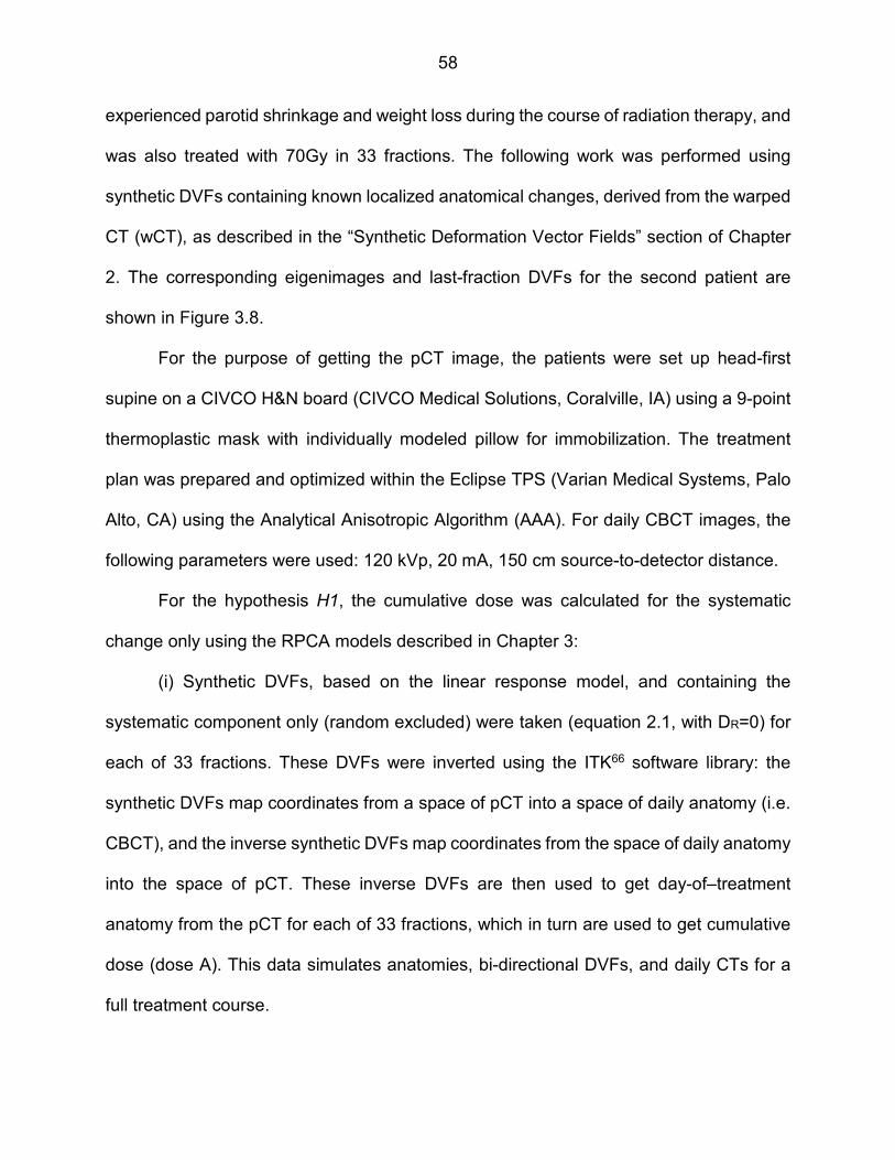
58

experienced parotid shrinkage and weight loss during the course of radiation therapy, and

was also treated with 70Gy in 33 fractions. The following work was performed using

synthetic DVFs containing known localized anatomical changes, derived from the warped

CT (wCT), as described in the “Synthetic Deformation Vector Fields” section of Chapter

2. The corresponding eigenimages and last-fraction DVFs for the second patient are

shown in Figure 3.8.

For the purpose of getting the pCT image, the patients were set up head-first

supine on a CIVCO H&N board (CIVCO Medical Solutions, Coralville, IA) using a 9-point

thermoplastic mask with individually modeled pillow for immobilization. The treatment

plan was prepared and optimized within the Eclipse TPS (Varian Medical Systems, Palo

Alto, CA) using the Analytical Anisotropic Algorithm (AAA). For daily CBCT images, the

following parameters were used: 120 kVp, 20 mA, 150 cm source-to-detector distance.

For the hypothesis H1, the cumulative dose was calculated for the systematic

change only using the RPCA models described in Chapter 3:

(i) Synthetic DVFs, based on the linear response model, and containing the

systematic component only (random excluded) were taken (equation 2.1, with DR=0) for

each of 33 fractions. These DVFs were inverted using the ITK66 software library: the

synthetic DVFs map coordinates from a space of pCT into a space of daily anatomy (i.e.

CBCT), and the inverse synthetic DVFs map coordinates from the space of daily anatomy

into the space of pCT. These inverse DVFs are then used to get day-of–treatment

anatomy from the pCT for each of 33 fractions, which in turn are used to get cumulative

dose (dose A). This data simulates anatomies, bi-directional DVFs, and daily CTs for a

full treatment course.

59

(ii) Using the RPCA model (Chapter 3, Materials and Methods) and synthetic DVFs

from step (i), predicted DVFs were calculated using first 5, half and all but last treatment

fractions. Inverse DVFs and predicted CT images for each of 33 fractions were acquired

and used to predict cumulative dose (dose B) at the final fraction.

(iii) The above procedure generates three dose distributions:

- Planned dose: This is the original planned dose distribution generated on

the planning CT

- Dose A: For a simulated treatment course, this is the “true” cumulative dose

at the end of the course, assuming zero random changes.

- Dose B: For a simulated treatment course, this is the dose predicted by an

RPCA model, where the model could be derived from the first 5, half, or all but last

simulated fractions, assuming zero random changes.

For relevant structures, Dose Volume Histograms (DVHs) for 3 scenarios were

compared: planned dose, dose A, and dose B. If H1 is correct, the expectation is to see

dose A similar to dose B. In this study “similarity” was checked by comparing the

maximum and the mean dose deviations between doses A and B which were expected

to be close enough to be clinically equivalent. We also expect that doses A and B can

differ significantly from the planned dose, depending on structure, due to the presence of

significant anatomical changes over the treatment course.

For hypothesis H2, the cumulative dose was calculated for both systematic and

random changes using the RPCA models:

(iv) Synthetic DVFs, based on the linear response model, and containing both

systematic component and 10 different simulations of random components were taken

60

(equation 2.1) for each of 33 fractions. Using the same procedure as in step (i), these

DVFs were inverted and then used to get cumulative dose in the presence of systematic

and random components (dose C).

(v) Using RPCA model and synthetic DVFs with simulated random components

from step (iv), predicted DVFs were calculated using first 5, half and all but last treatment

fractions, inverse DVFs and predicted CT images for each of 33 fractions were acquired

and used to get cumulative dose (dose D).

(vi) The above procedure generates three dose distributions:

- Planned dose: This is the original planned dose distribution generated on

the planning CT

- Dose C: For a simulated treatment course, this is the “true” cumulative dose

at the end of the course, assuming non-zero random changes.

- Dose D: For a simulated treatment course, this is the dose predicted by an

RPCA model, where the model could be derived from the first 5, half, or all but last

simulated fractions, assuming non-zero random changes.

In the same manner as above, for relevant structures, DVHs for 3 scenarios were

compared: planned dose, dose C, and dose D. If H2 is correct, the expectation is to see

dose C similar to dose D, and both of these different from the planned dose.

A CF of 7 was used for this study for the reasons discussed in Chapter 3 –

generation of RPCA models using our current method is numerically and memory

intensive, so it was necessary to adopt a CF of 7 in order to keep computing resources

and execution times within acceptable limits.

However, aggregation of DVF voxels has the effect of smoothing DVFs, reducing

61

their spatial resolution, at least in the XY-plane. As shown in Chapters 2 and 3 (Figures

2.5, 2.6, 3.1, 3.2), using large CF for the acquisition of the DVFs could underestimate the

anatomical motion in the patient even if it was captured correctly in the CBCTs.

To assess this effect, the predicted dose from RPCA models (where anatomical

motion could be underestimated due to DVF compression) was compared to the “real”

accumulated dose and to the planned dose. “Real” dose accumulation (dose R) was

performed in VelocityAI (version 3.2.0, Varian Medical Systems) using the method

described in Kumarasiri et al67. Acquiring dose R does not require DVFs compression,

and therefore it accounts for all anatomical motion, subject to the DIR precision and

uncertainty.

Dose R is then compared to planned dose, and doses A, B, C and D. If compressed

DVFs in fact underestimate the anatomical changes in the patient, dose R is expected to

be different from the planned dose, and the DVHs associated with doses A, B, C and D

are expected to be in between the DVH of the planned dose and DVH of the dose R.

The percent differences between the planned dose and simulated (dose A, C),

modeled (dose B, D), or accumulated dose (dose R) was calculated using the following

equation:

∆ = $uv�w/wxyz{/|}}~w�u�{|��zyu�{|��zy

' × 100 (4.1)

Results

Figures 4.1 and 4.2 show the DVHs for the left parotids of patients 1 and 2. On

these figures, planned DVH (blue) is compared to the calculated DVHs of patients 1 and

2 with the systematic only (Figure 4.1, dose A, green) and systematic and random

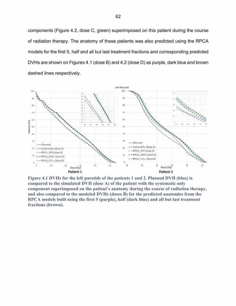
62

components (Figure 4.2, dose C, green) superimposed on this patient during the course

of radiation therapy. The anatomy of these patients was also predicted using the RPCA

models for the first 5, half and all but last treatment fractions and corresponding predicted

DVHs are shown on Figures 4.1 (dose B) and 4.2 (dose D) as purple, dark blue and brown

dashed lines respectively.

Figure 4.1 DVHs for the left parotids of the patients 1 and 2. Planned DVH (blue) is

compared to the simulated DVH (dose A) of the patient with the systematic only

component superimposed on the patient’s anatomy during the course of radiation therapy,

and also compared to the modeled DVHs (doses B) for the predicted anatomies from the

RPCA models built using the first 5 (purple), half (dark blue) and all but last treatment

fractions (brown).

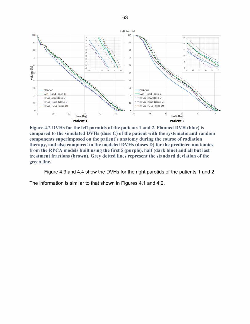
63

Figure 4.3 and 4.4 show the DVHs for the right parotids of the patients 1 and 2.

The information is similar to that shown in Figures 4.1 and 4.2.

Figure 4.2 DVHs for the left parotids of the patients 1 and 2. Planned DVH (blue) is

compared to the simulated DVHs (dose C) of the patient with the systematic and random

components superimposed on the patient’s anatomy during the course of radiation

therapy, and also compared to the modeled DVHs (doses D) for the predicted anatomies

from the RPCA models built using the first 5 (purple), half (dark blue) and all but last

treatment fractions (brown). Grey dotted lines represent the standard deviation of the

green line.

64

Figure 4.3 DVHs for the right parotids of the patients 1 and 2. Planned DVH (blue) is

compared to the simulated DVH (dose A) of the patient with the systematic only component

superimposed on the patient’s anatomy during the course of radiation therapy, and also

compared to the modeled DVHs (doses B) for the predicted anatomies from the RPCA

models built using the first 5 (purple), half (dark blue) and all but last treatment fractions

(brown).

Figure 4.4 DVHs for the right parotids of the patients 1 and 2. Planned DVH (blue) is

compared to the simulated DVHs (dose C) of the patient with the systematic and random

components superimposed on the patient’s anatomy during the course of radiation

therapy, and also compared to the modeled DVHs (doses D) for the predicted anatomies

from the RPCA models built using the first 5 (purple), half (dark blue) and all but last

treatment fractions (brown). Grey dotted lines represent the standard deviation of the

green line.

65

Figures 4.5 and 4.6 show the DVHs for the spinal cords of the patients 1 and 2.

The information is similar to that shown in Figures 4.1, 4.2, 4.3 and 4.4.

Figure 4.5 DVHs for the spinal cords of the patients 1 and 2. Planned DVH (blue) is

compared to the simulated DVH (dose A) of the patient with the systematic only component

superimposed on the patient’s anatomy during the course of radiation therapy, and also

compared to the modeled DVHs (doses B) for the predicted anatomies from the RPCA

models built using the first 5 (purple), half (dark blue) and all but last treatment fractions

(brown).

66

Figure 4.7 (A) shows the pCT image (red) overlaid on the resampled CBCT image

of the last treatment fraction for the patient 2 who experienced parotid shrinkage and

weight loss during the course of radiation therapy. The CBCT is resampled using the

diffeomorphic demons DVF compressed with a CF of 7. Figure 4.7 (B) shows the pCT

image (red) overlaid on the epCT (green) for this patient; the epCT image is acquired

using equation 2.4 from Chapter 2. Red arrows show the underestimation of the parotids

movement due to the large CF used for the DVFs. Figure 4.7 (C) shows the pCT image

(red) overlaid on the last fraction CBCT image.

Figure 4.6 DVHs for the spinal cords of the patients 1 and 2. Planned DVH (blue) is

compared to the simulated DVHs (dose C) of the patient with the systematic and random

components superimposed on the patient’s anatomy during the course of radiation

therapy, and also compared to the modeled DVHs (doses D) for the predicted anatomies

from the RPCA models built using the first 5 (purple), half (dark blue) and all but last

treatment fractions (brown). Grey dotted lines represent the standard deviation of the

green line.

67

Figures 4.8, 4.9 and 4.10 show the results of the movement underestimation of the

patients anatomy by the DVFs by comparing the planned (blue) and modeled (green and

brown) DVHs presented above with the “real” accumulated DVH (red) for the left and right

parotids, and spinal cord.

Figure 4.7 Patient 2: (A) pCT (red) overlaid on the resampled CBCT of the last treatment

fraction. CBCT is resampled using the diffeomorphic demons DVF compressed with the

factor 7; (B) pCT (red) overlaid on the epCT (green). Red arrows show the

underestimation of the parotids movement due to the large CF used for the DVFs; (C) pCT

(red) overlaid on the last fraction CBCT (green).

Figure 4.8 Patients 1 and 2: Comparison of the planned DVHs (blue) for the left parotid

glands vs. the simulated DVHs (green, brown) vs. “real” cumulative DVH.

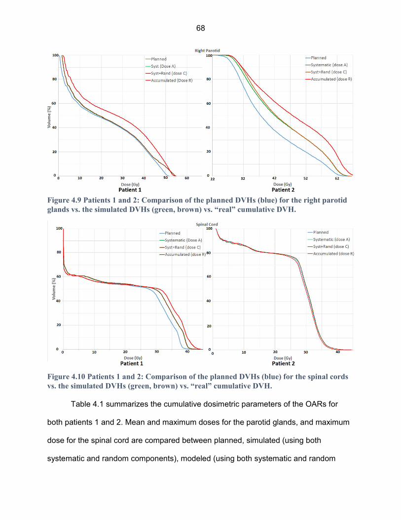
68

Table 4.1 summarizes the cumulative dosimetric parameters of the OARs for

both patients 1 and 2. Mean and maximum doses for the parotid glands, and maximum

dose for the spinal cord are compared between planned, simulated (using both

systematic and random components), modeled (using both systematic and random

Figure 4.9 Patients 1 and 2: Comparison of the planned DVHs (blue) for the right parotid

glands vs. the simulated DVHs (green, brown) vs. “real” cumulative DVH.

Figure 4.10 Patients 1 and 2: Comparison of the planned DVHs (blue) for the spinal cords

vs. the simulated DVHs (green, brown) vs. “real” cumulative DVH.

69

components) and cumulative cases. The relative difference from the planned dose

(equation 4.1) is presented in parentheses.

Patient 1 Patient 2

Dmean Dmax Dmean Dmax

Left

parotid

Planned 23.5 51.0 44.6 74.4

Simulated, dose C 25.1

(6.8%)

54.1

(6.1%)

49.8

(11.7%)

75.9

(2.0%)

Modeled,

dose D

5fx 23.7

(0.9%)

52.5

(2.9%)

46.6

(4.5%)

74.9

(0.7%)

Half 25.1

(6.8%)

53.9

(5.7%)

49.3

(10.5%)

75.6

(1.6%)

All 25.7

(9.4%)

54.3

(6.5%)

50.5

(13.2%)

75.7

(1.7%)

Cumulative 27.0

(14.9%)

55.9

(9.6%)

52.5

(17.7%)

76.6

(3.0%)

Right

Parotid

Planned 23.0 51.8 41.7 65.2

Simulated, dose C 24.5

(6.5%)

54.3

(4.8%)

47.9

(14.9%)

67.9

(4.1%)

Modeled,

dose D

5fx 23.5

(2.2%)

51.0

(-1.5%)

44.5

(6.7%)

66.3

(1.7%)

Half 24.9

(8.3%)

54.8

(5.8%)

47.1

(12.9%)

67.8

(4.0%)

All 24.4

(6.1%)

54.3

(4.8%)

48.6

(16.5%)

68.7

(5.4%)

Cumulative 25.7

(11.7%)

55.1

(6.4%)

50.1

(20.1%)

69.8

(7.1%)

Dmax Dmax

Spinal

Cord

Planned 42.1 45.2

Simulated, dose C 43.9 (4.3%) 45.2 (0%)

Modeled,

dose D

5fx 42.9 (1.9%) 44.9 (-0.7%)

Half 43.3 (2.9%) 45.3 (0.2%)

All 43.5 (3.3%) 45.3 (0.2%)

Cumulative 45.2 (7.4%) 45.4 (0.4%)

Table 4.1 Planned, simulated, modeled and accumulated dosimetric parameters for the

patients (in Gy). The relative percentage difference from the planned dose presented in

parentheses.

70

Discussion

Figures 4.1, 4.3 and 4.5 show the DVHs for the simulated and modeled left parotid,

right parotid and spinal cord respectively when only systematic changes are introduced

in patients 1 and 2 with parotid shrinkage, and parotid shrinkage and weight loss as a

major mode of anatomical change during radiation therapy, respectively. These are

compared to the planned DVH. It can be seen qualitatively that the planned dose to the

parotids is different from the simulated (Figures 4.1, 4.3, dose A) and modeled doses

(Figures 4.1, 4.3, dose B). Due to the shrinkage, the parotids are shifted into the area of

higher dose and accumulate more dose than was planned. However, changes in the

parotids did not affect the movement of the spinal cord of the patient 2 during the radiation

therapy course, and the dose to the spinal cord didn’t change for the simulated course

compared to the planning course. On the other hand, as shown in Table 4.1, patient 1

experienced dose escalation from the planned (42.1Gy) to simulated (45.2Gy) treatment

course. While in this case this unintended 3 Gy increase in the dose to a critical OAR

would likely be acceptable24, this is not always the case. For example, if the modeled

maximum dose to the spinal cord had been 55 Gy, additional dose in such case would

predict a substantial increase in Normal Tissue Complication Probability (NTCP).

For the patients 1 and 2, RPCA anatomy modeling when using DVFs from the first

5 fractions qualitatively showed larger deviation from the simulated treatment course for

the parotids, especially in the areas of higher doses (Figures 4.1, 4.3). RPCA models

when using DVFs from the half and all-but-last fraction show good conformity with the

simulated treatment course. This means that when using enough data for building the

model, RPCA can identify and capture the major mode of anatomical change and it can

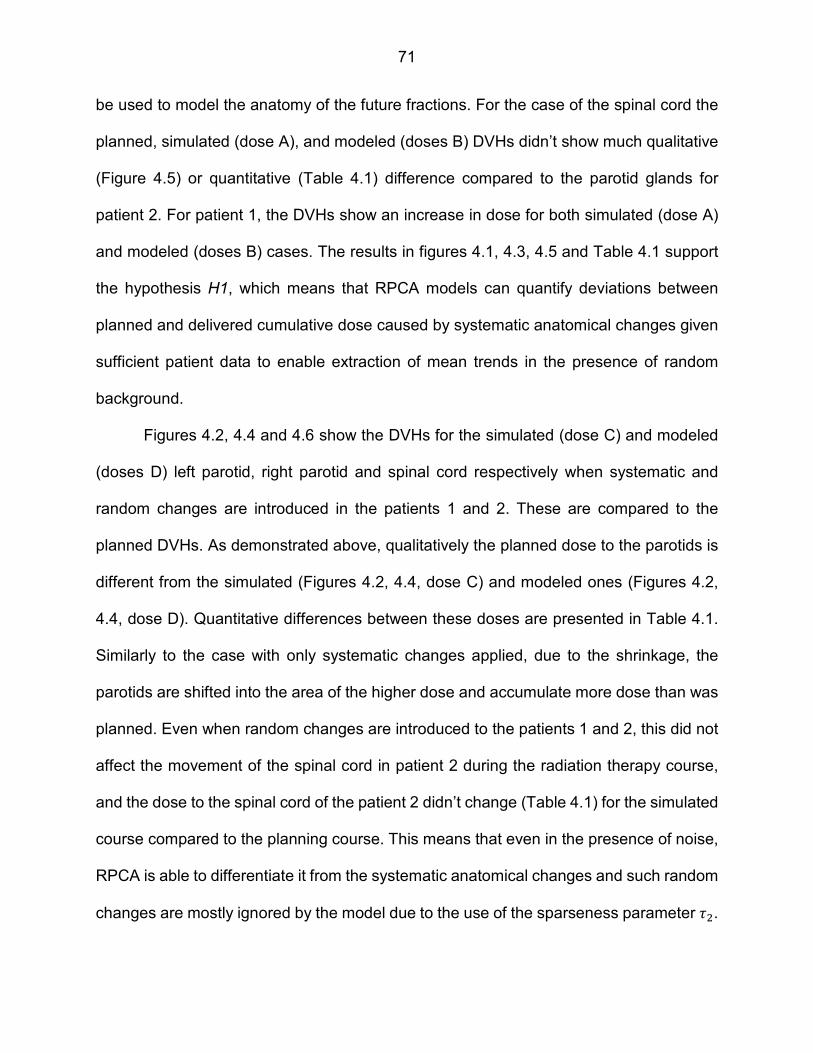
71

be used to model the anatomy of the future fractions. For the case of the spinal cord the

planned, simulated (dose A), and modeled (doses B) DVHs didn’t show much qualitative

(Figure 4.5) or quantitative (Table 4.1) difference compared to the parotid glands for

patient 2. For patient 1, the DVHs show an increase in dose for both simulated (dose A)

and modeled (doses B) cases. The results in figures 4.1, 4.3, 4.5 and Table 4.1 support

the hypothesis H1, which means that RPCA models can quantify deviations between

planned and delivered cumulative dose caused by systematic anatomical changes given

sufficient patient data to enable extraction of mean trends in the presence of random

background.

Figures 4.2, 4.4 and 4.6 show the DVHs for the simulated (dose C) and modeled

(doses D) left parotid, right parotid and spinal cord respectively when systematic and

random changes are introduced in the patients 1 and 2. These are compared to the

planned DVHs. As demonstrated above, qualitatively the planned dose to the parotids is

different from the simulated (Figures 4.2, 4.4, dose C) and modeled ones (Figures 4.2,

4.4, dose D). Quantitative differences between these doses are presented in Table 4.1.

Similarly to the case with only systematic changes applied, due to the shrinkage, the

parotids are shifted into the area of the higher dose and accumulate more dose than was

planned. Even when random changes are introduced to the patients 1 and 2, this did not

affect the movement of the spinal cord in patient 2 during the radiation therapy course,

and the dose to the spinal cord of the patient 2 didn’t change (Table 4.1) for the simulated

course compared to the planning course. This means that even in the presence of noise,

RPCA is able to differentiate it from the systematic anatomical changes and such random

changes are mostly ignored by the model due to the use of the sparseness parameter i(.

72

RPCA anatomy modeling when using DVFs from the first 5 fractions showed larger

deviation from the simulated treatment course for both parotids (Figures 4.2, 4.4, Table

4.1), especially in the areas of higher doses. But RPCA models built using DVFs from the

half and all-but-last fraction show good conformity with the simulated treatment course.

That also means that RPCA can identify and capture the major mode of anatomical

change even in the presence of the random changes and it can be used to model the

anatomy of the future fractions. For the spinal cord of the patient 1 (Figure 4.6), planned,

simulated (dose C) and modeled (doses D) showed the difference of up to 3.3% (Table

4.1) from the planned DVH. For the spinal cord of the patient 2 (Figure 4.6), planned,

simulated (dose C) and modeled (doses D) DVHs didn’t show much difference (<1%,

Table 4.1) from planned DVH compared to the parotid glands. The results in figures 4.2,

4.4 and 4.6 support the hypothesis H2, which means that RPCA models can quantify

deviations between planned and delivered cumulative dose caused by both systematic

and random anatomical changes.

The RPCA models in this work used DVFs acquired using a large CF value (7),

and using such compressed DVFs usually underestimates the anatomical changes

present in the patients. Figure 4.7 (A) shows the pCT image (red) overlaid on the

resampled CBCT image of the last treatment fraction. CBCT is resampled using the

diffeomorphic demons DVF compressed with a factor of 7. Figure 4.7 (B) shows the pCT

image (red) overlaid on the epCT (green) of the patient. Figure 4.7 (C) shows the pCT

image (red) overlaid on the last fraction CBCT image (green). Ideally, it is expected that

pCT and epCT images would be exactly the same, but as can be seen in Figure 4.7 (B),

motion of the parotids is underestimated by the model due to the large CF of the DVFs.

73

Such effects are not only seen on the epCT image acquired from the modeled DVFs, but

also on resampled last fraction CBCT image acquired using real clinical DVFs

compressed with the same CF, as seen on Figure 4.7 (A). This means that even though

RPCA could capture the correct major mode of anatomical changes in the patient from

compressed DVFs, it is possible that these changes would be underestimated and the

model will show less movement in the anatomy than in the real case. Another challenge

of using the compressed DVFs is that they can’t capture the movement on a “wiggly”

edge, like those on the parotids in Figure 4.7. So using a large CF will suppress the

smaller and “wigglier” anatomical changes in the DVFs, and therefore RPCA would not

be able to extract such changes form this dataset. In general, the quality of the RPCA

models is dependent on the quality of the input data, the DVFs.

Such underestimation of the anatomical changes could lead to the underestimation

of the dose distribution changes in the patient. This effect is shown for the parotids and

spinal cords of the patients 1 and 2 on Figures 4.8, 4.9 and 4.10. On these figures,

planned DVH (blue) is compared to the simulated DVH, acquired from the anatomy

resampled with the compressed DVFs (green, brown), and in turn compared to the “real”

accumulated DVH (red) for the patient. As can be seen, the “real” DVH is shifted to the

right with respect to the modeled DVHs. This means that underestimation of the parotid

shrinkage in the modeled cases leads to the underestimation of the dose received by

parotids due to their shift into the high dose region.

Based on the visual examination of the performance of the compressed DVFs

(Figure 4.7), and subsequent dosimetric DVHs’ deviations calculated based on these

corresponding DVFs (Table 4.1), future work on RPCA models requires use of DVFs with

74

smaller CF in order to capture smaller changes in the anatomy.

Conclusion

This work showed that RPCA has the potential to identify the major mode of

anatomical changes during the radiotherapy course in which allows the prediction of

dose for the course of treatment. There are some challenges presented with the DVFs

compressed using a large CF, so use of smaller CF should be considered for the future

work. There is a hope, that using RPCA modeling could provide a roadmap for how to

use PCA in ART: (i) RPCA models are generated based on initial fractions, (ii) dose

deviations due to underlying systematic change are projected for future fractions to

trigger re-planning decisions, (iii) effects of random changes are superimposed to guide

what margins should be used.

75

CHAPTER 5 “CONCLUSIONS AND FUTURE WORK”

Summary of Findings

As discussed in Chapter 1, the modeling of anatomical changes over the course

of head-and-neck treatment is essential to answer practical questions such as: What

anatomical changes are important? How do we measure them? When to trigger re-

planning? And how best to perform the re-planning? Such models should take into

account not only rigid body transformations but also deformations, and be capable of

extracting useful information about changes in patient anatomy, ideally early in the

radiation treatment course.

PCA was chosen as a core element of this work because of its use in developing

motion models of anatomical changes during the radiation therapy course. PCA has been

used in many previous applications, specifically in the field of radiation therapy47, 49-52.

However, the implementation of PCA models has not been utilized for extracting

systematic changes in patient anatomy during a H&N radiation therapy course.

Two approaches to the PCA were implemented: a standard approach to PCA

(SPCA, Chapter 2) and a more advanced regularized approach (RPCA, Chapter 3).

The results showed that for the H&N patients treated with external beam radiation

therapy included in this cohort, a SPCA model was a potential tool for identifying patient

anatomy changes early in the treatment course, and making educated adaptive re-

planning decisions. The study showed that under the right conditions, SPCA can capture

the major mode of systematic anatomical deformation in the leading EDVF. However,

SPCA is most successful at identify large changes (e.g., significant lymph node

76

shrinkage), and less successful at identifying small changes (e.g., smaller changes in

parotid glands). Additionally, SPCA is challenged by the variety of deformations and noise

in clinical CBCT images, and therefore fails to extract major modes of systematic change

that are known to be present.

In order to successfully model anatomical changes in clinical CBCT images, the

basic SPCA technique has been refined using a regularized approach to the PCA, RPCA

(Chapter 3). Using a regularized approach, we have shown that the RPCA model is a

potential tool for identifying patient anatomy changes early in the treatment course. In

contrast to SPCA, the RPCA approach was able to identify smaller changes compared to

the random fraction-to-fraction changes. The drawback of the RPCA approach is the time

necessary for the calculation, memory requirements and use of large CF for the DVFs.

The dosimetric study (Chapter 4) showed that PCA models have the potential to

identify the major mode of anatomical changes during the radiotherapy course which

allow the prediction of dose for the treatment course. There were some challenges

presented with the DVFs compressed using a large CF, so using smaller CF should be

considered in future work. In summary, the work presented provides direction for the

implementation of RPCA modeling in ART.

Future Work

One of the main directions of the current research going forward is the

accumulation of the H&N patient datasets in order to create population-based models of

anatomical changes. Population based models will be generated from large numbers of

patients, and should therefore capture modes of anatomical change that apply to most

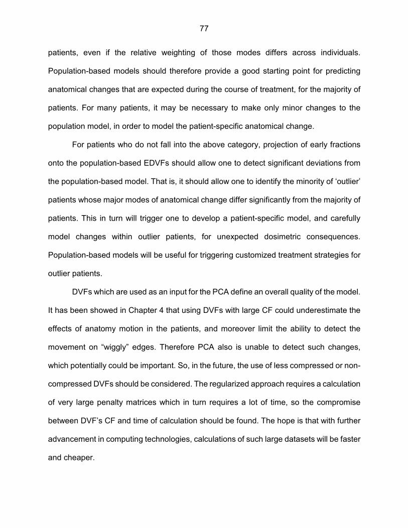
77

patients, even if the relative weighting of those modes differs across individuals.

Population-based models should therefore provide a good starting point for predicting

anatomical changes that are expected during the course of treatment, for the majority of

patients. For many patients, it may be necessary to make only minor changes to the

population model, in order to model the patient-specific anatomical change.

For patients who do not fall into the above category, projection of early fractions

onto the population-based EDVFs should allow one to detect significant deviations from

the population-based model. That is, it should allow one to identify the minority of ‘outlier’

patients whose major modes of anatomical change differ significantly from the majority of

patients. This in turn will trigger one to develop a patient-specific model, and carefully

model changes within outlier patients, for unexpected dosimetric consequences.

Population-based models will be useful for triggering customized treatment strategies for

outlier patients.

DVFs which are used as an input for the PCA define an overall quality of the model.

It has been showed in Chapter 4 that using DVFs with large CF could underestimate the

effects of anatomy motion in the patients, and moreover limit the ability to detect the

movement on “wiggly” edges. Therefore PCA also is unable to detect such changes,

which potentially could be important. So, in the future, the use of less compressed or non-

compressed DVFs should be considered. The regularized approach requires a calculation

of very large penalty matrices which in turn requires a lot of time, so the compromise

between DVF’s CF and time of calculation should be found. The hope is that with further

advancement in computing technologies, calculations of such large datasets will be faster

and cheaper.

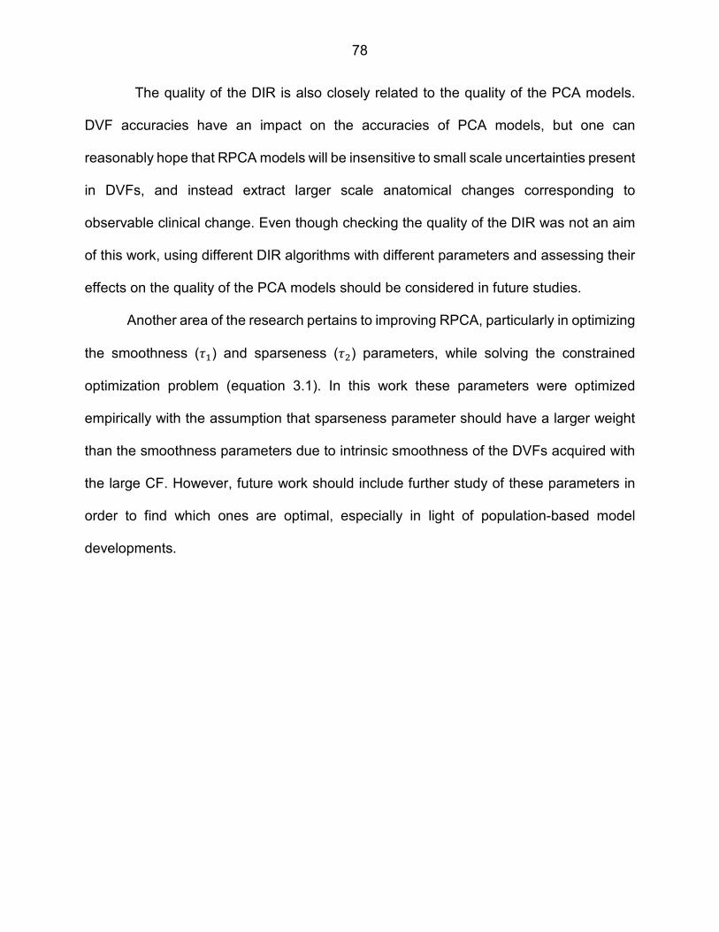
78

The quality of the DIR is also closely related to the quality of the PCA models.

DVF accuracies have an impact on the accuracies of PCA models, but one can

reasonably hope that RPCA models will be insensitive to small scale uncertainties present

in DVFs, and instead extract larger scale anatomical changes corresponding to

observable clinical change. Even though checking the quality of the DIR was not an aim

of this work, using different DIR algorithms with different parameters and assessing their

effects on the quality of the PCA models should be considered in future studies.

Another area of the research pertains to improving RPCA, particularly in optimizing

the smoothness (i�) and sparseness (i() parameters, while solving the constrained

optimization problem (equation 3.1). In this work these parameters were optimized

empirically with the assumption that sparseness parameter should have a larger weight

than the smoothness parameters due to intrinsic smoothness of the DVFs acquired with

the large CF. However, future work should include further study of these parameters in

order to find which ones are optimal, especially in light of population-based model

developments.

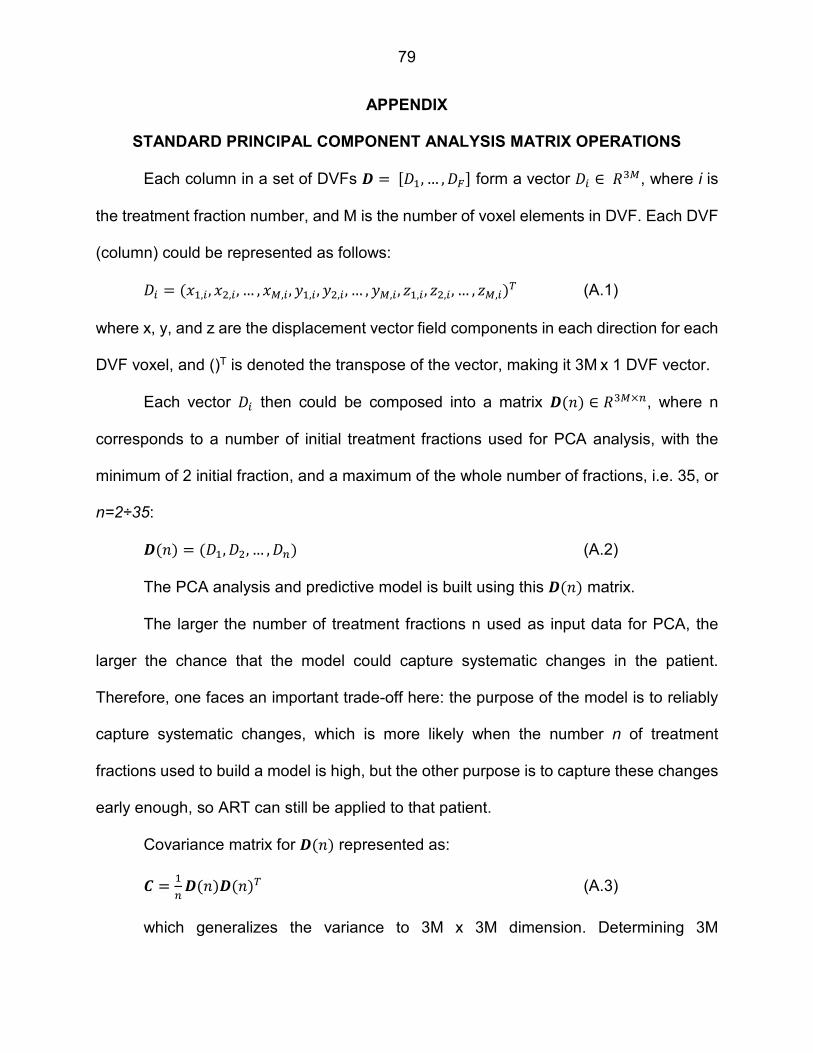
79

APPENDIX

STANDARD PRINCIPAL COMPONENT ANALYSIS MATRIX OPERATIONS

Each column in a set of DVFs � = . �, … , Y0 form a vector � ∈ � _, where i is

the treatment fraction number, and M is the number of voxel elements in DVF. Each DVF

(column) could be represented as follows:

� = $A�,�, A(,�, … , A_,�, l�,�, l(,�, … , l_,�, m�,�, m(,�, … , m_,�'� (A.1)

where x, y, and z are the displacement vector field components in each direction for each

DVF voxel, and ()T is denoted the transpose of the vector, making it 3M x 1 DVF vector.

Each vector � then could be composed into a matrix �$�' ∈ � _×�, where n

corresponds to a number of initial treatment fractions used for PCA analysis, with the

minimum of 2 initial fraction, and a maximum of the whole number of fractions, i.e. 35, or

n=2÷35:

�$�' = $ �, (, … , �' (A.2)

The PCA analysis and predictive model is built using this �$�' matrix.

The larger the number of treatment fractions n used as input data for PCA, the

larger the chance that the model could capture systematic changes in the patient.

Therefore, one faces an important trade-off here: the purpose of the model is to reliably

capture systematic changes, which is more likely when the number n of treatment

fractions used to build a model is high, but the other purpose is to capture these changes

early enough, so ART can still be applied to that patient.

Covariance matrix for �$�' represented as:

� = �� �$�'�$�'� (A.3)

which generalizes the variance to 3M x 3M dimension. Determining 3M

80

eigenvalues and 3M corresponding eigenvectors is a complex, intractable and, after all,

unnecessary task. There are computationally more feasible and much faster methods to

find these. This alternative method is useful when the number of measurements is much

less than number of dimensions, or n<<M.

First, substitute A.3 into the eigenvector equation:

�� �$�'�$�'��$�' = ��$�' (A.4)

�$�' represent eigenvectors for the covariance matrix C, and � are the

corresponding eigenvalues.

Multiplying both sides of A.4 by �$�'� and defining �$�' = �$�'��$�' gives us:

�� �$�'��$�'�$�' = ��$�' (A.5)

A.5 is a reformed equation which gives us eigenvalues and eigenvectors of smaller

matrix of the size n x n: �$�'��$�'.

Multiplying both sides of A.5 by �$�':

�� �$�'�$�'�$�$�'�$�'' = �$�$�'�$�'' (A.6)

Thus from A.5 it follows that eigenvectors for the covariance matrix С defined in

A.3:

��$�' = ����� �$�'��$�' (A.7)

Where the factor �

���� is used to renormalize the eigenvector ��$�', such as

‖��$�'‖ = 1.

These eigenvectors ��$�' are defined as EDVFs in this work and they represent

mutually independent vector fields with the maximum number of meaningful EDVFs n-1

(one of the EDVFs corresponds to the zero eigenvalue and is not meaningful).

81

Thus, the matrix of meaningful EDVFs has the form �$�' ∈ ��g×$��f', where each

column represents each EDVFi, and the EDVF1 corresponds to the largest eigenvalue

positioned at the first column of �$�', the EDVF2 corresponds to the second largest

eigenvalue, etc.

82

REFERENCES

1 J.M. Wilkinson, "Geometric uncertainties in radiotherapy," Br J Radiol 77, 86-87

(2004).

2 C.W. Hurkmans, P. Remeijer, J.V. Lebesque, B.J. Mijnheer, "Set-up verification

using portal imaging; review of current clinical practice," Radiother Oncol 58, 105-

120 (2001).

3 C.S. Chui, E. Yorke, L. Hong, "The effects of intra-fraction organ motion on the

delivery of intensity-modulated field with a multileaf collimator," Med Phys 30,

1736-1746 (2003).

4 S. Webb, "Motion effects in (intensity modulated) radiation therapy: a review," Phys

Med Biol 51, R403-425 (2006).

5 R. Varadhan, S.K. Hui, S. Way, K. Nisi, "Assessing prostate, bladder and rectal

doses during image guided radiation therapy--need for plan adaptation?," J Appl

Clin Med Phys 10, 2883 (2009).

6 Z. Gao, D. Wilkins, L. Eapen, C. Morash, Y. Wassef, L. Gerig, "A study of prostate

delineation referenced against a gold standard created from the visible human

data," Radiother Oncol 85, 239-246 (2007).

7 C.F. Njeh, "Tumor delineation: The weakest link in the search for accuracy in

radiotherapy," J Med Phys 33, 136-140 (2008).

8 C. Rasch, R. Steenbakkers, M. van Herk, "Target definition in prostate, head, and

neck," Semin Radiat Oncol 15, 136-145 (2005).

9 A. Isambert, F. Dhermain, F. Bidault, O. Commowick, P.Y. Bondiau, G. Malandain,

D. Lefkopoulos, "Evaluation of an atlas-based automatic segmentation software

83

for the delineation of brain organs at risk in a radiation therapy clinical context,"

Radiother Oncol 87, 93-99 (2008).

10 J.L. Barker, Jr., A.S. Garden, K.K. Ang, J.C. O'Daniel, H. Wang, L.E. Court, W.H.

Morrison, D.I. Rosenthal, K.S. Chao, S.L. Tucker, R. Mohan, L. Dong,

"Quantification of volumetric and geometric changes occurring during fractionated

radiotherapy for head-and-neck cancer using an integrated CT/linear accelerator

system," Int J Radiat Oncol Biol Phys 59, 960-970 (2004).

11 P. Castadot, X. Geets, J.A. Lee, N. Christian, V. Gregoire, "Assessment by a

deformable registration method of the volumetric and positional changes of target

volumes and organs at risk in pharyngo-laryngeal tumors treated with concomitant

chemo-radiation," Radiother Oncol 95, 209-217 (2010).

12 J.D. Chencharick, K.L. Mossman, "Nutritional consequences of the radiotherapy

of head and neck cancer," Cancer 51, 811-815 (1983).

13 S.S. Donaldson, R.A. Lenon, "Alterations of nutritional status: impact of

chemotherapy and radiation therapy," Cancer 43, 2036-2052 (1979).

14 C. Lee, K.M. Langen, W. Lu, J. Haimerl, E. Schnarr, K.J. Ruchala, G.H. Olivera,

S.L. Meeks, P.A. Kupelian, T.D. Shellenberger, R.R. Manon, "Evaluation of

geometric changes of parotid glands during head and neck cancer radiotherapy

using daily MVCT and automatic deformable registration," Radiother Oncol 89, 81-

88 (2008).

15 "ICRU Report 50—Prescribing, Recording and Reporting Photon Beam Therapy |

Browse - Medical Physics," 1994).

84

16 "ICRU Report 62 - Prescribing, Recording and Reporting Photon Beam Therapy

(Supplement to ICRU Report 50)," 2000).

17 M. van Herk, P. Remeijer, J.V. Lebesque, "Inclusion of geometric uncertainties in

treatment plan evaluation," Int J Radiat Oncol Biol Phys 52, 1407-1422 (2002).

18 M.R. Button, C.A. Morgan, E.S. Croydon, S.A. Roberts, T.D. Crosby, "Study to

determine adequate margins in radiotherapy planning for esophageal carcinoma

by detailing patterns of recurrence after definitive chemoradiotherapy," Int J Radiat

Oncol Biol Phys 73, 818-823 (2009).

19 L. Ekberg, O. Holmberg, L. Wittgren, G. Bjelkengren, T. Landberg, "What margins

should be added to the clinical target volume in radiotherapy treatment planning

for lung cancer?," Radiother Oncol 48, 71-77 (1998).

20 S.W. Lee, B.A. Fraass, L.H. Marsh, K. Herbort, S.S. Gebarski, M.K. Martel, E.H.

Radany, A.S. Lichter, H.M. Sandler, "Patterns of failure following high-dose 3-D

conformal radiotherapy for high-grade astrocytomas: a quantitative dosimetric

study," Int J Radiat Oncol Biol Phys 43, 79-88 (1999).

21 L.P. Muren, R. Smaaland, O. Dahl, "Organ motion, set-up variation and treatment

margins in radical radiotherapy of urinary bladder cancer," Radiother Oncol 69,

291-304 (2003).

22 M. van Herk, P. Remeijer, C. Rasch, J.V. Lebesque, "The probability of correct

target dosage: dose-population histograms for deriving treatment margins in

radiotherapy," Int J Radiat Oncol Biol Phys 47, 1121-1135 (2000).

23 J.C. Stroom, B.J. Heijmen, "Limitations of the planning organ at risk volume (PRV)

concept," Int J Radiat Oncol Biol Phys 66, 279-286 (2006).

85

24 L.B. Marks, E.D. Yorke, A. Jackson, R.K. Ten Haken, L.S. Constine, A. Eisbruch,

S.M. Bentzen, J. Nam, J.O. Deasy, "Use of Normal Tissue Complication Probability

Models in the Clinic," Int J Radiat Oncol 76, S10-S19 (2010).

25 D.A. Jaffray, P.E. Lindsay, K.K. Brock, J.O. Deasy, W.A. Tome, "Accurate

accumulation of dose for improved understanding of radiation effects in normal

tissue," Int J Radiat Oncol Biol Phys 76, S135-139 (2010).

26 L.F. Cazzaniga, M.A. Marinoni, A. Bossi, E. Bianchi, E. Cagna, D. Cosentino, L.

Scandolaro, M. Valli, M. Frigerio, "Interphysician variability in defining the planning

target volume in the irradiation of prostate and seminal vesicles," Radiother Oncol

47, 293-296 (1998).

27 C.H. Ketting, M. Austin-Seymour, I. Kalet, J. Unger, S. Hummel, J. Jacky,

"Consistency of three-dimensional planning target volumes across physicians and

institutions," Int J Radiat Oncol Biol Phys 37, 445-453 (1997).

28 H. Vorwerk, G. Beckmann, M. Bremer, M. Degen, B. Dietl, R. Fietkau, T. Gsanger,

R.M. Hermann, M.K. Alfred Herrmann, U. Holler, M. van Kampen, W. Korber, B.

Maier, T. Martin, M. Metz, R. Richter, B. Siekmeyer, M. Steder, D. Wagner, C.F.

Hess, E. Weiss, H. Christiansen, "The delineation of target volumes for

radiotherapy of lung cancer patients," Radiother Oncol 91, 455-460 (2009).

29 L. Xing, B. Thorndyke, E. Schreibmann, Y. Yang, T.F. Li, G.Y. Kim, G. Luxton, A.

Koong, "Overview of image-guided radiation therapy," Med Dosim 31, 91-112

(2006).

86

30 T. Li, X. Zhu, D. Thongphiew, W.R. Lee, Z. Vujaskovic, Q. Wu, F.F. Yin, Q.J. Wu,

"On-line adaptive radiation therapy: feasibility and clinical study," J Oncol 2010,

407236 (2010).

31 D. Yan, F. Vicini, J. Wong, A. Martinez, "Adaptive radiation therapy," Phys Med

Biol 42, 123-132 (1997).

32 K.S. Chao, D.A. Low, C.A. Perez, J.A. Purdy, "Intensity-modulated radiation

therapy in head and neck cancers: The Mallinckrodt experience," Int J Cancer 90,

92-103 (2000).

33 K.S. Chao, G. Ozyigit, B.N. Tran, M. Cengiz, J.F. Dempsey, D.A. Low, "Patterns

of failure in patients receiving definitive and postoperative IMRT for head-and-neck

cancer," Int J Radiat Oncol Biol Phys 55, 312-321 (2003).

34 A. Eisbruch, R.K. Ten Haken, H.M. Kim, L.H. Marsh, J.A. Ship, "Dose, volume,

and function relationships in parotid salivary glands following conformal and

intensity-modulated irradiation of head and neck cancer," Int J Radiat Oncol Biol

Phys 45, 577-587 (1999).

35 N. Lee, P. Xia, N.J. Fischbein, P. Akazawa, C. Akazawa, J.M. Quivey, "Intensity-

modulated radiation therapy for head-and-neck cancer: the UCSF experience

focusing on target volume delineation," Int J Radiat Oncol Biol Phys 57, 49-60

(2003).

36 C. Han, Y.J. Chen, A. Liu, T.E. Schultheiss, J.Y. Wong, "Actual dose variation of

parotid glands and spinal cord for nasopharyngeal cancer patients during

radiotherapy," Int J Radiat Oncol Biol Phys 70, 1256-1262 (2008).

87

37 J.C. O'Daniel, A.S. Garden, D.L. Schwartz, H. Wang, K.K. Ang, A. Ahamad, D.I.

Rosenthal, W.H. Morrison, J.A. Asper, L. Zhang, S.M. Tung, R. Mohan, L. Dong,

"Parotid gland dose in intensity-modulated radiotherapy for head and neck cancer:

is what you plan what you get?," Int J Radiat Oncol Biol Phys 69, 1290-1296

(2007).

38 J. Wang, S. Bai, N. Chen, F. Xu, X. Jiang, Y. Li, Q. Xu, Y. Shen, H. Zhang, Y.

Gong, R. Zhong, Q. Jiang, "The clinical feasibility and effect of online cone beam

computer tomography-guided intensity-modulated radiotherapy for

nasopharyngeal cancer," Radiother Oncol 90, 221-227 (2009).

39 D.L. Schwartz, A.S. Garden, S.J. Shah, G. Chronowski, S. Sejpal, D.I. Rosenthal,

Y. Chen, Y. Zhang, L. Zhang, P.F. Wong, J.A. Garcia, K. Kian Ang, L. Dong,

"Adaptive radiotherapy for head and neck cancer--dosimetric results from a

prospective clinical trial," Radiother Oncol 106, 80-84 (2013).

40 E. Budiarto, M. Keijzer, P.R. Storchi, M.S. Hoogeman, L. Bondar, T.F. Mutanga,

H.C. de Boer, A.W. Heemink, "A population-based model to describe geometrical

uncertainties in radiotherapy: applied to prostate cases," Phys Med Biol 56, 1045-

1061 (2011).

41 E. Fontenla, C.A. Pelizzari, J.C. Roeske, G.T. Chen, "Using serial imaging data to

model variabilities in organ position and shape during radiotherapy," Phys Med

Biol 46, 2317-2336 (2001).

42 M.S. Hoogeman, M. van Herk, D. Yan, L.J. Boersma, P.C. Koper, J.V. Lebesque,

"A model to simulate day-to-day variations in rectum shape," Int J Radiat Oncol

Biol Phys 54, 615-625 (2002).

88

43 G.S. Mageras, G.J. Kutcher, S.A. Leibel, M.J. Zelefsky, E. Melian, R. Mohan, Z.

Fuks, "A method of incorporating organ motion uncertainties into three-

dimensional conformal treatment plans," Int J Radiat Oncol Biol Phys 35, 333-342

(1996).

44 T.F. Mutanga, H.C. de Boer, G.J. van der Wielen, M.S. Hoogeman, L. Incrocci,

B.J. Heijmen, "Margin evaluation in the presence of deformation, rotation, and

translation in prostate and entire seminal vesicle irradiation with daily marker-

based setup corrections," Int J Radiat Oncol Biol Phys 81, 1160-1167 (2011).

45 M. Sohn, M. Birkner, D. Yan, M. Alber, "Modelling individual geometric variation

based on dominant eigenmodes of organ deformation: implementation and

evaluation," Phys Med Biol 50, 5893-5908 (2005).

46 D. Yan, D.A. Jaffray, J.W. Wong, "A model to accumulate fractionated dose in a

deforming organ," Int J Radiat Oncol Biol Phys 44, 665-675 (1999).

47 M. Sohn, B. Sobotta, M. Alber, "Dosimetric treatment course simulation based on

a statistical model of deformable organ motion," Phys Med Biol 57, 3693-3709

(2012).

48 I.T. Jolliffe, Principal component analysis, 2nd ed. (Springer, New York, 2002).

49 G.J. Price, C.J. Moore, "A method to calculate coverage probability from

uncertainties in radiotherapy via a statistical shape model," Phys Med Biol 52,

1947-1965 (2007).

50 Q. Zhang, A. Pevsner, A. Hertanto, Y.C. Hu, K.E. Rosenzweig, C.C. Ling, G.S.

Mageras, "A patient-specific respiratory model of anatomical motion for radiation

treatment planning," Med Phys 34, 4772-4781 (2007).

89

51 V. Pekar, T.R. McNutt, M.R. Kaus, "Automated model-based organ delineation for

radiotherapy planning in prostatic region," Int J Radiat Oncol Biol Phys 60, 973-

980 (2004).

52 D. Merck, G. Tracton, R. Saboo, J. Levy, E. Chaney, S. Pizer, S. Joshi, "Training

models of anatomic shape variability," Med Phys 35, 3584-3596 (2008).

53 K. Pearson, "LIII. On lines and planes of closest fit to systems of points in space,"

Philosophical Magazine Series 6 2, 559-572 (1901).

54 K.T. Gribbon, C.T. Johnston, D.G. Bailey, A Real-time FPGA Implementation of a

Barrel Distortion Correction Algorithm with Bilinear Interpolation.

55 GNU Scientific Library - GNU Project - Free Software Foundation,

http://www.gnu.org/software/gsl/

56 J.P. Thirion, presented at the Computer Vision and Pattern Recognition, 1996.

Proceedings CVPR '96, 1996 IEEE Computer Society Conference on1996

(unpublished).

57 T. Vercauteren, X. Pennec, A. Perchant, N. Ayache, "Non-parametric

Diffeomorphic Image Registration with the Demons Algorithm," in Medical Image

Computing and Computer-Assisted Intervention – MICCAI 2007: 10th International

Conference, Brisbane, Australia, October 29 - November 2, 2007, Proceedings,

Part II, edited by N. Ayache, S. Ourselin, A. Maeder (Springer Berlin Heidelberg,

Berlin, Heidelberg, 2007), pp. 319-326.

58 T. Vercauteren, X. Pennec, A. Perchant, N. Ayache, "Diffeomorphic demons:

efficient non-parametric image registration," NeuroImage 45, S61-72 (2009).

90

59 D. Yang, S. Brame, I. El Naqa, A. Aditya, Y. Wu, S.M. Goddu, S. Mutic, J.O. Deasy,

D.A. Low, "Technical note: DIRART--A software suite for deformable image

registration and adaptive radiotherapy research," Med Phys 38, 67-77 (2011).

60 D.A. Low, W.B. Harms, S. Mutic, J.A. Purdy, "A technique for the quantitative

evaluation of dose distributions," Med Phys 25, 656-661 (1998).

61 W.-T. Wang, H.-C. Huang, "Regularized Principal Component Analysis for Spatial

Data," in ArXiv e-prints, Vol. 1501 (2015).

62 H. Xu, D.J. Vile, M. Sharma, J.J. Gordon, J.V. Siebers, "Coverage-based treatment

planning to accommodate deformable organ variations in prostate cancer

treatment," Med Phys 41, 101705 (2014).

63 X. Nie, J. Liang, D. Yan, "Organ sample generator for expected treatment dose

construction and adaptive inverse planning optimization," Med Phys 39, 7329-

7337 (2012).

64 D.L. Schwartz, "Current progress in adaptive radiation therapy for head and neck

cancer," Curr Oncol Rep 14, 139-147 (2012).

65 C. Veiga, J. McClelland, S. Moinuddin, A. Lourenco, K. Ricketts, J. Annkah, M.

Modat, S. Ourselin, D. D'Souza, G. Royle, "Toward adaptive radiotherapy for head

and neck patients: Feasibility study on using CT-to-CBCT deformable registration

for "dose of the day" calculations," Med Phys 41, 031703 (2014).

66 ITK - Insight Segmentation and Registration Toolkit, https://itk.org/

67 A. Kumarasiri, C. Liu, F. Siddiqui, H. Zhong, I.J. Chetty, J. Kim, "Target and organ

dose estimation from intensity modulated head and neck radiation therapy using 3

deformable image registration algorithms," Pract Radiat Oncol 5, e317-325 (2015).

91

ABSTRACT

PCA-BASED ANATOMICAL MOTION MODELS FOR USING IN ADAPTIVE RADIATION THERAPY OF HEAD AND NECK CANCER PATIENTS

by

MIKHAIL A. CHETVERTKOV

August 2016

Advisor: Dr. Indrin J. Chetty

Major: Medical Physics

Degree: Doctor of Philosophy

Purpose: To develop standard and regularized principal component analysis

(PCA) models of anatomical changes from daily cone beam CTs (CBCTs) of head and

neck (H&N) patients, assess their potential use in adaptive radiation therapy (ART), and

to extract quantitative information for treatment response assessment.

Methods: Planning CT (pCT) images of H&N patients were artificially deformed to

create “digital phantom” images, which modeled systematic anatomical changes during

Radiation Therapy (RT). Artificial deformations closely mirrored patients’ actual

deformations, and were interpolated to generate 35 synthetic CBCTs, representing

evolving anatomy over 35 fractions. Deformation vector fields (DVFs) were acquired

between pCT and synthetic CBCTs (i.e., digital phantoms), and between pCT and clinical

CBCTs. Patient-specific standard PCA (SPCA) and regularized PCA (RPCA) models

were built from these synthetic and clinical DVF sets. Eigenvectors, or eigenDVFs

(EDVFs), having the largest eigenvalues were hypothesized to capture the major

92

anatomical deformations during treatment. Modeled anatomies were used to assess the

dose deviations with respect to the planned dose distribution.

Results: PCA models achieve variable results, depending on the size and location

of anatomical change. Random changes prevent or degrade SPCA’s ability to detect

underlying systematic change. RPCA is able to detect smaller systematic changes

against the background of random fraction-to-fraction changes, and is therefore more

successful than SPCA at capturing systematic changes early in treatment. SPCA models

were less successful at modeling systematic changes in clinical patient images, which

contain a wider range of random motion than synthetic CBCTs, while the regularized

approach was able to extract major modes of motion. For dose assessment it has been

shown that the modeled dose distribution was different from the planned dose for the

parotid glands due to their shrinkage and shift into the higher dose volumes during the

radiotherapy course. Modeled DVHs still underestimated the effect of parotid shrinkage

due to the large compression factor (CF) used to acquire DVFs.

Conclusion: Leading EDVFs from both PCA approaches have the potential to

capture systematic anatomical changes during H&N radiotherapy when systematic

changes are large enough with respect to random fraction-to-fraction changes. In all

cases the RPCA approach appears to be more reliable than SPCA at capturing

systematic changes, enabling dosimetric consequences to be projected to the future

treatment fractions based on trends established early in a treatment course, or,

potentially, based on population models. This work showed that PCA has a potential in

identifying the major mode of anatomical changes during the radiotherapy course and

93

subsequent use of this information in future dose predictions is feasible. Use of smaller

CF values for DVFs is preferred, otherwise anatomical motion will be underestimated.

94

AUTOBIOGRAPHICAL STATEMENT MIKHAIL A. CHETVERTKOV

EDUCATION 2011-2016 Ph.D. Medical Physics, Wayne State University, Detroit, MI 2009-2011 Honors M.S. Physics, Moscow State University, Moscow, Russia 2005-2009 B.S. Physics, Moscow State University, Moscow, Russia

CERTIFICATION 2013 American Board of Radiology Part 1

PROFESSIONAL APPOINTMENTS 2011-2016 Graduate Research Assistant, Henry Ford Health System Department of Radiation Oncology, Detroit, MI 2008-2011 Junior Research Scientist, Department of Atomic Physics and Quantum Theory of Collisions, Moscow State University, Moscow, Russia

ACADEMIC AND PROFESSIONAL MEMBERSHIPS 2013- American Association of Physicists in Medicine, Great Lakes Chapter 2011- American Association of Physicists in Medicine

COMMITTEE APPOINTMENTS 2015- AAPM Working Group on Student and Trainee Research: Member

PUBLICATIONS 1. M.A. Chetvertkov, F. Siddiqui, J. Kim, I.J. Chetty, A. Kumarasiri, C. Liu, J.J.

Gordon, “Use of Regularized Principal Component Analysis to Model Anatomical Changes During Head and Neck Radiation Therapy for Treatment Adaptation and Response Assessment”, Accepted: Med. Phys. (2016).

2. C. Liu, A. Kumarasiri, M. Kamal, M.A. Chetvertkov, J. Gordon, H. Zhong, F. Siddiqui, I.J. Chetty, J. Kim, "An automatic dosimetric and geometric tracking system for head and neck adaptive radiotherapy," in World Congress on Medical Physics and Biomedical Engineering, June 7-12, 2015, Toronto, Canada, edited by A.D. Jaffray (Springer International Publishing, Cham, 2015), pp. 570-574.

3. M.A. Chetvertkov, V.A. Chetvertkova, M.B. Nurusheva, S.B. Nurushev, A.V. Ridiger, "Helicity conservation hypothesis and pp-elastic scattering," Physics of Particles and Nuclei 45, 99-101 (2014).

4. E. Mayyas, I.J. Chetty, M.A. Chetvertkov, N. Wen, T. Neicu, T. Nurushev, L. Ren, M. Lu, H. Stricker, D. Pradhan, B. Movsas, M.A. Elshaikh, "Evaluation of multiple image-based modalities for image-guided radiation therapy (IGRT) of prostate carcinoma: a prospective study," Med Phys 40, 041707 (2013).