preparatory signal detection for the eu member states ... · pdf file–6.3 percentage...
TRANSCRIPT
Preparatory Signal Detection for the EU Member States under EU Burden Sharing - Advanced Monitoring Including Uncertainty (1990-2002)
Jonas, M., Nilsson, S., Bun, R., Dachuk, V., Gusti, M., Horabik, J., Jeda, W. and Nahorski, Z.
IIASA Interim ReportSeptember 2004
Jonas, M., Nilsson, S., Bun, R., Dachuk, V., Gusti, M., Horabik, J., Jeda, W. and Nahorski, Z. (2004) Preparatory Signal
Detection for the EU Member States under EU Burden Sharing - Advanced Monitoring Including Uncertainty (1990-2002).
IIASA Interim Report. IIASA, Laxenburg, Austria, IR-04-046 Copyright © 2004 by the author(s). http://pure.iiasa.ac.at/7402/
Interim Reports on work of the International Institute for Applied Systems Analysis receive only limited review. Views or
opinions expressed herein do not necessarily represent those of the Institute, its National Member Organizations, or other
organizations supporting the work. All rights reserved. Permission to make digital or hard copies of all or part of this work
for personal or classroom use is granted without fee provided that copies are not made or distributed for profit or commercial
advantage. All copies must bear this notice and the full citation on the first page. For other purposes, to republish, to post on
servers or to redistribute to lists, permission must be sought by contacting [email protected]

International Institute for Applied Systems Analysis Schlossplatz 1 A-2361 Laxenburg, Austria
Tel: +43 2236 807 342Fax: +43 2236 71313
E-mail: [email protected]: www.iiasa.ac.at
Interim Reports on work of the International Institute for Applied Systems Analysis receive only limited review. Views or opinions expressed herein do not necessarily represent those of the Institute, its National Member Organizations, or other organizations supporting the work.
Interim Report IR-04-046
Preparatory Signal Detection for the EU Member States Under EU Burden Sharing ― Advanced Monitoring Including Uncertainty (1990–2002)
Matthias Jonas ([email protected]) Sten Nilsson ([email protected]) Rostyslav Bun ([email protected]) Volodymyr Dachuk ([email protected]) Mykola Gusti ([email protected]) Joanna Horabik ([email protected]) Waldemar Jęda ([email protected]) Zbigniew Nahorski ([email protected])
Approved by
Leen Hordijk Director, IIASA
15 September 2004

ii
Contents
1 BACKGROUND AND OBJECTIVE 1
2 METHODOLOGY 7
3 RESULTS 11
4 INTERPRETATION OF RESULTS AND CONCLUSIONS 19
REFERENCES 27
ACRONYMS AND NOMENCLATURE 28
ISO COUNTRY CODE 29

iii
Abstract
This study follows up the authors’ collaborative IIASA Interim Report IR-04-024
(Jonas et al., 2004a), which addresses the preparatory detection of uncertain greenhouse
gas (GHG) emission changes (also termed emission signals) under the Kyoto Protocol.
The question probed was how well do we need to know net emissions if we want to
detect a specified emission signal after a given time? The authors used the Protocol’s
Annex I countries as net emitters and excluded the emissions/removals due to land-use
change and forestry (LUCF). They motivated the application of preparatory signal
detection in the context of the Kyoto Protocol as a necessary measure that should have
been taken prior to/in negotiating the Protocol. The authors argued that uncertainties are
already monitored and are increasingly made available but that monitored emissions and
uncertainties are still dealt with in isolation. A connection between emission and (total)
uncertainty estimates for the purpose of an advanced country evaluation has not yet
been established. The authors developed four preparatory signal detection techniques
and applied these to the Annex I countries under the Kyoto Protocol. The frame of
reference for preparatory signal detection is that Annex I countries comply with their
committed emission targets in 2008–2012.
In our study we apply one of these techniques, the combined undershooting and
verification time (Und&VT) concept to advance the monitoring of the GHG emissions
reported by the Member States of the European Union (EU). In contrast to the earlier
study, we focus on the Member States’ committed emission targets under the EU burden
sharing in compliance with the Kyoto Protocol. We apply the Und&VT concept in a
standard mode, i.e., with reference to the Member States committed emission targets in
2008–2012, and in a new mode, i.e., with reference to linear path emission targets
between the base year and the commitment year (here for 2002).
To advance the reporting of the EU we take uncertainty and its consequences into
consideration, i.e., (i) the risk that a Member State’s true emissions in the commitment
year/period are above its true emission limitation or reduction commitment; and (ii) the
detectability of its target. Undershooting the committed EU target or EU-compatible,
but detectable, target can decrease this risk. We contrast the Member States’ linear path
undershooting targets for the year 2002 with their actual emission situation in that year,
for which we use the distance-to-target indicator (DTI) introduced by the European
Environment Agency.
In 2002 only four countries exhibit a negative DTI and thus appear as potential sellers:
France, Germany, Sweden and the United Kingdom. However, expecting that the EU
Member States exhibit relative uncertainties in the range of 5–10% and above rather
than below, excluding emissions/removals due to LUCF, the Member States require

iv
considerable undershooting of their EU-compatible, but detectable, targets if one wants
to keep the associated risk low ( 0.1α≈ ). These conditions can only be met by two
Member States, Germany and the United Kingdom, while Sweden and France can only
act as potential high-risk sellers (ranked in terms of creditability). In contrast, with
relative uncertainty increasing from 5 to 10%, the emission signal of the EU as a whole
switches from “detectable” to “non-detectable”, indicating that the negotiations for the
Kyoto Protocol were imprudent because they did not take uncertainty and its
consequences into account.
We anticipate that the evaluation of emission signals in terms of risk and detectability
will become standard practice and that these two qualifiers will be accounted for in
pricing GHG emission permits.

v
Acknowledgments
This report follows up the research project Carbon Management ― Uncertainty and
Verification that was carried out for and funded by the Austrian Federal Ministry for
Education, Science and Culture (Ref.: GZ 309.012/1-VIII/B-8a/2000). We particularly
thank Gisela Zieger for her support during this project.
This report benefited greatly from complementary research that is or has been carried
out in Poland and the Ukraine, in Poland under the project Uncertainty, Verification,
and Risk Management under the Kyoto Protocol financially supported by the Polish
State Committee for Scientific Research (Ref: 3 P04G 120 24) and in the Ukraine under
the project Information Technologies for Greenhouse Gas Inventories and Prognosis of
the Carbon Budget of Ukraine funded by the Science and Technology Center in Ukraine
(Ref.: 1700).
The authors are especially indebted to Shari Jandl for her assistance on improving and
finalizing the manuscript.

vi
About the Authors
Matthias Jonas is a Research Scholar in IIASA’s Forestry Program and Sten Nilsson is
Deputy Director of IIASA as well as Leader of the Forestry Program.
Rostyslav Bun, Volodymyr Dachuk and Mykola Gusti are from the State Scientific and
Research Institute of Information Infrastructure (SSRIII) in Lviv, Ukraine. Rostyslav
Bun is Deputy Director of Science and Research and Leader of the Department of
Information Technologies for Mathematical Modeling of Complex Systems and
Phenomena. Volodymyr Dachuk and Mykola Gusti are Senior Research Scientists at
the Department of Mathematical Modeling of Complex Systems and Phenomena.
Joanna Horabik, Waldemar Jęda and Zbigniew Nahorski are from the Systems Research
Institute (SRI) of the Polish Academy of Sciences in Warsaw. Joanna Horabik is a
research assistant in the Laboratory of Computer Modeling, Waldemar Jęda is an
adjunct in the Laboratory of Computer Modeling at SRI as well as in the Warsaw
School of Information Technology, Faculty of Computer Science, and Zbigniew
Nahorski is Head of the Laboratory of Computer Models at SRI as well as Dean of the
Department of Informatics at the Warsaw School of Information Technology.

1
Preparatory Signal Detection for the EU Member States Under EU Burden Sharing ― Advanced Monitoring Including Uncertainty (1990–2002)
Matthias Jonas, Sten Nilsson, Rostyslav Bun, Volodymyr Dachuk, Mykola Gusti, Joanna Horabik, Waldemar Jęda and Zbigniew Nahorski
1 Background and Objective
This study follows up the authors’ collaborative IIASA Interim Report IR-04-024
(Jonas et al., 2004a). It applies the strictest of the preparatory signal detection
techniques developed in this report, the combined undershooting and verification time
(Und&VT) concept, to advance the monitoring of the greenhouse gas (GHG) emissions
reported by the Member States of the European Union (EU) under EU burden sharing in
compliance with the Kyoto Protocol. Under current monitoring, the Member States’
emissions are evaluated in relation to the EU’s actual (here: 2002) target and in terms of
their positive and negative contributions to this target.1 This monitoring process is
illustrated in Figures 1 and 2 and Table 1. They give details, for each Member State and
the EU as a whole, of trends in emissions of GHGs (CO2, CH4, N2O, HFCs, PFCs, SF6)
up to 2002.2 Figure 1 follows the total emissions of the EU over time since 1990, while
the distance-to-target indicator (DTI) introduced in Figure 2, based on the country data
listed in Table 1, is a measure of the derivation of actual GHG emissions in 2002 from
the linear target path between 1990 and the EU target for 2008–2012, assuming that
only domestic measures will be used. A negative DTI means that a Member State is
below its linear target path, a positive DTI that a Member State is above its linear target
path (EEA, 2003, 2004; Gugele et al., 2004)3. As Figures 1 and 2 only present relative
information of the kind “can sell versus must buy”, we add Figure 3, which translates
this information into absolute numbers based on the Member States’ emissions in 2002
(Table 1) and their DTIs for that year. Figure 3 helps us to understand the 2002 situation
of the EU in quantitative terms.
1 In a recent study, the authors evaluated the Member States’ emissions in relation to the EU’s 2001 target
(Jonas et al., 2004b). 2 Emissions from international aviation and shipping, and emissions/removals due to land-use change and
forestry (LUCF), are not covered (EEA, 2004). 3 For example, Ireland is allowed a 13% increase from 1990 levels by 2008–2012, so its theoretical
“linear target” for 2002 is a rise of no more than 7.8%. Its actual emissions in 2002 show an increase of
28.9% since 1990; hence, its “distance-to-target” is 28.9 – 7.8, or 21.1 percentage points. Germany’s
Kyoto target is a 21% reduction, so its theoretical “linear target” for 2002 is a decrease of 12.6%. Actual
emissions in 2002 were 18.9% lower than in 1990; hence, its “distance-to-target” is (–18.9) – (–12.6), or
–6.3 percentage points (EEA, 2003, 2004; Gugele et al., 2004).

2
Figure 1: Total EU GHG emissions for 1990–2002 in relation to the Kyoto target for
2008–12. Source: EEA (2004:Figure 1).
1)
Denmark’s DTI is +3.5 percentage points if its emissions are adjusted for electricity
trade in 1990. 2)
The Dutch DTI is –1.4 percentage points, putting it on track to meet its Kyoto target, if
anticipated emission savings from use of the Kyoto mechanisms are taken into account.
The Netherlands is the only country that has provided detailed information on financial
resources earmarked for using the mechanisms, specific projects and quantified emission
reductions.
Figure 2: Distance-to-target indicator (DTI) for EU Member States in 2002 (in
consideration of the EU burden sharing targets under the Kyoto Protocol).
Source: Modified from EEA (2004:Figure 2).

3
Table 1: 2008–2012 targets for EU Member States under the Kyoto Protocol and EU
burden sharing. Source: Modified from Gugele et al. (2004:Table ES.4).
Member State
Base Yeara
(million tonnes)
2002
(million tonnes)
Change
2001–2002
(%)
Change Base
Year–2002
(%)
Targets 2008–12 under
EU burden sharing
(%)
Austria 78.0 84.6 0.3 8.5 -13.0
Belgium 146.8 150.0 0.5 2.1 -7.5
Denmarkb 69.0 68.5 -1.2 -0.8 (-9.1) -21.0
Finland 76.8 82.0 1.7 6.8 0.0
France 564.7 553.9 -1.4 -1.9 0.0
Germany 1253.3 1016.0 -1.1 -18.9 -21.0
Greece 107.0 135.4 0.3 26.5 25.0
Ireland 53.4 68.9 -1.6 28.9 13.0
Italy 508.0 553.8 -0.1 9.0 -6.5
Luxembourg 12.7 10.8 10.4 -15.1 -28.0
Netherlands 212.5 213.8 -1.1 0.6 -6.0
Portugal 57.9 81.6 4.1 41.0 27.0
Spain 286.8 399.7 4.2 39.4 15.0
Sweden 72.3 69.6 2.0 -3.7 4.0
United Kingdom 746.0 634.8 -3.3 -14.9 -12.5
EU-15 4245.2 4123.3 -0.5 -2.9 -8.0
a Base year for CO2, CH4 and N2O is 1990; for the fluorinated gases 13 Member States have indicated to
select 1995 as base year, whereas Finland and France indicate to choose 1990. As the EC inventory is the
sum of Member States inventories, the EC base year estimates for fluorinated gas emissions are the sum
of 1995 emissions for 13 Member States and 1990 emissions for Finland and France. b For Denmark, data that reflect adjustments in 1990 for electricity trade (import and export) in 1990 are
given in brackets. This methodology is used by Denmark to monitor progress towards its national target
under the EC “burden sharing” agreement. For the EC emissions, total non-adjusted Danish data have
been used.
Figure 3: Figure 2 presented in absolute terms. Member States appearing as potential
sellers in 2002: FR, DE, SE, UK; Member States appearing as potential
buyers in 2002: AT, BE, DK, ES, FI, GR, IE, IT, LU, NL, PT. See ISO
Country Code for country abbreviations and text for underlying assumptions.

4
The objective of the study is to advance the reporting of the EU by taking uncertainty
and its consequences into consideration, i.e., (i) the risk that a Member State’s true
emissions in the commitment year/period are above its true emission limitation or
reduction commitment (what we call the true EU reference line); and (ii) the
detectability of its target. Undershooting the committed EU target or EU-compatible,
but detectable, target can decrease the risk that the Member State’s true emissions in the
commitment year are above its true EU reference line. The year of reference shall be
2002, the last year of the EU monitoring (EEA, 2004; Gugele et al., 2004).
Uncertainties are extracted from the national inventory reports of the Member States
and are monitored separately. However, a connection between emission and (total)
uncertainty estimates for the purpose of an advanced country evaluation has not yet
been established. A recent compilation of uncertainties has been presented by Gugele et
al. (2004:Table 8) (see Table 2). This compilation makes available quantified
uncertainty estimates from thirteen Member States (extracted from their National
Inventory Reports 2003 and 2004). In the case of Portugal, the national inventory report
did not include a quantitative uncertainty analysis; and in the case of Luxembourg, a
national inventory report was not available at all. The uncertainties refer to a 95%
confidence interval4 and neglect, with the exception of France and the United Kingdom,
emissions/removals due to land-use change and forestry (LUCF).
Taking uncertainty into account in combination with undershooting is important
because the amount, by which a Member State undershoots its EU target or its EU-
compatible, but detectable, target, can be traded. Towards installing a successful trading
regime, Member States may want to price the risk associated with this amount. We
anticipate that the evaluation of emission signals in terms of risk and detectability will
become standard practice.
In Section 2 we recall the methodology of the Und&VT concept, which we apply in
Section 3 with the above objective in mind. We interpret our results and present our
conclusions in Section 4.
4 The Intergovernmental Panel on Climate Change (IPCC) Good Practice Guidelines suggest the use of a
95% confidence interval, which is the interval that has a 95% probability of containing the unknown true
emission value in the absence of biases (and that is equal to approximately two standard deviations if the
emission values are normally distributed) (Penman et al., 2000: p. 6.6).

5
Table 2: Overview of uncertainty estimates available from Member States excluding LUCF (with the exception of France and the United
Kingdom). Source: Modified from Gugele et al. (2004:Table 8).
Member State Austriaa
Belgium Denmark Finland France Germany
Citation Austrian NIR 2004, p. 28–
30
Belgian NIR 2004, p. 13 Danish NIR 2004 p. 25–
27
Finnish NIR 2004 p. 16,
Annex 3 (Tables A–D)
French NIR 2003 p. 30–
31
German NIR 2004, p. 1-
32-35, Annex 7
Method used Tier 2 Tier 1 Tier 1 Tier 1, Tier 2 Tier 1 Tier 1
Detailed documentation
available in NIR (e.g.,
expert judgments
according to Table 6.1 of
GPG)
No No Yes: Table 1.2 (no
reference to source
information)
Yes: Annex 3 Yes: Annex 2 (no
reference to source
information)
Yes: Annex [Anhang] 7
(no source information)
Years and sectors
included
1990, 1997 (from year
1999) ― All sectors
Some attempts have been
made at determining the
uncertainty of CO2
emissions from fossil fuel
combustion in the Flemish
region (Tier 1) and
Wallonia (Tier 1).
1990, 2002 (from year
2004) ― The uncertainty
estimates include
stationary combustion
plants, mobile
combustion, agriculture
and fugitive emissions
from fuels (93% of total
Danish GHG emissions)
1990, 2002 (from year
2004) ― All sectors
except agricultural soils
and LULUCF
1990, 2002 (from year
2004) ― All sources (key
sources and “others”)
1990, 2002 (from 2004)
― nearly complete
estimation for sources 1A,
1B2, 2A1, 2A2, 2C1, 2C3
Uncertainty (%) Tier 1 Tier 2 Tier 1 Tier 2 Tier 1 Tier 2 Tier 1 Tier 2 Tier 1 Tier 2 Tier 1 Tier 2
CO2 - 2.3 - - 2.0 - - -4 to +6 - - - -
CH4 - 48.3 - - 15 - - +/-25 - - - -
N2O - 89.6 - - 407 - - -32 to +45 - - - -
F-gases - - - - - - - -7 to +18 - - - -
Total - 8.9 - - 46 - +/-7 -5...+6 22.1 - - -
Uncertainty in trend (%) Tier 1 Tier 2 Tier 1 Tier 2 Tier 1 Tier 2 Tier 1 Tier 2 Tier 1 Tier 2 Tier 1 Tier 2
CO2 - - - - 1.7 - - - - - - -
CH4 - - - - 6.3 - - - - - - -
N2O - - - - 32 - - - - - - -
F-gases - - - - - - - - - - - -
Total - - - - 19 - +/-6 +/-5 3.5 - - -
a Austria has, as the only Member State of the EU, carried out Full Carbon Accounting (FCA) for 1990. Jonas and Nilsson (2001:Table 14) constructed a full carbon account, which serves as a basis for
extracting a partial carbon account that is extended by CH4 and N2O and that is in line with the IPCC Guidelines (IPCC, 1997a,b,c). The respective relative uncertainties (more exactly: the median values of the
respective relative uncertainty classes) are 2.5% for CO2; 30% for CH4; >40% for N2O; and 7.5% for CO2 + CH4 + N2O.

6
Table 2: continued.
Member State Greece Ireland Italy Netherlands Spain Sweden United Kingdom
Citation Greek NIR 2004, p.
15–15. Table VI.I
Irish NIR 2004, p. 8–
9, 14–15
Italian NIR 2003,
Annex 1
Dutch NIR 2004, p.
1–24 to 1–29 and A-6
Spanish NIR 2004,
p.44–53
Swedish NIR 2004, p.
14–15
UK NIR 2004 (draft)
Annex 7, Table A7.4
Method used Tier 1 Tier 1 Tier 1 Tier 1 Tier 1 Tier 1 Tier 1, Tier 2
Detailed documentation
available in NIR (e.g.,
expert judgments
according to Table 6.1 of
GPG)
No Yes: Table 1.4 (no
reference to source
information)
Partially (Table
A1.2): “IPCC GHG
and expert judgment
has been used,
standard deviations
have also been
considered whenever
measurements were
available”
Partially p. 1–26 Partially, p. 44–48 No Yes: Annex 7 (no
composite table on
references included)
Years and sectors
included
1990, 2002 (from year
2004) ― All sources
1990, 2002 (from year
2004) ― All sources
(key sources and
“others”)
1990, 2001 (from year
2003) ― All sources
1990, 2002 (from year
2004) ― Key sources
and “other” sources
1990. 2000, 2001
(from year 2004) ―
All sources (key
sources and “other
emission sources”)
1990, 2002 (from year
2004) ― All sources
1990, 2002 (from year
2004) ― All sources
Uncertainty (%) Tier 1 Tier 2 Tier 1 Tier 2 Tier 1 Tier 2 Tier 1 Tier 2 Tier 1 Tier 2 Tier 1 Tier 2 Tier 1 Tier 2
CO2 3.7 - 1.35 - - - +/-3 - - - 3.2 - - 2.1
CH4 34.5 - 3.39 - - - +/-25 - - - 1.8 - - 13
N2O 182.9 - 10.94 - - - +/-50 - - - 6.2 - - 231
F-gases 67.9 - 0.16 - - - HFC +/-50
PFCs +/-50
SF6 +/-50
- - - 0.3 - - HFC 25
PFCs 19
SF6 13
Total 19.1 - 11.53 - 2.50 - 5 - 2000 +/-17.5
2001 +/-16.6
- 7.2 - 17.9 15
Uncertainty in trend (%) Tier 1 Tier 2 Tier 1 Tier 2 Tier 1 Tier 2 Tier 1 Tier 2 Tier 1 Tier 2 Tier 1 Tier 2 Tier 1 Tier 2
CO2 - - 2.19 - - - 3 - - - - - - -
CH4 - - 2.31 - - - 6 - - - - - - -
N2O - - 6.83 - - - 11 - - - - - - -
F-gases - - 0.18 - - - 9 - - - - - - -
Total - - 7.53 - 2.30 - 4 - 2000 +/-2.2
2001 +/-2.5
- - - - -

7
2 Methodology
We apply the Und&VT concept, which we have described in detail in Jonas et al.
(2004a). With the help of KPδ , the normalized emission change under the EU burden
sharing in compliance with the Kyoto Protocol,5 and critδ , the critical (crit) emission
limitation or reduction target, we distinguish the four cases listed in Table 3 and shown
in Figure 4. The Member States’ critδ values can be determined knowing the relative
(total) uncertainty (ρ) of their net emissions (see equation (32a,b) in Jonas et al., 2004a):
( )
( )
2 1 KP
crit
2 1 KP
x x 01
for
x x 01
ρ δρ
δρ δρ
⎧⎪⎪ < >⎪⎪ +⎪⎪⎪= ⎨⎪⎪⎪⎪− ≥ ≤⎪⎪ −⎪⎩
, (1a,b)
where ρ is assumed to be symmetrical and, in line with preparatory signal detection,
constant over time, i.e., ( ) ( )1 2t tρ ρ= with t1 referring to the base year 19906 and t2 to
the commitment year 2010 (as the temporal mean of the commitment period 2008–
2012). The Member States’ best estimates of their emissions at it are denoted by ix .
Table 4 assembles the nomenclature that we require for recalling Cases 1–4.
Table 3: The four cases that are distinguished in applying the Und&VT concept (see
also Figure 4).
Case 1 crit KPδ δ≤ Detectable EU/Kyoto target Emission Reduction:
KP0δ >
Case 2 crit KPδ δ>
Non-detectable EU/Kyoto target:
We apply an initial or obligatory undershooting so that
the Member States’ emission signals become
detectable
Case 3 crit KPδ δ< Non-detectable
EU/Kyoto target
Emission Limitation:
KP0δ ≤
Case 4 crit KPδ δ≥
Detectable
EU/Kyoto targeta
We continue applying an initial or
obligatory undershooting
unconditionally for all Member
States, before detectable
reductions that Member States
might have already realized (Case
4) are considered.
a Detectability according to Case 4 differs from detectability according to Case 1, the reason for this is
that countries committed to emission reduction (KP
0δ > ) and emission limitation (KP
0δ ≤ ) exhibit an
over/undershooting dissimilarity (see Jonas et al., 2004a:Sections 3.1 and 3.2 for details).
5 Here,
KPδ specifies the normalized emission changes, to which the Member States committed
themselves under the EU burden sharing and which are different from those under the Kyoto Protocol.
However, we continue to use KPδ to avoid additional indexing.
6 We selected 1990 as the base year because it is determined by the “CO2-CH4-N2O system of gases” (see
Jonas et al., 2004a:Section 3).

8
Figure 4: The four cases that are distinguished in applying the Und&VT concept (see
also Table 3). Emission reduction: KP 0δ > ; emission limitation: KP 0δ ≤ .
Case 1: δKP > 0: δcrit ≤ δKP. We make use of equations (43a), (B1), (D1), (B3) and (D2)
of Jonas et al. (2004a:Appendix D):
( )( )
2KP mod
1
x 11 1
x 1 1 2δ δ
α ρ≤ − = −
+ − , (2), (3)
where
( )( )mod KP KP
11 1 U
1 1 2δ δ δ
α ρ= − − = +
+ − (4), (5)
( )( )
( )KP
1 2U 1
1 1 2
α ρδ
α ρ−
= −+ −
. (6)
Case 2: δKP > 0: δcrit > δKP. We make use of equations (45a), (B1), (D3a,b), (D4) and
(42b) of Jonas et al. (2004a:Appendix D):

9
( )( )
2crit mod
1
x 11 1
x 1 1 2δ δ
α ρ≤ − = −
+ − , (7), (3)
where
( )( )mod crit KP
11 1 U
1 1 2δ δ δ
α ρ= − − = +
+ − (8), (5)
( )( )
( )Gap crit
1 2U U 1
1 1 2
α ρδ
α ρ−
= + −+ −
(9)
with
Gap crit KPU δ δ= − . (10)
Table 4: Nomenclature for Cases 1–4.
Known or Prescribed:
ix A Member State’s net emissions (best estimate) at ti
α The risk that a Member State’s true emissions in the commitment year/period are above its true
emission limitation or reduction commitment (true EU reference line)
Note: In Jonas et al. (2004a:Section 3.4 and Appendix D) we replaced α by vα (where “v”
refers to “verifiable”) in Cases 2–4, which we do not do here
KPδ A Member State’s normalized emission change committed under the EU burden sharing in
compliance with the Kyoto Protocol
ρ The relative (total) uncertainty of a Member State’s net emissions
Derived:
U Undershooting
Note: In Jonas et al. (2004a:Section 3.4 and Appendix D) we replaced U by v
U (where “v”
refers to “verifiable”) in Cases 2–4, which we do not do here
GapU Initial or obligatory undershooting
critδ A Member State’s critical emission limitation or reduction target or, equivalently, its reference
line for undershooting (Case 2: critδ ; Case 3:
critδ− ; Case 4: crit KP crit
2δ δ δ′− = − )
modδ A Member State’s modified emission limitation or reduction target
Unknown:
t ,ix A Member State’s true emissions at ti
Nevertheless, we can grasp the risk α that t ,2
x is ≥ the true EU reference line (which is given,
e.g., by ( )KP t,11 xδ− in Case 1)

10
Case 3: δKP ≤ 0: δcrit < δKP. We make use of equations (50a), (B1), (D7a,b), (D8) and
(52) of Jonas et al. (2004a:Appendix D):
( )( )
2crit mod
1
x 11 1
x 1 1 2δ δ
α ρ≤ + = −
+ − , (11), (3)
where
( )( )mod crit KP
11 1 U
1 1 2δ δ δ
α ρ= − + = +
+ − (12), (5)
( )( )
( )Gap crit
1 2U U 1
1 1 2
α ρδ
α ρ−
= + ++ −
(13)
with
( )Gap crit KPU δ δ=− + . (14)
Case 4: δKP ≤ 0: δcrit ≥ δKP. We make use of equations (55a), (B1), (D11a,b), (D12), (57)
and (58) of Jonas et al. (2004a:Appendix D):
( )( )
2crit mod
1
x 11 1
x 1 1 2δ δ
α ρ′≤ + = −+ −
, (15), (3)
where
( )( )mod crit KP
11 1 U
1 1 2δ δ δ
α ρ′= − + = ++ −
(16), (5)
( )( )
( )Gap crit
1 2U U 1
1 1 2
α ρδ
α ρ−′= + ++ −
(17)
with
Gap critU 2δ=− (18)
crit KP crit2δ δ δ′− = − . (19)
We recall that we measure emission reductions positively ( KP 0δ > ) and emission
increases negatively ( KP 0δ < ), which is opposite to the emission reporting for the EU
(see Section 1). However, this can be readily rectified by introducing a minus sign when
we report our results.

11
3 Results
We proceed in two steps. In the first step we apply the Und&VT concept with reference
to the time period base year–commitment year. With the knowledge of ρ , the relative
(total) uncertainty with which a Member State reports its net emissions and which we
assume here to take on one of the values listed in Table 5 (excluding LUCF), we can
make use of Equation (1) and determine critδ , the Member State’s critical emission
limitation or reduction target.
Knowing critδ and KPδ , the Member States’ 2008–12 targets under the EU burden
sharing in compliance with the Kyoto Protocol (see Table 1), we can now compare the
two and identify which Case applies to which Member State, that is, we identify the
conditions that underlie the emission reporting of a particular Member State (and the
EU as the whole) (see Table 6).
Table 7 lists the Member States’ modified emission limitation or reduction targets modδ
(equations (4), (8), (12) and (16)), where the (Case 1: “ t ,2x -greater-than-( )KP t,11 xδ− ”;
Cases 2 and 3: “ t ,2x -greater-than-( )crit t ,11 xδ− ”; Case 4: “ t ,2x -greater-than-
( )( )KP crit t ,11 2 xδ δ− − ”) risk α is specified to be 0, 0.1, …, 0.5. Table 8 lists the
undershooting U (Equations (6), (9), (13) and (17)) contained in the modified emission
limitation or reduction targets modδ listed in Table 7.
As explained by Jonas et al. (2004a:Section 3.3), it is the sum of KPδ and U, i.e., the
modified emission limitation or reduction target modδ (see Equation (5)) that matters
initially because it describes a Member State’s overall burden. However, once Member
States have agreed upon their KPδ targets, it is the undershooting U which then becomes
solely important. Therefore, we will only consider the undershooting U in our 2nd
-step
investigation of the Member States’ emission situation as of 2002.
In this second step, we take the U values reported in Table 8 and multiply them with the
factor ( 12 20− ). The minus sign brings us in line with the emission reporting for the
EU, which measures emission reductions negatively and emission increases positively
(see Section 1). The factor (12 20 ) establishes the base year–commitment year linear
path undershooting targets for the year 2002 (see Table 9).
We interpret the results in the next section, together with our conclusions that we draw
from this interpretation.

12
Table 5: The Member States’ critical emission limitation or reduction targets ( critδ )
for assumed values of relative uncertainty (ρ ), with which Member States
report their net emissions (equation (1)).
KP 0δ > KP 0δ ≤
KP 0δ > KP 0δ ≤
ρ
%
critδ
%
critδ
%
ρ
%
critδ
%
critδ
%
0.0 0.00 15.0 13.04 -17.65
2.5 2.44 -2.56 20.0 16.67 -25.00
5.0 4.76 -5.26 30.0 23.08 -42.86
7.5 6.98 -8.11 40.0 28.57 -66.67
10.0 9.09 -11.11
Table 6: Identification of the conditions that underlie the emission reporting of a
particular Member State (MS) and the EU as a whole in terms of Cases 1–4.
Green: Detectable EU/Kyoto target (emission reduction). Orange: Detectable
EU/Kyoto target (emission limitation). Red: Non detectable EU/Kyoto
Target (emission limitation or reduction).
Case Identification for ρ = MS
KPδ
% 0% 2.5% 5% 7.5% 10% 15% 20% 30% 40%
AT 13.0 Case 1 Case 1 Case 1 Case 1 Case 1 Case 2 Case 2 Case 2 Case 2
BE 7.5 Case 1 Case 1 Case 1 Case 1 Case 2 Case 2 Case 2 Case 2 Case 2
DK 21.0 Case 1 Case 1 Case 1 Case 1 Case 1 Case 1 Case 1 Case 2 Case 2
FI 0.0 Case 4 Case 3 Case 3 Case 3 Case 3 Case 3 Case 3 Case 3 Case 3
FR 0.0 Case 4 Case 3 Case 3 Case 3 Case 3 Case 3 Case 3 Case 3 Case 3
DE 21.0 Case 1 Case 1 Case 1 Case 1 Case 1 Case 1 Case 1 Case 2 Case 2
GR -25.0 Case 4 Case 4 Case 4 Case 4 Case 4 Case 4 Case 4 Case 3 Case 3
IE -13.0 Case 4 Case 4 Case 4 Case 4 Case 4 Case 3 Case 3 Case 3 Case 3
IT 6.5 Case 1 Case 1 Case 1 Case 2 Case 2 Case 2 Case 2 Case 2 Case 2
LU 28.0 Case 1 Case 1 Case 1 Case 1 Case 1 Case 1 Case 1 Case 1 Case 2
NL 6.0 Case 1 Case 1 Case 1 Case 2 Case 2 Case 2 Case 2 Case 2 Case 2
PT -27.0 Case 4 Case 4 Case 4 Case 4 Case 4 Case 4 Case 4 Case 3 Case 3
ES -15.0 Case 4 Case 4 Case 4 Case 4 Case 4 Case 3 Case 3 Case 3 Case 3
SE -4.0 Case 4 Case 4 Case 3 Case 3 Case 3 Case 3 Case 3 Case 3 Case 3
UK 12.5 Case 1 Case 1 Case 1 Case 1 Case 1 Case 2 Case 2 Case 2 Case 2
EC 8.0 Case 1 Case 1 Case 1 Case 1 Case 2 Case 2 Case 2 Case 2 Case 2

13
Table 7: The Und&VT concept applied to the EU Member States (MS). The table
lists the 2008–2012 modified emission limitation or reduction targets modδ
(equations (4), (8), (12) and (16)), where the (Case 1: “ t ,2x -greater-than-
( )KP t,11 xδ− ”; Cases 2 and 3: “ t ,2x -greater-than-( )crit t ,11 xδ− ”; Case 4:
“ t ,2x -greater-than- ( )( )KP crit t ,11 2 xδ δ− − ”) risk α is specified to be 0, 0.1, …,
0.5.
Modified Emission Limitation or Reduction Target modδ in % for ρ =
MS KPδ
%
α
1 0% 2.5% 5% 7.5% 10% 15% 20% 30% 40%
AT 13.0 0.0 13.0 15.1 17.1 19.1 20.9 24.4 30.6 40.8 49.0
0.1 13.0 14.7 16.3 17.9 19.4 22.4 28.2 38.0 45.9
0.2 13.0 14.3 15.5 16.7 17.9 20.2 25.6 34.8 42.4
0.3 13.0 13.9 14.7 15.5 16.3 18.0 22.8 31.3 38.4
0.4 13.0 13.4 13.9 14.3 14.7 15.6 19.9 27.4 33.9
0.5 13.0 13.0 13.0 13.0 13.0 13.0 16.7 23.1 28.6
BE 7.5 0.0 7.5 9.8 11.9 14.0 17.4 24.4 30.6 40.8 49.0
0.1 7.5 9.3 11.1 12.7 15.8 22.4 28.2 38.0 45.9
0.2 7.5 8.9 10.2 11.5 14.2 20.2 25.6 34.8 42.4
0.3 7.5 8.4 9.3 10.2 12.6 18.0 22.8 31.3 38.4
0.4 7.5 8.0 8.4 8.9 10.9 15.6 19.9 27.4 33.9
0.5 7.5 7.5 7.5 7.5 9.1 13.0 16.7 23.1 28.6
DK 21.0 0.0 21.0 22.9 24.8 26.5 28.2 31.3 34.2 40.8 49.0
0.1 21.0 22.5 24.0 25.5 26.9 29.5 31.9 38.0 45.9
0.2 21.0 22.2 23.3 24.4 25.5 27.5 29.5 34.8 42.4
0.3 21.0 21.8 22.5 23.3 24.0 25.5 26.9 31.3 38.4
0.4 21.0 21.4 21.8 22.2 22.5 23.3 24.0 27.4 33.9
0.5 21.0 21.0 21.0 21.0 21.0 21.0 21.0 23.1 28.6
FI 0.0 0.0 0.0 4.9 9.8 14.5 19.2 28.4 37.5 56.0 76.2
0.1 0.0 4.5 8.9 13.3 17.7 26.5 35.3 53.9 74.7
0.2 0.0 4.0 8.0 12.1 16.1 24.4 33.0 51.6 73.1
0.3 0.0 3.5 7.1 10.8 14.5 22.3 30.6 49.0 71.3
0.4 0.0 3.0 6.2 9.5 12.9 20.0 27.9 46.1 69.1
0.5 0.0 2.6 5.3 8.1 11.1 17.6 25.0 42.9 66.7
FR 0.0 0.0 0.0 4.9 9.8 14.5 19.2 28.4 37.5 56.0 76.2
0.1 0.0 4.5 8.9 13.3 17.7 26.5 35.3 53.9 74.7
0.2 0.0 4.0 8.0 12.1 16.1 24.4 33.0 51.6 73.1
0.3 0.0 3.5 7.1 10.8 14.5 22.3 30.6 49.0 71.3
0.4 0.0 3.0 6.2 9.5 12.9 20.0 27.9 46.1 69.1
0.5 0.0 2.6 5.3 8.1 11.1 17.6 25.0 42.9 66.7
DE 21.0 0.0 21.0 22.9 24.8 26.5 28.2 31.3 34.2 40.8 49.0
0.1 21.0 22.5 24.0 25.5 26.9 29.5 31.9 38.0 45.9
0.2 21.0 22.2 23.3 24.4 25.5 27.5 29.5 34.8 42.4
0.3 21.0 21.8 22.5 23.3 24.0 25.5 26.9 31.3 38.4
0.4 21.0 21.4 21.8 22.2 22.5 23.3 24.0 27.4 33.9
0.5 21.0 21.0 21.0 21.0 21.0 21.0 21.0 23.1 28.6
GR -25.0 0.0 -25.0 -16.9 -9.0 -1.2 6.6 22.0 37.5 56.0 76.2
0.1 -25.0 -17.5 -10.1 -2.6 4.8 19.9 35.3 53.9 74.7
0.2 -25.0 -18.1 -11.1 -4.1 3.0 17.7 33.0 51.6 73.1
0.3 -25.0 -18.7 -12.2 -5.6 1.2 15.4 30.6 49.0 71.3
0.4 -25.0 -19.3 -13.3 -7.2 -0.8 12.9 27.9 46.1 69.1
0.5 -25.0 -19.9 -14.5 -8.8 -2.8 10.3 25.0 42.9 66.7

14
Table 7: continued.
IE -13.0 0.0 -13.0 -5.2 2.4 10.0 17.5 28.4 37.5 56.0 76.2
0.1 -13.0 -5.8 1.5 8.7 15.9 26.5 35.3 53.9 74.7
0.2 -13.0 -6.3 0.5 7.4 14.4 24.4 33.0 51.6 73.1
0.3 -13.0 -6.8 -0.5 6.0 12.7 22.3 30.6 49.0 71.3
0.4 -13.0 -7.3 -1.5 4.6 11.0 20.0 27.9 46.1 69.1
0.5 -13.0 -7.9 -2.5 3.2 9.2 17.6 25.0 42.9 66.7
IT 6.5 0.0 6.5 8.8 11.0 13.5 17.4 24.4 30.6 40.8 49.0
0.1 6.5 8.3 10.1 12.2 15.8 22.4 28.2 38.0 45.9
0.2 6.5 7.9 9.2 11.0 14.2 20.2 25.6 34.8 42.4
0.3 6.5 7.4 8.3 9.7 12.6 18.0 22.8 31.3 38.4
0.4 6.5 7.0 7.4 8.4 10.9 15.6 19.9 27.4 33.9
0.5 6.5 6.5 6.5 7.0 9.1 13.0 16.7 23.1 28.6
LU 28.0 0.0 28.0 29.8 31.4 33.0 34.5 37.4 40.0 44.6 49.0
0.1 28.0 29.4 30.8 32.1 33.3 35.7 37.9 41.9 45.9
0.2 28.0 29.1 30.1 31.1 32.1 33.9 35.7 39.0 42.4
0.3 28.0 28.7 29.4 30.1 30.8 32.1 33.3 35.7 38.4
0.4 28.0 28.4 28.7 29.1 29.4 30.1 30.8 32.1 33.9
0.5 28.0 28.0 28.0 28.0 28.0 28.0 28.0 28.0 28.6
NL 6.0 0.0 6.0 8.3 10.5 13.5 17.4 24.4 30.6 40.8 49.0
0.1 6.0 7.8 9.6 12.2 15.8 22.4 28.2 38.0 45.9
0.2 6.0 7.4 8.7 11.0 14.2 20.2 25.6 34.8 42.4
0.3 6.0 6.9 7.8 9.7 12.6 18.0 22.8 31.3 38.4
0.4 6.0 6.5 6.9 8.4 10.9 15.6 19.9 27.4 33.9
0.5 6.0 6.0 6.0 7.0 9.1 13.0 16.7 23.1 28.6
PT -27.0 0.0 -27.0 -18.9 -10.9 -3.1 4.7 20.3 35.8 56.0 76.2
0.1 -27.0 -19.5 -12.0 -4.5 3.0 18.1 33.6 53.9 74.7
0.2 -27.0 -20.1 -13.1 -6.0 1.2 15.9 31.3 51.6 73.1
0.3 -27.0 -20.7 -14.2 -7.6 -0.7 13.5 28.7 49.0 71.3
0.4 -27.0 -21.3 -15.3 -9.1 -2.7 11.0 26.0 46.1 69.1
0.5 -27.0 -21.9 -16.5 -10.8 -4.8 8.3 23.0 42.9 66.7
ES -15.0 0.0 -15.0 -7.2 0.5 8.1 15.7 28.4 37.5 56.0 76.2
0.1 -15.0 -7.7 -0.5 6.8 14.1 26.5 35.3 53.9 74.7
0.2 -15.0 -8.2 -1.4 5.5 12.5 24.4 33.0 51.6 73.1
0.3 -15.0 -8.8 -2.4 4.1 10.8 22.3 30.6 49.0 71.3
0.4 -15.0 -9.3 -3.4 2.7 9.0 20.0 27.9 46.1 69.1
0.5 -15.0 -9.9 -4.5 1.2 7.2 17.6 25.0 42.9 66.7
SE -4.0 0.0 -4.0 3.5 9.8 14.5 19.2 28.4 37.5 56.0 76.2
0.1 -4.0 3.1 8.9 13.3 17.7 26.5 35.3 53.9 74.7
0.2 -4.0 2.6 8.0 12.1 16.1 24.4 33.0 51.6 73.1
0.3 -4.0 2.1 7.1 10.8 14.5 22.3 30.6 49.0 71.3
0.4 -4.0 1.6 6.2 9.5 12.9 20.0 27.9 46.1 69.1
0.5 -4.0 1.1 5.3 8.1 11.1 17.6 25.0 42.9 66.7
UK 12.5 0.0 12.5 14.6 16.7 18.6 20.5 24.4 30.6 40.8 49.0
0.1 12.5 14.2 15.9 17.5 19.0 22.4 28.2 38.0 45.9
0.2 12.5 13.8 15.0 16.3 17.5 20.2 25.6 34.8 42.4
0.3 12.5 13.4 14.2 15.0 15.9 18.0 22.8 31.3 38.4
0.4 12.5 12.9 13.4 13.8 14.2 15.6 19.9 27.4 33.9
0.5 12.5 12.5 12.5 12.5 12.5 13.0 16.7 23.1 28.6
EC 8.0 0.0 8.0 10.2 12.4 14.4 17.4 24.4 30.6 40.8 49.0
0.1 8.0 9.8 11.5 13.2 15.8 22.4 28.2 38.0 45.9
0.2 8.0 9.4 10.7 12.0 14.2 20.2 25.6 34.8 42.4
0.3 8.0 8.9 9.8 10.7 12.6 18.0 22.8 31.3 38.4
0.4 8.0 8.5 8.9 9.4 10.9 15.6 19.9 27.4 33.9
0.5 8.0 8.0 8.0 8.0 9.1 13.0 16.7 23.1 28.6

15
Table 8: The Und&VT concept applied to the EU Member States (MS). The table
lists the undershooting U (equations (6), (9), (13) and (17)) contained in the
modified emission limitation or reduction targets modδ listed in Table 7.
Undershooting U in % for ρ = MS KP
δ
%
α
1 0% 2.5% 5% 7.5% 10% 15% 20% 30% 40%
AT 13.0 0.0 0.0 2.1 4.1 6.1 7.9 11.4 17.6 27.8 36.0
0.1 0.0 1.7 3.3 4.9 6.4 9.4 15.2 25.0 32.9
0.2 0.0 1.3 2.5 3.7 4.9 7.2 12.6 21.8 29.4
0.3 0.0 0.9 1.7 2.5 3.3 5.0 9.8 18.3 25.4
0.4 0.0 0.4 0.9 1.3 1.7 2.6 6.9 14.4 20.9
0.5 0.0 0.0 0.0 0.0 0.0 0.0 3.7 10.1 15.6
BE 7.5 0.0 0.0 2.3 4.4 6.5 9.9 16.9 23.1 33.3 41.5
0.1 0.0 1.8 3.6 5.2 8.3 14.9 20.7 30.5 38.4
0.2 0.0 1.4 2.7 4.0 6.7 12.7 18.1 27.3 34.9
0.3 0.0 0.9 1.8 2.7 5.1 10.5 15.3 23.8 30.9
0.4 0.0 0.5 0.9 1.4 3.4 8.1 12.4 19.9 26.4
0.5 0.0 0.0 0.0 0.0 1.6 5.5 9.2 15.6 21.1
DK 21.0 0.0 0.0 1.9 3.8 5.5 7.2 10.3 13.2 19.8 28.0
0.1 0.0 1.5 3.0 4.5 5.9 8.5 10.9 17.0 24.9
0.2 0.0 1.2 2.3 3.4 4.5 6.5 8.5 13.8 21.4
0.3 0.0 0.8 1.5 2.3 3.0 4.5 5.9 10.3 17.4
0.4 0.0 0.4 0.8 1.2 1.5 2.3 3.0 6.4 12.9
0.5 0.0 0.0 0.0 0.0 0.0 0.0 0.0 2.1 7.6
FI 0.0 0.0 0.0 4.9 9.8 14.5 19.2 28.4 37.5 56.0 76.2
0.1 0.0 4.5 8.9 13.3 17.7 26.5 35.3 53.9 74.7
0.2 0.0 4.0 8.0 12.1 16.1 24.4 33.0 51.6 73.1
0.3 0.0 3.5 7.1 10.8 14.5 22.3 30.6 49.0 71.3
0.4 0.0 3.0 6.2 9.5 12.9 20.0 27.9 46.1 69.1
0.5 0.0 2.6 5.3 8.1 11.1 17.6 25.0 42.9 66.7
FR 0.0 0.0 0.0 4.9 9.8 14.5 19.2 28.4 37.5 56.0 76.2
0.1 0.0 4.5 8.9 13.3 17.7 26.5 35.3 53.9 74.7
0.2 0.0 4.0 8.0 12.1 16.1 24.4 33.0 51.6 73.1
0.3 0.0 3.5 7.1 10.8 14.5 22.3 30.6 49.0 71.3
0.4 0.0 3.0 6.2 9.5 12.9 20.0 27.9 46.1 69.1
0.5 0.0 2.6 5.3 8.1 11.1 17.6 25.0 42.9 66.7
DE 21.0 0.0 0.0 1.9 3.8 5.5 7.2 10.3 13.2 19.8 28.0
0.1 0.0 1.5 3.0 4.5 5.9 8.5 10.9 17.0 24.9
0.2 0.0 1.2 2.3 3.4 4.5 6.5 8.5 13.8 21.4
0.3 0.0 0.8 1.5 2.3 3.0 4.5 5.9 10.3 17.4
0.4 0.0 0.4 0.8 1.2 1.5 2.3 3.0 6.4 12.9
0.5 0.0 0.0 0.0 0.0 0.0 0.0 0.0 2.1 7.6
GR -25.0 0.0 0.0 8.1 16.0 23.8 31.6 47.0 62.5 81.0 101.2
0.1 0.0 7.5 14.9 22.4 29.8 44.9 60.3 78.9 99.7
0.2 0.0 6.9 13.9 20.9 28.0 42.7 58.0 76.6 98.1
0.3 0.0 6.3 12.8 19.4 26.2 40.4 55.6 74.0 96.3
0.4 0.0 5.7 11.7 17.8 24.2 37.9 52.9 71.1 94.1
0.5 0.0 5.1 10.5 16.2 22.2 35.3 50.0 67.9 91.7

16
Table 8: continued.
IE -13.0 0.0 0.0 7.8 15.4 23.0 30.5 41.4 50.5 69.0 89.2
0.1 0.0 7.2 14.5 21.7 28.9 39.5 48.3 66.9 87.7
0.2 0.0 6.7 13.5 20.4 27.4 37.4 46.0 64.6 86.1
0.3 0.0 6.2 12.5 19.0 25.7 35.3 43.6 62.0 84.3
0.4 0.0 5.7 11.5 17.6 24.0 33.0 40.9 59.1 82.1
0.5 0.0 5.1 10.5 16.2 22.2 30.6 38.0 55.9 79.7
IT 6.5 0.0 0.0 2.3 4.5 7.0 10.9 17.9 24.1 34.3 42.5
0.1 0.0 1.8 3.6 5.7 9.3 15.9 21.7 31.5 39.4
0.2 0.0 1.4 2.7 4.5 7.7 13.7 19.1 28.3 35.9
0.3 0.0 0.9 1.8 3.2 6.1 11.5 16.3 24.8 31.9
0.4 0.0 0.5 0.9 1.9 4.4 9.1 13.4 20.9 27.4
0.5 0.0 0.0 0.0 0.5 2.6 6.5 10.2 16.6 22.1
LU 28.0 0.0 0.0 1.8 3.4 5.0 6.5 9.4 12.0 16.6 21.0
0.1 0.0 1.4 2.8 4.1 5.3 7.7 9.9 13.9 17.9
0.2 0.0 1.1 2.1 3.1 4.1 5.9 7.7 11.0 14.4
0.3 0.0 0.7 1.4 2.1 2.8 4.1 5.3 7.7 10.4
0.4 0.0 0.4 0.7 1.1 1.4 2.1 2.8 4.1 5.9
0.5 0.0 0.0 0.0 0.0 0.0 0.0 0.0 0.0 0.6
NL 6.0 0.0 0.0 2.3 4.5 7.5 11.4 18.4 24.6 34.8 43.0
0.1 0.0 1.8 3.6 6.2 9.8 16.4 22.2 32.0 39.9
0.2 0.0 1.4 2.7 5.0 8.2 14.2 19.6 28.8 36.4
0.3 0.0 0.9 1.8 3.7 6.6 12.0 16.8 25.3 32.4
0.4 0.0 0.5 0.9 2.4 4.9 9.6 13.9 21.4 27.9
0.5 0.0 0.0 0.0 1.0 3.1 7.0 10.7 17.1 22.6
PT -27.0 0.0 0.0 8.1 16.1 23.9 31.7 47.3 62.8 83.0 103.2
0.1 0.0 7.5 15.0 22.5 30.0 45.1 60.6 80.9 101.7
0.2 0.0 6.9 13.9 21.0 28.2 42.9 58.3 78.6 100.1
0.3 0.0 6.3 12.8 19.4 26.3 40.5 55.7 76.0 98.3
0.4 0.0 5.7 11.7 17.9 24.3 38.0 53.0 73.1 96.1
0.5 0.0 5.1 10.5 16.2 22.2 35.3 50.0 69.9 93.7
ES -15.0 0.0 0.0 7.8 15.5 23.1 30.7 43.4 52.5 71.0 91.2
0.1 0.0 7.3 14.5 21.8 29.1 41.5 50.3 68.9 89.7
0.2 0.0 6.8 13.6 20.5 27.5 39.4 48.0 66.6 88.1
0.3 0.0 6.2 12.6 19.1 25.8 37.3 45.6 64.0 86.3
0.4 0.0 5.7 11.6 17.7 24.0 35.0 42.9 61.1 84.1
0.5 0.0 5.1 10.5 16.2 22.2 32.6 40.0 57.9 81.7
SE -4.0 0.0 0.0 7.5 13.8 18.5 23.2 32.4 41.5 60.0 80.2
0.1 0.0 7.1 12.9 17.3 21.7 30.5 39.3 57.9 78.7
0.2 0.0 6.6 12.0 16.1 20.1 28.4 37.0 55.6 77.1
0.3 0.0 6.1 11.1 14.8 18.5 26.3 34.6 53.0 75.3
0.4 0.0 5.6 10.2 13.5 16.9 24.0 31.9 50.1 73.1
0.5 0.0 5.1 9.3 12.1 15.1 21.6 29.0 46.9 70.7
UK 12.5 0.0 0.0 2.1 4.2 6.1 8.0 11.9 18.1 28.3 36.5
0.1 0.0 1.7 3.4 5.0 6.5 9.9 15.7 25.5 33.4
0.2 0.0 1.3 2.5 3.8 5.0 7.7 13.1 22.3 29.9
0.3 0.0 0.9 1.7 2.5 3.4 5.5 10.3 18.8 25.9
0.4 0.0 0.4 0.9 1.3 1.7 3.1 7.4 14.9 21.4
0.5 0.0 0.0 0.0 0.0 0.0 0.5 4.2 10.6 16.1
EC 8.0 0.0 0.0 2.2 4.4 6.4 9.4 16.4 22.6 32.8 41.0
0.1 0.0 1.8 3.5 5.2 7.8 14.4 20.2 30.0 37.9
0.2 0.0 1.4 2.7 4.0 6.2 12.2 17.6 26.8 34.4
0.3 0.0 0.9 1.8 2.7 4.6 10.0 14.8 23.3 30.4
0.4 0.0 0.5 0.9 1.4 2.9 7.6 11.9 19.4 25.9
0.5 0.0 0.0 0.0 0.0 1.1 5.0 8.7 15.1 20.6
17
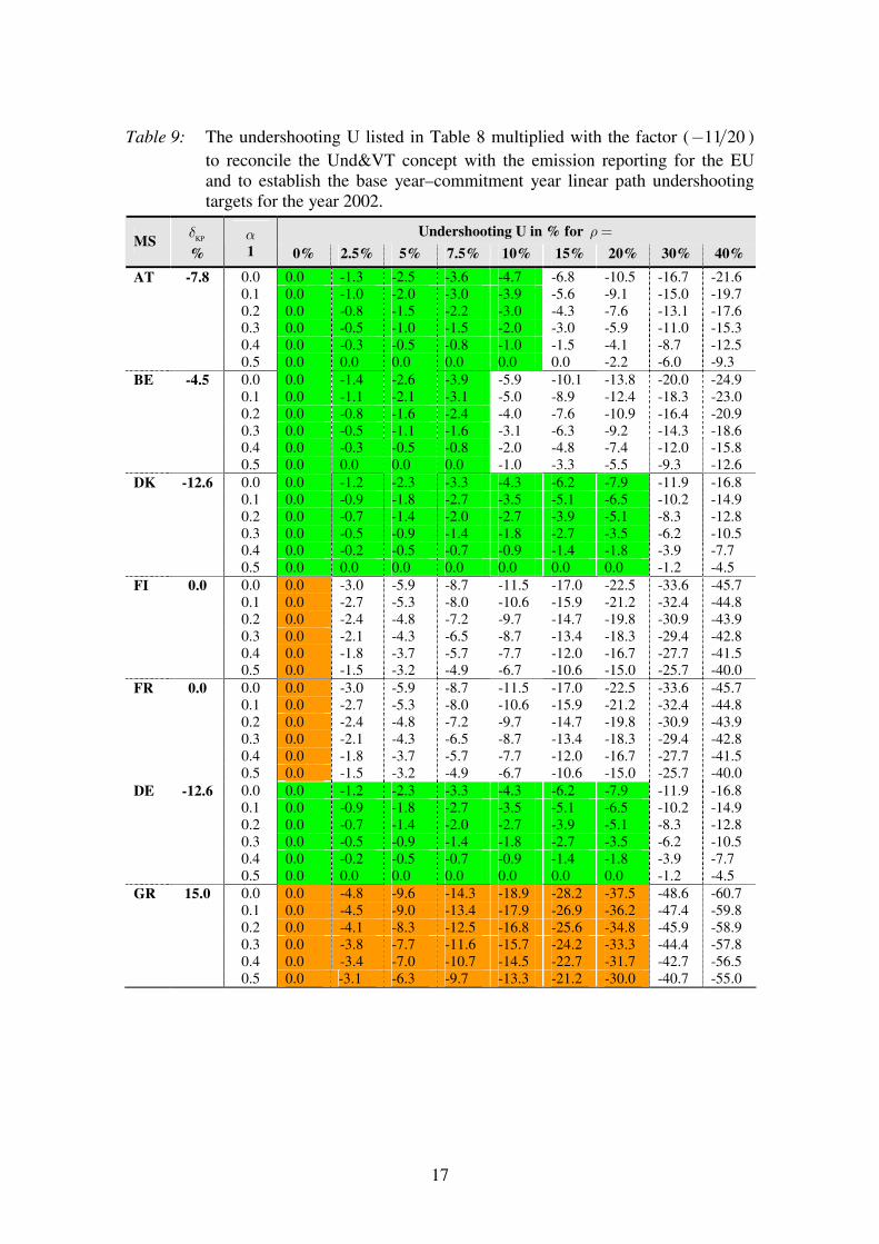
Table 9: The undershooting U listed in Table 8 multiplied with the factor ( 11 20− )
to reconcile the Und&VT concept with the emission reporting for the EU
and to establish the base year–commitment year linear path undershooting
targets for the year 2002.
Undershooting U in % for ρ = MS KP
δ
%
α
1 0% 2.5% 5% 7.5% 10% 15% 20% 30% 40%
AT -7.8 0.0 0.0 -1.3 -2.5 -3.6 -4.7 -6.8 -10.5 -16.7 -21.6
0.1 0.0 -1.0 -2.0 -3.0 -3.9 -5.6 -9.1 -15.0 -19.7
0.2 0.0 -0.8 -1.5 -2.2 -3.0 -4.3 -7.6 -13.1 -17.6
0.3 0.0 -0.5 -1.0 -1.5 -2.0 -3.0 -5.9 -11.0 -15.3
0.4 0.0 -0.3 -0.5 -0.8 -1.0 -1.5 -4.1 -8.7 -12.5
0.5 0.0 0.0 0.0 0.0 0.0 0.0 -2.2 -6.0 -9.3
BE -4.5 0.0 0.0 -1.4 -2.6 -3.9 -5.9 -10.1 -13.8 -20.0 -24.9
0.1 0.0 -1.1 -2.1 -3.1 -5.0 -8.9 -12.4 -18.3 -23.0
0.2 0.0 -0.8 -1.6 -2.4 -4.0 -7.6 -10.9 -16.4 -20.9
0.3 0.0 -0.5 -1.1 -1.6 -3.1 -6.3 -9.2 -14.3 -18.6
0.4 0.0 -0.3 -0.5 -0.8 -2.0 -4.8 -7.4 -12.0 -15.8
0.5 0.0 0.0 0.0 0.0 -1.0 -3.3 -5.5 -9.3 -12.6
DK -12.6 0.0 0.0 -1.2 -2.3 -3.3 -4.3 -6.2 -7.9 -11.9 -16.8
0.1 0.0 -0.9 -1.8 -2.7 -3.5 -5.1 -6.5 -10.2 -14.9
0.2 0.0 -0.7 -1.4 -2.0 -2.7 -3.9 -5.1 -8.3 -12.8
0.3 0.0 -0.5 -0.9 -1.4 -1.8 -2.7 -3.5 -6.2 -10.5
0.4 0.0 -0.2 -0.5 -0.7 -0.9 -1.4 -1.8 -3.9 -7.7
0.5 0.0 0.0 0.0 0.0 0.0 0.0 0.0 -1.2 -4.5
FI 0.0 0.0 0.0 -3.0 -5.9 -8.7 -11.5 -17.0 -22.5 -33.6 -45.7
0.1 0.0 -2.7 -5.3 -8.0 -10.6 -15.9 -21.2 -32.4 -44.8
0.2 0.0 -2.4 -4.8 -7.2 -9.7 -14.7 -19.8 -30.9 -43.9
0.3 0.0 -2.1 -4.3 -6.5 -8.7 -13.4 -18.3 -29.4 -42.8
0.4 0.0 -1.8 -3.7 -5.7 -7.7 -12.0 -16.7 -27.7 -41.5
0.5 0.0 -1.5 -3.2 -4.9 -6.7 -10.6 -15.0 -25.7 -40.0
FR 0.0 0.0 0.0 -3.0 -5.9 -8.7 -11.5 -17.0 -22.5 -33.6 -45.7
0.1 0.0 -2.7 -5.3 -8.0 -10.6 -15.9 -21.2 -32.4 -44.8
0.2 0.0 -2.4 -4.8 -7.2 -9.7 -14.7 -19.8 -30.9 -43.9
0.3 0.0 -2.1 -4.3 -6.5 -8.7 -13.4 -18.3 -29.4 -42.8
0.4 0.0 -1.8 -3.7 -5.7 -7.7 -12.0 -16.7 -27.7 -41.5
0.5 0.0 -1.5 -3.2 -4.9 -6.7 -10.6 -15.0 -25.7 -40.0
DE -12.6 0.0 0.0 -1.2 -2.3 -3.3 -4.3 -6.2 -7.9 -11.9 -16.8
0.1 0.0 -0.9 -1.8 -2.7 -3.5 -5.1 -6.5 -10.2 -14.9
0.2 0.0 -0.7 -1.4 -2.0 -2.7 -3.9 -5.1 -8.3 -12.8
0.3 0.0 -0.5 -0.9 -1.4 -1.8 -2.7 -3.5 -6.2 -10.5
0.4 0.0 -0.2 -0.5 -0.7 -0.9 -1.4 -1.8 -3.9 -7.7
0.5 0.0 0.0 0.0 0.0 0.0 0.0 0.0 -1.2 -4.5
GR 15.0 0.0 0.0 -4.8 -9.6 -14.3 -18.9 -28.2 -37.5 -48.6 -60.7
0.1 0.0 -4.5 -9.0 -13.4 -17.9 -26.9 -36.2 -47.4 -59.8
0.2 0.0 -4.1 -8.3 -12.5 -16.8 -25.6 -34.8 -45.9 -58.9
0.3 0.0 -3.8 -7.7 -11.6 -15.7 -24.2 -33.3 -44.4 -57.8
0.4 0.0 -3.4 -7.0 -10.7 -14.5 -22.7 -31.7 -42.7 -56.5
0.5 0.0 -3.1 -6.3 -9.7 -13.3 -21.2 -30.0 -40.7 -55.0

18
Table 9: continued.
IE 7.8 0.0 0.0 -4.7 -9.2 -13.8 -18.3 -24.8 -30.3 -41.4 -53.5
0.1 0.0 -4.3 -8.7 -13.0 -17.4 -23.7 -29.0 -40.2 -52.6
0.2 0.0 -4.0 -8.1 -12.2 -16.4 -22.5 -27.6 -38.7 -51.7
0.3 0.0 -3.7 -7.5 -11.4 -15.4 -21.2 -26.1 -37.2 -50.6
0.4 0.0 -3.4 -6.9 -10.6 -14.4 -19.8 -24.5 -35.5 -49.3
0.5 0.0 -3.1 -6.3 -9.7 -13.3 -18.4 -22.8 -33.5 -47.8
IT -3.9 0.0 0.0 -1.4 -2.7 -4.2 -6.5 -10.7 -14.4 -20.6 -25.5
0.1 0.0 -1.1 -2.2 -3.4 -5.6 -9.5 -13.0 -18.9 -23.6
0.2 0.0 -0.8 -1.6 -2.7 -4.6 -8.2 -11.5 -17.0 -21.5
0.3 0.0 -0.6 -1.1 -1.9 -3.7 -6.9 -9.8 -14.9 -19.2
0.4 0.0 -0.3 -0.6 -1.1 -2.6 -5.4 -8.0 -12.6 -16.4
0.5 0.0 0.0 0.0 -0.3 -1.6 -3.9 -6.1 -9.9 -13.2
LU -16.8 0.0 0.0 -1.1 -2.1 -3.0 -3.9 -5.6 -7.2 -10.0 -12.6
0.1 0.0 -0.8 -1.7 -2.4 -3.2 -4.6 -6.0 -8.4 -10.7
0.2 0.0 -0.6 -1.3 -1.9 -2.4 -3.6 -4.6 -6.6 -8.6
0.3 0.0 -0.4 -0.8 -1.3 -1.7 -2.4 -3.2 -4.6 -6.3
0.4 0.0 -0.2 -0.4 -0.6 -0.8 -1.3 -1.7 -2.4 -3.5
0.5 0.0 0.0 0.0 0.0 0.0 0.0 0.0 0.0 -0.3
NL -3.6 0.0 0.0 -1.4 -2.7 -4.5 -6.8 -11.0 -14.7 -20.9 -25.8
0.1 0.0 -1.1 -2.2 -3.7 -5.9 -9.8 -13.3 -19.2 -23.9
0.2 0.0 -0.8 -1.6 -3.0 -4.9 -8.5 -11.8 -17.3 -21.8
0.3 0.0 -0.6 -1.1 -2.2 -4.0 -7.2 -10.1 -15.2 -19.5
0.4 0.0 -0.3 -0.6 -1.4 -2.9 -5.7 -8.3 -12.9 -16.7
0.5 0.0 0.0 0.0 -0.6 -1.9 -4.2 -6.4 -10.2 -13.5
PT 16.2 0.0 0.0 -4.9 -9.6 -14.4 -19.0 -28.4 -37.7 -49.8 -61.9
0.1 0.0 -4.5 -9.0 -13.5 -18.0 -27.1 -36.4 -48.6 -61.0
0.2 0.0 -4.2 -8.4 -12.6 -16.9 -25.7 -35.0 -47.1 -60.1
0.3 0.0 -3.8 -7.7 -11.7 -15.8 -24.3 -33.4 -45.6 -59.0
0.4 0.0 -3.4 -7.0 -10.7 -14.6 -22.8 -31.8 -43.9 -57.7
0.5 0.0 -3.1 -6.3 -9.7 -13.3 -21.2 -30.0 -41.9 -56.2
ES 9.0 0.0 0.0 -4.7 -9.3 -13.9 -18.4 -26.0 -31.5 -42.6 -54.7
0.1 0.0 -4.4 -8.7 -13.1 -17.5 -24.9 -30.2 -41.4 -53.8
0.2 0.0 -4.1 -8.1 -12.3 -16.5 -23.7 -28.8 -39.9 -52.9
0.3 0.0 -3.7 -7.5 -11.5 -15.5 -22.4 -27.3 -38.4 -51.8
0.4 0.0 -3.4 -6.9 -10.6 -14.4 -21.0 -25.7 -36.7 -50.5
0.5 0.0 -3.1 -6.3 -9.7 -13.3 -19.6 -24.0 -34.7 -49.0
SE 2.4 0.0 0.0 -4.5 -8.3 -11.1 -13.9 -19.4 -24.9 -36.0 -48.1
0.1 0.0 -4.2 -7.7 -10.4 -13.0 -18.3 -23.6 -34.8 -47.2
0.2 0.0 -4.0 -7.2 -9.6 -12.1 -17.1 -22.2 -33.3 -46.3
0.3 0.0 -3.7 -6.7 -8.9 -11.1 -15.8 -20.7 -31.8 -45.2
0.4 0.0 -3.4 -6.1 -8.1 -10.1 -14.4 -19.1 -30.1 -43.9
0.5 0.0 -3.1 -5.6 -7.3 -9.1 -13.0 -17.4 -28.1 -42.4
UK -7.5 0.0 0.0 -1.3 -2.5 -3.7 -4.8 -7.1 -10.8 -17.0 -21.9
0.1 0.0 -1.0 -2.0 -3.0 -3.9 -5.9 -9.4 -15.3 -20.0
0.2 0.0 -0.8 -1.5 -2.3 -3.0 -4.6 -7.9 -13.4 -17.9
0.3 0.0 -0.5 -1.0 -1.5 -2.0 -3.3 -6.2 -11.3 -15.6
0.4 0.0 -0.3 -0.5 -0.8 -1.0 -1.8 -4.4 -9.0 -12.8
0.5 0.0 0.0 0.0 0.0 0.0 -0.3 -2.5 -6.3 -9.6
EC -4.8 0.0 0.0 -1.3 -2.6 -3.9 -5.6 -9.8 -13.5 -19.7 -24.6
0.1 0.0 -1.1 -2.1 -3.1 -4.7 -8.6 -12.1 -18.0 -22.7
0.2 0.0 -0.8 -1.6 -2.4 -3.7 -7.3 -10.6 -16.1 -20.6
0.3 0.0 -0.5 -1.1 -1.6 -2.8 -6.0 -8.9 -14.0 -18.3
0.4 0.0 -0.3 -0.5 -0.8 -1.7 -4.5 -7.1 -11.7 -15.5
0.5 0.0 0.0 0.0 0.0 -0.7 -3.0 -5.2 -9.0 -12.3
19
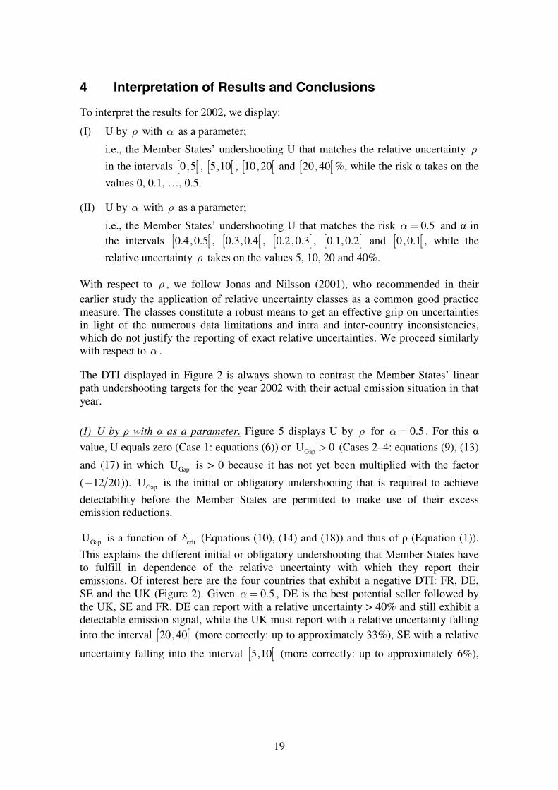
4 Interpretation of Results and Conclusions
To interpret the results for 2002, we display:
(I) U by ρ with α as a parameter;
i.e., the Member States’ undershooting U that matches the relative uncertainty ρ
in the intervals [ [0,5 , [ [5,10 , [ [10,20 and [ [20,40 %, while the risk α takes on the
values 0, 0.1, …, 0.5.
(II) U by α with ρ as a parameter;
i.e., the Member States’ undershooting U that matches the risk 0.5α= and α in
the intervals [ [0.4,0.5 , [ [0.3,0.4 , [ [0.2,0.3 , [ [0.1,0.2 and [ [0,0.1 , while the
relative uncertainty ρ takes on the values 5, 10, 20 and 40%.
With respect to ρ , we follow Jonas and Nilsson (2001), who recommended in their
earlier study the application of relative uncertainty classes as a common good practice
measure. The classes constitute a robust means to get an effective grip on uncertainties
in light of the numerous data limitations and intra and inter-country inconsistencies,
which do not justify the reporting of exact relative uncertainties. We proceed similarly
with respect to α .
The DTI displayed in Figure 2 is always shown to contrast the Member States’ linear
path undershooting targets for the year 2002 with their actual emission situation in that
year.
(I) U by ρ with α as a parameter. Figure 5 displays U by ρ for 0.5α= . For this α
value, U equals zero (Case 1: equations (6)) or GapU 0> (Cases 2–4: equations (9), (13)
and (17) in which GapU is > 0 because it has not yet been multiplied with the factor
( 12 20− )). GapU is the initial or obligatory undershooting that is required to achieve
detectability before the Member States are permitted to make use of their excess
emission reductions.
GapU is a function of critδ (Equations (10), (14) and (18)) and thus of ρ (Equation (1)).
This explains the different initial or obligatory undershooting that Member States have
to fulfill in dependence of the relative uncertainty with which they report their
emissions. Of interest here are the four countries that exhibit a negative DTI: FR, DE,
SE and the UK (Figure 2). Given 0.5α= , DE is the best potential seller followed by
the UK, SE and FR. DE can report with a relative uncertainty > 40% and still exhibit a
detectable emission signal, while the UK must report with a relative uncertainty falling
into the interval [ [20,40 (more correctly: up to approximately 33%), SE with a relative
uncertainty falling into the interval [ [5,10 (more correctly: up to approximately 6%),

20
and FR even with a relative uncertainty falling into the interval [ [0,5 % (more correctly:
up to approximately 3%), respectively.7
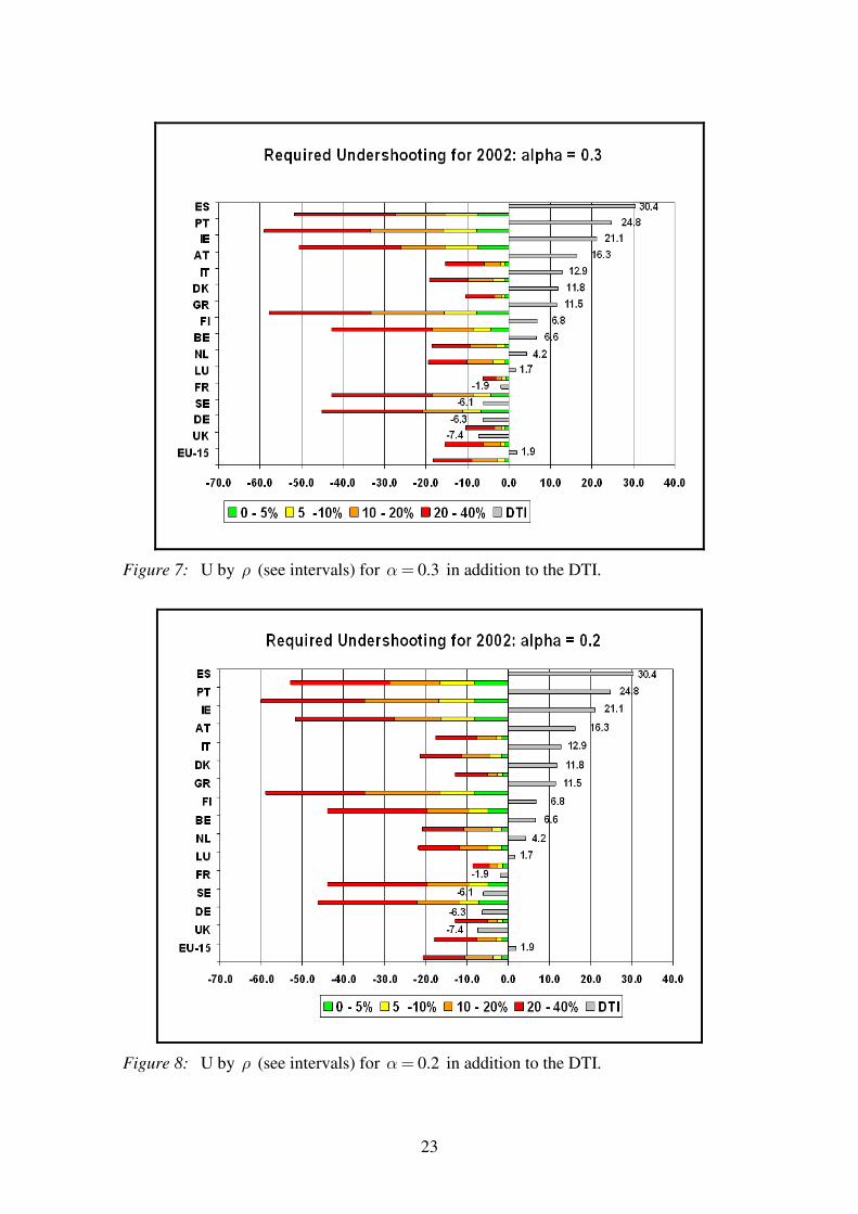
Figures 6–10 display U by ρ for 0.4,...,0.0α= . These figures can be interpreted
similarly to Figure 5, bearing in mind that U increases in absolute terms with decreasing
α . For 0.0α= , DE and the UK must report with a relative uncertainty falling into the
interval [ [10,20 (more correctly: up to approximately 15%), and both SE and FR even
with a relative uncertainty falling into the interval [ [0,5 % (more correctly: up to
approximately 3% and 2%, respectively).8
(II) U by a with ρ as a parameter. Figure 11 displays U by α for 5%ρ= . For this ρ
value, a white bar or, equivalently, a GapU 0< (i.e., > 0 if the factor ( 12 20− ) is
disregarded) appears only for Member States committed to emission limitation (ES, FI,
FR, GR, IE, PT and SE; see Table 1). A GapU 0< satisfies our demand for detectable
signals. As it becomes obvious, the white bars represent the major part of U. Their
length is equivalent to the length of the green bars in Figure 5.
With increasing ρ (Figures 12–14), an increasing number of Member States committed
to emission reduction also exhibit a GapU 0< , for 40%=ρ eventually all of them
(Figure 14). For 10%ρ= , the length of the white bars is equivalent to the combined
length of the green and yellow bars in Figure 5; and so on until Figure 14 ( 40%ρ= ),
where the length of the white bars is equivalent to the combined length of the green,
yellow, orange and red bars in Figure 5. Figures 12–14 still resolve GapU better than the
remainder of U.
We prefer interpretation I (U by ρ with α as a parameter; Figures 5–10) over
interpretation II (U by α with ρ as a parameter; Figures 11–14), as the use of α
instead of ρ as a parameter appears to be more readily acceptable. Nevertheless,
Figures 11–14 are well suited to quickly survey GapU and analyze which Member State
with a negative DTI meets GapU for a given ρ . (SE, e.g., meets GapU for 5%ρ= but
not any more for 10%ρ= ; Figures 11 and 12.)
The following four conclusions emerge from our exercise:
(1) Jonas et al. (2004a) motivated the application of preparatory signal detection in the
context of the Kyoto Protocol as a necessary measure that should have been taken
prior to/in negotiating the Protocol. To these ends, the authors have applied four
7 The exact values are derived by demanding that
GapU (as given by equation (10) for the UK and
equation (14) for FR and SE) equals a Member State’s DTI (multiplied with ( )20 12− ) and resolving the
resulting equation for the relative uncertainty ρ .
8 The exact values are derived by demanding that a Member State’s DTI (multiplied with ( )20 12− ) is
reproduced by using equation (6) for DE, (9) for the UK, (13) for FR and (17) for SE, respectively.

21
preparatory signal detection techniques to the Annex I countries under the Kyoto
Protocol. The frame of reference for preparatory signal detection is that Annex I
countries comply with their committed emission targets in 2008–2012. By contrast,
in this study we apply one of these techniques, the Und&VT concept, to the Member
States of the European Union under the EU burden sharing in compliance with the
Kyoto Protocol, but with reference to the base year–commitment year linear path
undershooting targets in 2002. Thus, our exercise shows that preparatory signal
detection can also be applied in connection with interim emission targets.
(2) To advance the reporting of the EU we take, in addition to the DTI, uncertainty and
its consequences into consideration, i.e., we determine (i) the risk that a Member
State’s true emissions in the commitment year/period are above its true EU
reference line; and (ii) the detectability of its target. We anticipate that the
evaluation of emission signals in terms of risk and detectability will become
standard practice and that these two qualifiers will be accounted for in pricing GHG
emission permits.
(3) In 2002 only four Member States exhibit a negative DTI and thus appear as potential
sellers: DE, FR, SE and the UK (Figure 2). However, expecting that the EU Member
States exhibit relative uncertainties in the range of 5–10% and above rather than
below, excluding emissions/removals due to LUCF (Table 2), the Member States
require considerable undershooting of their EU-compatible, but detectable, targets if
one wants to keep the risk low ( 0.1α≈ ) that the Member States’ true emissions in
the commitment year/period are above their true EU reference lines. These
conditions can only be met by two Member States, DE and the UK (ranked in terms
of creditability) (Figure 9). SE and FR can only act as potential high-risk sellers, SE
within the 5–10% relative uncertainty class and FR within the 0–5% relative
uncertainty class (Figure 5).
(4) The Und&VT concept requires detectable signals. Measuring emission reductions
negatively and emission increases positively (i.e., in line with the reporting for the
EU), it can be stated that the greater the committed emission limitation or reduction
targets KPδ and the greater the relative uncertainty ρ, with which Member States
report their emissions, the smaller the initial or obligatory undershooting GapU is to
achieve detectability. That is, for 5%ρ= only the Member States committed to
emission limitation (ES, FI, FR, GR, IE, PT and SE) require a GapU 0< . For these
Member States, GapU represents the major part of the undershooting U (Figure 11).
For 10%ρ= , BE, IT, the NL as well as the EU (EU-15) as a whole also require a
GapU 0< (Figure 12), indicating that somewhere within the 5–10% relative
uncertainty range non-detectability will become a problem also for these Member
States as well as the EU. The maximal (critical) relative uncertainties, with which
they can report their emissions without compromising detectability, can be
determined (Jonas et al., 2004a:Section 3.1); these are 8.1% (BE), 7.0% (IT), 6.4%
(NL) and 8.7% (EU-15), respectively, assuming that the emission limitation or
reduction targets are met under the EU burden sharing in compliance with the Kyoto
Protocol. From these numbers it becomes clear that the negotiations for the Kyoto
Protocol were imprudent because they did not consider the consequences of
uncertainty.

22
Figure 5: U by ρ (see intervals) for 0.5α= in addition to the DTI.
Figure 6: U by ρ (see intervals) for 0.4α= in addition to the DTI.
23
Figure 7: U by ρ (see intervals) for 0.3α= in addition to the DTI.
Figure 8: U by ρ (see intervals) for 0.2α= in addition to the DTI.

24
Figure 9: U by ρ (see intervals) for 0.1α= in addition to the DTI.
Figure 10: U by ρ (see intervals) for 0.0α= in addition to the DTI.

25
Figure 11: U by α (see value and intervals) for 5%ρ= in addition to the DTI.
Figure 12: U by α (see value and intervals) for 10%ρ= in addition to the DTI.

26
Figure 13: U by α (see value and intervals) for 20%ρ= in addition to the DTI.
Figure 14: U by α (see value and intervals) for 40%ρ= in addition to the DTI.

27
References
EEA (2003). EU greenhouse gas emissions rise for second year running. News Release,
6 May, European Environment Agency (EEA), Copenhagen, Denmark. Available
at: http://org.eea.eu.int/documents/newsreleases/ghg-2003-en.
EEA (2004). EU greenhouse gas emissions decline after two years of increases. News
Release, 15 July, European Environment Agency (EEA), Copenhagen, Denmark.
Available at: http://org.eea.eu.int/documents/newsreleases/tec2-2004-en.
Gugele, B., K. Huttunen, M. Ritter and M. Gager (2004). Annual European Community
Greenhouse Gas Inventory 1990–2002 and Inventory Report 2004. Technical
Report No. 2, European Environment Agency (EEA), Copenhagen, Denmark, pp.
177. Available at: http://reports.eea.eu.int/technical_report_2004_2/en.
IPCC (1997a,b,c). Revised 1996 IPCC Guidelines for National Greenhouse Gas
Inventories, Volume 1: Greenhouse Gas Inventory Reporting Instructions;
Volume 2: Greenhouse Gas Inventory Workbook; Volume 3: Greenhouse Gas
Inventory Reference Manual. Intergovernmental Panel on Climate Change (IPCC)
Working Group I (WG I) Technical Support Unit, IPCC/OECD/IEA, Bracknell,
United Kingdom. Available at: http://www.ipcc-nggip.iges.or.jp/public/gl/invs1.
htm.
Jonas, M. and S. Nilsson (2001). The Austrian Carbon Database (ACDb) Study ―
Overview. Interim Report IR-01-064. International Institute for Applied Systems
Analysis, Laxenburg, Austria, pp. 131. Available at: http://www.iiasa.ac.at/
Research/FOR/acdb.html.
Jonas, M., S. Nilsson, R. Bun, V. Dachuk, M. Gusti, J. Horabik, W. Jęda and Z.
Nahorski (2004a). Preparatory Signal Detection for Annex I Countries under the
Kyoto Protocol ― A Lesson for the Post-Kyoto Policy Process. Interim Report
IR-04-024. International Institute for Applied Systems Analysis, Laxenburg,
Austria, pp. 91. Available at: http://www.iiasa.ac.at/Publications/Documents/IR-
04-024.pdf.
Jonas, M., S. Nilsson, R. Bun, V. Dachuk, M. Gusti, J. Horabik, W. Jęda and Z.
Nahorski (2004b). Preparatory Signal Detection for the EU Member States Under
EU Burden Sharing ― Advanced Monitoring Including Uncertainty (1990–2001).
Interim Report IR-04-029. International Institute for Applied Systems Analysis,
Laxenburg, Austria, pp. 91. Available at: http://www.iiasa.ac.at/Publications/
Documents/IR-04-029.pdf.
Penman, J., D. Kruger, I. Galbally, T. Hiraishi, B. Nyenzi, S. Emmanuel, L. Buendia, R.
Hoppaus, T. Martinsen, J. Meijer, K. Miwa and K. Tanabe (eds.) (2000). Good
Practice Guidance and Uncertainty Management in National Greenhouse Gas
Inventories. Institute for Global Environmental Strategies, Hayama, Kanagawa,
Japan. Available at: http://www.ipcc-nggip.iges.or.jp/public/gp/gpgaum.htm.

28
Acronyms and Nomenclature
EU European Union
DTI Distance-to-Target Indicator
GHG Greenhouse Gas
KP Kyoto Protocol
LUCF Land-use Change and Forestry
MS Member State
Und Undershooting
Und&VT Undershooting and Verification Time
VT Verification Time
crit critical
mod modified
t true

29
ISO Country Code
AT Austria
BE Belgium
DE Germany
DK Denmark
EC European Community
ES Spain
FI Finland
FR France
GR Greece
IE Ireland
IT Italy
LU Luxembourg
NL Netherlands
PT Portugal
SE Sweden
UK United Kingdom