Preliminary,comments welcome

INFLATIONAND FINANCIAL SECTOR SIZE*

William B. English

Federal Reserve Board20th and C Streets, NWWashington,DC 20551

May 1991

Revised: April 1996

ABSTRACT

Traditionallythe cost of expected inflation has been seen as the“shoeleathercost” of going to the bank more often. This paperfocuses on the other side of these transactions--i.e., on theincreased production of financial services by financial firms. Iconstruct a model in which households must make purchases either withcash or with costly transactionsservices produced by firms in thefinancial services sector. One can think of these services as beingthe use of a credit card or other method of paying without cash. Inthe model, a higher inflation rate leads households to substitutepurchased transactions services for money balances. As a result, thefinancial services sector gets larger. A test of the model usingcross-sectionaldata finds that the size of a nation’s financialsector is strongly affected by its inflation rate. The empiricalresults provide an alternativeway to measure the costs of inflation.These costs appear to be large.

JEL Classification:E31

*The analysis and conclusion in this paper are mine alone and do notindicate &oncurrence by other members-of the research staffs, by theBoard of Governors, or by the Federal Reserve Banks. I thank seminarparticipantsat the University of Pennsylvania,the University ofMaryland, Johns Hopkins University, and the Federal Reserve Board foruseful comments on earlier drafts of this paper. Mauricio Fernholzprovided excellent research assistance. All-remainingerrors aremine.

-2-

Introduction

Traditionally,the cost of expected inflation has been viewed

primarily as the “shoeleathercost” of going to the bank more often,

as in the familiar Baumol-Tobinparable (Baumol,1952; Tobin, 1956).

In this view, households reduce their average holdings of cash by

making smaller withdrawals with greater frequency, and the cost of the

inflation is the utility loss associatedwith trips to the bank,

waiting in line, etc. This paper focuses on the banks’ side of these

transactions:in order to satisfy the increased customer activity,

banks may need to hire additional tellers, build more and larger

branches, or make other costly investmentsin automation or

technology. Thus, the cost of inflation can be viewed, at least in

part, as the result of resources transferredto the financial sector

to accommodatethe increased number of transactionschosen by

households as they attempt to shift the cost of holding currency onto

others. These resources are a social loss because if inflationwere

lower, the resources could be used directly to increase production of

consumer goods.

This focus on the effects of inflation on the size of the

financial sector is not new. Bresciani-Turroni, in his history of the

German hyperinflation,notes that inflation caused a ‘hypertrophyof

the banking system~ in late 1922 and 1923 (Bresciani-Turroni, 1937, p.

215). For example he reports that more than 400 new banks were

established.in1923, the peak year of the hyperinflation. This was

more than four times the number establishedin 1922, and six times the

number established in 1920 and 1921. At the same time, existing banks

were extending their branch networks and greatly increasing their

employment. There were 30,489 employees at the ‘DV banks (Deutsche

-3-

Bank, Diskonto-Gesellschaft, DarmstadterBank, and Dresdner Bank) in

1920. By 1922 there were more than 45,000 employees, and by the fall

of 1923, when the inflationwas at its peak, almost 60,000.

Bresciani-Turroninotes that the increase in banking activity

reflected a higher volume of financial transactions rather than an

increase in real activity. Indeed, the number of current accounts at

the three largest “D” banks rose from less than 1.5 million at the end

of 1920 to an estimated 2.5 million at the end of 1923.

The rapid expansion in the banking sector generatedby the

German hyperinflationreversed sharply following stabilization. The

number of new banks establishedfell by more than 80 percent in 1924,

to just 74. The number of employees at the four ‘Dn banks declined by

nearly a half by the end of 1924, and the number of current accounts

at the three largest “D” banks fell by three-quartersover the same

period, A similar pattern of decline in the size of the financial

sector following stabilizationwas noted by Weber (1986)in his study

of the ends of hyperinflationsin Eastern Europe in the 1920s. He

cites one estimate that 4,000 of 12,000 bank officials in Budapest

became unemployed following the stabilizationin Hungary, and he

estimates that 10,000 bank employees lost their jobs following the

Austrian stabilization.

In order to address this issue, I construct a model in which

households can make purchaseswith cash or with purchased transactions

services. A number of recent papers (e.g. Cole and Stockman, 1992;

Schreft, 1992; Gillman, 1993; Dotsey and Ireland, 1993) present models

in which households can transact without money at some cost in terms

of labor. While these models allow for alternativemethods of

transacting,the focus on labor costs seems to capture primarily the

cost of household “home production” of financial services. In

-4-

contrast, the approach taken here is to allow agents to make purchases

with “transactionsservices~ supplied by banks or other financial

firms as in Fischer (1983),Prescott (1987),and Aiyagari et al.

(1995). In the model, households are constrainedto make purchases

1either with cash or with purchased transactionsservices. One can

think of these services as interest-bearingchecking accounts, money

market mutual funds, overdraft services, or credit cards. An increase

in the inflation rate induces households to substitute transactions

services for real balances. As a result, increases in the inflation

rate increase the size of the financial sector.

I test this implicationof the model using cross-sectional

data on financial sector size and inflation rates. The results

suggest that the effect of inflation on the size of the financial

sector is significantboth economicallyand statistically. The

empirical model indicates that the effect of a 10 percent inflation in

the United States would be to increase the share of GDP produced in

the financial sector by almost 1-1/2 percentage points. This estimate

of the cost of inflation is larger than those found in earlier

studies, such as those of Fischer (1981) and Lucas (1981),although it

is similar to that found in a recent study by Lucas (1994).

I. The Model

The economy contains a continuum of identical agents, indexed

by ic[O,l], each with infinite horizons. Each period they supply a

1. One could also require firms to transact with cash ortransactions services. This issue is discussed below. In practice,firms’ purchases of cash management services are likely veryimportant.

-5- :

2unit of labor inelasticallyand receive a wage, w. They hold two

assets: capital and money. Each period the capital is rented to firms

at a rental rate r. Agents must purchase their consumptionfor the

period using their start-of-periodmoney balances or by purchasing

transactions services. One could motivate this constraintby assuming

that households include two individual agents, one of which works

while the other shops (see, for example, Lucas and S-tokey, 1987). At

the end of the period, households receive their wage and a cash

transfer from the government,and they pay for the purchases made

with transactionsservices as well as for the services themselves.

Then they choose their money and capital holdings for the start of the

next period, and the period ends.

The economy has three types of firms. Firms in the

consumption goods sector produce one of a continuum of consumption

goods. The market for each of the goods is competitive. Firms in the

capital goods sector produce capital. Firms in the transactions

services sector produce transactionsservices. As discussed below,

capital and transactionsservices can be purchasedwithout cash or

transactions services. Firms in all three sectors are competitive,

and production in each sector requiresboth capital and labor.

A. The TransactionsTechnology

There is a continuum of goods in the economy indexed by j,

je[O,l]. Each good is assumed to be purchasedwith a separate

transaction. Agents can pay cash, or incur a fixed cost, q, to make

the purchase without cash. Because the cost of making a purchase

2. If labor supply were not inelastic,then inflationwould affectlabor supply. Since my focus here is on the effects of inflation onthe size of the financial sector, I do not take account of thispossible effect. See Aiyagari et al. (1995) for a related model thatincludes an effect of inflation on labor supply.

-6-

without money is independentof the size of the transaction,agents

will make small transactionswith cash and large ones with

transactions services. This approach is similar to that taken by

Whitesell (1989, 1992) in studies of the optimal use of alternatives

to cash purchases, although Whitesell (1992) allows for more than one

alternativeto cash and both a fixed and a proportionalcost of

transactingwithout cash.

Other recent models take a variety of approaches to get a

margin along which agents adjust to reduce cash transactionsin the

face of higher inflation. In Gillman (1993) and Aiyagari et al.

(1995)the cost of making a purchase without cash is assumed to be

proportionalto the size of the transaction,and the size of the cost

differs exogenouslyacross goods. In Schreft (1992)and Dotsey and

Ireland (1993),the cost is assumed to be larger for goods purchased

farther from the agent’s location on a unit circle.

The cost structure assumed here has the intuitivelyappealing

implicationthat cash transactionstend to be smaller than check or

credit purchases. Evidence on actual household transactionscan be

obtained from the preliminary results of the 1995 Survey of Consumer

TransactionsAccounts Usage, commissionedby the Board of Governors of

the Federal Reserve System and conducted by the University of Michigan

Survey Research Center. This survey, conducted in May 1995, showed

that the mean size of household check transactionswas $80, the mean

size of credit card purchaseswas $54, and the mean size of debit card

transactionswas $24. By contrast, the mean cash purchase was $11.

The pattern of transactions sizes is similar to the one prevailing in

the mid-1980s, as reported by Whitesell (1992). The 1995 survey

showed that on average households used checks to make 15 purchases a

month, credit cards to make 4 purchases, debit cards to make 1

“p-

urchase, and cash to make 29 purchases. Thus, cash was used for

nearly 60 percent of purchases,but those purchases accounted for

less than 20 percent of the dollar volume of expenditures.

The nature of the cost of transactingwithout cash differs

across the papers in this area. Gillman (1993),Dotsey and Ireland

(1993),and Schreft (1992) all assume that the cost is a labor cost--

perhaps focusing on the purchaser’snuisance costs of writing a check,

keeping records, waiting while the store verifies the check, etc. By

contrast, this paper, like Prescott (1987) and Aiyagari et al. (1995),

focuses on the production of transactionsservices by financial firms.

The model in Fischer (1983)allows for both household production of

transactions services and purchases of transactionsservices from

banks, with their marginal costs equalized in equilibrium. Whitesell

(1989) suggests a number of types of costs, including nuisance costs,

seller charges, and bank charges, but his model does not focus on the

production of transactions services or their welfare implications. It

would be straightforwardto add to the model an additional nuisance

cost of using transactions services. Doing so would clearly raise the

welfare cost of inflation,but would not greatly change the results of

the model.3

In the model presented here agents pay a fixed cost for

transaction services. In practice, of course, the purchaser generally

does not actually pay the fixed cost of the transaction. While some

banks do have per-check fees on some accounts, and some sellers have

different prices for cash and credit purchases, these direct payments

3. The nuisance costs could even be negative, especially for largetransactions,owing to the possibilitythat large amounts of cashcould be lost or stolen.

-8-

4are the exception. More commonly, the costs of transacting

without cash are implicit--feesand lower interest rates paid on

checkable accounts, for example. In addition, decisions made by

retailers,who absorb a part of the transactionscost, likely generate

effects much like those of a fixed cost. For example, some stores

have a minimum size for credit card purchases. Alternatively,stores

selling products that generally yield small transaction sizes (e.g.,

newsstands or coffee shops) are presumably less likely to accept

checks or credit cards because the associated costs would require too

large a percentage increase in prices.

The assumption that the cost of transactingwithout cash is

independent of transaction size may not be strictly true for very

large transactions,but it seems more reasonablethan the assumption

that the cost is proportionalto the transaction size. The cost of

clearing a personal check through the payments system, for example, is

likely the same virtually regardlessof the amount of the purchase.

For example, the Federal Reserve System’s functional cost analysis

reports a fixed estimated cost for individual check transactions

regardless of size (FederalReserve System, 1995). The same should be

true for credit card transactions. For retailers,the costs of

verifying checks and credit card accounts as well as the subsequent

paperwork should not depend on the size of the transaction (although

retailersmay be more likely to verify large transactions). As for

purchasers,the nuisance costs of writing the check or waiting for the

clerk to handle the transactionare likely very similar for widely

different transaction sizes.

4. Of course, a higher credit price would amount to a proportional,rather than a fixed, cost of transactingwithout cash (see Aiyagari etal., 1995, p. 9).

-9-

1 assume that capital goods can be purchasedwithout cash at

5no cost. Not doing so would generate an investment distortion as

in Stockman (1981). Aiyagari et al. (1995) assume that households

augment their capital holdings by purchasing equal amounts of each

consumption good. As a result, capital is purchased in part with cash

and in part with transactions services. Purchases of capital are

likely very large, however, compared to the average household

purchase. For example, the average size of a check purchase,

including purchases by businesses, is about $1150, while the average

size for households, as noted above, is only $80 (Humphrey,et al.,

1995). Thus the assumption in Aiyagari et al. may greatly

overestimatethe cash portion of capital purchases. One could model

purchases of capital in a manner similar to that used for consumption

goods here--allowingthe size distributionof capital goods purchases

to differ from that for consumption goods. Implicitly,I am assuming

that capital goods purchases are so large that they can be made

without cash at negligible cost.

B. The Household’s Problem

The representativehousehold gets utility in a given period

based on consumptionof the various consumptiongoods:

1 @(j)cjl-yu= J dj

o l-y

where c .Jis the consumptionof good j, y is the inverse of the

intertemporalelasticity of substitution,and ~(j) is a weighting

function. I assume that ~(j) is increasing in j, and that ~(l) is

5. I also assume that firms do not need to pay cash in advance forlabor and capital services.

-1o-

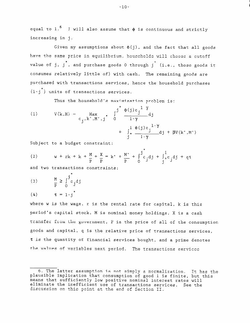
6equal to 1. I will also assume that ~ is continuous and strictly

increasing in j.

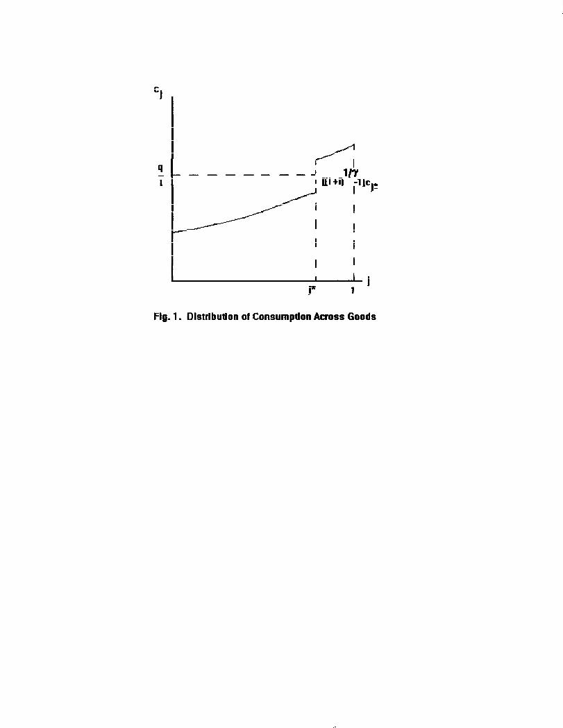
Given my assumptionsabout ~(j), and the fact that all goods

have the same price in equilibrium,households will choose a cutoff*

value of j, j , and purchase goods O through j* (i.e.,those goods it

consumes relatively little of) with cash. The remaining goods are

purchasedwith transactions services,hence the household purchases

(1-j’) units of transactions services.

Thus the household’smaximization problem is:

(1) V(k,M) = Max Jj* ~(j)cjl-y

dj.,k’,M’,j* O

CJl-y

1 $(j)cj l-y+ J dj + ~V(k’,M’)j* l-y

Subject to a budget constraint:*

(2)j 1w+rk+k+~+ ? =k’ +“’ + ~ c.dj + ~*cjdj + qt

PP ‘OJjPand two transactionsconstraints:

(3)

*(4) ~= l-j

where w is the wage, r is the rental rate for capital, k is this

period’s capital stock, M is nominal money holdings, X is a cash

transfer from the government,P is the price of all of the consumption

goods and capital, q is the relative price of transactions services,

T is the quantity of financial services bought, and a prime denotes

the values of variables next period. The transactionsservices

6. The latter assumption is not simply a normalization. It has theplausible implicationthat consumptionof good 1 is finite, but thismeans that sufficientlylow positive nominal interest rates willeliminate the inefficientuse of transactionsservices. See thediscussion on this point at the end of Section II.

-11-

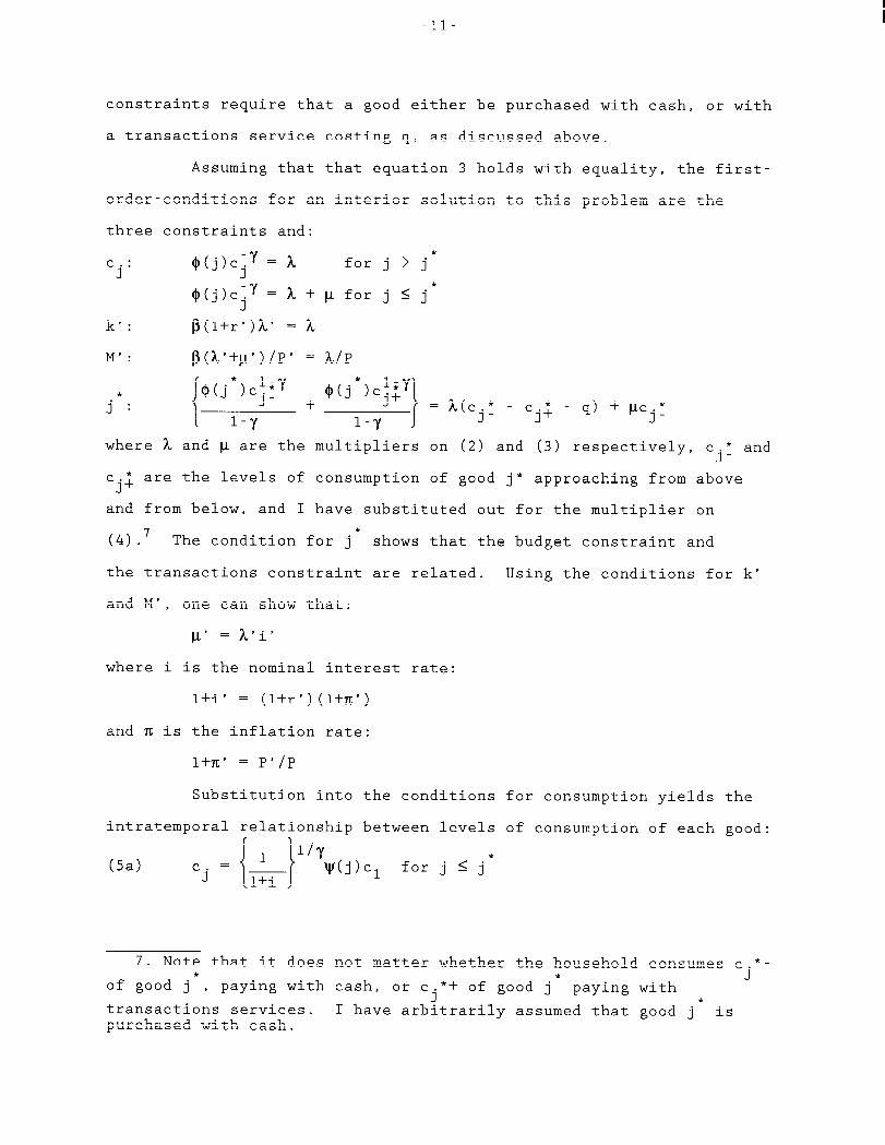
constraints require that a good either be purchasedwith cash, or with

a transactionsservice costing q, as discussed above,

Assuming that that equation 3 holds with equality, the first-

order-conditionsfor an interior solution to this problem are the

three constraintsand:

Cj: O(j)c:y = ~ for j > j*J

@(j)c~Y=L+pfor j <j’

M’: P(L’+P’)/p’ = ~,p

where ~ and p are the multipliers on (2) and (3) respectively,c.* andJ-

* are the levels of consumption of good j* approachingfrom aboveCj+and from below, and I have substitutedout for the multiplier on

(4).7 The condition for j* shows that the budget constraint and

the transactionsconstraint are related. Using the conditions for k’

and M’, one can show that:

P’ =~’i’

where i is the nominal interest rate:

l+i’ = (l+r’)(l+m’)

and n is the inflation rate:

1+~’ = P’/P

Substitutioninto the conditions for consumptionyields the

intratemporalrelationshipbetween levels of consumptionof each good:

{1

1 lly(5a) ~(j)cl for j <j’Cj = l+i

7. Note that it does not matter whether the household consumes c.*-* J

of good j , paying with cash, or c+’+ of good j* paying with*

transactionsservices. I have arbitrarilyassumed that good j ispurchased with cash.

-12-

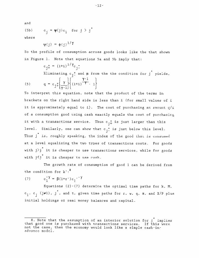
and

(5b) Cj = ~(j) Cl for j > j*

where

So the profile of consumptionacross goods looks like the that shown

in Figure 1. Note that equations 5a and 5b imply that:

Cj$= (l+i)l/yC .j-

(5)

Eliminating c .**

and p from the the condition for j yields,

q=cj${filf~+i)y- 1}To interpret this equation, note that the product of the terms in

brackets on the right hand side is less than i (for small values of i

it is approximatelyequal to i). The cost of purchasing an amount q/i

of a consumption good using cash exactly equals the cost of purchasing

it with a transactions service. Thus C .*J+

is just larger than this

level. Similarly, one can show that c.* is just below this level.J-

*

Thus j is, roughly speaking, the index of the good that is consumed

at a level equalizing the two types of transactionscosts. For goods

with j>j’ it is cheaper to use transactionsservices,while for goods*

with j<j it is cheaper to use cash.

The growth rate of consumptionof good 1 can be derived from

the condition for k’:8

(7) ‘y = ~(l+r’ )c ~“Yc1 1

Equations (2)-(7)determine the optimal time paths for k, M,

cl’ Cj(j#l), j*, and ~, given time paths for r, w, q, n, and X/P plUS

initial holdings of real money balances and capital.

8. Note that the assumption of an interior solution for j* impliesthat good one is purchasedwith transactionsservices. If this werenot the case, then the economy would look like a simple cash-in-advance model.

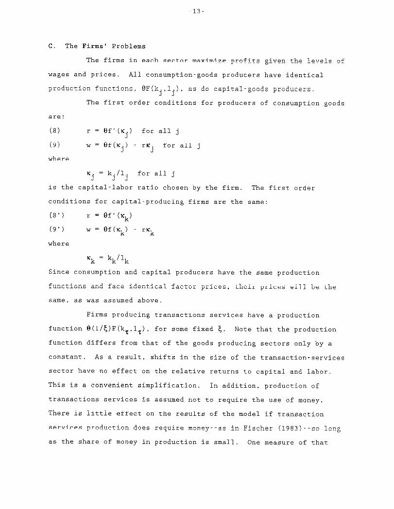
c. The Firms’ Problems

The firms in each sector maximize profits given the levels of

-13-

wages and prices. All consumption-goodsproducers have identical

production functions, eF(kj,lj), as do capital-goodsproducers.

The first order conditions for producers of consumption goods

are:

(8) r = Of’(Kj) for all j

(9) w = 9f(Kj) - rKj for all j

where

= k./l.‘j J J

for all j

is the capital-laborratio chosen by the firm. The first order

conditions for capital-producingfirms are the same:

(8’) r = ef’(Kk)

(9’) w = 6f(Kk) - rKk

where

‘k = kk/lk

Since consumptionand capital producers have the same production

functions and face identical factor prices, their prices will be the

same, as was assumed above.

Firms producing transactionsservices have a production

function e(l/~)F(kz,lz),for some fixed ~. Note that the production

function differs from that of the goods producing sectors only by a

constant. As a result, shifts in the size of the transaction-services

sector have no effect on the relative returns to capital and labor.

This is a convenient simplification. In addition, production of

transactions services is assumed not to require the use of money.

There is little effect on the results of the model if transaction

services production does require money--as in Fischer (1983)--solong

as the share of money in production is small. One measure of that

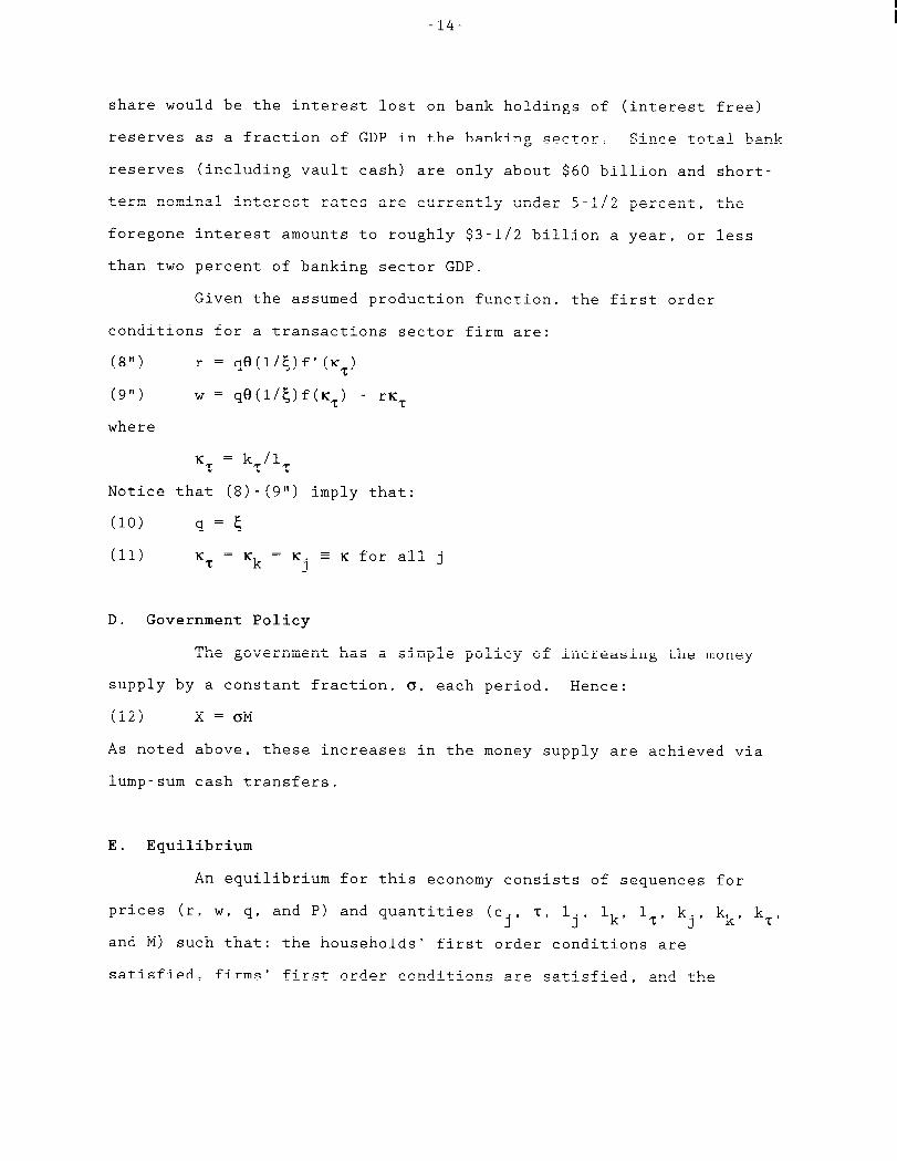
-14-

share would be the interest lost on bank holdings of (interestfree)

reserves as a fraction of GDP in the banking sector. Since total bank

reserves (includingvault cash) are only about $60 billion and short-

term nominal interest rates are currently under 5-1/2 percent, the

foregone interest amounts to roughly $3-1/2 billion a year, or less

than two percent of banking sector GDP.

Given the assumed production function, the first order

conditions for a transactions sector firm are:

(8U) r = qe(l/~)f’(K~)

(9”) w = qe(l/&)f(Kz) - rKt

where

Notice that (8)-(9”)imply that:

(lo) q=g

(11) K =T ‘k = = K for all j

‘j –

D. Government Policy

The governmenthas a simple policy of increasing the money

supply by a constant fraction, a, each period. Hence:

(12) X = GM

As noted above, these increases in the money supply are achieved via

lump-sum cash transfers.

E. Equilibrium

An equilibriumfor this economy consists of sequences for

prices (r, w, q, and P) and quantities (c., z, 1., lk, lt, k., k ,J J J kk z’

and M) such that: the households’ first order conditions are

satisfied,firms’ first order conditions are satisfied, and the

-15-

markets for each of the consumption goods, money, transactions

services, capital, and labor clear.

Market clearing in the consumptiongoods markets is:

(13) = eljf(K) for all jCj

Market clearing in the transactionssector is given by:

(14) l-j* = 6(1/~)l~f(K)

Market clearing in the money market is:

(15) M’ = (l+o)M

Market clearing in the rental market for capital is:

(16) ~lkjdj + kk + k = ko T

and market clearing in the purchase market for capital is:

(17) k’ - k = elkf(K)

Market clearing in the labor market is:

(18)

Because of Walras’ law, one of the market clearing conditionswill be

redundant.

F. Steady-stateConditions

In the steady state equations (2)-(7), (8)-(12),and (13)-

(18) will hold with constant values of c., j*, T, K, M/p, Ik, I IJ T’ j’

‘k’ ‘I’ ‘j’ “ “ “ and q“ Let these constant values be indicatedby

bars, =. , etc.JMarket clearing in the money market, equation 15, implies

that:

The first-order condition for consumptionof good 1, equation

7, implies that in steady state the marginal product of capital must

equal the rate of time preference:

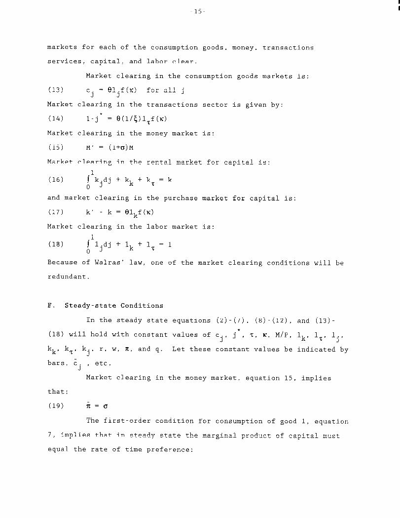
-16-

(20) ef’(i) = swhere

K = kll

Equation (20) yields the steady-statecapital stock. Note

that it is not affected by the level of inflation. The economy is not

super-neutral,however, because a change in ~ will affect ~., ~*,J

and

m.

Substitutioninto the household’sbudget constraint,equation

2, yields the feasibilitycondition:

(21)

which shows that total output must be equal to total consumptionof

the various consumption goods plus purchases of financial services.

In steady state, the relative consumption of the various

goods can be obtained from equations 5a and 5b:

‘22a)‘j={(l+3);l+a,}1’y~(j):l ‘orjsj*and

(22b) ‘.CJ

= ~(j)=1 for j > j**

The steady state condition for j is given by:

{ }{(23) - * ‘Y

y-1

Cj+ v }((1+5) (1+0) )~- 1 = ~

The steady-state levels of ~~ and ~* are jointly determinedby (21)

and (23), after substitutingfor the c.‘s using (22a) and (22b). ThenJ

the steady-state levels of the c.J‘s can be obtained from (22a) and

(22b).

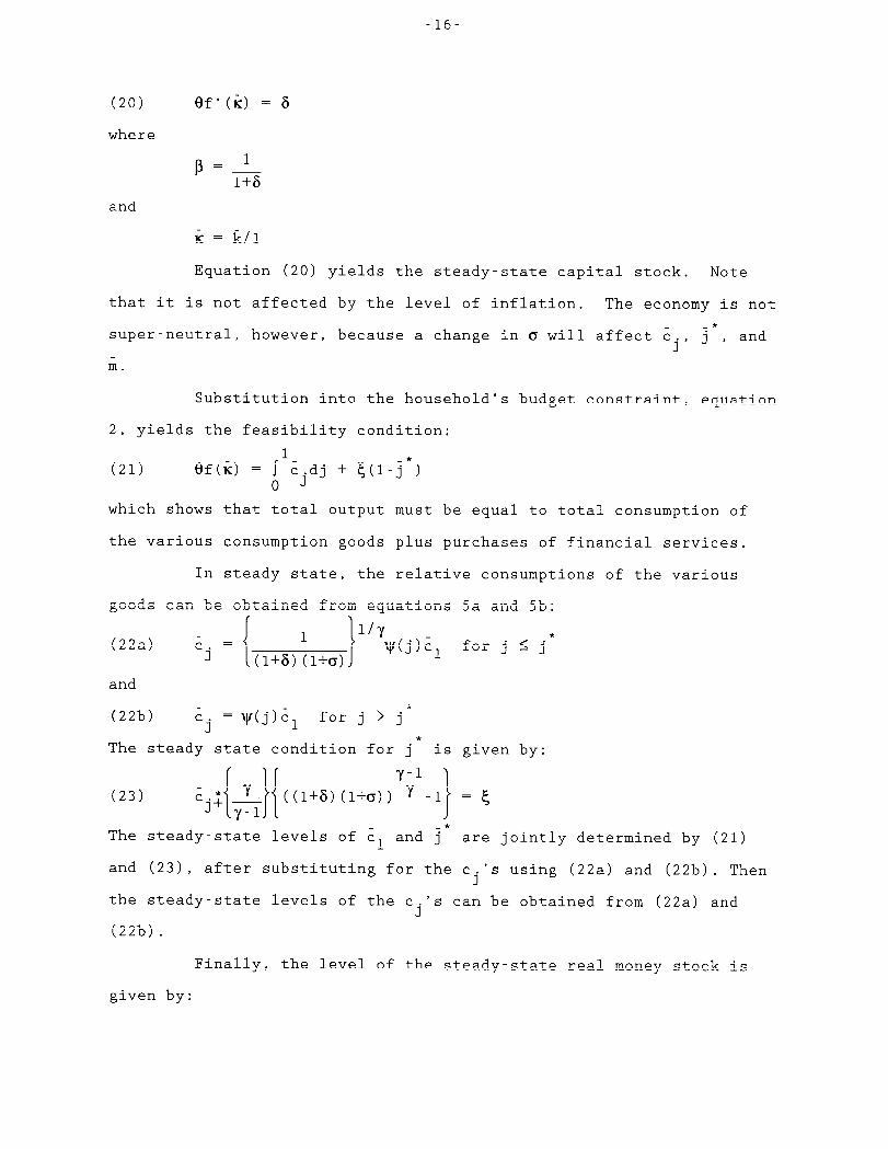
Finally, the level of the steady-state real money stock is

given by:

-17”

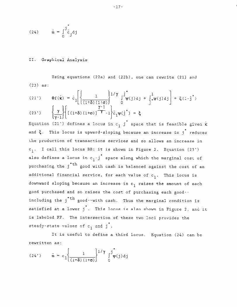
(24)

II. Graphical Analysis

Using

(23) as:

(21‘) ef(K)

(23‘){}Yy-1

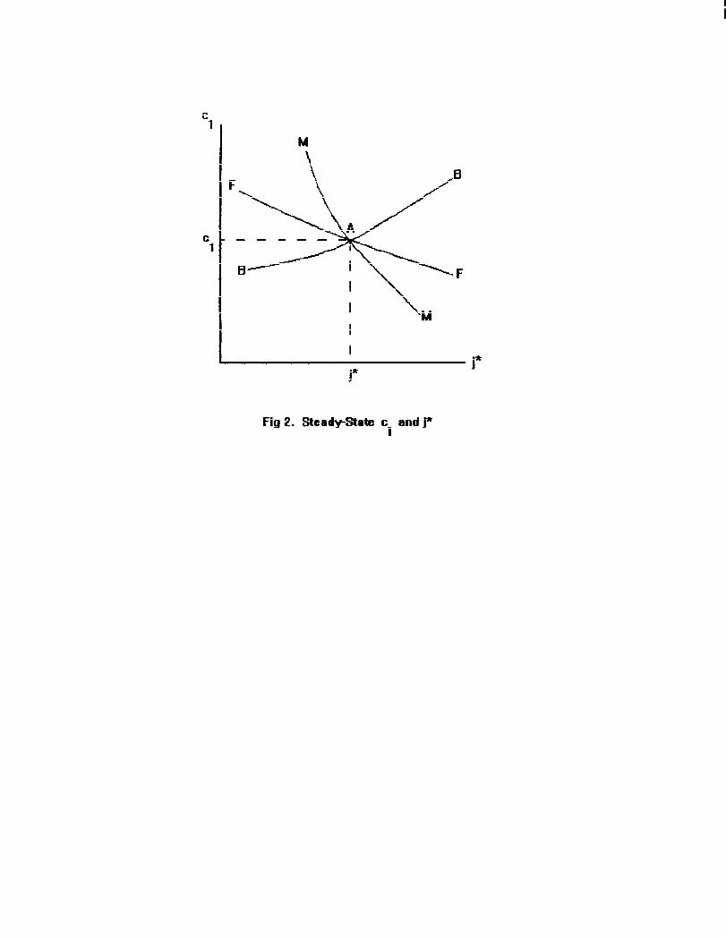
Equation (21’)

equations (22a) and (22b), one can rewrite (21) and

defines a locus in c1-j* space that is feasible given K

and ~. This locus is upward-sloping because an increase in j* reduces

the production of transactionsservices and so allows an increase in

c1“ I call this locus BB; it is shown in Figure 2. Equation (23‘)

also defines a locus in c1-j* space along which the marginal cost of

*thpurchasing the j good with cash is balanced against the cost of an

additional financial service, for each value of c1“

This locus is

downward sloping because an increase in c1 raises the amount of each

good purchased and so raises the cost of purchasing each good--

including the j‘th good--withcash. Thus the marginal condition is*

satisfied at a lower j . This locus is also shown in Figure 2, and it

is labeled FF. The intersectionof these two loci provides the*

steady-statevalues of c~ and j .

It is useful to define a third locus. Equation (24) can be

rewritten as:

‘24’)‘n=c,{(l+b,;l+a)l’’y r~(j)dj

-18-

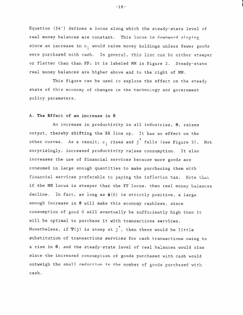
Equation (24’) defines a locus along which the steady-statelevel of

real money balances are constant. This locus is downward sloping

since an increase in c~ would raise money holdings unless fewer goods

were purchased with cash. In general, this line can be either steeper

or flatter than than FF; it is labeled MM in Figure 2. Steady-state

real money balances are higher above and to the right of MM.

This figure can be used to explore the effect on the steady

state of this economy of changes in the technology and government

policy parameters.

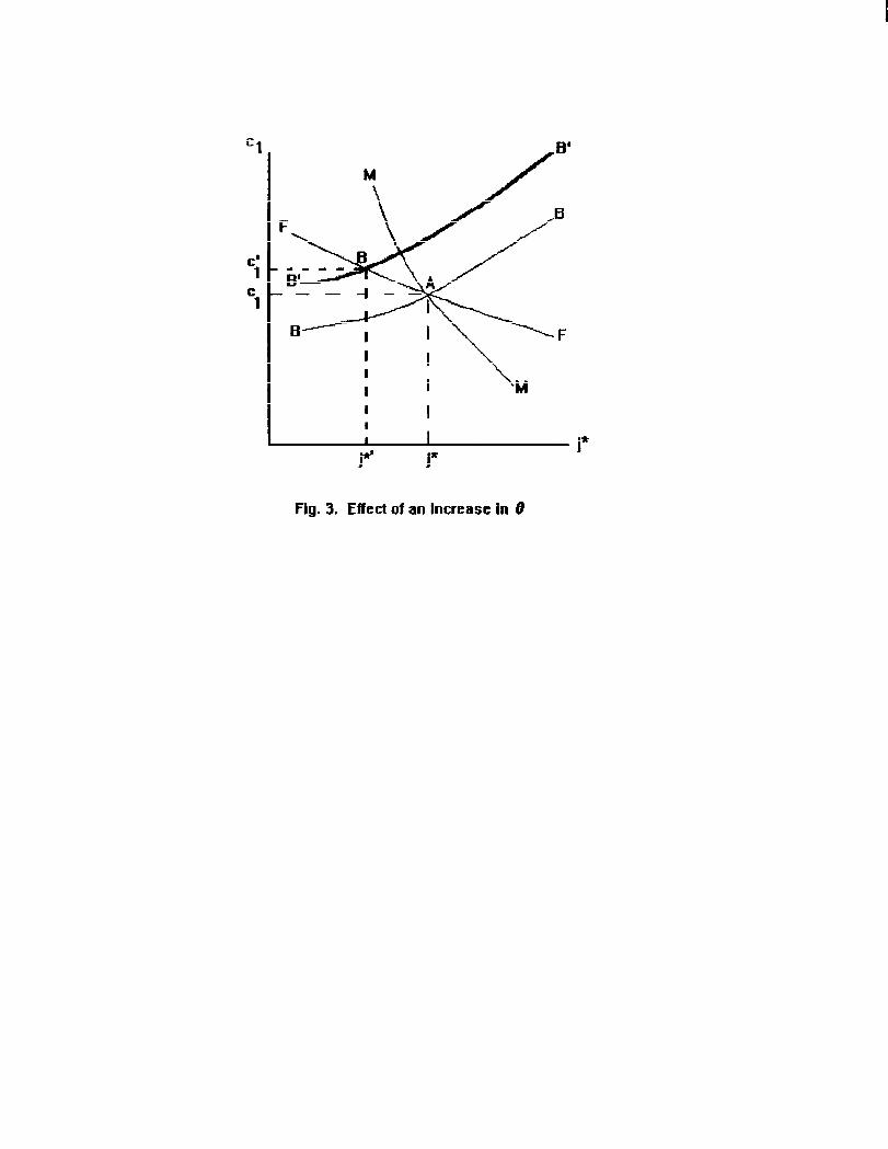
A. The Effect of an increase in 0

An increase in productivityin all industries,e, raises

output, thereby shifting the BB line up. It has no effect on the

other curves. As a result, c1 rises and j* falls (see Figure 3). Not

surprisingly,increased productivityraises consumption. It also

increases the use of financial services because more goods are

consumed in large enough quantitiesto make purchasing them with

financial services preferable to paying the inflation tax. Note that

if the MM locus is steeper than the FF locus, then real money balances

decline. In fact, as long as O(O) is strictly positive, a large

enough increase in e will make this economy cashless, since

consumptionof good O will eventuallybe sufficientlyhigh than it

will be optimal to purchase it with transactionsservices.*

Nonetheless, if~(j) is steep at j , then there would be little

substitutionof transactionsservices for cash transactionsowing to

a rise in e, and the steady-statelevel of real balances would rise

since the increased consumptionof goods purchasedwith cash would

outweigh the small reduction in the number of goods purchasedwith

cash.

-19-

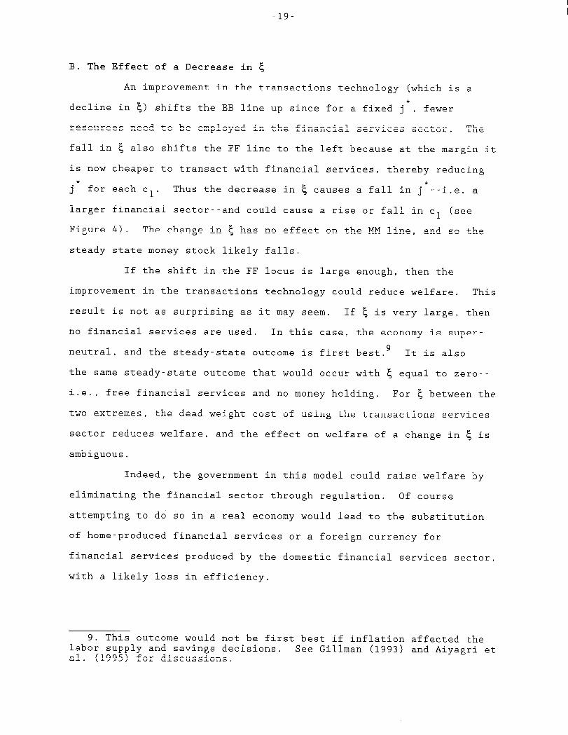
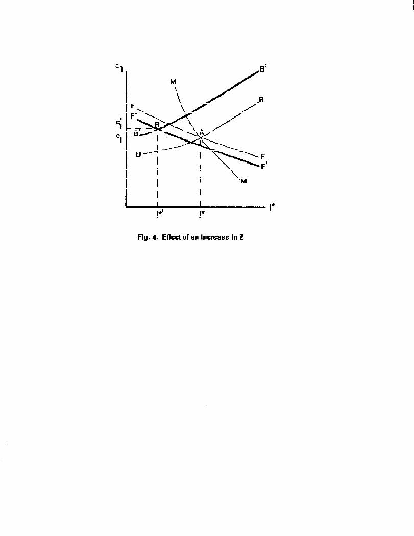
B. The Effect of a Decrease in ~

An improvementin the transactionstechnology (which is a

decline in ~) shifts the BB line up since for a fixed j*, fewer

resources need to be employed in the financial services sector. The

fall in { also shifts the FF line to the left because at the margin it

is now cheaper to transact with financial services, thereby reducing

j* for each cl. Thus the decrease in ~ causes a fall in j*--i.e. a

larger financial sector--andcould cause a rise or fall in c1 (see

Figure 4). The change in & has no effect on the MM line, and so the

steady state money stock likely falls.

If the shift in the FF locus is large enough, then the

improvementin the transactionstechnology could reduce welfare. This

result is not as surprisingas it may seem. If ~ is very large, then

no financial services are used. In this case, the economy is super-

9neutral, and the steady-stateoutcome is first best. It is also

the same steady-stateoutcome that would occur with { equal to zero--

i.e., free financial services and no money holding. For ~ between the

two extremes, the dead-weightcost of using the transactions services

sector reduces welfare, and the effect on welfare of a change in & is

ambiguous.

Indeed, the governmentin this model could raise welfare by

eliminatingthe financial sector through regulation. Of course

attempting to do so in a real economy would lead to the substitution

of home-producedfinancial services or a foreign currency for

financial services produced by the domestic financial services sector,

with a likely loss in efficiency.

9. This outcome would not be first best if inflation affected thelabor supply and savings decisions. See Gillman (1993) and Aiyagri etal. (1995) for discussions.

-20-

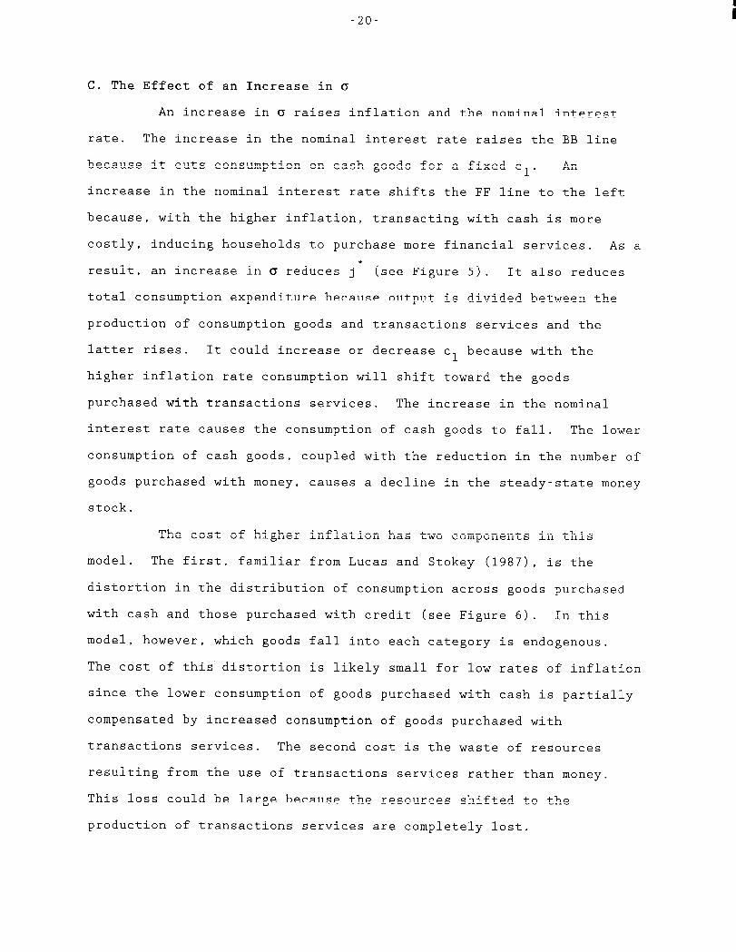
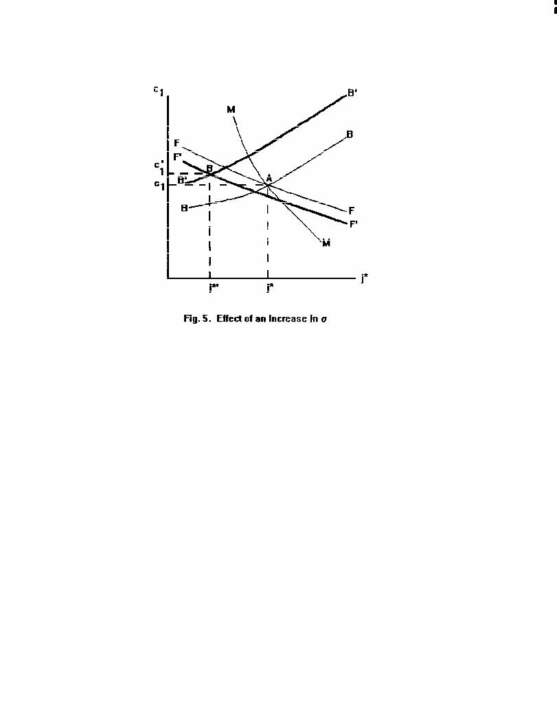
C. The Effect of an Increase in c

i

An increase in a raises inflation and the nominal interest

rate. The increase in the nominal interest rate raises the BB line

because it cuts consumptionon cash goods for a fixed cl. An

increase in the nominal interest rate shifts the FF line to the left

because, with the higher inflation,transactingwith cash is more

costly, inducing households to purchase more financial services. As a

result, an increase in 6 reduces j* (see Figure 5). It also reduces

total consumptionexpenditurebecause output is divided between the

production of consumption goods and transactionsservices and the

latter rises. It could increase or decrease c1 because with the

higher inflation rate consumptionwill shift toward the goods

purchased with transactions services. The increase in the nominal

interest rate causes the consumptionof cash goods to fall. The lower

consumptionof cash goods, coupled with the reduction in the number of

goods purchasedwith money, causes a decline in the steady-statemoney

stock.

The cost of higher inflation has two components in this

model. The first, familiar from Lucas and Stokey (1987),is the

distortion in the distributionof consumptionacross goods purchased

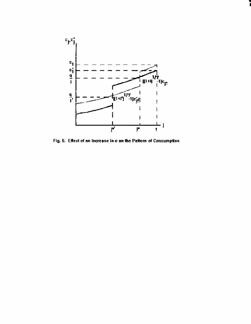
with cash and those purchased with credit (see Figure 6). In this

model, however, which goods fall into each category is endogenous.

The cost of this distortion is likely small for low rates of inflation

since the lower consumptionof goods purchasedwith cash is partially

compensatedby increased consumptionof goods purchased with

transactions services. The second cost is the waste of resources

resulting from the use of transactionsservices rather than money.

This loss could be large because the resources shifted to the

production of transactionsservices are completely lost.

-21-

The optimal monetary policy in this economy is clearly to set

~ sufficientlylow that all purchases are made with cash. If ~(j) is

bounded, as assumed above, this policy will not correspond to a zero

nominal interest rate, as in the Friedman rule. So long as the

nominal interest rate is low enough that it is cheaper to buy good 1

with cash than with purchased transactionsservices, there will be no

cost to the inflation. If one allowed ~(j) to go to infinity as j

goes to 1, then the usual Friedman rule would obtain.10

III. Empirical Evidence

In the Introduction,I noted the evidence from the 1920s on

the effect of hyperinflationon the size of the financial sector. A

similar effect has been noted in the cases of Brazil and Israel in the

1980s. Dornbusch et al. (1990,p. 25) note that in Brazil “financial

markets substantiallyadapted [to high inflation]. As a result, the

velocity of Ml rose more than in other countries,while that of M4

increased less. The sharp rise in the velocity of Ml reflects a well

organized payment system by check (even for a lunch snack) drawn on

overnight accounts.~ Presumably this “well-organized”payment system

required increased capital and labor in the financial sector.

Marom (1988),presents an empirical study of the effects of

inflation on the size of the banking sector in Israel in the early

1980s. He notes that while the share of banking in Israeli GDP in

1970 was smaller than in any of the six OECD countries for which

10. The Friedman rule would also obtain, regardless of theboundedness of ~, if inflation affected the labor or savingsdecisions. Aiyagari et al. (1995) and Cooley and Hansen (1991) arguethat these distortionscould be important.

-22-

comparable data are available, it was larger than in all of the six

OECD countries by 1982. Over the period 1970-82 inflation in Israel

averaged 33.9 percent, more than three times the highest average rate

among the OECD countries. Marom estimates a time series econometric

model to assess the effect of inflation on the size of the Israeli

banking sector. The effects are statisticallysignificantand

indicate that high inflation (definedby Marom as inflation over 10

percent per year) nearly doubled the share of banking in GDP in the

early 1980s. Similar equations estimated using banking’s share in

total employment and total wages show smaller but statistically

significanteffects.

Work by Kleiman (1989) provides informationon the effect of

the 1984 stabilizationprogram on employment in the banking sector.

After expanding further in 1983, employment declined through 1987, by

which time it had returned to its 1979 level. As noted by Kleiman,

however, the immediate cause of the decline was a banking crisis that

occurred in late 1983. The governmentintervened to provide

assistance,but the banks were required to cut costs. Nonetheless,

the pattern of banking sector expansion and contractionis broadly

consistentwith the model.

Aiyagari et al. (1995) present time series data on the size

of the banking sector in Brazil, Israel, and Argentina, noting that

high inflation has been reflected in the size of the financial sector

in all three countries. The Argentine data, however, is somewhat

problematical: The banking sector’s share in employment peaked around

1980 and then declined,while the inflation rate spiked sharply in the

mid-1980s, and then even more forcefully later in the decade. The

decline in the relative size of the financial sector in the early

1980s likely reflected the effects of a financial crisis at that time,

-23-

which followed a period of financial liberalizationin the late 1970s

(Balino,1991). As a result, when inflation picked up in the mid- and

late-1980sArgentineans appear to have reacted, at least in part, by

shifting to U.S. dollars rather than making greater use of domestic

financial firms (Dornbuschet al., 1990, p. 25).11 Currency

substitutionof this sort is, of course, another form of costly

adjustment to high inflation--albeit one of a sort not contemplatedin

the model.

A. A Cross-CountryComparison

As an alternativetest of the model, similar to Marom’s

(1988) comparison of Israel to six OECD countries, I consider a

cross-countrycomparison of inflation rates and financial sector

size. The model presented above suggests that the share of output

devoted to the financial sector should be a function of the level of

inflation, output per capita, and relative productivityin the

financial sector. While higher inflation should cause the financial

sector to expand, the effects of the other two variables are not clear

on theoretical grounds. As noted in section II, above, higher

productivitywill raise consumptionof all goods, causing an increase

in the number of transactionsthat are made without cash. It is not

clear, however, whether the proportionalincrease in the financial

sector will be larger or smaller than that of GDP. Similarly,more

transactionswill be done with financial services if the financial

11. The resulting difference in the method of domestic payments isnoted in a recent Economist survey of Latin American Finance (Dec. 9-15, 1995). Kamin and Ericsson (1993) present an empirical study ofdollarizationin Argentina. They conclude that holdings of U.S.dollar currency in Argentina were nearly as large as the total ofdollar-denominateddomestic deposits and all peso-denominatedmonetaryassets by the early 1990s. They also note that the effect ofinflation on the use of dollars appears to be long lived.

-24-

sector becomes more efficient,but the relative price of these

services will fall. Thus, the net effect of the productivityincrease

on the financial sector’s share is uncertain.

Because of the difficulty of obtaining comparable information

on the relative size of the banking sector for a large number of

countries, I focus on the broader sector including finance, insurance,

and real estate. I use two measures of the size of the financial

sector: its share in GDP and its share in employment (both in

percent). These shares can be used to calculate the relative

productivityof labor in the financial sector. Because data on

capital inputs are not available, a more comprehensivemeasure of

total factor productivitycannot be constructed. The GDP, employment,

and labor productivitydata are for 1985.12 Wherever possible, I

measure annual average percentage inflation using the GDP deflator.

Where this is not available, the consumer price index has been

substituted. Because the model presented above focused on steady

states, I use the average annual inflation rate over the ten years

from 1975 to 1985.13 To account for differencesin the level of

income across countries, I use GNP per capita at world prices from the

Penn World Table (Summersand Heston, 1991). For details on the data

used, see the data appendix.

B. Empirical Results

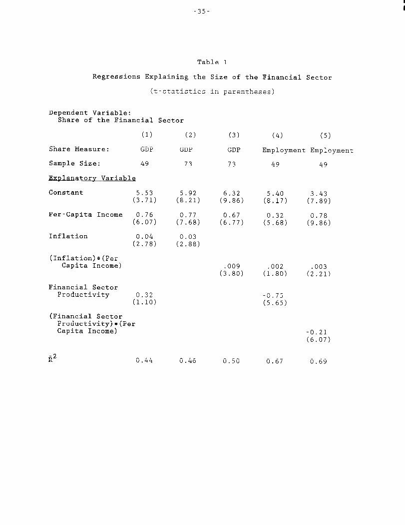
The first column of table 1 shows the results of a regression

of the share of the financial sector in GDP on per-capita real output,

average inflation over the previous 10 years, and relative labor

12. In some cases the employment data were not available for 1985,and so data from 1984, 1986, or 1987 were substituted.13. I experimentedwith the average inflation rate over 1980-85 and

obtained similar results.

-25-

productivityin the financial sector. The results show that higher

levels of per-capita income and average inflation are reflected in

increased financial sector size. By contrast, there does not appear

to be a significanteffect of relative labor productivityon this

measure of financial sector size. This result suggests that the two

offsetting effects noted above cancel out. Dropping the productivity

variable from the regression,as shown in the second column, does not

greatly affect the other parameters.

The strong and statisticallysignificanteffect of real

income per capita on the size of the financial sector should not come

as a surprise. Kuznets (1971, p. 107) notes that ‘the share of

banking, insurance and real estate shows a striking rise as we shift

from low to higher income countries.” The strong result found here

suggests that either the effect of higher income on the share of goods

purchased without cash is large, or the model fails to capture another

effect of higher income that leads to increased use of the financial

system. It is not hard to think of such effects. For example, if

higher income households purchase a larger number of goods, as well as

more of each good, higher incomes would lead to a larger number of

transactionsand likely to an increased need for financial services

(as well as cash). Alternatively,if households do their own cash

management, they may choose to do less of it as incomes rise, owing to

the higher opportunity cost of household time. As a result,

households would increase their purchases of transactionsservices

produced by financial firms.

The effect of inflation on the size of the financial sector,

as shown in columns 1 and 2, is economicallyas well as statistically

significant. Given that countrieswith higher per-capita incomes

generallyhave larger financial sectors, however, it seems likely that

-26- i

the effect of inflation on financial sector size is larger in high

income countries as well. To test this hypothesis I interact the

inflation term with per capita income in the regression reported in

14column 3. The use of the interactionterm improves the fit of the

regressionfairly substantially,suggestingthat the effect of

inflation on the size of the financial sector is smaller for low-

income than for high-income countries.

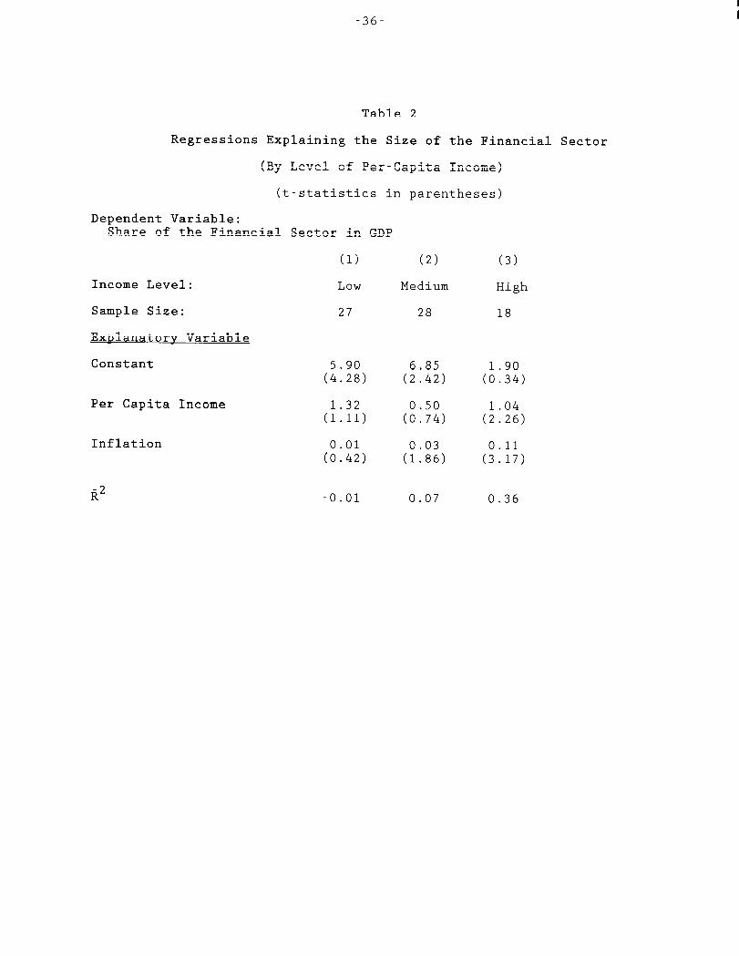
The results of an alternativetest are shown in table 2.

Here the countries are divided into three groups based on income per

capita, and for each group a separate regressionis run of financial

15sector size on income and average inflation. The coefficienton

the inflation rate is small and insignificantfor the poorest

countries,moderate and marginally significantfor the middle-income

countries, and large and significantfor the high-income countries.

The theoreticalmodel suggests that the effect of inflation

on financial sector size should be nonlinear. In particular,if

inflation gets sufficientlyhigh, virtually all transactionsare done

without money. Further increases in inflationwill then have no

effect on the size of the financial sector. Experimentationwith a

number of nonlinear specifications,however, did not yield

statisticallysignificantnonlinearities.

The remaining columns in table 1 show regression results for

the share of the financial sector in total employment. One difference

between the GDP share and employment share results is the significance

of the productivityvariable in the employment regressions,especially

14. If the level of inflation is included as well as the interactionterm, it is insignificantand does not affect the other parameters.15. The income categorieswere defined, arbitrarily,as under $2000,

between $2000 and $9000, and over $9000. The mean income level in thesample is about $4800. Modest changes in the cutoff levels of incomedo not affect the results appreciably so long as Israel (with a 1985per capita income of $9293) remains in the high income group.

-27-

when it is interactedwith the level of income (column5). Given the

insignificanceof this variable in the GDP regression,the

significancehere may not be a surprise. Since countrieswith higher

financial sector labor productivitydo not generallyhave a larger

share of GDP in the financial sector, they must have a smaller share

of employment in the sector. The inflation interactionterm is

significantin the employment regressions,although the coefficientis

less than 1/3 the size of the comparable term in the GDP regressions.

The smaller parameter is not surprisingbecause, on average, the share

of the financial sector in employment is about 1/3 as large as its

share in GDP, suggestinga similar proportionaldecline in the size of

the parameter.

C. Caveats

There are two caveats to the empirical results shown above.

First, it is possible that the relatively large effect of inflation on

the GDP measure of financial sector size reflects inflation-induced

measurement error. The measurement of output in the financial sector

is difficult because output is often hard to quantify. (See Triplett,

1993, for a brief discussion of the difficultiesin measuring banking

sector output.) If, for example, high inflation led to an upward bias

in the measurement of financial sector output, then the regression

results would reflect, in part, the measurement problem rather than a

real effect of inflation.

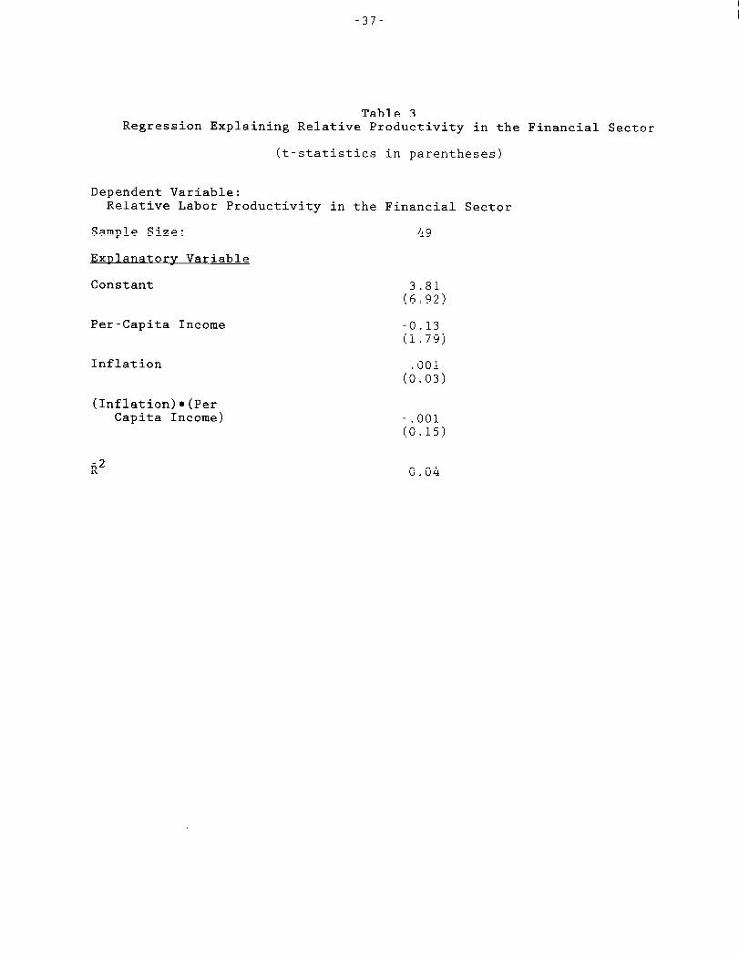
Such a bias should be apparent in the labor productivity

measure used in the regressions,since the share of the financial

sector in GDP would be boosted by the measurement error while the

-28-

16share of the financial sector in employmentwould not be. To test

for this effect, I regress the productivitymeasure on per capita

income, inflation, and inflation times per capita income. The

results, shown in table 4, show no significanteffect of either

inflation variable on relative labor productivityin the financial

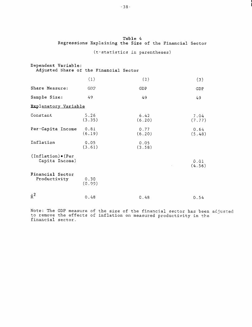
sector. Table 5 shows the results of regressionslike those in table

1 when the GDP measure of financial sector size is adjusted to remove

the effects of inflation on relative financial sector productivity

shown in table 4. These adjusted results differ very little from the

baseline results in table 1.17

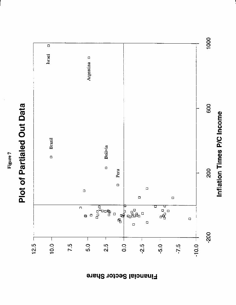
A second caveat is simply to point out the importance in the

empirical results of a relatively small number of countries. Figure 7

shows a plot of the GDP measure of financial sector size versus

inflation times per capita income. (A constant and per capita income

have been partialed out of both variables.) The upward slope found in

the regressionsis clearly evident in the figure. It is also clear,

however, that the result depends a great deal on a small number of

countrieswith very high inflation rates. The five most inflationary

countries in the sample--Israel,Argentina, Brazil, Bolivia, and

Peru--comprise5 of the 6 observationsin the upper-right quadrant of

16. The relative labor productivitymeasure is:(FinancialSector GDP)/(FinancialSector Emt)lovment)

(TotalGDP)/(TotalEmployment)which can be rewritten as:

(FinancialSector GDP)/(TotalGDP)(FinancialSector Employment)/(Total Employment)

which is the ratio of the financial sector share in GDP to thefinancial sector share in employment.17. To do the adjustment, I started by adjusting the relative

productivityvariable by evaluating the two inflation terms in theregressionand subtractingthem from the relative productivitymeasure. Then I multiplied this adjusted productivitymeasure by theshare of the financial sector in employmentto get the adjustedmeasure of the financial sector in GDP.

-29-

the figure.18 If they are excluded from the regressions,the

inflation terms are no longer significant. However, excluding them is

surely wrong, since high inflation countries are exactly the ones with

the most informationabout the effects of inflation on financial

sector size.

Nonetheless. it is unfortunatethat the effect of inflation

on financial sector size does not stand out in the lower inflation

countries. Evidently, other factors contribute importantlyto

variation in the size of countries’ financial sectors. In part, this

variation likely reflects the effects of regulationand past financial

sector difficulties. In addition, the regressionsemploy data on the

production of financial services,while it is consumptionof financial

services that should be affected by inflation. Clearly, if a country

purchases financial services from firms in a neighboring country, its

financial sector will appear to be unexpectedlysmall, while that of

its neighbor will appear to be large. The geographicalpattern of the

residuals suggests that this differencemay be significantin some

cases. For example, the residual for Belgium in the regression shown

in column 3 of table 1 is -8.3 percent, the financial sector in

Luxembourg is more than 9 percent larger than the equation would lead

you to expect (becauseof its small population,Luxembourgwas

excluded from the regression). By contrast, the standard error of the

regression is only 3.6 percent. Similarly,the residual for Ireland

is -5.8 percent, while that for the United Kingdom is +3.6. In some

cases there appear to be regional financial centers reflecting

relative political or economic stability. In particular,Jordan and

Kenya have unexpectedlylarge financial sectors (residualsof 6.2 and

18. The other one is Chile, which had the seventh highest inflationrate in the sample.

-30-

6.0 percent respectively), while some of their neighbors have

unexpectedly small ones. Note that to the extent that low inflation

allows a country to export financial services to its neighbors, low

rather than high inflationwould be associatedwith a large financial

sector, biasing downward the estimated effect of inflation on the size

of the financial sector.

D. Discussion

The regressions shown in table 1 suggest a larger cost of

inflation than might have been expected. A 10 percent rise in the

inflation rate in the U.S. (1985 real per-capita income, $16,779)

would be expected to increase the share of the financial sector in GDP

by about 1-1/2 percent, and its share in employmentby about 1/2

percent. The 1-1/2 percent share of GDP is a measure of the resources

lost owing to the inflation. Fischer (1981) and Lucas (1981)

calculate that the welfare loss of a 10 percent inflation amounts to

.3 to .45 percent of GNP, based on estimates of the area under a money

demand curve. However, Lucas (1994) reports a welfare loss similar

to that reported here, 1.3 percent, based on a different

paramaterizationof the money demand curve. It is straightforwardto

show that, in the model presented above, the area under the

compensatedmoney demand curve is approximatelyequal to the size of

the financial sector.19 Thus the results presented here do not

differ conceptuallyfrom the measures employed by Fischer and Lucas.

To assess whether the large costs of inflation found here are

credible, table 5 presents informationon the two measures of

financial sector size, inflation, and per-capita income for the five

19. The two are exactly equal if inflation is not allowed to distortthe pattern of consumptionacross goods. For a proof of a similarresult, see Aiyagari et al. (1995).

-31-

countrieswith the highest inflation rates over 1975-85. Also

reported in the table are the average values of these variables for

other countries with real per-capita incomes between 50 and 150

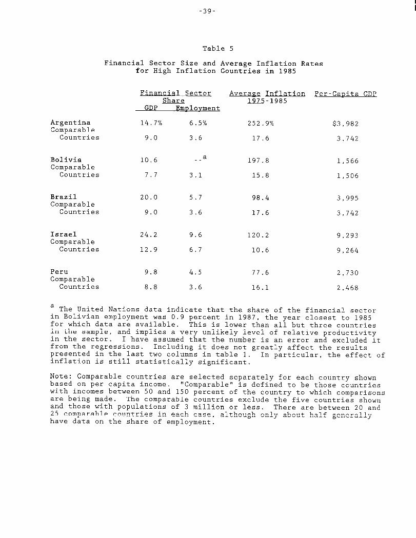
percent of each of the five countries. As shown in the table, both

Brazil and Israel have financial sector shares in GDP more than 10

percentage points larger than other comparable countries. By the same

measure, Argentina, Bolivia, and Peru have financial sectors that

roughly 6, 3, and 1 percentage point larger than their peers. With

the exception of Bolivia, there is a similar pattern to the employment

shares of the financial sector, with financial sector employment 3

percentage points higher in Argentina, Brazil, and Israel, and 1

percentage point higher in Peru.

It is not surprisingthat the effects of inflation on

financial sector size are largest for Brazil and Israel, and smaller

in the other three countries. As noted above, a larger share of the

adjustment to inflation in Argentina took the form of dollarization.

The same appears to have been the case in Bolivia (Melvin,1988;

Melvin and Afcha, 1989) and Peru (Rojas-Suarez,1992). The experience

in these countries suggests that high inflationmay not lead to as

large an expansion in the financial sector if currency substitution

takes place instead. Which method of adjustment predominates

presumably depends on the regulatory environmentas well as the

quality of financial firms at the start of the inflation. In any

case, the likely importance of dollarizationin limiting the size of

the financial sector in some of the high inflation countries suggests

that the regression results reported above will provide underestimates

of the effects of inflation on financial sector size for countries

where growth in the financial sector is not constrainedby regulation

or financial crises.

-32-

The evident large effects of inflation shown in table 3 are

consistentwith the large costs of modest inflations implied by the

regressions. For example, Israel, with 110 percentage points of

“extra” inflation relative to its peers, had a financial sector share

about 11 percentage points higher, implying a cost of about 1 percent

of GDP for each 10 percent of inflation. For the U.S., with per

capita income about half again as large, an increase of 1-1/2 percent

for a 10 percent inflation seems plausible.

Aiyagari et al. (1995) report that the effects of inflation

on the banking sector appear to be limited to a few percent of GDP.

Thus the larger effects found here for the broader finance, insurance,

and real estate sector likely reflect, in part, increases in other

subsectorsas well as in banking. This implication seems plausible:

other intermediaries, such as insurance companies and securities

dealers will have to handle more transactionsas businesses and

households increase their efforts to conserve on cash. Moreover, such

firms will also be boosting their own efforts to limit cash holdings.

Of course institutionalinertia or nonlinearitiescould limit

the expansion of the financial sector in response to moderate

inflations, reducing the cost of such inflationsto levels below those

implied by the estimated equations. There are other reasons, however,

to believe that the increase in the size of the financial sector

understatesthe total costs of inflation. For example, this measure

does not take account of the unremuneratedcosts of increased “home

production”of financial services--e.g.the traditional shoeleather

costs of inflation--nor does it account for the production of

financial services by nonfinancialfirms. Bresciani-Turroni(1937)

notes that during the German hyperinflationnonfinancialfirms had to

-33-

greatly increase the amount of “unproductive”work time--i.e., work

required to manage financial flows.

The increase in the size of the financial sector also does

not take account of a variety of other inflation-relateddistortions.

For example, the wedge driven between the marginal utility of cash and

non-cash goods in consumption reduces welfare directly. Similar

distortions in labor supply and investment decisions reduce welfare

indirectlyby reducing either current or future output. Even if

consumptionand investmentwould otherwise not be affected, if

reserves pay no interest, inflation serves as a tax on intermediation,

reducing the efficiency of resource allocation. Finally, there is

some evidence (see Fischer, 1993) that inflation reduces the growth

rate of total factor productivity,which would have a potentially

large effect on welfare.

-34-

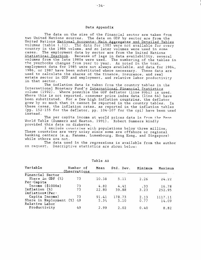
Data Appendix

The data on the size of the financial sector are taken fromtwo United Nations sources. The data on GDP by sector are from theUnited Nations National Accounts: Main A~~re~ates and Detailed Tablesvolumes (table 1.11). The data for 1985 were not available for everycountry in the 1986 volume, and so later volumes were used in somecases. The employment data by sector are from the United NationsStatisticalYearbook. Because of lags in data availability,severalvolumes from the late 1980s were used. The numbering of the tables inthe yearbooks changes from year to year. As noted in the text,employment data for 1985 were not always available, and data for 1984,1986, or 1987 have been substitutedwhere necessary. These data areused to calculate the shares of the finance, insurance, and realestate sector in GDP and employment,and relative labor productivityin that sector.

The inflation data is taken from the country tables in theInternationalMonetary Fund’s InternationalFinancial Statisticsvolume (1992). Where possible the GDP deflator (line 99bi) is used,Where this is not reported, consumer price index data (line 64) havebeen substituted. For a few high inflation countries,the deflatorgrew by so much that it cannot be reported in the country tables. Inthese cases, the inflation rates, as reported in the inflation tables(pp. 152-155 for the deflator, pp. 104-107 for the cpi) have been usedinstead.

The per capita income at world prices data is from the PennWorld Table (Summersand Heston, 1991). Robert Summers kindlyprovided this data on diskette.

I exclude countrieswith populationsbelow three million.These countries are very noisy since some are offshore or regionalbanking centers (e.g. Panama, Luxembourg,Hong Kong, and Singapore)while others are not.

The data used in the regressionsis available from the authoron request. Descriptive statisticsare shown below:

Table Al

Variable Number of Mean Std. Dev. Minimum MaximumObservations

Financial SectorShare in GDP (%) 73 10.38 5.11 2.26 24.22

Per-CapitaIncome ($1000s) 73 4.82 4.41 .33 16.78

Inflation (%) 73 22.80 39.88 3.23 252.95Inflationo(Per-Capita Income) 73 91.41 178.73 2.13 1117.11

Share in Employment (%) 49 5.34 3.10 0.77 14.09Relative LaborProductivity 49 2.99 2.02 0.40 8.82

-35-

Table 1

RegressionsExplaining the Size of the Financial Sector

(t-statisticsin parentheses)

Dependent Variable:Share of the Financial Sector

(1) (2) (3)

Share Measure: GDP GDP GDP

Sample Size: 49 73 73

ExplanatoryVariable

Constant 5.53 5.92 6.32(3.71) (8.21) (9.86)

Per-Capita Income 0.76 0.77 0.67(6.07) (7.68) (6.77)

Inflation 0.04 0.03(2.78) (2.88)

(Inflation)o(PerCapita Income)

Financial SectorProductivity 0.32

(1.10)

(FinancialSectorProductivity)o(perCapita Income)

(4) (5)

Employment Employment

49 49

5.40 3.43(8.17) (7.89)

0.32 0.78(5.68) (9.86)

009 .002(~.80) (1.80)

-0.75(5.65)

.003(2.21)

-0.21(6.07)

R2 0.44 0.46 0.50 0.67 0.69

-36-

Table 2

Regressions Explaining the Size of the Financial Sector

(By Level of Per-Capita Income)

(t-statisticsin parentheses)

Dependent Variable:Share of the Financial Sector in GDP

(1) (2) (3)

Income Level:

Sample Size:

ExplanatoryVariable

Constant

Per Capita Income

Inflation

Low Medium High

27 28 18

5.90 6.85 1.90(4.28) (2.42) (0.34)

1.32 0.50 1.04(1.11) (0.74) (2.26)

0.01 0.03 0.11(0.42) (1.86) (3.17)

R2 -0.01 0.07 0.36

-37-

Table 3Regression Explaining Relative Productivityin the Financial Sector

(t-statisticsin parentheses)

Dependent Variable:Relative Labor Productivity in the Financial Sector

Sample Size: 49

ExplanatoryVariable

Constant 3.81(6.92)

Per-Capita Income

Inflation

(Inflation)o(PerCapita Income)

-0.13(1.79)

.001(0.03)

-.001(0.15)

R2 0.04

-38-

Table 4RegressionsExplaining the Size of the Financial Sector

(t-statisticsin parentheses)

Dependent Variable:Adjusted Share of the Financial Sector

(1) (2)

Share Measure: GDP GDP

Sample Size: 49 49

ExDlanatorvVariable

(3)

GDP

49

Constant

Per-Capita Income

Inflation

(Inflation)o(PerCapita Income)

Financial SectorProductivity

R2

5.26 6.42(3.35) (6.20)

0.81 0.77(6.19) (6.20)

0.05 0.05(3.61) (3.58)

7.04(7.77)

0.64(5.48)

0.01(4.56)

0.30(0.99)

0.48 0.48 0.54

Note: The GDP measure of the size of the financial sector has been adjustedto remove the effects of inflation on measured productivityin thefinancial sector.

-39-

ArgentinaComparableCountries

BoliviaComparableCountries

BrazilComparableCountries

IsraelComparableCountries

PeruComparableCountries

a The United

Table 5

Financial Sector Size and Average InflationRatesfor High Inflation Count~ies in 1985

Financial SectorShare

GDP EmRlovment

14.7% 6.5%

9.0 3.6

10.6 a.-

7.7 3.1

20.0 5.7

9.0 3.6

24.2 9.6

12.9 6.7

9.8 4.5

8.8 3.6

Nations data indicate that

Average Inflation1975-1985

252.9%

17.6

197.8

15.8

98.4

17.6

120.2

10.6

77.6

16.1

Per-CaDitaGDP

$3,982

3,742

1,566

1,506

3,995

3,742

9,293

9,264

2,730

2,468

the share of the financial sectorin Bolivian employmentwas 0.9 percent in 1987, the year closest to 1985for which data are available. This is lower than all but three countriesin the sample, and implies a very unlikely level of relative productivityin the sector. I have assumed that the number is an error and excluded itfrom the regressions. Including it does not greatly affect the resultspresented in the last two columns in table 1. In particular,the effect ofinflation is still statisticallysignificant.

Note: Comparable countries are selected separatelyfor each country shownbased on per capita income. “Comparablenis defined to be those countrieswith incomes between 50 and 150 percent of the country to which comparisonsare being made. The comparable countries exclude the five countries shownand those with populationsof 3 million or less. There are between 20 and25 comparable countries in each case, although only about half generallyhave data on the share of employment.

-40-

REFERENCES

Aiyagari, S. Rae, and Zvi Eckstein, “Interpreting MonetaryStabilizationin a Growth Model with Credit Goods Production,HFederal Reserve Bank of Minneapolis Working Paper No. 525, 1994.

, and Toni Braun, “TransactionsServices,Inflation:and Welfare,n Federal Reserve Bank of MinneapolisWorkingPaper No. 551, July 1995.

Balino, Thomas J. T., “The Argentine Banking Crisis of 1980,” inSundararajanV., and Thomas J. T. Balino, Banking Crises: Cases andIssues, Washington,D.C.: InternationalMonetary Fund, 1991.

Baumol, William J., “The TransactionsDemand for Cash: An inventorytheoretic approach,” Quarterly Journal of Economics, 1952, pp. 545-556.

Bresciani-Turroni, Costantino,The Economics of Inflation:A Studv ofCurrencv Depreciation in Post-War Germanv, translatedby Millicent E.Sayers, London: George Allen and Unwin, Ltd., 1937.

Cole, Harold L. and Alan C. Stockman, “Specialization,TransactionsTechnologies,and Money Growth,U InternationalEconomic Review, 1992,PP” 283-298.

Cooley, Thomas and Gary Hansen, ‘The Welfare Costs of ModerateInflations,”Journal of Money, Credit. and Banking, 1991, pp. 483-503.

Dornbusch, Rudiger, Federico Sturzenegger,and Holger Wolf, “ExtremeInflation:Dynamics and Stabilization,nBrookin~s PaDers on EconomicActivitv 2, 1990, pp. 1-64.

Dotsey, Michael and Peter Ireland, “On the Costs of Inflation inGeneral Equilibrium,”Mimeo. Federal Reserve Bank of Richmond, 1993.

Federal Reserve System, Functional Cost and Profit Analvsis: NationalAvera~e ReDort. CommercialBanks 1994, 1995.

Fischer, Stanley, “The Role of MacroeconomicFactors in Growth,nJournal of Monetarv Economics, 32(3), December 1993, pp. 485-512.

“A Framework for Monetary and Banking Analysis,n EconomicJournal, 1683, pp. 1-16.

. “Towards an Understandingof the Costs of Inflation: 11,”Carne~ie-RochesterConference Series on Public Policy 15, 1981, pp.5-41.

Gillman, Max. “The Welfare Cost of Inflation in a Cash-in-AdvanceEconomy With Costly Credit,” Journal of Monetary Economics, 1993, pp.97-116.

Humphrey, David B., Lawrence B, pulley, and Jukka Vesala, ~Cash,Paper, and Electronic Payments: A Cross Country Analysis,~ Mimeoo,Florida State University, 1995.

-41-

Kamin, Steven B. and Neil R. Ericsson, “Dollarizationin Argentina,HInternationalFinance Discussion Paper No. 460, Federal Reserve Board,1993.

Kleiman, Ephraim, “The Costs of Inflation,nDepartment of EconomicsWorking Paper No. 211, Hebrew University, 1989.

Kuznets, Simon, Economic Growth of Nations: Total Out~ut andProduction Structure, Cambridge,MA: Harvard University Press, 1971.

Lucas, Robert E. “On the Welfare Cost of Inflation,” Mimeo.,University of Chicago, 1994.

. “Discussionof ‘Towardsan Understandingof the Costs ofInflation: II,U CarneRie-RochesterConference Series on public policv15, 1981, pp. 43-52.

and Nancey L. Stokey, “Optimal Fiscal and MonetaryPolicies in an Economy Without Capital,U Journal of MonetarvEconomics, 1983, pp. 55-93.

and “Money and Interest in a Cash-in-AdvanceEconomy,N Econometric, 1;87, pp. 491-513.

Marom, Arie. “Inflationand Israel’s Banking Industry,” Bank of IsraelEconomic Review, 1988, pp. 30-41.

Melvin, Michael. “The Dollarizationof Latin America as a Market-Enforced Monetary Reform: Evidence and Implications,nEconomicDevelopment and Cultural Change 36, 1988, pp. 543-558.

and G. Afcha. “Dollar Currency in Latin America: A BolivianApplication,w Economics Letters 31, 1989, pp. 393-397.

Prescott, Edward C. “A Multiple Means-of-PaymentModel,n in Barnett,William A. and Kenneth J. Singleton,eds., New ADDroaches to MonetaryEconomics, Cambridge: Cambridge University Press, 1987.

Rojas-Suarez,Liliana. “CurrencySubstitutionand Inflation in Peru,URevista de Analisis Economico 7, 1992, pp. 153-176.

Romer, David, “A Simple General EquilibriumVersion of the Baumol-Tobin Model,” Quarterly Journal of Economics, 1986, pp. 663-685.

Schreft, Stacey L. “TransactionsCost and the Use of Cash and Credit,UEconomic Theorv, 1992, pp. 283-296.

Stockman,Alan, “AnticipatedInflation and the Capital Stock in aCash-in-AdvanceEconomy,H Journal of Monetarv Economics, 1981, pp.387-393.

Summers, Robert and AlIan Heston, “The Penn World Table (Mark 5): AnExpanded Set of InternationalComparisons,n Quarterlv Journal ofEconomics, 106(2), May 1991, pp. 327-368.

Tobin, James, ‘The Interest Elasticity of the TransactionsDemand forCash,U Review of Economics and Statistics, 1956, pp. 241-47.

-42-

Triplett, Jack E. “Banking Output” in Newman, peter, Murray Milgat~,and John Eatwell, eds., The New Pal~rave Dictionary of Monev andFinance, 3v, London: MacMillan, 1992.

United Nations, StatisticalYearbook, New York: United Nations:various years.

United Nations, National Accounts: Main A~Qre~ates and DetailedTables. 2v, New York: United Nations: various years.

Whitesell, William C., “The Demand for Currency versus DebitableAccounts,” Journal of Money, Credit, and Banking, 1989, pp. 246-251.

“Bank Deposits and the Market for Payment Media,” Journalof Monev, ~redit, and Banking, 1992, pp. 483-498.

Wicker, Elmus “TerminatingHyperinflationin the DismemberedHapsburgMonarchy,” American Economic Review, 1986, pp. 350-64.

‘J

qi

-1————. .— 1#7

I I

I I

Fig. 1. Distribution of Consumption

1-

Goods

i

c1

c1

M

\

II

Fig2.SteadyState c, and j*

“*J

c1

c;

c1

II

iII

I

I \ M

I

j~ j= s

Fig. 3. Effect of an Increase in O

c1

c;c1

M

F

F’

D

BI

II

II

I I I

“*’I“xJ

J

Fig. 4. Effect of an Increase in ~

cl. _B’

/

,~II I

I I

I I

Fig. 5. Effect of an Increase in o

Cj’ci

c1

‘i~i

q—1I

.—————— —.—

D——--—-

.————.—

‘*J

Fig. 6, Effect of an Incrcasc in u on the Pattern of Consumption

i

—no

0

n

❑

❑

I I I t I I I I

000

00C9

o0N

o0y

1