Available online at http://ijcpe.uobaghdad.edu.iq and www.iasj.net

Iraqi Journal of Chemical and Petroleum Engineering

Vol.19 No.4 (December 2018) 12 – 27 EISSN: 2618-0707, PISSN: 1997-4884

Corresponding Authors: Kadhim Hmood Mnati, Email: Eng-PetKadhim@yahoo.com, Hassan Abdul Hadi, Email: hahah692000@yahoo.com IJCPE is licensed under a Creative Commons Attribution-NonCommercial 4.0 International License.

Prediction of penetration Rate and cost with Artificial Neural

Network for Alhafaya Oil Field

Kadhim Hmood Mnati

a and Hassan Abdul Hadi

b

aMissan Oil Company

bUniversity of Baghdad College of Eng. Petroleum Dept.

Abstract

Prediction of penetration rate (ROP) is important process in optimization of drilling due to its crucial role in lowering drilling

operation costs. This process has complex nature due to too many interrelated factors that affected the rate of penetration, which

make difficult predicting process. This paper shows a new technique of rate of penetration prediction by using artificial neural

network technique. A three layers model composed of two hidden layers and output layer has built by using drilling parameters data

extracted from mud logging and wire line log for Alhalfaya oil field. These drilling parameters includes mechanical (WOB, RPM),

hydraulic (HIS), and travel transit time (DT). Five data set represented five formations gathered from five drilled wells were

involved in modeling process.Approximatlly,85 % of these data were used for training the ANN models, and 15% to assess their

accuracy and direction of stability. The results of the simulation showed good matching between the raw data and the predicted

values of ROP by Artificial Neural Network (ANN) model. In addition, a good fitness was obtained in the estimation of drilling cost

from ANN method when compared to the raw data.

Keywords: Rate of Penetration, Artificial Neural Network

Received on 01/10/8102, Accepted on 05/11/8102, published on 01/08/8102

https://doi.org/10.31699/IJCPE.2018.4.3

1- Introduction

During the last decades, drilling operations have

witnessed significant progress to improve down hole

drilling techniques. Drilling optimization techniques have

been extensively used to minimize drilling operation costs

by reducing nonproductive time ‎[1].

At the present time, there is no representative

mathematical relationship between rate of penetration and

drilling parameters due to large number of uncertain

drilling variables that influenced the drilling rate and also

the complex and nonlinearity relationship between

them ‎[2].

Rate of penetration is affected by two types of

parameters, which are controllable and uncontrollable

parameters .The controllable parameters are related to

mechanical (WOB, RPM), hydraulic, drilling fluid

properties, well configuration, and type of bit, while the

uncontrollable parameters are related to formation

properties ‎[3].

During the last decades, drilling optimization techniques

adopted new methods for solving drilling optimization

problems.

These new methods include Artificial Intelligence (AI)

such as Genetic Algorithm (GA), and Artificial Neural

Network (ANN) methods.

M.H.Bahari et al (2008) applied GA method to calculate

constant coefficients of Bourgoyne and Youngs ROP

model for solving problems where the model had proven

to be meaningless in some cases .The results of simulation

had proven to be proficient to determine that coefficients

of Bourgone and Young ROP model ‎[4].

Jahanbakhshi,R,et al.(2012) developed an ANN model

to investigates and predict the ROP in one of Southern

Iran's oil field, by considering type of formation ,

mechanical properties of rock, hydraulics factors, bit

type, and mud properties. The results showed the

efficiency of ANN model for field application, and for

drilling planning for any oil and gas wells in the related

field ‎[5].

M.Bataee et al (2011) developed an ANN model to

determine complex relationship between drilling

variables. Their model predicted the exact penetration

rate, optimization of drilling parameters, time of the

drilling of wells, and lowering the drilling cost for future

wells ‎[6].

In this study, a new model of rate of penetration based

on the Artificial Neural network (ANN) is build using the

MATLAB programming computer.

Results of predicted model showed good convergence

when compared with others model and a good estimation

of drilling cost.

K. H. Mnati and H. Abdul Hadi / Iraqi Journal of Chemical and Petroleum Engineering 19,4 (2018) 21-27

22

2- Artificial Neural Network Approach

Artificial Neural Network are powerful techniques used

in modeling complex systems that seeks to simulate

human brain behavior by treatment of data on the basis of

trial and error. ANN has been identified as tool to

determine and optimize complicated nonlinear

relationships between parameters ‎[6].

In petroleum industry, Artificial Neural Networks

(ANNs) has accepted a wide applications such as

prediction of hole pressure, fracture pressure, pore

pressure, and the instability of wellbore.

ANN is massively parallel –distributed treatment units

called neurons. These simple neurons have specific

performance characteristics in common with biological

neurons.

Artificial Neural network is usually consisted of

multilayers. These layers are input layer, one or more

hidden layers, and one output layer. The number of input

neurons is usually corresponds to the number of

parameters that are being presented to the network as

inputs, also, the same thing for the output layer.

For the hidden layers and neurons, their number is

unknown and can be unlimited.

The neurons are arranged and organized in different

forms depending on the type of the network

(architecture).The layers of neurons are linked by the

connection weight, which then formed the ANN. The

most common ANN architecture is the feed forward with

back propagation artificial neural network, in which the

information will propagate in one direction from input to

output ‎[7]. The structure or topology of feed forward

ANN is shown in Fig. 1.

The first step in ANN modeling is the training or

learning process. The training process is a procedure to

estimate the weights and thresholds by using an

appropriate algorithm (activation function).

Each neuron has different activation functions, which

are used to process data. Generally, the data is divided

randomly in three sets, training set, validation set, and

testing set. The validation set is used to stop training

process to prevent the network from over fitting the data.

Fig. 1. Structure of ANN model

3- Region of Study

In order to build the model, field data from AL-Halfaya

oil field was extracted from mud logging unit and sonic

log. AL-Halfaya oilfield is located in Missan province in

the southeast of Iraq, 35 kilometers southeast to Amara

city. The data used in this study are provided by Petro China

Company Limited (from Contractor Bohai Mudlogging),

that working in AL-Halfaya oil field. Modeling data are

extracted from five vertical wells called (HF004-M272,

HF051-N051, HF109- N109, HF195-N195and HF004-

N004) for five formation called (fars formation, Kirkuk

formation, Hartha formation, Mishraf formation and

Nahar Umar formation). Each formation represented

dataset. For ANN modeling purpose, the ROP was considered

as dependent variable, while the (WOB, RPM, HSI and

DT) were considered as independent variable. The

interval transit time (DT) is the reciprocal of sonic speed

in the rock and express in (μsec/ft).

Five data sets are considered in the modeling which

represented five formations. These parameters represented

the mechanical, hydraulic and formation strength, which

are the most important parameters. Table 1 depicts the

final input parameters for ANN modeling.

Table 1. Input parameters for ANN modeling Parameter Unit

Weight on Bit ton

Rotary Speed rpm

Hydraulic HSI

Transit Time Msec-1

Before the input data is applied to the network, it should

processed by normalization function .To scale the data

for each input variable, a known method called min-max

normalization method, which linearly scales the data to

values between 0 and 1 using the following equation:

(1)

Where X is the value of the parameter to be

noramalized, Xmin and Xmax are minimum and maximum

values respectively. With this method, the output of

network will always falls into a normalized range.

4- Training the Network

It’s well known that using of powerful nonlinear

regression models is associated with the possibility of

over fitting data. In order to obtain the optimal size of the

neural network model, a heuristic approach was applied.

Here, there is possibility to increase the number of

hidden layers to two or three if the results with one are

still not adequate.

K. H. Mnati and H. Abdul Hadi / Iraqi Journal of Chemical and Petroleum Engineering 19,4 (2018) 21-27

22

However, increasing the numbers of neurons in the

hidden layers or increasing the number of hidden layers

will increase the power of the network model, but will

required more computation processes and lead to produce

over fitting ‎[7].

In order to avoid over fitting data during the developed

stage of the model, the field data of five sets was divided

into three subsets which are training subset, validation

subset, and testing subset. The set of training is used to

calibrate the model. It is used for calculating the gradient

and updating the network weights and biases. The set of

validation is used to verification the generalization of the

developed model during the learning phase.

The validation errors will decrease normally during the

initial phase of training, which also the training set error.

The set of testing is used to examine the final calculation

of the network and compare different models. For the

model building process, the available dataset consisted of

85% for the pure network leaning process, and 15% for

validation.

5- Results of Simulation

While developing ANN model, the three layered

network showed the lowest network error. Also, different

structures in the three layered have been tested as well

and the comparison between these structure showed that

the three layered with 20 hidden neurons in the hidden

layer is the best model. As it shown in the Fig. 1, a three

layer feed forward network which use activation function

for the hidden layer and pure line for output layer and full

connection topology between layers is used. This

algorithm can approximate any nonlinear continuous

function to an arbitrary accuracy [7]. The performance of the ANN model can be evaluated on

the basis of efficiency coefficient(R). Table 2 gives the R

values for the five data sets from A to E as follows:

Table 2. Results of network model for five data sets in

term of R Dataset No.of Data Training

R

A 1800 0.91261

B 550 0.96893

C 374 0.83361

D 469 0.94061

E 397 0.92163

Performance of the best ANN model for each data sets

are shown in Fig. 2 through Fig. 6.

As it seen in all figures, an increase in number of

training attempts would accompany by an improvement in

performance of ANN model due to reduction of mean

square error (mse) values and thereby could obtained

good predicted values of rate of penetration (ROP).

Fig. 2. Neural network training performance for dataset A

Fig. 3. Neural network training performance for dataset B

Fig. 4. Neural network training performance for dataset C

Fig. 5. Neural network training performance for dataset D

K. H. Mnati and H. Abdul Hadi / Iraqi Journal of Chemical and Petroleum Engineering 19,4 (2018) 21-27

22

Fig. 6. Neural network training performance for dataset E

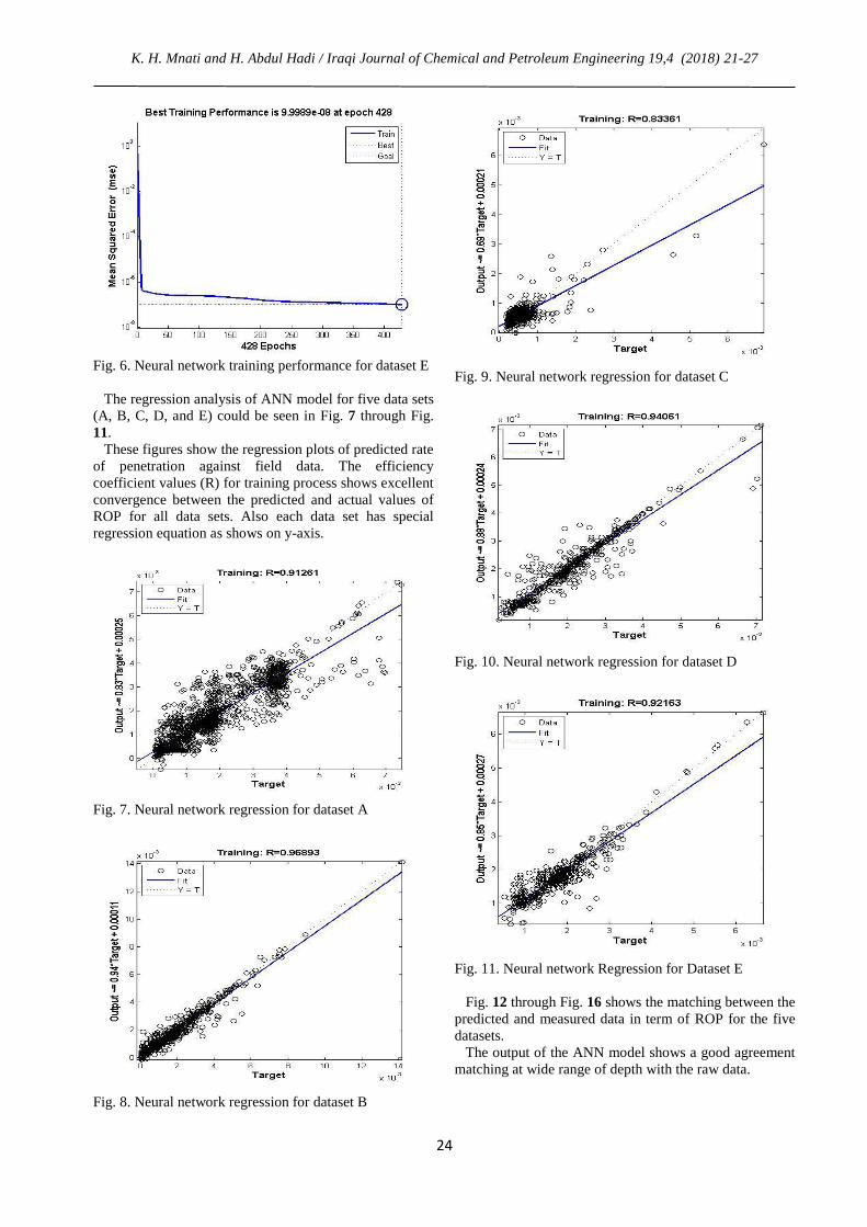
The regression analysis of ANN model for five data sets

(A, B, C, D, and E) could be seen in Fig. 7 through Fig.

11.

These figures show the regression plots of predicted rate

of penetration against field data. The efficiency

coefficient values (R) for training process shows excellent

convergence between the predicted and actual values of

ROP for all data sets. Also each data set has special

regression equation as shows on y-axis.

Fig. 7. Neural network regression for dataset A

Fig. 8. Neural network regression for dataset B

Fig. 9. Neural network regression for dataset C

Fig. 10. Neural network regression for dataset D

Fig. 11. Neural network Regression for Dataset E

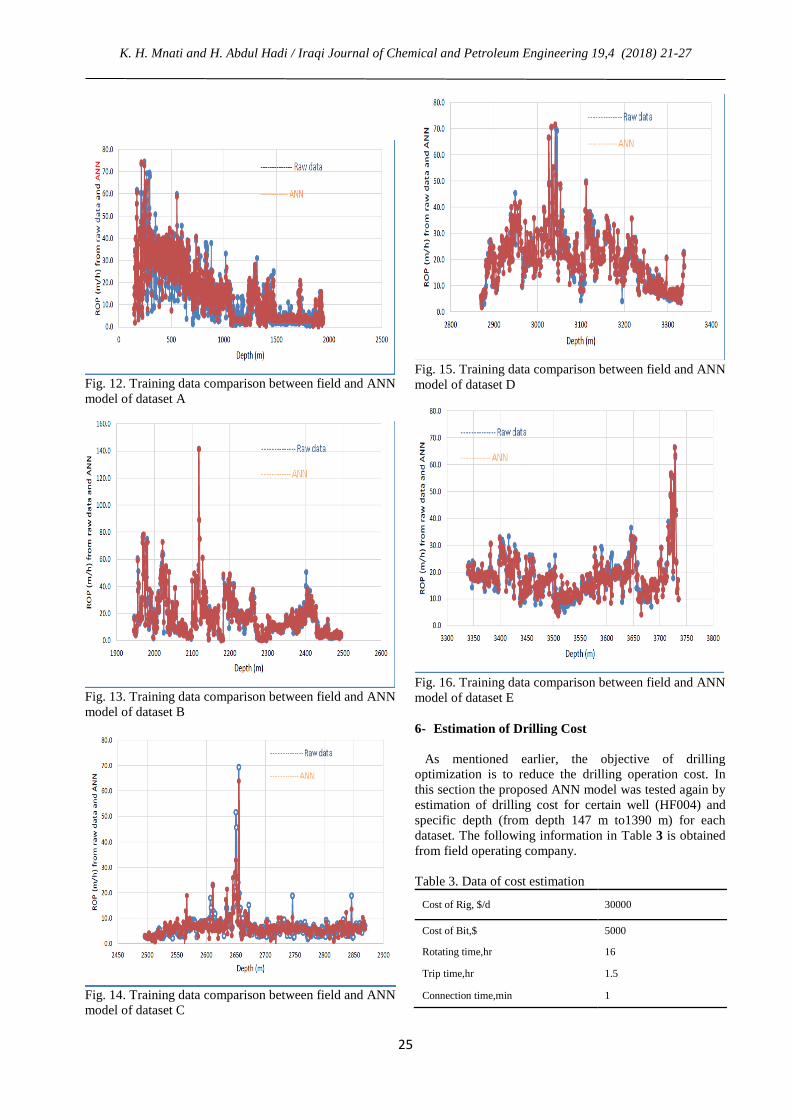
Fig. 12 through Fig. 16 shows the matching between the

predicted and measured data in term of ROP for the five

datasets.

The output of the ANN model shows a good agreement

matching at wide range of depth with the raw data.

K. H. Mnati and H. Abdul Hadi / Iraqi Journal of Chemical and Petroleum Engineering 19,4 (2018) 21-27

22

Fig. 12. Training data comparison between field and ANN

model of dataset A

Fig. 13. Training data comparison between field and ANN

model of dataset B

Fig. 14. Training data comparison between field and ANN

model of dataset C

Fig. 15. Training data comparison between field and ANN

model of dataset D

Fig. 16. Training data comparison between field and ANN

model of dataset E

6- Estimation of Drilling Cost

As mentioned earlier, the objective of drilling

optimization is to reduce the drilling operation cost. In

this section the proposed ANN model was tested again by

estimation of drilling cost for certain well (HF004) and

specific depth (from depth 147 m to1390 m) for each

dataset. The following information in Table 3 is obtained

from field operating company.

Table 3. Data of cost estimation

Cost of Rig, $/d 30000

Cost of Bit,$ 5000

Rotating time,hr 16

Trip time,hr 1.5

Connection time,min 1

K. H. Mnati and H. Abdul Hadi / Iraqi Journal of Chemical and Petroleum Engineering 19,4 (2018) 21-27

22

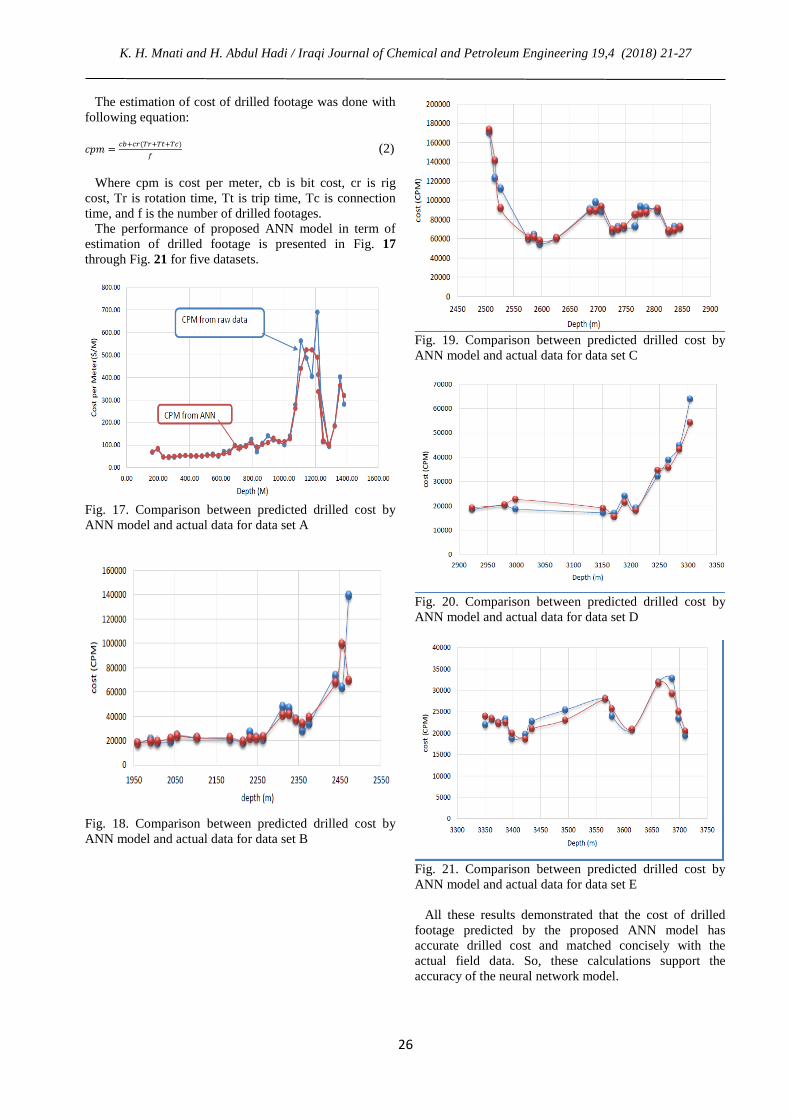
The estimation of cost of drilled footage was done with

following equation:

(2)

Where cpm is cost per meter, cb is bit cost, cr is rig

cost, Tr is rotation time, Tt is trip time, Tc is connection

time, and f is the number of drilled footages.

The performance of proposed ANN model in term of

estimation of drilled footage is presented in Fig. 17

through Fig. 21 for five datasets.

Fig. 17. Comparison between predicted drilled cost by

ANN model and actual data for data set A

Fig. 18. Comparison between predicted drilled cost by

ANN model and actual data for data set B

Fig. 19. Comparison between predicted drilled cost by

ANN model and actual data for data set C

Fig. 20. Comparison between predicted drilled cost by

ANN model and actual data for data set D

Fig. 21. Comparison between predicted drilled cost by

ANN model and actual data for data set E

All these results demonstrated that the cost of drilled

footage predicted by the proposed ANN model has

accurate drilled cost and matched concisely with the

actual field data. So, these calculations support the

accuracy of the neural network model.

K. H. Mnati and H. Abdul Hadi / Iraqi Journal of Chemical and Petroleum Engineering 19,4 (2018) 21-27

22

7- Conclusions

Based on the previous calculation, an Artificial Neural

Network model of three layers for estimating rate of

penetration of Alhalfaya oil field could be constructed

with aid of five data sets from mud and wire line logs. A

large training process for each data set were conducted

due to high quantity of field data and could be obtained

high performance of ANN model by reducing the mean

square error to minimum level, and improving the value

of efficiency coefficient.

The ANN proposed model showed good feasibility and

accuracy when it applied for estimation the rate of

penetration in five formations due to high matching with

the raw data. Also, economic application of the proposed

ANN model for estimation the cost of drilled footage in

five data sets showed their capability for yielding quite

accurate outcome.

Nomenclature

Cpm: cost per meter,$/m

Cr: rig cost, $/hr

F: No of drilled meter,m

R: Efficiency coefficient

Tc: connection time,hr

Tr: rotation time, hr

Tt: trip time, hr

References

[1] Rahimzadeh,H.et al.,2010.Comparison of the

Penetration Rate Models Using Field Data for One of

the Gas Fields in Persian Gulf Area.In Proceedings of

International Oil and Gas Conference and Exhibition

in China.Society of Petroleum Engineers.

[2] Mendes,J.R.P.,FONSECA,T.C.&

SERAPIAO,A.,2007.Applying AGenetic Neurol

Model Reference Adaptive Controller in Drilling

Optimization.World Oil,228(10).

[3] Wang,F.& Salehi,S.,2015.Drilling Hydraulic

Optimization Using Neurol Networks.SPE

173420,SPE Digital Energy Conference and

Exhibition,Texas,USA,3-5 March.

[4] Bahari,M.,H. et al(2008).Determining Bourgoyne and

Young Model Coefficients Using Genetic Algorithm

to Predict Drilling Rate.Journal of Applied Science

8(17):3050-3054.

[5] Jahanbakhish,R.and Keshavarzi,R.,2012.Real-Time

Prediction of Rate of Penetration During Drilling

Operation in Oil and Gas Wells.46th

American Rock

Mechanics/Geomechanics

Symposium,Chicago,IL,USA,24-27 June.

[6] Bataee,M.& Mohseni,S.,2011.Application of Artificial

Intelligent Systems in ROP Optimization:a Case study

in Shadegan Oil Field.SPE 140029,SPE Middle East

Unconventional Gas Conference and

Exhibition,Muscat,Oman,31 January-2 February.

[7] Bontempi,G.,Bersini,H.& Birattari,M.,2001. The

Local Paradigm for modeling and Control:from

Neuro-Fuzzy Sets and Systems,121(1),pp.59-72.

الحمفاية النفطي تخمين معدل الحفر والكمفة بواسطة الشبكة العصابية الصناعية لحقل

الخلاصة

اىمية كبيرة في الحفر الامثل بسبب تاثيره المحوري عمى كمفة عمميات التخمين الدقيق لمعدل الحفر ذو الحفر. وعادة يكون ىذا التخمين صعب بسبب تداخل العوامل التي تؤثر عمى عممية الحفر.في ىذا البحث تم

,حيث تم بناء موديل الصناعية كاسموب جديد لتخمين معدل الحفر والكمفةاستخدام طريقة الشبكة العصابية الشبكة العصابية من ثلاثة طيقات اثنان مخفية وواحدة لمنواتج باستعمال بيانات مجسات الطين والمجسات

,سرعة الاخرى لحقل الحمفاية النفطي. العوامل التي تم اسخدام قيميا ىي العوامل الميكانيكية )الوزن المسمط الدوران(,العوامل الييدروليكية,وزمن انتقال الموجة الصوتية .

%من البيانات 58تم استخدام خمس مجاميع لمبيانات والتي نمثل خمس تكوينات في الحقل حيث تم استخدام موديل % لاختبار صلاحيتو. بينت النتائج التطابق الجيد لقيم معدل الحفر المحتسبة من ال58لتدريب الموديل و

مع القيم المقاسة وكذلك لقيم الكمفة المحتسبة مع القيم الاصمية.