Practical and Rigorous Uncertainty Bounds for Gaussian Process Regression

Christian Fiedler,1, 2, 3 Carsten W. Scherer,2 Sebastian Trimpe 1, 3

1Intelligent Control Systems Group, Max Planck Institute for Intelligent Systems2Mathematical Systems Theory, University of Stuttgart

3Institute for Data Science in Mechanical Engineering, RWTH Aachen Universityfiedler@is.mpg.de, carsten.scherer@imng.uni-stuttgart.de, trimpe@dsme.rwth-aachen.de

Abstract

Gaussian Process Regression is a popular nonparametric re-gression method based on Bayesian principles that providesuncertainty estimates for its predictions. However, these esti-mates are of a Bayesian nature, whereas for some importantapplications, like learning-based control with safety guaran-tees, frequentist uncertainty bounds are required. Althoughsuch rigorous bounds are available for Gaussian Processes,they are too conservative to be useful in applications. Thisoften leads practitioners to replacing these bounds by heuris-tics, thus breaking all theoretical guarantees. To address thisproblem, we introduce new uncertainty bounds that are rigor-ous, yet practically useful at the same time. In particular, thebounds can be explicitly evaluated and are much less conser-vative than state of the art results. Furthermore, we show thatcertain model misspecifications lead to only graceful degra-dation. We demonstrate these advantages and the usefulnessof our results for learning-based control with numerical ex-amples.

1 IntroductionGaussian Processes Regression (GPR) is an establishedand successful nonparametric regression method based onBayesian principles (Rasmussen and Williams 2006) whichhas recently become popular in learning-based control (Liuet al. 2018; Kocijan 2016). In this context, safety and perfor-mance guarantees are important aspects (Astrom and Mur-ray 2010; Skogestad and Postlethwaite 2007). In fact, thelack of rigorous guarantees has been identified as one of themajor obstacles preventing the usage of learning-based con-trol methodologies in safety-critical areas like autonomousdriving, human-robot interaction or medical devices, see e.g.(Berkenkamp 2019). One approach to tackle this challengeis to use the posterior variance of GPR to derive frequentistuncertainty bounds and combine these with robust controlmethods that can deal with the remaining uncertainty. Thisstrategy has been successfully applied in a number of worksthat also provide control-theoretical guarantees, cf. Section2.2.

These approaches rely on rigorous frequentist uncertaintybounds for GPR. Although such results are available (Srini-vas et al. 2010, Theorem 6), (Chowdhury and Gopalan

Copyright © 2021, Association for the Advancement of ArtificialIntelligence (www.aaai.org). All rights reserved.

2017, Theorem 2), they turn out to be very conservativeand difficult to evaluate numerically in practice and are,hence, replaced by heuristics. That is, instead of bounds ob-tained from theory, much smaller ones are assumed, some-times without any practical justification, cf. Section 2.3 formore discussion. Unfortunately, using heuristic approxima-tions leads to a breakdown of the theoretical guarantees ofthese control approaches, as already observed for examplein (Lederer, Umlauft, and Hirche 2019). Furthermore, whenderiving theoretical guarantees based on frequentist resultslike (Srinivas et al. 2010, Theorem 6) or (Chowdhury andGopalan 2017, Theorem 2), model misspecifications (likewrong hyperparameters of the underlying GPR model or ap-proximations such as the usage of sparse GPs) are ignored.Since model misspecifications are to be expected in any real-istic setting, the validity of such theoretical guarantees basedon idealized assumptions is unclear.

In summary, rigorous and practical frequentist uncertaintybounds for GPR are currently not available. By practicalwe mean that concrete, not excessively conservative nu-merical bounds can be computed based on reasonable andestablished assumptions and that these are robust againstmodel misspecifications at least to some extent. We notethat such bounds are of independent interest, for example,for Bayesian Optimization (Shahriari et al. 2015). In thiswork, we improve previous frequentist uncertainty boundsfor GPR leading to practical, yet theoretically sound re-sults. In particular, our bounds can be directly used in al-gorithms and are sharp enough to avoid the use of unjusti-fied heuristics. Furthermore, we provide robustness resultsthat can handle moderate model misspecifications. Numer-ical experiments support our theoretical findings and illus-trate the practical use of the bounds.

2 Background2.1 Gaussian Process Regression and

Reproducing Kernel Hilbert SpacesWe briefly recall the basics of GPR, for more details werefer to (Rasmussen and Williams 2006). A Gaussian Pro-cess (GP) over an (input or index) set D is a collectionof random variables, such that any finite subset is nor-mally distributed. A GP f is uniquely determined by itsmean function m(x) = E[f(x)] and covariance function

arX

iv:2

105.

0279

6v1

[cs

.LG

] 6

May

202

1

k(x, x′) = E[(f(x)−m(x))(f(x′)−m(x′))] and we writef ∼ GD(m, k). Without loss of generality we focus onthe case m ≡ 0. Common covariance functions includethe Squared Exponential (SE) and Matern kernel. Considera Gaussian Process prior f ∼ GD(0, k) and noisy data(xi, yi)i=1,...,N , where xi ∈ D and yi = f(xi) + εi withi.i.d. N (0, σ2) noise, then the posterior is also a GP, withthe posterior mean µN , posterior covariance kN and poste-rior variance given by

µN (x) = µ(x) + kN (x)T (KN + σ2IN )−1yN

kN (x, x′) = k(x, x′)− kN (x)T (KN + σ2IN )−1kN (x′)

σ2N (x) = kN (x, x),

where we defined the kernel matrix KN =(k(xj , xi))i,j=1,...,N and the column vectors kN (x) =(k(xi, x))i=1,...,N and yN = (yi)i=1,...,N .

Later on we follow (Srinivas et al. 2010; Chowdhury andGopalan 2017) and assume that the ground truth is a functionfrom a Reproducing Kernel Hilbert Space (RKHS). For anintroduction to the RKHS framework we refer to (Steinwartand Christmann 2008, Chapter 4) or (Berlinet and Thomas-Agnan 2011) as well as (Kanagawa et al. 2018) for con-nections between Gaussian Processes and the RKHS frame-work.

2.2 Bayesian and Frequentist BoundsGPR is based on Bayesian principles: A prior distribution ischosen (here a GP with given mean and covariance function)and then updated with the available data using Bayes rule,assuming a certain likelihood or noise model (here indepen-dent Gaussian noise). The updated distribution is called theposterior distribution and can be interpreted as a tradeoff be-tween prior belief (encoded in the prior distribution togetherwith the likelihood model) and evidence (the data) (Murphy2012, Chapter 5). In contrast to the Bayesian approach, infrequentist statistics the existence of a ground truth is as-sumed and noisy data about this ground truth is acquired(Murphy 2012, Chapter 6).

For many applications which require safety guarantees itis important to get reliable frequentist uncertainty bounds.A concrete setting and major motivation for this work islearning-based robust control. Here, the ground truth is anonly partially known dynamical system and the goal is tosolve a certain control task, like stabilization or tracking,by finding a suitable controller. A machine learning methodlike GPR is used to learn more about the unknown dynami-cal system from data. Thereafter a set of possible models isderived from the learning method that contains the groundtruth with a given (high) probability. For this reason sucha set is often called an uncertainty set. We then use a robustmethod on this set, i.e., a method the leads to a controller thatworks for every element of this set. Since the ground truth iscontained in this set with a given (high) probability, the taskis solved with this (high) probability. Examples of such anapproach are (Koller et al. 2018) (using robust model pre-dictive control with state constraints), (Umlauft et al. 2017)(using feedback linearization to achieve ultimate bounded-

ness) and (Helwa, Heins, and Schoellig 2019) (consideringtracking of Lagrangian systems).

The control performance typically degrades with largeruncertainty sets, and it might even be impossible to achievethe control goal if the uncertainty sets are too large (Sko-gestad and Postlethwaite 2007). Therefore it is desirable toextract uncertainty sets that are as small as possible, but stillinclude the ground truth with a given high probability. Inparticular, when using GPR, this necessitates frequentist un-certainty bounds that are not too conservative, so that theuncertainty sets are not too large. Furthermore, we also haveto be able to evaluate the uncertainty bounds numerically,since robust control methods typically need an explicit un-certainty set.

For learning-based control applications using GPR to-gether with robust control methods, bounds of the followingform have been identified as the most useful ones: Let X bean arbitrary input set and assume that f : X → R is theunknown ground truth. Let µN be the posterior mean usinga dataset of size N , generated from the ground truth, and letδ ∈ (0, 1) be given. We need a function νN (x) that can beexplicitly evaluated, such that with probability at least 1− δwith respect to the data generating process, we have

|f(x)− µN (x)| ≤ νN (x) ∀x ∈ X. (1)

We emphasize that the probability statement is with re-spect to the noise generating process, and that the under-lying ground truth is just some deterministic function. Fora more thorough discussion we refer to (Berkenkamp 2019,Section 2.5.3).

2.3 Related WorkFrequentist uncertainty bounds for GPR as considered in thiswork were originally developed in the literature on bandits.To the best of our knowledge, the first result in this direc-tion was (Srinivas et al. 2010, Theorem 6), which is of theform (1) with νN (x) = βNσN (x). Here βN is a constantthat depends on the maximum information gain, an informa-tion theoretic quantity. For common settings, there exist up-per bounds on the latter quantity, though these increase withsample size. The result from (Srinivas et al. 2010) has beensignificantly improved in (Chowdhury and Gopalan 2017,Theorem 2), though the latter still uses an upper bound de-pending on the maximum information gain. The importanceof (Srinivas et al. 2010, Theorem 6) and (Chowdhury andGopalan 2017, Theorem 2) for other applications outsidethe bandit setting has been recognized early on, in partic-ular in the control community, for example in (Berkenkamp,Schoellig, and Krause 2016; Berkenkamp et al. 2016; Kolleret al. 2018; Berkenkamp 2019; Umlauft et al. 2017; Helwa,Heins, and Schoellig 2019).

Unfortunately, both (Srinivas et al. 2010, Theorem 6)and (Chowdhury and Gopalan 2017, Theorem 2) tend tobe very conservative, especially for control applications(Berkenkamp, Schoellig, and Krause 2016; Berkenkamp2019). Furthermore, both results rely on an upper boundof the maximum information gain, which can be difficult toevaluate (Srinivas et al. 2010), though asymptotic bounds areavailable for standard kernels like the linear, SE or Matern

kernel. However, for most control applications, these asymp-totic bounds are not useful since one requires a concrete nu-merical bound in the nonasymptotic setting.

For these reasons, previous work utilizing (Srinivas et al.2010, Theorem 6) or (Chowdhury and Gopalan 2017, Theo-rem 2) used heuristics. In the control community, it is com-mon to choose a constant value βN ≡ β in an ad-hocmanner, see for example (Berkenkamp et al. 2017, 2016;Koller et al. 2018; Berkenkamp, Schoellig, and Krause2016; Helwa, Heins, and Schoellig 2019). This choice doesnot reflect the asymptotic behaviour of the scaling since themaximum information gain grows with the number of sam-ples (Srinivas et al. 2010)1. The problem with such heuristicsis that they might work in practice, but all theoretical guaran-tees that are based on results like (Chowdhury and Gopalan2017, Theorem 2) are lost, in particular, safety guaranteeslike constraint satisfaction or certain stability notions. Thisis especially problematic since one of the major incentivesto use GPR together with such results is to provably ensureproperties like stability of a closed loop system.

Note that in concrete applications one has to make someassumptions on the ground truth at some point. However,it is not clear at all how a constant scaling β as used inthese heuristics can be derived from real-world propertiesin a principled manner. In contrast to such heuristics, in theoriginal bounds (Srinivas et al. 2010, Theorem 6), (Chowd-hury and Gopalan 2017, Theorem 2) every ingredient (i.e.,desired probability, size of noise, bound on RKHS norm) hasa clear interpretation.

It seems to be well-known in the multiarm-bandit litera-ture that, in the present situation, it is possible to use moreempirical bounds than (Chowdhury and Gopalan 2017, The-orem 2). Such approaches are conceptually similar to theresults that we will present in Section 3 below, cf. (Abbasi-Yadkori 2013) and the recent work (Calandriello et al. 2019).However, to the best of our knowledge, results like Theorem1 are rarely used in applications. In particular, it seems thatno attempts have been made in the control community to usesuch a-posteriori bounds in the GPR context.

Model misspecification in the context of GPR has beendiscussed before in some works. In (Beckers, Umlauft, andHirche 2018) a numerical method for bounding the mean-squared-error of a misspecified GP is considered, but it relieson a probabilistic setting. The recent article (Wang, Tuo, andJeff Wu 2019) provides uniform error bounds and deals withmisspecified kernels, but again uses a probabilistic settingand focuses on the noise-free case.

A work with goals similar to ours is (Lederer, Umlauft,and Hirche 2019). The authors recognize and explicitly dis-cuss some of the problems of (Chowdhury and Gopalan2017, Theorem 2) in the context of control. However, (Led-erer, Umlauft, and Hirche 2019) uses a probabilistic setting,while our work is concerned with a fixed, but unknown un-derlying target function, and hence our results are of a worst-case nature. As we argued in Section 2.2, this is the settingrequired for robust approaches. Finally, the very recent work

1Sometimes other heuristics are used that ensure that βN growswith N , cf. e.g. (Kandasamy, Schneider, and Poczos 2015)

(Maddalena, Scharnhorst, and Jones 2020) requires boundednoise and does not deal with model misspecification.

3 Practical and Rigorous FrequentistUncertainty Bounds

We now present our main technical contributions. The keyobservation is that for many applications relying on frequen-tist uncertainty bounds, in particular, learning-based controlmethods, only a-posteriori bounds are needed. This meansthat the frequentist uncertainty set can be derived after thelearning process and hence the concrete realization of thedataset can be used. We take advantage of this fact and mod-ify existing uncertainty results so that they explicitly dependon the dataset used for learning. In general no a-priori guar-antees can be derived from the results we present here, butthis does not play a role in the present setting.

The following result, which is a modified version of(Chowdhury and Gopalan 2017, Theorem 2), is fundamentalfor the rest of the paper.Theorem 1. Let D 6= ∅ be a set and k : D×D → R a pos-itive definite kernel with corresponding RKHS (Hk, ‖ · ‖k)and let f ∈ Hk with ‖f‖k ≤ B for some B ≥ 0. LetF = (Fn)n∈N be a filtration and (xn)n∈N a D-valueddiscrete-time stochastic process that is predictable w.r.t. Fand let (εn)n be an R-valued stochastic process adapted toF, such that εn conditioned on Fn−1 is R-subgaussian withR ≥ 0. Furthermore, define yn = f(xn) + εn for all n ≥ 1.

Consider a Gaussian process g ∼ GD(0, k) and denoteits posterior mean function by µN , its posterior covariancefunction by kN and its posterior variance by σ2

N (x) :=kN (x, x), w.r.t. to data (x1, y1), . . . , (xN , yN ), assumingin the likelihood independent Gaussian noise with meanzero and variance λ > 0. Then for any δ ∈ (0, 1) withλ = max{1, λ} and

βn = βn(δ,B,R, λ)

= B +R√

log(det(Kn + λIn)

)− 2 log(δ) (2)

one has

P [|µN (x)− f(x)| ≤ βNσN (x) ∀N ∈ N, x ∈ D] ≥ 1− δ.(3)

Proof. (Idea) Essentially identical to the proof of (Chowd-hury and Gopalan 2017, Theorem 2), however, we do notupper-bound (2) by the maximum information gain. Detailsare given in the supplementary material.

The key insight is that by appropriate modifications of theproof of (Chowdhury and Gopalan 2017, Theorem 2) we ob-tain a frequentist uncertainty bound for GPR that fulfills alldesiderata from Section 2.2. In the numerical examples be-low we show that the bound is often tight enough for practi-cal purposes.

Independent inputs and noise (e.g. deterministic inputsand i.i.d. noise) is a common situation that is simpler thanthe setting of Theorem 1. In this case the following a-posteriori bound can be derived that does not depend any-more on log det.

Proposition 2. Let D 6= ∅ be a set and k : D × D → Ra positive definite kernel with corresponding RKHS (Hk, ‖ ·‖k) and let f ∈ Hk with ‖f‖k ≤ B for some B ≥ 0. Letx1, . . . , xN ∈ D be given and ε1, . . . , εN be R-valued in-dependent R-subgaussian random variables. Furthermore,define yn = f(xn) + εn for all n = 1, . . . , N .

Consider a Gaussian process g ∼ GD(0, k) and denoteits posterior mean function by µN , its posterior covariancefunction by kN and its posterior variance by σ2

N (x) :=kN (x, x), w.r.t. to data (x1, y1), . . . , (xN , yN ), assuming inthe likelihood independent Gaussian noise with mean zeroand variance λ ≥ 0. Then for any δ ∈ (0, 1) with

ηN (x) = R‖(KN + λIN )−1kN (x)‖

×

√√√√N + 2√N

√log

[1

δ

]+ 2 log

[1

δ

]one has

P [|µN (x)− f(x)| ≤ BσN (x) + ηN (x) ∀x ∈ D] ≥ 1− δ.

Proof. (Idea) Similar to the proof of Theorem 1, but use(Hsu et al. 2012, Theorem 2.1) instead of (Chowdhury andGopalan 2017, Theorem 1). Details are provided in the sup-plementary material.

3.1 Using the Nominal BoundWe will now discuss how the previous bounds can be ap-plied. In particular, we will carefully examine potential dif-ficulties that have been identified in similar settings in theliterature before.

Kernel Choice and RKHS Norm Bound Theorem 1 andProposition 2 require an upper bound on the RKHS normof the target function, i.e., ‖f‖k ≤ B. In particular, the tar-get function has to be in the RKHS corresponding to thecovariance function used in GPR. Since we do not rely onbounds on the maximum information gain, very general ker-nels can be used together with Theorem 1 and Proposition2. For example, highly customized kernels can be directlyused and no derivation of additional bounds is necessary, aswould be the case for (Srinivas et al. 2010, Theorem 6) or(Chowdhury and Gopalan 2017, Theorem 2). In particular,our results support the usage of linearly constrained Gaus-sian Processes (Jidling et al. 2017; Lange-Hegermann 2018)and related approaches like (Geist and Trimpe 2020). Get-ting a large enough, yet not too conservative bound on theRKHS norm of the target function can be difficult in general.However, since the kernel encodes prior knowledge, domainknowledge could be used to arrive at such upper bounds. De-veloping general and systematic methods to transform estab-lished domain knowledge into bounds on the RKHS norm isleft for future work.

Hyperparameters As with other bounds for GPR the in-ference of hyperparameters is critical. First of all, an inspec-tion of the proof of (Chowdhury and Gopalan 2017, The-orem 2) shows that the nominal noise variance λ is inde-

pendent of the actual subgaussian noise2 (with subgaussianconstantR). In particular, Theorem 1 and Proposition 2 holdtrue for any admissible noise variance, though it is not clearwhat the optimal choice would be.

In GPR the precise specification of the covariance func-tion is usually not given. In the most common situation a cer-tain kernel class is selected, e.g. SE kernels, and the remain-ing hyperparameters, e.g. the length-scale of an SE kernel,is inferred by likelihood optimization or in a fully Bayesiansetting by using hyperpriors. In both cases the results fromabove do not directly apply since they rely on given correctkernels. Incorporating the hyperparameter inference in re-sults like Theorem 1 in a principled manner is an importantopen question for future work. As a first step into this direc-tion, we provide robustness results in Section 3.2.

Computational Complexity For many interesting appli-cations the sample sizes are small enough, so that standardGPR together with Theorem 1 can be used directly. Further-more, for control applications the GP model is often usedoffline and only derived information is used in the actualcontroller which has restricted computational resources andreal-time constraints.

There might be cases where standard GPR can be used,but the calculation of log det is prohibitive. In such a situ-ation it is possible to use powerful approximation methodsfor the latter quantity. Since quantitative approximation errorbounds are available in this situation, e.g. (Han, Malioutov,and Shin 2015; Dong et al. 2017), one can simply add acorresponding margin in the definition of βN . Additionally,in some cases the log det can be efficiently calculated, inparticular for semi-separable kernels (Andersen and Chen2020), which play an important role in system identification(Chen and Andersen 2020). Note also that the applicationof Proposition 2 does not require the computation of log detterms.

Additionally, due to the very general nature of Theorem1 any approximation approach for GPR based on subsets ofthe training data that does not update the kernel parameterscan be used and no modifications of the uncertainty boundsare necessary. In particular, the maximum variance selectionprocedure (Jain et al. 2018; Koller et al. 2018) is compatiblewith Theorem 1 and Proposition 2.

Finally, any GPR approximation method that does not up-date the kernel hyperparameters and gives quantitative ap-proximation error estimates for the posterior mean and vari-ance can be used with Theorem 1, where the respectivequantities have to be adapted according to the method used.An example of such an approximation method with error es-timates is (Huggins et al. 2019).

3.2 Bounds under Model MisspecificationAs usual in the literature, Theorem 1 and Proposition 2 usethe same kernel k for generating the RKHS containing the

2In fact λ in the corresponding (Chowdhury and Gopalan 2017,Theorem 2) has been used as a tuning parameter in (Chowdhuryand Gopalan 2017).

ground truth and as a covariance function in GPR. Obvi-ously, in practice it is unlikely that one gets the kernel of theground truth exactly right. However, it turns out that this isnot a big problem. We first note a simple, yet interesting factthat follows immediately from the proof of (Chowdhury andGopalan 2017, Theorem 2).

Proposition 3. Consider the situation of Theorem 1, but thistime assume that the ground truth f is from another RKHSH . If H ⊆ H , and the inclusion id : H → H is continu-ous with operator norm at most 1, then the result holds truewithout any modification.

This simple result can easily be used to verify that formany common situations misspecification of the kernel isnot a problem. As an example, we consider the case of thepopular isotropic SE kernel.

Proposition 4. Consider the situation of Theorem 1, but letf ∈ H , where H is the RKHS corresponding to the SE ker-nel k (on ∅ 6= D ⊆ Rd) with length scale 0 < γ. Usefor the Gaussian Process Regression the SE kernel k withlength-scale 0 < γ ≤ γ. Then Theorem 1 holds true withoutchange.

Proof. Follows immediately from Proposition 3 and (Stein-wart and Christmann 2008, Proposition 4.46).

These results tell us that it is not a problem if we do notget the hyperparameter of the isotropic SE kernel right, aslong as we underestimate the length-scale. This is intuitivelyclear since a smaller length-scale corresponds to more com-plex functions. Similar results are known in related contexts,for example (Szabo et al. 2015). Note that Proposition 4 doesnot imply that one should choose a very small length-scale.The result makes a statement on the validity of the frequen-tist uncertainty bound from Theorem 1, but not on the sizeof the uncertainty set. For a similar discussion in a slightlydifferent setting see (Wang, Tuo, and Jeff Wu 2019).

Next, we consider the question what happens when theground truth is from a different kernel k, such that the cor-responding RKHS H is not included in the RKHS H cor-responding to the covariance function k used in the GPR.Intuitively, since the functions in an RKHS are built fromthe corresponding reproducing kernel, cf. e.g. (Steinwart andChristmann 2008, Theorem 4.21), Theorem 1 should holdapproximately true if the kernels k and k are not too differ-ent. This is made precise in the following result. Its proof isprovided in the supplementary material.

Theorem 5. Consider the situation of Theorem 1 but thistime assume that the target function f is from the RKHS(H, ‖ · ‖k) of a different kernel k such that still ‖f‖k ≤ B

and supx,x′∈D |k(x, x′)− k(x, x′)| ≤ ε for some ε ≥ 0. Wethen have for any δ ∈ (0, 1) that

P [|µN (x)− f(x)| ≤ νN (x) ∀N ∈ N, x ∈ D] ≥ 1− δ

where

νN (x) = βN (δ)√σ2N (x) + S2

N (x) + CN (x)‖yN‖,

and βN (δ) = βN (δ,B,R, λ+Nε) as in Theorem 1 and

S2N (x) = ε+

√Nε‖(KN + λIN )−1kN (x)‖

+ (√Nε+ ‖kN (x)‖)CN (x) (4)

CN (x) =

(1

λ+ ‖(KN + λIN )−1‖

)(‖kN (x)‖+

√Nε)

+ ‖(KN − λIN )−1‖√Nε (5)

We can interpret Theorem 5 as a robust version (w.r.t. dis-turbance of the kernel) of Theorem 1. By using the boundsfrom Theorem 5 we can ensure that the resulting uncertaintyset contains the ground truth with prescribed probability de-spite using the wrong kernel.

In Theorem 1 we have a tube around µN (x) of widthβN (δ,B,R, λ)σN (x), whereas in Theorem 5 we have a tubearound µN (x) of width

βN (δ,B,R, λ+Nε)√σ2N (x) + S2

N (x) + CN (x)‖yN‖

Because of the uncertainty or disturbance in the kernel wehave to increase the nominal noise variance (used in thenominal noise model in GPR) from λ to λ + Nε, increasethe nominal posterior standard deviation from σN (x) to√σ2N (x) + S2

N (x) and add an offset to the width of the tubeof CN (x)‖yN‖. In particular, the uncertainty set now de-pends on the measured values yN . Note that CN (x) andSN (x) depend on the input, but if necessary this depen-dence can be easily removed by finding an upper boundon ‖kN (x)‖. An interesting observation is that even ifσN (x) = 0, the width of the tube around µN (x) has nonzerowidth. Intuitively this is clear since in general it can happenthat f 6∈ H , but µN ∈ H by construction. Finally, a robustversion of Proposition 2 can be derived similarly to Theorem5, see the supplementary material.

4 Numerical ExperimentsWe now test the theoretical results in numerical experimentsusing synthetic data, where the ground truth is known. First,we investigate the frequentist behaviour of the uncertaintybounds. The general setup consists of generating a func-tion from an RKHS with known RKHS norm (the groundtruth), sampling a finite data set, running GPR on this dataset and then evaluating our uncertainty bounds. This learn-ing process is then repeated on many sampled data setsand we check how often the uncertainty bounds are vio-lated. To the best of our knowledge, these types of experi-ments have actually not been done before, since usually onlythe final algorithms using the uncertainty bounds have beentested, e.g. in (Srinivas et al. 2010; Chowdhury and Gopalan2017), or no ground truth from an RKHS has been used, cf.(Berkenkamp 2019). Furthermore, we would like to remarkthat the method for generating the ground truth can resultin misleading judgements of the theoretical result. The latterhas to hold for all ground truths, but the generating methodcan introduce a bias, e.g. only generating functions of a cer-tain shape. To the best of our knowledge, this issue has notbeen pointed out before.

Second, we demonstrate the practicality and usefulness ofour uncertainty bounds by applying them to concrete exam-ple from robust control.

4.1 Frequentist Behavior of Uncertainty BoundsSetup of the Experiments Unless noted otherwise, foreach of the following experiments we use D = [−1, 1] asinput space and generate randomly 50 functions (the groundtruths) from an RKHS and evaluate these on a grid 1000equidistant points from D. We generate the functions byrandomly selecting a number of center points x ∈ D andform a linear combination of kernel functions k(·, x), wherek is the kernel of the RKHS. Additionally, for the SE ker-nel we use the orthonormal basis (ONB) from (Steinwartand Christmann 2008, Section 4.4) with random, normallydistributed coefficients to generate functions from the corre-sponding RKHS. For each function we repeat the followinglearning instance 10000 times: We sample uniformly 50 in-puts, evaluate the ground truth on these inputs and addingnormal zero-mean i.i.d. noise with standard deviation (SD)0.5. We then run GPR on each of the training sets, com-pute the uncertainty sets (for Theorem 1 this correspondsto the scaling β50) and check (on the equidistant grid ofD) whether the resulting uncertainty set contains the groundtruth.

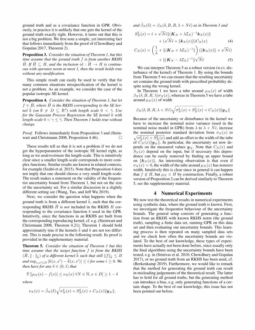
Nominal Setting Consider the case that the covariancefunction used in GPR and the kernel corresponding to theRKHS of the target function coincide. First, we test the nom-inal bound from Theorem 1 with SE and Matern kernels,respectively, for δ = 0.1, 0.01, 0.001, 0.0001. The resultingscalings β50 are shown in Table 1. As can be seen there, thescalings are reasonably small, roughly in the range of heuris-tics used in the literature, cf. (Berkenkamp 2019). Further-more, the graph of the target function is fully included in theuncertainty set in all repetitions. This is illustrated in Fig-ure 1 (LEFT), where an example instance of this experimentis shown. As can be clearly seen there, the posterior mean(blue solid line) is well within the uncertainty set from The-orem 1 (with δ = 0.01), which is not overly conservative.

Misspecified Setting We now consider misspecificationof the kernel, i.e. different kernels are used for generatingthe ground truth and as prior covariance function in GPR.As an example we use the SE kernel with different length-scales and use the ONB from (Steinwart and Christmann2008, Section 4.4) to generate the RKHS functions. We startwith the benign setting from Proposition 3, where the RKHScorresponding to the covariance function used in GPR con-tains the RKHS of the target function. For this, identical set-tings as in our first experiment above are used, but now wegenerate functions from the SE kernel with length-scale 0.5and use the SE kernel with length-scale 0.2 in GPR. Thiscorresponds to the benign setting according to Proposition4. As expected, we find the same results as above, i.e. theuncertainty set fully contains the ground truth in all repeti-tions. Furthermore, the scalings β50 are roughly of the same

Figure 1: LEFT (Nominal setting): Example function(green) from SE kernel with length-scale 0.5 and RKHSnorm 2, learned from 50 samples (red). Shown is the pos-terior mean (blue) and the uncertainty set from Theorem 1for δ = 0.01. RIGHT (Misspecified setting): Example func-tion from SE kernel with length-scale 0.2, learned with GPRusing SE covariance function with length-scale 0.5. The vi-olation of the uncertainty set is clearly visible.

Table 1: β50 in nominal setting (mean ± standard deviationover all repetitions)

δ 0.1 0.01 0.001 0.0001SE 4.20± 0.02 4.45± 0.01 4.67± 0.01 4.88± 0.01

Matern 4.33± 0.02 4.57± 0.02 4.78± 0.01 4.98± 0.01

size as in the nominal case, cf. Table 2 (upper row).Next, we investigate the problematic setting where the

RKHS corresponding to the covariance function used inGPR does not contain the RKHS of the target function any-more. As an example we use again the SE kernel, but nowwith length-scale 0.2 for generating RKHS functions and theSE kernel with length-scale 0.5 for GPR. We found a con-siderable number of function instances where the boundsfrom Theorem 1 were violated with higher frequency thanδ. More precisely, for a given function the tube of widthβ50σ50(x) around µ50(x) does not fully contain the func-tion in more than δ × 10000 of the learning instances. Thishappened for 2, 6, 12, 13 out of 50 functions for δ =0.1, 0.01, 0.001, 0.0001, respectively.

Interestingly, when performing this experiment using thestandard approach of generating functions from the RKHSbased on linear combinations of kernels, we did not findfunctions that violated the uncertainty bounds more oftenthan prescribed. This reaffirmes our introductory remark thatthe method generating the test targets can lead to wrongjudgements of the theoretical results.

The results of the previous two experiments indicate thata model misspecification of the kernel can be a problem anda robust result like Theorem 5 is necessary. Indeed, a rep-etition of the last experiment with the uncertainty set fromTheorem 5 instead of Theorem 1 resulted in all functionsbeing contained in the uncertainty set in all repetitions. Aninspection of the average uncertainty set widths in Table 3indicates some conservatism.

4.2 Control ExampleWe now show the usefulness of our results for robust controlby applying it to a concrete, existing learning-based controlmethod. Due to space constraints only a brief description of

Table 2: β50 in the misspecified setting (mean ± standarddeviation over all repetitions)

δ 0.1 0.01 0.001 0.0001Benign 4.20± 0.02 4.45± 0.01 4.67± 0.01 4.88± 0.01

Problematic 3.88± 0.01 4.16± 0.01 4.41± 0.01 4.64± 0.01

Table 3: Width of robust uncertainty set (mean ± SD of av-erage width)

δ 0.1 0.01 0.001 0.0001Mean 94.99± 5.61 95.84± 5.61 96.67± 5.61 97.49± 5.61

SD 8.38± 2.16 8.46± 2.17 8.53± 2.19 8.61± 2.21

the example can be given here. For more details and discus-sions we refer to the supplementary material.

As an example, we choose the algorithm from (Solopertoet al. 2018) which is a learning-based Robust Model Pre-dictive Control (RMPC) approach that comes with rigorouscontrol-theoretic guarantees. We refer to (Rawlings, Mayne,and Diehl 2017, Chapter 3) for background on RMPC and to(Hewing et al. 2019) for a recent survey on related learning-based control methods. We follow (Soloperto et al. 2018)and consider the discrete-time system[x+1x+2

]=

[0.995 0.095−0.095 0.900

] [x1x2

]+

[0.0480.95

]u+

[0

−r(x2)

](6)

modelling a mass-spring-damper system with some nonlin-earity r (this could be interpreted as a friction term). Thegoal is the stabilization of the origin subject to the stateand control constraints X = [−10, 10] × [−10, 10] andU = [−3, 3], as well as minimizing a quadratic cost.

The approach from (Soloperto et al. 2018) performs thistask by interpreting (13) as a linear system with disturbance,given by the nonlinearity r, whose graph is a-priori knownto lie in the set W0 = [−10, 10] × [−7, 7]. The nonlinear-ity is assumed to be unknown and has to be learned fromdata. The RMPC algorithm requires as an input disturbancesets W(x) such that (0 −r(x2))

> ∈ W(x) for all x ∈ X,which are in turn used to generate tightened nominal con-straints ensuring robust constraint satisfaction. Furthermore,the tighter the sets W(x) are, the better is the performanceof the algorithm. We now randomly generate the function r(which will be our ground truth) from the RKHS with ker-nel k(x, x′) = 4 exp

(− (x−x′)2

2×0.82

)with RKHS norm 2. Fol-

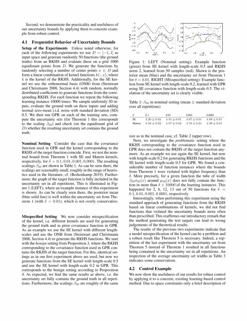
lowing (Soloperto et al. 2018), we uniformly sample 100partial states x2 ∈ [−10, 10], evaluate r at these and addi.i.d. Gaussian noise with a standard deviation of 0.01 toit. The unknown function is then learned using GPR fromthis data set. Our results then lead to an uncertainty set ofthe form W(x) = [µ100(x2) − β100σ100(x2), µ100(x2) +β100σ100(x2)], with β100 from Theorem 1 for δ := 0.001.In particular, with probability at least 1−δ we can guaranteethat r(x2) ∈ W(x) holds for all x ∈ X. Figure 2 shows theresulting tightened state constraints for an MPC horizon of9. Clearly, the state constraint sets from the learned uncer-tainty sets are much larger. Furthermore, in contrast to previ-ous work, we can guarantee that the RMPC controller using

Figure 2: Tightened state constraint sets Zk for k = 0, . . . , 9.Computed from a-priori uncertainty set W0 (LEFT) andlearned uncertainty sets W(x) (RIGHT).

these tightened state constraints retains all control-theoreticguarantees with probability at least 1−δ. In the present casewe can ensure state and control constraint satisfaction, input-to-state stability and convergence to a neighborhood of theorigin, with probability at least 1 − δ. This follows imme-diately from (Soloperto et al. 2018, Theorem 1), since theground truth r is covered by the uncertainty sets W(x) withthis probability. Note that no changes to the existing RMPCscheme were necessary and the control-theoretic guaranteeswere retained with prescribed high probability.

5 ConclusionWe discussed the importance of frequentist uncertaintybounds for Gaussian Process Regression and improved ex-isting results in this kind. By aiming only at a-posterioribounds we were able to provide rigorous and practical un-certainty results. Our bounds can be explicitly evaluatedand are sharp enough to be useful for concrete applications,as demonstrated with numerical experiments. Furthermore,we also introduced robust versions that work despite cer-tain model mismatches, which is an important concern inreal-world applications. We see the present work as a start-ing point for further developments, in particular, domain-specific versions of our results and more specific and lessconservative robustness results.

Acknowledgments. We would like to thank Sayak RayChowdhury and Tobias Holicki for helpful discussions,Steve Heim for useful comments on a draft of this work,and Raffaele Soloperto for providing the Matlab code from(Soloperto et al. 2018). Furthermore, we would like to thankthe reviewers for their helpful and constructive feedback.Funded by Deutsche Forschungsgemeinschaft (DFG, Ger-man Research Foundation) under Germany’s ExcellenceStrategy - EXC 2075 – 390740016 and in part by the Cy-ber Valley Initiative. We acknowledge the support by theStuttgart Center for Simulation Science (SimTech).

ReferencesAbbasi-Yadkori, Y. 2013. Online learning for linearlyparametrized control problems. Ph.D. thesis, University ofAlberta.

Andersen, M. S.; and Chen, T. 2020. Smoothing Splinesand Rank Structured Matrices: Revisiting the Spline Kernel.SIAM Journal on Matrix Analysis and Applications 41(2):389–412.

Astrom, K. J.; and Murray, R. M. 2010. Feedback systems:an introduction for scientists and engineers. Princeton uni-versity press.

Beckers, T.; Umlauft, J.; and Hirche, S. 2018. Mean squareprediction error of misspecified Gaussian process models.In 2018 IEEE Conference on Decision and Control (CDC),1162–1167. IEEE.

Berkenkamp, F. 2019. Safe Exploration in ReinforcementLearning: Theory and Applications in Robotics. Ph.D. the-sis, ETH Zurich.

Berkenkamp, F.; Moriconi, R.; Schoellig, A. P.; and Krause,A. 2016. Safe learning of regions of attraction for uncertain,nonlinear systems with gaussian processes. In 2016 IEEE55th Conference on Decision and Control (CDC), 4661–4666. IEEE.

Berkenkamp, F.; Schoellig, A. P.; and Krause, A. 2016. Safecontroller optimization for quadrotors with Gaussian pro-cesses. In 2016 IEEE International Conference on Roboticsand Automation (ICRA), 491–496. IEEE.

Berkenkamp, F.; Turchetta, M.; Schoellig, A.; and Krause,A. 2017. Safe model-based reinforcement learning with sta-bility guarantees. In Advances in neural information pro-cessing systems, 908–918.

Berlinet, A.; and Thomas-Agnan, C. 2011. Reproducing ker-nel Hilbert spaces in probability and statistics. Springer Sci-ence & Business Media.

Calandriello, D.; Carratino, L.; Lazaric, A.; Valko, M.; andRosasco, L. 2019. Gaussian Process Optimization withAdaptive Sketching: Scalable and No Regret. In Conferenceon Learning Theory, 533–557.

Chen, T.; and Andersen, M. 2020. On Semiseparable Ker-nels and Efficient Computation of Regularized System Iden-tification and Function Estimation. IFAC-V 2020 .

Chowdhury, S. R.; and Gopalan, A. 2017. On KernelizedMulti-armed Bandits. In International Conference on Ma-chine Learning, 844–853.

Dong, K.; Eriksson, D.; Nickisch, H.; Bindel, D.; and Wil-son, A. G. 2017. Scalable log determinants for Gaussianprocess kernel learning. In Advances in Neural InformationProcessing Systems, 6327–6337.

Geist, A. R.; and Trimpe, S. 2020. Learning Constrained Dy-namics with Gauss Principle adhering Gaussian Processes.In Proceedings of the 2nd Conference on Learning for Dy-namics and Control, 225–234.

Han, I.; Malioutov, D.; and Shin, J. 2015. Large-scale log-determinant computation through stochastic Chebyshev ex-pansions. In International Conference on Machine Learn-ing, 908–917.

Helwa, M. K.; Heins, A.; and Schoellig, A. P. 2019.Provably robust learning-based approach for high-accuracy

tracking control of lagrangian systems. IEEE Robotics andAutomation Letters 4(2): 1587–1594.Hewing, L.; Wabersich, K. P.; Menner, M.; and Zeilinger,M. N. 2019. Learning-Based Model Predictive Control: To-ward Safe Learning in Control. Annual Review of Control,Robotics, and Autonomous Systems 3.Hsu, D.; Kakade, S.; Zhang, T.; et al. 2012. A tail inequalityfor quadratic forms of subgaussian random vectors. Elec-tronic Communications in Probability 17.Huggins, J. H.; Campbell, T.; Kasprzak, M.; and Broderick,T. 2019. Scalable Gaussian Process Inference with Finite-data Mean and Variance Guarantees. In The 22nd Inter-national Conference on Artificial Intelligence and Statistics,796–805.Jain, A.; Nghiem, T.; Morari, M.; and Mangharam, R. 2018.Learning and control using Gaussian processes. In 2018ACM/IEEE 9th International Conference on Cyber-PhysicalSystems (ICCPS), 140–149. IEEE.Jidling, C.; Wahlstrom, N.; Wills, A.; and Schon, T. B. 2017.Linearly constrained Gaussian processes. In Advances inNeural Information Processing Systems, 1215–1224.Kanagawa, M.; Hennig, P.; Sejdinovic, D.; and Sriperum-budur, B. K. 2018. Gaussian processes and kernel methods:A review on connections and equivalences. arXiv preprintarXiv:1807.02582 .Kandasamy, K.; Schneider, J.; and Poczos, B. 2015. Highdimensional Bayesian optimisation and bandits via additivemodels. In International Conference on Machine Learning,295–304.Kocijan, J. 2016. Modelling and control of dynamic systemsusing Gaussian process models. Springer.Koller, T.; Berkenkamp, F.; Turchetta, M.; and Krause, A.2018. Learning-based model predictive control for safe ex-ploration. In 2018 IEEE Conference on Decision and Con-trol (CDC), 6059–6066. IEEE.Lange-Hegermann, M. 2018. Algorithmic linearly con-strained Gaussian processes. In Advances in Neural Infor-mation Processing Systems, 2137–2148.Lederer, A.; Umlauft, J.; and Hirche, S. 2019. Uniform Er-ror Bounds for Gaussian Process Regression with Applica-tion to Safe Control. In Advances in Neural InformationProcessing Systems, 657–667.Liu, M.; Chowdhary, G.; Da Silva, B. C.; Liu, S.-Y.; andHow, J. P. 2018. Gaussian processes for learning and control:A tutorial with examples. IEEE Control Systems Magazine38(5): 53–86.Maddalena, E. T.; Scharnhorst, P.; and Jones, C. N.2020. Deterministic error bounds for kernel-based learn-ing techniques under bounded noise. arXiv preprintarXiv:2008.04005 .Murphy, K. P. 2012. Machine learning: a probabilistic per-spective. MIT press.Rasmussen, C. E.; and Williams, C. K. 2006. Gaussian Pro-cesses for Machine Learning. The MIT Press.

Rawlings, J. B.; Mayne, D. Q.; and Diehl, M. 2017. Modelpredictive control: theory, computation, and design, vol-ume 2. Nob Hill Publishing Madison, WI.Shahriari, B.; Swersky, K.; Wang, Z.; Adams, R. P.; andDe Freitas, N. 2015. Taking the human out of the loop: Areview of Bayesian optimization. Proceedings of the IEEE104(1): 148–175.Skogestad, S.; and Postlethwaite, I. 2007. Multivariablefeedback control: analysis and design, volume 2. Wiley NewYork.Soloperto, R.; Muller, M. A.; Trimpe, S.; and Allgower, F.2018. Learning-based robust model predictive control withstate-dependent uncertainty. IFAC-PapersOnLine 51(20):442–447.Srinivas, N.; Krause, A.; Kakade, S.; and Seeger, M. 2010.Gaussian process optimization in the bandit setting: no re-gret and experimental design. In Proceedings of the 27th In-ternational Conference on International Conference on Ma-chine Learning, 1015–1022.Steinwart, I.; and Christmann, A. 2008. Support vector ma-chines. Springer Science & Business Media.Szabo, B.; Van Der Vaart, A. W.; van Zanten, J.; et al. 2015.Frequentist coverage of adaptive nonparametric Bayesiancredible sets. The Annals of Statistics 43(4): 1391–1428.Umlauft, J.; Beckers, T.; Kimmel, M.; and Hirche, S. 2017.Feedback linearization using Gaussian processes. In 2017IEEE 56th Annual Conference on Decision and Control(CDC), 5249–5255. IEEE.Wang, W.; Tuo, R.; and Jeff Wu, C. 2019. On predictionproperties of kriging: Uniform error bounds and robustness.Journal of the American Statistical Association 1–27.

Supplementary materialIn this supplementary material, we provide the detailed proofs in Section B that were omitted in the main paper, and furtherdetails on the numerical examples in Section B Before, we provide a straightforward and illustrative introduction to our resultsand their use in Section A3.

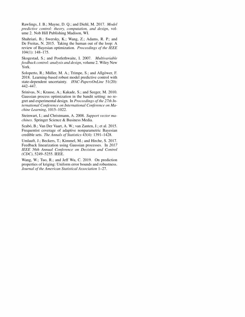
A A user-friendly overviewWe provide in this section a simple tutorial overview of the approach. For simplicity, consider a scalar function on D =[−10, 10], generated from the RKHS of the Squared Exponential (SE) kernel with RKHS norm 2. A typical example looks asfollows.

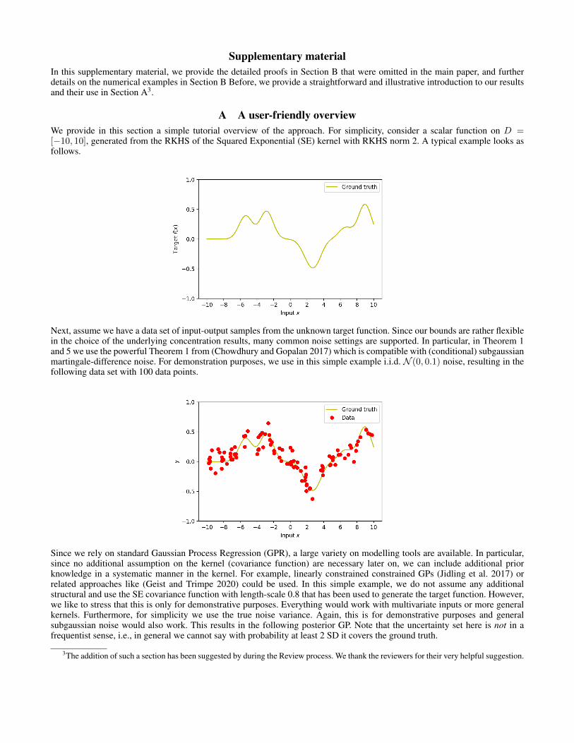
Next, assume we have a data set of input-output samples from the unknown target function. Since our bounds are rather flexiblein the choice of the underlying concentration results, many common noise settings are supported. In particular, in Theorem 1and 5 we use the powerful Theorem 1 from (Chowdhury and Gopalan 2017) which is compatible with (conditional) subgaussianmartingale-difference noise. For demonstration purposes, we use in this simple example i.i.d. N (0, 0.1) noise, resulting in thefollowing data set with 100 data points.

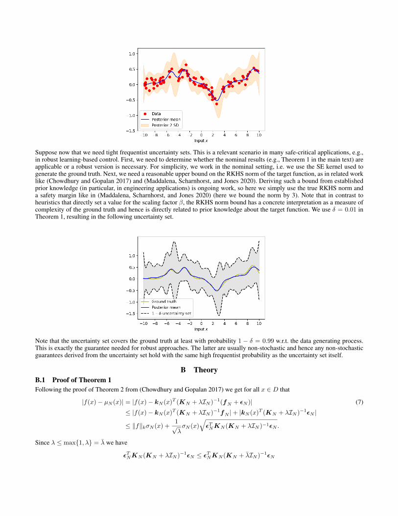
Since we rely on standard Gaussian Process Regression (GPR), a large variety on modelling tools are available. In particular,since no additional assumption on the kernel (covariance function) are necessary later on, we can include additional priorknowledge in a systematic manner in the kernel. For example, linearly constrained constrained GPs (Jidling et al. 2017) orrelated approaches like (Geist and Trimpe 2020) could be used. In this simple example, we do not assume any additionalstructural and use the SE covariance function with length-scale 0.8 that has been used to generate the target function. However,we like to stress that this is only for demonstrative purposes. Everything would work with multivariate inputs or more generalkernels. Furthermore, for simplicity we use the true noise variance. Again, this is for demonstrative purposes and generalsubgaussian noise would also work. This results in the following posterior GP. Note that the uncertainty set here is not in afrequentist sense, i.e., in general we cannot say with probability at least 2 SD it covers the ground truth.

3The addition of such a section has been suggested by during the Review process. We thank the reviewers for their very helpful suggestion.

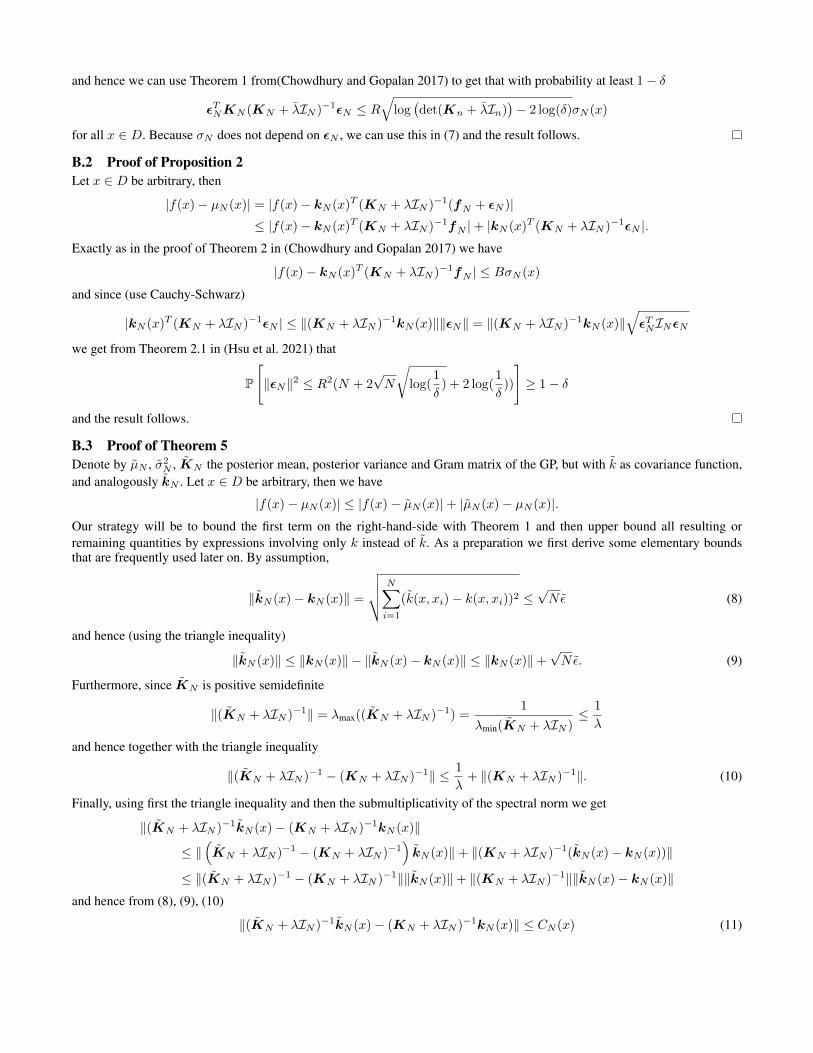
Suppose now that we need tight frequentist uncertainty sets. This is a relevant scenario in many safe-critical applications, e.g.,in robust learning-based control. First, we need to determine whether the nominal results (e.g., Theorem 1 in the main text) areapplicable or a robust version is necessary. For simplicity, we work in the nominal setting, i.e. we use the SE kernel used togenerate the ground truth. Next, we need a reasonable upper bound on the RKHS norm of the target function, as in related worklike (Chowdhury and Gopalan 2017) and (Maddalena, Scharnhorst, and Jones 2020). Deriving such a bound from establishedprior knowledge (in particular, in engineering applications) is ongoing work, so here we simply use the true RKHS norm anda safety margin like in (Maddalena, Scharnhorst, and Jones 2020) (here we bound the norm by 3). Note that in contrast toheuristics that directly set a value for the scaling factor β, the RKHS norm bound has a concrete interpretation as a measure ofcomplexity of the ground truth and hence is directly related to prior knowledge about the target function. We use δ = 0.01 inTheorem 1, resulting in the following uncertainty set.

Note that the uncertainty set covers the ground truth at least with probability 1 − δ = 0.99 w.r.t. the data generating process.This is exactly the guarantee needed for robust approaches. The latter are usually non-stochastic and hence any non-stochasticguarantees derived from the uncertainty set hold with the same high frequentist probability as the uncertainty set itself.

B TheoryB.1 Proof of Theorem 1Following the proof of Theorem 2 from (Chowdhury and Gopalan 2017) we get for all x ∈ D that

|f(x)− µN (x)| = |f(x)− kN (x)T (KN + λIN )−1(fN + εN )| (7)

≤ |f(x)− kN (x)T (KN + λIN )−1fN |+ |kN (x)T (KN + λIN )−1εN |

≤ ‖f‖kσN (x) +1√λσN (x)

√εTNKN (KN + λIN )−1εN .

Since λ ≤ max{1, λ} = λ we have

εTNKN (KN + λIN )−1εN ≤ εTNKN (KN + λIN )−1εN

and hence we can use Theorem 1 from(Chowdhury and Gopalan 2017) to get that with probability at least 1− δ

εTNKN (KN + λIN )−1εN ≤ R√

log(det(Kn + λIn)

)− 2 log(δ)σN (x)

for all x ∈ D. Because σN does not depend on εN , we can use this in (7) and the result follows.

B.2 Proof of Proposition 2Let x ∈ D be arbitrary, then

|f(x)− µN (x)| = |f(x)− kN (x)T (KN + λIN )−1(fN + εN )|≤ |f(x)− kN (x)T (KN + λIN )−1fN |+ |kN (x)T (KN + λIN )−1εN |.

Exactly as in the proof of Theorem 2 in (Chowdhury and Gopalan 2017) we have

|f(x)− kN (x)T (KN + λIN )−1fN | ≤ BσN (x)

and since (use Cauchy-Schwarz)

|kN (x)T (KN + λIN )−1εN | ≤ ‖(KN + λIN )−1kN (x)‖‖εN‖ = ‖(KN + λIN )−1kN (x)‖√εTNINεN

we get from Theorem 2.1 in (Hsu et al. 2021) that

P

[‖εN‖2 ≤ R2(N + 2

√N

√log(

1

δ) + 2 log(

1

δ))

]≥ 1− δ

and the result follows.

B.3 Proof of Theorem 5Denote by µN , σ2

N , KN the posterior mean, posterior variance and Gram matrix of the GP, but with k as covariance function,and analogously kN . Let x ∈ D be arbitrary, then we have

|f(x)− µN (x)| ≤ |f(x)− µN (x)|+ |µN (x)− µN (x)|.Our strategy will be to bound the first term on the right-hand-side with Theorem 1 and then upper bound all resulting orremaining quantities by expressions involving only k instead of k. As a preparation we first derive some elementary boundsthat are frequently used later on. By assumption,

‖kN (x)− kN (x)‖ =

√√√√ N∑i=1

(k(x, xi)− k(x, xi))2 ≤√Nε (8)

and hence (using the triangle inequality)

‖kN (x)‖ ≤ ‖kN (x)‖ − ‖kN (x)− kN (x)‖ ≤ ‖kN (x)‖+√Nε. (9)

Furthermore, since KN is positive semidefinite

‖(KN + λIN )−1‖ = λmax((KN + λIN )−1) =1

λmin(KN + λIN )≤ 1

λ

and hence together with the triangle inequality

‖(KN + λIN )−1 − (KN + λIN )−1‖ ≤ 1

λ+ ‖(KN + λIN )−1‖. (10)

Finally, using first the triangle inequality and then the submultiplicativity of the spectral norm we get

‖(KN + λIN )−1kN (x)− (KN + λIN )−1kN (x)‖

≤ ‖(KN + λIN )−1 − (KN + λIN )−1

)kN (x)‖+ ‖(KN + λIN )−1(kN (x)− kN (x))‖

≤ ‖(KN + λIN )−1 − (KN + λIN )−1‖‖kN (x)‖+ ‖(KN + λIN )−1‖‖kN (x)− kN (x)‖and hence from (8), (9), (10)

‖(KN + λIN )−1kN (x)− (KN + λIN )−1kN (x)‖ ≤ CN (x) (11)

with

CN (x) =

(1

λ+ ‖(KN + λIN )−1‖

)(‖kN (x)‖+

√Nε) + ‖(KN + λIN )−1‖

√Nε

Now,

|µN (x)− µN (x)| = |kN (x)(KN + λIN )−1yN − kN (x)(KN + λIN )−1yN |≤ ‖((KN + λIN )−1kN (x) + (KN + λIN )−1kN (x)‖‖yN‖≤ CN (x)‖yN‖,

where we used Cauchy-Schwarz in the first inequality and (11) in the second. Using Theorem 1 we get that

P[|µN (x)− f(x)| ≤ βN σN (x) ∀N ∈ N, x ∈ D

]≥ 1− δ

where

βN = B +R

√log(

det(KN + λIn))− 2 log(δ).

Let λi(KN ) be the i-th largest eigenvalue of KN , then we get from Weyl’s inequality and the definition of the Frobenius normthat

λi(KN ) ≤ λi(KN ) + ‖KN −KN‖ ≤ λi(KN ) +Nε,

and hence

log det(KN + λIN ) = log

(N∏i=1

λi(KN + λIN )

)

= log

(N∏i=1

(λi(KN ) + λ)

)

=

N∑i=1

log(λi(KN ) + λ)

≤N∑i=1

log(λi(KN ) +Nε+ λ)

= log det(KN + (Nε+ λ)IN ).

In particular,

βN = B +R

√log(

det(KN + λIn))− 2 log(δ) ≤ B +R

√log (det(KN + (Nελ)In))− 2 log(δ) =: βN

Turning to the posterior variance, we get from the triangle inequality

σ2N (x) ≤ σ2

N (x) + |σ2N (x)− σ2

N (x)|.

We continue with

|σ2N (x)− σ2

N (x)| = |k(x, x)− kN (x)T (KN + λIN )−1kN (x)− k(x, x) + kN (x)T (KN + λIN )−1kN (x)|≤ |k(x, x)− k(x, x)|+ |(kN (x)− kN (x))T (KN + λIN )−1kN (x)|

+ |kN (x)T ((KN + λIN )−1kN (x)− (KN + λIN )−1kN (x))|≤ |k(x, x)− k(x, x)|+ ‖kN (x)− kN (x)‖‖(KN + λIN )−1kN (x)‖

+ ‖kN (x)‖‖(KN + λIN )−1kN (x)− (KN + λIN )−1kN (x)‖≤ ε+

√Nε‖(KN + λIN )−1kN (x)‖+ (

√Nε+ ‖kN (x)‖)CN (x) = S2

N (x),

where we used the triangle inequality again in the first inequality, Cauchy-Schwarz in the second inequality and finally (8), (9),(10) together with

‖(KN + λIN )−1kN (x)‖ ≤ ‖(KN + λIN )−1kN (x)‖+ ‖(KN + λIN )−1kN (x)− (KN + λIN )−1kN (x)‖≤ ‖(KN + λIN )−1kN (x)‖+ CN (x)

Putting everything together, we find that with probability at least 1− δ|µN (x)− f(x)| ≤ CN (x)‖yN‖+ βN σN (x)

and therefore, using the upper bounds on βN and σN (x) derived above, that with probability at least 1− δ|µN (x)− f(x)| ≤ BN (x)

where

BN (x) = CN (x)‖yN‖+ βN

√σ2N (x) + ε+

√Nε‖(KN + λIN )−1kN (x)‖+ (

√Nε+ ‖kN (x)‖)CN (x)

B.4 An alternative robustness resultThe proof of Theorem 5 can be easily adapted to other nominal bounds. In order to illustrate this, we now state and prove arobust version of Proposition 2.

Proposition. Consider the situation of Proposition 2, but this time assume that the target function f is from the RKHS (H, ‖·‖k)

of a different kernel k such that still ‖f‖k ≤ B and supx,x′∈D |k(x, x′)− k(x, x′)| ≤ ε for some ε ≥ 0. We then have for anyδ ∈ (0, 1) with

η = R(‖(KN + λIN )−1kN (x)‖+ CN (x))

√N + 2

√N

√log(

1

δ) + 2 log(

1

δ)

that

P[|µN (x)− f(x)| ≤ B

√σ2N (x) + S2

N (x) + CN (x)‖yN‖+ ηN (x) ∀x ∈ D]≥ 1− δ

where CN (x) and S2N (x) are defined in the main text by (4) and (5), respectively.

Proof. Let x ∈ D be arbitrary, then we have

|f(x)− µN (x)| ≤ |f(x)− µN (x)|+ |µN (x)− µN (x)|.The second term can be upper bounded by CN (x)‖yN‖ as in the proof of Theorem 5. Using Proposition 2 we have that withprobability at least 1− δ for all x ∈ D

|µN (x)− f(x)| ≤ BσN (x) +R‖(KN + λIN )−1kN (x)‖

√N + 2

√N

√log(

1

δ) + 2 log(

1

δ)

From the proof of Theorem 5 we have|σ2N (x)− σ2

N (x)| ≤ S2N (x)

and‖(KN + λIN )−1kN (x)‖CN (x)

and the result follows.

C Numerical experimentsWe now provide more details on the numerical experiments as well as additional remarks and results.

C.1 Generating functions from an RKHSFor the numerical experiments we need to generate ground truths, i.e. we need to randomly generate functions belonging to theRKHS of a given kernel. A generic approach is to use the pre-RKHS of the kernel which is contained (even densely w.r.t. thekernel norm) in the actual RKHS, cf. (Steinwart and Christmann 2008, Theorem 4.21) for details. Let X be a set and k a kernelon X . For any N ∈ N, x1, . . . , xN ∈ X and α ∈ RN the function defined by

x 7→N∑n=1

αnk(xn, x)

is contained in the (unique) RKHS corresponding to k and has RKHS norm√αTKα, whereK = (k(xi, xj))i,j=1,...,N is the

corresponding Gram matrix. It is hence possible to generate an RKHS function f of prescribed RKHS norm B by randomlysampling inputs x1, . . . , xN ∈ X and coefficients α ∈ RN and setting

f(x) =

N∑n=1

αnk(xn, x) (12)

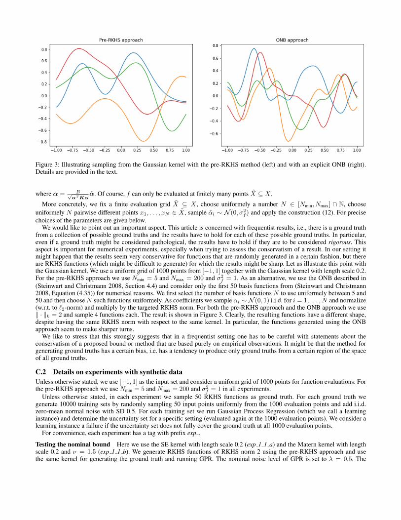
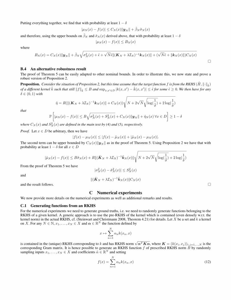
Figure 3: Illustrating sampling from the Gaussian kernel with the pre-RKHS method (left) and with an explicit ONB (right).Details are provided in the text.

where α = B√αTKα

α. Of course, f can only be evaluated at finitely many points X ⊆ X .

More concretely, we fix a finite evaluation grid X ⊆ X , choose uniformely a number N ∈ [Nmin, Nmax] ∩ N, chooseuniformely N pairwise different points x1, . . . , xN ∈ X , sample αi ∼ N (0, σ2

f ) and apply the construction (12). For precisechoices of the parameters are given below.

We would like to point out an important aspect. This article is concerned with frequentist results, i.e., there is a ground truthfrom a collection of possible ground truths and the results have to hold for each of these possible ground truths. In particular,even if a ground truth might be considered pathological, the results have to hold if they are to be considered rigorous. Thisaspect is important for numerical experiments, especially when trying to assess the conservatism of a result. In our setting itmight happen that the results seem very conservative for functions that are randomly generated in a certain fashion, but thereare RKHS functions (which might be difficult to generate) for which the results might be sharp. Let us illustrate this point withthe Gaussian kernel. We use a uniform grid of 1000 points from [−1, 1] together with the Gaussian kernel with length scale 0.2.For the pre-RKHS approach we use Nmin = 5 and Nmax = 200 and σ2

f = 1. As an alternative, we use the ONB described in(Steinwart and Christmann 2008, Section 4.4) and consider only the first 50 basis functions from (Steinwart and Christmann2008, Equation (4.35)) for numerical reasons. We first select the number of basis functions N to use uniformely between 5 and50 and then chooseN such functions uniformely. As coefficients we sample αi ∼ N (0, 1) i.i.d. for i = 1, . . . , N and normalize(w.r.t. to `2-norm) and multiply by the targeted RKHS norm. For both the pre-RKHS approach and the ONB approach we use‖ · ‖k = 2 and sample 4 functions each. The result is shown in Figure 3. Clearly, the resulting functions have a different shape,despite having the same RKHS norm with respect to the same kernel. In particular, the functions generated using the ONBapproach seem to make sharper turns.

We like to stress that this strongly suggests that in a frequentist setting one has to be careful with statements about theconservatism of a proposed bound or method that are based purely on empirical observations. It might be that the method forgenerating ground truths has a certain bias, i.e. has a tendency to produce only ground truths from a certain region of the spaceof all ground truths.

C.2 Details on experiments with synthetic dataUnless otherwise stated, we use [−1, 1] as the input set and consider a uniform grid of 1000 points for function evaluations. Forthe pre-RKHS approach we use Nmin = 5 and Nmax = 200 and σ2

f = 1 in all experiments.Unless otherwise stated, in each experiment we sample 50 RKHS functions as ground truth. For each ground truth we

generate 10000 training sets by randomly sampling 50 input points uniformly from the 1000 evaluation points and add i.i.d.zero-mean normal noise with SD 0.5. For each training set we run Gaussian Process Regression (which we call a learninginstance) and determine the uncertainty set for a specific setting (evaluated again at the 1000 evaluation points). We consider alearning instance a failure if the uncertainty set does not fully cover the ground truth at all 1000 evaluation points.

For convenience, each experiment has a tag with prefix exp .

Testing the nominal bound Here we use the SE kernel with length scale 0.2 (exp 1 1 a) and the Matern kernel with lengthscale 0.2 and ν = 1.5 (exp 1 1 b). We generate RKHS functions of RKHS norm 2 using the pre-RKHS approach and usethe same kernel for generating the ground truth and running GPR. The nominal noise level of GPR is set to λ = 0.5. The

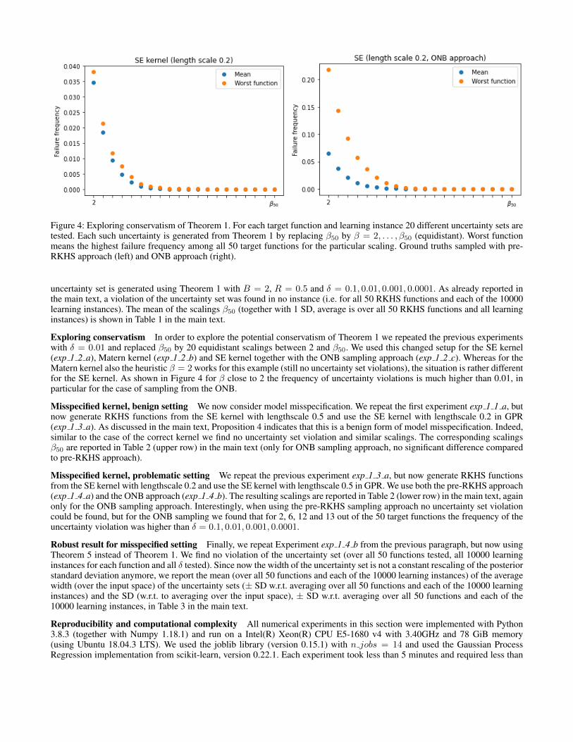
Figure 4: Exploring conservatism of Theorem 1. For each target function and learning instance 20 different uncertainty sets aretested. Each such uncertainty is generated from Theorem 1 by replacing β50 by β = 2, . . . , β50 (equidistant). Worst functionmeans the highest failure frequency among all 50 target functions for the particular scaling. Ground truths sampled with pre-RKHS approach (left) and ONB approach (right).

uncertainty set is generated using Theorem 1 with B = 2, R = 0.5 and δ = 0.1, 0.01, 0.001, 0.0001. As already reported inthe main text, a violation of the uncertainty set was found in no instance (i.e. for all 50 RKHS functions and each of the 10000learning instances). The mean of the scalings β50 (together with 1 SD, average is over all 50 RKHS functions and all learninginstances) is shown in Table 1 in the main text.

Exploring conservatism In order to explore the potential conservatism of Theorem 1 we repeated the previous experimentswith δ = 0.01 and replaced β50 by 20 equidistant scalings between 2 and β50. We used this changed setup for the SE kernel(exp 1 2 a), Matern kernel (exp 1 2 b) and SE kernel together with the ONB sampling approach (exp 1 2 c). Whereas for theMatern kernel also the heuristic β = 2 works for this example (still no uncertainty set violations), the situation is rather differentfor the SE kernel. As shown in Figure 4 for β close to 2 the frequency of uncertainty violations is much higher than 0.01, inparticular for the case of sampling from the ONB.

Misspecified kernel, benign setting We now consider model misspecification. We repeat the first experiment exp 1 1 a, butnow generate RKHS functions from the SE kernel with lengthscale 0.5 and use the SE kernel with lengthscale 0.2 in GPR(exp 1 3 a). As discussed in the main text, Proposition 4 indicates that this is a benign form of model misspecification. Indeed,similar to the case of the correct kernel we find no uncertainty set violation and similar scalings. The corresponding scalingsβ50 are reported in Table 2 (upper row) in the main text (only for ONB sampling approach, no significant difference comparedto pre-RKHS approach).

Misspecified kernel, problematic setting We repeat the previous experiment exp 1 3 a, but now generate RKHS functionsfrom the SE kernel with lengthscale 0.2 and use the SE kernel with lengthscale 0.5 in GPR. We use both the pre-RKHS approach(exp 1 4 a) and the ONB approach (exp 1 4 b). The resulting scalings are reported in Table 2 (lower row) in the main text, againonly for the ONB sampling approach. Interestingly, when using the pre-RKHS sampling approach no uncertainty set violationcould be found, but for the ONB sampling we found that for 2, 6, 12 and 13 out of the 50 target functions the frequency of theuncertainty violation was higher than δ = 0.1, 0.01, 0.001, 0.0001.

Robust result for misspecified setting Finally, we repeat Experiment exp 1 4 b from the previous paragraph, but now usingTheorem 5 instead of Theorem 1. We find no violation of the uncertainty set (over all 50 functions tested, all 10000 learninginstances for each function and all δ tested). Since now the width of the uncertainty set is not a constant rescaling of the posteriorstandard deviation anymore, we report the mean (over all 50 functions and each of the 10000 learning instances) of the averagewidth (over the input space) of the uncertainty sets (± SD w.r.t. averaging over all 50 functions and each of the 10000 learninginstances) and the SD (w.r.t. to averaging over the input space), ± SD w.r.t. averaging over all 50 functions and each of the10000 learning instances, in Table 3 in the main text.

Reproducibility and computational complexity All numerical experiments in this section were implemented with Python3.8.3 (together with Numpy 1.18.1) and run on a Intel(R) Xeon(R) CPU E5-1680 v4 with 3.40GHz and 78 GiB memory(using Ubuntu 18.04.3 LTS). We used the joblib library (version 0.15.1) with n jobs = 14 and used the Gaussian ProcessRegression implementation from scikit-learn, version 0.22.1. Each experiment took less than 5 minutes and required less than

1.5GiB memory (monitored using htop). Note that all experiments can easily be up and down scaled, depending on the availablehardware.

C.3 Control exampleWe now provide more details on the control example from Section 4.2.

Background For convenience we now provide a cursory overview of background material from control theory. We can onlyprovide a sketch and refer to standard textbooks for more details, e.g. (Astrom and Murray 2010) for a general introduction tocontrol and (Rawlings, Mayne, and Diehl 2017) for a comprehensive introduction to MPC.

A common goal in control is feedback stabilization under state and input constraints. Consider a discrete-time dynamicalsystem (or control system) described by

x+ = f(x, u)

with state space X , input space U and transition function f : X × U → X . For simplicity assume that X = Rn, U = Rmand that f(0, 0) = 0, i.e., (0, 0) is an equilibrium. Furthermore, consider state constraints X ⊆ X and input constraints U ⊆ U .Feedback stabilization amounts now to finding a map µ : X → U such that x∗ = 0 is an asymptotically stable equilibrium forthe resulting closed loop system described by

x+ = f(x, µ(x)),

and all resulting state-input trajectories are contained in the constraint set X×U. Note that this requires restriction of the set ofpossible initial values.

In many applications not only stability, but also a form of optimality is required from the control system. For example, assumethat being in state x and applying input u incurs a cost of `(x, u). If the control system is run for a long time, then we wouldlike a feedback µ that not only stabilizes the system, but also incurs a small infinite horizon cost

∞∑n=0

`(x(n), µ(x(n))),

where x(n) is the resulting state trajectory.One common methodology for dealing with state constraints and optimal control tasks is MPC. If the system is in state x,

MPC solves a finite horizon open loop problem, i.e. it determines a sequence u(0), . . . , u(N − 1) of admissible input valuesthat minimize some cost criterion. Only the first input u(0) is applied to the system and this process is repeated at the next timeinstance. There is a comprehensive theory available on how to design the open loop optimal control problem solved in eachinstance, in order to achieve desired closed loop properties. For details we refer to Chapters 1 and 2 in (Rawlings, Mayne, andDiehl 2017).

In many applications a control system has to deal with disturbances. Frequently the disturbances can be modelled in anadditive manner, i.e. we have a control system of the form

x+ = f(x, u) + w,

wherew ∈W ⊆ Rn is an external disturbance. The feedback stabilization problem under constraints can now be adapted to thissetting, resulting in robust feedback stabilization under constraints. The goal is now to find a feedback that ensures constraintsatisfaction and stabilizes the origin in a relaxed sense (which depends on the size of the disturbance set W). Furthermore, evenin this more challenging situation one might have to deal with additional cost criterions.

MPC can be adapted to the setting with disturbances. The key idea of most approaches is to solve a constrained open loopoptimal control problem where the constraints are tightened. The intuition is that even the worst case disturbance cannot throwthe system out of the allowed state-input set. It is clear that this requires sufficiently small bounds on the size of the disturbances.For more details we refer to Chapter 3 in (Rawlings, Mayne, and Diehl 2017).

Details on the example The control example in the main text is from Section 6 in (Soloperto et al. 2018). It consists of thefollowing system [

x+1x+2

]=

[0.995 0.095−0.095 0.900

] [x1x2

]+

[0.0480.95

]u+

[0

−r(x2)

](13)

modelling a mass-spring-damper system with some nonlinearity r (this could be interpreted as a friction term). As describedin the main text, we replaced the Stribeck friction curve used by (Soloperto et al. 2018) with a synthetic nonlinearity generatedfrom a known RKHS. Furthermore, the nonlinearity is assumed to be unknown and has to be learned from data. The controlgoal is the stabilization of the origin subject to the state and control constraints X = [−10, 10]× [−10, 10] and U = [−3, 3], aswell as minimizing a quadratic cost `(x, u) = 10‖x‖+ ‖u‖.

The RMPC approach from(Soloperto et al. 2018) performs this task by interpreting (13) as a linear system with disturbance,given by the nonlinearity r, whose graph is a-priori known to lie in the set W0 = [−10, 10] × [−7, 7]. The RMPC algorithmrequires as an input disturbance sets W(x) such that (0 −r(x2))

> ∈ W(x) for all x ∈ X, which are in turn used to generate

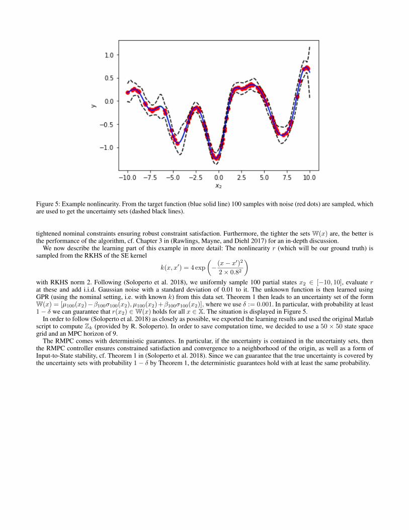
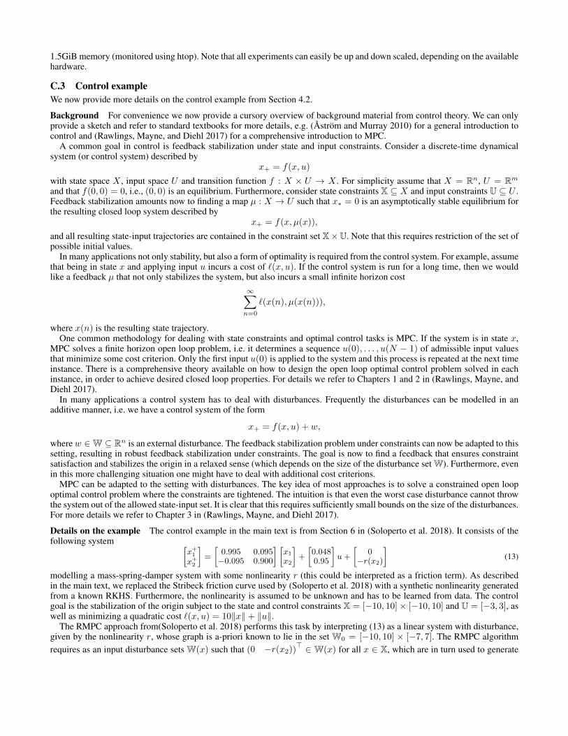
Figure 5: Example nonlinearity. From the target function (blue solid line) 100 samples with noise (red dots) are sampled, whichare used to get the uncertainty sets (dashed black lines).

tightened nominal constraints ensuring robust constraint satisfaction. Furthermore, the tighter the sets W(x) are, the better isthe performance of the algorithm, cf. Chapter 3 in (Rawlings, Mayne, and Diehl 2017) for an in-depth discussion.

We now describe the learning part of this example in more detail: The nonlinearity r (which will be our ground truth) issampled from the RKHS of the SE kernel

k(x, x′) = 4 exp

(− (x− x′)2

2× 0.82

)with RKHS norm 2. Following (Soloperto et al. 2018), we uniformly sample 100 partial states x2 ∈ [−10, 10], evaluate rat these and add i.i.d. Gaussian noise with a standard deviation of 0.01 to it. The unknown function is then learned usingGPR (using the nominal setting, i.e. with known k) from this data set. Theorem 1 then leads to an uncertainty set of the formW(x) = [µ100(x2)−β100σ100(x2), µ100(x2)+β100σ100(x2)], where we use δ := 0.001. In particular, with probability at least1− δ we can guarantee that r(x2) ∈W(x) holds for all x ∈ X. The situation is displayed in Figure 5.

In order to follow (Soloperto et al. 2018) as closely as possible, we exported the learning results and used the original Matlabscript to compute Zk (provided by R. Soloperto). In order to save computation time, we decided to use a 50 × 50 state spacegrid and an MPC horizon of 9.

The RMPC comes with deterministic guarantees. In particular, if the uncertainty is contained in the uncertainty sets, thenthe RMPC controller ensures constrained satisfaction and convergence to a neighborhood of the origin, as well as a form ofInput-to-State stability, cf. Theorem 1 in (Soloperto et al. 2018). Since we can guarantee that the true uncertainty is covered bythe uncertainty sets with probability 1− δ by Theorem 1, the deterministic guarantees hold with at least the same probability.