JOURNAL OF FUNCTIONAL ANALYSIS 80, 16-32 (1988)

Gaussian Upper Bounds for the Heat Kernels of Some Second-Order Operators on Riemannian Manifolds

E. B. DAVIES

Department of Mathematics, King’s College, Strand, London WC2R ZLS, England

Communicated by L. Gross

Received May 21, 1987

We describe a method of obtaining Gaussian upper bounds on heat kernels which unities and improves recent results for hypoelliptic operators in divergence form, and for Laplace-Beltrami operators on complete Riemannian manifolds. 0 1988 Academic Press, Inc.

1. INTRODUCTION

In the last few years Gaussian upper and lower bounds for the heat ker- nels of second-order operators H on Riemannian manifolds M have been subjected to intense study. For the case of uniformly elliptic operators in divergence form on RN see [8, 121. The most sophisticated results at present available compare the heat kernel K(t, x, y) of eeH’ with a function of the type

c~(x, t) fj(y, t) eCp2’a’ (1.1)

on (0, co) x A4 x M, where p(x, y) is the distance between x and y for a certain metric and 4(x, t) is defined in terms of the volumes of certain “balls” with centre x and radius t”*.

The fist results of the type which we mention are for a hypoelliptic operator H in the divergence form

where Xi are smooth vector fields on A4 satisfying Hormander’s conditions [13, 1618, 21, 231. In this case there is a rather singular metric pH associated with the operator, and 4(x, t)* is the Riemannian volume of the “ball”

B(x, P)= {yEM:p,(x,y)<t”*}. 16

0022-1236/88 $3.00 Copyright 0 1988 by Academic Press, Inc. All rights of reproduction in any form reserved.

GAUSSIAN BOUNDS FOR HEAT KERNELS 17

It was proved in [ 16181 that K(t, x, y) is bounded above and below by ( 1. I ) with different constants a and c for the upper and lower bounds. Our contribution to this problem is to prove that one can take a as close to 4 as one wishes, at least for the upper bound.

The second problem concerns similar estimates for the heat kernel of the Laplace-Beltrami operator on a complete Riemannian manifold, where 4(x, t)* is now the volume of the Riemannian ball with centre x and radius t”‘. Li and Yau [20] have proved that K(t, x, y) has upper and lower bounds of the form (1.1) with a arbitrarily close to 4 in both cases, provided the Ricci curvature is non-negative. Other papers on this problem obtain weaker bounds or involve further geometrical conditions which force 4(x, t) to have some special form [3, 5, 11, 193. We provide a sim- plification of a part of the proof of the upper bound in [20], and also prove new upper bounds on K(t, x, y) when one only assumes that the Ricci curvature is bounded below by some negative constant. In this case the bottom of the spectrum of H need not be zero and enters the calculations in a crucial manner.

Our method of approach in both problems is to obtain “off-diagonal” upper bounds on K( t, x, v) from easier “diagonal” bounds on K( t, x, x), by using logarithmic Sobolev inequalities as in [S-lo, 151. The method is general but necessitates additional refinements compared with earlier ver- sions, and is presented in Section 2. In Section 3 we apply it to hypoelliptic operators in divergence form, and in Sections 4 and 5 we apply it to Laplace-Beltrami operators.

2. THE ABSTRACT THEORY

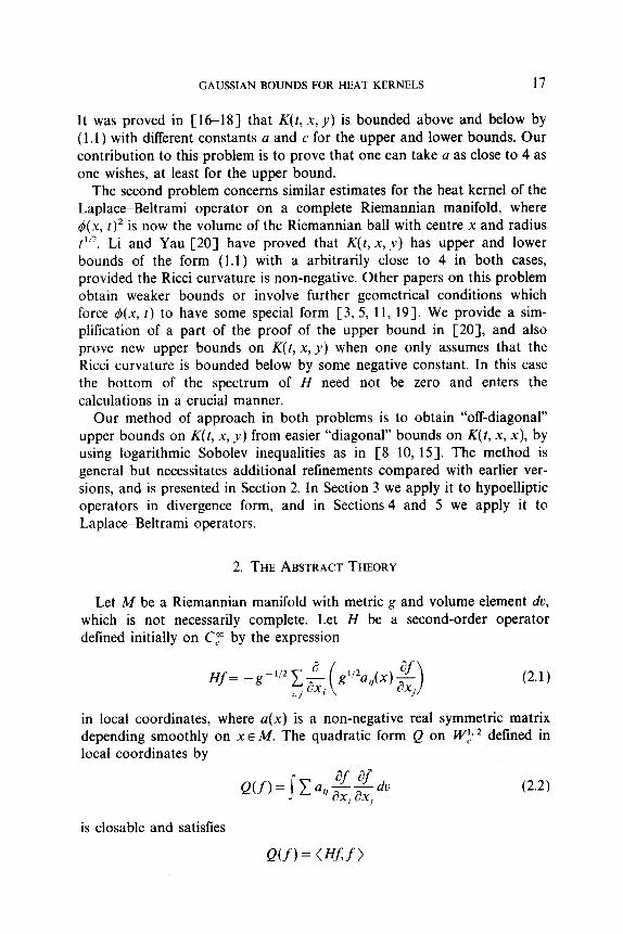
Let M be a Riemannian manifold with metric g and volume element du, which is not necessarily complete. Let H be a second-order operator defined initially on CT by the expression

g’/2a,j(x) E J

(2.1)

in local coordinates, where a(x) is a non-negative real symmetric matrix depending smoothly on x E M. The quadratic form Q on WJ* 2 defined in local coordinates by

(2.2)

is closable and satisfies

Q(f,=<Hf,f>

18 E. B. DAVIES

for all f E CF. We take H to be the self-adjoint operator associated with the form closure of Q [6,14], so that H> 0 and CF s Dam(H). If M is com- plete and H is the Laplace-Beltrami operator on A4 then H is already essentially self-adjoint on Cp, but we make neither of these assumptions. It is a standard consequence of the theory of Dirichlet forms [14,22] that epH’ is positivity preserving for all t > 0 and satisfies

for all 1 <p < cc and f~ LP(M). Finally, let p be the metric on A4 defined by

P(X, Y) = sup Hx) - KY): I(/ E A>, (2.3)

where A is the class of C” hounded functions rl/ on A4 such that

(2.4)

If H is the LaplaceBeltrami operator then it may be seen that p coincides with the Riemannian metric.

Our goal is to obtain upper bounds on the heat kernel K(t, x, y) of e-“’ in terms of p and a function 4(x, t) > 0 defined for x E M and 0 < t < S, where 0 < S < co. We assume that 4 is a positive continuous function with locally bounded first derivatives which satisfies

(2.5)

(2.6)

for constants A > 0 and F> 0 and all 0 < t < S, both differential inequalities being interpreted in the weak sense. We also assume throughout this section that e-“’ has a heat kernel for all t > 0 such that

0 < K(t, x, x) < cdw, t12 (2.7)

for xEMand O<t<S. Given any 0 < T< S we define the unitary operator U, from

L2(A4,qi(x, T)’ du) to L2(M, du) by

U,f(x) = 4(x, T)f(x)

and transfer the problem to this weighted L2 space. Putting

&4x)=4(x, T) Wx)

19 GAUSSIAN BOUNDS FOR HEAT KERNELS

we define H, on L2( M, du T) by

H,= U*,(TH+ F) UT

so that HT is associated with the form closure of

QAf)=TQ(4Tf)+FIlfll:

initially defined on W:, 2 c_ L*(M, du,); note that Wf, * is invariant under multiplication by q5; r . A standard calculation using (2.6) shows that

where pr is a non-negative measure on M. In the application of this theory in Section 4 it will turn out that pr may be singular with respect to V, because of cut locus behaviour. Since QT is a Dirichlet form we see [14,22] that e-Hrr is positivity preserving with

lie-“Yfll,~ Ilfll,

for all 1 <p< co and fe Lp(M, do.).

LEMMA 1. If 0 -C t d 1 then the heat kernel K, of eCHrr satisfies

O<K,(t,x,y)<c,t-A’2.

Proof: A direct calculation shows that

K( Tt, x, Y) Wf, xy yke-” 4(x, T) +(y, T)’ (2.9)

Since K is the kernel of a positive operator we see from (2.7) that

0 < K(s, x, y) < K(s, x, x)“* K(s, y, Y)“~

G GM% s) 4(Y, s).

Therefore

(2.8)

20 E. B. DAVIES

and the proof is completed by the bound

F4$b(X, Tc) d f$(x, T) < t-A’4q4(X, Tr)

provable for 0 < t < 1 using (2.5).

(2.10)

LEMMA 2. If 2<p<m andO<&<l,

s f”logfdu,~&(H,f,fP-‘)+2B(&)P-’ Ilf II;+ Ilf Il;log Ilf lip (2.11)

for all 0 < f E CF , where

/3(E) = c, - $4 log E.

Proof The inequality (2.8) is equivalent to the logarithmic Sobolev inequality

5 f*logfd+<GMf >+L%)llf II:+ Ilf Il:log Ilfll2

by standard arguments [2, lo]. It is also equivalent [2, 121 to the Nash inequality

Ilf II:+“‘“G{<&f,f >+ Ilf II3 Ilf IIY

and if A > 2 to the Sobolev inequality [25]

II f II L,(A - 2) ~~2wMf >+ Ilf II37

but we prefer to work with log Sobolev inequalities because of their ability to handle more singular problems [7, lo]. If we replace f by fp’* and use the inequality [25; 24, p. 1831

(&(fp/*),fp/*) <& (HTf,f”-‘>

then (2.11) follows. In fact in our context (2.12) may be proved by integration by parts as in [ 10, 151, since H, is a local operator.

LEMMA 3. Let 5 = ea*, where aE[W, and let $:M+ R be C” and bounded with

GAUSSIAN BOUNDSFORHEAT KERNELS 21

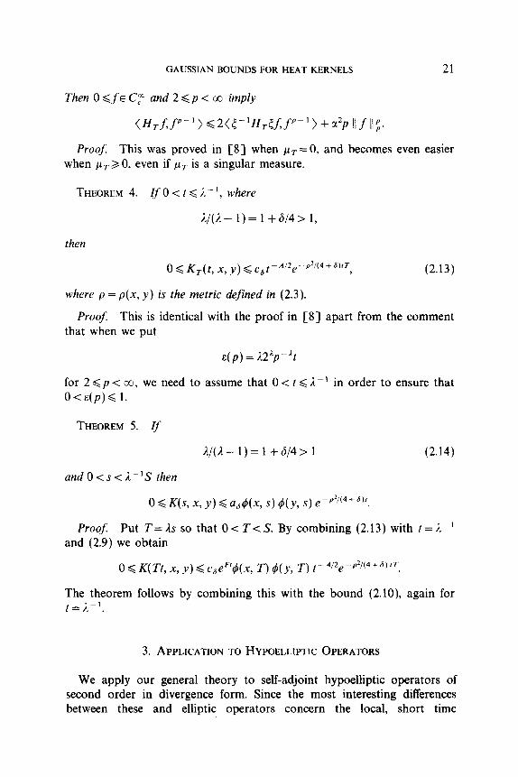
Then 0 d f E CpO and 2 < p < co imply

(HTf,f~-‘I)~22(5-1Hrrf,fP-1)+~2P Ilf 11;.

Proof. This was proved in [8] when pT = 0, and becomes even easier when p T > 0, even if p T is a singular measure.

THEOREM 4. If 0 < t < ,I - ‘, where

A/(ls- l)= 1 +q4> 1,

then

0 d K,(t, x, y) < ~~t~~~*e--~~‘(~+~)‘~, (2.13)

where p = p(x, y) is the metric defined in (2.3).

Proof. This is identical with the proof in [8] apart from the comment that when we put

E(P) = 12ip--“t

for 2 <p -=z co, we need to assume that 0 < t d ;1- ’ in order to ensure that O<&(P)< 1.

THEOREM 5. If

A/( A- 1) = 1 + 6/4 > 1 (2.14)

andO<s<k’S then

Proof. Put T= As so that 0 < T< S. By combining (2.13) with t = A ~ I and (2.9) we obtain

0 d K(Tt, x, y) < c6eFtcj(x, T) 4(y, T) t-Ai*e-p2’(4+6)‘T.

The theorem follows by combining this with the bound (2.10), again for t=r’.

3. APPLICATION TO HYPOELLIPTIC OPERATORS

We apply our general theory to self-adjoint hypoelliptic operators of second order in divergence form. Since the most interesting differences between these and elliptic operators concern the local, short time

22 E. B. DAVIES

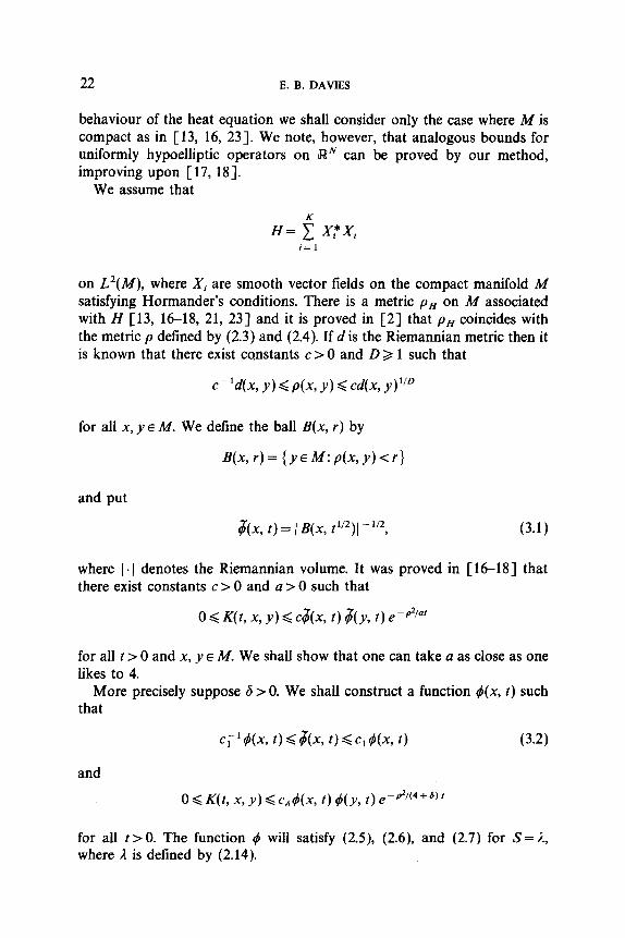
behaviour of the heat equation we shall consider only the case where M is compact as in [ 13, 16, 231. We note, however, that analogous bounds for uniformly hypoelliptic operators on IV’ can be proved by our method, improving upon [17,18].

We assume that

H= 2 X,?Xi i=l

on L’(M), where Xi are smooth vector fields on the compact manifold M satisfying Hormander’s conditions. There is a metric P,, on A4 associated with H [13, 16-18, 21, 231 and it is proved in [2] that pH coincides with the metric p defined by (2.3) and (2.4). If d is the Riemannian metric then it is known that there exist constants c > 0 and D 2 1 such that

c-ld(x, y) < p(x, y) < cd@, yPD

for all x, y E A4. We define the ball B(x, r) by

q&r)= {Y~~:ph9<r)

and put

&x, t) = 1 B(x, tq -1’2, (3.1)

where 1.1 denotes the Riemannian volume. It was proved in [ 16-183 that there exist constants c > 0 and a > 0 such that

OiK(t,x,y)<c&x, t)&y, t)e-P2’a’

for all t > 0 and x, y E M. We shall show that one can take a as close as one likes to 4.

More precisely suppose 6 > 0. We shall construct a function &x, t) such that

c;‘4(x, t) G &x, t) G c, 4(x, t) (3.2)

and

O<K(t,x,y)<c,#(x, t)d(y, t)e-p2i(4+6)t

for all t > 0. The function 4 will satisfy (2.5), (2.6), and (2.7) for S= A, where 1 is defined by (2.14).

GAUSSIAN BOUNDS FOR HEAT KERNELS 23

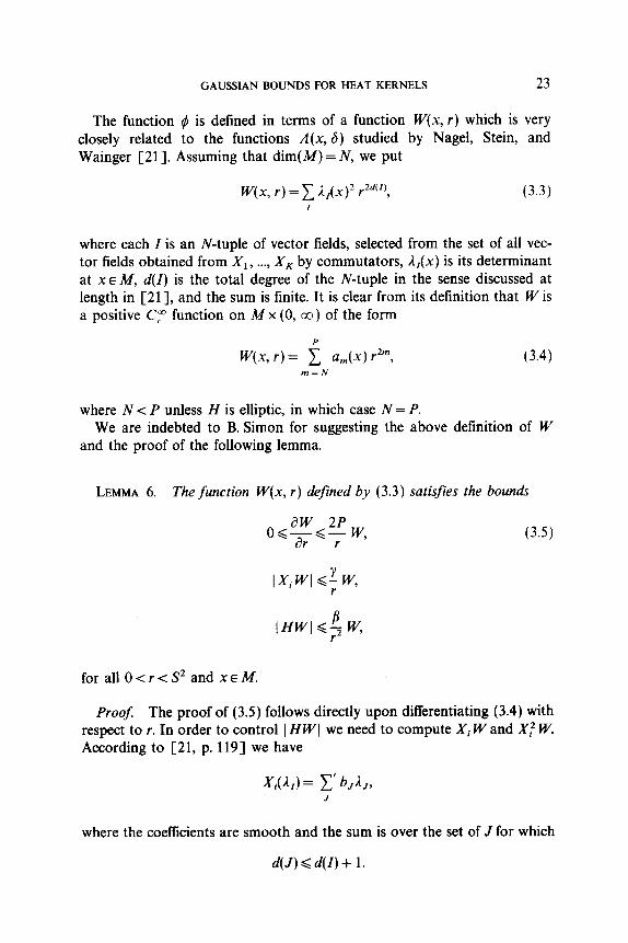
The function q5 is defined in terms of a function W(x, r) which is very closely related to the functions /i(x, 6) studied by Nagel, Stein, and Wainger [21]. Assuming that dim(M)=N, we put

W(x, r) = 1 /l,(x)2 r2d(‘),

where each Z is an N-tuple of vector fields, selected from the set of all vec- tor fields obtained from Xi, . . . . X, by commutators, n,(x) is its determinant at XE M, d(Z) is the total degree of the N-tuple in the sense discussed at length in [21], and the sum is finite. It is clear from its definition that W is a positive Cy function on M x (0, cc) of the form

P

W(x, r)= 1 a,(x) rZm, (3.4) m=N

where N < P unless H is elliptic, in which case N = P. We are indebted to B. Simon for suggesting the above definition of W

and the proof of the following lemma.

LEMMA 6. The function W(x, r) defined by (3.3) satisfies the bounds

O<>&C~ w, (3.5) r

for all Ocr<S’and XEM.

Proof The proof of (3.5) follows directly upon differentiating (3.4) with respect to r. In order to control 1 HWI we need to compute Xi W and X,? W. According to [21, p. 1191 we have

xi(n,) = 1’ bJ&, J

where the coefficients are smooth and the sum is over the set of J for which

d(J) < d(Z) + 1.

24 E. B. DAVIES

Therefore 0 -=z Y -=z S* implies

c,, Jjl,AJY2d(‘)

d(J) < d(l) + 1

Similarly

H(W) = 1’ b,, K&&r2d(r), J, K

where bJ. K is smooth and the sum is restricted to those J, K for which

d(J) + d(K) < 2d(Z) + 2.

Therefore 0 < r < S2 implies

I H( W)l <; 1 )1,1 /,I,/ rd(J)+d(K) J, K

B < - w.

r2

LEMMA 7. Zf we define 4(x, t) for x E M and 0 < t < S by

(6(x, t) = W(x, t”*)y4

then there exist constants A and F depending upon 6 > 0 such that (2.5) and (2.6) hold for all 0 < t < S.

Proof: This is a direct computation using the bounds of Lemma 6.

LEMMA 8. There exists a constant c> 0 for which (3.2) holds for all xEMandO<t<l.

Proof: If we put

A(x, r) = C I AI(x)1 rd(‘)

then the Schwarz inequality implies that

GAUSSIANBOUNDSFOR HEATKERNELS 25

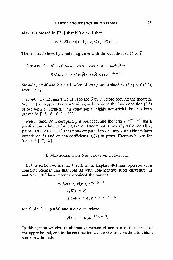
Also it is proved in [21] that if 0 <r < 1 then

cj- I I B(x, r)l < A(x, r) < c2 I B(x, r)l.

The lemma follows by combining these with the definition (3.1) of 6.

THEOREM 9. Jf 6 > 0 there exists a constant cs such that

O<K(t,x,y)<c,$(x, t)&y, t)epf”(4+6”

for all x, y E A4 and 0 < t < 1, where 6 and p are defined by (3.1) and (2.3), respectively.

Proof. By Lemma 8 we can replace 6 by 4 before proving the theorem. We can then apply Theorem 5 with S = J provided the final condition (2.7) of Section 2 is verified. This condition is highly non-trivial, but has been proved in [13, 1618, 21, 231.

Note. Since M is compact, p is bounded, and the term e -p2’(4+6)’ has a positive lower bound for 1 < t -C co, Theorem 9 is actually valid for all x, y E M and 0 < t < co. If M is non-compact then one needs suitable.uniform bounds on M and on the coefficients a&x) to prove Theorem 9 even for O<t<l [17,18].

4. MANIFOLDS WITH NON-NEGATIVE CURVATURE

In this section we assume that H is the Laplace-Beltrami operator on a complete Riemannian manifold M with non-negative Ricci curvature. Li and Yau [20] have recently obtained the bounds

c;‘qS(x, t)&y, t)e-p2”4m &jr

< wt, & y)

Qc,#(x, t)qS(y, t)eppZ!‘4+6)r

for all 6>0, x, REM, and O<t<oo, where

r#(x, t) = ) B(x, t1’2)i p”2.

In this section we give an alternative version of one part of their proof of the upper bound, and in the next section we use the same method to obtain some new bounds.

26 E. B. DAVIES

We start by quoting the Harnack inequality of [20, Theorem 2.21. This states that if u is a positive solution of the heat equation then

O<u(x, t)<u(y, t+s) 7 ( ) t + f Ni2 ep2/4s

for all s > 0, t > 0, x, y E M, where p = p(x, y) is the distance between x and y in M and dim M = N. Our first result is a simple special case of [20, Theorem 3.11.

LEMMA 10. There exists a constant c depending only upon N such that

0 < K(t, x, x) < c 1 B(x, F2)l -l

for aNxEMandO<t<co.

Proof The Harnack inequality (4.1) implies that

K(t,x,x)dK(t+s,y,x) y- ( ) t + s N12 erzj4s

provided t > 0, s > 0, and y lies in the ball B with centre x and radius r > 0. Therefore

since e - H’ is a contradiction semigroup on L’(M). The lemma now follows upon putting s = t = r2.

We shall once again apply the general theory of Section 2 for a suitable function 4(x, t), which is of the same order of magnitude as (B(x, t’j2)( -l12. We start by defining the function V(x, r) for XEM and s> 0 by

where f is a C” decreasing function on [O, co) with f (s) = 1 if 0 ,< s < 1 and f(s)=0 if 2Gs<co.

LEMMA 11. There exists a constant cl > 0 such that

I H-T r)lG Vx, r) <cl I+, r)l

forallx~Mandr~0.

GAUSSIAN BOUNDS FOR HEAT KERNELS 27

Proof. It is immediate from the definition that

l&x, r)l 6 V(x, r) 6 I B(x, 2r)l

and we may now use [4, Proposition 4.11.

LEMMA 12. We have the bounds

for all xfM and r>O.

Proof. We have

where f’ < 0. Therefore

0 <tJ< c;r-’ ) B(x, 2r)J

6 c, c;r-’ 1 B(x, r)l

< c2rp1V(x, r).

Second,

SO

l’W~r~l~(f’(~)ldy

< c;r-’ I B(x, 2r)l

< c3re1V(x, r).

Finally,

28 E. B. DAVIES

Now a theorem of Calabi [I; 3, p. 1851 states that

APG(N--l)lp,

where the derivatives are weak. Therefore

(4.3)

and

LEMMA 13. If

4(x, t) = V(x, c2)p2 (4.4)

then there exist positive constants A and F such that

forallxEMandO<t<oo.

Proof: This is proved by a direct computation using the bounds of Lemma 12.

THEOREM 14. If M is complete with non-negative Ricci curvature then the heat kernel satisfies

O<K(t,x,y)<c, IB(x, t”2)I-‘/2 IB(y, t1~2))-‘~2e~p2~(4+S)t

for all6>0, x,y~M, andO<t<oo.

Proof: We apply the theory of Section 2 with S = 00 and 4 defined by (4.4). It follows from Lemma 11 that 4(x, t) is comparable with 1 B(x, t”2)1 -‘j2 and from Lemmas 10 and 13 that the conditions (2.5), (2.6), and (2.7) of Section 2 are satisfied. The theorem is now a special case of Theorem 5.

GAUSSIAN BOUNDS FOR HEAT KERNELS 29

Note. This theorem is due to Li and Yau [20, Theorem 3.11, who also obtain a lower bound of the same order [20, Theorem 4.11 by a separate calculation. Their method is entirely different from ours, and they comment that it does not yield very good bounds when extended to manifolds with Ricci curvature bounded below by a negative constant.

5. MANIFOLDS WITH NEGATIVE CURVATURE

In this section we assume that M is a complete Riemannian manifold of dimension N such that

Ric(x)> -(N- 1) f12

for all x E M. We let E 2 0 denote the bottom of the spectrum of the operator H = -A, and note that although E is a global invariant of the manifold, it is not easy to express it in geometrical terms. If j? = 0 then E = 0, but in the general case E enters into the heat kernel estimates in a crucial manner.

Our first lemma differs from the estimates of Li and Yau [20] in that it involves E.

LEMMA 15. If E > 0 then there exists c, such that

0 < K(t, x, x) d c, 1 B(x, t”‘)J -’ e’” E)’ (5-l)

forallxEMandt>O.

Proof If u is a positive solution of the heat equation on M then putting q = 0, y =O, 8 = 0, a = 4 in [20, Theorem 2.2(ii) J we obtain the Harnack inequality

3NJ4 exp( cs + dp’/s)

for all s > 0, t > 0, x, y E M, where p is the distance between x and y and c, d are constants. Applying this to the heat kernel we see that if p(x, y) < r and p(x, z) < r then

K(t,x,x)<K(t+s,x,y)

exp( 2cs + 2dr2/s).

30 E. B. DAVIES

If B is the ball with centre x and radius r then integrating y and z over B yields

I BJ’K(t, x, x)< (e-ncr+2s)Xs, xs)

Putting r = t “* and s = 6t for some 6 > 0 we obtain

K(t, x, x) < 1 BI -’ e-E”1+2g) (1 + 26)3N’4 exp(2c& + 2d/6)

from which the lemma follows by putting

E-E=2c6-E(l +26).

We note that the first term on the right-hand side of (5.1) is dominant for small l> 0 while the second term is dominant for large t. We therefore estimate K(t, x, y) separately for 0 < t < 1 and for 1 < t < co.

IfJ>OwedefineA=S>l by

A/(4-1)=1+6/4

as in Theorem 5, and observe that Lemma 15 implies that

0 < K(t, x, x) <as 1 B(x, +‘*)I -I

for all xEMand O<t<S.

THEOREM 16. There exists a constant cb depending upon 6 such that

0~ K(t, x, y) < c6 ) B(x, t”*)( -‘I* 1 B(y, t’/*)l -I’* e-p2’(4+6)f

forallx,yEMandO<t<l.

Proof: If we define V(x, r) for 0 < r < S* by (4.2) then Lemma 11 is still valid. If we define 4(x, t) for 0 < t < S by (4.4) then Lemma 13 is still valid, although Calabi’s inequality (4.3) is replaced by the weaker version [ 1; 3, p. 185-J

Ap < (N - 1) coth(/-Q)

G CIP

for 0 < p < S*. The remainder of the proof follows that of Theorem 14.

GAUSSIAN BOUNDS FOR HEAT KERNELS 31

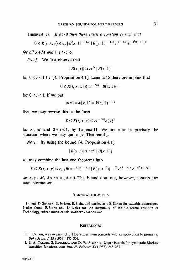
THEOREM 17. If 6>0 then there exists a constant c6 such that

O<K(t,x,y)<c, \B(x, 1)1-“* IB(y, 1)1-“2e(s-E)te--p2’(4+6)’

forallxEMandl<t<co.

Proof. We first observe that

I B(x, r)l2 crN I B(x, 1 )I

for 0 < r < 1 by [4, Proposition 4.11. Lemma 15 therefore implies that

O<K(t,x,x)<ct-N’* IE(x, l)l-’

for O<t<l. If we put

cT(x)=qqx, l)= V(x, 1))“2

then we may rewrite this in the form

0 < K(t, x, x) < et -N’*cT(X)*

for XE M and 0 < t i 1, by Lemma 11. We are now in precisely the situation where we may quote [9, Theorem 43.

Note. By using the bound [4, Proposition 4.11

lB(x,r)l<cea’lB(x, 111

we may combine the last two theorems into

O<K(t,X,y)<Cc, lE(x, t”*)lel’* (B(y, t”2)~-“2e(d--E)te-p2(4+d)’

for X, y E M, 0 < t < co,6 > 0. This bound does not, however, contain any new information.

ACKNOWLEDGMENTS

I thank D. Stroock, D. Jerison, E. Stein, and particularly B. Simon for valuable discussions. I also thank E. Stone and D. Wales for the hospitality of the California Institute of Technology, where much of this work was carried out.

REFERENCES

1. E. CALABI, An extension of E.‘HopTs maximum principle with an application to geometry, Duke Math. J. 25 (1965), 285-303.

2. E. A. CARLEN, S. KUSUOKA, AND D. W. STROOCK, Upper bounds for symmetric Markov transition functions, Ann. Inst. H. Poincarb 23 (1987) 245-287.

580/80!1-3

32 E. B. DAVIES

3. I. CHAVEL, “Eigenvalues in Riemannian Geometry,” Academic Press, Orlando, FL. 1984. 4. J. CHEEGER, M. GROMOV, AND M. TAYLOR, Finite propagation speed, kernel estimates for

functions of the Laplace operator, and the geometry of complete Riemannian manifolds, J. Differential Geom. 17 (1982), 15-53.

5. J. CHFEGER AND S. T. YAU, A lower bound for the heat kernel, Comm. Pure Appl. Math. 34 (1981), 465-480.

6. E. B. DAVIES, “One-Parameter Semigroups,” Academic Press, Orlando, FL, 1980. 7. E. B. DAVIES, Heat kernel bounds for second order elliptic operators on Riemannian

manifolds, Amer. J. Math. 109 (1987), 545-570. 8. E. B. DAVIES, Explicit constants for Gaussian upper bounds on heat kernels, Amer.

J. Math. 109 (1987), 319-334. 9. E. B. DAVIES AND N. MANDOUVALOS, Heat kernel bounds on manifolds with cusps,

J. Funct. Anal. 75 (1987), 311-322. 10. E. B. DAVIES AND B. SIMON, Ultracontractivity and the heat kernel for Schrodinger

operators and Dirichlet Laplacians, J. Funct. Anal. 59 (1984), 335-395. 11. A. DEBIARD, B. GAVEAU, AND E. MAZET, Theoremes de comparaisons en geometric

Riemannienne, Publ. Res. Inst. Math. Sci. 12 (1976), 391-425. 12. E. B. FABJZS AND D. W. STRDOCK, A new proof of Moser’s parabolic Harnack inequality

using the old ideas of Nash, Arch. Rational Mech. Anal. % (1986), 327-338. 13. C. FEFFERMAN AND S. SANCHEZ-CALLE, Fundamental solutions for second order subellip-

tic operators, Ann. of Math. 124 (1986), 247-272. 14. M. FUKUSHIMA, “Dirichlet Forms and Markov Processes,” North-Holland, Amsterdam,

1980. 15. L. GROss., Logarithmic Sobolev inequalities, Amer. J. Math. 97 (1976), 1061-1083. 16. D. S. JERI~ON AND A. SANCHEZ-CALLE, Estimates for the heat kernel for a sum of squares

of vector fields, Indiana Univ. J. Math. 35 (1986), 835-854. 17. S. KUSUOKA AND D. STROOCK, Applications of Malliabin calculus, Part 3, preprint, 1986. 18. S. KUSUOKA AND D. STROOCK, Long time estimates for the heat kernel associated with a

uniformly subelliptic second order operator, Ann. Math. 127 (1988), 165-189. 19. P. LI, Large time asymptotics of the heat equation on complete manifolds with

non-negative Ricci curvature, Ann. of Math. 124 (1986), l-21. 20. P. Lr AND S. T. YAU, On the parabolic kernel of the Schrodinger operator, Acta Math.

156 (1986), 153-201. 21. A. NAGEL, E. M. STEIN, AND S. WAINGER, Balls and metrics delined by vector fields. I.

Basic properties, Acta Math. 155 (1985), 103-147. 22. M. REED AND B. SIMON, “Methods of Modern Mathematical Physics,” Vol. 4, Academic

Press, Orlando, FL, 1978. 23. A. SANCHEZ-CALLE, Fundamental solutions and geometry of the sum of squares of vector

fields, Invent. Math. 78 (1984), 143-160. 24. D. STROOCK, “An Introduction to the Theory of Large Deviations,” Springer-Verlag,

New York/Berlin, 1984. 25. N. VAROFYXJLOS, Hardy-Littlewood theory for semigroups, J. Funct. Anal. 63 (1985),

24Ck260.