comparison and anti-concentration bounds …vchern/papers/anticoncentrationvectors-v10.pdf ·...

COMPARISON AND ANTI-CONCENTRATION BOUNDS

FOR MAXIMA OF GAUSSIAN RANDOM VECTORS

VICTOR CHERNOZHUKOV, DENIS CHETVERIKOV, AND KENGO KATO

Abstract. Slepian and Sudakov-Fernique type inequalities, which com-pare expectations of maxima of Gaussian random vectors under certainrestrictions on the covariance matrices, play an important role in proba-bility theory, especially in empirical process and extreme value theories.Here we give explicit comparisons of expectations of smooth functionsand distribution functions of maxima of Gaussian random vectors with-out any restriction on the covariance matrices. We also establish an anti-concentration inequality for the maximum of a Gaussian random vector,which derives a useful upper bound on the Levy concentration functionfor the Gaussian maximum. The bound is dimension-free and applies tovectors with arbitrary covariance matrices. This anti-concentration in-equality plays a crucial role in establishing bounds on the Kolmogorovdistance between maxima of Gaussian random vectors. These resultshave immediate applications in mathematical statistics. As an exampleof application, we establish a conditional multiplier central limit theoremfor maxima of sums of independent random vectors where the dimensionof the vectors is possibly much larger than the sample size.

1. Introduction

We derive a bound on the difference in expectations of smooth functionsof maxima of finite dimensional Gaussian random vectors. We also derive abound on the Kolmogorov distance between distributions of these maxima.The key property of these bounds is that they depend on the dimension p ofGaussian random vectors only through log p, and on the max norm of the dif-ference between the covariance matrices of the vectors. These results extendand complement the work of [7] that derived an explicit Sudakov-Ferniquetype bound on the difference of expectations of maxima of Gaussian randomvectors. See also [1], Chapter 2. As an application, we establish a condi-tional multiplier central limit theorem for maxima of sums of independentrandom vectors where the dimension of the vectors is possibly much largerthan the sample size. In all these results, we allow for arbitrary covariancestructures between the coordinates in random vectors, which is plausible

Date: First version: January 21, 2013. This version: April 13, 2014.2000 Mathematics Subject Classification. 60G15, 60E15, 62E20.Key words and phrases. Slepian inequality, anti-concentration, Levy concentration

function, maximum of Gaussian random vector, conditional multiplier central limittheorem.

1

2 CHERNOZHUKOV, CHETVERIKOV, AND KATO

especially in applications to high-dimensional statistics. We stress that thederivation of bounds on the Kolmogorov distance is by no means trivialand relies on a new anti-concentration inequality for maxima of Gaussianrandom vectors, which is another main result of this paper (see Comment4 for what anti-concentration inequalities here precisely refer to and howthey differ from the concentration inequalities). These anti-concentrationbounds are non-trivial in the following sense: (i) they apply to every di-mension p and they are dimension-free in the sense that the bounds dependon the dimension p only through the expectation of the maximum of theGaussian random vector, thereby admitting direct extensions to the infinitedimensional case, namely, separable Gaussian processes (see [10] for this ex-tension and applications to empirical processes). This dimension-free natureis parallel to the Gaussian concentration inequality, which states that thesupremum concentrates around the expected supremum. (ii) They allow forarbitrary covariance structures between the coordinates in Gaussian randomvectors, and (iii) they are sharp in the sense that there is an example forwhich the bound is tight up to a dimension independent constant. We notethat these anti-concentration bounds are sharper than those that result fromapplication of the universal reverse isoperimetric inequality of [2] (see also[3], p.386-367).

Comparison inequalities for Gaussian random vectors play an importantrole in probability theory, especially in empirical process and extreme valuetheories. We refer the reader to [24], [14], [12], [16], [17], [18], [7], and [30] forstandard references on this topic. The anti-concentration phenomenon hasattracted considerable interest in the context of random matrix theory andthe Littlewood-Offord problem in number theory. See, for example, [22], [23],and [29] who remarked that “concentration is better understood than anti-concentration”. Those papers were concerned with the anti-concentration inthe Euclidean norm for sums of independent random vectors, and the topicand the proof technique here are substantially different from theirs.

Either of the comparison or anti-concentration bounds derived in the pa-per have many immediate statistical applications, especially in the contextof high-dimensional statistical inference, where the dimension p of vectors ofinterest is much larger than the sample size (see [5] for a textbook treatmentof the recent developments of high-dimensional statistics). In particular,the results established here are helpful in deriving an invariance principlefor sums of high-dimensional random vectors, and also in establishing thevalidity of the multiplier bootstrap for inference in practice. We refer thereader to our companion paper [9], where the results established here areapplied in several important statistical problems, particularly the analysisof Dantzig selector of [6] in the non-Gaussian setting.

The proof strategy for our anti-concentration inequalities is to directlybound the density function of the maximum of a Gaussian random vec-tor. The paper by [20] is concerned with bounding such a density (see [20],Proposition 3.12) but under positive covariances restriction. This is related

COMPARISON AND ANTI-CONCENTRATION 3

to but different from our anti-concentration bounds. The crucial assump-tion in their Proposition 3.12 is positivity of all the covariances betweenthe coordinates in the Gaussian random vector, which does not hold in ourtargeted applications in high-dimensional statistics, for example, analysis ofDanzig selector. Moreover, their upper bound on the density depends onthe inverse of the lower bound on the covariances – and hence, for example,if there are two independent coordinates in the Gaussian random vector,then the upper bound becomes infinite. Our anti-concentration bounds donot require such positivity (or other) assumptions on covariances and henceare not implied by the results of [20]. Another method for deriving reverseisoperimetric inequalities is to use geometric results of [19], as shown by [13],which leads to dimension-dependent anti-concentration inequalities, whichare essentially different from ours. Moreover, our density-bounding prooftechnique is substantially different from that of [20] based on Malliavin cal-culus or [19] based on geometric arguments.

The rest of the paper is organized as follows. In Section 2, we presentcomparison bounds for Gaussian random vectors and its application, namelythe conditional multiplier central limit theorem. In Section 3, we presentanti-concentration bounds for maxima of Gaussian random vectors. In Sec-tions 4 and 5, we give proofs of the theorems in Sections 2 and 3. TheAppendix contains a proof of a technical lemma.

Notation. Denote by (Ω,F ,P) the underlying probability space. Fora, b ∈ R, we write a+ = max0, a and a ∨ b = maxa, b. Let 1(·) denotethe indicator function. The transpose of a vector z is denoted by zT . For afunction g : R→ R, we use the notation ‖g‖∞ = supz∈R |g(z)|. Let φ(·) andΦ(·) denote the density and distribution functions of the standard Gaussian

distribution, respectively: φ(x) = (1/√

2π)e−x2/2 and Φ(x) =

∫ x−∞ φ(t)dt.

2. Comparison Bounds and Multiplier Bootstrap

2.1. Comparison bounds. Let X = (X1, . . . , Xp)T and Y = (Y1, . . . , Yp)

T

be centered Gaussian random vectors in Rp with covariance matrices ΣX =(σXjk)1≤j,k≤p and ΣY = (σYjk)1≤j,k≤p, respectively. The purpose of this sec-tion is to give error bounds on the difference of the expectations of smoothfunctions and the distribution functions of

max1≤j≤p

Xj and max1≤j≤p

Yj

in terms of p,

∆ := max1≤j,k≤p

|σXjk − σYjk|, and ap := E[ max1≤j≤p

(Yj/σYjj)].

The problem of comparing distributions of maxima is of intrinsic diffi-culty since the maximum function z = (z1, . . . , zp)

T 7→ max1≤j≤p zj is non-differentiable. To circumvent the problem, we use a smooth approximation


of the maximum function. For z = (z1, . . . , zp)T ∈ Rp, consider the function:

Fβ(z) := β−1 log

p∑j=1

exp(βzj)

,

which approximates the maximum function, where β > 0 is the smoothingparameter that controls the level of approximation (we call this function the“smooth max function”). Indeed, an elementary calculation shows that forevery z ∈ Rp,

0 ≤ Fβ(z)− max1≤j≤p

zj ≤ β−1 log p. (1)

This smooth max function arises in the definition of “free energy” in spinglasses. See, for example, [27] and [21]. Here is the first theorem of thissection.

Theorem 1 (Comparison bounds for smooth functions). For every g ∈C2(R) with ‖g′‖∞ ∨ ‖g′′‖∞ <∞ and every β > 0,

|E[g(Fβ(X))− g(Fβ(Y ))]| ≤ (‖g′′‖∞/2 + β‖g′‖∞)∆,

and hence

|E[g( max1≤j≤p

Xj)− g( max1≤j≤p

Yj)]| ≤ (‖g′′‖∞/2 + β‖g′‖∞)∆ + 2β−1‖g′‖∞ log p.

Proof. See Section 4.

Comment 1. Minimizing the second bound with respect to β > 0, we have

|E[g( max1≤j≤p

Xj)− g( max1≤j≤p

Yj)]| ≤ ‖g′′‖∞∆/2 + 2‖g′‖∞√

2∆ log p.

This result extends the work of [7], which derived the following Sudakov-Fernique type bound on the expectation of the difference between two Gauss-ian maxima:

|E[ max1≤j≤p

Xj − max1≤j≤p

Yj ]| ≤ 2√

2∆ log p.

Theorem 1 is not applicable to functions of the form g(z) = 1(z ≤ x) andhence does not directly lead to a bound on the Kolmogorov distance betweenmax1≤j≤pXj and max1≤j≤p Yj (recall that the Kolmogorov distance between(the distributions) of two real valued random variables ξ and η is defined bysupx∈R |P(ξ ≤ x)− P(η ≤ x)|). Nevertheless, we have the following boundson the Kolmogorov distance. Recall ap = E[max1≤j≤p(Yj/σ

Yjj)].

Theorem 2 (Comparison of distributions). Suppose that p ≥ 2 and σYjj > 0for all 1 ≤ j ≤ p. Then

supx∈R|P( max

1≤j≤pXj ≤ x)− P( max

1≤j≤pYj ≤ x)|

≤ C∆1/3

(1 ∨ a2p ∨ log(1/∆)1/3

log1/3 p, (2)


where C > 0 depends only on min1≤j≤p σYjj and max1≤j≤p σ

Yjj (the right

side is understood to be 0 when ∆ = 0). Moreover, in the worst case,ap ≤

√2 log p, so that

supx∈R|P( max

1≤j≤pXj ≤ x)− P( max

1≤j≤pYj ≤ x)| ≤ C ′∆1/31 ∨ log(p/∆)2/3,

where as before C ′ > 0 depends only on min1≤j≤p σYjj and max1≤j≤p σ

Yjj.

Proof. See Section 4.

The first bound (2) is generally sharper than the latter. To see this,consider the simple case where ap = O(1) as p → ∞, which would happen,for example, when Y1, . . . , Yp come from discretization of a single continuousGaussian process. Then the right side on (2) is o(1) if ∆(log p) log log p =o(1), while the second bound requires ∆(log p)2 = o(1).

Comment 2 (On the proof strategy). Bounding the Kolmogorov distancebetween max1≤j≤pXj and max1≤j≤p Yj is not immediate from Theorem 1and this step relies on the anti-concentration inequality for the maximum of aGaussian random vector, which we will study in Section 3. More formally, bysmoothing the indicator and maximum functions, we obtain from Theorem1 a bound of the following form:

infβ,δ>0

L( max1≤j≤p

Yj , β−1 log p+ δ) + C(δ−2 + βδ−1)∆,

where L(max1≤j≤p Yj , ε) is the Levy concentration function for max1≤j≤p Yj(see Definition 1 in Section 3 for the formal definition), and β, δ > 0 aresmoothing parameters (see equations (10) and (11) in the proof of Theorem2 given in Section 4 for the derivation of the above bound). The bound(2) then follows from bounding the Levy concentration function by usingthe anti-concentration inequality derived in Section 3, and optimizing thebound with respect to β, δ.

The proof of Theorem 2 is substantially different from the (“textbook”)proof of classical Slepian’s inequality. The simplest form of Slepian’s in-equality states that

P( max1≤j≤p

Xj ≤ x) ≤ P( max1≤j≤p

Yj ≤ x), ∀x ∈ R,

whenever σXjj = σYjj and σXjk ≤ σYjk for all 1 ≤ j, k ≤ p. This inequality isimmediately deduced from the following expression:

P( max1≤j≤p

Xj ≤ x)− P( max1≤j≤p

Yj ≤ x)

=∑

1≤j<k≤p(σXjk − σYjk)

∫ 1

0

∫ x

−∞· · ·∫ x

−∞

∂2ft(z)

∂zj∂zkdz

dt, (3)

where σXjj = σYjj , 1 ≤ ∀j ≤ p, is assumed. Here ft denotes the density

function of N(0, tΣX + (1 − t)ΣY ). See [14], p.82, for this expression. Theexpression (3) is of importance and indeed a source of many interesting


probabilistic results (see, for example, [18] and [30] for recent related works).It is not clear (or at least non-trivial), however, whether a bound similar innature to Theorem 2 can be deduced from the expression (3) when thereis no restriction on the covariance matrices except for the condition thatσXjj = σYjj , 1 ≤ ∀j ≤ p, and here we take the different route.

The key features of Theorem 2 are: (i) the bound on the Kolmogorovdistance between the maxima of Gaussian random vectors in Rp dependson the dimension p only through log p and the maximum difference of thecovariance matrices ∆, and (ii) it allows for arbitrary covariance matrices forX and Y (except for the nondegeneracy condition that σYjj > 0, 1 ≤ ∀j ≤ p).These features have an important implication to statistical applications, asdiscussed below.

2.2. Conditional multiplier central limit theorem. Consider the fol-lowing problem. Suppose that n independent centered random vectors inRp of observations Z1, . . . , Zn are given. Here Z1, . . . , Zn are generally non-Gaussian, and the dimension p is allowed to increase with n (that is, thecase where p = pn → ∞ as n → ∞ is allowed). We suppress the possibledependence of p on n for the notational convenience. Suppose that each Zihas a finite covariance matrix E[ZiZ

Ti ]. Consider the following normalized

sum:

Sn := (Sn,1, . . . , Sn,p)T =

1√n

n∑i=1

Zi.

The problem here is to approximate the distribution of max1≤j≤p Sn,j .Statistics of this form arise frequently in modern statistical applications.

The exact distribution of max1≤j≤p Sn,j is generally unknown. An intuitiveidea to approximate the distribution of max1≤j≤p Sn,j is to use the Gaussianapproximation. Let V1, . . . , Vn be independent Gaussian random vectors inRp such that Vi ∼ N(0,E[ZiZ

Ti ]), and define

Tn := (Tn,1, . . . , Tn,p) :=1√n

n∑i=1

Vi ∼ N(0, n−1∑n

i=1E[ZiZTi ]).

It is expected that the distribution of max1≤j≤p Tn,j is close to that ofmax1≤j≤p Sn,j in the following sense:

supx∈R|P( max

1≤j≤pSn,j ≤ x)− P( max

1≤j≤pTn,j ≤ x)| → 0, n→∞. (4)

When p is fixed, (4) will follow from the classical Lindeberg-Feller centrallimit theorem, subject to the Lindeberg conditions. The recent paper by [9]established conditions under which this Gaussian approximation (4) holdseven when p is comparable or much larger than n. For example, [9] provedthat if c1 ≤ n−1

∑ni=1 E[Z2

ij ] ≤ C1 and E[exp(|Zij |/C1)] ≤ 2 for all 1 ≤ i ≤ nand 1 ≤ j ≤ p for some 0 < c1 < C1, then (4) holds as long as log p = o(n1/7).

The Gaussian approximation (4) is in itself an important step, but in thegeneral case where the covariance matrix n−1

∑ni=1 E[ZiZ

Ti ] is unknown, it


is not directly applicable for purposes of statistical inference. In such cases,the following multiplier bootstrap procedure will be useful. Let η1, . . . , ηnbe independent standard Gaussian random variables independent of Zn1 :=Z1, . . . , Zn. Consider the following randomized sum:

Sηn := (Sηn,1, . . . , Sηn,p)

T :=1√n

n∑i=1

ηiZi.

Since conditional on Zn1 ,

Sηn ∼ N(0, n−1∑n

i=1ZiZTi ),

it is natural to expect that the conditional distribution of max1≤j≤p Sηn,j is

“close” to the distribution of max1≤j≤p Tn,j and hence that of max1≤j≤p Sn,j .Note here that the conditional distribution of Sηn is completely known, whichmakes this distribution useful for purposes of statistical inference. The fol-lowing proposition makes this intuition rigorous.

Proposition 1 (Conditional multiplier central limit theorem). Work withthe setup as described above. Suppose that p ≥ 2 and there are some con-stants 0 < c1 < C1 such that c1 ≤ n−1

∑ni=1 E[Z2

ij ] ≤ C1 for all 1 ≤ j ≤ p.

Moreover, suppose that ∆ := max1≤j,k≤p |n−1∑n

i=1(ZijZik − E[ZijZik])|obeys the following conditions: as n→∞,

∆(E[ max1≤j≤p

Tn,j ])2 log p = oP(1), ∆(log p)(1 ∨ log log p) = oP(1). (5)

Then we have

supx∈R|P( max

1≤j≤pSηn,j ≤ x | Z

n1 )− P( max

1≤j≤pTn,j ≤ x)| P→ 0, as n→∞. (6)

Here recall that p is allowed to increase with n.

Proof. Follows immediately from Theorem 2.

We call this result a “conditional multiplier central limit theorem,” wherethe terminology follows that in empirical process theory. See [28], Chapter2.9. The notable features of this proposition, which inherit from the featuresof Theorem 2 discussed above, are: (i) (6) can hold even when p is muchlarger than n, and (ii) it allows for arbitrary covariance matrices for Zi(except for the mild scaling condition that c1 ≤ n−1

∑ni=1 E[Z2

ij ] ≤ C1). Thesecond point is clearly desirable in statistical applications as the informationon the true covariance structure is generally (but not always) unavailable.

For the first point, we have the following estimate on E[∆].

Lemma 1. Let p ≥ 2. There exists a universal constant C > 0 such that

E[∆] ≤ C

[max1≤j≤p

(n−1∑n

i=1E[Z4ij ])

1/2

√log p

n+ (E[ max

1≤i≤nmax1≤j≤p

Z4ij ])

1/2 log p

n

].

Proof. See the Appendix.


Hence with help of Lemma 2.2.2 in [28], we can find various primitiveconditions under which (5) holds.

Example 1. Consider the following examples. Here for the sake of sim-plicity, we use the worst case bound E[max1≤j≤p Tn,j ] ≤

√2C1 log p, so that

conditions (5) reduce to ∆ = oP((log p)−2).Case (a): Suppose that E[exp(|Zij |/C1)] ≤ 2 for all 1 ≤ i ≤ n and

1 ≤ j ≤ p for some C1 > 0. In this case, it is not difficult to verify that

∆ = oP((log p)−2) as soon as log p = o(n1/5).Case (b): Another type of Zij which arises in regression applications

is of the form Zij = εixij where εi are stochastic with E[εi] = 0 andmax1≤i≤n E[|εi|4q] = O(1) for some q ≥ 1, and xij are non-stochastic (typ-ically, εi are “errors” and xij are “regressors”). Suppose that xij are nor-malized in such a way that n−1

∑ni=1 x

2ij = 1, and there are bounds Bn ≥ 1

such that max1≤i≤n max1≤j≤p |xij | ≤ Bn, where we allow Bn → ∞. In this

case, ∆ = oP((log p)−2) as soon as

maxB2n(log p)5, B4q/(2q−1)

n (log p)6q/(2q−1) = o(n),

since max1≤j≤p(n−1∑n

i=1 E[(εixij)4]) ≤ B2

n max1≤i≤n E[ε4i ] = O(B2n) and

E[max1≤i≤n max1≤j≤p(εixij)4] ≤ B4

nE[max1≤i≤n ε4i ] = O(n1/qB4

n).Importantly, in these examples, for (6) to hold, p can increase exponen-

tially in some fractional power of n.

3. Anti-concentration Bounds

The following theorem provides bounds on the Levy concentration func-tion of the maximum of a Gaussian random vector in Rp, where the termi-nology is borrowed from [23].

Definition 1 ([23], Definition 3.1). The Levy concentration function of areal valued random variable ξ is defined for ε > 0 as

L(ξ, ε) = supx∈R

P(|ξ − x| ≤ ε).

Theorem 3 (Anti-concentration). Let (X1, . . . , Xp)T be a centered Gauss-

ian random vector in Rp with σ2j := E[X2j ] > 0 for all 1 ≤ j ≤ p. Moreover,

let σ := min1≤j≤p σj , σ := max1≤j≤p σj, and ap := E[max1≤j≤p(Xj/σj)].(i) If the variances are all equal, namely σ = σ = σ, then for every ε > 0,

L( max1≤j≤p

Xj , ε) ≤ 4ε(ap + 1)/σ.

(ii) If the variances are not equal, namely σ < σ, then for every ε > 0,

L( max1≤j≤p

Xj , ε) ≤ Cεap +√

1 ∨ log(σ/ε),

where C > 0 depends only on σ and σ.


Since Xj/σj ∼ N(0, 1), by a standard calculation, we have ap ≤√

2 log pin the worst case (see, for example, [27], Proposition 1.1.3), so that thefollowing simpler corollary follows immediately from Theorem 3.

Corollary 1. Let (X1, . . . , Xp)T be a centered Gaussian random vector in

Rp with σ2j := E[X2j ] > 0 for all 1 ≤ j ≤ p. Let σ := min1≤j≤p σj and

σ := max1≤j≤p σj. Then for every ε > 0,

L( max1≤j≤p

Xj , ε) ≤ Cε√

1 ∨ log(p/ε),

where C > 0 depends only on σ and σ. When σj are all equal, log(p/ε) onthe right side can be replaced by log p.

Comment 3 (Anti-concentration vs. small ball probabilities). The problemof bounding the Levy concentration function L(max1≤j≤pXj , ε) is qualita-tively different from the problem of bounding P(max1≤j≤p |Xj | ≤ x). For asurvey on the latter problem, called the “small ball problem”, we refer thereader to [17].

Comment 4 (Concentration vs. anti-concentration). Concentration in-equalities refer to inequalities bounding P(|ξ−x| > ε) for a random variableξ (typically x is the mean or median of ξ). See the monograph [15] fora study of the concentration of measure phenomenon. Anti-concentrationinequalities in turn refer to reverse inequalities, that is, inequalities bound-ing P(|ξ − x| ≤ ε). Theorem 3 provides anti-concentration inequalities formax1≤j≤pXj . [29] remarked that “concentration is better understood thananti-concentration”. In the present case, the Gaussian concentration in-equality (see [15], Theorem 7.1) states that

P(| max1≤j≤p

Xj − E[ max1≤j≤p

Xj ]| ≥ r) ≤ 2e−r2/(2σ2), r > 0,

where the mean can be replace by the median. This inequality is well knownand dates back to [4] and [26]. To the best of our knowledge, however, thereverse inequalities in Theorem 3 were not known and are new.

Comment 5 (Anti-concentration for maximum of moduli, max1≤j≤p |Xj |).Versions of Theorem 3 and Corollary 1 continue to hold for max1≤j≤p |Xj |.That is, for example, when σj are all equal (σj = σ), L(max1≤j≤p |Xj |, ε) ≤4(a′p + 1)/σ, where a′p := E[max1≤j≤p |Xj |/σ]. To see this, observe thatmax1≤j≤p |Xj | = max1≤j≤2pX

′j where X ′j = Xj for j = 1, . . . , p and X ′p+j =

−Xj for j = 1, . . . , p. Hence we may apply Theorem 3 to (X ′1, . . . , X′2p)

T toobtain the desired conclusion.

Comment 6 (A sketch of the proof of Theorem 3). For the reader’s con-venience, we provide a sketch of the proof of Theorem 3. We focus here onthe simple case where all the variances are equal to one (σ1 = · · · = σp = 1).Then the distribution of Z = max1≤j≤pXj is absolutely continuous andits density can be written as φ(z)G(z) where the map z 7→ G(z) is non-decreasing. Consequently, it is then not difficult to see that G(z) ≤ P(Z >


z)/1−Φ(z) ≤ 2(z∨1)e−(z−ap)2+/2/φ(z), where the second inequality follows

from Mill’s inequality combined with the Gaussian concentration inequality.

Hence the density of Z is bounded by 2(z∨1)e−(z−ap)2+/2, which immediately

leads to the bound L(max1≤j≤pXj , ε) ≤ 4(ap + 1)ε.

In a trivial example where p = 1, it is immediate to see that P(|X1−x| ≤ε) ≤ ε

√2/(πσ21). A non-trivial case is the situation where p → ∞. In

such a case, it is typically not known whether max1≤j≤pXj has a limitingdistribution as p → ∞, even after normalization (recall that except forσ > 0, we allow for general covariance structures between X1, . . . , Xp), andtherefore it is not trivial at all whether, for every sequence ε = εp → 0 (orat some rate), L(max1≤j≤pXj , ε) → 0 or how fast ε = εp → 0 should be toguarantee that L(max1≤j≤pXj , ε) → 0. Theorem 3 answers this questionwith explicit, non-asymptotic bounds.

Importantly, the bounds in Theorem 3 are dimension-free in the sensethat, similar to the Gaussian concentration inequality, they depend on thedimension p only through ap – the expectation of the maximum of the (nor-malized) Gaussian random vector. Hence Theorem 3 admits direct exten-sions to the infinite dimensional case, namely separable Gaussian processes,as long as the corresponding expectation is finite. See our companion paper[10] for formal treatments and applications of this extension.

The presence of ap on the bounds is essential and can not be removedin general, as the following example suggests. This shows that there doesnot exist a substantially sharper estimate of the universal bound of theconcentration function than that given in Theorem 3. Potentially, therecould be refinements but they would have to rely on the particular (hencenon-universal) features of the covariance structure between X1, . . . , Xp.

Example 2 (Partial converse of Theorem 3). LetX1, . . . , Xp be independentstandard Gaussian random variables. By Theorem 1.5.3 of [14], as p→∞,

bp( max1≤j≤p

Xj − dp)d→ G(0, 1), (7)

where

bp :=√

2 log p, dp := bp −log(4π) + log log p

2bp,

and G(0, 1) denotes the standard Gumbel distribution, that is, the distri-

bution having the density g(x) = e−xe−e−x

for x ∈ R. In fact, we canshow that the density of bp(max1≤j≤pXj − dp) converges to that of G(0, 1)locally uniformly. To see this, we begin with noting that the density ofbp(max1≤j≤pXj − dp) is given by

gp(x) =p

bpφ(dp + b−1p x)[Φ(dp + b−1p x)]p−1.

Pick any x ∈ R. Since, by the weak convergence result (7),

[Φ(dp + b−1p x)]p = P(bp( max1≤j≤p

Xj − dp) ≤ x)→ e−e−x, p→∞,


we have [Φ(dp + b−1p x)]p−1 → e−e−x

. Hence it remains to show that

p

bpφ(dp + b−1p x)→ e−x.

Taking the logarithm of the left side yields

log p− log bp − log(√

2π)− (dp + b−1p x)2/2. (8)

Expanding (dp + b−1p x)2 gives that

d2p + 2dpb−1p x+ b−2p x2 = b2p − log log p− log(4π) + 2x+ o(1), p→∞,

by which we have (8) = −x + o(1). This shows that gp(x) → g(x) for allx ∈ R. Moreover, this convergence takes place locally uniformly in x, thatis, for every K > 0, gp(x)→ g(x) uniformly in x ∈ [−K,K].

On the other hand, the density of max1≤j≤pXj is given by fp(x) =pφ(x)[Φ(x)]p−1. By this form, for every K > 0, there exist a constantc > 0 and a positive integer p0 depending only on K such that for p ≥ p0,

infx∈[dp−Kb−1

p ,dp+Kb−1p ]b−1p fp(x) = inf

x∈[−K,K]gp(x) ≥ inf

x∈[−K,K]g(x) + o(1) ≥ c,

which shows that for p ≥ p0,

fp(x) ≥ cbp, ∀x ∈ [dp −Kb−1p , dp +Kb−1p ].

Therefore, we conclude that for p ≥ p0,

P(| max1≤j≤p

Xj − dp| ≤ ε) =

∫ dp+ε

dp−εfp(x)dx ≥ 2cεbp, ∀ε ∈ [0,Kb−1p ].

By the Gaussian maximal inequality and Lemma 2.3.15 of [11], we have√log p/12 ≤ E[ max

1≤j≤pXj ] ≤

√2 log p.

Hence, by the previous result, for every K ′ > 0, there exist a constant c′ > 0and and a positive integer p′0 depending only on K ′ such that for p ≥ p′0,ap ≥ 1 and

L( max1≤j≤p

Xj , ε) ≥ P(| max1≤j≤p

Xj − dp| ≤ ε) ≥ c′εap, ∀ε ∈ [0,K ′a−1p ].

4. Proofs for Section 2

4.1. Proof of Theorem 1. Here for a smooth function f : Rp → R, wewrite ∂jf(z) = ∂f(z)/∂zj for z = (z1, . . . , zp)

T . We shall use the followingversion of Stein’s identity.


Lemma 2 (Stein’s identity). Let W = (W1, . . . ,Wp)T be a centered Gauss-

ian random vector in Rp. Let f : Rp → R be a C1-function such thatE[|∂jf(W )|] <∞ for all 1 ≤ j ≤ p. Then for every 1 ≤ j ≤ p,

E[Wjf(W )] =

p∑k=1

E[WjWk]E[∂kf(W )].

Proof of Lemma 2. See Section A.6 of [27]; also [8] and [25].

We will use the following properties of the smooth max function.

Lemma 3. For every 1 ≤ j, k ≤ p,

∂jFβ(z) = πj(z), ∂j∂kFβ(z) = βwjk(z),

where

πj(z) := eβzj/∑p

m=1eβzm , wjk(z) := 1(j = k)πj(z)− πj(z)πk(z).

Moreover,

πj(z) ≥ 0,∑p

j=1πj(z) = 1,∑p

j,k=1|wjk(z)| ≤ 2.

Proof of Lemma 3. The first property was noted in [7]. The other propertiesfollow from a direct calculation.

Lemma 4. Let m := g Fβ with g ∈ C2(R). Then for every 1 ≤ j, k ≤ p,

∂j∂km(z) = (g′′ Fβ)(z)πj(z)πk(z) + β(g′ Fβ)(z)wjk(z),

where πj and wjk are defined in Lemma 3.

Proof of lemma 4. The proof follows from a direct calculation.

Proof of Theorem 1. Without loss of generality, we may assume that X andY are independent, so that E[XjYk] = 0 for all 1 ≤ j, k ≤ p. Consider thefollowing Slepian interpolation between X and Y :

Z(t) :=√tX +

√1− tY, t ∈ [0, 1].

Let m := g Fβ and Ψ(t) := E[m(Z(t))]. Then

|E[m(X)]− E[m(Y )]| = |Ψ(1)−Ψ(0)| =∣∣∣∣∫ 1

0Ψ′(t)dt

∣∣∣∣ .Here we have

Ψ′(t) =1

2

p∑j=1

E[∂jm(Z(t))(t−1/2Xj − (1− t)−1/2Yj)]

=1

2

p∑j=1

p∑k=1

(σXjk − σYjk)E[∂j∂km(Z(t))],


where the second equality follows from applying Lemma 2 toW = (t−1/2Xj−(1− t)−1/2Yj , Z(t)T )T and f(W ) = ∂jm(Z(t)). Hence∣∣∣∣∫ 1

0Ψ′(t)dt

∣∣∣∣ ≤ 1

2

p∑j,k=1

|σXjk − σYjk|∣∣∣∣∫ 1

0E[∂j∂km(Z(t))]dt

∣∣∣∣≤ 1

2max

1≤j,k≤p|σXjk − σYjk|

∫ 1

0

p∑j,k=1

|E[∂j∂km(Z(t))]| dt

=∆

2

∫ 1

0

p∑j,k=1

|E[∂j∂km(Z(t))]| dt.

By Lemmas 3 and 4,

p∑j,k=1

|∂j∂km(Z(t))| ≤ |(g′′ Fβ)(Z(t))|+ 2β|(g′ Fβ)(Z(t))|.

Therefore, we have

|E[g(Fβ(X))− g(Fβ(Y ))]|

≤ ∆×

1

2

∫ 1

0E[|(g′′ Fβ)(Z(t))|]dt+ β

∫ 1

0E[|(g′ Fβ)(Z(t))|]dt

≤ ∆(‖g′′‖∞/2 + β‖g′‖∞),

which leads to the first assertion. The second assertion follows from theinequality (1). This completes the proof.

4.2. Proof of Theorem 2. The final assertion follows from the inequalityap ≤

√2 log p (see, for example, [27], Proposition 1.1.3). Hence we prove

(2). We first note that we may assume that 0 < ∆ < 1 since otherwisethe proof is trivial (take C ≥ 2 in (2)). In what follows, let C > 0 be ageneric constant that depends only on min1≤j≤p σ

Yjj and max1≤j≤p σ

Yjj , and

its value may change from place to place. For β > 0, define ep,β := β−1 log p.Consider and fix a C2-function g0 : R → [0, 1] such that g0(t) = 1 for t ≤ 0and g0(t) = 0 for t ≥ 1. For example, we may take

g0(t) =

0, t ≥ 1,

30∫ 1t s

2(1− s)2ds, 0 < t < 1,

1, t ≤ 0.

For given x ∈ R, β > 0 and δ > 0, define gx,β,δ(t) = g0(δ−1(t − x − ep,β)).

For this function gx,β,δ, ‖g′x,β,δ‖∞ = δ−1‖g′0‖∞ and ‖g′′x,β,δ‖∞ = δ−2‖g′′0‖∞.Moreover,

1(t ≤ x+ ep,β) ≤ gx,β,δ(t) ≤ 1(t ≤ x+ ep,β + δ), ∀t ∈ R. (9)


For arbitrary x ∈ R, β > 0 and δ > 0, observe that

P( max1≤j≤p

Xj ≤ x) ≤ P(Fβ(X) ≤ x+ ep,β) ≤ E[gx,β,δ(Fβ(X))]

≤ E[gx,β,δ(Fβ(Y ))] + C(δ−2 + βδ−1)∆

≤ P(Fβ(Y ) ≤ x+ ep,β + δ) + C(δ−2 + βδ−1)∆

≤ P( max1≤j≤p

Yj ≤ x+ ep,β + δ) + C(δ−2 + βδ−1)∆, (10)

where the first inequality follows from the inequality (1), the second from theinequality (9), the third from Theorem 1, the fourth from the inequality (9),and the last from the inequality (1). We wish to compare P(max1≤j≤p Yj ≤x+ep,β+δ) with P(max1≤j≤p Yj ≤ x), and this is where the anti-concentrationinequality plays its role. By Theorem 3, we have

P( max1≤j≤p

Yj ≤ x+ ep,β + δ)− P( max1≤j≤p

Yj ≤ x)

= P(x < max1≤j≤p

Yj ≤ x+ ep,β + δ) ≤ L( max1≤j≤p

Yj , ep,β + δ) (11)

≤ C(ep,β + δ)√

1 ∨ a2p ∨ log1/(ep,β + δ) ≤ C(ep,β + δ)√

1 ∨ a2p ∨ log(1/δ).

Therefore,

P( max1≤j≤p

Xj ≤ x)− P( max1≤j≤p

Yj ≤ x)

≤ C

(δ−2 + βδ−1)∆ + (ep,β + δ)√

1 ∨ a2p ∨ log(1/δ). (12)

Take a = ap ∨ log1/2(1/∆), and choose β and δ in such a way that

β = δ−1 log p and δ = ∆1/3(1 ∨ a)−1/3(2 log p)1/3.

Recall that p ≥ 2 and 0 < ∆ < 1. Observe that (δ−2 +βδ−1)∆ ≤ C∆1/3(1∨a)2/3 log1/3 p, (ep,β + δ)(1 ∨ ap) ≤ C∆1/3(1 ∨ a)2/3 log1/3 p, and since δ ≥∆1/3(1∨a)−1/3, we have log(1/δ) ≤ (1/3) log((1∨a)/∆). Hence the right side

on (12) is bounded by C∆1/3(1∨a)2/3 log1/3 p+(1∨a)−1/3(log1/3 p) log1/2((1∨a)/∆). In addition, (1 ∨ a)−1 log1/2(1 ∨ a) is bounded by a universal con-stant, so that

right side of (12)

≤ C∆1/3(1 ∨ a)2/3 log1/3 p+ (1 ∨ a)−1/3(log1/3 p) log1/2(1/∆).

The second term inside the bracket is bounded by (log1/3 p) log1/3(1/∆) as

(1∨a)−1/3 ≤ (log(1/∆))−1/6, and first term is bound by (1∨ap)2/3 log1/3 p+

(log1/3 p) log1/3(1/∆). Adjusting the constant C, the right side on the above

displayed equation is bounded by C∆1/31 ∨ a2p ∨ log(1/∆)1/3 log1/3 p.


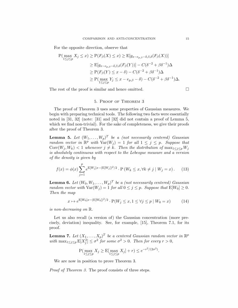
For the opposite direction, observe that

P( max1≤j≤p

Xj ≤ x) ≥ P(Fβ(X) ≤ x) ≥ E[gx−ep,β−δ,β,δ(Fβ(X))]

≥ E[gx−ep,β−δ,β,δ(Fβ(Y ))]− C(δ−2 + βδ−1)∆

≥ P(Fβ(Y ) ≤ x− δ)− C(δ−2 + βδ−1)∆

≥ P( max1≤j≤p

Yj ≤ x− ep,β − δ)− C(δ−2 + βδ−1)∆.

The rest of the proof is similar and hence omitted.

5. Proof of Theorem 3

The proof of Theorem 3 uses some properties of Gaussian measures. Webegin with preparing technical tools. The following two facts were essentiallynoted in [31, 32] (note: [31] and [32] did not contain a proof of Lemma 5,which we find non-trivial). For the sake of completeness, we give their proofsafter the proof of Theorem 3.

Lemma 5. Let (W1, . . . ,Wp)T be a (not necessarily centered) Gaussian

random vector in Rp with Var(Wj) = 1 for all 1 ≤ j ≤ p. Suppose thatCorr(Wj ,Wk) < 1 whenever j 6= k. Then the distribution of max1≤j≤pWj

is absolutely continuous with respect to the Lebesgue measure and a versionof the density is given by

f(x) = φ(x)

p∑j=1

eE[Wj ]x−(E[Wj ])2/2 · P (Wk ≤ x, ∀k 6= j |Wj = x) . (13)

Lemma 6. Let (W0,W1, . . . ,Wp)T be a (not necessarily centered) Gaussian

random vector with Var(Wj) = 1 for all 0 ≤ j ≤ p. Suppose that E[W0] ≥ 0.Then the map

x 7→ eE[W0]x−(E[W0])2/2 · P(Wj ≤ x, 1 ≤ ∀j ≤ p |W0 = x) (14)

is non-decreasing on R.

Let us also recall (a version of) the Gaussian concentration (more pre-cisely, deviation) inequality. See, for example, [15], Theorem 7.1, for itsproof.

Lemma 7. Let (X1, . . . , Xp)T be a centered Gaussian random vector in Rp

with max1≤j≤p E[X2j ] ≤ σ2 for some σ2 > 0. Then for every r > 0,

P( max1≤j≤p

Xj ≥ E[ max1≤j≤p

Xj ] + r) ≤ e−r2/(2σ2).

We are now in position to prove Theorem 3.

Proof of Theorem 3. The proof consists of three steps.


Step 1. This step reduces the analysis to the unit variance case. Pickany x ≥ 0. Let Wj := (Xj−x)/σj+x/σ. Then E[Wj ] ≥ 0 and Var(Wj) = 1.Define Z := max1≤j≤pWj . Then we have

P(| max1≤j≤p

Xj − x| ≤ ε) ≤ P

(∣∣∣∣max1≤j≤p

Xj − xσj

∣∣∣∣ ≤ ε

σ

)≤ sup

y∈RP

(∣∣∣∣max1≤j≤p

Xj − xσj

+x

σ− y∣∣∣∣ ≤ ε

σ

)= sup

y∈RP

(|Z − y| ≤ ε

σ

).

Step 2. This step bounds the density of Z. Without loss of generality,we may assume that Corr(Wj ,Wk) < 1 whenever j 6= k. Since the marginaldistribution of Wj is N(µj , 1) where µj := E[Wj ] = (x/σ − x/σj) ≥ 0, byLemma 5, Z has density of the form

fp(z) = φ(z)Gp(z), (15)

where the map z 7→ Gp(z) is non-decreasing by Lemma 6. Define z :=(1/σ − 1/σ)x, so that µj ≤ z for every 1 ≤ j ≤ p. Moreover, defineZ := max1≤j≤p(Wj − µj). Then∫ ∞

zφ(u)duGp(z) ≤

∫ ∞z

φ(u)Gp(u)du = P(Z > z)

≤ P(Z > z − z) ≤ exp

−

(z − z − E[Z])2+2

,

where the last inequality is due to the Gaussian concentration inequality(Lemma 7). Note that Wj − µj = Xj/σj , so that

E[Z] = E[ max1≤j≤p

(Xj/σj)] =: ap.

Therefore, for every z ∈ R,

Gp(z) ≤1

1− Φ(z)exp

−

(z − z − ap)2+2

. (16)

Mill’s inequality states that for z > 0,

z ≤ φ(z)

1− Φ(z)≤ z 1 + z2

z2,

and in particular (1 + z2)/z2 ≤ 2 when z > 1. Moreover, φ(z)/1−Φ(z) ≤1.53 ≤ 2 for z ∈ (−∞, 1). Therefore,

φ(z)/1− Φ(z) ≤ 2(z ∨ 1), ∀z ∈ R.Hence we conclude from this, (16), and (15) that

fp(z) ≤ 2(z ∨ 1) exp

−

(z − z − ap)2+2

, ∀z ∈ R.

Step 3. By Step 2, for every y ∈ R and t > 0, we have

P (|Z − y| ≤ t) =

∫ y+t

y−tfp(z)dz ≤ 2t max

z∈[y−t,y+t]fp(z) ≤ 4t(z + ap + 1),


where the last inequality follows from the fact that the map z 7→ ze−(z−a)2/2

(with a > 0) is non-increasing on [a+1,∞). Combining this inequality withStep 1, for every x ≥ 0 and ε > 0, we have

P(| max1≤j≤p

Xj − x| ≤ ε) ≤ 4ε(1/σ − 1/σ)|x|+ ap + 1/σ. (17)

This inequality also holds for x < 0 by the similar argument, and hence itholds for every x ∈ R.

If σ = σ = σ, then we have

P(| max1≤j≤p

Xj − x| ≤ ε) ≤ 4ε(ap + 1)/σ, ∀x ∈ R, ∀ε > 0,

which leads to the first assertion of the theorem.On the other hand, consider the case where σ < σ. Suppose first that

0 < ε ≤ σ. By the Gaussian concentration inequality (Lemma 7), for |x| ≥ε+ σ(ap +

√2 log(σ/ε)), we have

P(| max1≤j≤p

Xj − x| ≤ ε) ≤ P( max1≤j≤p

Xj ≥ |x| − ε)

≤ P

(max1≤j≤p

Xj ≥ E[ max1≤j≤p

Xj ] + σ√

2 log(σ/ε)

)≤ ε/σ. (18)

For |x| ≤ ε+ σ(ap +√

2 log(σ/ε)), by (17) and using ε ≤ σ, we have

P(| max1≤j≤p

Xj − x| ≤ ε)

≤ 4ε(σ/σ)ap + (σ/σ − 1)√

2 log(σ/ε) + 2− σ/σ/σ. (19)

Combining (18) and (19), we obtain the inequality in (ii) for 0 < ε ≤ σ(with a suitable choice of C). If ε > σ, the inequality in (ii) trivially followsby taking C ≥ 1/σ. This completes the proof.

Proof of Lemma 5. Let M := max1≤j≤pWj . The absolute continuity of thedistribution of M is deduced from the fact that P(M ∈ A) ≤

∑pj=1 P(Wj ∈

A) for every Borel measurable subset A of R. Hence, to show that a versionof the density ofM is given by (13), it is enough to show that limε↓0 ε

−1P(x <M ≤ x+ ε) equals the right side on (13) for a.e. x ∈ R.

For every x ∈ R and ε > 0, observe that

x < M ≤ x+ ε= ∃i0,Wi0 > x and ∀i,Wi ≤ x+ ε= ∃i1, x < Wi1 ≤ x+ ε and ∀i 6= i1,Wi ≤ x∪ ∃i1, ∃i2, x < Wi1 ≤ x+ ε, x < Wi2 ≤ x+ ε and ∀i /∈ i1, i2,Wi ≤ x

...

∪ ∀i, x < Wi ≤ x+ ε=: Ax,ε1 ∪A

x,ε2 ∪ · · · ∪A

x,εp .


Note that the events Ax,ε1 , Ax,ε2 , . . . , Ax,εp are disjoint. For Ax,ε1 , since

Ax,ε1 = ∪pi=1x < Wi ≤ x+ ε and Wj ≤ x, ∀j 6= i,where the events on the right side are disjoint, we have

P(Ax,ε1 ) =

p∑i=1

P(x < Wi ≤ x+ ε and Wj ≤ x,∀j 6= i)

=

p∑i=1

∫ x+ε

xP(Wj ≤ x, ∀j 6= i |Wi = u)φ(u− µi)du,

where µi := E[Wi]. We show that for every 1 ≤ i ≤ p and a.e. x ∈ R,the map u 7→ P(Wj ≤ x,∀j 6= i | Wi = u) is right continuous at x. LetXj = Wj − µj so that Xj are standard Gaussian random variables. Then

P(Wj ≤ x,∀j 6= i |Wi = u) = P(Xj ≤ x− µj , ∀j 6= i | Xi = u− µi).Pick i = 1. Let Vj = Xj − E[XjX1]X1 be the residual from the orthogonalprojection of Xj on X1. Note that the vector (Vj)2≤j≤p and X1 are jointlyGaussian and uncorrelated, and hence independent, by which we have

P(Xj ≤ x− µj , 2 ≤ ∀j ≤ p | X1 = u− µ1)= P(Vj ≤ x− µj − E[XjX1](u− µ1), 2 ≤ ∀j ≤ p | X1 = u− µ1)= P(Vj ≤ x− µj − E[XjX1](u− µ1), 2 ≤ ∀j ≤ p).

Define J := j ∈ 2, . . . , p : E[XjX1] ≤ 0 and Jc := 2, . . . , p\J . Then

P(Vj ≤ x− µj − E[XjX1](u− µ1), 2 ≤ ∀j ≤ p)→ P(Vj ≤ xj , ∀j ∈ J, Vj′ < xj′ , ∀j′ ∈ Jc), as u ↓ x,

where xj = x− µj −E[XjX1](x− µ1). Here each Vj either degenerates to 0(which occurs only when Xj and X1 are perfectly negatively correlated, thatis, E[XjX1] = −1) or has a non-degenerate Gaussian distribution, and hencefor every x ∈ R expect for at most (p− 1) points (µ1 + µj)/2, 2 ≤ j ≤ p,

P(Vj ≤ xj ,∀j ∈ J, Vj′ < xj′ ,∀j′ ∈ Jc) = P(Vj ≤ xj , 2 ≤ ∀j ≤ p)= P(Wj ≤ x, 2 ≤ ∀j ≤ p |W1 = x).

Hence for i = 1 and a.e. x ∈ R, the map u 7→ P(Wi ≤ x, ∀j 6= i | Wi = u)is right continuous at x. The same conclusion clearly holds for 2 ≤ i ≤ p.Therefore, we conclude that, for a.e. x ∈ R, as ε ↓ 0,

1

εP(Ax,ε1 ) →

p∑i=1

P(Wj ≤ x,∀j 6= i |Wi = x)φ(x− µi)

= φ(x)

p∑i=1

eµix−µ2i /2P(Wj ≤ x, ∀j 6= i |Wi = x).

In the rest of the proof, we show that, for every 2 ≤ i ≤ p and x ∈ R,P(Ax,εi ) = o(ε) as ε ↓ 0, which leads to the desired conclusion. Fix any2 ≤ i ≤ p. The probability P(Ax,εi ) is bounded by a sum of terms of


the form P(x < Wj ≤ x + ε, x < Wk ≤ x + ε) with j 6= k. Recall thatCorr(Wj ,Wk) < 1. Assume that Corr(Wj ,Wk) = −1. Then for everyx ∈ R, P(x < Wj ≤ x + ε, x < Wk ≤ x + ε) is zero for sufficiently smallε. Otherwise, (Wj ,Wk)

T obeys a two-dimensional, non-degenerate Gaussiandistribution and hence P(x < Wj ≤ x + ε, x < Wk ≤ x + ε) = O(ε2) = o(ε)as ε ↓ 0 for every x ∈ R. This completes the proof.

Proof of Lemma 6. Since E[W0] ≥ 0, the map x 7→ exp(E[W0]x− (E[W0])2)

is non-decreasing. Thus it suffices to show that the map

x 7→ P(W1 ≤ x, . . . ,Wp ≤ x |W0 = x) (20)

is non-decreasing. As in the proof of Lemma 5, let Xj = Wj − E[Wj ] andlet Vj = Xj −E[XjX0]X0 be the residual from the orthogonal projection ofXj on X0. Note that the vector (Vj)1≤j≤p and X0 are independent. Hencethe probability in (20) equals

P(Vj ≤ x− µj − E[XjX0](x− E[W0]), 1 ≤ ∀j ≤ p | X0 = x− E[W0])

= P(Vj ≤ x− µj − E[XjX0](x− E[W0]), 1 ≤ ∀j ≤ p),

where the latter is non-decreasing in x on R since E[XjX0] ≤ 1.

Appendix A. Proof of Lemma 1

Lemma 1 follows from the following maximal inequality and Holder’s in-equality. Here we write a . b if a is smaller than or equal to b up to auniversal positive constant.

Lemma 8. Let Z1, . . . , Zn be independent random vectors in Rp with p ≥ 2.Define M := max1≤i≤n max1≤j≤p |Zij | and σ2 := max1≤j≤p

∑ni=1 E[Z2

ij ].Then

E[ max1≤j≤p

|∑n

i=1(Zij − E[Zij ])|] . (σ√

log p+√

E[M2] log p).

We shall use the following lemma.

Lemma 9. Let V1, . . . , Vn be independent random vectors in Rp with p ≥ 2such that Vij ≥ 0 for all 1 ≤ i ≤ n and 1 ≤ j ≤ p. Then

E[ max1≤j≤p

∑ni=1Vij ] . max

1≤j≤pE[∑n

i=1Vij ] + E[ max1≤i≤n

max1≤j≤p

Vij ] log p.

Proof of Lemma 9. We make use of the symmetrization technique. Letε1, . . . , εn be independent Rademacher random variables (that is, P(εi =1) = P(εi = −1) = 1/2) independent of V n

1 := V1, . . . , Vn. Then by thetriangle inequality and Lemma 2.3.1 in [28],

I := E[ max1≤j≤p

∑ni=1Vij ] ≤ max

1≤j≤pE[∑n

i=1Vij ] + E[ max1≤j≤p

|∑n

i=1(Vij − E[Vij ])|]

≤ max1≤j≤p

E[∑n

i=1Vij ] + 2E[ max1≤j≤p

|∑n

i=1εiVij |].


By Lemmas 2.2.2 and 2.2.7 in [28], we have

E[ max1≤j≤p

|∑n

i=1εiVij | | Vn1 ] . max

1≤j≤p(∑n

i=1V2ij)

1/2√

log p

≤√B log p max

1≤j≤p(∑n

i=1Vij)1/2,

where B := max1≤i≤n max1≤j≤p Vij . Hence by Fubini’s theorem and theCauchy-Schwarz inequality,

E[ max1≤j≤p

|∑n

i=1εiVij |] .√

E[B] log p(E[ max1≤j≤p

∑ni=1Vij ])

1/2

=√

E[B] log p√I.

Therefore, we have

I . max1≤j≤p

E[∑n

i=1Vij ] +√

E[B] log p√I =: a+ b

√I.

Solving this inequality, we conclude that I . a+ b2.

Proof of Lemma 8. Let ε1, . . . , εn be independent Rademacher random vari-ables independent of Z1, . . . , Zn. Then arguing as in the previous proof, wehave

E[ max1≤j≤p

|∑n

i=1(Zij − E[Zij ])|] ≤ 2E[ max1≤j≤p

|∑n

i=1εiZij |]

. E[ max1≤j≤p

(∑n

i=1Z2ij)

1/2]√

log p

≤ (E[ max1≤j≤p

∑ni=1Z

2ij ])

1/2√

log p. (Jensen)

By Lemma 9 applied to Vij = Z2ij , we have

E[ max1≤j≤p

∑ni=1Z

2ij ] . σ

2 + E[M2] log p.

This implies the desired conclusion.

Acknowledgments

V. Chernozhukov and D. Chetverikov are supported by a National ScienceFoundation grant. K. Kato is supported by the Grant-in-Aid for YoungScientists (B) (22730179, 25780152), the Japan Society for the Promotionof Science. We would like to thank the Editors and an anonymous refereefor their careful review.

References

[1] Adler, R. and Taylor, J. (2007). Random Fields and Geometry. Springer.[2] Ball, K. (1993). The reverse isoperimetric problem for Gaussian mea-

sure. Discrete Comput. Geom. 10 411-420.[3] Bentkus, V. (2003). On the dependence of the Berry-Esseen bound on

dimension. J. Statist. Plann. Infer. 113 385-402.


[4] Borell, C. (1975). The Brunn-Minkowski inequality in Gauss space. In-vent. Math. 30 205-216.

[5] Buhlmann, P. and van de Geer, S. (2011). Statistics for High-Dimensional Data: Methods,Theory and Applications. Springer.

[6] Candes, E. and Tao, T. (2007). The Dantzig selector: statistical esti-mation when p is much larger than n. Ann. Statist. 35 2313-2351.

[7] Chatterjee, S. (2005). An error bound in the Sudakov-Fernique inequal-ity. arXiv:math/0510424.

[8] Chen, L., Goldstein, L. and Shao, Q.-M. (2011). Normal Approximationby Stein’s Method. Springer.

[9] Chernozhukov, V., Chetverikov, D. and Kato, K. (2013a). Gaussianapproximations and multiplier bootstrap for maxima of sums of high-dimensional random vectors. Ann. Statist. 41 2786-2819.

[10] Chernozhukov, V., Chetverikov, D. and Kato, K. (2013b). Anti-concentration and honest, adaptive confidence bands. arXiv:1303:7152.

[11] Dudley, R.M. (1999). Uniform Central Limit Theorems. CambridgeUniversity Press.

[12] Gordon, Y. (1985). Some inequalities for Gaussian processes and appli-cations. Israel J. Math. 50 265-289.

[13] Klivans, A.R., O’Donnell, R., and Servedio, R.A. (2008). Learning geo-metric concepts via Gaussian surface area. In: Proc. 49th IEEE Symp.on Foundations of Comp. Science (FOCS) pp. 541-550.

[14] Leadbetter, M., Lindgren, G. and Rootzen, H. (1983). Extremes andRelated Properties of Random Sequences and Processes. Springer.

[15] Ledoux, M. (2001). Concentration of Measure Phenomenon. AmericanMathematical Society.

[16] Ledoux, M. and Talagrand, M. (1991). Probability in Banach Spaces.Springer.

[17] Li, W. and Shao, Q.-M. (2001). Gaussian processes: inequalities, smallball probabilities and applications. In: Handbook of Statistics Vol. 19,pp. 533-597. North-Holland.

[18] Li, W. and Shao, Q.-M. (2002). A normal comparison inequality andapplications. Probab. Theory Relat. Fields 122 494-508.

[19] Nazarov, F. (2003). On the maximal perimeter of a convex set in Rnwith respect to a Gaussian measure. In: Geometric Aspects of Func-tional Analysis, Lecture Notes in Mathematics 1807, pp. 169-187.Springer.

[20] Nourdin, I. and Viens, F.G. (2009). Density formula and concentrationinequalities with Malliavin calculus. Electron. J. Probab. 14 2287-2309.

[21] Panchenko, D. (2013). The Sherrington-Kirkpatrick Model. Springer.[22] Rudelson, M. and Vershynin, R. (2008). The Littlewood-Offord problem

and invertibility of random matrices. Adv. Math. 218 600-633.[23] Rudelson, M. and Vershynin, R. (2009). Smallest singular value of a

random rectangular matrix. Commun. Pure Appl. Anal. 62 1707-1739.


[24] Slepian, D. (1962). The one-sided barrier problem for Gaussian noise.Bell Syst. Tech. J. 41 463-501.

[25] Stein, C. (1981). Estimation of the mean of a multivariate normal dis-tribution. Ann. Statist. 9 1135-1151.

[26] Sudakov, V.N. and Tsirel’son, B.S. (1978). Extremal properties of half-spaces for spherically invariant measures. J. Soviet Math. 9 9-18.

[27] Talagrand, M. (2003). Spin Glasses: A Challenge for Mathematicians.Springer.

[28] van der Vaart, A.W. and Wellner, J.A. (1996). Weak Convergence andEmpirical Processes: With Applications to Statistics. Springer.

[29] Vershynin, R. and Rudelson, M. (2007). Anti-concentration inequali-ties. Conference Proceeding for Phenomena in High Dimensions, Samos,Greece.

[30] Yan, L. (2009). Comparison inequalities for one sided normal probabil-ities. J. Theoret. Probab. 22 827-836.

[31] Ylvisaker, D. (1965). The expected number of zeros of a stationaryGaussian process. Ann. Math. Statist. 36 1043-1046.

[32] Ylvisaker, D. (1968). A note on the absence of tangencies in Gaussiansample paths. Ann. Math. Statist. 39 261-262.

(V. Chernozhukov) Department of Economics & Operations Research Center,MIT, 50 Memorial Drive, Cambridge, MA 02142, USA.

E-mail address: [email protected]

(D. Chetverikov) Department of Economics, UCLA, Bunche Hall, 8283, 315Portola Plaza, Los Angeles, CA 90095, USA.


(K. Kato) Graduate School of Economics, University of Tokyo, 7-3-1 Hongo,Bunkyo-ku, Tokyo 113-0033, Japan.


comparison and anti-concentration bounds …vchern/papers/anticoncentrationvectors-v10.pdf ·...

Documents