power flow analysis for ieee 30 bus distribution system · load flow analysis. power flow analysis...

Power Flow Analysis for IEEE 30 Bus Distribution System

POOJA SHARMA1, NAVDEEP BATISH1, SALEEM KHAN2, SANDEEP ARYA2 1Department of Electrical Engineering, Sri Sai College of Engineering & Technology, Badhani,

Pathankot, Punjab, INDIA 2Department of Physics & Electronics, University of Jammu, J&K, India-18006

Email: [email protected] Abstract: - The objective of this work is to analyze a load flow program based on Newton Raphson method and Fast Decoupled method. MATLAB software is used for this study. The program was run on an IEEE 30-bus system test network and the results were compared and validated for both the methods. Both the Newton-Raphson method and the fast decoupled load flow method gave similar results. However, the fast decoupled method converged faster than the Newton-Raphson method. The bus voltage magnitudes, angles of each bus along with power generated and consumed at each bus were evaluated. It is estimated that the total power generated is 192.06 MW whereas the total power consumed is189.2 MW. This indicates that there is very less line loss of about 2.86 MW. Moreover, the fast decoupled load flow method is verified to be more efficient and consistent method of obtaining optimum solution for a load flow problem. Keywords- IEEE 30 bus system, Newton Raphson method, fast decoupled load flow, power losses, optimal load flow. 1 Introduction

Power flow analysis is at the heart of contingency analysis and the implementation of real-time monitoring systems. The flow of active and reactive powers from the generating station to the load through different networks buses and branches in a three phase power system include load flow studies. Power flow studies provide a sy stematic mathematical approach for determination of various bus voltages, there phase angle active and reactive power flows through different branches, generators and loads under steady state condition. Also steady state operation of a p ower system is studied under load flow analysis. Power flow analysis is widely used by power distribution professional during the planning and operation of power distribution system. As the active and reactive powers, voltage magnitudes, and angles are involved for each bus four independent constraints are required to solve for the above mentioned four unknowns parameters (V, P, Q, δ) [1]. In general the power flow equation can be written as;

*

1 1,2,........,

n

i i i ij jj

P jQ V Y V i n=

+ = =∑ (i)

where P and Q are the real and reactive powers, V is the voltage magnitude and Y is the bus admittance [2]. Power system equations need iterative techniques for computation process because of their non-linear nature. There are several different iterative methods to solve the power flow problems.

The accuracy of an iterative method to solve a load flow equation depends on its convergence speed which includes replacing the already calculated value and minimizing the tolerance value. Some direct methods are also there that converge in less number of iterations compared to iterative methods [2]. However in using these iterative methods, memory requirement plays a key role as the memory requirements and time of calculation increases as the problem size increases (increase in number of buses), so the direct methods are effective for small power system problems only[3].

Fig 1: Various load flow methods.

WSEAS TRANSACTIONS on POWER SYSTEMS Pooja Sharma, Navdeep Batish,

Saleem Khan, Sandeep Arya

E-ISSN: 2224-350X 48 Volume 13, 2018

mailto:[email protected]

The recent development in the field of digital computer technology led for the development of a number of methods for solving the power flow problems. Some of the iterative methods that are mainly used today are Gauss method, Gauss-Seidel method and Newton- Raphson [4]. These methods are efficient but the comparisons between the methods are difficult because of differences in computers, programming methods and languages, and the test problems. However, Newton-Raphson method due to its calculation simplifications, fast convergence and reliable results is the most widely used method of large load flow analysis [5]. Various methods implemented for load flow analysis from time to time are enlisted in following figure:

In this paper, NR method is being used for solution of the line flow equations in various distribution bus systems. By using this method, the voltage magnitude and phase angle, active and reactive power flows for each bus can be calculated. Further by computing the sending and receiving end voltage magnitudes, line losses can also be evaluated and optimal conditions for power system operation can be achieved [6].

2 Newton Raphson Method

Newton Raphson method is the best opted method for solving non-linear load flow equations as it gives better convergence speed as compare to other load flow methods [7]. The number of iterations involved in Newton Raphson method is independent of number of buses considered, hence power flow equations can be solved just in few iterations [8]. Newton Raphson method transforms the set of non-linear equations into a set of linear equations which approach to the original solution efficiently. To understand this, let us consider a non-linear function.

( ) 0f x = Since ( )f x is non-linear in nature, it cannot be solved directly and iterative techniques need to be applied [9]. For solving such equations, assume initial value of 0.x x= Using the initial value, final value will be computed, the difference between the final and initial value is denoted as

0 0x x x= + ∆ Thus equation (ii) can be rewritten as

0 0( ) 0f x x+ ∆ = This equation can be expanded using Taylor series as follows

0 20 0 0 0

0 2

( )( ) ( ) ( ) ........2!

( )( ) ...... 0!

n n

xf x f x x f x

xf xn

∆′ ′′+ ∆ + + +

∆+ =

where 0 0( ),...... ( )nf x f x′ are the derivatives of ( ).f x

If the difference 0x∆ is very small i.e.; the value is close to initial value, and then the higher order derivative terms are neglected [10]. As a result non-linear equation can be written in linear form as

0 0 0( ) ( ) 0f x f x x′+ ∆ = Its initial solution can be derived as

00

0

( )( )

f xxf x

∆ = −′

The new solution will be 1 0 0x x x= + ∆

01 0

0

( )( )

f xx xf x

= −′

The iterative equation can be written as 1

( ) =( )

k k k

kk

k

x x xf xxf x

+ = + ∆

−′

The same iterative procedure is repeated till a solution less than some predetermined tolerance level is achieved [11]. In a similar way NR method can be extended to a set of non-linear equations. For this case the general solution will be

1

( ) , and X

K K K

K K K

F X J XX X+

= − ∆

= + ∆

where J is n n× matrix called the Jacobian matrix which contains all the derivative elements. Newton Raphson method can also be implemented for a load flow analysis either using rectangular coordinates or polar coordinates [12]. The NR method can also be implemented to find out the solution for rectangular coordinate system. In rectangular coordinate system, the general power flow equation (1) and hence the voltage and active and reactive powers can be given as

*i i iV e jf= +

( ) ( )1 1

n n

i i ij j ij j i ij j ij jj j

P e G e B f f G f B e= =

= − + +∑ ∑



E-ISSN: 2224-350X 49 Volume 13, 2018

( ) ( )1 1

n n

i i ij j ij j i ij j ij jj j

Q f G e B f e G f B e= =

= − − +∑ ∑

where ijG and ijB refers to conductance and susceptance of the bus system. According to the Newton method, we have the following correction equation

F J V∆ = − ∆ where ΔF is a matrix containing real powers

' ' ', and .i s i s i sP Q V∆ ∆ ∆ ΔV is the matrix containing ' ' and i s i se f∆ ∆ and J is Jacobian matrix containing

derivative elements of real and reactive powers [13]. For polar coordinates, the voltage magnitude equation, the real and reactive power equations can be expressed as

( )

( )

( )

*

1

1

cos sin

cos sin

cos sin

i i

n

i i j ij ij ij ijj

n

i i j ij ij ij ijj

V V j

P V V G B

Q V V B G

θ θ

θ θ

θ θ

=

=

= +

= +

= −

∑

∑

where ij i jθ θ θ= − and is the angle difference between bus i and bus j [14]. The power flow equations can be expanded into Taylor series using Newton Raphson method as follows

1

1 2

3 4

or

D

PJ VQ

VP H N

V VQ K L

J JPJ JQ

θ

θ−

∆ ∆ = − ∆∆ ∆∆

= − ∆∆ ∆

= ∆

where

1 1

2 2

1

...... ......, ,

...... ......

...... ......

n m

P QP Q

P Q

P Q−

∆ ∆ ∆ ∆

∆ = ∆ = ∆ ∆

1 1

2 2

1

...... ......, ,

...... ......

...... ......

n m

VV

V

V

θθ

θ

θ −

∆ ∆ ∆ ∆

∆ = ∆ = ∆ ∆

and 1

2

. .. .. .

D

m

VV V

V

=

H is a ( 1) ( 1)n n− × − matrix, and its element is i

ijj

PHθ

∂∆=∂

.

N is a ( 1)n m− × matrix, and its element is

.iij j

j

PN VV

∂∆=

∂

K is a ( 1)m n× − matrix, and its element is

.iij

j

QKθ

∂∆=

∂

L is a m m× matrix, and its element is

.iij j

j

QL VV

∂∆=

∂

These parameters are the defining one in forming Jacobian matrix and hence to perform load flow solution.

Calculation of and cal calP Q

The real and reactive powers can be calculated using the following equations

( ),1

cos sinn

i cal i i j ij ij ij ijj

P P V V G Bθ θ=

= = +∑

( )2

1cos sin

n

i ii i i j ij ij ij ijj

P G V V V G Bθ θ=

= + +∑

and

( ),1

sin cosn

i cal i i j ij ij ij ijj

Q Q V V G Bθ θ=

= = −∑

( )2

1sin cos

n

i ii i i j ij ij ij ijj

Q B V V V G Bθ θ=

= − + −∑

The powers are computed at any ( 1)thr + iteration by using the voltages available from previous iteration. The elements of the Jacobian are found using the above equations as:

Elements of J1

{ }1

2

( sin ) cos

=

ni

i j ij ij ij ijjij i

i ii i

P V V G B

Q B V

θ θθ =

≠

∂= − +

∂

− −

∑



E-ISSN: 2224-350X 50 Volume 13, 2018

Elements of J3

( )

( )

1

2

cos sin

=P

cos sin

ni

i j ij ij ij ijjij i

i ii i

ii j ij ij ij ij

i

Q V V G B

G VQ V V G B

θ θθ

θ θθ

=≠

∂= +

∂

−

∂= − +

∂

∑

Elements of J4

( )

( )

2

1

2

2 sin cos

=

sin cos

ni

i i ii i j ij ij ij ijjij i

i ii i

ii j ij ij ij ij

j

P V V B V V G BV

Q B VQ V V G BV

θ θ

θ θ

=≠

∂= − + −

∂

−

∂= −

∂

∑

Elements of J2

( )

( )

2

1

2

2 cos sin

=P

cos sin

ni

i i ii i j ij ij ij ijjij i

i ii i

ij i j ij ij ij ij

j

P V V G V V G BV

G VP V V V G BV

θ θ

θ θ

=≠

∂= + +

∂

+

∂= +

∂

∑

Thus the linearized load flow equation can be rewritten as

P H NVK LQ

V

θ∆ ∆ = ∆ ∆

3 Fast Decoupled Load Flow Method

The Newton power flow is a robust power flow algorithm. It is also called full AC power flow since there is no simplification in the calculation. However, the disadvantage of the Newton power flow method is that in it the terms of the Jacobian matrix needs to be recalculated per iteration [15]. Actually, the reactance of the branch is generally far greater than the resistance of the branch in a p ractical power system. Thus there exists a strong relationship between the real power and the voltage angle, but weak coupling between the real power and the magnitude of voltage. To solve load flow problems, many decoupled versions of Newton Raphson method have been developed from time to time. Fast decoupled

load flow method is the best one amongst these versions. Basically fast decoupled low flow method is an extension of Newton method. This method involves certain assumptions in the traditional load flow equations. Further physically justifiable simplifications may be carried out to achieve some speed advantage without much loss in accuracy of solution using (DLF) model [16]. The result is a simple, faster and more reliable than the (NR) method called the fast decoupled load flow (FDLF) method. If the coefficient matrices are constant, the need to update the Jacobian per iteration is eliminated. This has resulted in development of fast decoupled load Flow (FDLF). Sub-matrices H and L can be further simplified, using the guidelines given below to eliminate the need for re-computing of the sub-matrices per iteration [17]. Mathematical model for fast decoupled load flow method The basic equations for fast decoupled load flow method are as

[ ][ ]

[ ][ ]

P BVQ B V

V

θ∆ ′= ∆ ∆ ′′= ∆

where [ ]B′ = negative imaginary elements of YBUS matrix. To solve the load flow equations using FDLF method, following assumptions need to be implemented: a) In formation of [ ]B′ matrix, shunt reactances

and in phase transformer taps are neglected. b) Line series resistances are neglected in

forming [ ]B′ . Based on above assumptions, power flow equations can be rewritten as

1

4

..

JPJQ V

θ∆ ∆ = ∆ ∆

1PP J θ θθ∂

∆ = ∆ = ∆∂

4QQ J V VV∂

∆ = ∆ = ∆∂

From the above equations, it is clear that the general load flow equation has been decoupled leading to simpler calculations and reduced



E-ISSN: 2224-350X 51 Volume 13, 2018

number of Jacobian elements. In FDLF, matrix does not include row and column corresponding to slack bus and Jacobian matrix does not include rows and columns corresponding to slack bus as well as PV buses [18]. Using the above equation, voltage magnitude and phase angle can be computed easily and hence load flow solution is achieved. To solve load flow equations using FDLF method, the algorithm to be followed is as below.

1) Computation of temporary angle corrections; 1 ( , )H H P Vθ θ−∆ = − ∆

2) Computation of voltage corrections 1 ( , )eq HV L Q V θ θ−∆ = − ∆ + ∆

3) Computation of additional voltage corrections

1 .N H N Vθ −∆ = − ∆

START

Read load flow data

Form YBUS- matrix using the data

Make initial assumptions i.e., Vi=1 and θ=0.

Calculate Pi and Qi for i=2,3,..,n

Set iteration count r=0.

Determine ΔPi and ΔQi ; check max. values

Are ΔPi and ΔQi >ɛ

Calculate line flows and line losses

Output voltage magnitude, phase angle at all buses

STOP

Update the voltage magnitude and phase angle values

Calculate voltage magnitude and phase angle values

FDLFNEWTON RAPHSON

YES1 2

3 4

J JPJ JQ V

θ∆ ∆ = ∆ ∆

1

4

00JP

VJQV

θ∆ ∆ = ∆ ∆

Fig 2: Flow chart showing methodology used for this experiment.



E-ISSN: 2224-350X 52 Volume 13, 2018

4 Methodology

In this experiment, an IEEE 30 bus distribution system has been studied and analyzed and the steps were followed in a sequential manner while experimentation and is presented in Fig. 2. The importance of distribution systems lies in developing the systems to reduce power losses, improve voltage profile and also increasing system load ability performance with optimum allocation of distributed generations. Fig. 3 shows the standard IEEE 30 bus system. It is a b alanced three-phase loop system that consists of 30 n odes and 32 segments. It is assumed that all the loads are fed from the substation located at node l. The loads belonging to one segment are placed at the end of each segment.

Fig. 3: Graph showing losses as per active and reactive powers due to branches in IEEE 30 bus system [19]. Like any power system, this proposed system also has node or bus associated with 4 different quantities, such as magnitude of voltage, phage angle of voltage, active or true power and reactive power. Out of these 4 quantities are specified and remaining 2 a re required to be determined through the solution of equation. This system is widely used for voltage stability as w ell as low frequency oscillatory stability analysis. The 30 bus test case does not have line limits compared to other systems. It has also a low base voltage and an overabundance of voltage control capability. The algorithm for analysis as per the equations derived is as follows:

Step 1: The first step is to number all the nodes of the system from 1 t o 30. N ode 1 is the reference node (or ground node). Step 2: Replace all generators by equivalent current sources in parallel with admittance. Step 3: Detection of all kinds and numbers of buses according to the bus data given by the IEEE standard bus test systems, setting all bus voltages to an initial value. Step 4: Calculate the required parameters as follows. 1. Calculation of the real and reactive power at each bus. 2. Calculation of the bus voltage and voltage angle. 3. Update of the voltage magnitude V and the voltage angle. 4. Increment of the iteration counter iter = iter + 1 5: If iter ≤ maximum number of iteration Then go to step 2 else go to step 6 6: Evaluate the power flow solution, and compute the line flow and losses. Results and Discussions

Power flow analysis for IEEE 30 bus system includes voltage magnitudes, active and reactive powers and generation and load costs so that optimal operation of the system can be guaranteed. Various results obtained using MATLAB software and are shown in tables below. Table 1 shows the power flow analysis method while Table 2 elaborates the power losses using Newton Raphson (NR). Similarly, Table 3 shows the power flow analysis method while Table 4 elaborates the power losses using Fast Decoupled Load Flow method (FDLF). The results showed that the losses decreases with the increase in bus number as shown in table 2. The more the value of active power, the more the load ability is found to be increased and hence sensitivity decreases. For FDLF method as shown in table 3, t he total power generated is 192.06 MW whereas the total power consumed is189.2 MW. This indicates that there is very less line loss of about 2.86 MW. The results also verified that the fast decoupled method converged faster than the Newton-Raphson method. Also optimal power flow load flow data including cost parameters and losses are evaluated using MATPOWER software and are tabulated in table 5 and variation of active and reactive losses with branch number is shown in figure 4.



E-ISSN: 2224-350X 53 Volume 13, 2018

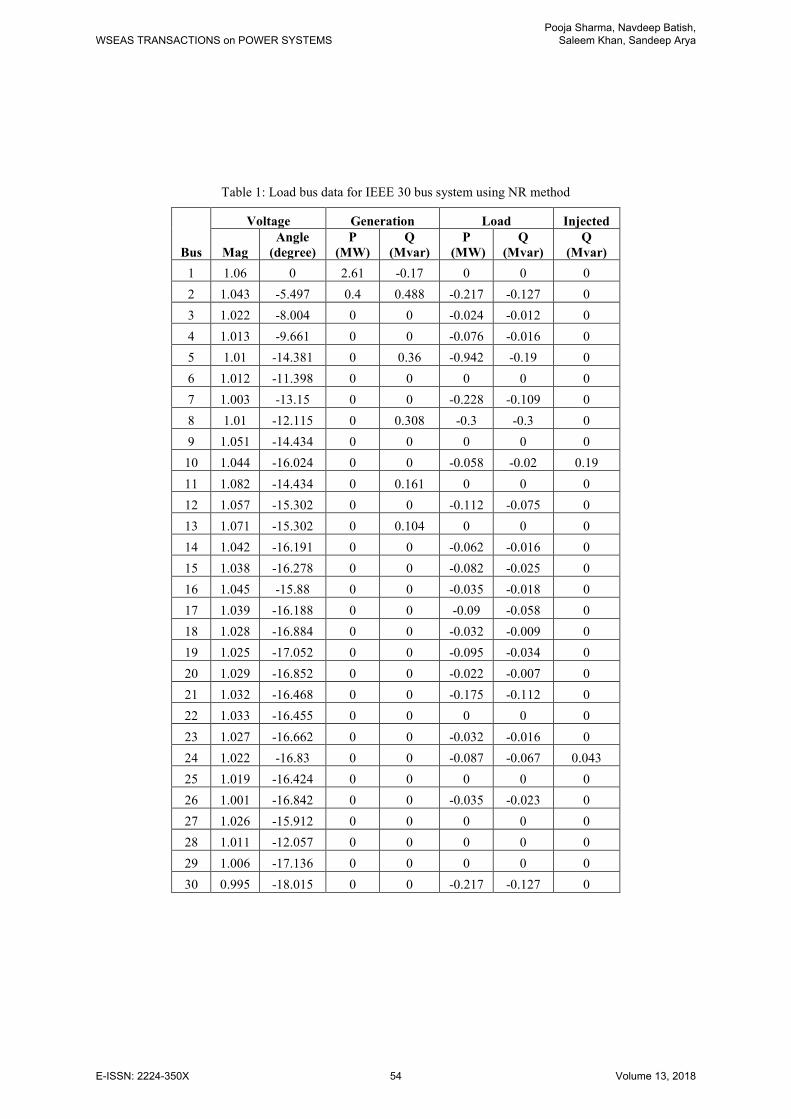
Table 1: Load bus data for IEEE 30 bus system using NR method

Bus

Voltage Generation Load Injected

Mag Angle

(degree) P

(MW) Q

(Mvar) P

(MW) Q

(Mvar) Q

(Mvar) 1 1.06 0 2.61 -0.17 0 0 0 2 1.043 -5.497 0.4 0.488 -0.217 -0.127 0 3 1.022 -8.004 0 0 -0.024 -0.012 0 4 1.013 -9.661 0 0 -0.076 -0.016 0 5 1.01 -14.381 0 0.36 -0.942 -0.19 0 6 1.012 -11.398 0 0 0 0 0 7 1.003 -13.15 0 0 -0.228 -0.109 0 8 1.01 -12.115 0 0.308 -0.3 -0.3 0 9 1.051 -14.434 0 0 0 0 0 10 1.044 -16.024 0 0 -0.058 -0.02 0.19 11 1.082 -14.434 0 0.161 0 0 0 12 1.057 -15.302 0 0 -0.112 -0.075 0 13 1.071 -15.302 0 0.104 0 0 0 14 1.042 -16.191 0 0 -0.062 -0.016 0 15 1.038 -16.278 0 0 -0.082 -0.025 0 16 1.045 -15.88 0 0 -0.035 -0.018 0 17 1.039 -16.188 0 0 -0.09 -0.058 0 18 1.028 -16.884 0 0 -0.032 -0.009 0 19 1.025 -17.052 0 0 -0.095 -0.034 0 20 1.029 -16.852 0 0 -0.022 -0.007 0 21 1.032 -16.468 0 0 -0.175 -0.112 0 22 1.033 -16.455 0 0 0 0 0 23 1.027 -16.662 0 0 -0.032 -0.016 0 24 1.022 -16.83 0 0 -0.087 -0.067 0.043 25 1.019 -16.424 0 0 0 0 0 26 1.001 -16.842 0 0 -0.035 -0.023 0 27 1.026 -15.912 0 0 0 0 0 28 1.011 -12.057 0 0 0 0 0 29 1.006 -17.136 0 0 0 0 0 30 0.995 -18.015 0 0 -0.217 -0.127 0



E-ISSN: 2224-350X 54 Volume 13, 2018

Table 2: Power losses for IEEE 30 bus system using NR method

Bus Bus Power flow

Power flow Power loss

nl nr nl to nr nr to nl P MW

Q Mvar

1 2 1.778+j-0.221 -1.723+j0.327 0.055 0.105

1 3 0.832+j0.051 -0.804+j0.02 0.028 0.071

2 4 0.457+j0.027 -0.446+j0.032 0.011 -0.005

3 4 0.780+j-0.032 -0.772+j0.045 0.008 0.013

2 5 0.830+j0.017 -0.8+j0.065 0.03 0.082

2 6 0.619+j-0.01 -0.599+j0.032 0.02 0.023

4 6 0.701+j-0.175 -0.695+j0.187 0.006 0.012

5 7 -0.142+j0.105 0.144+j-0.122 0.002 -0.017

6 7 0.375+j-0.019 -0.372+j0.013 0.004 -0.006

6 8 0.295+j-0.038 -0.294+j0.032 0.001 -0.006

6 9 0.277+j-0.297 -0.277+j0.331 0 0.034

6 10 0.158+j-0.113 -0.158+j0.134 0 0.021

9 11 -0+j-0.157 0.000+j0.161 0 0.005

9 10 0.277+j0.067 -0.277+j-0.059 0 0.008

4 12 0.441+j-0.46 -0.441+j0.561 0 0.101

12 13 -0+j-0.103 0.000+j0.104 0 0.001

12 14 0.079+j0.024 -0.078+j-0.023 0.001 0.002

12 15 0.179+j0.069 -0.176+j-0.065 0.002 0.004

12 16 0.072+j0.034 -0.072+j-0.033 0.001 0.001

14 15 0.016+j0.007 -0.016+j-0.007 0 0.000

16 17 0.037+j0.015 -0.036+j-0.014 0 0.000

15 18 0.060+j0.017 -0.06+j-0.017 0 0.001

18 19 0.028+j0.008 -0.028+j-0.008 0 0.000

19 20 -0.067+j-0.026 0.067+j0.027 0 0.000

10 20 0.090+j0.036 -0.089+j-0.034 0.001 0.002

10 17 0.054+j0.044 -0.054+j-0.044 0 0.000

10 21 0.157+j0.098 -0.156+j-0.096 0.001 0.002

10 22 0.076+j0.045 -0.075+j-0.044 0.001 0.001

21 22 -0.019+j-0.016 0.019+j0.016 0 0.000

15 23 0.050+j0.03 -0.05+j-0.029 0 0.001



E-ISSN: 2224-350X 55 Volume 13, 2018

Table 5: Optimal power flow results for IEEE 30 bus system using NR method

Bus Voltage Generation Load Lambda($/MVA-hr)

Mag(p.u) Ang(deg) P

(MW) Q

(Mvar) P

(MW) Q

(Mvar) P

(MW) Q

(Mvar)

1 0.982 0 41.54 -5.44 - - 3.662 -

2 0.979 -0.763 55.4 1.67 21.7 12.7 3.689 -

3 0.977 -2.39 - - 2.4 1.2 3.754 -0.016

4 0.976 -2.839 - - 7.6 1.6 3.771 -0.021

5 0.971 -2.486 - - - - 3.744 -0.001

6 0.972 -3.229 - - - - 3.779 -0.02

7 0.962 -3.491 - - 22.8 10.9 3.801 0.003

8 0.961 -3.682 - - 30 30 5.383 1.405

9 0.99 -4.137 - - - - 3.823 0.02

10 1 -4.6 - - 5.8 2 3.846 0.039

11 0.99 -4.137 - - - - 3.823 0.02

12 1.017 -4.498 - - 11.2 7.5 3.81 -

13 1.064 -3.298 16.2 35.93 - - 3.81 -

14 1.007 -5.04 - - 6.2 1.6 3.868 0.018

15 1.009 -4.814 - - 8.2 2.5 3.856 0.018

16 1.003 -4.839 - - 3.5 1.8 3.849 0.031

17 0.995 -4.887 - - 9 5.8 3.862 0.047

18 0.993 -5.484 - - 3.2 0.9 3.911 0.047

19 0.987 -5.688 - - 9.5 3.4 3.926 0.058

20 0.99 -5.472 - - 2.2 0.7 3.91 0.055

21 1.009 -4.621 - - 17.5 11.2 3.854 0.017

22 1.016 -4.503 22.74 34.2 - - 3.843 -

23 1.026 -3.756 16.27 6.96 3.2 1.6 3.813 -

24 1.017 -3.885 - - 8.7 6.7 3.884 0.028

25 1.044 -2.072 - - - - 3.932 0.022

26 1.027 -2.476 - - 3.5 2.3 3.999 0.067

27 1.069 -0.715 39.91 31.75 - - 3.916 -

28 0.982 -3.215 - - - - 4.106 0.25

29 1.05 -1.849 - - 2.4 0.9 3.966 -0.059

30 1.039 -2.643 - - 10.6 1.9 4.051 -0.012

Total: 192.06 105.08 189.2 107.2



E-ISSN: 2224-350X 56 Volume 13, 2018

Fig. 4: Graph showing losses as per active and reactive powers due to bus branches in IEEE 30 bus system.



E-ISSN: 2224-350X 57 Volume 13, 2018

5 Conclusion

In this paper, an IEEE 30 bus distribution system for optimal power flow is being discussed and studied. In this experiment, two methods were studied and compared, Newton Raphson (NR) method and Fast decoupled load flow (FDLF) method. Both studies showed almost same results. Moreover, power losses have also been evaluated for optimal conditions including power losses for this bus system. From the results, we can conclude that both methods are capable of obtaining optimum solution efficiently for Load flow problems. However, FDLF method converges than the NR method. The study was done using MATLAB simulation software and the results showed that FDLF method is more reliable and efficient than NR method. References: [1] B. Stott, “Review of load-flow calculation

methods,” in Proc. of IEEE, Vol. 62, p p. 916-929, 2005.

[2] H. Saadat, “Power System Analysis,” McGraw-Hill, New York, 1999.

[3] C. L. Wadhwa, “Electrical Power Systems”, New Age, New Delhi, 6th edition, 1983.

[4] W. F. Tinney and C. E Hart, “Power flow solution by Newton’s method,” IEEE Transactions on Power Systems PAS- 86, pp.1449-1456, 1967.

[5] R. Eid, S. W. Georges and R. A. Jabr, “Improved Fast Decoupled Power Flow,” Notre-Dame University, www.ndu.edu, retrieve, 2010.

[6] Puneet Sharma, Jyotsna Mehra, Virendra Kumar, “line flow analysis of IEEE bus system with load sensitivity factor,” in Proc. International Journal of Emerging Technology and Advanced Engineering, Vol. 4, Issue 5, pp. 899-903,2014.

[7] U. Thongkrajay, N. Poolsawat, T. RatniyomchaI & T. Kulworawanichpong, “Alternative Newton-Raphson Power Flow Calculation in Unbalanced Three-phase Power Distribution Systems,” in Proc. of the 5th WSEAS International Conference on Applications of Electrical Engineering, pp. 24-29, 2006.

[8] Wei-Tzer Huang and Wen-Chih Yang, “Power Flow Analysis of a Grid-Connected High Voltage Micro grid with Various Distributed Resources,” pp. 1471-1474, 2011.

[9] Idema, Reijer, Domenico Lahaye, Kees Vuik, and Lou van der Sluis, "Fast Newton load flow," In Transmission and Distribution Conference and Exposition, IEEE PES, pp. 1-7. IEEE, 2010.

[10] Vijay Kumar Shukla, Ashutosh Bhadoria, “Understanding Load Flow Studies by using PSAT,” International Journal of Enhanced Research in Science Technology & Engineering, Vol. 2 Issue 4, pp: 24-31, 2013.

[11] Jizhong Zhu,“ Optimization of Power system Operation,” Institute of Electrical and Electronics Engineers, Published by John Wiley & Sons, Inc., Hoboken, New Jersey. pp. 12-19, 2014.

[12] Nivedita Nayak, Dr. A.K. Wadhwani, “Performance of Newton-Raphson Techniques in Load Flow Analysis using MATLAB,” National Conference on Synergetic Trends in engineering and Technology, pp. 177-180, 2014.

[13] S. Iwamoto, IEEE Member, and Y. Tamura, Senior Member, IEEE, “A load flow calculation method for ill-conditioned power systems,” IEEE Transactions on Power Apparatus and Systems, Vol. PAS-100, No. 4, pp. 1736-1743, 1981.

[14] Khalid Mohamed Nor, Senior Member, IEEE, Hazlie Mokhlis, Member, IEEE, and Taufiq Abdul Gani, “Reusability Techniques in Load-Flow Analysis Computer Program,” IEEE transactions on power systems,, Vol. 19, pp.1754-1762, 2004.

[15] Ulas Eminoglu and M. Hakan Hocaoglu,“A new power flow method for radial distribution systems including voltage dependent load models,” Electric Power Systems Research, pp. 106-114, 2005.

[16] D. B. T. a. W. K. Lukman, "Loss Minimization in Industrial Power System Operation," in Proc. of the Australian Universities Power Engineering Conference(AUPEC'94), pp. 24-27, 2000.

[17] Jagabondhu Hazra and Avinash Kumar Sinha, “A New Power Flow Model Incorporating Effects of Automatic Controllers,” Wseas Transactions on POWER Systems, Issue 8, Vol. 2, pp. 202-207, 2007.

[18] K. Singh, “Fast decoupled for unbalanced radial distribution System,” Patiala: Thapar University, 2009.



E-ISSN: 2224-350X 58 Volume 13, 2018

[19] Aleksandar Dimitrovski, Member, IEEE, and Kevin Tomsovic, Senior Member, IEEE, “Boundary Load Flow Solutions,” IEEE Transactions on Power Systems, Vol. 19, No. 1, pp. 348-355, 2004.



E-ISSN: 2224-350X 59 Volume 13, 2018

power flow analysis for ieee 30 bus distribution system · load flow analysis. power flow analysis...

Documents