modelling and analysis of electric power systems€¦ · · 2012-04-25modelling and analysis of...
TRANSCRIPT
Modelling and Analysis of
Electric Power Systems
Power Flow Analysis
Fault Analysis
Power Systems Dynamics and Stability
Lecture 227-0526-00, ITET ETH Zurich
Goran AnderssonEEH - Power Systems Laboratory
ETH Zurich
September 2008

ii
Contents
Preface vii
I Static Analysis 1
1 Introduction 1
1.1 Power Flow Analysis . . . . . . . . . . . . . . . . . . . . . . . 1
1.2 Fault Current Analysis . . . . . . . . . . . . . . . . . . . . . . 3
1.3 Literature . . . . . . . . . . . . . . . . . . . . . . . . . . . . . 3
2 Network Models 5
2.1 Lines and Cables . . . . . . . . . . . . . . . . . . . . . . . . . 6
2.2 Transformers . . . . . . . . . . . . . . . . . . . . . . . . . . . 9
2.2.1 In-Phase Transformers . . . . . . . . . . . . . . . . . . 10
2.2.2 Phase-Shifting Transformers . . . . . . . . . . . . . . . 12
2.2.3 Unified Branch Model . . . . . . . . . . . . . . . . . . 14
2.3 Shunt Elements . . . . . . . . . . . . . . . . . . . . . . . . . . 16
2.4 Loads . . . . . . . . . . . . . . . . . . . . . . . . . . . . . . . 16
2.5 Generators . . . . . . . . . . . . . . . . . . . . . . . . . . . . 17
2.5.1 Stator Current Heating Limit . . . . . . . . . . . . . . 18
2.5.2 Field Current Heating Limit . . . . . . . . . . . . . . 19
2.5.3 Stator End Region Heating Limit . . . . . . . . . . . . 20
3 Active and Reactive Power Flows 21
3.1 Transmission Lines . . . . . . . . . . . . . . . . . . . . . . . . 21
3.2 In-phase Transformers . . . . . . . . . . . . . . . . . . . . . . 23
3.3 Phase-Shifting Transformer with akm = 1 . . . . . . . . . . . 24
3.4 Unified Power Flow Equations . . . . . . . . . . . . . . . . . . 25
4 Nodal Formulation of the Network Equations 27
5 Basic Power Flow Problem 31
5.1 Basic Bus Types . . . . . . . . . . . . . . . . . . . . . . . . . 31
5.2 Equality and Inequality Constraints . . . . . . . . . . . . . . 32
iii
iv Contents
5.3 Problem Solvability . . . . . . . . . . . . . . . . . . . . . . . . 34
6 Solution of the Power Flow Problem 37
6.1 Solution by Gauss-Seidel Iteration . . . . . . . . . . . . . . . 37
6.2 Newton-Raphson Method . . . . . . . . . . . . . . . . . . . . 39
6.2.1 Unidimensional case . . . . . . . . . . . . . . . . . . . 40
6.2.2 Quadratic Convergence . . . . . . . . . . . . . . . . . 41
6.2.3 Multidimensional Case . . . . . . . . . . . . . . . . . . 42
6.3 Newton-Raphson applied to the Power Flow Equations . . . . 44
6.4 Pθ − QU Decoupling . . . . . . . . . . . . . . . . . . . . . . . 45
6.5 Approximative Solutions of the Power Flow Problem . . . . . 48
6.5.1 Linearization . . . . . . . . . . . . . . . . . . . . . . . 48
6.5.2 Matrix Formulation of DC Power Flow Equations . . 52
6.5.3 DC Power Flow Model . . . . . . . . . . . . . . . . . . 55
7 Fault Analysis 57
7.1 Transients on a transmission line . . . . . . . . . . . . . . . . 61
7.2 Short circuit of a synchronous machine . . . . . . . . . . . . . 63
7.3 Algorithms for short circuit studies . . . . . . . . . . . . . . . 66
7.3.1 Generator model . . . . . . . . . . . . . . . . . . . . . 66
7.3.2 Simplifications . . . . . . . . . . . . . . . . . . . . . . 66
7.3.3 Solving the linear system equations . . . . . . . . . . . 67
7.3.4 The superposition technique . . . . . . . . . . . . . . . 68
7.3.5 The Takahashi method . . . . . . . . . . . . . . . . . . 71
II Power System Dynamics and Stability 77
8 Classification and Definitions of Power System Stability 79
8.1 Dynamics in Power Systems . . . . . . . . . . . . . . . . . . . 80
8.1.1 Classification of Dynamics . . . . . . . . . . . . . . . . 80
8.1.2 Modelling . . . . . . . . . . . . . . . . . . . . . . . . . 81
8.2 Power System Stability . . . . . . . . . . . . . . . . . . . . . . 82
8.2.1 Definition of Stability . . . . . . . . . . . . . . . . . . 82
8.2.2 Classification of Power System Stability . . . . . . . . 84
8.3 Literature on Power System Dynamics and Stability . . . . . 87
9 Synchronous Machine Models 89
9.1 Design and Operating Principle . . . . . . . . . . . . . . . . . 89
9.1.1 Rotor Types . . . . . . . . . . . . . . . . . . . . . . . 90
9.1.2 Stator Field . . . . . . . . . . . . . . . . . . . . . . . . 91
9.1.3 Magnetic Torque . . . . . . . . . . . . . . . . . . . . . 94
9.2 Stationary Operation . . . . . . . . . . . . . . . . . . . . . . . 95
9.2.1 Stationary Single Phase Equivalent Circuit . . . . . . 95
Contents v
9.2.2 Phasor diagram . . . . . . . . . . . . . . . . . . . . . . 97
9.2.3 Operational Limits . . . . . . . . . . . . . . . . . . . . 98
9.3 Dynamic Operation . . . . . . . . . . . . . . . . . . . . . . . 100
9.3.1 Transient Single Phase Equivalent Circuit . . . . . . . 100
9.3.2 Simplified Mechanical Model . . . . . . . . . . . . . . 100
10 The Swing Equation 103
10.1 Derivation of the Swing Equation . . . . . . . . . . . . . . . . 103
10.2 Analysis of the Swing Equation . . . . . . . . . . . . . . . . . 105
10.3 Swing Equation as System of First Order Differential Equations106
11 Power Swings in a Simple System 109
11.1 The Swing Equation and its Solutions . . . . . . . . . . . . . 109
11.1.1 Qualitative Analysis . . . . . . . . . . . . . . . . . . . 111
11.1.2 Stable and Unstable Solutions . . . . . . . . . . . . . . 113
11.2 Equal Area Criterion . . . . . . . . . . . . . . . . . . . . . . . 121
11.3 Lyapunov Stability Criterion . . . . . . . . . . . . . . . . . . 123
11.4 Small Signal Analysis . . . . . . . . . . . . . . . . . . . . . . 124
11.5 Methods to Improve System Stability . . . . . . . . . . . . . 127
12 Oscillations in Multi-Machine Systems 131
12.1 Simplified Model . . . . . . . . . . . . . . . . . . . . . . . . . 131
12.2 Detailed Model . . . . . . . . . . . . . . . . . . . . . . . . . . 132
13 Voltage Stability 135
13.1 Mechanisms of Voltage Instability . . . . . . . . . . . . . . . . 135
13.1.1 Long Term Voltage Instability . . . . . . . . . . . . . 136
13.1.2 Short Term Voltage Instability . . . . . . . . . . . . . 136
13.2 Simple Systems for Analysis of Voltage Stability . . . . . . . 137
13.3 Analysis of Voltage Stability . . . . . . . . . . . . . . . . . . . 140
13.3.1 Stability Indicators . . . . . . . . . . . . . . . . . . . . 141
13.3.2 Analysis of Simple System . . . . . . . . . . . . . . . . 142
14 Control of Electric Power Systems 151
14.1 Control of Active Power and Frequency . . . . . . . . . . . . 153
14.1.1 Spinning reserve . . . . . . . . . . . . . . . . . . . . . 154
14.1.2 Supplementary Reserves . . . . . . . . . . . . . . . . . 156
14.1.3 Back-Up Reserves . . . . . . . . . . . . . . . . . . . . 157
14.2 Control of Reactive Power and Voltage . . . . . . . . . . . . . 157
14.2.1 Reactive Power Control . . . . . . . . . . . . . . . . . 157
14.2.2 Voltage Control . . . . . . . . . . . . . . . . . . . . . . 158
14.3 Supervisory Control of Electric Power Systems . . . . . . . . 160
A Phase-Shifting Transformers 163

vi Contents
B Protections in Electric Power Systems 167B.1 Design of Protections . . . . . . . . . . . . . . . . . . . . . . . 167B.2 Distance Protections . . . . . . . . . . . . . . . . . . . . . . . 169
B.2.1 General Principles . . . . . . . . . . . . . . . . . . . . 169B.2.2 Automatic Re-Closure . . . . . . . . . . . . . . . . . . 171
B.3 Out of Step Protections . . . . . . . . . . . . . . . . . . . . . 172B.4 System Protections . . . . . . . . . . . . . . . . . . . . . . . . 172
Preface
These lectures notes are intended to be used in the Modellierung und Analyseelektrischer Netze (Vorlesungsnummer ETH Zurich 227-0526-00) lecturesgiven at ETH Zurich in Information Technology and Electrical Engineering.In the lectures three main topics are covered, i.e.
• Power flow analysis
• Fault current calculations
• Power systems dynamics and stability
In Part I of these notes the two first items are covered, while Part II givesan introduction to dynamics and stability in power systems. In appendicesbrief overviews of phase-shifting transformers and power system protectionsare given.
The notes start with a derivation and discussion of the models of the mostcommon power system components to be used in the power flow analysis.A derivation of the power flow equations based on physical considerations isthen given. The resulting non-linear equations are for realistic power systemsof very large dimension and they have to be solved numerically. The mostcommonly used techniques for solving these equations are reviewed. The roleof power flow analysis in power system planning, operation, and analysis isdiscussed.1
The next topic covered in these lecture notes is fault current calcula-tions in power systems. A systematic approach to calculate fault currentsin meshed, large power systems will be derived. The needed models will begiven and the assumptions made when formulating these models discussed.It will be demonstrated that algebraic models can be used to calculate thedimensioning fault currents in a power system, and the mathematical analy-sis has similarities with the power flow analysis, so it is natural to put thesetwo items in Part I of the notes.
In Part II the dynamic behaviour of the power system during and afterdisturbances (faults) will be studied. The concept of power system stabilityis defined, and different types of power system instabilities are discussed.While the phenomena in Part I could be studied by algebraic equations,
1As stated above, the presentation of the power flow problem is in these lecture notesbased on physical considerations. However, for implementation of these equations incomputer software, an object oriented approach is more suitable. Such an approach ispresented in the lecture notes Modellierung und Analyse elektrischer Netze, by RainerBacher, is also to be dealt with in the lectures. In those lecture notes the techniques forhandling large but sparse matrices are also reviewed.
vii

viii Preface
the description of the power system dynamics requires models based ondifferential equations.
These lecture notes provide only a basic introduction to the topics above.To facilitate for readers who want to get a deeper knowledge of and insightinto these problems, bibliographies are given in the text.
I want to thank numerous assistants, PhD students, and collaborators ofPower Systems Laboratory at ETH Zurich, who have contributed in variousways to these lecture notes.
Zurich, September 2008
Goran Andersson
Part I
Static Analysis
1

1Introduction
This chapter gives a motivation why an algebraic model can be used to de-scribe the power system in steady state. It is also motivated why an algebraicapproach can be used to calculate fault currents in a power system.
A POWER SYSTEM is predominantly in steady state operation or in astate that could with sufficient accuracy be regarded as steady state.
In a power system there are always small load changes, switching actions,and other transients occurring so that in a strict mathematical sense mostof the variables are varying with the time. However, these variations aremost of the time so small that an algebraic, i.e. not time varying model ofthe power system is justified.
A short circuit in a power system is clearly not a steady state condition.Such an event can start a variety of different dynamic phenomena in thesystem, and to study these dynamic models are needed. However, whenit comes to calculate the fault currents in the system, steady state (static)models with appropriate parameter values can be used. A fault currentconsists of two components, a transient part, and a steady state part, butsince the transient part can be estimated from the steady state one, faultcurrent analysis is commonly restricted to the calculation of the steady statefault currents.
1.1 Power Flow Analysis
It is of utmost importance to be able to calculate the voltages and currentsthat different parts of the power system are exposed to. This is essentialnot only in order to design the different power system components suchas generators, lines, transformers, shunt elements, etc. so that these canwithstand the stresses they are exposed to during steady state operationwithout any risk of damages. Furthermore, for an economical operation ofthe system the losses should be kept at a low value taking various constraintsinto account, and the risk that the system enters into unstable modes ofoperation must be supervised. In order to do this in a satisfactory way thestate of the system, i.e. all (complex) voltages of all nodes in the system,must be known. With these known, all currents, and hence all active and
1
2 1. Introduction
reactive power flows can be calculated, and other relevant quantities can becalculated in the system.
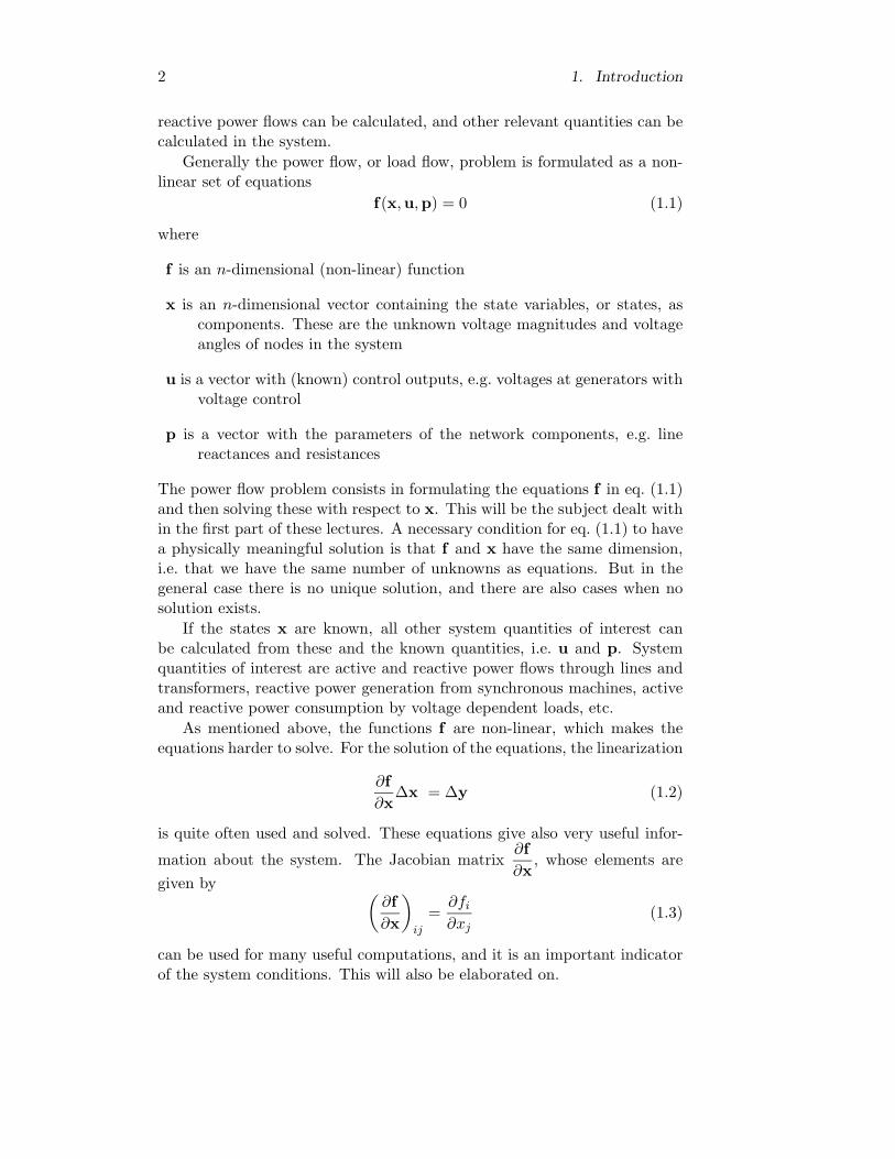
Generally the power flow, or load flow, problem is formulated as a non-linear set of equations
f(x,u,p) = 0 (1.1)
where
f is an n-dimensional (non-linear) function
x is an n-dimensional vector containing the state variables, or states, ascomponents. These are the unknown voltage magnitudes and voltageangles of nodes in the system
u is a vector with (known) control outputs, e.g. voltages at generators withvoltage control
p is a vector with the parameters of the network components, e.g. linereactances and resistances
The power flow problem consists in formulating the equations f in eq. (1.1)and then solving these with respect to x. This will be the subject dealt within the first part of these lectures. A necessary condition for eq. (1.1) to havea physically meaningful solution is that f and x have the same dimension,i.e. that we have the same number of unknowns as equations. But in thegeneral case there is no unique solution, and there are also cases when nosolution exists.
If the states x are known, all other system quantities of interest canbe calculated from these and the known quantities, i.e. u and p. Systemquantities of interest are active and reactive power flows through lines andtransformers, reactive power generation from synchronous machines, activeand reactive power consumption by voltage dependent loads, etc.
As mentioned above, the functions f are non-linear, which makes theequations harder to solve. For the solution of the equations, the linearization
∂f
∂x∆x = ∆y (1.2)
is quite often used and solved. These equations give also very useful infor-
mation about the system. The Jacobian matrix∂f
∂x, whose elements are
given by(
∂f
∂x
)
ij
=∂fi
∂xj(1.3)
can be used for many useful computations, and it is an important indicatorof the system conditions. This will also be elaborated on.
1.2. Fault Current Analysis 3
1.2 Fault Current Analysis
In the lectures Elektrische Energiesysteme it was studied how to calculatefault currents, e.g. short circuit currents, for simple systems. This analysiswill now be extended to deal with realistic systems including several gener-ators, lines, loads, and other system components. Generators (synchronousmachines) are important system components when calculating fault currentsand their modelling will be elaborated on and discussed.
1.3 Literature
The material presented in these lectures constitutes only an introductionto the subject. Further studies can be recommended in the following textbooks:
1. Power Systems Analysis, second edition, by Artur R. Bergen and VijayVittal. (Prentice Hall Inc., 2000, ISBN 0-13-691990-1, 619 pages)
2. Computational Methods for Large Sparse Power Systems, An objectoriented approach, by S.A. Soma, S.A. Khaparde, Shubba Pandit (KluwerAcademic Publishers, 2002, ISBN 0-7923-7591-2, 333 pages)

4 1. Introduction
2Network Models
In this chapter models of the most common network elements suitable forpower flow analysis are derived. These models will be used in the subsequentchapters when formulating the power flow problem.
ALL ANALYSIS in the engineering sciences starts with the formulationof appropriate models. A model, and in power system analysis we al-
most invariably then mean a mathematical model, is a set of equations orrelations, which appropriately describes the interactions between differentquantities in the time frame studied and with the desired accuracy of a phys-ical or engineered component or system. Hence, depending on the purposeof the analysis different models of the same physical system or componentsmight be valid. It is recalled that the general model of a transmission linewas given by the telegraph equation, which is a partial differential equation,and by assuming stationary sinusoidal conditions the long line equations,ordinary differential equations, were obtained. By solving these equationsand restricting the interest to the conditions at the ends of the lines, thelumped-circuit line models (π-models) were obtained, which is an algebraicmodel. This gives us three different models each valid for different purposes.
In principle, the complete telegraph equations could be used when study-ing the steady state conditions at the network nodes. The solution wouldthen include the initial switching transients along the lines, and the steadystate solution would then be the solution after the transients have decayed.However, such a solution would contain a lot more information than wantedand, furthermore, it would require a lot of computational effort. An alge-braic formulation with the lumped-circuit line model would give the sameresult with a much simpler model at a lower computational cost.
In the above example it is quite obvious which model is the appropriateone, but in many engineering studies the selection of the “correct” modelis often the most difficult part of the study. It is good engineering practiceto use as simple models as possible, but of course not too simple. If toocomplicated models are used, the analysis and computations would be un-necessarily cumbersome. Furthermore, generally more complicated modelsneed more parameters for their definition, and to get reliable values of theserequires often extensive work.
5
6 2. Network Models
u
dx
u+du
i+diR´dx L´dx
C´dxG´dx
i
Figure 2.1. Equivalent circuit of a line element of length dx
Figure 2.1. Equivalent circuit of a line element of length dx
In the subsequent sections algebraic models of the most common powersystem components suitable for power flow calculations will be derived. Ifnot explicitly stated, symmetrical three-phase conditions are assumed in thefollowing.
2.1 Lines and Cables
The equivalent π-model of a transmission line section was derived in thelectures Elektrische Energiesysteme, 35-505. The general distributed modelis characterized by the series parameters
R′ = series resistance/km per phase (Ω/km)
X ′ = series reactance/km per phase (Ω/km)
and the shunt parameters
B′ = shunt susceptance/km per phase (siemens/km)
G′ = shunt conductance/km per phase (siemens/km)
as depicted in Figure 2.1. The parameters above are specific for the lineor cable configuration and are dependent on conductors and geometricalarrangements.
From the circuit in Figure 2.1 the telegraph equation is derived, and fromthis the lumped-circuit line model for symmetrical steady state conditions,Figure 2.2. This model is frequently referred to as the π-model, and it ischaracterized by the parameters
Zkm = Rkm + jXkm = series impedance (Ω)
Y shkm = Gsh
km + jBshkm = shunt admittance (siemens) 1
1In Figure 2.2 the two shunt elements are assumed to be equal, which is true forhomogenous lines, i.e. a line with equal values of the line parameters along its length, butthis might not be true in the general case. In such a case the shunt elements are replacedby Y sh
km and Y shmk with Y sh
km 6= Y shmk with obvious notation.
2.1. Lines and Cables 7
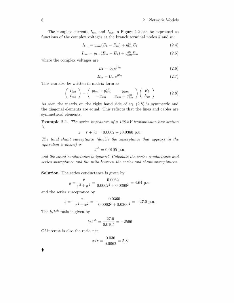
k m
kmz
shkmysh
kmy
kmI mkI
Figure 2.2. Lumped-circuit model (π-model) of a transmission linebetween nodes k and m.
Note. In the following most analysis will be made in the p.u. system. Forimpedances and admittances, capital letters indicate that the quantity is ex-pressed in ohms or siemens, and lower case letters that they are expressedin p.u.
Note. In these lecture notes complex quantities are not explicitly markedas underlined. This means that instead of writing zkm we will write zkm
when this quantity is complex. However, it should be clear from the contextif a quantity is real or complex. Furthermore, we will not always use specifictype settings for vectors. Quite often vectors will be denoted by bold face typesetting, but not always. It should also be clear from the context if a quantityis a vector or a scalar.
When formulating the network equations the node admittance matrixwill be used and the series admittance of the line model is needed
ykm = z−1km = gkm + jbkm (2.1)
withgkm =
rkm
r2km + x2
km
(2.2)
andbkm = − xkm
r2km + x2
km
(2.3)
For actual transmission lines the series reactance xkm and the seriesresistance rkm are both positive, and consequently gkm is positive and bkm
is negative. The shunt susceptance yshkm and the shunt conductance gsh
km areboth positive for real line sections. In many cases the value of gsh
km is sosmall that it could be neglected.
8 2. Network Models
The complex currents Ikm and Imk in Figure 2.2 can be expressed asfunctions of the complex voltages at the branch terminal nodes k and m:
Ikm = ykm(Ek − Em) + yshkmEk (2.4)
Imk = ykm(Em − Ek) + yshkmEm (2.5)
where the complex voltages are
Ek = Ukejθk (2.6)
Em = Umejθm (2.7)
This can also be written in matrix form as(
Ikm
Imk
)
=
(
ykm + yshkm −ykm
−ykm ykm + yshkm
)(
Ek
Em
)
(2.8)
As seen the matrix on the right hand side of eq. (2.8) is symmetric andthe diagonal elements are equal. This reflects that the lines and cables aresymmetrical elements.
Example 2.1. The series impedance of a 138 kV transmission line sectionis
z = r + jx = 0.0062 + j0.0360 p.u.
The total shunt susceptance (double the susceptance that appears in theequivalent π-model) is
bsh = 0.0105 p.u.
and the shunt conductance is ignored. Calculate the series conductance andseries susceptance and the ratio between the series and shunt susceptances.
Solution The series conductance is given by
g =r
r2 + x2=
0.0062
0.00622 + 0.03602= 4.64 p.u.
and the series susceptance by
b = − x
r2 + x2= − 0.0360
0.00622 + 0.03602= −27.0 p.u.
The b/bsh ratio is given by
b/bsh =−27.0
0.0105= −2596
Of interest is also the ratio x/r
x/r =0.036
0.0062= 5.8
2.2. Transformers 9
Example 2.2. The series impedance and the total shunt impedance of a750 kV line section are
z = r + jx = 0.00072 + j0.0175 p.u.
bsh = 8.77 p.u.
Calculate the series conductance and series susceptance and the ratio be-tween the series and shunt susceptances and the x/r ratio.
Solution The series conductance and susceptance are given by
g =0.00072
0.000722 + 0.01752= 2.35 p.u.
b = − 0.0175
0.000722 + 0.01752= −57 p.u.
The x/r ratio and b/bsh ratio are
x/r =0.0175
0.00072= 24.3
b/bsh =−57
8.77= −6.5
Note. The 750 kV line has a much higher x/r ratio than the 138 kV lineand, at the same time, a much smaller (in magnitude) b/bsh ratio. (Why?)Higher x/r ratios mean better decoupling between active and reactive partsof the power flow problem, while smaller (in magnitude) b/bsh ratios mayindicate the need for some sort of compensation, shunt or series, or both.
2.2 Transformers
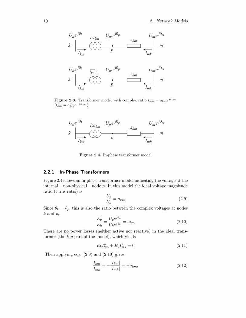
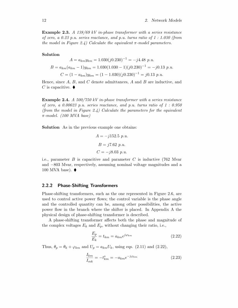
We will start with a simplified model of a transformer where we neglect themagnetizing current and the no-load losses 2. In this case the transformercan be modelled by an ideal transformer with turns ratio tkm in series witha series impedance zkm which represents resistive (load-dependent) lossesand the leakage reactance, see Figure 2.3. Depending on if tkm is real ornon-real (complex) the transformer is in-phase or phase-shifting.
2Often the magnetizing current and no-load losses are modelled by a shunt impedance,with much higher impedance than the leakage impedance. The inductive part of thisimpedance is then determined by the value of the magetizing current and the resistivepart by the no load losses.
10 2. Network Models
U ekjqk
U ekjqk
U emjqm
U emjqm
U epjqp
U epjqp
k
k
m
m
1 t: km
p
p
zkm
zkm
Imk
Imk
Ikm
Ikm
U ekjqk U em
jqmU epjqp
k mp
zkm
Imk
1 a: km
Ikm
k m
A
ImkIkm
CB
tkm:1
Figure 2.3. Transformer model with complex ratio tkm = akmejϕkm
(tkm = a−1
kme−jϕkm)
U ekjqk
U ekjqk
U emjqm
U emjqm
U epjqp
U epjqp
k
k
m
m
1 t: km
p
p
zkm
zkm
Imk
Imk
Ikm
Ikm
U ekjqk U em
jqmU epjqp
k mp
zkm
Imk
1 a: km
Ikm
k m
A
ImkIkm
CB
tkm:1
Figure 2.4. In-phase transformer model
2.2.1 In-Phase Transformers
Figure 2.4 shows an in-phase transformer model indicating the voltage at theinternal – non-physical – node p. In this model the ideal voltage magnituderatio (turns ratio) is
Up
Uk= akm (2.9)
Since θk = θp, this is also the ratio between the complex voltages at nodesk and p,
Ep
Ek=
Upejθp
Ukejθk= akm (2.10)
There are no power losses (neither active nor reactive) in the ideal trans-former (the k-p part of the model), which yields
EkI∗km + EpI
∗mk = 0 (2.11)
Then applying eqs. (2.9) and (2.10) gives
Ikm
Imk= −|Ikm|
|Imk|= −akm, (2.12)
2.2. Transformers 11
U ekjqk
U ekjqk
U emjqm
U emjqm
U epjqp
U epjqp
k
k
m
m
1 t: km
p
p
zkm
zkm
Imk
Imk
Ikm
Ikm
U ekjqk U em
jqmU epjqp
k mp
zkm
Imk
1 a: km
Ikm
k m
A
ImkIkm
CB
tkm:1
Figure 2.5. Equivalent π-model for in-phase transformer
which means that the complex currents Ikm and Imk are out of phase by180 since akm ∈ R.
Figure 2.5 represents the equivalent π-model for the in-phase transformerin Figure 2.4. Parameters A, B, and C of this model can be obtained byidentifying the coefficients of the expressions for the complex currents Ikm
and Imk associated with the models of Figures 2.4 and 2.5. Figure 2.4 gives
Ikm = −akmykm(Em − Ep) = (a2kmykm)Ek + (−akmykm)Em (2.13)
Imk = ykm(Em − Ep) = (−akmykm)Ek + (ykm)Em (2.14)
or in matrix form(
Ikm
Imk
)
=
(
a2kmykm −akmykm
−akmykm ykm
) (
Ek
Em
)
(2.15)
As seen the matrix on the right hand side of eq. (2.15) is symmetric, butthe diagonal elements are not equal when a2
km 6= 1. Figure 2.5 provides nowthe following:
Ikm = (A + B)Ek + (−A)Em (2.16)
Imk = (−A)Ek + (A + C)Em (2.17)
or in matrix form(
Ikm
Imk
)
=
(
A + B −A−A A + C
)(
Ek
Em
)
(2.18)
Identifying the matrix elements from the matrices in eqs. (2.15) and (2.18)yields
A = akmykm (2.19)
B = akm(akm − 1)ykm (2.20)
C = (1 − akm)ykm (2.21)
12 2. Network Models
Example 2.3. A 138/69 kV in-phase transformer with a series resistanceof zero, a 0.23 p.u. series reactance, and p.u. turns ratio of 1 : 1.030 (fromthe model in Figure 2.4) Calculate the equivalent π-model parameters.
SolutionA = akmykm = 1.030(j0.230)−1 = −j4.48 p.u.
B = akm(akm − 1)ykm = 1.030(1.030 − 1)(j0.230)−1 = −j0.13 p.u.
C = (1 − akm)ykm = (1 − 1.030)(j0.230)−1 = j0.13 p.u.
Hence, since A, B, and C denote admittances, A and B are inductive, andC is capacitive.
Example 2.4. A 500/750 kV in-phase transformer with a series resistanceof zero, a 0.00623 p.u. series reactance, and p.u. turns ratio of 1 : 0.950(from the model in Figure 2.4) Calculate the parameters for the equivalentπ-model. (100 MVA base)
Solution As in the previous example one obtains:
A = −j152.5 p.u.
B = j7.62 p.u.
C = −j8.03 p.u.
i.e., parameter B is capacitive and parameter C is inductive (762 Mvarand −803 Mvar, respectively, assuming nominal voltage magnitudes and a100 MVA base).
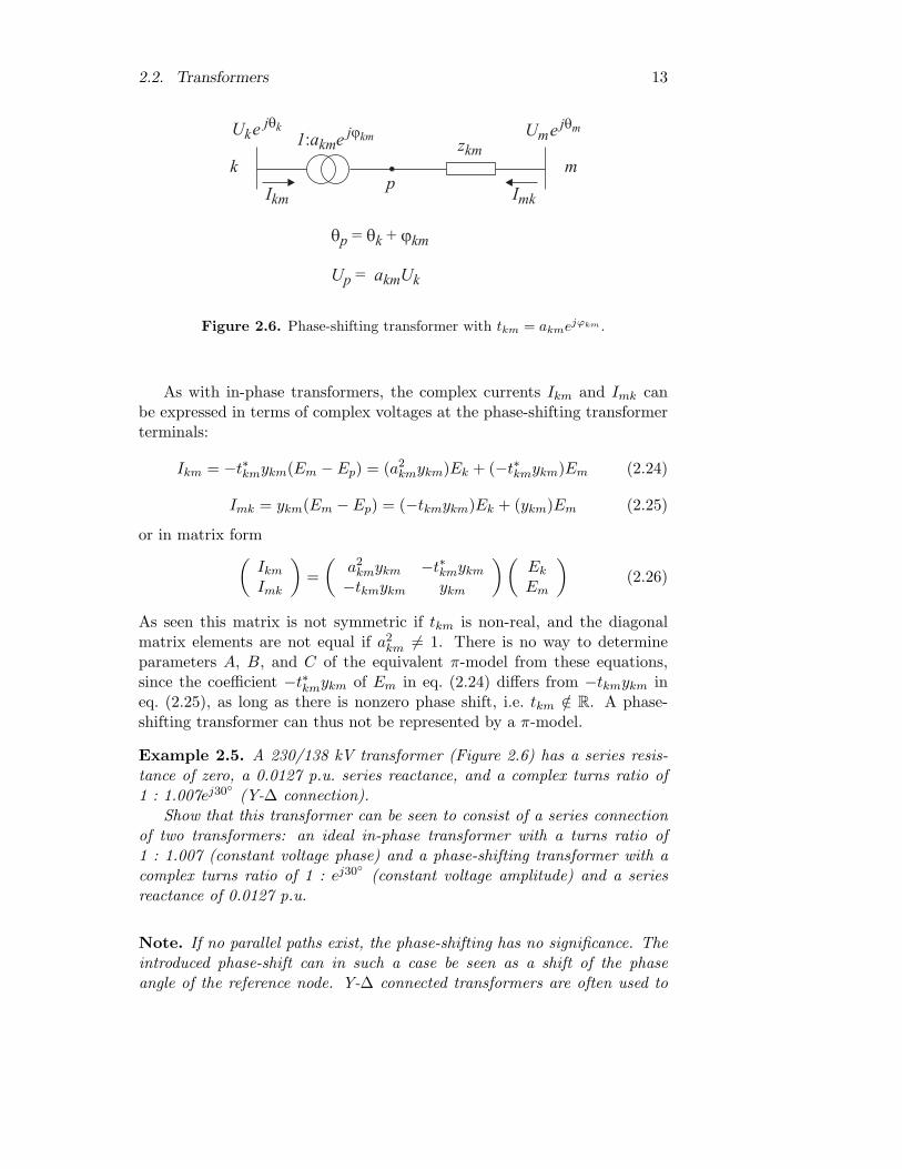
2.2.2 Phase-Shifting Transformers
Phase-shifting transformers, such as the one represented in Figure 2.6, areused to control active power flows; the control variable is the phase angleand the controlled quantity can be, among other possibilities, the activepower flow in the branch where the shifter is placed. In Appendix A thephysical design of phase-shifting transformer is described.
A phase-shifting transformer affects both the phase and magnitude ofthe complex voltages Ek and Ep, without changing their ratio, i.e.,
Ep
Ek= tkm = akmejϕkm (2.22)
Thus, θp = θk + ϕkm and Up = akmUk, using eqs. (2.11) and (2.22),
Ikm
Imk= −t∗km = −akme−jϕkm (2.23)
2.2. Transformers 13
U ekjqk
U ekjqk
U emjqm
U emjqmU ep
jqp U eqjqk
k
k
m
m
1 a: kmejjkm
1 t: km t 1mk:
p
p
zkm
zkm
Imk
Imk
Ikm
Ikm
q q jp k km= +
U a Up km k=
q
U epjqpU ek
jqk U eqjqq
k m
1 t: kmt 1mk:p zkm
ImkIkm
q
sh
kmy sh
mky
U emjqm
Figure 2.6. Phase-shifting transformer with tkm = akmejϕkm .
As with in-phase transformers, the complex currents Ikm and Imk canbe expressed in terms of complex voltages at the phase-shifting transformerterminals:
Ikm = −t∗kmykm(Em − Ep) = (a2kmykm)Ek + (−t∗kmykm)Em (2.24)
Imk = ykm(Em − Ep) = (−tkmykm)Ek + (ykm)Em (2.25)
or in matrix form(
Ikm
Imk
)
=
(
a2kmykm −t∗kmykm
−tkmykm ykm
) (
Ek
Em
)
(2.26)
As seen this matrix is not symmetric if tkm is non-real, and the diagonalmatrix elements are not equal if a2
km 6= 1. There is no way to determineparameters A, B, and C of the equivalent π-model from these equations,since the coefficient −t∗kmykm of Em in eq. (2.24) differs from −tkmykm ineq. (2.25), as long as there is nonzero phase shift, i.e. tkm /∈ R. A phase-shifting transformer can thus not be represented by a π-model.
Example 2.5. A 230/138 kV transformer (Figure 2.6) has a series resis-tance of zero, a 0.0127 p.u. series reactance, and a complex turns ratio of1 : 1.007ej30 (Y-∆ connection).
Show that this transformer can be seen to consist of a series connectionof two transformers: an ideal in-phase transformer with a turns ratio of1 : 1.007 (constant voltage phase) and a phase-shifting transformer with acomplex turns ratio of 1 : ej30 (constant voltage amplitude) and a seriesreactance of 0.0127 p.u.
Note. If no parallel paths exist, the phase-shifting has no significance. Theintroduced phase-shift can in such a case be seen as a shift of the phaseangle of the reference node. Y-∆ connected transformers are often used to
14 2. Network Models
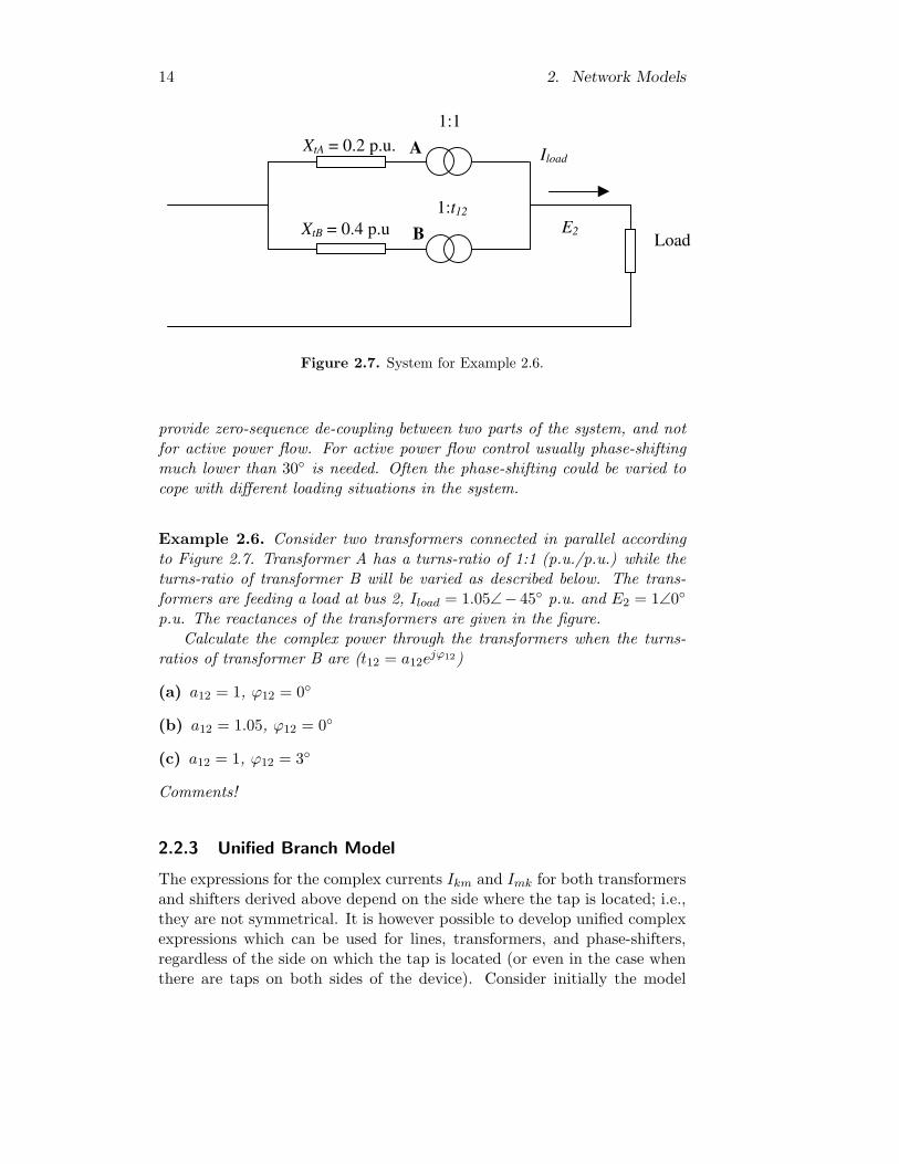
1:1
AIload
XtA = 0.2 p.u.
BE2
1:t12
XtB = 0.4 p.u Load
Figure 2.7. System for Example 2.6.
provide zero-sequence de-coupling between two parts of the system, and notfor active power flow. For active power flow control usually phase-shiftingmuch lower than 30 is needed. Often the phase-shifting could be varied tocope with different loading situations in the system.
Example 2.6. Consider two transformers connected in parallel accordingto Figure 2.7. Transformer A has a turns-ratio of 1:1 (p.u./p.u.) while theturns-ratio of transformer B will be varied as described below. The trans-formers are feeding a load at bus 2, Iload = 1.05∠− 45 p.u. and E2 = 1∠0
p.u. The reactances of the transformers are given in the figure.Calculate the complex power through the transformers when the turns-
ratios of transformer B are (t12 = a12ejϕ12)
(a) a12 = 1, ϕ12 = 0
(b) a12 = 1.05, ϕ12 = 0
(c) a12 = 1, ϕ12 = 3
Comments!
2.2.3 Unified Branch Model
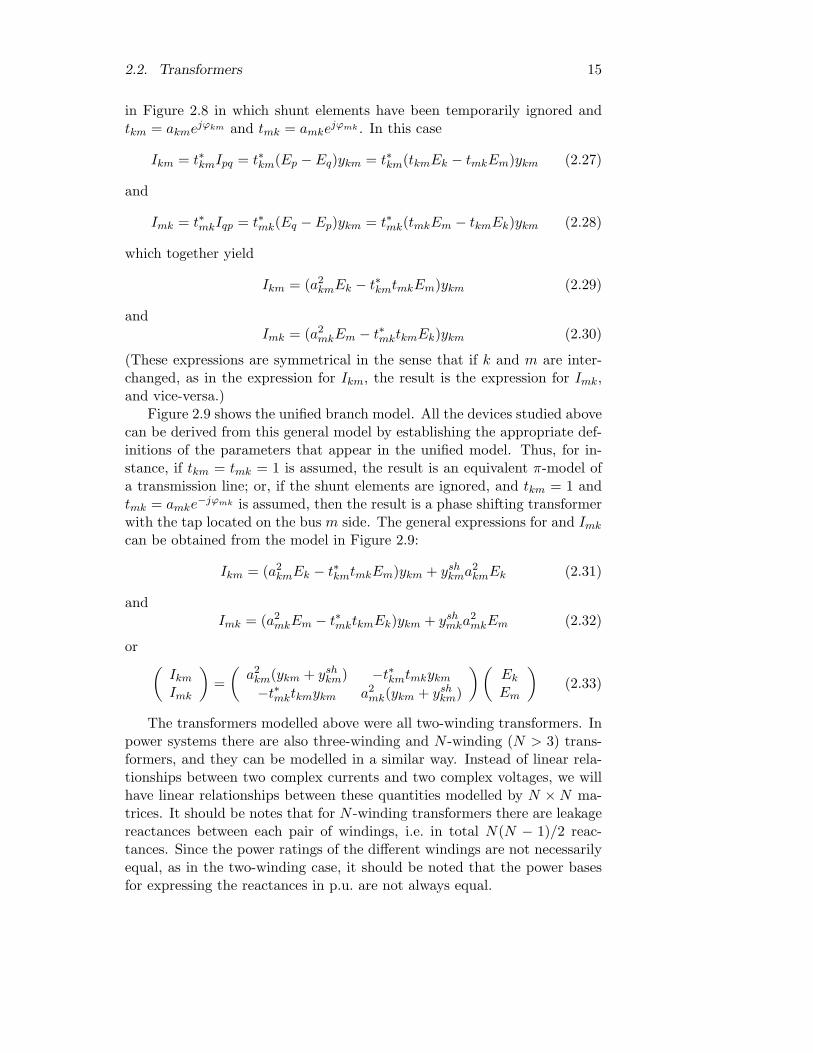
The expressions for the complex currents Ikm and Imk for both transformersand shifters derived above depend on the side where the tap is located; i.e.,they are not symmetrical. It is however possible to develop unified complexexpressions which can be used for lines, transformers, and phase-shifters,regardless of the side on which the tap is located (or even in the case whenthere are taps on both sides of the device). Consider initially the model
2.2. Transformers 15
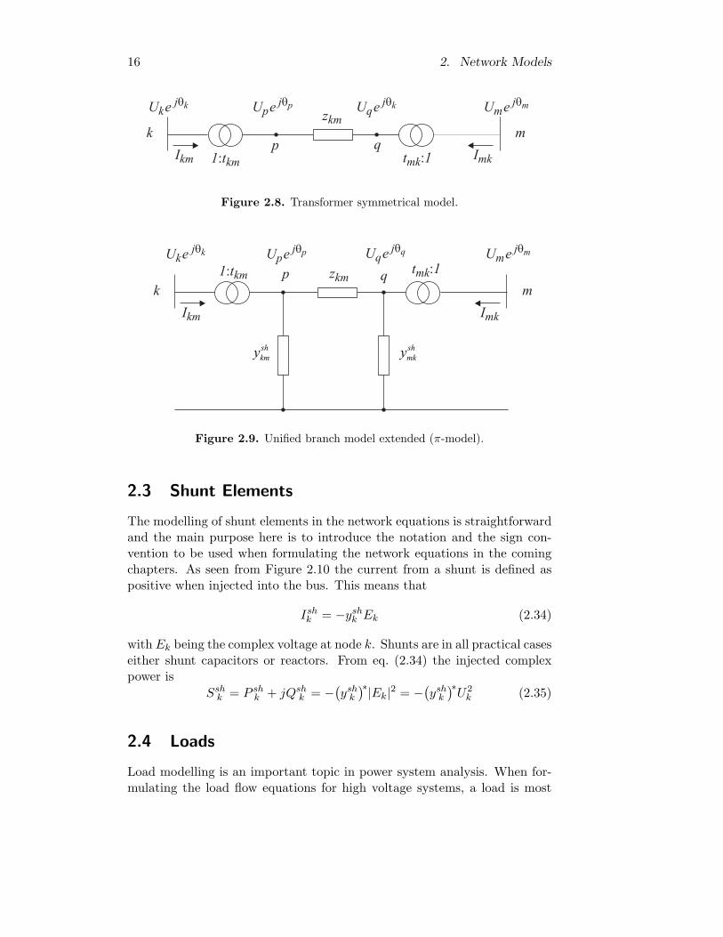
in Figure 2.8 in which shunt elements have been temporarily ignored andtkm = akmejϕkm and tmk = amke
jϕmk . In this case
Ikm = t∗kmIpq = t∗km(Ep − Eq)ykm = t∗km(tkmEk − tmkEm)ykm (2.27)
and
Imk = t∗mkIqp = t∗mk(Eq − Ep)ykm = t∗mk(tmkEm − tkmEk)ykm (2.28)
which together yield
Ikm = (a2kmEk − t∗kmtmkEm)ykm (2.29)
andImk = (a2
mkEm − t∗mktkmEk)ykm (2.30)
(These expressions are symmetrical in the sense that if k and m are inter-changed, as in the expression for Ikm, the result is the expression for Imk,and vice-versa.)
Figure 2.9 shows the unified branch model. All the devices studied abovecan be derived from this general model by establishing the appropriate def-initions of the parameters that appear in the unified model. Thus, for in-stance, if tkm = tmk = 1 is assumed, the result is an equivalent π-model ofa transmission line; or, if the shunt elements are ignored, and tkm = 1 andtmk = amke
−jϕmk is assumed, then the result is a phase shifting transformerwith the tap located on the bus m side. The general expressions for and Imk
can be obtained from the model in Figure 2.9:
Ikm = (a2kmEk − t∗kmtmkEm)ykm + ysh
kma2kmEk (2.31)
andImk = (a2
mkEm − t∗mktkmEk)ykm + yshmka
2mkEm (2.32)
or(
Ikm
Imk
)
=
(
a2km(ykm + ysh
km) −t∗kmtmkykm
−t∗mktkmykm a2mk(ykm + ysh
km)
)(
Ek
Em
)
(2.33)
The transformers modelled above were all two-winding transformers. Inpower systems there are also three-winding and N -winding (N > 3) trans-formers, and they can be modelled in a similar way. Instead of linear rela-tionships between two complex currents and two complex voltages, we willhave linear relationships between these quantities modelled by N × N ma-trices. It should be notes that for N -winding transformers there are leakagereactances between each pair of windings, i.e. in total N(N − 1)/2 reac-tances. Since the power ratings of the different windings are not necessarilyequal, as in the two-winding case, it should be noted that the power basesfor expressing the reactances in p.u. are not always equal.
16 2. Network Models
U ekjqk
U ekjqk
U emjqm
U emjqmU ep
jqp U eqjqk
k
k
m
m
1 a: kmejjkm
1 t: km t 1mk:
p
p
zkm
zkm
Imk
Imk
Ikm
Ikm
q q jp k km= +
U a Up km k=
q
U epjqpU ek
jqk U eqjqq
k m
1 t: kmt 1mk:p zkm
ImkIkm
q
sh
kmy sh
mky
U emjqm
Figure 2.8. Transformer symmetrical model.
U ekjqk
U ekjqk
U emjqm
U emjqmU ep
jqp U eqjqk
k
k
m
m
1 a: kmejjkm
1 t: km t 1mk:
p
p
zkm
zkm
Imk
Imk
Ikm
Ikm
q q jp k km= +
U a Up km k=
q
U epjqpU ek
jqk U eqjqq
k m
1 t: kmt 1mk:p zkm
ImkIkm
q
sh
kmy sh
mky
U emjqm
Figure 2.9. Unified branch model extended (π-model).
2.3 Shunt Elements
The modelling of shunt elements in the network equations is straightforwardand the main purpose here is to introduce the notation and the sign con-vention to be used when formulating the network equations in the comingchapters. As seen from Figure 2.10 the current from a shunt is defined aspositive when injected into the bus. This means that
Ishk = −ysh
k Ek (2.34)
with Ek being the complex voltage at node k. Shunts are in all practical caseseither shunt capacitors or reactors. From eq. (2.34) the injected complexpower is
Sshk = P sh
k + jQshk = −
(
yshk
)∗|Ek|2 = −(
yshk
)∗U2
k (2.35)
2.4 Loads
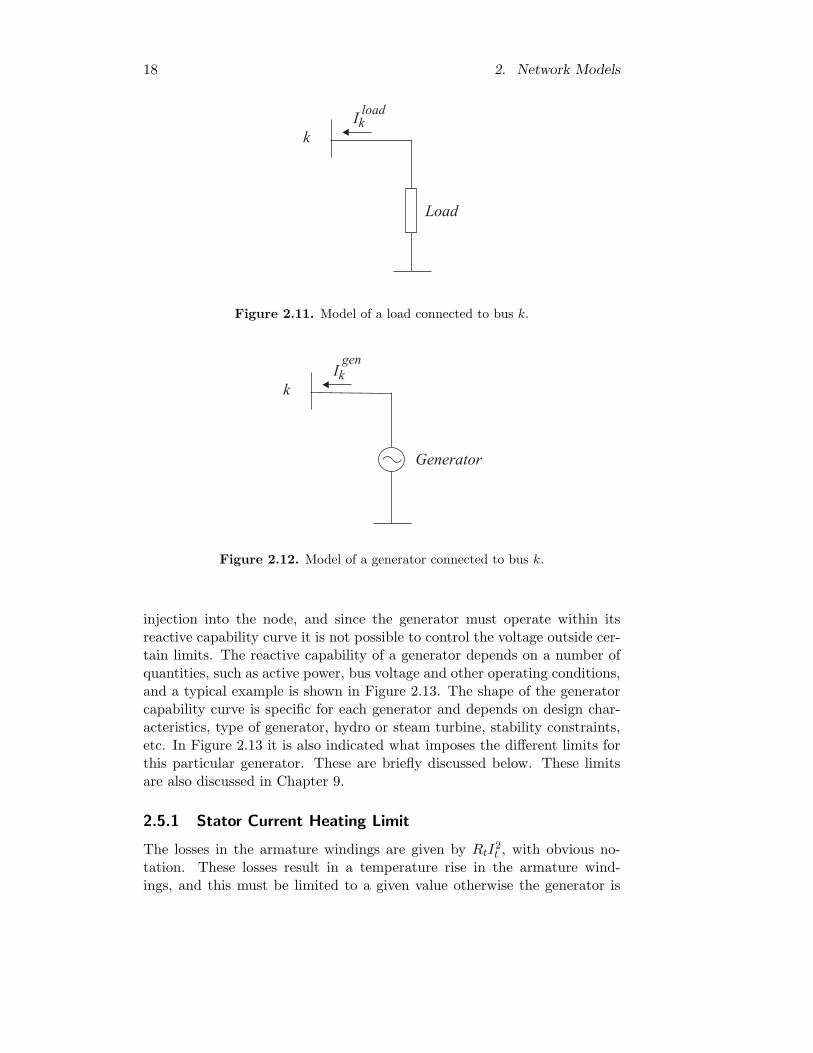
Load modelling is an important topic in power system analysis. When for-mulating the load flow equations for high voltage systems, a load is most
2.5. Generators 17
k
Iksh
Iksh
k
k
Ikload
Ik
gen
Load
Generator
Ik Ikm
yshk
yshk
Figure 2.10. A shunt connected to bus k.
often the infeed of power to a network at a lower voltage level, e.g. a dis-tribution network. Often the voltage in the distribution systems is keptconstant by controlling the tap-positions of the distribution transformerswhich means that power, active and reactive, in most cases can be regardedas independent of the voltage on the high voltage side. This means that thecomplex power Ek(I
loadk )∗ is constant, i.e. independent of the voltage mag-
nitude Uk. Also in this case the current is defined as positive when injectedinto the bus, see Figure 2.11. In the general case the complex load currentcan be written as
I loadk = I load
k (Uk) (2.36)
where the function I loadk (·) describes the load characteristics.3 More often
the load characteristics are given for the active and reactive powers
P loadk = P load
k (Uk) (2.37)
Qloadk = Qload
k (Uk) (2.38)
2.5 Generators
Generators are in load flow analysis modelled as current injections, see Fig-ure 2.12. In steady state a generator is commonly controlled so that theactive power injected into the bus and the voltage at the generator termi-nals are kept constant. This will be elaborated later when formulating theload flow equations. Active power from the generator is determined by theturbine control and must of course be within the capability of the turbine-generator system. Voltage is primarily determined by the reactive power
3This refers to the steady state model of the load. For transient conditions otherload models apply. These are usually formulated as differential equations and might alsoinvolve the frequency.
18 2. Network Models
k
Iksh
Iksh
k
k
Ikload
Ik
gen
Load
Generator
Ik Ikm
yshk
yshk
Figure 2.11. Model of a load connected to bus k.
k
Iksh
Iksh
k
k
Ikload
Ik
gen
Load
Generator
Ik Ikm
yshk
yshk
Figure 2.12. Model of a generator connected to bus k.
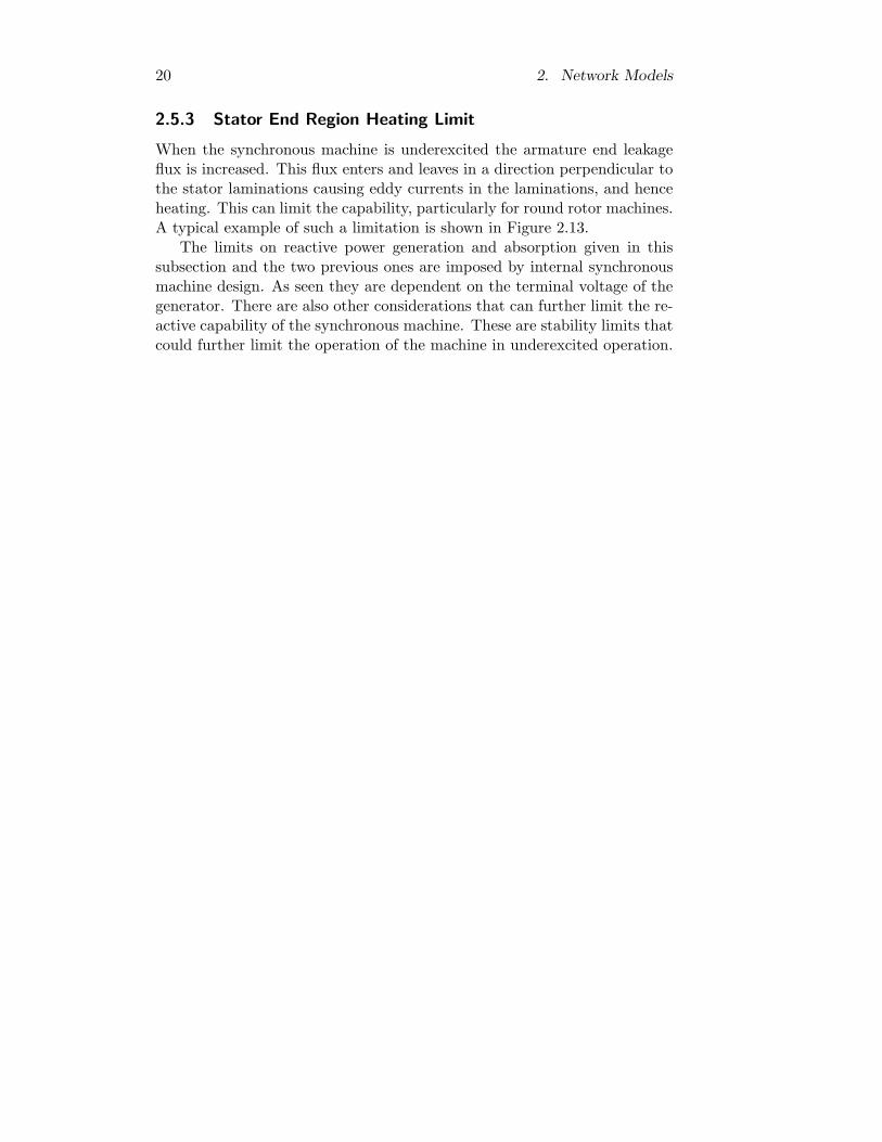
injection into the node, and since the generator must operate within itsreactive capability curve it is not possible to control the voltage outside cer-tain limits. The reactive capability of a generator depends on a number ofquantities, such as active power, bus voltage and other operating conditions,and a typical example is shown in Figure 2.13. The shape of the generatorcapability curve is specific for each generator and depends on design char-acteristics, type of generator, hydro or steam turbine, stability constraints,etc. In Figure 2.13 it is also indicated what imposes the different limits forthis particular generator. These are briefly discussed below. These limitsare also discussed in Chapter 9.
2.5.1 Stator Current Heating Limit
The losses in the armature windings are given by RtI2t , with obvious no-
tation. These losses result in a temperature rise in the armature wind-ings, and this must be limited to a given value otherwise the generator is

2.5. Generators 19
Q
P
Field currentheating limit
Stator currentheating limit
End regionheating limit
Under
exci
ted
Ove
rexc
ited
Figure 2.13. Reactive capability curve of a turbo generator.
damaged or its life time is reduced. Since the complex power is given byS = P + jQ = UtI
∗t it means that for a given terminal voltage, Ut, circles
in the P − Q-plane with centre at the origin correspond to constant valueof the magnitude of the armature current It. The stator current limit for agiven terminal voltage is thus a circle with the centre at the origin. At highloading of the generator, this is usually determining the reactive capabilityof the synchronous machine.
2.5.2 Field Current Heating Limit
The reactive power that can be generated at low load is determined by thefield current heating limit. It can be shown that the locus for constant fieldcurrent is a circle with the centre on the Q-axis at −E2
t /Xs, where Et is theterminal voltage and Xs is the synchronous reactance. The radius is givenby machine parameters and typical behaviour is shown in Figure 2.13. Thefield current heating is usually limiting at overexcited operation at low load.
20 2. Network Models
2.5.3 Stator End Region Heating Limit
When the synchronous machine is underexcited the armature end leakageflux is increased. This flux enters and leaves in a direction perpendicular tothe stator laminations causing eddy currents in the laminations, and henceheating. This can limit the capability, particularly for round rotor machines.A typical example of such a limitation is shown in Figure 2.13.
The limits on reactive power generation and absorption given in thissubsection and the two previous ones are imposed by internal synchronousmachine design. As seen they are dependent on the terminal voltage of thegenerator. There are also other considerations that can further limit the re-active capability of the synchronous machine. These are stability limits thatcould further limit the operation of the machine in underexcited operation.
3Active and Reactive Power Flows
In this chapter the expressions for the active and reactive power flows intransmission lines, transformers, phase-shifting transformers, and unifiedbranch models are derived.
THE SYSTEM COMPONENTS dealt with in this chapter are linear inthe sense that the relations between voltages and currents are linear1.
However, since one usually is interested rather in powers, active and reactive,than currents, the resulting equations will be non-linear, which introducesa complication when solving the resulting equations.
3.1 Transmission Lines
Consider the complex current Ikm in a transmission line
Ikm = ykm(Ek − Em) + jbshkmEk (3.1)
with quantities defined according to Figure 2.2. The complex power, Skm =Pkm + jQkm, is
Skm = EkI∗km = y∗kmUke
jθk(Uke−jθk − Ume−jθm) − jbsh
kmU2k (3.2)
where the conductance of yshkm has been neglected.
The expressions for Pkm and Qkm can be determined by identifying thecorresponding coefficients of the real and imaginary parts of eq. (3.2), whichyields
Pkm = U2kgkm − UkUmgkm cos θkm − UkUmbkm sin θkm (3.3)
Qkm = −U2k (bkm + bsh
km) + UkUmbkm cos θkm − UkUmgkm sin θkm (3.4)
where the notation θkm = θk − θm is introduced.
1This is at least true for the models analysed here. Different non-linear phenomena,e.g. magnetic saturation, can sometimes be important, but when studying steady stateconditions the devices to be discussed in this chapter are normally within the region oflinearity.
21
22 3. Active and Reactive Power Flows
The active and reactive power flows in opposite directions, Pmk and Qmk,can be obtained in the same way, resulting in:
Pmk = U2mgkm − UkUmgkm cos θkm + UkUmbkm sin θkm (3.5)
Qmk = −U2m(bkm + bsh
km) + UkUmbkm cos θkm + UkUmgkm sin θkm (3.6)
From these expressions the active and reactive power losses of the linesare easily obtained as:
Pkm + Pmk = gkm(U2k + U2
m − 2UkUm cos θkm)
= gkm|Ek − Em|2 (3.7)
Qkm + Qmk = −bshkm(U2
k + U2m) − bkm(U2
k + U2m − 2UkUm cos θkm)
= −bshkm(U2
k + U2m) − bkm|Ek − Em|2 (3.8)
Note that |Ek −Em| represents the magnitude of the voltage drop acrossthe line, gkm|Ek −Em|2 represents the active power losses, −bsh
km|Ek −Em|2represents the reactive power losses; and −bsh
km(U2k + U2
m) represents thereactive power generated by the shunt elements of the equivalent π-model(assuming actual transmission line sections, i.e. with bkm < 0 and bsh
km > 0).
Example 3.1. A 750 kV transmission line section has a series impedanceof 0.00072 + j0.0175 p.u., a total shunt impedance of 8.775 p.u., a voltagemagnitude at the terminal buses of 0.984 p.u. and 0.962 p.u., and a voltageangle difference of 22. Calculate the active and reactive power flows.
Solution The active and reactive power flows in the line are obtained byapplying eqs. (3.3) and (3.4), where Uk = 0.984 p.u., Um = 0.962 p.u., andθkm = 22. The series impedance and admittances are as follows:
zkm = 0.00072 + j0.0175 p.u.
ykm = gkm + jbkm = z−1km = 2.347 − j57.05 p.u.
The π-model shunt admittances (100 MVA base) are:
bshkm = 8.775/2 = 4.387 p.u.
and
Pkm = 0.9842·2.347−0.984·0.962·2.347 cos 22+00.984·0.962·57.05 sin 22 p.u.
Qkm = −0.9842·(−57.05+4.39)−0.984·0.962·57.05 cos 22−00.984·0.962·2.347 sin 22 p.u.
which yieldPkm = 2044 MW Qkm = 8.5 Mvar
3.2. In-phase Transformers 23
In similar way one obtains:
Pmk = −2012 MW Qmk = −50.5 Mvar
It should be noted that powers are positive when injected into the line.
3.2 In-phase Transformers
The complex current Ikm in an in-phase transformer is expressed as ineq. (2.13)
Ikm = akmykm(akmEk − Em)
The complex power, Skm = Pkm + jQkm, is given by
Skm = EkI∗km = y∗kmakmUke
jθk(akmUke−jθk − Ume−jθm) (3.9)
Separating the real and imaginary parts of this latter expression yieldsthe active and reactive power flow equations:
Pkm = (akmUk)2gkm − akmUkUmgkm cos θkm − akmUkUmbkm sin θkm
(3.10)
Qkm = −(akmUk)2bkm + akmUkUmbkm cos θkm − akmUkUmgkm sin θkm
(3.11)
These same expressions can be obtained by comparing eqs. (3.9) and(3.2); in eq. (3.9) the term jbsh
kmU2k is not present, and Uk is replaced by
akmUk. Hence, the expressions for the active and reactive power flows onin-phase transformers are the same expressions derived for a transmissionline, except the for two modifications: ignore bsh
km, and replace Uk withakmUk.
Example 3.2. A 500/750 kV transformer with a tap ratio of 1.050:1.0on the 500 kV side, see Figure 2.4, has negligible series resistance and aleakage reactance of 0.00623 p.u., terminal voltage magnitudes of 1.023 p.u.and 0.968 p.u., and an angle spread of 5.3. Calculate the active and reactivepower flows in the transformer.
Solution The active and reactive power flows in the transformer are givenby eqs. (3.10) and (3.11), where Uk = 1.023 p.u., Um = 0.968 p.u., θkm =5.3, and akm = 1.0/1.05 = 0.9524. The series reactance and susceptanceare as follows:
xkm = 0.00623 p.u.
bkm = −x−1km = −160.51 p.u.
24 3. Active and Reactive Power Flows
The active and reactive power flows can be expressed as
Pkm = −0.9524 · 1.023 · 0.968 · (−160.51) sin 5.3 p.u.
Qkm = −(0.9524·1.023)2(−160.51)+0.9524·1.023·0.968·(−160.51) cos 5.3 p.u.
which yield
Pkm = 1398 MW Qkm = 163 Mvar
The reader is encouraged to calculate Pmk and Qmk. (The value of Pmk
should be obvious.)
3.3 Phase-Shifting Transformer with akm = 1
The complex current Ikm in a phase shifting transformer with akm = 1 is asfollows, see Figure 2.6:
Ikm = ykm(Ek − e−jϕkmEm) = ykme−jϕkm(Ekejϕkm − Em) (3.12)
and the complex power, Skm = Pkm + jQkm, is thus
Skm = EkI∗km = y∗kmUke
j(θk+ϕkm)(Uke−j(θk+ϕkm) − Ume−jθm) (3.13)
Separating the real and imaginary parts of this expression, yields theactive and reactive power flow equations, respectively:
Pkm = U2kgkm − UkUmgkm cos(θkm + ϕkm)
− UkUmbkm sin(θkm + ϕkm) (3.14)
Qkm = −U2k bkm + UkUmbkm cos(θkm + ϕkm)
− UkUmgkm sin(θkm + ϕkm) (3.15)
As with in-phase transformers, these expressions could have been ob-tained through inspection by comparing eqs. (3.2) and (3.13): in eq. (3.13),the term jbsh
kmU2k is not present, and θkm is replaced with θkm +ϕkm. Hence,
the expressions for the active and reactive power flows in phase-shiftingtransformers are the same expressions derived for the transmission line, al-beit with two modifications: ignore bsh
km and replace θkm with θkm + ϕkm.
Example 3.3. A ∆-Y , 230/138 kV transformer presents a 30 phase an-gle shift. Series resistance is neglected and series reactance is 0.0997 p.u.Terminal voltage magnitudes are 0.882 p.u. and 0.989 p.u., and the totalangle difference is −16.6. Calculate the active and reactive power flows inthe transformer.
3.4. Unified Power Flow Equations 25
Solution The active and reactive power flows in the phase-shifting trans-former are given by eqs. (3.14) and (3.15), where Uk = 0.882 p.u., Um =0.989 p.u., θkm = −16.6, and ϕkm = 30. The series reactance and suscep-tance are as follows:
xkm = 0.0997 p.u.
bkm = −x−1km = −10.03 p.u.
The active and reactive power flows can be expressed as
Pkm = −0.882 · 0.989 · (−10.03) · (−160.51) sin(−16.6 + 30) p.u.
Qkm = −0.8822(−10.03) + 0.882 · 0.989 · (−10.03) cos(−16.6 + 30) p.u.
which yieldPkm = 203 MW Qkm = −70.8 Mvar
The reader is encouraged to calculate Pmk and Qmk. (The value of Pmk
should be obvious.)
3.4 Unified Power Flow Equations
The expressions for active and reactive power flows on transmission lines,in-phase transformers, and phase shifting transformers, see Figure 2.9, canbe expressed in the following unified forms:
Pkm = (akmUk)2gkm
− (akmUk)(amkUm)gkm cos(θkm + ϕkm − ϕmk)
− (akmUk)(amkUm)bkm sin(θkm + ϕkm − ϕmk) (3.16)
Qkm = (akmUk)2(bkm + bsh
km)
+ (akmUk)(amkUm)bkm cos(θkm + ϕkm − ϕmk)
− (akmUk)(amkUm)gkm sin(θkm + ϕkm − ϕmk) (3.17)
Where, for the transmission lines like the one represented in Figure 2.2,akm = amk = 1 and ϕkm = ϕmk = 0; for in-phase transformers such as theone represented in Figure 2.4, ysh
km = yshmk = 0, amk = 1 and ϕkm = ϕmk = 0;
and for a phase-shifting transformer such as the one in Figure 2.6, yshkm =
yshmk = 0, amk = 1 and ϕmk = 0.

26 3. Active and Reactive Power Flows
4Nodal Formulation of the Network Equa-
tions
In this chapter the basic network equations are derived from Kirchhoff’sCurrent Law (KCL) and put into forms that are suitable for the formulationof the power flow equations in the subsequent chapter
THE NET COMPLEX current injection at a network bus, see Figure 4.1,is related to the current flows in the branches connected to the bus.
Applying Kirchhoff’s Current Law (KCL) yields
Ik + Ishk =
∑
m∈Ωk
Ikm, for k = 1, . . . , N (4.1)
where k is a generic node, Ik is the net current injection from generatorsand loads, Ish
k is the current injection from shunts, m is a node adjacent tok, Ωk is the set of nodes adjacent to k, and N is the number of nodes in thenetwork.
The complex current Ikm in the unified branch model, Figure 2.9, is
Ikm = (a2kmEk − t∗kmtmkEm)ykm + ysh
kma2kmEk (4.2)
where tkm = akmejϕkm and tmk = amkejϕmk .
k
Iksh
Iksh
k
k
Ikload
Ik
gen
Load
Generator
Ik Ikm
yshk
yshk
Figure 4.1. Generic bus with sign conventions for currents and power flows.
27
28 4. Nodal Formulation of the Network Equations
Equations (4.1) and (4.2) yield
Ik =(
yshk +
∑
m∈Ωk
a2km(ysh
km + ykm))
Ek −∑
m∈Ωk
(t∗kmtmkykm)Em (4.3)
for k = 1, . . . , N . This expression can be written as
I = YE (4.4)
where
• I is the injection vector with elements Ik, k = 1, . . . , N
• E is the nodal voltage vector with elements Ek = Ukejθk
• Y = G + jB is the nodal admittance matrix, with the following ele-ments
Ykm = −t∗kmtmkykm (4.5)
Ykk = yshk +
∑
m∈Ωk
a2km(ysh
km + ykm) (4.6)
We see that the nodal admittance matrix defined by eqs. (4.5) and (4.6)is modified as compared with the nodal admittance matrix without trans-formers. Particularly it should be noted that Y as defined above is notnecessarily symmetric.
For large practical networks this matrix is usually very sparse. Thedegree of sparsity (percentage of zero elements) normally increases withthe dimensions of the network: e.g., a network with 1000 buses and 1500branches typically presents a degree of sparsity greater than 99 %, i.e. lessthan 1 % of the matrix elements have non-zero values.
The kth component of I, Ik, defined in eq. (4.3), can, by using eqs. (4.5)and (4.6), be written as
Ik = YkkEk +∑
m∈Ωk
YkmEm =∑
m∈K
YkmEm (4.7)
where K is the set of buses adjacent to bus k, including bus k, and Ωk isthe set of buses adjacent to bus k, excluding bus k. Now considering thatYkm = Gkm + jBkm and Em = Umejθm , eq. (4.7) can be rewritten as
Ik =∑
m∈K
(Gkm + jBkm)(Umejθm) (4.8)
The complex power injection at bus k is
Sk = Pk + jQk = EkI∗k (4.9)
29
and by applying eqs. (4.8) and (4.9) this gives
Sk = Ukejθk
∑
m∈K
(Gkm − jBkm)(Ume−jθm) (4.10)
The expressions for active and reactive power injections are obtained byidentifying the real and imaginary parts of eq. (4.10), yielding
Pk = Uk
∑
m∈K
Um(Gkm cos θkm + Bkm sin θkm) (4.11)
Qk = Uk
∑
m∈K
Um(Gkm sin θkm − Bkm cos θkm) (4.12)

30 4. Nodal Formulation of the Network Equations
5Basic Power Flow Problem
In this chapter the basic power flow problem is formulated and the basicbus types are defined. Also, the conditions for solvability of the problem arediscussed
THE POWER FLOW PROBLEM can be formulated as a set of non-linear algebraic equality/inequality constraints. These constraints rep-
resent both Kirchhoff’s laws and network operation limits. In the basicformulation of the power flow problem, four variables are associated to eachbus (network node) k:
• Uk: voltage magnitude
• θk: voltage angle
• Pk: net active power (algebraic sum of generation and load)
• Qk: net reactive power (algebraic sum of generation and load)
5.1 Basic Bus Types
Depending on which of the above four variables are known (given) and whichones are unknown (to be calculated), two basic types of buses can be defined:
• PQ bus: Pk and Qk are specified; Uk and θk are calculated
• PU bus: Pk and Uk are specified; Qk and θk are calculated
PQ buses are normally used to represent load buses without voltage control,and PU buses are used to represent generation buses with voltage controlin power flow calculations1. Synchronous compensators2 are also treated asPU buses. A third bus is also needed:
1Synchronous machines are often equipped with Automatic Voltage Regulators (AVRs),which controls the excitation of the machine so that the terminal voltage, or some othervoltage close to the machine, is kept at the set value.
2Synchronous compensators, sometimes also called synchronous condensers, are syn-chronous machines without any active power generation or load (except for losses) usedfor reactive power and voltage control.
31
32 5. Basic Power Flow Problem
• Uθ bus: Uk and θk are specified; Pk and Qk are calculated
The Uθ bus, also called reference bus or slack bus, has double functions inthe basic formulation of the power flow problem:
1. It serves as the voltage angle reference
2. Since the active power losses are unknown in advance, the active powergeneration of the Uθ bus is used to balance generation, load, and losses
In “normal” power systems PQ-buses or load buses are the far most common,typically comprising more than 80% of all buses.
Other possible bus types are P, U, and PQU, with obvious definitions.The use of multiple Uθ buses may also be required for certain applications.In more general cases, the given values are not limited to the specific set ofbuses (P, Q, U, θ), and branch related variables can also be specified.
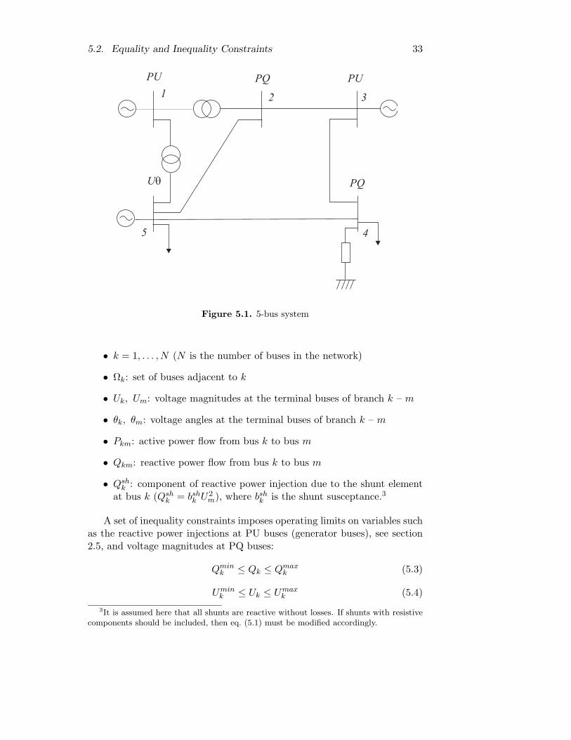
Example 5.1. Figure 5.1 shows a 5-bus network with four transmissionlines and two transformers. Generators, with voltage control, are connectedat buses 1, 3, and 5, and loads are connected at buses 4 and 5, and at bus 4a shunt is also connected. Classify the buses according to the bus types PU,PQ and Uθ.
Solution Buses 1, 3, and 5 are all candidates for PU or Uθ bus types. Sinceonly one could be Uθ bus, we select (arbitrarily) bus 5 as Uθ. In a practicalsystem usually a generator, or generator station, that could produce powerwithin a large range is selected as reference or slack bus. It should be notedthat even if a load is connected to bus 5 it can only be a PU or Uθ bus, sincevoltage control is available at the bus. The reference angle is set at bus 5,usually to 0. Bus 2 is a transition bus in which both P and Q are equal tozero, and this bus is consequently of type PQ. Bus 4 is a load bus to whichis also connected a shunt susceptance: since shunts are modelled as part ofthe network, see next section, the bus is also classified as a PQ bus.
5.2 Equality and Inequality Constraints
Eqs. (4.11) and (4.12) can be rewritten as follows
Pk =∑
m∈Ωk
Pkm(Uk, Um, θk, θm) (5.1)
Qk + Qshk (Uk) =
∑
m∈Ωk
Qkm(Uk, Um, θk, θm) (5.2)
where
5.2. Equality and Inequality Constraints 33
k mrkm + jxkm
jb jbkm km
sh sh (a)
k
(b)
mxkm
Pkm mk= (q - q ) xkm
PU PQ
PQUq
PU
1 2 3
45
Figure 5.1. 5-bus system
• k = 1, . . . , N (N is the number of buses in the network)
• Ωk: set of buses adjacent to k
• Uk, Um: voltage magnitudes at the terminal buses of branch k – m
• θk, θm: voltage angles at the terminal buses of branch k – m
• Pkm: active power flow from bus k to bus m
• Qkm: reactive power flow from bus k to bus m
• Qshk : component of reactive power injection due to the shunt element
at bus k (Qshk = bsh
k U2m), where bsh
k is the shunt susceptance.3
A set of inequality constraints imposes operating limits on variables suchas the reactive power injections at PU buses (generator buses), see section2.5, and voltage magnitudes at PQ buses:
Qmink ≤ Qk ≤ Qmax
k (5.3)
Umink ≤ Uk ≤ Umax
k (5.4)
3It is assumed here that all shunts are reactive without losses. If shunts with resistivecomponents should be included, then eq. (5.1) must be modified accordingly.
34 5. Basic Power Flow Problem
When no inequality constraints are violated, nothing is affected in thepower flow equations, but if a limit is violated, the bus status is changedand it is enforced as an equality constraint at the limiting value. Thisnormally requires a change in bus type: if, for example, a Q limit of a PUbus is violated, the bus is transformed into an PQ bus (Q is specified andthe U becomes a problem unknown). A similar procedure is adopted forbacking-off when ever appropriate. What is crucial is that bus type changesmust not affect solvability. Various other types of limits are also consideredin practical implementations, including branch current flows, branch powerflows, active power generation levels, transformer taps, phase shifter angles,and area interchanges.
5.3 Problem Solvability
One problem in the definition of bus type (bus classification) is to guaranteethat the resulting set of power flow equations contains the same number ofequations as unknowns, as are normally necessary for solvability, althoughnot always sufficient. Consider a system with N buses, where NPU are oftype PU, NPQ are of type PQ, and one is of type Uθ. To fully specifythe state of the system we need to know the voltage magnitudes and volt-age angles of all buses, i.e. in total 2N quantities. But the voltage angleand voltage magnitude of the slack bus are given together with the voltagemagnitudes of NPU buses. Unknown are thus the voltage magnitudes ofthe PQ buses, and the voltage angles of the PU and the PQ buses, givinga total of NPU + 2NPQ unknown states. From the PU buses we get NPU
balance equations regarding active power injections, and from the PQ buses2NPQ equations regarding active and reactive power injections, thus in totalNPU + 2NPQ equations, and hence equal to the number of unknowns, andthe necessary condition for solvability has been fulfilled.
Similar necessary conditions for solvability can be established when othertypes of buses, such as P, U, and PQU buses, are used in the formulation ofthe power flow problem.
Example 5.2. Consider again the 5-bus in Figure 5.1. Formulate the equal-ity constraints of the system and the inequality constraints for the generatorbuses.
Solution In this case N = 5, NPQ = 2, NPU = 2, and of course NUθ = 1.The number of equations are thus: NPU + 2NPQ = 2 + 2 · 2 = 6, and these
5.3. Problem Solvability 35
are:
P1 = P12 + P15
P2 = P21 + P23 + P25
Q2 = Q21 + Q23 + Q25
P3 = P32 + P34
P4 = P43 + P45
Q4 + Qsh4 = Q43 + Q45
In the above equations P1, P2, P3, P4, Q2, and Q4 are given. All the otherquantities are functions of the bus voltage magnitudes and phase angles, ofwhich U1, U3, and U5 and θ5 are given. The other six, i.e. U2, U4, θ1, θ2, θ3,θ4, in total 6 unknowns, can be solved from the above equations, and fromthese all power flows and injections can be calculated.
The inequality constraints of the generator buses are:
Qmin1 ≤ Q1 ≤ Qmax
1
Qmin3 ≤ Q3 ≤ Qmax
3
Qmin5 ≤ Q5 ≤ Qmax
5
The reactive limits above are derived from the generator capability curves asexplained in section 2.5. For the slack bus it must also be checked that theinjected active and reactive powers are within the range of the generator. Ifnot, the power generation of the other generators must be changed or thevoltage settings of these.

36 5. Basic Power Flow Problem
6Solution of the Power Flow Problem
In this chapter the basic methods to solve the non-linear power flow equationsare reviewed. Solution methods based on the observation that active andreactive power flows are not so strongly coupled are introduced.
IN ALL REALISTIC CASES the power flow problem cannot be solved an-alytically, and hence iterative solutions implemented in computers must
be used. In this chapter we will review two solutions methods, Gauss iter-ation with a variant called Gauss-Seidel iterative method, and the Newton-Raphson method.
6.1 Solution by Gauss-Seidel Iteration
Consider the power flow equations (5.1) and (5.2) which could be written incomplex form as
Sk = Ek
∑
m∈K
Y ∗kmE∗
m , k = 1, 2, . . . , N (6.1)
which is a the same as eq. (4.10). The set K is the set of buses adjacent(connected) to bus k, including bus k, and hence shunt admittances areincluded in the summation. Furthermore Ek = Uke
jθk . This equation canbe rewritten as
E∗k =
1
Y ∗kk
[
Sk
Ek−
∑
m∈Ωk
Y ∗kmE∗
m
]
, k = 1, 2, . . . , N (6.2)
where Ωk is the set of all buses connected to bus k excluding bus k. Takingthe complex conjugate of eq. (6.2) yields
Ek =1
Ykk
[
S∗k
E∗k
−∑
m∈Ωk
YkmEm
]
, k = 1, 2, . . . , N (6.3)
37
38 6. Solution of the Power Flow Problem
Thus we get N − 1 algebraic (complex) equations in the complex variablesEk in the form
E2 = h2(E1, E2, . . . , EN )
E3 = h3(E1, E2, . . . , EN ) (6.4)
...
EN = hN (E1, E2, . . . , EN )
where the functions hi are given by eq. (6.3). It is assumed here that busnumber 1 is the Uθ bus, and hence E1 is given and we have no equation fornode 1. For PQ buses both the magnitude and angle of Ek are unknown,while for PU buses only the angle is unknown. For PQ buses Sk is known,while for PU buses only Pk is known. This will be discussed below in moredetail. In vector form eq. (6.4) can be written as
x = h(x) (6.5)
and based on this equation the following iterative scheme is proposed
xν+1 = h(xν) , ν = 0, 1, . . . (6.6)
where the superscript indicates the iteration number. Thus starting with aninitial value x0, the sequence
x0,x1,x2, . . . (6.7)
is generated. If the sequence converges, i.e. xν → x∗, then
x∗ = h(x∗) (6.8)
and x∗ is a solution of eq. (6.5).In practice the iteration is stopped when the changes in xν become suf-
ficiently small, i.e. when the norm of ∆xν = xν+1 − xν is less than a pre-determined value ε.
To start the iteration a first guess of x is needed. Usually, if no a prioriknowledge of the solution is known, one selects all unknown voltage magni-tudes and phase angles equal to the ones of the reference bus, usually around1 p.u. and phase angle = 0. This initial solution is often called a flat start.
The difference between Gauss and Gauss-Seidel iteration can be ex-plained by considering eq. (6.6) with all components written out explicitly1
xν+12 = h2(x1, x
ν2 , . . . , x
νN )
xν+13 = h3(x1, x
ν2 , . . . , x
νN ) (6.9)
...
xν+1N = hN (x1, x
ν2 , . . . , x
νN )
1In this particular formulation x1 is the value of the complex voltage of the slackbus and consequently known. For completeness we have included it as a variable in theequations above, but it is actually known
6.2. Newton-Raphson Method 39
In carrying out the computation (normally by computer) we process theequations from top to bottom. We now observe that when we solve for xν+1
3
we already know xν+12 . Since xν+1
2 is presumably a better estimate than xν2 ,
it seems reasonable to use the updated value. Similarly when we solve forxν+1
4 we can use the values of xν+12 and xν+1
3 . This is the line of reasoningcalled the Gauss-Seidel iteration:
xν+12 = h2(x1, x
ν2 , . . . , x
νN )
xν+13 = h3(x1, x
ν+12 , . . . , xν
N ) (6.10)
...
xν+1N = hN (x1, x
ν+12 , . . . , xν+1
N−1, xνN )
It is clear that the convergence of the Gauss-Seidel iteration is faster thanthe Gauss iteration scheme.
For PQ buses the complex power Sk is completely known and the cal-culation of the right hand side of eq. (6.3) is well defined. For PU buseshowever, Q is not defined but is determined so that the voltage magnitudeis kept at the specified value. In this case we have to estimate the reactivepower injection and an obvious choice is
Qνk = ℑ
[
Eνk
∑
m∈K
Y ∗km(E∗
m)ν
]
(6.11)
In the Gauss-Seidel iteration scheme one should use the latest calculatedvalues of Em. It should be clear that also for PU buses the above iterationscheme gives a solution if it converges.
A problem with the Gauss and Gauss-Seidel iteration schemes is thatconvergence can be very slow, and sometimes even the iteration does notconverge despite that a solution exists. Furthermore, no general results areknown concerning the the convergence characteristics and criteria. There-fore more efficient solution methods are needed, and one such method thatis widely used in power flow computations is discussed in the subsequentsections.
6.2 Newton-Raphson Method
Before applying this method to the power flow problem we review the iter-ation scheme and some of its properties.
A system of nonlinear algebraic equations can be written as
f(x) = 0 (6.12)
where x is an n-vector of unknowns and f is an n-vector function of x. Givenan appropriate starting value x0, the Newton-Raphson method solves this
40 6. Solution of the Power Flow Problem
0 /2/2 p-p p
V V xk m km/
P,Q
qkm
Qkm
PkmOperation range
x0x1x2
x1f ( )
x0f ( )
x
xf ( )
x0x1x2
x1f ( )
x0f ( )
x
xf ( )
Figure 6.1. Newton-Raphson method in unidimensional case
vector equation by generating the following sequence:
J(xν)∆xν = −f(xν)
(6.13)
xν+1 = xν + ∆xν
where J(xν) = ∂f(x)/∂x is the Jacobian matrix with elements
Jij =∂fi
∂xj(6.14)
6.2.1 Unidimensional case
To get a better feeling for the method we first study the one-dimensionalcase, and eq. (6.12) becomes
f(x) = 0 (6.15)
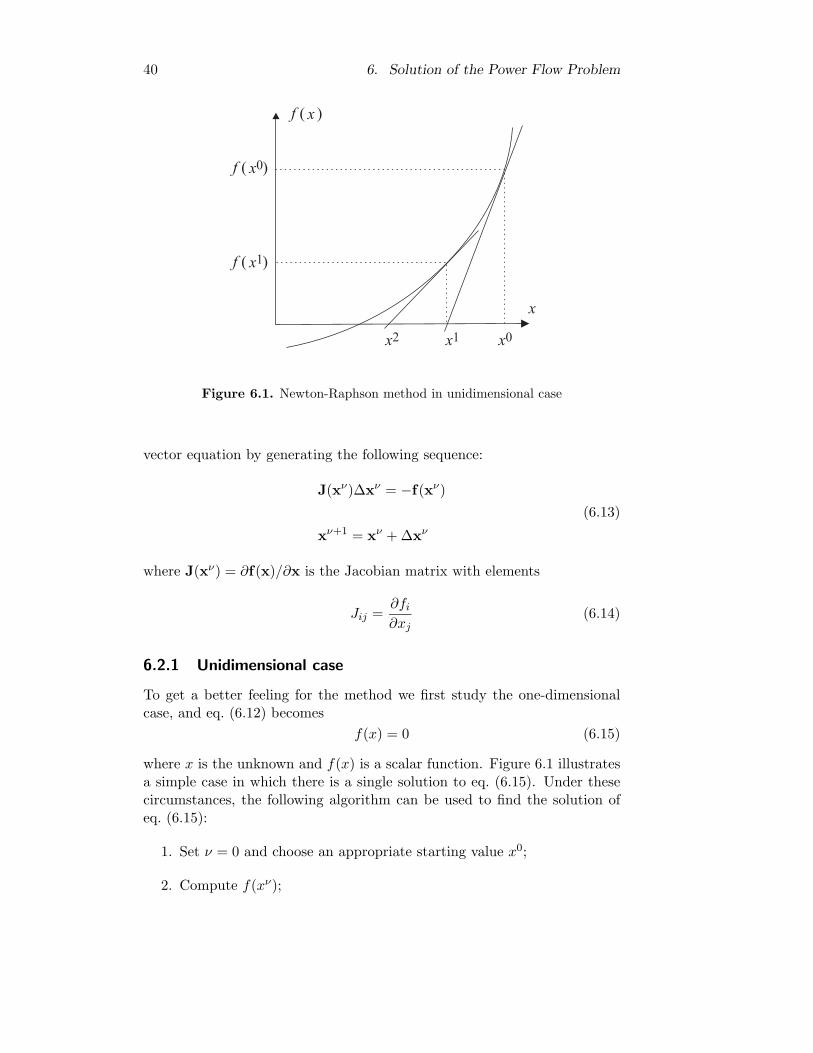
where x is the unknown and f(x) is a scalar function. Figure 6.1 illustratesa simple case in which there is a single solution to eq. (6.15). Under thesecircumstances, the following algorithm can be used to find the solution ofeq. (6.15):
1. Set ν = 0 and choose an appropriate starting value x0;
2. Compute f(xν);
6.2. Newton-Raphson Method 41
0 /2/2 p-p p
V V xk m km/
P,Q
qkm
Qkm
PkmOperation range
x0x1x2
x1f ( )
x0f ( )
x
xf ( )
x0x1x2
x1f ( )
x0f ( )
x
xf ( )
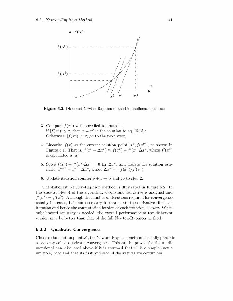
Figure 6.2. Dishonest Newton-Raphson method in unidimensional case
3. Compare f(xν) with specified tolerance ε;if |f(xν)| ≤ ε, then x = xν is the solution to eq. (6.15);Otherwise, |f(xν)| > ε, go to the next step;
4. Linearize f(x) at the current solution point [xν , f(xν)], as shown inFigure 6.1. That is, f(xν + ∆xν) ≈ f(xν) + f ′(xν)∆xν , where f ′(xν)is calculated at xν
5. Solve f(xν) + f ′(xν)∆xν = 0 for ∆xν , and update the solution esti-mate, xν+1 = xν + ∆xν , where ∆xν = −f(xν)/f ′(xν);
6. Update iteration counter ν + 1 → ν and go to step 2.
The dishonest Newton-Raphson method is illustrated in Figure 6.2. Inthis case at Step 4 of the algorithm, a constant derivative is assigned andf ′(xν) = f ′(x0). Although the number of iterations required for convergenceusually increases, it is not necessary to recalculate the derivatives for eachiteration and hence the computation burden at each iteration is lower. Whenonly limited accuracy is needed, the overall performance of the dishonestversion may be better than that of the full Newton-Raphson method.
6.2.2 Quadratic Convergence
Close to the solution point x∗, the Newton-Raphson method normally presentsa property called quadratic convergence. This can be proved for the unidi-mensional case discussed above if it is assumed that x∗ is a simple (not amultiple) root and that its first and second derivatives are continuous.
42 6. Solution of the Power Flow Problem
Hence, f ′(x∗) = 0, and for any x in a certain neighbourhood of x∗,f ′(x) 6= 0. If εν denotes the error at the ν-th iteration, i.e.
εν = x∗ − x(ν) (6.16)
the Taylor expansion about xν yields
f(x∗) = f(x(ν) + εν)
= f(x(ν)) + f ′(x(ν))εν + 1/2f ′′(x)ε2ν (6.17)
= 0
where x ∈ [x(ν), x∗]. Dividing by f ′(x(ν)), this expression can be written as
f(x(ν))
f ′(x(ν))+ εν + 1/2
f ′′(x)
f ′(x(ν))ε2ν = 0 (6.18)
Since,
f(x(ν))
f ′(x(ν))+ εν =
f(x(ν))
f ′(x(ν))+ x∗ − x(ν) = x∗ − x(ν+1) = εν+1 (6.19)
the following relationship between εν and εν+1 results:
εν+1
ε2ν
= −1
2
f ′′(x)
f ′(xν)(6.20)
In the vicinity of the root, i.e. as xν → x∗, x → x∗, and we thus have
|εν+1| =1
2
|f ′′(x∗)||f ′(x∗)| εν
2 (6.21)
From eq. (6.21) it is clear that the convergence is quadratic with the as-sumptions stated above.
6.2.3 Multidimensional Case
Reconsider now the n-dimensional case
f(x) = 0 (6.22)
wheref(x) = (f1(x), f2(x), . . . , fn(x))T (6.23)
andx = (x1, x2, . . . , xn)T (6.24)
Thus f(x) and x are n-dimensional (column) vectors.The Newton-Raphson method applied to to solve eq. (6.22) follows ba-
sically the same steps as those applied to the unidimensional case above,
6.2. Newton-Raphson Method 43
except that in Step 4, the Jacobian matrix J(xν) is used, and the lineariza-tion of f(x) at xν is given by the Taylor expansion
f(xν + ∆xν) ≈ f(xν) + J(xν)∆xν (6.25)
where the Jacobian matrix has the general form
J =∂f
∂x=
∂f1
∂x1
∂f1
∂x2· · · ∂f1
∂xn
∂f2
∂x1
∂f2
∂x2· · · ∂f2
∂xn...
.... . .
...∂fn
∂x1
∂fn
∂x2· · · ∂fn
∂xn
(6.26)
The correction vector ∆x is the solution to
f(xν) + J(xν)∆xν = 0 (6.27)
Note that this is the linearized version of the original problem f(xν +∆xν) =0. The solution of eq. (6.27) involves thus the solution of a system of linearequations, which usually is done by Gauss elimination (LU factorization).
The Newton-Raphson algorithm for the n-dimensional case is thus asfollows:
1. Set ν = 0 and choose an appropriate starting value x0;
2. Compute f(xν);
3. Test convergence:If |fi(x
ν)| ≤ ε for i = 1, 2, . . . , n, then xν is the solutionOtherwise go to 4;
4. Compute the Jacobian matrix J(xν);
5. Update the solution
∆xν = −J−1(xν)f(xν)
(6.28)
xν+1 = xν + ∆xν
6. Update iteration counter ν + 1 → ν and go to step 2.
44 6. Solution of the Power Flow Problem
6.3 Newton-Raphson applied to the Power Flow Equa-
tions
In this section we will now formulate the Newton-Raphson iteration of thepower flow equations. Firstly, the state vector of unknown voltage anglesand magnitudes is ordered such that
x =
(
θU
)
(6.29)
and the nonlinear function f is ordered so that the first components corre-spond to active power and the last ones to reactive power:
f(x) =
(
∆P(x)∆Q(x)
)
=
(
P(x) − P(s)
Q(x) − Q(s)
)
(6.30)
with
f(x) =
P2(x) − P(s)2
...
Pm(x) − P(s)m
−−−−−−Q2(x) − Q
(s)2
...
Qn(x) − Q(s)n
(6.31)
In eq. (6.31) the functions Pk(x) are the active power flows out from bus k
given by eq. (4.11) and the P(s)k are the known active power injections into
bus k from generators and loads, and the functions Qk(x) are the reactive
power flows out from bus k given by eq. (4.12) and Q(s)k are the known
reactive power injections into bus k from generators and loads. The firstm − 1 equations are formulated for PU and PQ buses, and the last n − 1equations can only be formulated for PQ buses. If there are NPU PU busesand NPQ PQ buses, m− 1 = NPU + NPQ and n− 1 = NPQ. The load flowequations can now be written as
f(x) =
(
∆P(x)∆Q(x)
)
= 0 (6.32)
and the functions ∆P(x) and ∆Q(x) are called active and reactive (power)mismatches. The updates to the solutions are determined from the equation
J(xν)
(
∆θν
∆Uν
)
+
(
∆P(xν)∆Q(xν)
)
= 0 (6.33)
6.4. Pθ − QU Decoupling 45
The Jacobian matrix J can be written as
J =
∂∆P
∂θ
∂∆P
∂U
∂∆Q
∂θ
∂∆Q
∂U
(6.34)
which is equal to
J =
∂P(x)
∂θ
∂P(x)
∂U
∂Q(x)
∂θ
∂Q(x)
∂U
(6.35)
or simply
J =
∂P
∂θ
∂P
∂U
∂Q
∂θ
∂Q
∂U
(6.36)
In eq. (6.34) the matrices ∂P/∂θ and ∂Q/∂U are always quadratic, and sois of course J.
6.4 Pθ − QU Decoupling
The ac power flow problem above involves four variables associated witheach network node k:
• Uk, the voltage magnitude
• θk, the voltage angle
• Pk, the net active power (generation – load)
• Qk, the net reactive power (generation – load)
For transmission systems, a strong coupling is normally observed betweenP and θ, as well as between Q and U . This property will in this section beemployed to simplify and speed up the computations. In the next sectionwe will derive a linear approximation called dc power flow (or dc load flow).This linear model relates the active power P to the bus voltage angle θ.
Let us consider a π-model of a transmission line, where the series resis-tance and the shunt admittance both are neglected and put to zero. In thiscase, the active and reactive power flows are given by the following simplifiedexpressions of eqs. (3.3) and (3.4)
Pkm =UkUm sin θkm
xkm(6.37)
46 6. Solution of the Power Flow Problem
Qkm =U2
k − UkUm cos θkm
xkm(6.38)
where xkm is the series reactance of the line.The sensitivities between power flows Pkm and Qkm and the state vari-
ables U and θ are for this approximation given by
∂Pkm
∂θk=
UkUm cos θkm
xkm
∂Pkm
∂Uk=
Um sin θkm
xkm(6.39)
∂Qkm
∂θk=
UkUm sin θkm
xkm
∂Qkm
∂Uk=
2Uk − Um cos θkm
xkm(6.40)
When θkm = 0, perfect decoupling conditions are observed, i.e.
∂Pkm
∂θk=
UkUm
xkm
∂Pkm
∂Uk= 0 (6.41)
∂Qkm
∂θk= 0
∂Qkm
∂Uk=
2Uk − Um
xkm(6.42)
As illustrated in Figure 6.3, in the usual range of operations (relatively smallvoltage angles), a strong coupling between active power and voltage angle aswell as between reactive power and voltage magnitudes exists, while a muchweaker coupling between reactive power and voltage angle, and betweenvoltage magnitude and active power exists. Notice, however, that for largerangles this is no longer true. In the neighbourhood of θkm = 90, there isstrong coupling between P and U as well as between Q and θ.
Example 6.1. A 750 kV transmission line has 0.0175 p.u. series reactance(the series resistance and the shunt admittance are ignored in this example).The terminal bus voltage magnitudes are 0.984 and 0.962 p.u. and the angledifference is 10. Calculate the sensitivities of the active and reactive powerflows with respect to voltage magnitude and phase angle.
Solution The four sensitivities are calculated by using eqs. (6.39) and(6.40):
∂Pkm
∂θk=
UkUm cos θkm
xkm=
0.984 · 0.962 cos 10
0.0175= 54.1
∂Pkm
∂Uk=
Um sin θkm
xkm=
0.962 sin 10
0.0175= 9.5
∂Qkm
∂θk=
UkUm sin θkm
xkm=
0.984 · 0.962 sin 10
0.0175= 9.4
∂Qkm
∂Uk=
2Uk − Um cos θkm
xkm=
2 · 0.984 − 0.962 cos 10
0.0175= 58.3
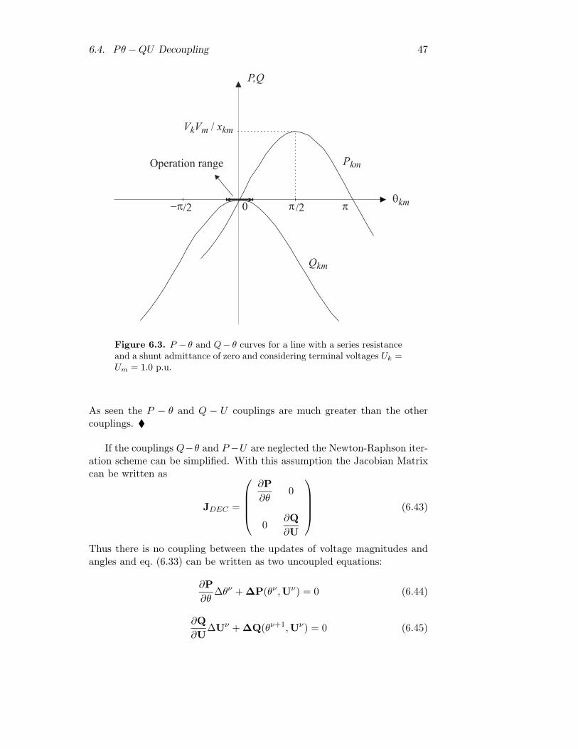
6.4. Pθ − QU Decoupling 47
0 /2/2 p-p p
V V xk m km/
P,Q
qkm
Qkm
PkmOperation range
x0x1x2
x1f ( )
x0f ( )
x
xf ( )
x0x1x2
x1f ( )
x0f ( )
x
xf ( )
Figure 6.3. P − θ and Q− θ curves for a line with a series resistanceand a shunt admittance of zero and considering terminal voltages Uk =Um = 1.0 p.u.
As seen the P − θ and Q − U couplings are much greater than the othercouplings.
If the couplings Q−θ and P −U are neglected the Newton-Raphson iter-ation scheme can be simplified. With this assumption the Jacobian Matrixcan be written as
JDEC =
∂P
∂θ0
0∂Q
∂U
(6.43)
Thus there is no coupling between the updates of voltage magnitudes andangles and eq. (6.33) can be written as two uncoupled equations:
∂P
∂θ∆θν + ∆P(θν ,Uν) = 0 (6.44)
∂Q
∂U∆Uν + ∆Q(θν+1,Uν) = 0 (6.45)
48 6. Solution of the Power Flow Problem
In this formulation two systems of linear equations have to be solved insteadof one system. Of course, the total number of equations to be solved isthe same, but since the needed number of operations to solve a system oflinear equations increases more than linearly with the dimension, it takes lessoperations to solve eqs. (6.44) and (6.45) than eq. (6.33) with the completeJacobian matrix, J. It should be noted that if the iterations of eqs. (6.44) and(6.45) converge, it converges to a correct solution of the load flow equations.No approximations have been introduced in the functions P(x) or Q(x),only in the way we calculate the updates. The convergence of the decoupledscheme is somewhat slower than the full scheme, but often the faster solutiontime for the updates compensates for slower convergence, giving as fasteroverall solution time. For not too heavily loaded systems a faster overallsolution time is almost always obtained. The two equations (6.44) and (6.45)are solved sequentially, and then the updated unknowns of the first equation,eq. (6.44), can be used to calculate the mismatches of the second system ofequations, eq. (6.45), resulting in an increased speed of convergence.
A number of approximations can be made to calculate the matrix ele-ments of the the two sub-matrices of the Jacobian in eqs. (6.44) and (6.45).This will only influence the speed of convergence of the solution. If themethod converges to a solution, this is the correct solution as long as theaccurate expression for ∆P and ∆Q are used.
If approximations regarding the active and reactive power mismatchesare used, the solution can be even faster, but then only an approximativesolution will be obtained. This is further elaborated in the next section.
6.5 Approximative Solutions of the Power Flow Prob-
lem
In the previous section the exact expressions of the power flow equationswere used. However, since the power flow equations are solved frequentlyin the operation and planning of electric power systems there is a needthat the equations can be solved fast, and for this purpose the approxima-tions introduced in this chapter have proved to be of great value. Oftenthe approximations described here are used together with exact methods.Approximative methods could be used to identify the most critical cases,which are then further analysed with the full models. The fast, approxima-tive methods can also used to provide good initial guesses for a completesolution of the equations.
6.5.1 Linearization
In this subsection the linearized dc power flow equations will be derived.
6.5. Approximative Solutions of the Power Flow Problem 49
Transmission Line
Consider again expressions for the active power flows (Pkm and Pmk) in atransmission line:
Pkm = U2kgkm − UkUmgkm cos θkm − UkUmbkm sin θkm (6.46)
Pmk = U2mgkm − UkUmgkm cos θkm + UkUmbkm sin θkm (6.47)
These equations can be used to determine the real power losses in atransmission line
Pkm + Pmk = gkm(U2k + U2
m − 2UkUm cos θkm) (6.48)
If the terms corresponding to the active power losses are ignored in eqs.(6.46) and (6.47), the result is
Pkm = −Pmk = −UkUmbkm sin θkm (6.49)
The following additional approximations are often valid, particularly duringlight load conditions
Uk ≈ Um ≈ 1 p.u. (6.50)
sin θkm ≈ θkm (6.51)
And sincebkm = −1/xkm (6.52)
we can simplify the expression for the active power flow Pkm to
Pkm = θkm/xkm =θk − θm
xkm(6.53)
This equation is analogous to Ohm’s law applied to a resistor carrying adc current:
• Pkm is the dc current;
• θk and θm are the dc voltages at the resistor terminals;
• xkm is the resistance.
This is illustrated in Figure 6.4.
Series Capacitor
For a given voltage angle spread, the active power flow in a transmission linedecreases with the line reactance (and series reactance normally increaseswith line length). Series compensation aims at reducing the effective electriclength of the line: a series capacitor connected in series with the line. If, forexample, a 40% compensation corresponds to a capacitor with a reactance
50 6. Solution of the Power Flow Problem
k mrkm + jxkm
jb jbkm km
sh sh (a)
k
(b)
mxkm
Pkm mk= (q - q ) xkm
PU PQ
PQUq
PU
1 2 3
45
Figure 6.4. Transmission line. (a) Equivalent π-model. (b) DC powerflow model.
of 40% of the original line reactance, but with opposite sign, the resultingreactance of the compensated line becomes 60% of the original value. Thus
xcompkm = xkm − xsc (6.54)
with obvious notation. In the dc power flow model the series capacitorcan thus be regarded as a negative resistance inserted in series with theequivalent line resistance.
In-Phase Transformer
The active power flows, Pkm and Pmk, in an in-phase transformer are givenby eq. (3.10)
Pkm = (akmUk)2gkm − akmUkUmgkm cos θkm − akmUkUmbkm sin θkm (6.55)
Neglecting the terms associated with losses and introducing the same ap-proximations used for transmission lines yields
Pkm =θkm
xkm/akm(6.56)
where further approximating akm ≈ 1, i.e. the transformer tap ratio is closeto the relation between the nominal voltages of the two sides, yields the
6.5. Approximative Solutions of the Power Flow Problem 51
k
k
lm
k lrml + jxml
jxkm
m
jb jbml ml
sh sh (a)
(b)
(a)
(b)
k m
m
1:akm jxkm
Pkm mk= (q - q ) xkm
xkm akm
Pkm mk= (q - q ) (xkm akm)
Figure 6.5. In-phase transformer. (a) Transformer comprising idealtransformer and series reactance. (b) DC power flow model.
same expression as for transmission lines
Pkm =θkm
xkm(6.57)
This is illustrated in Figure 6.5.
Phase Shifter
Let us consider again the expression for the active power flow Pkm in a phase-shifting transformer of the type represented in Figure 2.6 with akm = 1(eq. (3.14)):
Pkm = U2kgkm − UkUmgkm cos(θkm + ϕkm) − UkUmbkm sin(θkm + ϕkm)
As with transmission lines and in-phase transformers, if the terms as-sociated with active power losses are ignored and Uk = Um = 1 p.u. andbkm = −x−1
km, the result is
Pkm =sin(θkm + ϕkm)
xkm(6.58)
and if (θkm + ϕkm) ≪ π/2, then linear approximation can be used, giving
Pkm =(θkm + ϕkm)
xkm(6.59)
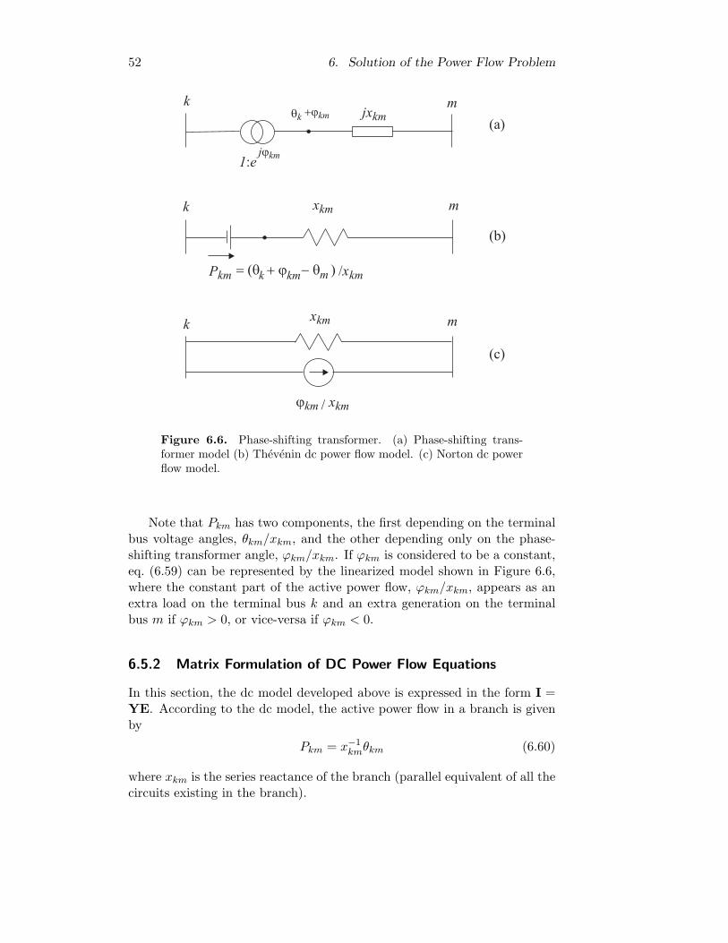
52 6. Solution of the Power Flow Problem
k
k
k
m
m
m
1:ejjkm
jxkm
xkm
xkm
qk +jkm
jkm xkm/
(a)
(b)
(c)
Pkm km mk= (q + j - q ) /xkm
Figure 6.6. Phase-shifting transformer. (a) Phase-shifting trans-former model (b) Thevenin dc power flow model. (c) Norton dc powerflow model.
Note that Pkm has two components, the first depending on the terminalbus voltage angles, θkm/xkm, and the other depending only on the phase-shifting transformer angle, ϕkm/xkm. If ϕkm is considered to be a constant,eq. (6.59) can be represented by the linearized model shown in Figure 6.6,where the constant part of the active power flow, ϕkm/xkm, appears as anextra load on the terminal bus k and an extra generation on the terminalbus m if ϕkm > 0, or vice-versa if ϕkm < 0.
6.5.2 Matrix Formulation of DC Power Flow Equations
In this section, the dc model developed above is expressed in the form I =YE. According to the dc model, the active power flow in a branch is givenby
Pkm = x−1kmθkm (6.60)
where xkm is the series reactance of the branch (parallel equivalent of all thecircuits existing in the branch).
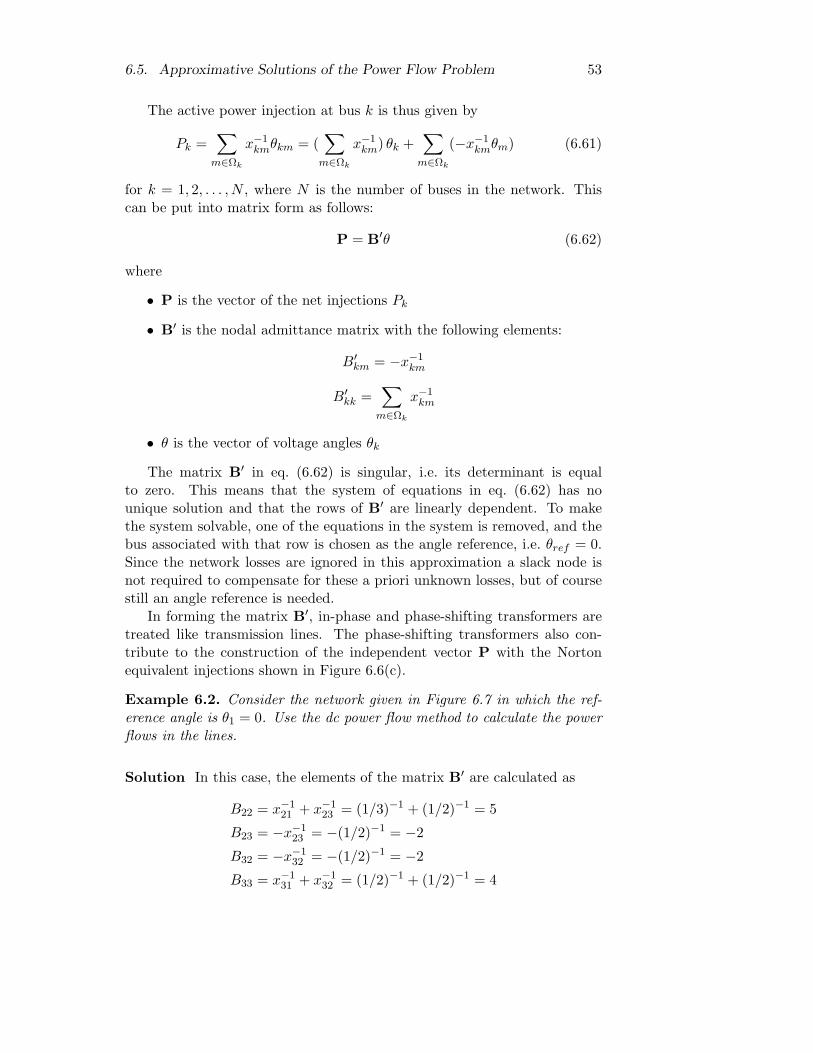
6.5. Approximative Solutions of the Power Flow Problem 53
The active power injection at bus k is thus given by
Pk =∑
m∈Ωk
x−1kmθkm = (
∑
m∈Ωk
x−1km) θk +
∑
m∈Ωk
(−x−1kmθm) (6.61)
for k = 1, 2, . . . , N , where N is the number of buses in the network. Thiscan be put into matrix form as follows:
P = B′θ (6.62)
where
• P is the vector of the net injections Pk
• B′ is the nodal admittance matrix with the following elements:
B′km = −x−1
km
B′kk =
∑
m∈Ωk
x−1km
• θ is the vector of voltage angles θk
The matrix B′ in eq. (6.62) is singular, i.e. its determinant is equalto zero. This means that the system of equations in eq. (6.62) has nounique solution and that the rows of B′ are linearly dependent. To makethe system solvable, one of the equations in the system is removed, and thebus associated with that row is chosen as the angle reference, i.e. θref = 0.Since the network losses are ignored in this approximation a slack node isnot required to compensate for these a priori unknown losses, but of coursestill an angle reference is needed.
In forming the matrix B′, in-phase and phase-shifting transformers aretreated like transmission lines. The phase-shifting transformers also con-tribute to the construction of the independent vector P with the Nortonequivalent injections shown in Figure 6.6(c).
Example 6.2. Consider the network given in Figure 6.7 in which the ref-erence angle is θ1 = 0. Use the dc power flow method to calculate the powerflows in the lines.
Solution In this case, the elements of the matrix B′ are calculated as
B22 = x−121 + x−1
23 = (1/3)−1 + (1/2)−1 = 5
B23 = −x−123 = −(1/2)−1 = −2
B32 = −x−132 = −(1/2)−1 = −2
B33 = x−131 + x−1
32 = (1/2)−1 + (1/2)−1 = 4
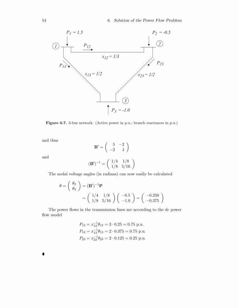
54 6. Solution of the Power Flow Problem
P1
P13
P12
P23
P2
P3
= 1.5 = -0.5
= -1.0
1
3
2
x 1/312 =
x 1/213 = x 1/223 =
Figure 6.7. 3-bus network. (Active power in p.u.; branch reactances in p.u.)
and thus
B′ =
(
5 −2−2 4
)
and
(B′)−1 =
(
1/4 1/81/8 5/16
)
The nodal voltage angles (in radians) can now easily be calculated
θ =
(
θ2
θ3
)
= (B′)−1P
=
(
1/4 1/81/8 5/16
)(
−0.5−1.0
)
=
(
−0.250−0.375
)
The power flows in the transmission lines are according to the dc powerflow model
P12 = x−112 θ12 = 3 · 0.25 = 0.75 p.u.
P13 = x−113 θ13 = 2 · 0.375 = 0.75 p.u.
P23 = x−123 θ23 = 2 · 0.125 = 0.25 p.u.

6.5. Approximative Solutions of the Power Flow Problem 55
6.5.3 DC Power Flow Model
The linearized model P = B′θ can be interpreted as the model for a net-work of resistors fed by dc current sources where P is the vector of nodalcurrent injections, θ is the nodal vector of dc voltages, and B′ is the nodalconductance matrix, as illustrated in Figure 6.8.
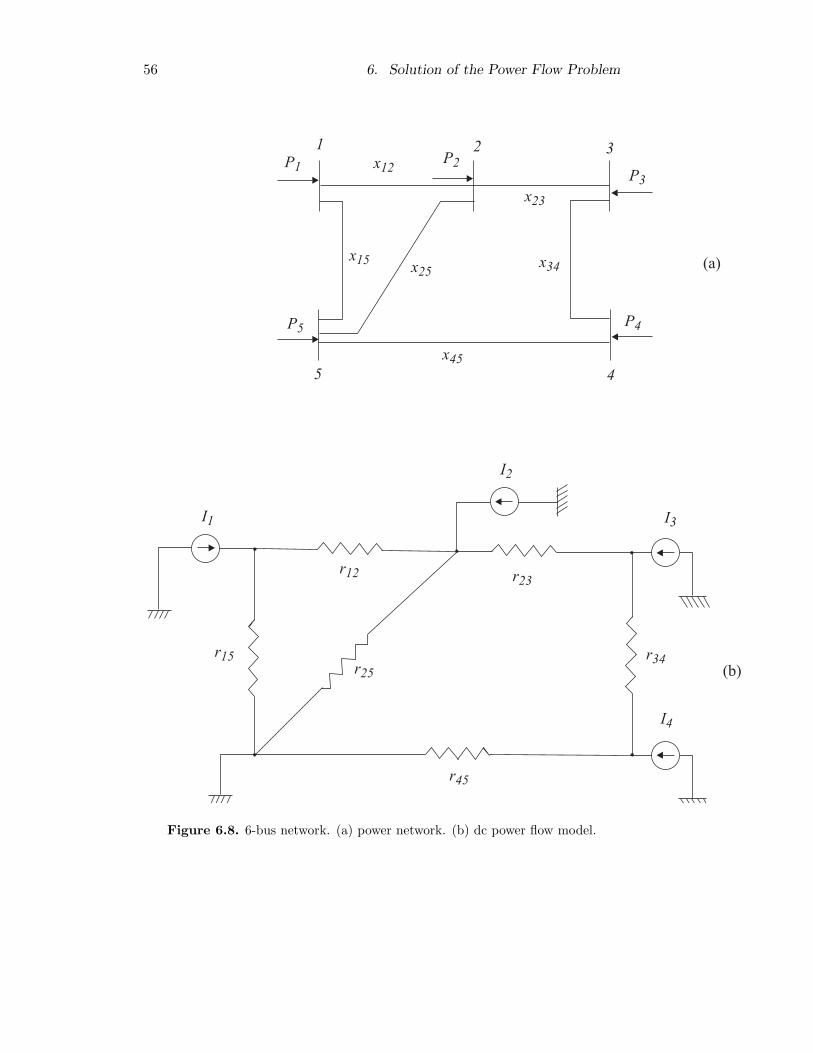
56 6. Solution of the Power Flow Problem
1 2 3
45
P1P2
P3
P4P5
x12
x23
x34
x45
x25
x15
I1 I3
I2
I4
r15
r12
r25
r45
r23
r34
(a)
(b)
Figure 6.8. 6-bus network. (a) power network. (b) dc power flow model.
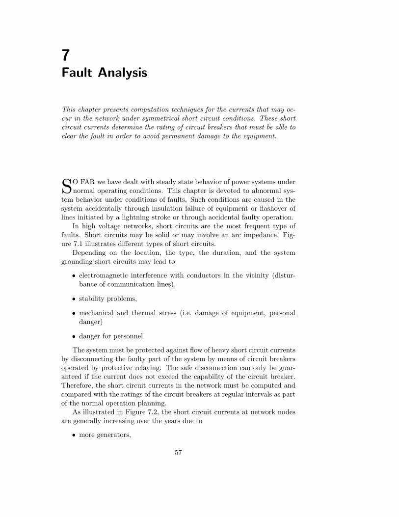
7Fault Analysis
This chapter presents computation techniques for the currents that may oc-cur in the network under symmetrical short circuit conditions. These shortcircuit currents determine the rating of circuit breakers that must be able toclear the fault in order to avoid permanent damage to the equipment.
SO FAR we have dealt with steady state behavior of power systems undernormal operating conditions. This chapter is devoted to abnormal sys-
tem behavior under conditions of faults. Such conditions are caused in thesystem accidentally through insulation failure of equipment or flashover oflines initiated by a lightning stroke or through accidental faulty operation.
In high voltage networks, short circuits are the most frequent type offaults. Short circuits may be solid or may involve an arc impedance. Fig-ure 7.1 illustrates different types of short circuits.
Depending on the location, the type, the duration, and the systemgrounding short circuits may lead to
• electromagnetic interference with conductors in the vicinity (distur-bance of communication lines),
• stability problems,
• mechanical and thermal stress (i.e. damage of equipment, personaldanger)
• danger for personnel
The system must be protected against flow of heavy short circuit currentsby disconnecting the faulty part of the system by means of circuit breakersoperated by protective relaying. The safe disconnection can only be guar-anteed if the current does not exceed the capability of the circuit breaker.Therefore, the short circuit currents in the network must be computed andcompared with the ratings of the circuit breakers at regular intervals as partof the normal operation planning.
As illustrated in Figure 7.2, the short circuit currents at network nodesare generally increasing over the years due to
• more generators,
57
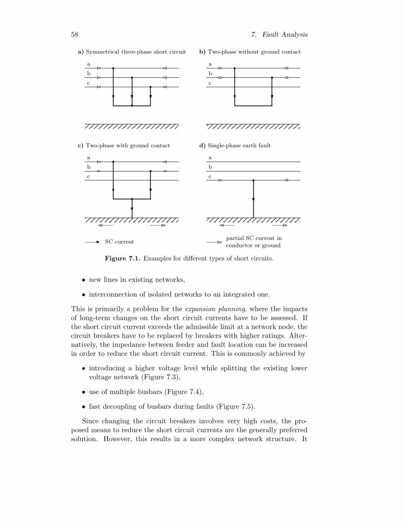
58 7. Fault Analysis
a) Symmetrical three-phase short circuit b) Two-phase without ground contact
c) Two-phase with ground contact d) Single-phase earth fault
a
a a
a
b
b b
b
c
c c
c
SC currentpartial SC current inconductor or ground
Figure 7.1. Examples for different types of short circuits.
• new lines in existing networks,
• interconnection of isolated networks to an integrated one.
This is primarily a problem for the expansion planning, where the impactsof long-term changes on the short circuit currents have to be assessed. Ifthe short circuit current exceeds the admissible limit at a network node, thecircuit breakers have to be replaced by breakers with higher ratings. Alter-natively, the impedance between feeder and fault location can be increasedin order to reduce the short circuit current. This is commonly achieved by
• introducing a higher voltage level while splitting the existing lowervoltage network (Figure 7.3),
• use of multiple busbars (Figure 7.4),
• fast decoupling of busbars during faults (Figure 7.5).
Since changing the circuit breakers involves very high costs, the pro-posed means to reduce the short circuit currents are the generally preferredsolution. However, this results in a more complex network structure. It
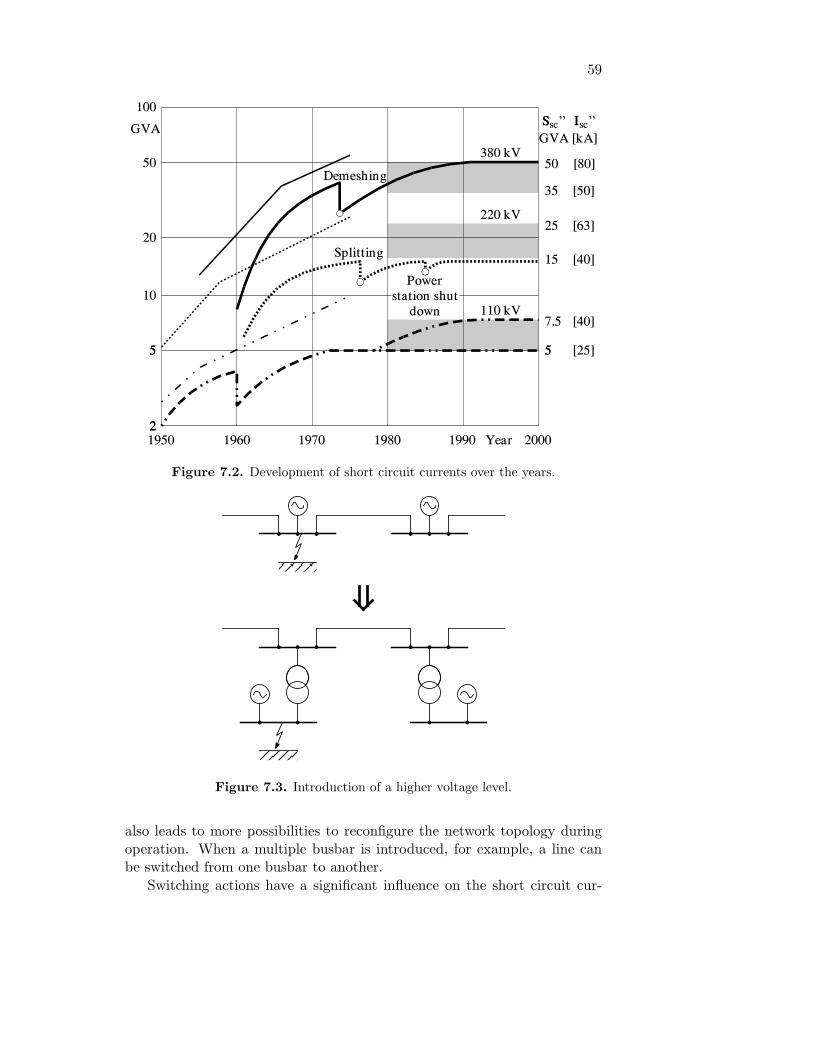
59
Figure 7.2. Development of short circuit currents over the years.
Figure 7.3. Introduction of a higher voltage level.
also leads to more possibilities to reconfigure the network topology duringoperation. When a multiple busbar is introduced, for example, a line canbe switched from one busbar to another.
Switching actions have a significant influence on the short circuit cur-
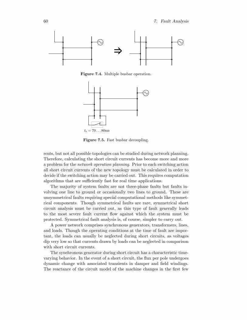
60 7. Fault Analysis
Figure 7.4. Multiple busbar operation.
ts = 70 . . . 80ms
Figure 7.5. Fast busbar decoupling.
rents, but not all possible topologies can be studied during network planning.Therefore, calculating the short circuit currents has become more and morea problem for the network operation planning. Prior to each switching actionall short circuit currents of the new topology must be calculated in order todecide if the switching action may be carried out. This requires computationalgorithms that are sufficiently fast for real time applications.
The majority of system faults are not three-phase faults but faults in-volving one line to ground or occasionally two lines to ground. These areunsymmetrical faults requiring special computational methods like symmet-rical components. Though symmetrical faults are rare, symmetrical shortcircuit analysis must be carried out, as this type of fault generally leadsto the most severe fault current flow against which the system must beprotected. Symmetrical fault analysis is, of course, simpler to carry out.
A power network comprises synchronous generators, transformers, lines,and loads. Though the operating conditions at the time of fault are impor-tant, the loads can usually be neglected during short circuits, as voltagesdip very low so that currents drawn by loads can be neglected in comparisonwith short circuit currents.
The synchronous generator during short circuit has a characteristic time-varying behavior. In the event of a short circuit, the flux per pole undergoesdynamic change with associated transients in damper and field windings.The reactance of the circuit model of the machine changes in the first few
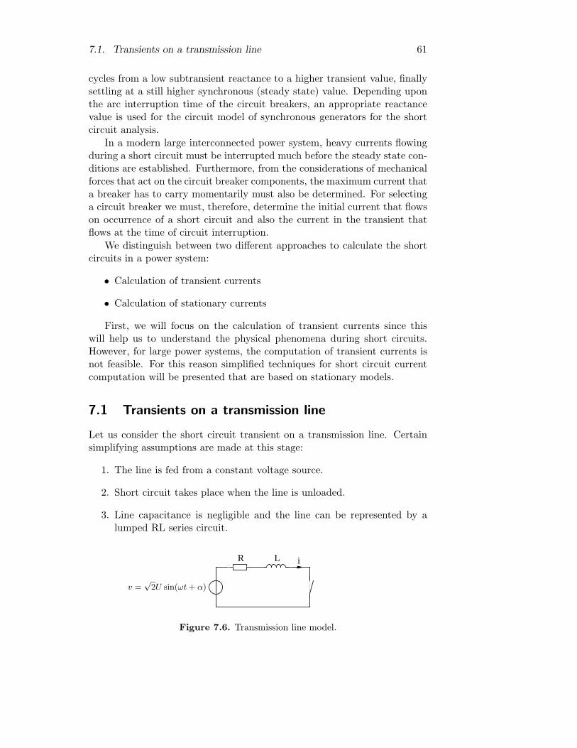
7.1. Transients on a transmission line 61
cycles from a low subtransient reactance to a higher transient value, finallysettling at a still higher synchronous (steady state) value. Depending uponthe arc interruption time of the circuit breakers, an appropriate reactancevalue is used for the circuit model of synchronous generators for the shortcircuit analysis.
In a modern large interconnected power system, heavy currents flowingduring a short circuit must be interrupted much before the steady state con-ditions are established. Furthermore, from the considerations of mechanicalforces that act on the circuit breaker components, the maximum current thata breaker has to carry momentarily must also be determined. For selectinga circuit breaker we must, therefore, determine the initial current that flowson occurrence of a short circuit and also the current in the transient thatflows at the time of circuit interruption.
We distinguish between two different approaches to calculate the shortcircuits in a power system:
• Calculation of transient currents
• Calculation of stationary currents
First, we will focus on the calculation of transient currents since thiswill help us to understand the physical phenomena during short circuits.However, for large power systems, the computation of transient currents isnot feasible. For this reason simplified techniques for short circuit currentcomputation will be presented that are based on stationary models.
7.1 Transients on a transmission line
Let us consider the short circuit transient on a transmission line. Certainsimplifying assumptions are made at this stage:
1. The line is fed from a constant voltage source.
2. Short circuit takes place when the line is unloaded.
3. Line capacitance is negligible and the line can be represented by alumped RL series circuit.
R L i
v =√
2U sin(ωt + α)
Figure 7.6. Transmission line model.
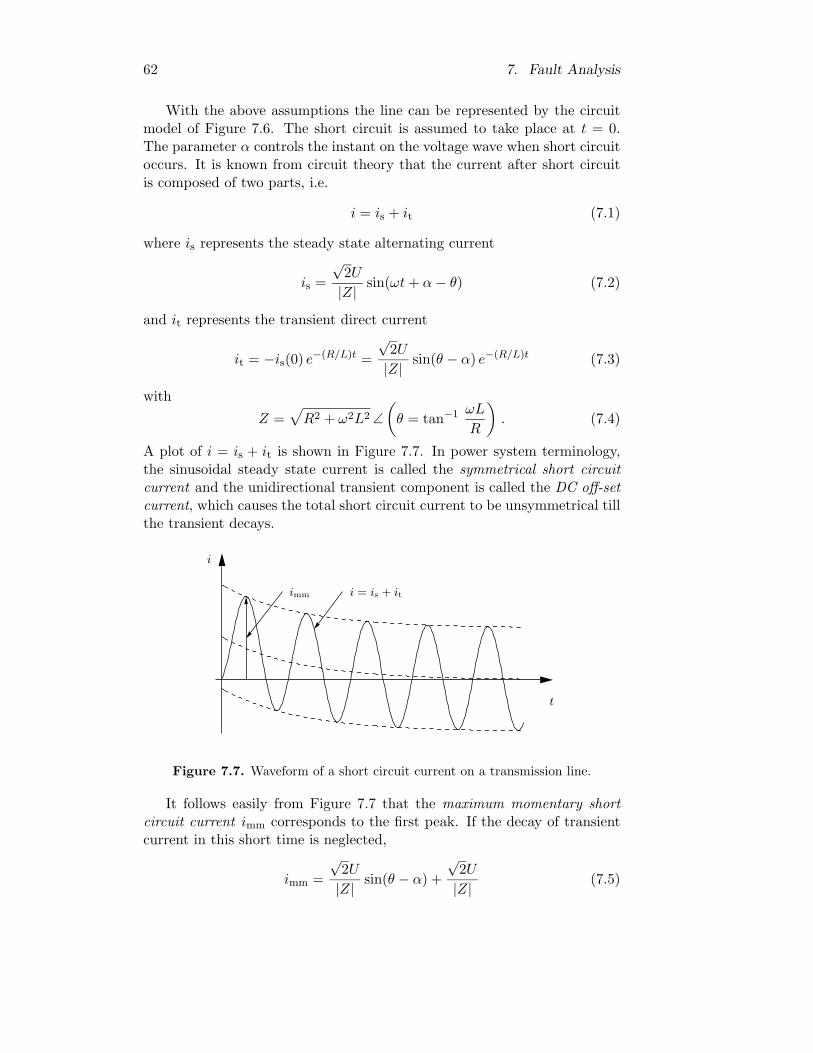
62 7. Fault Analysis
With the above assumptions the line can be represented by the circuitmodel of Figure 7.6. The short circuit is assumed to take place at t = 0.The parameter α controls the instant on the voltage wave when short circuitoccurs. It is known from circuit theory that the current after short circuitis composed of two parts, i.e.
i = is + it (7.1)
where is represents the steady state alternating current
is =
√2U
|Z| sin(ωt + α − θ) (7.2)
and it represents the transient direct current
it = −is(0) e−(R/L)t =
√2U
|Z| sin(θ − α) e−(R/L)t (7.3)
with
Z =√
R2 + ω2L2 ∠
(
θ = tan−1 ωL
R
)
. (7.4)
A plot of i = is + it is shown in Figure 7.7. In power system terminology,the sinusoidal steady state current is called the symmetrical short circuitcurrent and the unidirectional transient component is called the DC off-setcurrent, which causes the total short circuit current to be unsymmetrical tillthe transient decays.
imm
i
t
i = is + it
Figure 7.7. Waveform of a short circuit current on a transmission line.
It follows easily from Figure 7.7 that the maximum momentary shortcircuit current imm corresponds to the first peak. If the decay of transientcurrent in this short time is neglected,
imm =
√2U
|Z| sin(θ − α) +
√2U
|Z| (7.5)
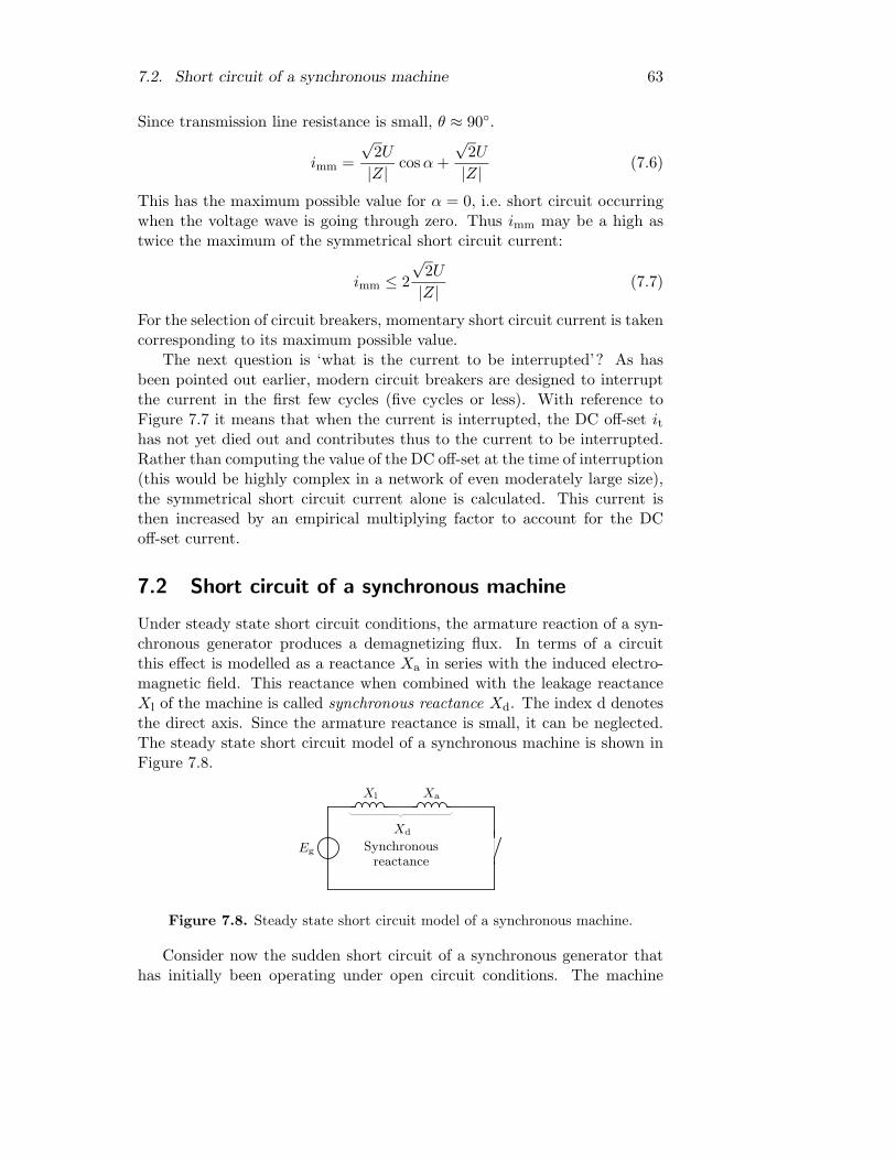
7.2. Short circuit of a synchronous machine 63
Since transmission line resistance is small, θ ≈ 90.
imm =
√2U
|Z| cos α +
√2U
|Z| (7.6)
This has the maximum possible value for α = 0, i.e. short circuit occurringwhen the voltage wave is going through zero. Thus imm may be a high astwice the maximum of the symmetrical short circuit current:
imm ≤ 2
√2U
|Z| (7.7)
For the selection of circuit breakers, momentary short circuit current is takencorresponding to its maximum possible value.
The next question is ‘what is the current to be interrupted’? As hasbeen pointed out earlier, modern circuit breakers are designed to interruptthe current in the first few cycles (five cycles or less). With reference toFigure 7.7 it means that when the current is interrupted, the DC off-set ithas not yet died out and contributes thus to the current to be interrupted.Rather than computing the value of the DC off-set at the time of interruption(this would be highly complex in a network of even moderately large size),the symmetrical short circuit current alone is calculated. This current isthen increased by an empirical multiplying factor to account for the DCoff-set current.
7.2 Short circuit of a synchronous machine
Under steady state short circuit conditions, the armature reaction of a syn-chronous generator produces a demagnetizing flux. In terms of a circuitthis effect is modelled as a reactance Xa in series with the induced electro-magnetic field. This reactance when combined with the leakage reactanceXl of the machine is called synchronous reactance Xd. The index d denotesthe direct axis. Since the armature reactance is small, it can be neglected.The steady state short circuit model of a synchronous machine is shown inFigure 7.8.
Eg
Xl Xa
Xd
Synchronousreactance
Figure 7.8. Steady state short circuit model of a synchronous machine.
Consider now the sudden short circuit of a synchronous generator thathas initially been operating under open circuit conditions. The machine
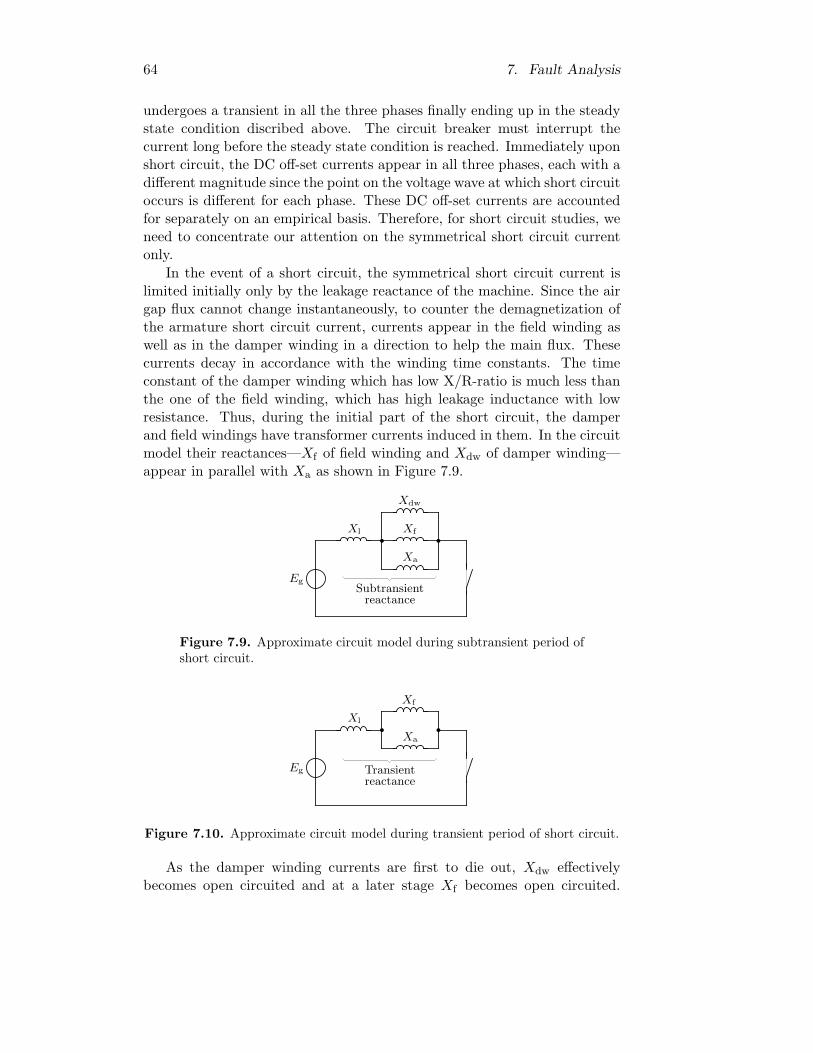
64 7. Fault Analysis
undergoes a transient in all the three phases finally ending up in the steadystate condition discribed above. The circuit breaker must interrupt thecurrent long before the steady state condition is reached. Immediately uponshort circuit, the DC off-set currents appear in all three phases, each with adifferent magnitude since the point on the voltage wave at which short circuitoccurs is different for each phase. These DC off-set currents are accountedfor separately on an empirical basis. Therefore, for short circuit studies, weneed to concentrate our attention on the symmetrical short circuit currentonly.
In the event of a short circuit, the symmetrical short circuit current islimited initially only by the leakage reactance of the machine. Since the airgap flux cannot change instantaneously, to counter the demagnetization ofthe armature short circuit current, currents appear in the field winding aswell as in the damper winding in a direction to help the main flux. Thesecurrents decay in accordance with the winding time constants. The timeconstant of the damper winding which has low X/R-ratio is much less thanthe one of the field winding, which has high leakage inductance with lowresistance. Thus, during the initial part of the short circuit, the damperand field windings have transformer currents induced in them. In the circuitmodel their reactances—Xf of field winding and Xdw of damper winding—appear in parallel with Xa as shown in Figure 7.9.
Eg
Xl
Xa
Xdw
Xf
Subtransientreactance
Figure 7.9. Approximate circuit model during subtransient period ofshort circuit.
Eg
Xl
Xa
Xf
Transientreactance
Figure 7.10. Approximate circuit model during transient period of short circuit.
As the damper winding currents are first to die out, Xdw effectivelybecomes open circuited and at a later stage Xf becomes open circuited.
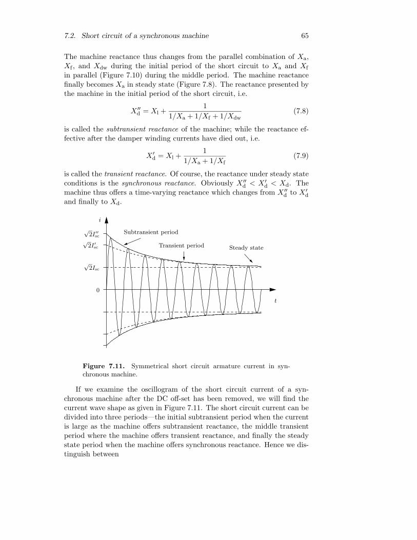
7.2. Short circuit of a synchronous machine 65
The machine reactance thus changes from the parallel combination of Xa,Xf , and Xdw during the initial period of the short circuit to Xa and Xf
in parallel (Figure 7.10) during the middle period. The machine reactancefinally becomes Xa in steady state (Figure 7.8). The reactance presented bythe machine in the initial period of the short circuit, i.e.
X ′′d = Xl +
1
1/Xa + 1/Xf + 1/Xdw(7.8)
is called the subtransient reactance of the machine; while the reactance ef-fective after the damper winding currents have died out, i.e.
X ′d = Xl +
1
1/Xa + 1/Xf(7.9)
is called the transient reactance. Of course, the reactance under steady stateconditions is the synchronous reactance. Obviously X ′′
d < X ′d < Xd. The
machine thus offers a time-varying reactance which changes from X ′′d to X ′
d
and finally to Xd.
i
t
√2I ′′
sc
√2I ′
sc
√2Isc
0
Subtransient period
Transient period Steady state
Figure 7.11. Symmetrical short circuit armature current in syn-chronous machine.
If we examine the oscillogram of the short circuit current of a syn-chronous machine after the DC off-set has been removed, we will find thecurrent wave shape as given in Figure 7.11. The short circuit current can bedivided into three periods—the initial subtransient period when the currentis large as the machine offers subtransient reactance, the middle transientperiod where the machine offers transient reactance, and finally the steadystate period when the machine offers synchronous reactance. Hence we dis-tinguish between
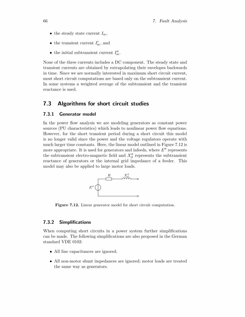
66 7. Fault Analysis
• the steady state current Isc,
• the transient current I ′sc, and
• the initial subtransient current I ′′sc.
None of the three currents includes a DC component. The steady state andtransient currents are obtained by extrapolating their envelopes backwardsin time. Since we are normally interested in maximum short circuit current,most short circuit computations are based only on the subtransient current.In some systems a weighted average of the subtransient and the transientreactance is used.
7.3 Algorithms for short circuit studies
7.3.1 Generator model
In the power flow analysis we are modeling generators as constant powersources (PU characteristics) which leads to nonlinear power flow equations.However, for the short transient period during a short circuit this modelis no longer valid since the power and the voltage regulators operate withmuch larger time constants. Here, the linear model outlined in Figure 7.12 ismore appropriate. It is used for generators and infeeds, where E′′ representsthe subtransient electro-magnetic field and X ′′
d represents the subtransientreactance of generators or the internal grid impedance of a feeder. Thismodel may also be applied to large motor loads.
E′′
X ′′
dR
Figure 7.12. Linear generator model for short circuit computation.
7.3.2 Simplifications
When computing short circuits in a power system further simplificationscan be made. The following simplifications are also proposed in the Germanstandard VDE 0102:
• All line capacitances are ignored.
• All non-motor shunt impedances are ignored; motor loads are treatedthe same way as generators.
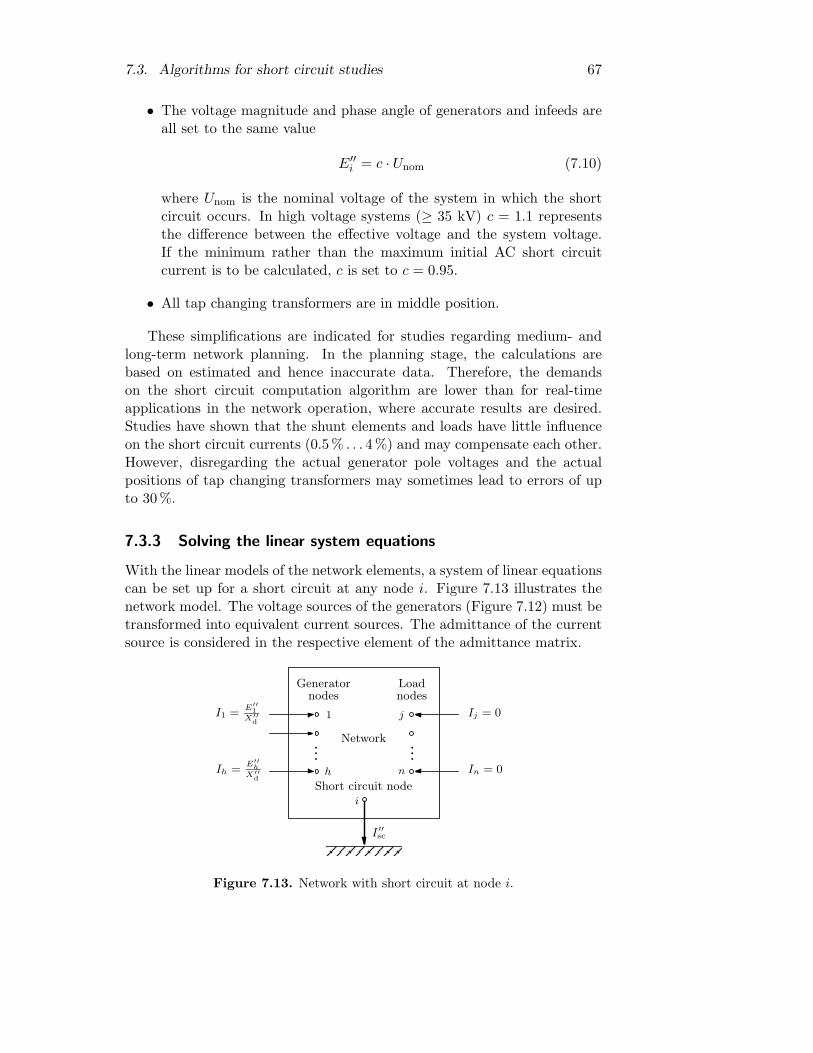
7.3. Algorithms for short circuit studies 67
• The voltage magnitude and phase angle of generators and infeeds areall set to the same value
E′′i = c · Unom (7.10)
where Unom is the nominal voltage of the system in which the shortcircuit occurs. In high voltage systems (≥ 35 kV) c = 1.1 representsthe difference between the effective voltage and the system voltage.If the minimum rather than the maximum initial AC short circuitcurrent is to be calculated, c is set to c = 0.95.
• All tap changing transformers are in middle position.
These simplifications are indicated for studies regarding medium- andlong-term network planning. In the planning stage, the calculations arebased on estimated and hence inaccurate data. Therefore, the demandson the short circuit computation algorithm are lower than for real-timeapplications in the network operation, where accurate results are desired.Studies have shown that the shunt elements and loads have little influenceon the short circuit currents (0.5 % . . . 4 %) and may compensate each other.However, disregarding the actual generator pole voltages and the actualpositions of tap changing transformers may sometimes lead to errors of upto 30 %.
7.3.3 Solving the linear system equations
With the linear models of the network elements, a system of linear equationscan be set up for a short circuit at any node i. Figure 7.13 illustrates thenetwork model. The voltage sources of the generators (Figure 7.12) must betransformed into equivalent current sources. The admittance of the currentsource is considered in the respective element of the admittance matrix.
I1 =E′′
1
X′′
d
Ih =E′′
h
X′′
d
Ij = 0
In = 0
I ′′
sc
1
h
j
n
i
Generatornodes
Loadnodes
Short circuit node
Network
Figure 7.13. Network with short circuit at node i.
68 7. Fault Analysis
In order to calculate the short circuit current I ′′sc at node i the equation
Y · U = I (7.11)
must be solved, where
• Y is the nodal admittance matrix
• U is the nodal voltage vector
U =
Uj if j 6= i
0 if j = i(7.12)
• I is the vector of injection currents
I =
Ej
X ′′dj
for generator nodes j 6= i
0 for load nodes j 6= i
−I ′′sc for short circuit node without generation j = i
−I ′′sc +Ej
X ′′dj
for short circuit node with generation j = i
(7.13)
All elements Uj of vector U are unknown variables with the exception ofvoltage Ui = 0 at the short circuit node i. On the contrary, all elementsof vector I are known except for the current Ii at the short circuit node i.To solve the system of equations (7.11), the ith row and the ith column areremoved. The remaining admittance matrix is then factorized into trian-gular matrices. Backward substitution yields the unknown voltages. Theunknown current Ii at the short circuit node i can be calculated from thevoltages using the ith row of eq. (7.11).
If the short circuit currents I ′′sci are calculated for all nodes i = 1, . . . , nthe equation system has to be set up and solved for every short circuit node.Since always another row and another column are removed the matrix mustbe factorized each time anew. Therefore, with the proposed method thecomputation of all short circuit currents is considerably expensive.
7.3.4 The superposition technique
If two equal voltage sources in opposite direction are introduced into theshort circuit path at node i according to Figure 7.14, neither currents norvoltages in the network are affected. Since the network consists only of lin-ear elements the short circuit calculation is a linear problem. Therefore, thesuperposition principle can be applied, that means the computation of theshort circuit current may be performed in two steps. These steps are illus-trated in Figure 7.15 and Figure 7.16. The superposition, i.e. the addition ofthe results finally yields the desired values. The advantage of inserting twoopposite voltage sources becomes clear if both steps are regarded separately.
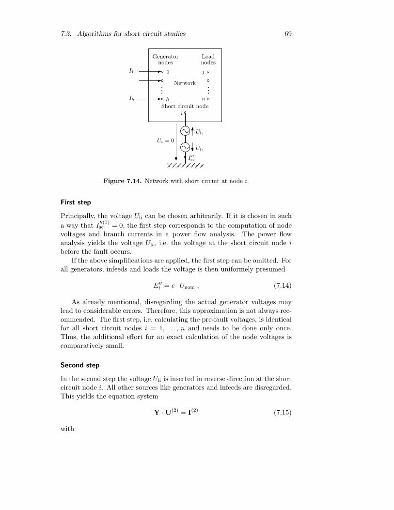
7.3. Algorithms for short circuit studies 69
I1
Ih
I ′′
sc
1
h
j
n
i
Generatornodes
Loadnodes
Short circuit node
Network
Ui = 0
Uli
Uli
Figure 7.14. Network with short circuit at node i.
First step
Principally, the voltage Uli can be chosen arbitrarily. If it is chosen in such
a way that I′′(1)sc = 0, the first step corresponds to the computation of node
voltages and branch currents in a power flow analysis. The power flowanalysis yields the voltage Uli, i.e. the voltage at the short circuit node ibefore the fault occurs.
If the above simplifications are applied, the first step can be omitted. Forall generators, infeeds and loads the voltage is then uniformely presumed
E′′i = c · Unom . (7.14)
As already mentioned, disregarding the actual generator voltages maylead to considerable errors. Therefore, this approximation is not always rec-ommended. The first step, i.e. calculating the pre-fault voltages, is identicalfor all short circuit nodes i = 1, . . . , n and needs to be done only once.Thus, the additional effort for an exact calculation of the node voltages iscomparatively small.
Second step
In the second step the voltage Uli is inserted in reverse direction at the shortcircuit node i. All other sources like generators and infeeds are disregarded.This yields the equation system
Y · U(2) = I(2) (7.15)
with
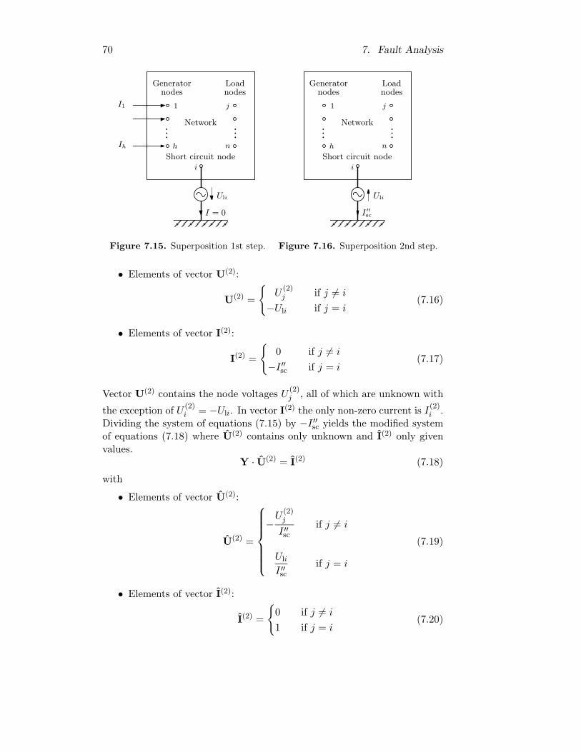
70 7. Fault Analysis
I1
Ih
1
h
j
n
i
Generatornodes
Loadnodes
Short circuit node
Network
Uli
I = 0
Figure 7.15. Superposition 1st step.
1
h
j
n
i
Generatornodes
Loadnodes
Short circuit node
Network
Uli
I ′′
sc
Figure 7.16. Superposition 2nd step.
• Elements of vector U(2):
U(2) =
U(2)j if j 6= i
−Uli if j = i(7.16)
• Elements of vector I(2):
I(2) =
0 if j 6= i
−I ′′sc if j = i(7.17)
Vector U(2) contains the node voltages U(2)j , all of which are unknown with
the exception of U(2)i = −Uli. In vector I(2) the only non-zero current is I
(2)i .
Dividing the system of equations (7.15) by −I ′′sc yields the modified systemof equations (7.18) where U(2) contains only unknown and I(2) only givenvalues.
Y · U(2) = I(2) (7.18)
with
• Elements of vector U(2):
U(2) =
−U
(2)j
I ′′scif j 6= i
Uli
I ′′scif j = i
(7.19)
• Elements of vector I(2):
I(2) =
0 if j 6= i
1 if j = i(7.20)
7.3. Algorithms for short circuit studies 71
The transformation from eq. (7.15) to eq. (7.18) leaves the admittancematrix Y unchanged. As a consequence, the triangular factorization of theadmittance matrix must be done only once, even if multiple short circuitcases are investigated. The superposition technique should therefore bepreferred to the direct solution of the linear system of equations (7.11).
However, if we compute the solution of eq. (7.18) with the known tech-nique, i.e. triangular factorization and forward-backward-substitution, a newforward-backward-substitution is required for every short circuit case. Thisdisadvantage can be avoided with the Takahashi method.
7.3.5 The Takahashi method
The principle idea behind the Takahashi method is the solution of eq. (7.18)by means of inversion. This yields
Z · I(2) = U(2) (7.21)
where
Z = Y−1 (7.22)
is the impedance matrix of the system. The unknown initial short circuitcurrent I ′′sc at node i can be found in the ith element of vector U(2)
U(2)i =
Uli
I ′′sc(7.23)
resp.
I ′′sc =Uli
U(2)i
. (7.24)
From eqs. (7.20) and (7.21) follows
U(2)i = zii (7.25)
where zii is an element on the main diagonal of matrix Z. Inserting eq. (7.25)in eq. (7.16) finally yields:
I ′′sc =Ui
zii(7.26)
For the calculation of the short circuit current only the main diagonalelement zii of the impedance matrix Z is required. Knowing all main diag-onal elements zii (i = 1, . . . , n) is therefore sufficient to compute the shortcircuit currents I ′′sci at all nodes i.
Often, also the partial short circuit currents Iji are to be determined.These are the currents that flow from adjacent nodes j to the short circuit
72 7. Fault Analysis
node i. With the simplification that all generator voltages are identical thepartial short circuit currents are
Iji =(
U(2)j − U
(2)i
)
yji
=(
U(2)j − U
(2)li
)
yji (7.27)
where yji is the admittance of the branch between j and i. If this simplifi-cation is not permitted the terms from the first step must be added here.
With eq. (7.21) follows:
Iji =(
−zji I′′sci + zii I
′′sci
)
yji
= I ′′sci (zii − zji) yji (7.28)
For the calculation of the partial short circuit currents from node j to theshort circuit node i in addition to the main diagonal element zii all elementszji are required. Because node j is connected directly to node i, the elementyji in the admittance matrix is non-zero. Although the impedance matrix Zis not sparse like the admittance matrix Y relatively few elements of Z mustbe known to calculate the short circuit currents and the partial short circuitcurrents for all nodes. Apart from the main diagonal elements zii these arethe elements zji that are non-zero in the corresponding admittance matrix.
In the Takahashi method only those elements of Z are determined thathave non-zero counterparts in the triangularly factorized admittance matrix.Except for the few fill-ins that emerge during factorization these are theelements of Z essential for the short circuit computation. The method shallbe demonstrated here:
Eq. (7.22) can be written as
Y · Z = E (7.29)
where E is the identity matrix. Y is factorized into triangular matrices andeq. (7.29) can be transformed in the following way:
L · D · R · Z = E | · L−1 (7.30)
D · R · Z = L−1 | · D−1
R · Z = D−1 · L−1 | + Z − R · ZZ = D−1 · L−1 + Z − R · ZZ = D−1 · L−1 + (E − R)Z (7.31)
The inverse of diagonal matrix D is again a diagonal matrix. Each elementon the main diagonal contains the reciprocal value of the element before the
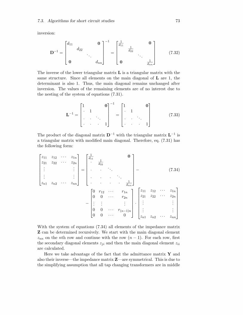
7.3. Algorithms for short circuit studies 73
inversion:
D−1 =
d11 0d22
. . .
0 dnn
−1
=
1d11
01
d22
. . .
0 1dnn
(7.32)
The inverse of the lower triangular matrix L is a triangular matrix with thesame structure. Since all elements on the main diagonal of L are 1, thedeterminant is also 1. Thus, the main diagonal remains unchanged afterinversion. The values of the remaining elements are of no interest due tothe nesting of the system of equations (7.31).
L−1 =
1 0· 1
· · . . .
· · · 1
−1
=
1 0· 1
· · . . .
· · · 1
(7.33)
The product of the diagonal matrix D−1 with the triangular matrix L−1 isa triangular matrix with modified main diagonal. Therefore, eq. (7.31) hasthe following form:
z11 z12 · · · z1n
z21 z22 · · · z2n...
......
...zn1 zn2 · · · znn
=
1d11
0
· 1d22
· · . . .
· · · . . .
· · · · 1dnn
− (7.34)
−
0 r12 · · · r1n
0 0 · · · r2n...
......
0 0 · · · r(n−1)n
0 0 · · · 0
·
z11 z12 · · · z1n
z21 z22 · · · z2n...
......
...zn1 zn2 · · · znn
With the system of equations (7.34) all elements of the impedance matrixZ can be determined recursively. We start with the main diagonal elementznn on the nth row and continue with the row (n − 1). For each row, firstthe secondary diagonal elements zji and then the main diagonal element zii
are calculated.
Here we take advantage of the fact that the admittance matrix Y andalso their inverse—the impedance matrix Z—are symmetrical. This is due tothe simplifying assumption that all tap changing transformers are in middle
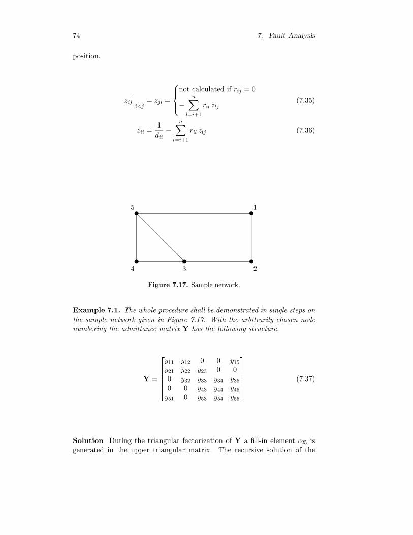
74 7. Fault Analysis
position.
zij
∣
∣
∣
i<j= zji =
not calculated if rij = 0
−n
∑
l=i+1
ril zlj(7.35)
zii =1
dii−
n∑
l=i+1
ril zlj (7.36)
@@
@@
@@
@@u
4
u5
u
3
u
2
u1
Figure 7.17. Sample network.
Example 7.1. The whole procedure shall be demonstrated in single steps onthe sample network given in Figure 7.17. With the arbitrarily chosen nodenumbering the admittance matrix Y has the following structure.
Y =
y11 y12 0 0 y15
y21 y22 y23 0 00 y32 y33 y34 y35
0 0 y43 y44 y45
y51 0 y53 y54 y55
(7.37)
Solution During the triangular factorization of Y a fill-in element c25 isgenerated in the upper triangular matrix. The recursive solution of the
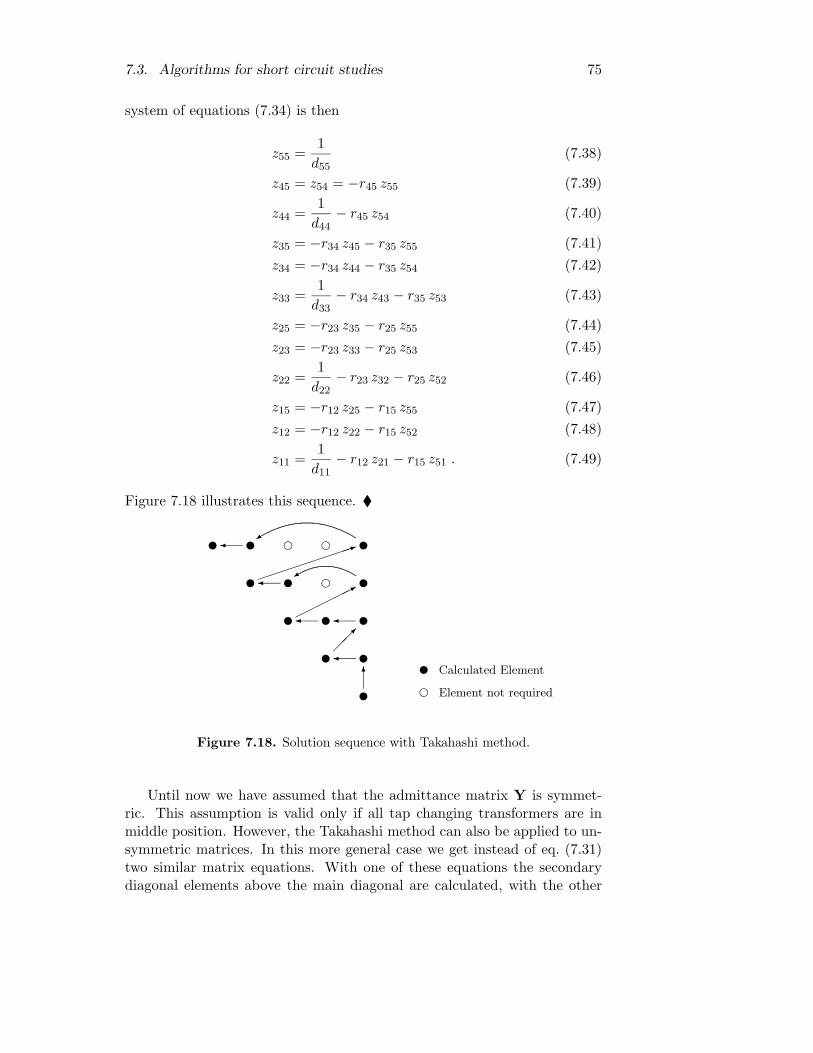
7.3. Algorithms for short circuit studies 75
system of equations (7.34) is then
z55 =1
d55(7.38)
z45 = z54 = −r45 z55 (7.39)
z44 =1
d44− r45 z54 (7.40)
z35 = −r34 z45 − r35 z55 (7.41)
z34 = −r34 z44 − r35 z54 (7.42)
z33 =1
d33− r34 z43 − r35 z53 (7.43)
z25 = −r23 z35 − r25 z55 (7.44)
z23 = −r23 z33 − r25 z53 (7.45)
z22 =1
d22− r23 z32 − r25 z52 (7.46)
z15 = −r12 z25 − r15 z55 (7.47)
z12 = −r12 z22 − r15 z52 (7.48)
z11 =1
d11− r12 z21 − r15 z51 . (7.49)
Figure 7.18 illustrates this sequence.
u
6
uu
uuu*u
+euu1 u
+eeuu
u Calculated Element
e Element not required
Figure 7.18. Solution sequence with Takahashi method.
Until now we have assumed that the admittance matrix Y is symmet-ric. This assumption is valid only if all tap changing transformers are inmiddle position. However, the Takahashi method can also be applied to un-symmetric matrices. In this more general case we get instead of eq. (7.31)two similar matrix equations. With one of these equations the secondarydiagonal elements above the main diagonal are calculated, with the other

76 7. Fault Analysis
equation the elements below the main diagonal. The elements on the maindiagonal can be calculated with either equation.
Unsymmetric matrices require about double the effort of symmetric ma-trices. Since neglecting the actual tap positions can lead to errors of 30 %,considering the actual tap positions is indicated for network operation ap-plications, that require short circuit computations with high accuracy.
Concluding remarks
The Takahashi method is an algorithm especially designed for the demandsof short circuit computations. Having the same accuracy it needs only afraction of the computation time of conventional methods. This advantageis important in real-time applications.
However, with the Takahashi method only the initial short circuit cur-rents can be calculated. This includes the partial short circuit currentsIji that flow from the adjacent nodes to the short circuit node i. It is notpossible to determine the short current shares delivered from individual gen-erators or infeeds. Thus the breaking current at the generators can not bedetermined with the Takahashi method but requires Gauss elimination.
Part II
Power System Dynamics and
Stability
77

8Classification and Definitions of Power
System Stability
This chapter contains a brief overview of some of the basic concepts in powersystem dynamics. A classification of different dynamic phenomena is givenand the requirements on modelling are discussed. Stability is a fundamentalconcept and a definition of stability in power systems is introduced. Insta-bilities in power systems can be classified according to their physical origins,and this classification is reviewed. Finally, a list of further reading in thesubject is given.
IN A ELECTRIC POWER SYSTEM a great variety of different dynam-ics occurs. These dynamic phenomena have different physical origin and
they occur in different time scales. A system is in a dynamic state if thetime derivative of any system quantity is non zero, and to describe a dy-namic system mathematically differential or difference equations must beemployed. As an example, the electric consumer loads in a power systemvary spontaneously all the time, and consequently one could state that thepower system is never in steady state in a strict mathematical sense. Sucha point of view is however unpractical in most cases, and one must, as whenit comes to most large and complex systems, study and analyse more or lesssimplified models of the system. To do relevant and adequate simplificationsis beneficial for the analysis, and contributes also to achieving results thatare easy to understand and easy to interpret. In addition, when derivingsimplified models one is forced to identify the most important processes andphenomena in the studied systems, which provides insight and deeper under-standing. Thus, as an example, the assumption that the loads are constantand that the electric power output from the generators are constant are rel-evant approximations for many studies of a power system, and the powersystem is under these assumptions described by a solution to the power flowequations. In the following we will refer to this state as the steady state ofthe power system.1
1In order to emphasise that this state is an approximation or idealisation, it is some-times referred to as quasi steady state. More generally, a quasi steady state is a state thatstrictly is a dynamic state, but could with sufficient accuracy be described by algebraic
79
80 8. Classification and Definitions of Power System Stability
8.1 Dynamics in Power Systems
There are a lot of different dynamical phenomena with different character-istics in a power system. The phenomena could be local, in which case theyonly involve a minor part of the system or a single component. But they canalso involve interactions between different parts of the system that might begeographically far from each other. In many cases these system-wide inter-actions are initiated by a local disturbance causing e.g. an earth fault withsubsequent change in network topology. In this compendium interactionsand phenomena that involve many power system components, e.g. genera-tors and loads, or parts of the system are dealt with. These interactionshave in common that they can cause system instabilities that can lead toblack outs in large parts of the system, i.e. to interruptions of power supplyfor many consumers.
Dynamics can also be initiated by actions of different controllers or byswitchings of lines or other components by system operators. Such “distur-bances” should be regarded as normal and should consequently not endangerthe stability of the system.
8.1.1 Classification of Dynamics
Dynamic phenomena in power systems are usually classified as
1. Electro-magnetic transients (100 Hz – MHz)
2. Electro-mechanical swings (rotor swings in synchronous machines) (0.1 –3 Hz)
3. Non-electric dynamics, e.g. mechanical phenomena and thermodynam-ics (up to tens of Hz)
Approximate values of typical frequencies are given in brackets.One single initial event in the power system can give rise to dynamics in
all the three groups above. A lightning stroke in a power line can induce sohigh over-voltages that the insulation fails, causing an earth fault. The earthfault can cause rotor swings in synchronous machines with high amplitudes.This can trigger protections to disconnect generators, so that an unbalancebetween produced and consumed power in the system arises. The frequencyin the system drops and generators participating in the frequency controlcompensate this by increasing their power outputs. Thus the initial lightningstroke has initiated dynamics in all the three groups above.
Another way to classify dynamic phenomena is given in Figure 8.1. Thisclassification is based on the time scale of the phenomenon and the (math-ematical) models used in analysis.
equations. One such example is fault current calculations, which often is done by usingalgebraic models even if it is a true dynamic phenomenon, see Figure 8.1.
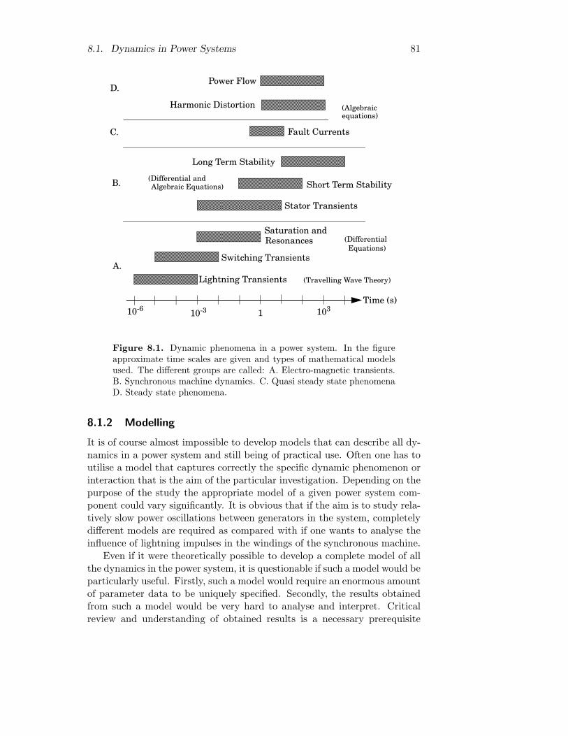
8.1. Dynamics in Power Systems 81
10-6 10-3 1 103Time (s)
Lightning Transients
Switching Transients
Saturation andResonances
(Travelling Wave Theory)
(DifferentialEquations)
Stator Transients
Short Term Stability
Long Term Stability
(Differential andAlgebraic Equations)
Fault Currents
Harmonic Distortion
Power Flow
(Algebraicequations)
A.
B.
C.
D.
Figure 8.1. Dynamic phenomena in a power system. In the figureapproximate time scales are given and types of mathematical modelsused. The different groups are called: A. Electro-magnetic transients.B. Synchronous machine dynamics. C. Quasi steady state phenomenaD. Steady state phenomena.
8.1.2 Modelling
It is of course almost impossible to develop models that can describe all dy-namics in a power system and still being of practical use. Often one has toutilise a model that captures correctly the specific dynamic phenomenon orinteraction that is the aim of the particular investigation. Depending on thepurpose of the study the appropriate model of a given power system com-ponent could vary significantly. It is obvious that if the aim is to study rela-tively slow power oscillations between generators in the system, completelydifferent models are required as compared with if one wants to analyse theinfluence of lightning impulses in the windings of the synchronous machine.
Even if it were theoretically possible to develop a complete model of allthe dynamics in the power system, it is questionable if such a model would beparticularly useful. Firstly, such a model would require an enormous amountof parameter data to be uniquely specified. Secondly, the results obtainedfrom such a model would be very hard to analyse and interpret. Criticalreview and understanding of obtained results is a necessary prerequisite
82 8. Classification and Definitions of Power System Stability
for sound engineering. When making simulations and computations, whichall are done with the help of computers nowadays in system sciences, it isimportant to have an expectation of what are reasonable outputs. Thustrivial errors due to wrong input data files, mistakes in modelling, etc. canbe eliminated to a large extent. The human factor is of utmost importancein computer-based analysis and simulation.
Models can in principle be erroneous in two different ways. Firstly, itcan have the wrong structure. It can be too simple overlooking importantinteractions and processes or modelling them incorrectly. This is of coursevery serious and might give rise to detrimental consequences. But it isalso very serious if wrong parameter data is used in a model of the correctstructure. This latter shortcoming occurs not seldom in technical systems,which might look surprising at first sight. Since technical systems are manmade, one should in principle have access to all design parameters definingthe system. But it turns out that many parameters, e.g. the gain in thecontroller, could easily be changed after the system has been commissionedand such changes are not always reported to system analysts. It is obviousthat the consequences could be very serious. In technical systems there are ofcourse parameters that are “genuinely” unknown, e.g. the ground resistivityunder a power line. In a large system like a power system, thousands ofparameters are needed to define the system completely. It is a very difficult,but also very important, task to maintain and keep the data bases whereall these parameter values are stored and updated. This is now a specialactivity usually referred to as data engineering.
In this compendium models needed for the problems to be analysed aredeveloped. Due to space limitations more detailed and elaborate derivationcannot be presented, but the reader is advised to consult other sources, e.g.books in electrical machines or the books listed at the end of this chapter.
8.2 Power System Stability
8.2.1 Definition of Stability
A dynamic phenomenon in a power system is, as said above, initiated bya disturbance in the system. Such a disturbance could as an example bethat a line impedance is changed due to an external cause. The behaviourof the system after this disturbance depends of course on a how “large”this disturbance is. A small disturbance results usually in small transientsin the system that are quickly damped out, while a larger disturbance willexcite larger oscillations. We all have an intuitive feeling for what is meantwith stability in this context. Stability is associated with that the systemoscillations decay and that the operation of the power systems can continuewithout any major impacts for any of the consumers. But, and this isvery important, as the power system is a nonlinear system (this will be
8.2. Power System Stability 83
elaborated on later) system stability depends on the kind and magnitude ofthe disturbance.2 This distinguishes nonlinear systems from linear systemsthat can be classified as stable or unstable independent of the disturbance,i.e. stability is a property of the linear system as such. As will be shownlater, stability of a power system is strongly coupled to both the magnitudeand character of the disturbance as well as to the initial operating point.
Over the years many different definitions of power system stability havebeen proposed. The most recent one, which will be adopted in these lecturenotes, was the result of a joint IEEE/CIGRE working group activity. In thereport in reference 7 of section 8.3, the following definition is given:
Definition 8.1. Power system stability is the ability of an electric powersystem, for a given initial operating condition, to regain a state of operatingequilibrium after being subjected to a physical disturbance, with most systemvariables bounded so that practically the entire system remains intact.
The following two comments elaborate on some important aspects of thisdefinition.
Comment 8.1. It is not necessary that the system regains the same steadystate operating equilibrium as prior to the disturbance. This would be thecase when e.g. the disturbance has caused any power system component (line,generator, etc.) to trip. Voltages and power flows will not be the same afterthe disturbance in such a case. Most disturbances that are considered instability analyses incur a change in system topology or structure.
Comment 8.2. It is important that the final steady state operating equi-librium after the fault is steady state acceptable. Otherwise protections orcontrol actions could introduce new disturbances that might influence the sta-bility of the system. Acceptable operating conditions must be clearly definedfor the power system under study.
As mentioned above there are also other definitions of power system sta-bility in the literature. They are not all identical, but could differ in somedetails, but most of them are in line with the definition proposed above.Power system dynamics can be modelled by systems of differential and al-gebraic equations, and the mathematics of those are studied in the theoryof dynamic systems. It is therefore desirable that the stability definitionsintroduced in a more mathematically stringent way are compatible with themore practically oriented definition above. In the report where the abovedefinition is proposed and motivated, these aspects are further discussed.
2To give an example of what is meant with magnitude in this context one could considera three phase to earth fault on a power line that is cleared by disconnecting the line. Themagnitude of this disturbance increases with the fault clearing time. If the fault clearingtime is sufficiently small, the system will remain stable, while a longer fault clearing mightcause system instability. Similarly, a high impedance fault gives a smaller disturbance thana solid fault.
84 8. Classification and Definitions of Power System Stability
8.2.2 Classification of Power System Stability
To achieve a better overview and structure of stability analyses of powersystems, it is of great help to classify possible power system stability. Theclassification to be introduced here is based on the physical mechanism be-ing the main driving force in the development of the associated instability.It could be either the active or the reactive power that is the importantquantity.
A common characteristic of the instabilities to be discussed here is thatthey have their origin in too large an imbalance of active or reactive power inthe system, locally or globally. This imbalance can then develop in differentways and cause unstable behaviour depending on system characteristics.Exactly what is meant with imbalance will be elaborated in the following.
Rotor Angular or Synchronous Stability
The total active electrical power fed into the power system by the generatorsis always equal to the active power consumed by the loads including thelosses in the system. On the other hand, there is not always a similarbalance between the loads and the power fed into the generators by theprime movers, e.g. the hydro and steam turbines. If such an imbalancedevelops, the rotating parts of the generators and other rotating machineswill act as energy buffer, and the kinetic energy stored in these will decreaseor increase as a result of the imbalance. Rotor angle stability refers to theability of synchronous machines of a power system to remain in synchronismafter a disturbance.
If the disturbance is local and substantial, e.g. an earth fault close to agenerator, the generator can fall out of step since it has been acceleratedduring the fault. As quite big currents will flow in the generator windingsin such a case, it must be disconnected to avoid that it is damaged. Typicaltime scale for such an instability to develop is a second to a couple of seconds.This kind of instability is called transient instability and instability appearsusually in form of aperiodic angular separation due to lack of synchronizingtorque. This form of instability is also referred to as large-disturbance rotorangle instability.
Small-disturbance (or small-signal) rotor angle stability is concernedwith the ability of the power system to maintain synchronism under smalldisturbances. These disturbances are considered to be sufficiently small thatlinearization of the system equations is permissible for purposes of analysis.Usually small-disturbance rotor angle stability is associated with insufficientdamping of oscillations.
8.2. Power System Stability 85
Frequency Stability
A third variety of active power imbalance, which is different from the onesabove, is when the imbalance is not local but global. In the preceding cases,the sum of active power infeed was enough but there was an imbalance lo-cally. But if the total power fed into the system by the prime movers isless than what is consumed by the loads, including losses, this imbalancewill influence the frequency of the whole system. As explained above thekinetic energy stored in rotating parts of the synchronous machines, andother rotating electrical machines, will compensate for the imbalance result-ing in a frequency deviation. If the imbalance is not too large the generatorsparticipating in the frequency control will regulate the active power inputfrom their prime movers, and bring back the frequency deviation to accept-able values. If the imbalance is too large, the frequency deviation will besignificant with possible serious consequences. Particularly thermal powerplants are sensitive to large frequency drops of long durations, since detri-mental oscillations could be excited in the turbines. As a last resort thegenerators are disconnected, making the situation even more serious. Thistype of instability is called frequency instability and the time scale could befrom a few seconds up to several minutes. Since the involved mechanismscould be quite different, one often distinguishes between short-term andlong-term frequency instability. In the latter, the control and protectionscharacteristics of turbines, boilers, and reactors play important roles.
Voltage Stability
When it comes to reactive power balance the situation is not as clear andsimple as concerning active power. There is always a balance between “pro-duced” and “consumed” reactive power in every node of a network. Thisis in fact a direct consequence of Kirchoff’s first current law. When onetalks about imbalance in this context we mean that the injected reactivepower is such, normally too small, that the voltage in the node cannot bekept to acceptable values. (At low load the injected reactive power couldbe high resulting in a too high voltage, possibly higher than the equipmentmight be designed for. This is of course not desirable but it could usuallybe controlled in such a way that no instabilities develop.) When we talkabout imbalance in this case we thus mean that the injected reactive powerdiffers from the desired injected reactive power, needed to keep the desiredvoltage. If this imbalance gets too high, the voltages exceed the acceptablerange.
Reactive power is a more local quantity than active power since it can-not be transported as easily in power system where normally X ≫ R. Thisexplains why voltage problems often are local, and often only occur in partof the system. When the imbalances (voltage problems) develop into insta-
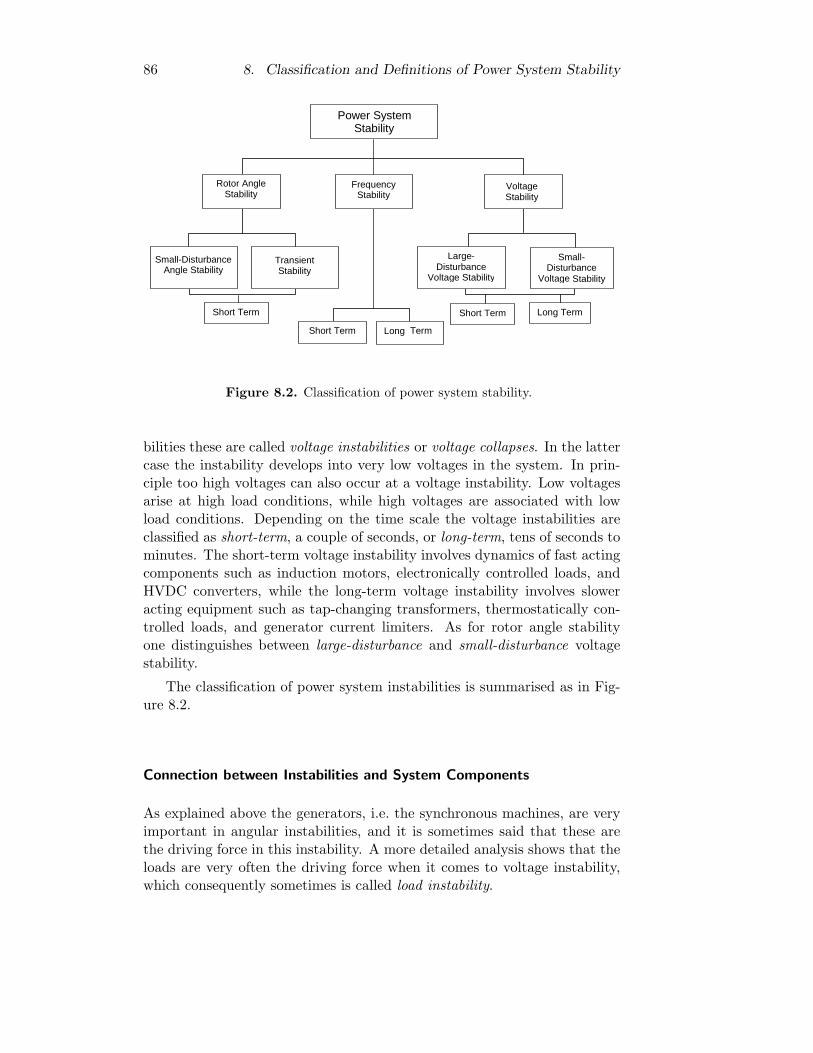
86 8. Classification and Definitions of Power System Stability
Short Term
Small - Disturbance Angle Stability
Transient Stability
Large - Disturbance
Voltage Stability
Small - Disturbance
Voltage Stability
Short Term Long Term
Power System Stability
Rotor Angle Stability
Frequency Stability
Voltage Stability
Long Term Short Term
Figure 8.2. Classification of power system stability.
bilities these are called voltage instabilities or voltage collapses. In the lattercase the instability develops into very low voltages in the system. In prin-ciple too high voltages can also occur at a voltage instability. Low voltagesarise at high load conditions, while high voltages are associated with lowload conditions. Depending on the time scale the voltage instabilities areclassified as short-term, a couple of seconds, or long-term, tens of seconds tominutes. The short-term voltage instability involves dynamics of fast actingcomponents such as induction motors, electronically controlled loads, andHVDC converters, while the long-term voltage instability involves sloweracting equipment such as tap-changing transformers, thermostatically con-trolled loads, and generator current limiters. As for rotor angle stabilityone distinguishes between large-disturbance and small-disturbance voltagestability.
The classification of power system instabilities is summarised as in Fig-ure 8.2.
Connection between Instabilities and System Components
As explained above the generators, i.e. the synchronous machines, are veryimportant in angular instabilities, and it is sometimes said that these arethe driving force in this instability. A more detailed analysis shows that theloads are very often the driving force when it comes to voltage instability,which consequently sometimes is called load instability.
8.3. Literature on Power System Dynamics and Stability 87
Instabilities in Real Systems
The classification above is based on simplified and ideal conditions in thesystem. In a real system these assumptions might not be valid. In realsystems it is not seldom a combination of active and reactive power imbal-ances that trigger an instability. However, in many cases it is possible toidentify which is the dominating processes in the beginning of the instabil-ity. During the course of the dynamics new consequential imbalances mightoccur, resulting in a combined angular and voltage instability in the finalphase. There are examples of black outs in power systems that have startedas slow voltage instabilities, which through low voltages have reduced thepower transfer capability resulting in rotor angular instabilities causing thefinal collapse of the system. On the other hand, rotor angular instabili-ties can cause generators to trip, which most systems are designed to copewith, but it can effect the reactive power balance in such a way that voltageinstabilities can develop.
The purpose of a classification is to define a structure for a complicatedproblem and thereby better understanding it. Furthermore it often helps toidentify important and critical quantities, processes and components in thesystem. Classifications of this kind should not be driven too far. Most im-portant is always that useful and adequate results are obtained from realisticmodels of the power system.
8.3 Literature on Power System Dynamics and Sta-
bility
These lecture notes should be seen as an introduction to power system dy-namics and stability. For those who want to get deeper knowledge in thesubject there are a number of books that can be recommended. They haveall their strong and weaker sides, and one has often to consult several booksto get a complete view of a problem. Below are only references listed thatare fairly modern and focus on power system dynamics and stability.
1. Power System Stability and Control by Prabha Kundur. (McGraw-Hill Inc., 1994, ISBN 0-07-035958-X, 1176 pages)This is the most complete modern book on the subject and is alreadya classic textbook. It covers most subtopics and its approach is ratherpractical, but it contains a fair amount of theory also. The bookcontains a lot of references to other books and published papers.
2. Power System Dynamics and Stability by Jan Machowski, Janusz W.Bialek and James R. Bumby. (John Wiley & Sons Ltd, 1997, ISBN0-471-97174-X, 461 pages)This book does not contain as many applications as the previous one.
88 8. Classification and Definitions of Power System Stability
On the other hand, it contains rather detailed motivations and deriva-tions of many of the basic assumptions in power system analysis. Alarge part of the book is devoted to control and supervision of powersystems.
3. Power Systems Dynamics. Stability and Control by K. R. Padiyar.(John Wiley & Sons Ltd, 1996, ISBN 0-471-19002-0, 629 pages)The book gives a good overview with many solved problems. Thefocus is on angular stability, while voltage stability is on briefly dealtwith.
4. Power System Dynamics and Stability by Peter W. Sauer and M. A.Pai. (Prentice Hall, 1998, ISBN 0-13-678830-0, 357 pages) The mathe-matical level in this book is higher than the previous ones and to fullyappreciate it knowledge in the theory of nonlinear systems is needed.Only angular stability is included.
5. Power System Voltage Stability by Carson W. Taylor. (McGraw-HillInc., 1994, ISBN 0-07-063184-0, 273 pages) This book deals only withvoltage stability. The approach is rather practical. Many examplesfrom voltage instabilities in real systems are reviewed and analysed.
6. Voltage Stability of Electric Power Systems by Thierry Van Cutsemand Costas Vournas. (Kluwer Academic Publishers, 1998, ISBN 0-7923-8139-4, 378 pages) Voltage stability is the subject of this bookalso. However the approach is more mathematical than in the previousone, and to fully appreciate it, knowledge about nonlinear systems isrequired.
7. Definition and Classification of Power System Stability IEEE/CIGREJoint Task Force on Stability Terms and Definitions, 2002.
9Synchronous Machine Models
This chapter starts with a short discussion that motivates why synchronousmachines are important when electro-mechanical oscillations are studied. Abrief overview of the operating principles and design of the synchronous ma-chine is given. This forms the basis of simplified models that are derived –first for stationary, then for dynamic operation. Even if the dynamic modelis very simple and neglects a number of features, it captures the most impor-tant properties to model electro-mechanical oscillations in power systems.
SYNCHRONOUS MACHINES, i.e. practically all generators together withsynchronous motors and synchronous compensators, are the most impor-
tant power system components in the analysis of electro-mechanical oscilla-tions in power systems. The oscillations are manifested in that the rotorsof the synchronous machines do not rotate with constant angular velocitycorresponding to system frequency, but superimposed are low frequency os-cillations, typically 0.1 – 4 Hz. It is important that these superimposedoscillations are not too large, because then the stability of the power systemcan be endangered. A correct description of these oscillations often requiresdetailed models of many different system components, but to get an un-derstanding of and insight into the basic physical phenomena and processesthat determine the stability it is often sufficient to employ the simple modelthat will be derived and motivated in this chapter. This simplified model ofthe synchronous machine together with a simple model of the power trans-mission system provide a description that will be used in chapter 11.
As the name electro-mechanical oscillations suggests, both electrical andmechanical phenomena are involved, i.e. both currents in and voltages acrossdifferent windings in the machines but also the mechanical motion of therotor. Therefore, models of both electrical and mechanical parts of thesynchronous machine are needed.
9.1 Design and Operating Principle
In the synchronous machine a magnetized rotor creates a rotating magneticfield in the air gap. If the rotor field is ideally sinusoidal and if the rotorrotates at constant speed, this will induce ideally sinusoidal voltages in the
89
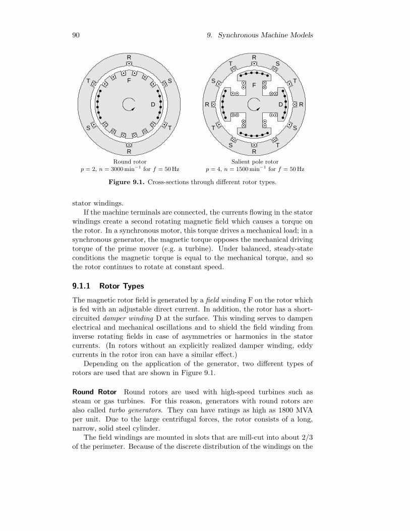
90 9. Synchronous Machine Models
R
S
T
R
S
T F
D
Round rotorp = 2, n = 3000 min−1 for f = 50Hz
RS
T
R
S
TR
S
T
R
S
T
F
D
Salient pole rotorp = 4, n = 1500min−1 for f = 50 Hz
Figure 9.1. Cross-sections through different rotor types.
stator windings.If the machine terminals are connected, the currents flowing in the stator
windings create a second rotating magnetic field which causes a torque onthe rotor. In a synchronous motor, this torque drives a mechanical load; in asynchronous generator, the magnetic torque opposes the mechanical drivingtorque of the prime mover (e.g. a turbine). Under balanced, steady-stateconditions the magnetic torque is equal to the mechanical torque, and sothe rotor continues to rotate at constant speed.
9.1.1 Rotor Types
The magnetic rotor field is generated by a field winding F on the rotor whichis fed with an adjustable direct current. In addition, the rotor has a short-circuited damper winding D at the surface. This winding serves to dampenelectrical and mechanical oscillations and to shield the field winding frominverse rotating fields in case of asymmetries or harmonics in the statorcurrents. (In rotors without an explicitly realized damper winding, eddycurrents in the rotor iron can have a similar effect.)
Depending on the application of the generator, two different types ofrotors are used that are shown in Figure 9.1.
Round Rotor Round rotors are used with high-speed turbines such assteam or gas turbines. For this reason, generators with round rotors arealso called turbo generators. They can have ratings as high as 1800 MVAper unit. Due to the large centrifugal forces, the rotor consists of a long,narrow, solid steel cylinder.
The field windings are mounted in slots that are mill-cut into about 2/3of the perimeter. Because of the discrete distribution of the windings on the
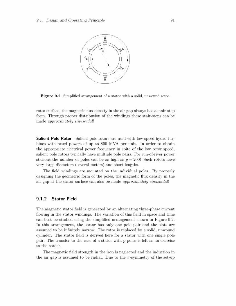
9.1. Design and Operating Principle 91
R
S
T
R
S
Tα
δ
Figure 9.2. Simplified arrangement of a stator with a solid, unwound rotor.
rotor surface, the magnetic flux density in the air gap always has a stair-stepform. Through proper distribution of the windings these stair-steps can bemade approximately sinusoidal !
Salient Pole Rotor Salient pole rotors are used with low-speed hydro tur-bines with rated powers of up to 800 MVA per unit. In order to obtainthe appropriate electrical power frequency in spite of the low rotor speed,salient pole rotors typically have multiple pole pairs. For run-of-river powerstations the number of poles can be as high as p = 200! Such rotors havevery large diameters (several meters) and short lengths.
The field windings are mounted on the individual poles. By properlydesigning the geometric form of the poles, the magnetic flux density in theair gap at the stator surface can also be made approximately sinusoidal !
9.1.2 Stator Field
The magnetic stator field is generated by an alternating three-phase currentflowing in the stator windings. The variation of this field in space and timecan best be studied using the simplified arrangement shown in Figure 9.2.In this arrangement, the stator has only one pole pair and the slots areassumed to be infinitely narrow. The rotor is replaced by a solid, unwoundcylinder. The stator field is derived here for a stator with one single polepair. The transfer to the case of a stator with p poles is left as an exerciseto the reader.
The magnetic field strength in the iron is neglected and the induction inthe air gap is assumed to be radial. Due to the π-symmetry of the set-up
92 9. Synchronous Machine Models
Ampere’s law gives for the dotted path shown in Figure 9.2
Θ(α) =
∫∫
A(α)
~i d~a =1
µ0
∮
S(α)
~B d~s =B(α)
µ0· 2 · δ (9.1)
where A(α) is the area enclosed by the path, δ is the width of the air gap,B(α) is the flux density in the air gap at the angle α, and Θ(α) is the totalflux linkage (or number of ampere windings) enclosed by the path.
One single-phase winding If only phase R is fed by an alternating current,the total enclosed flux linkage is either +w · iR(t) or −w · iR(t), dependingon whether the path encloses the upper slot (0 < α < π) or the lower one(π < α < 2π). w is the number of windings in one slot.
The left side of Figure 9.3 shows the flux linkage of a single-phase windingplotted against the angle α for different instants of time. Since B(α) isdirectly proportional to Θ(α) as shown in eq. (9.1), the magnetic field in theair gap is a rectangular, standing wave with a variable amplitude.
Three-phase windings If the three phases R, S and T are fed by an al-ternating three-phase current, the integration path in Figure 9.2 alwaysencloses three slots that carry windings with different momentary currents.The resulting total flux as a function of the angle α is thus a superpositionof three rectangular curves that are shifted by 2/3 · π and have differentamplitudes.
This is shown on the right side of Figure 9.3. It is evident that thefundamental component of the total flux is a traveling wave with a constantamplitude which moves with the angular velocity ω. This angular velocityof the stator field is the same as the angular frequency of the alternatingcurrents. In a real stator, the windings are of course not concentrated ininfinitely narrow slots. Instead, they are distributed among several slotsof finite extent – possibly with a different number of windings in differentslots. Through proper design the magnetic field in the air gap can be madeapproximately sinusoidal.
It should be noted that this simplified treatment of the stator field is onlyapplicable for generators with round rotors where the air gap has a constantwidth. In the case of a salient pole rotor, the width of the air gap is variable,and therefore the magnetic stator field depends not only on the momentarywinding currents but also on the momentary rotational angle of the rotor.In some cases, the differences between round rotor and salient pole rotor canbe neglected (as will be done frequently in the remainder of this chapter).However, it should be kept in mind that this is a simplification which needsto be justified from case to case.
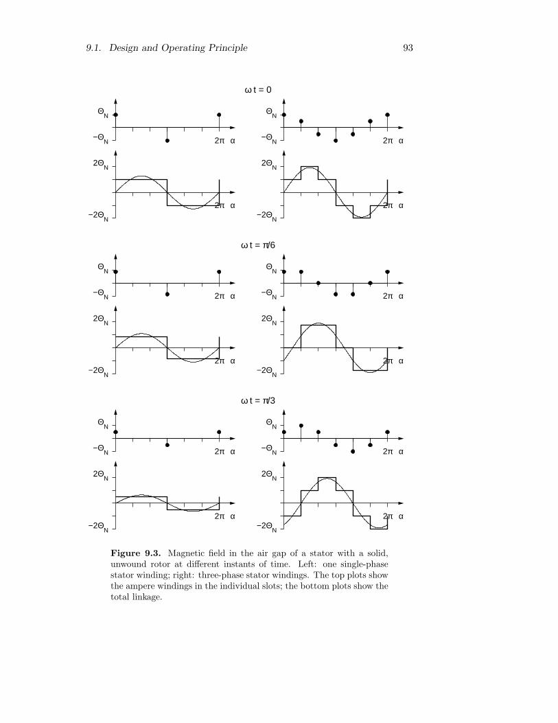
9.1. Design and Operating Principle 93
α2π−ΘN
ΘN
ω t = π/3
α2π−2Θ
N
2ΘN
α2π−ΘN
ΘN
ω t = π/6
α2π−2Θ
N
2ΘN
α2π−ΘN
ΘN
ω t = 0
α2π−2Θ
N
2ΘN
α2π−ΘN
ΘN
α2π−2Θ
N
2ΘN
α2π−ΘN
ΘN
α2π−2Θ
N
2ΘN
α2π−ΘN
ΘN
α2π−2Θ
N
2ΘN
Figure 9.3. Magnetic field in the air gap of a stator with a solid,unwound rotor at different instants of time. Left: one single-phasestator winding; right: three-phase stator windings. The top plots showthe ampere windings in the individual slots; the bottom plots show thetotal linkage.
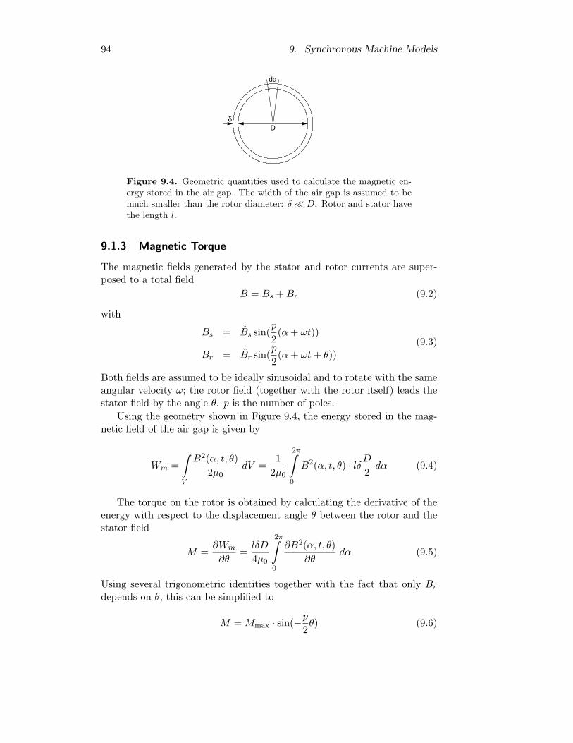
94 9. Synchronous Machine Models
dα
δD
Figure 9.4. Geometric quantities used to calculate the magnetic en-ergy stored in the air gap. The width of the air gap is assumed to bemuch smaller than the rotor diameter: δ ≪ D. Rotor and stator havethe length l.
9.1.3 Magnetic Torque
The magnetic fields generated by the stator and rotor currents are super-posed to a total field
B = Bs + Br (9.2)
with
Bs = Bs sin(p
2(α + ωt))
Br = Br sin(p
2(α + ωt + θ))
(9.3)
Both fields are assumed to be ideally sinusoidal and to rotate with the sameangular velocity ω; the rotor field (together with the rotor itself) leads thestator field by the angle θ. p is the number of poles.
Using the geometry shown in Figure 9.4, the energy stored in the mag-netic field of the air gap is given by
Wm =
∫
V
B2(α, t, θ)
2µ0dV =
1
2µ0
2π∫
0
B2(α, t, θ) · lδD
2dα (9.4)
The torque on the rotor is obtained by calculating the derivative of theenergy with respect to the displacement angle θ between the rotor and thestator field
M =∂Wm
∂θ=
lδD
4µ0
2π∫
0
∂B2(α, t, θ)
∂θdα (9.5)
Using several trigonometric identities together with the fact that only Br
depends on θ, this can be simplified to
M = Mmax · sin(−p
2θ) (9.6)
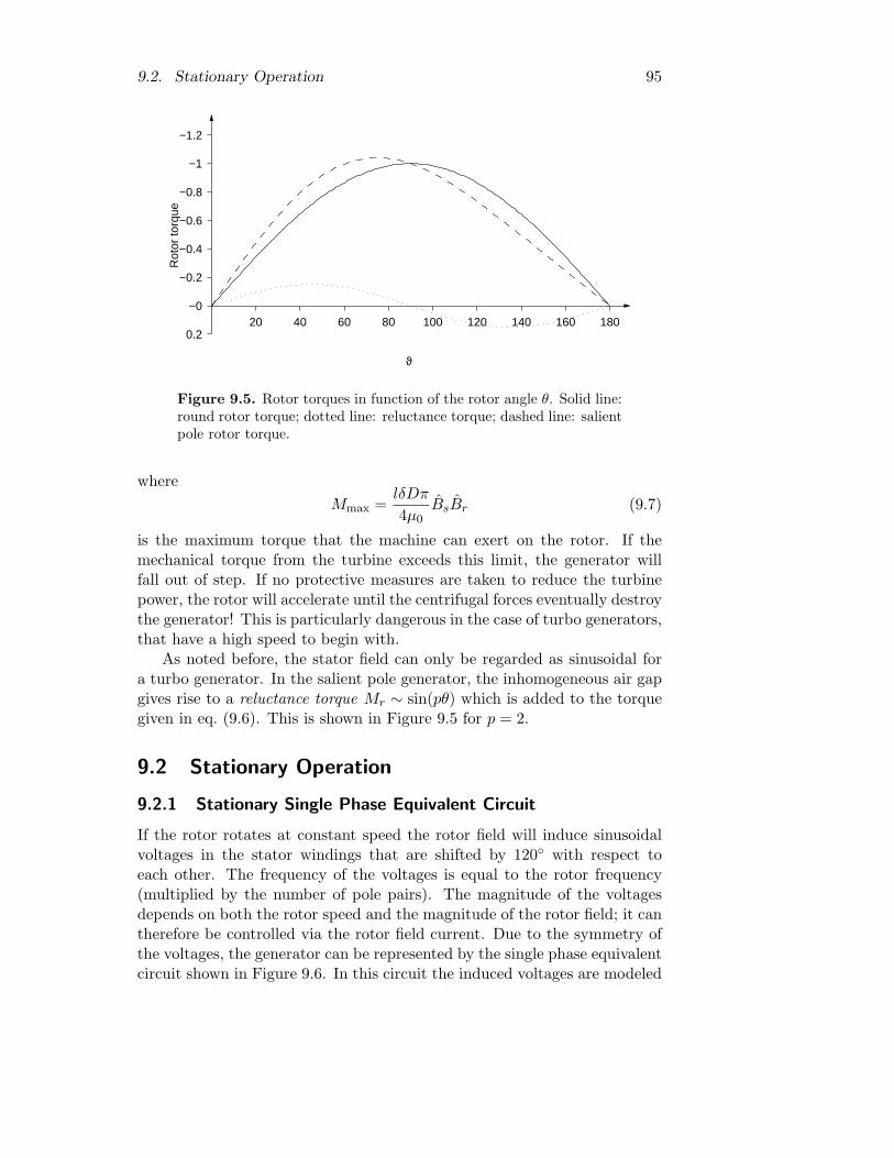
9.2. Stationary Operation 95
ϑ
Rot
or to
rque
20 40 60 80 100 120 140 160 1800.2
−0
−0.2
−0.4
−0.6
−0.8
−1
−1.2
Figure 9.5. Rotor torques in function of the rotor angle θ. Solid line:round rotor torque; dotted line: reluctance torque; dashed line: salientpole rotor torque.
where
Mmax =lδDπ
4µ0BsBr (9.7)
is the maximum torque that the machine can exert on the rotor. If themechanical torque from the turbine exceeds this limit, the generator willfall out of step. If no protective measures are taken to reduce the turbinepower, the rotor will accelerate until the centrifugal forces eventually destroythe generator! This is particularly dangerous in the case of turbo generators,that have a high speed to begin with.
As noted before, the stator field can only be regarded as sinusoidal fora turbo generator. In the salient pole generator, the inhomogeneous air gapgives rise to a reluctance torque Mr ∼ sin(pθ) which is added to the torquegiven in eq. (9.6). This is shown in Figure 9.5 for p = 2.
9.2 Stationary Operation
9.2.1 Stationary Single Phase Equivalent Circuit
If the rotor rotates at constant speed the rotor field will induce sinusoidalvoltages in the stator windings that are shifted by 120 with respect toeach other. The frequency of the voltages is equal to the rotor frequency(multiplied by the number of pole pairs). The magnitude of the voltagesdepends on both the rotor speed and the magnitude of the rotor field; it cantherefore be controlled via the rotor field current. Due to the symmetry ofthe voltages, the generator can be represented by the single phase equivalentcircuit shown in Figure 9.6. In this circuit the induced voltages are modeled
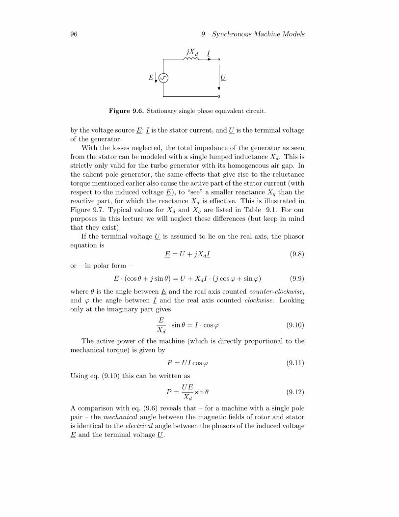
96 9. Synchronous Machine Models
E
jX d I
U
Figure 9.6. Stationary single phase equivalent circuit.
by the voltage source E; I is the stator current, and U is the terminal voltageof the generator.
With the losses neglected, the total impedance of the generator as seenfrom the stator can be modeled with a single lumped inductance Xd. This isstrictly only valid for the turbo generator with its homogeneous air gap. Inthe salient pole generator, the same effects that give rise to the reluctancetorque mentioned earlier also cause the active part of the stator current (withrespect to the induced voltage E), to “see” a smaller reactance Xq than thereactive part, for which the reactance Xd is effective. This is illustrated inFigure 9.7. Typical values for Xd and Xq are listed in Table 9.1. For ourpurposes in this lecture we will neglect these differences (but keep in mindthat they exist).
If the terminal voltage U is assumed to lie on the real axis, the phasorequation is
E = U + jXdI (9.8)
or – in polar form –
E · (cos θ + j sin θ) = U + XdI · (j cos ϕ + sinϕ) (9.9)
where θ is the angle between E and the real axis counted counter-clockwise,and ϕ the angle between I and the real axis counted clockwise. Lookingonly at the imaginary part gives
E
Xd· sin θ = I · cos ϕ (9.10)
The active power of the machine (which is directly proportional to themechanical torque) is given by
P = UI cos ϕ (9.11)
Using eq. (9.10) this can be written as
P =UE
Xdsin θ (9.12)
A comparison with eq. (9.6) reveals that – for a machine with a single polepair – the mechanical angle between the magnetic fields of rotor and statoris identical to the electrical angle between the phasors of the induced voltageE and the terminal voltage U .
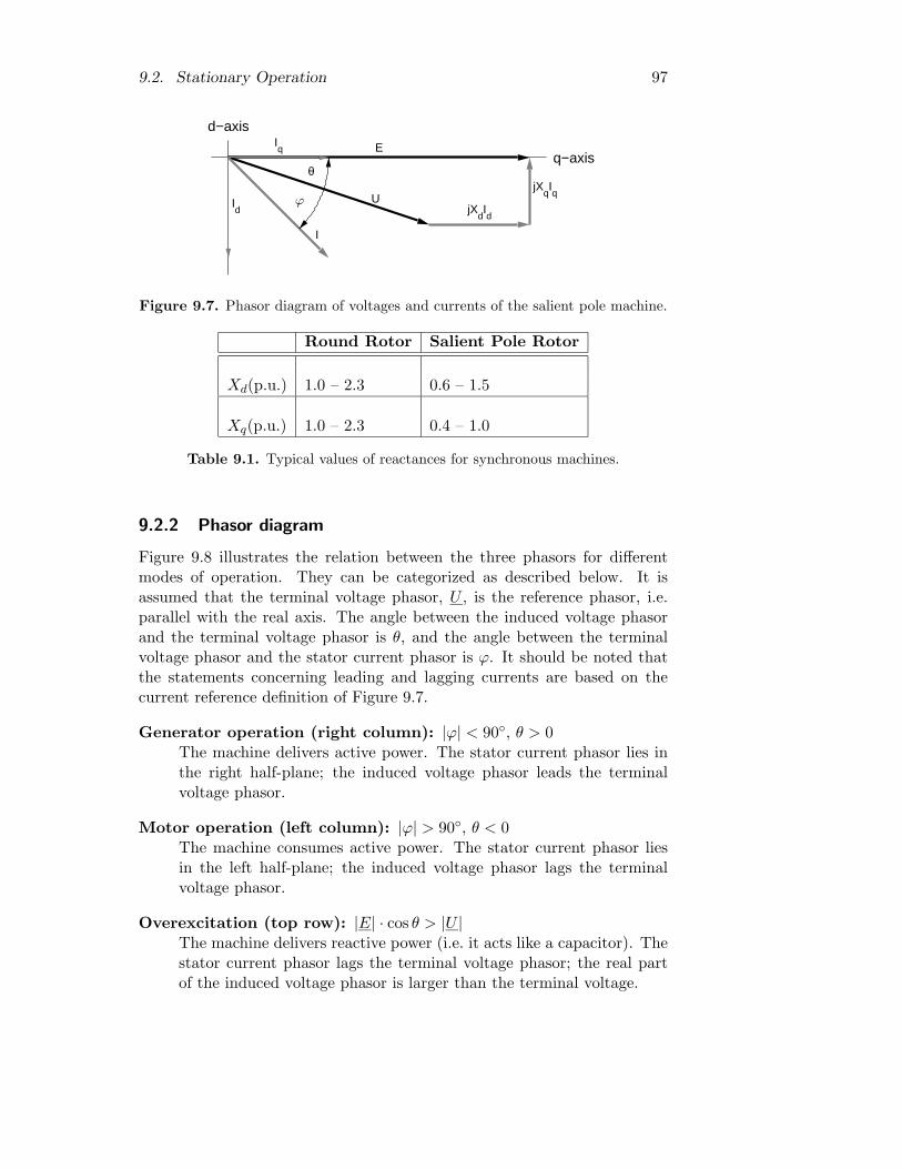
9.2. Stationary Operation 97
d−axis
q−axisE
U
I
jXdId
jXqIq
Iq
Id
θ
ϕ
Figure 9.7. Phasor diagram of voltages and currents of the salient pole machine.
Round Rotor Salient Pole Rotor
Xd(p.u.) 1.0 – 2.3 0.6 – 1.5
Xq(p.u.) 1.0 – 2.3 0.4 – 1.0
Table 9.1. Typical values of reactances for synchronous machines.
9.2.2 Phasor diagram
Figure 9.8 illustrates the relation between the three phasors for differentmodes of operation. They can be categorized as described below. It isassumed that the terminal voltage phasor, U , is the reference phasor, i.e.parallel with the real axis. The angle between the induced voltage phasorand the terminal voltage phasor is θ, and the angle between the terminalvoltage phasor and the stator current phasor is ϕ. It should be noted thatthe statements concerning leading and lagging currents are based on thecurrent reference definition of Figure 9.7.
Generator operation (right column): |ϕ| < 90, θ > 0The machine delivers active power. The stator current phasor lies inthe right half-plane; the induced voltage phasor leads the terminalvoltage phasor.
Motor operation (left column): |ϕ| > 90, θ < 0The machine consumes active power. The stator current phasor liesin the left half-plane; the induced voltage phasor lags the terminalvoltage phasor.
Overexcitation (top row): |E| · cos θ > |U |The machine delivers reactive power (i.e. it acts like a capacitor). Thestator current phasor lags the terminal voltage phasor; the real partof the induced voltage phasor is larger than the terminal voltage.
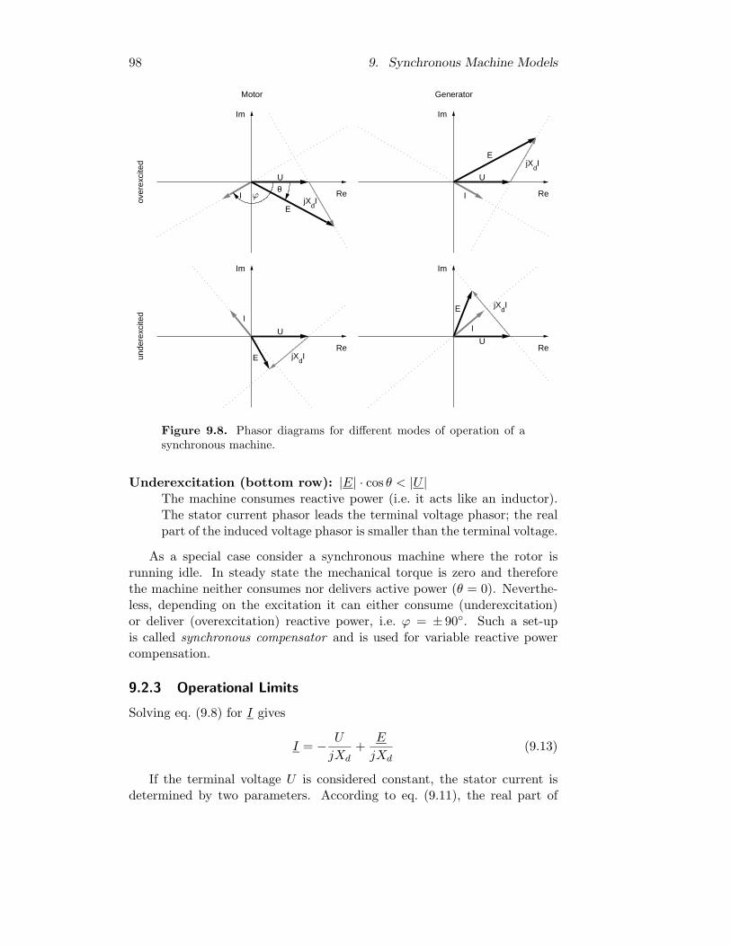
98 9. Synchronous Machine Models
Re
Im
U
E
IjX
dI
Motor
over
exci
ted
θ
Re
Im
U
E
I
jXdIun
dere
xcite
d
Re
Im
U
E
I
jXdI
Generator
Re
Im
U
E
I
jXdI
ϕ
Figure 9.8. Phasor diagrams for different modes of operation of asynchronous machine.
Underexcitation (bottom row): |E| · cos θ < |U |The machine consumes reactive power (i.e. it acts like an inductor).The stator current phasor leads the terminal voltage phasor; the realpart of the induced voltage phasor is smaller than the terminal voltage.
As a special case consider a synchronous machine where the rotor isrunning idle. In steady state the mechanical torque is zero and thereforethe machine neither consumes nor delivers active power (θ = 0). Neverthe-less, depending on the excitation it can either consume (underexcitation)or deliver (overexcitation) reactive power, i.e. ϕ = ± 90. Such a set-upis called synchronous compensator and is used for variable reactive powercompensation.
9.2.3 Operational Limits
Solving eq. (9.8) for I gives
I = − U
jXd+
E
jXd(9.13)
If the terminal voltage U is considered constant, the stator current isdetermined by two parameters. According to eq. (9.11), the real part of
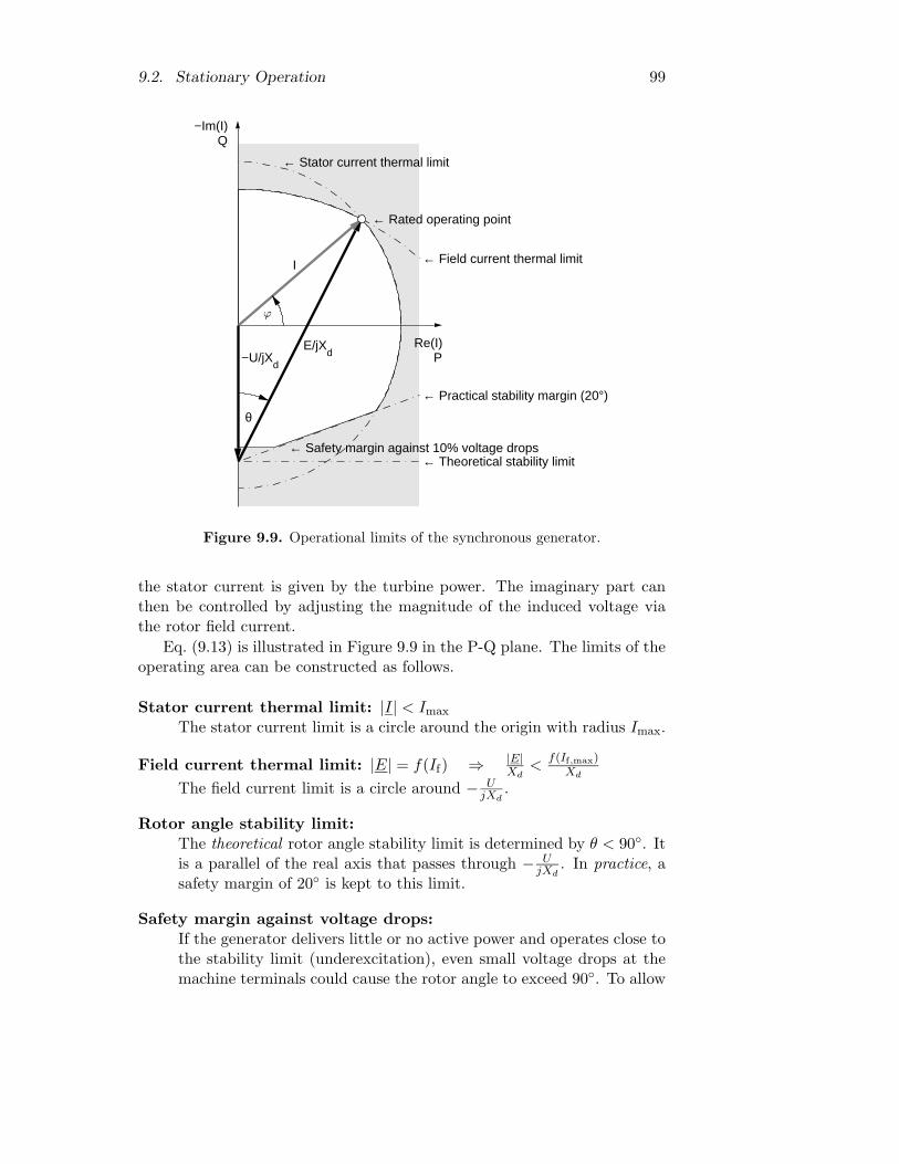
9.2. Stationary Operation 99
Re(I)P
−Im(I)Q
← Stator current thermal limit
← Field current thermal limit
← Theoretical stability limit
← Practical stability margin (20°)
← Safety margin against 10% voltage drops
E/jXd
I
−U/jXd
← Rated operating point
θ
ϕ
Figure 9.9. Operational limits of the synchronous generator.
the stator current is given by the turbine power. The imaginary part canthen be controlled by adjusting the magnitude of the induced voltage viathe rotor field current.
Eq. (9.13) is illustrated in Figure 9.9 in the P-Q plane. The limits of theoperating area can be constructed as follows.
Stator current thermal limit: |I| < Imax
The stator current limit is a circle around the origin with radius Imax.
Field current thermal limit: |E| = f(If) ⇒ |E|Xd
<f(If,max)
Xd
The field current limit is a circle around − UjXd
.
Rotor angle stability limit:The theoretical rotor angle stability limit is determined by θ < 90. Itis a parallel of the real axis that passes through − U
jXd. In practice, a
safety margin of 20 is kept to this limit.
Safety margin against voltage drops:If the generator delivers little or no active power and operates close tothe stability limit (underexcitation), even small voltage drops at themachine terminals could cause the rotor angle to exceed 90. To allow
100 9. Synchronous Machine Models
for 10 % voltage drops, the operating point must stay above a parallelof the real axis passing through −0.9 · U
jXd.
Depending on the design of the generator, there may be other limiting factors(e.g. for turbo generators the stator end region heating limit mentioned insection 2.5).
9.3 Dynamic Operation
9.3.1 Transient Single Phase Equivalent Circuit
During network transients, the reactance of the synchronous generator is notconstant. For symmetrical transients, as discussed in section 7.2 on shortcircuits of synchronous machines, the machine reactance itself undergoestransient changes as the machine passes through the sub-transient, transient,and steady-state stages. In the fault analysis in chapter 7, only the first fewcycles after a fault were of interest. The generator was therefore modeledwith the sub-transient reactance X ′′
d .Compared to the time scale of short-circuit overcurrents, electro-mechan-
ical oscillations are much slower (0.1 – 4 Hz as mentioned in the introductionto this chapter). For the study of these phenomena, the sub-transient phaseis therefore neglected and the generator is modeled with the transient reac-tance X ′
d. Similarly, during transients, the magnitude of the induced voltagedrops to the value E′ which can be calculated as follows
E′ =X ′
d
Xd· E0 +
Xd − X ′d
Xd· U0 · cos θ0 (9.14)
orE′ = E0 − (Xd − X ′
d) · I0 · sinϕ0 (9.15)
where the superscript 0 denotes the steady-state quantities prior to the tran-sient.
Thus, the phasor equation valid during network transients is
E′ = U + jX ′dI (9.16)
9.3.2 Simplified Mechanical Model
As stated above the rotor of a synchronous machine rotates with synchronousspeed in steady state. If the electrical frequency of the system is ωe, themechanical angular velocity ωm of the rotor is given by
ωm =ωe
p/2(9.17)
where p is the number of poles of the machine.
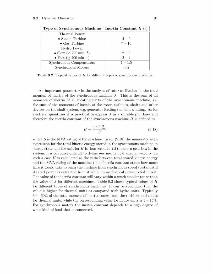
9.3. Dynamic Operation 101
Type of Synchronous Machine Inertia Constant H (s)
Thermal Power• Steam Turbine 4 – 9• Gas Turbine 7 – 10
Hydro Power• Slow (< 200 min−1) 2 – 3• Fast (≥ 200 min−1) 2 – 4
Synchronous Compensators 1 – 1.5
Synchronous Motors ≈ 2
Table 9.2. Typical values of H for different types of synchronous machines.
An important parameter in the analysis of rotor oscillations is the totalmoment of inertia of the synchronous machine J . This is the sum of allmoments of inertia of all rotating parts of the synchronous machine, i.e.the sum of the moments of inertia of the rotor, turbines, shafts and otherdevices on the shaft system, e.g. generator feeding the field winding. As forelectrical quantities it is practical to express J in a suitable p.u. base andtherefore the inertia constant of the synchronous machine H is defined as
H =0.5Jω2
mo
S(9.18)
where S is the MVA rating of the machine. In eq. (9.18) the numerator is anexpression for the total kinetic energy stored in the synchronous machine insteady state and the unit for H is thus seconds. (If there is a gear box in thesystem, it is of course difficult to define one mechanical angular velocity. Insuch a case H is calculated as the ratio between total stored kinetic energyand the MVA rating of the machine.) The inertia constant states how muchtime it would take to bring the machine from synchronous speed to standstillif rated power is extracted from it while no mechanical power is fed into it.The value of the inertia constant will vary within a much smaller range thanthe value of J for different machines. Table 9.2 shows typical values of Hfor different types of synchronous machines. It can be concluded that thevalue is higher for thermal units as compared with hydro units. Typically30 – 60% of the total moment of inertia comes from the turbines and shaftsfor thermal units, while the corresponding value for hydro units is 5 – 15%.For synchronous motors the inertia constant depends to a high degree ofwhat kind of load that is connected.

102 9. Synchronous Machine Models
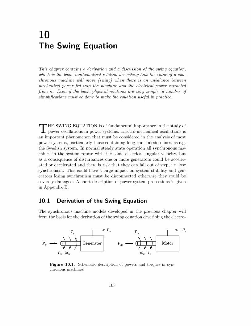
10The Swing Equation
This chapter contains a derivation and a discussion of the swing equation,which is the basic mathematical relation describing how the rotor of a syn-chronous machine will move (swing) when there is an unbalance betweenmechanical power fed into the machine and the electrical power extractedfrom it. Even if the basic physical relations are very simple, a number ofsimplifications must be done to make the equation useful in practice.
THE SWING EQUATION is of fundamental importance in the study ofpower oscillations in power systems. Electro-mechanical oscillations is
an important phenomenon that must be considered in the analysis of mostpower systems, particularly those containing long transmission lines, as e.g.the Swedish system. In normal steady state operation all synchronous ma-chines in the system rotate with the same electrical angular velocity, butas a consequence of disturbances one or more generators could be acceler-ated or decelerated and there is risk that they can fall out of step, i.e. losesynchronism. This could have a large impact on system stability and gen-erators losing synchronism must be disconnected otherwise they could beseverely damaged. A short description of power system protections is givenin Appendix B.
10.1 Derivation of the Swing Equation
The synchronous machine models developed in the previous chapter willform the basis for the derivation of the swing equation describing the electro-
GeneratorPm
Te
ωmTm
Pe
MotorPm
Tm
ωm Te
Pe
Figure 10.1. Schematic description of powers and torques in syn-chronous machines.
103
104 10. The Swing Equation
mechanical oscillations in a power system. Schematically the different torquesand powers of a synchronous machine can be depicted as in Figure 10.1. In-dex m denotes in the following a mechanical quantity, and index e denotes anelectrical quantity. The differential equation describing the rotor dynamicsis
Jd2θm
dt2= Tm − Te (10.1)
The quantities in eq. (10.1) are:J : The total moment of inertia of the synchronous machine (kg·m2)θm: The mechanical angle of the rotor (rad)Tm: Mechanical torque from turbine or load (N·m). Positive Tm correspondsto mechanical power fed into the machine, i.e. normal generator operationin steady state.Te: Electrical torque on the rotor (N·m). Positive Te in normal generatoroperation.
If eq. (10.1) is multiplied with the mechanical angular velocity ωm onegets
ωmJd2θm
dt2= Pm − Pe (10.2)
wherePm = Tmωm= mechanical power acting on the rotor (W)Pe = Teωm = electrical power acting on the rotor (W)
If the angular acceleration should be expressed in electrical angle instead,eq. (9.17) is used to give
2
pωmJ
d2θe
dt2= Pm − Pe (10.3)
where the left hand side can be re-arranged:
22
pωm(1
2ω2
mJ)d2θe
dt2= Pm − Pe (10.4)
If eq. (10.4) is divided by the rating of the machine S, and eq. (9.17) isutilised again, the result is
2
ωe
(12ω2
mJ)
S
d2θe
dt2=
Pm − Pe
S(10.5)
Observations and experiences from real power systems show that duringdisturbances, the angular velocity of the rotor will not deviate significantlyfrom the nominal values, i.e. from ωm0 and ωe0, respectively. This impliesthat eq. (10.5) together with the definition eq. (9.18) can be written as
2H
ωe0
d2θe
dt2= P pu
m − P pue (10.6)
10.2. Analysis of the Swing Equation 105
where superscript pu indicates that the mechanical and electrical powersshould be expressed in p.u. of the rating of the synchronous machine. It isof course possible to use another base power than the rating of the machine ineq. (10.6), but this must then be made consistently regarding the definitionof H and when calculating the power values in the right hand side. Ifanother base power than the rating is used, the physical interpretation ofH made in section 9.3.2 will not be valid anymore. Furthermore the typicalvalues of H in Table 9.2 do not apply. In the following it will be assumed, ifnot otherwise explicitly stated, that electrical angles and electrical angularvelocities are considered, and consequently the index e in the left hand sideof eq. (10.6) can be omitted. It is also assumed that powers are expressedon the same base power as H, and the superscript pu can also be omittedin eq. (10.6). We are thus going to use the following form of the swingequation:
2H
ω0
d2θ
dt2= Pm − Pe (10.7)
10.2 Analysis of the Swing Equation
Before applying the swing equation to a specific system, it could be of valueto briefly discuss the different terms of eq. (10.7) and their influence. Thiswill give an insight into the fundamental relations governing the dynamicsduring rotor oscillations.
The difference between mechanical power fed into the machine and theelectrical output power will cause a motion of the rotor relative to a rotationwith constant angular velocity ω0.
1 Therefore it is of interest to discuss insome detail how Pe and Pm will vary during a rotor swing.
The mechanical power Pm is in most cases provided by a hydro, steamor gas turbine. This power is determined by the gate opening of the tur-bine, and the time constant for changing the mechanical power is in mostcases several seconds. There are different reasons why the mechanical powershould be changed. For each generator there is a dispatch plan made for eachhour. This plan is determined by the expected load in the power system.These plans are often the result of extensive optimisations of the resourcesavailable with due consideration to load, prices, cost, etc. The mechanicalinput powers are changed in accordance with these dispatch plans. But itis not possible to exactly forecast the power consumption in the system.Furthermore, generators could suddenly be disconnected due to faults, re-sulting in a shortage of power in the system. These unbalances will cause a
1In the following it is assumed that the synchronous machine is a generator. The samediscussion could be applied to a synchronous motor, but then the signs of the electrical andmechanical powers must be changed. But since the dynamics of the system is dominatedby the generators, it is natural to use these as the basis for type discussion. However, thereis no principal difference in the dynamics between a synchronous motor and generator.
106 10. The Swing Equation
frequency deviation in the system. This frequency deviation can be used asan input signal to selected generators, which will change their mechanicalinput power and thereby their electrical output so that the frequency devia-tion is brought down to acceptable levels, typically ±0.1 Hz in interconnectedsystems. The frequency controller could be rather fast, but since it takesseveral seconds to change the mechanical power Pm it will take some timefor the frequency control to act. Generally it can be said that Pm = Pm(θ)for those generators that are equipped with frequency controllers, but if timescales up to some seconds are considered it is a fair approximation to saythat Pm = constant, at least for studies and discussion of more principalnature.
In section 9.2 an expression for the active power of a synchronous ma-chine connected to an infinite bus was derived, eq. (9.12). As can be seen,the power depends on the angle θ, and the rotor angle occurs thus on bothsides of the swing equation. This applies for a synchronous machine con-nected to an infinite bus, but it can be shown to be the case also for morecomplex systems with more synchronous machines. In this latter case, theelectrical power of a given machine will not only depend on the value of itsown rotor angle, but also on the rotor angles of other machines. The resultis thus a system of coupled differential equations.
A more detailed analysis of the electrical power shows that it depends notonly on θ but also on θ, that is on the relative angular velocity as comparedwith a synchronously rotating system. This contribution, which only occursduring transients, is due to currents induced in the rotor circuits, and ittends to damp out the oscillations. A voltage controller might also give acontribution to the electrical power depending on θ.
With fairly good accuracy the electrical power can be written as
Pe = Pe(θ, θ) = Ps(θ) + Pd(θ) (10.8)
with Ps being the synchronising power and Pd being the damping power.This is further explained in section 11.4.
10.3 Swing Equation as System of First Order Differ-
ential Equations
The swing equation (10.7) is an ODE of the second order.2 ODEs of higherorders can be written as a system of first order ODEs, which in many casesis practical. Particularly for multi-machine systems this turns out to bean attractive approach. In most cases it is not possible to solve the swingequation analytically, but one has to use numerical integration in solving it.Numerical integration usually requires that the ODE is in the form of ODEsof first order.
2The abbreviation ODE for Ordinary Differential Equation is here introduced.
10.3. Swing Equation as System of First Order Differential Equations 107
By introducing ω = θ eq. (10.7) can be written as
[
θω
]
=
[
ωω0
2H(Pm − Pe)
]
(10.9)
This form of the swing equation will also be used in the following. Thequantities θ and ω in eq. (10.9) are named state variables, or just states,and eq. (10.9) describes the system in state form or standard form. Thevector [θ ω]T is the state vector of the system.
Some clarifications will be made concerning the angular velocity ω in-troduced in eq. (10.9) above. This angular velocity denotes the frequencywith which the rotor oscillates relative to a system rotating with the syn-chronous and constant angular velocity ω0. The absolute angle of the rotorθabs relative to a reference system at time t is given by
θabs = ω0t + θ + θ0 (10.10)
where θ0 is the angle of the rotor at t = 0. Differentiation of eq. (10.10)with respect to time gives
θabs = ω0 + θ (10.11)
from which it can be concluded that the absolute angular velocity of therotor ωabs is given by
ωabs = θabs (10.12)
and the angular velocity relative the synchronously rotating system ω isgiven by
ω = θ (10.13)
It is this latter relative angular velocity that is of interest when rotor oscil-lations are studied, while the absolute angular velocity is of interest whenstudying frequency stability.

108 10. The Swing Equation
11Power Swings in a Simple System
In this chapter the models and equations derived earlier are applied to thesimple system of a synchronous machine connected to an infinite bus. De-spite the simplicity of the system, useful and general information can begained from this analysis. Through qualitative discussions the features ofthe equilibrium points of the system can be determined. Time domain sim-ulations of the system show the principal behaviour of stable and unstablesolutions. The equal area criterion is derived. This is a very powerful methodfor determining the stability of a system. Another powerful tool is providedby small signal analysis, or linear analysis, which gives valuable informa-tion about the local behaviour of the system. The chapter is concluded bya discussion of different ways of improving the angular stability of a powersystem.
ACOMPLETE STABILITY analysis of a power system is an extensiveand complicated task. However, it turns out that many of the most
important phenomena and mechanisms can be found in very simple systems,where they can be seen very clearly. In large and complicated systems it isoften hard to distinguish the fundamental and decisive phenomena from themore irrelevant ones. It is therefore of importance to study simple systemsto get an insight into and understanding of the basics, that can be usedin the analysis of more complex systems. This chapter focuses on poweroscillations in the simple system of Figure 11.1. This system can be a modelof a synchronous machine or group of synchronous machines connected toa larger system through one or more power lines. The reactance Xe inFigure 11.1 is an equivalent reactance including transformers and parallellines. Even if this system is simple, a number of simplifications are requiredto get simple solutions to the system.
The reader is encouraged to solve problems from the problem set to geta better understanding of the issues discussed here.
11.1 The Swing Equation and its Solutions
The solutions to the swing equations of the simple system in Figure 11.1will be analysed and discussed in this sub-section. Despite its simplicity, a
109
110 11. Power Swings in a Simple System
number of important conclusions concerning the angular stability in largesystems can be drawn from this example. Earlier a number of simplificationsand assumptions have been made, more or less explicitly, and for the sakeof completeness and clarity they are summarised here:
1. The synchronous machine is modelled as a constant electro-magneticfield behind the transient reactance X ′
d. The angle of the electro-magnetic field is assumed to coincide with the rotor angle.
2. Resistances in lines, transformers, and synchronous machines are ne-glected.
3. Voltages and currents are assumed to be perfectly symmetrical, i.e.pure positive sequence.
4. The angular velocity is close to the nominal one.
5. Static models for lines are used.
6. The mechanical power Pm, i.e. the power from the prime mover, isconstant during the transient under study.
Furthermore, it is assumed that the damping power of the system can writ-ten as
Pd = Dθ (11.1)
An electrical equivalent to Figure 11.1 is shown in Figure 11.2. Togetherwith the assumptions above the swing equation can now be formulated as
2H
ω0
d2θ
dt2= Pm − Pe (11.2)
with
Pe =E′
qUN
X ′d + Xe
sin θ + Dθ (11.3)
and
Pm = Pm0 = constant (11.4)
Infinite busXe~
UN 0∠
Figure 11.1. Synchronous machine connected to infinite bus.
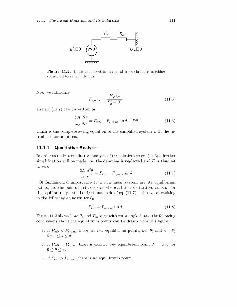
11.1. The Swing Equation and its Solutions 111
Xe
~Xd
′
UN 0∠Eq′ θ∠
Figure 11.2. Equivalent electric circuit of a synchronous machineconnected to an infinite bus.
Now we introduce
Pe,max =E′
qUN
X ′d + Xe
(11.5)
and eq. (11.2) can be written as
2H
ω0
d2θ
dt2= Pm0 − Pe,max sin θ − Dθ (11.6)
which is the complete swing equation of the simplified system with the in-troduced assumptions.
11.1.1 Qualitative Analysis
In order to make a qualitative analysis of the solutions to eq. (11.6) a furthersimplification will be made, i.e. the damping is neglected and D is thus setto zero :
2H
ω0
d2θ
dt2= Pm0 − Pe,max sin θ (11.7)
Of fundamental importance to a non-linear system are its equilibriumpoints, i.e. the points in state space where all time derivatives vanish. Forthe equilibrium points the right hand side of eq. (11.7) is thus zero resultingin the following equation for θ0
Pm0 = Pe,max sin θ0 (11.8)
Figure 11.3 shows how Pe and Pm vary with rotor angle θ, and the followingconclusions about the equilibrium points can be drawn from this figure:
1. If Pm0 < Pe,max there are two equilibrium points, i.e. θ0 and π − θ0
for 0 ≤ θ ≤ π.
2. If Pm0 = Pe,max there is exactly one equilibrium point θ0 = π/2 for0 ≤ θ ≤ π.
3. If Pm0 > Pe,max there is no equilibrium point.
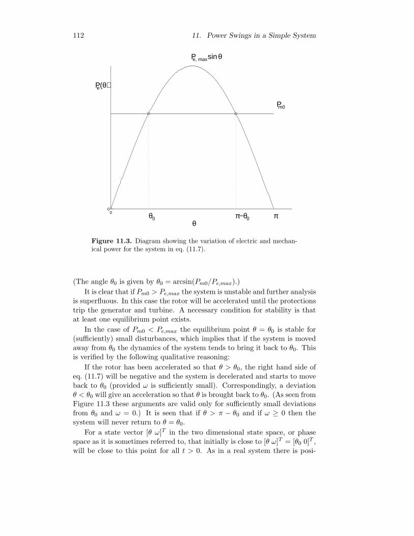
112 11. Power Swings in a Simple System
00
θ
P(θ)e
πθ0 π−θ0
Pe, maxsinθ
Pm0
Figure 11.3. Diagram showing the variation of electric and mechan-ical power for the system in eq. (11.7).
(The angle θ0 is given by θ0 = arcsin(Pm0/Pe,max).)
It is clear that if Pm0 > Pe,max the system is unstable and further analysisis superfluous. In this case the rotor will be accelerated until the protectionstrip the generator and turbine. A necessary condition for stability is thatat least one equilibrium point exists.
In the case of Pm0 < Pe,max the equilibrium point θ = θ0 is stable for(sufficiently) small disturbances, which implies that if the system is movedaway from θ0 the dynamics of the system tends to bring it back to θ0. Thisis verified by the following qualitative reasoning:
If the rotor has been accelerated so that θ > θ0, the right hand side ofeq. (11.7) will be negative and the system is decelerated and starts to moveback to θ0 (provided ω is sufficiently small). Correspondingly, a deviationθ < θ0 will give an acceleration so that θ is brought back to θ0. (As seen fromFigure 11.3 these arguments are valid only for sufficiently small deviationsfrom θ0 and ω = 0.) It is seen that if θ > π − θ0 and if ω ≥ 0 then thesystem will never return to θ = θ0.
For a state vector [θ ω]T in the two dimensional state space, or phasespace as it is sometimes referred to, that initially is close to [θ ω]T = [θ0 0]T ,will be close to this point for all t > 0. As in a real system there is posi-
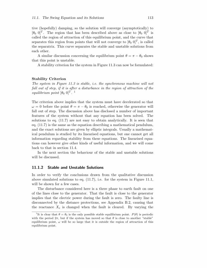
11.1. The Swing Equation and its Solutions 113
tive (hopefully) damping, so the solution will converge (asymptotically) to[θ0 0]T . The region that has been described above as close to [θ0 0]T iscalled the region of attraction of this equilibrium point, and the curve thatseparates this region from points that will not converge to [θ0 0]T , is calledthe separatrix. This curve separates the stable and unstable solutions fromeach other.
A similar discussion concerning the equilibrium point θ = π − θ0 showsthat this point is unstable.
A stability criterion for the system in Figure 11.3 can now be formulated:
Stability Criterion
The system in Figure 11.3 is stable, i.e. the synchronous machine will notfall out of step, if it is after a disturbance in the region of attraction of theequilibrium point [θ0 0]T . 1
The criterion above implies that the system must have decelerated so thatω = 0 before the point θ = π − θ0 is reached, otherwise the generator willfall out of step. The discussion above has disclosed a number of importantfeatures of the system without that any equation has been solved. Thesolutions to eq. (11.7) are not easy to obtain analytically. It is seen thateq. (11.7) is the same as the equation describing a mathematical pendulum,and the exact solutions are given by elliptic integrals. Usually a mathemat-ical pendulum is studied by its linearised equations, but one cannot get allinformation regarding stability from these equations. The linearised equa-tions can however give other kinds of useful information, and we will comeback to that in section 11.4.
In the next section the behaviour of the stable and unstable solutionswill be discussed.
11.1.2 Stable and Unstable Solutions
In order to verify the conclusions drawn from the qualitative discussionabove simulated solutions to eq. (11.7), i.e. for the system in Figure 11.1,will be shown for a few cases.
The disturbance considered here is a three phase to earth fault on oneof the lines close to the generator. That the fault is close to the generatorimplies that the electric power during the fault is zero. The faulty line isdisconnected by the distance protections, see Appendix B.2, causing thatthe reactance Xe is changed when the fault is cleared. By varying the
1It is clear that θ = θ0 is the only possible stable equilibrium point. P (θ) is periodicwith the period 2π, but if the system has moved so that θ is close to another “stable”equilibrium point, ω will be so large that it is outside the region of attraction of thisequilibrium point.
114 11. Power Swings in a Simple System
0 20 40 60 80 100 120 140 160 1800
0.2
0.4
0.6
0.8
1
1.2
1.4
1.6
1.8
2Electrical Power Before and After the Fault
Rotor Angle (degrees)
Ele
ctric
Pow
er (
p.u.
)
Figure 11.4. The electric power before the fault, Pe = 1.86 sin θ,after the fault, Pe = 1.26 sin θ, and the mechanical power, Pm = 1, asfunction of the rotor angle, θ.
fault clearing time different types of solutions to the swing equation can beobtained.
The system is thus described by the following equation
2H
ω0
d2θ
dt2= Pm0 − Pe,max sin θ − Dθ (11.9)
The electric power is as follows: Pre-fault Pe,max = 1.86 p.u., post faultPe,max = 1.26 p.u. and during the fault Pe = 0. Power curves before andafter fault are shown in Figure 11.4 where also the constant power from theturbine Pm = 1 p.u. is drawn. Before the fault θ = 32.5, which correspondsto the left intersection between Pe = 1.86 sin θ and Pm = 1. During the faultthe rotor will accelerate since Pe = 0 and consequently Pm − Pe > 0. Whenthe fault is cleared the electric power will follow the curve Pe = 1.24 sin θ.If the system is stable it will settle down to the point θ = 53.5 which isthe left intersection between Pe = 1.24 sin θ and Pm = 1. When the rotorangle is between 53.5 and 180 − 53.5 = 126.5, which corresponds to theright intersection between Pe = 1.24 sin θ and Pm = 1, then Pm − Pe < 0
11.1. The Swing Equation and its Solutions 115
and the rotor will decelerate. Should the rotor move beyond this point, thenPm −Pe > 0 and the rotor will accelerate and the system becomes unstable.It is often said that the generator falls out of step or loses synchronism.
The longer the duration of the fault, the more the rotor will be accel-erated and the larger the rotor angle. If the duration of the fault is toolong there is a risk that the rotor swing is so large that it passes the rightequilibrium point and the synchronous machine loses synchronism. To ver-ify and demonstrate this the system has been simulated for fault clearingtimes equal to 4, 6, 6.5, and 8 cycles.2 Results from these simulations areshown in Figures 11.5 to 11.8 where both the swing curves and the phaseportraits of the system are shown. The phase portrait, or phase trajectory,is the trajectory of the system in the (ω θ)-plane during the transient. Thedamping D is set to 0.02. The value of the damping determines how fasta stable solution will converge to its equilibrium point, and this value hasminor influence on the first swing directly after the fault.3
With a fault clearing time of 4 cycles the system is clearly stable, seeFigure 11.5. The maximal rotor angle is ≈ 90 which gives an ample marginto the critical value of 126.5. The system will eventually converge to thepoint θ = 53.5.
If the fault clearing time is increased to 6 cycles, see Figure 11.6, thestability margin is much smaller. The rotor swings out to ≈ 120 andit is very close to the critical point where it will start to accelerate. Ifthe fault clearing time is increased to 6.5 cycles the curves of Figure 11.7are obtained, and here the system is unstable. The generator cannot bedecelerated enough before it reaches the critical point, but it passes this pointand is further accelerated and loses synchronism. This type of instabilityis called first swing instability. The phase portrait in this case shows thatrotor is close to be decelerated before reaching the critical point, but it neverreaches a zero value of ω. The previous fault clearing time, i.e. 6 cycles, iscalled critical fault clearing time.
The last case shows a simulation with the fault clearing time equal to 8cycles, see Figure 11.8. In this case the rotor is accelerated for such a longtime that it passes the critical point very soon. The deceleration periodcould hardly be seen in the swing curve. The phase portrait shows also that
2Fault clearing times are often given in cycles of the power frequency. The reason forthis is that part of the clearing time comes from the time needed for the breakers to clearthe fault. Since the fault current can only be intercepted at a zero crossing, it is naturalto measure the breaker time in cycles. Modern high voltage breakers can break a faultcurrent in 2 – 3 cycles. Should still faster breaker times be required, special breakers couldbe installed, but these are more expensive than standard breakers. Protections are alsodescribed in Appendix B.
3This is the case for realistic values of D. If the damping is very large, and positive,this will increase the stability significantly in the system. The value used here is typicalin a system where no special equipment has been installed to increase the damping, e.g.Power System Stabilisers on the voltage regulators.
116 11. Power Swings in a Simple System
the deceleration just after fault clearing is clearly insufficient to stabilise thesystem.
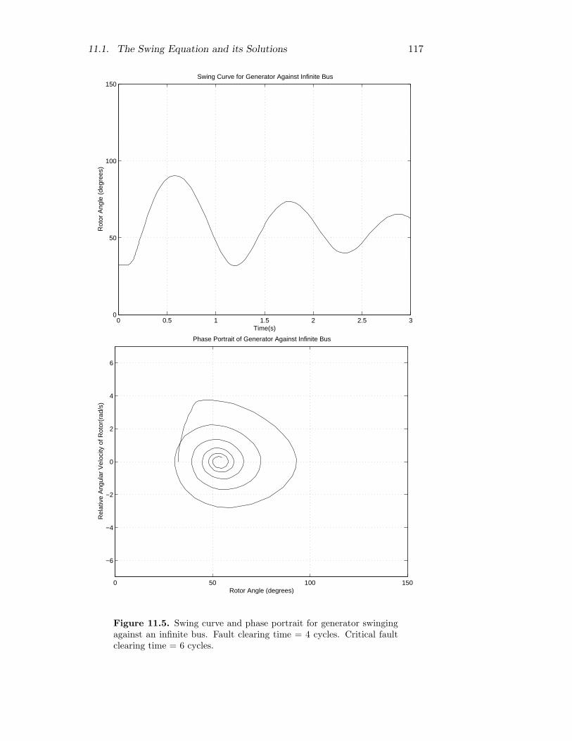
11.1. The Swing Equation and its Solutions 117
0 0.5 1 1.5 2 2.5 30
50
100
150
Time(s)
Rot
or A
ngle
(de
gree
s)
Swing Curve for Generator Against Infinite Bus
0 50 100 150
−6
−4
−2
0
2
4
6
Rotor Angle (degrees)
Rel
ativ
e A
ngul
ar V
eloc
ity o
f Rot
or(r
ad/s
)
Phase Portrait of Generator Against Infinite Bus
Figure 11.5. Swing curve and phase portrait for generator swingingagainst an infinite bus. Fault clearing time = 4 cycles. Critical faultclearing time = 6 cycles.
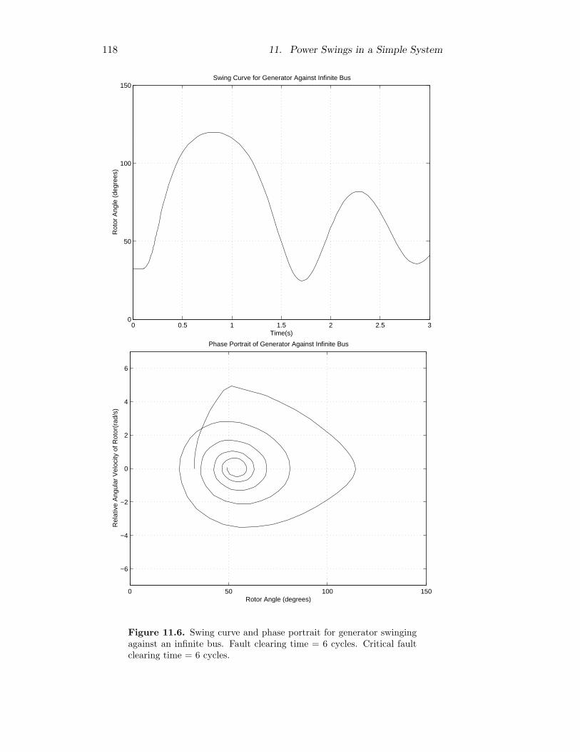
118 11. Power Swings in a Simple System
0 0.5 1 1.5 2 2.5 30
50
100
150
Time(s)
Rot
or A
ngle
(de
gree
s)
Swing Curve for Generator Against Infinite Bus
0 50 100 150
−6
−4
−2
0
2
4
6
Rotor Angle (degrees)
Rel
ativ
e A
ngul
ar V
eloc
ity o
f Rot
or(r
ad/s
)
Phase Portrait of Generator Against Infinite Bus
Figure 11.6. Swing curve and phase portrait for generator swingingagainst an infinite bus. Fault clearing time = 6 cycles. Critical faultclearing time = 6 cycles.
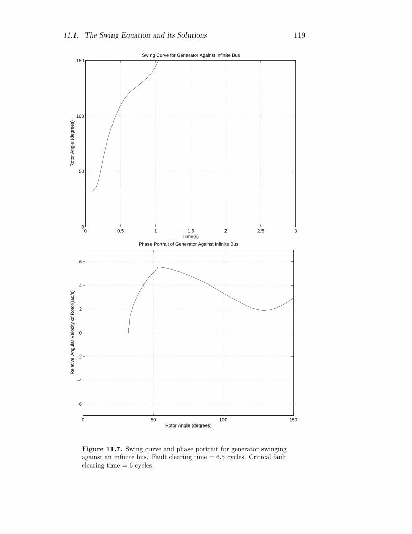
11.1. The Swing Equation and its Solutions 119
0 0.5 1 1.5 2 2.5 30
50
100
150
Time(s)
Rot
or A
ngle
(de
gree
s)
Swing Curve for Generator Against Infinite Bus
0 50 100 150
−6
−4
−2
0
2
4
6
Rotor Angle (degrees)
Rel
ativ
e A
ngul
ar V
eloc
ity o
f Rot
or(r
ad/s
)
Phase Portrait of Generator Against Infinite Bus
Figure 11.7. Swing curve and phase portrait for generator swingingagainst an infinite bus. Fault clearing time = 6.5 cycles. Critical faultclearing time = 6 cycles.
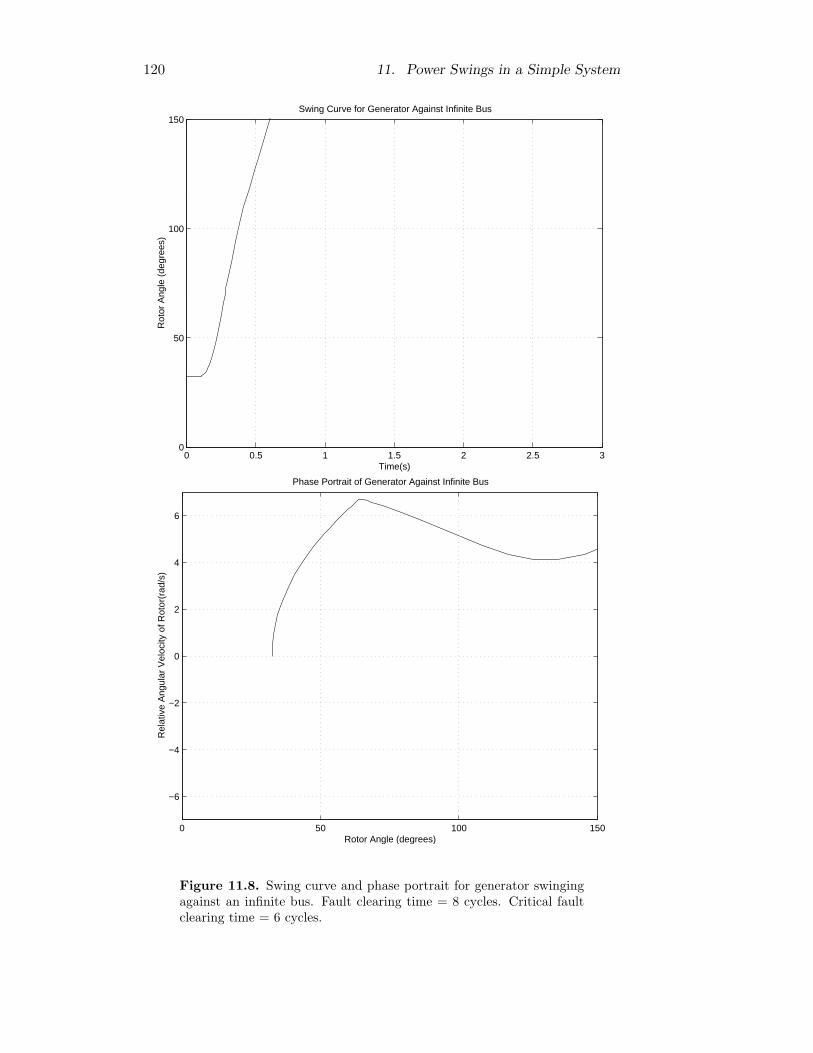
120 11. Power Swings in a Simple System
0 0.5 1 1.5 2 2.5 30
50
100
150
Time(s)
Rot
or A
ngle
(de
gree
s)
Swing Curve for Generator Against Infinite Bus
0 50 100 150
−6
−4
−2
0
2
4
6
Rotor Angle (degrees)
Rel
ativ
e A
ngul
ar V
eloc
ity o
f Rot
or(r
ad/s
)
Phase Portrait of Generator Against Infinite Bus
Figure 11.8. Swing curve and phase portrait for generator swingingagainst an infinite bus. Fault clearing time = 8 cycles. Critical faultclearing time = 6 cycles.
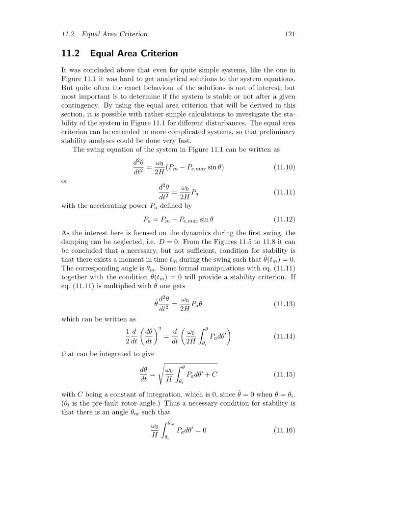
11.2. Equal Area Criterion 121
11.2 Equal Area Criterion
It was concluded above that even for quite simple systems, like the one inFigure 11.1 it was hard to get analytical solutions to the system equations.But quite often the exact behaviour of the solutions is not of interest, butmost important is to determine if the system is stable or not after a givencontingency. By using the equal area criterion that will be derived in thissection, it is possible with rather simple calculations to investigate the sta-bility of the system in Figure 11.1 for different disturbances. The equal areacriterion can be extended to more complicated systems, so that preliminarystability analyses could be done very fast.
The swing equation of the system in Figure 11.1 can be written as
d2θ
dt2=
ω0
2H(Pm − Pe,max sin θ) (11.10)
ord2θ
dt2=
ω0
2HPa (11.11)
with the accelerating power Pa defined by
Pa = Pm − Pe,max sin θ (11.12)
As the interest here is focused on the dynamics during the first swing, thedamping can be neglected, i.e. D = 0. From the Figures 11.5 to 11.8 it canbe concluded that a necessary, but not sufficient, condition for stability isthat there exists a moment in time tm during the swing such that θ(tm) = 0.The corresponding angle is θm. Some formal manipulations with eq. (11.11)together with the condition θ(tm) = 0 will provide a stability criterion. Ifeq. (11.11) is multiplied with θ one gets
θd2θ
dt2=
ω0
2HPaθ (11.13)
which can be written as
1
2
d
dt
(
dθ
dt
)2
=d
dt
(
ω0
2H
∫ θ
θi
Padθ′)
(11.14)
that can be integrated to give
dθ
dt=
√
ω0
H
∫ θ
θi
Padθ′ + C (11.15)
with C being a constant of integration, which is 0, since θ = 0 when θ = θi.(θi is the pre-fault rotor angle.) Thus a necessary condition for stability isthat there is an angle θm such that
ω0
H
∫ θm
θi
Padθ′ = 0 (11.16)
122 11. Power Swings in a Simple System
or∫ θm
θi
Padθ′ = 0 (11.17)
The stability criterion can thus be formulated as:
The system is stable if there exists an angle θm such that the area below theaccelerating power Pa in the θ–P (θ) diagram between θi and θm vanishes.
In most cases of practical interest the dynamics could be divided into twodifferent phases: A first phase when the rotor is accelerated, and a secondphase when it is decelerated. Assume that the rotor is accelerated up toθ = θc and that it is decelerated when θc ≤ θ ≤ θm. Then two differentareas in the θ–P (θ) plane can be defined as
Aa =
∫ θc
θi
(Pm − Pe(θ′))dθ′ (11.18)
Ar =
∫ θm
θc
(Pe(θ′) − Pm)dθ′ (11.19)
Indices a and r denote here accelerating and decelerating (retarding) areas,respectively. The angle θc is most conveniently chosen as the angle whenthe fault is cleared. The stability criterion can now be formulated as
The system is stable if there exists an angle θm such that the areas Aa andAr are equal, i.e. Aa = Ar.
This latter formulation gave rise to the name equal area criterion forthis stability criterion. This is illustrated in Figure 11.9. Note that Pe isreduced to zero during the fault, hence the shape of the area Aa.
The advantage of the equal area criterion is that the stability of a systemcan be investigated without any excessive computational efforts. But theprice paid is that the time t was eliminated from the equations. Since thetime does not appear explicitly in the equations, actions to improve thestability must be formulated in the angle space, which is usually not sopractical. It is of course of more interest to have these actions formulated interms of times, e.g. critical fault clearing times. By the equal area criterioncritical fault clearing angles could be formulated, and these must then betransformed to critical fault clearing times. Sometimes this can be doneeasily, sometimes it is not straightforward.
In the second formulation of the equal area criterion, an angle θc wasintroduced. This angle defines for which values that Pa should be calculatedas positive and negative, respectively. The choice of θc has no influence onthe result from the equal area criterion, which is obvious from the firstformulation. When applying the equal area criterion in a practical case it is
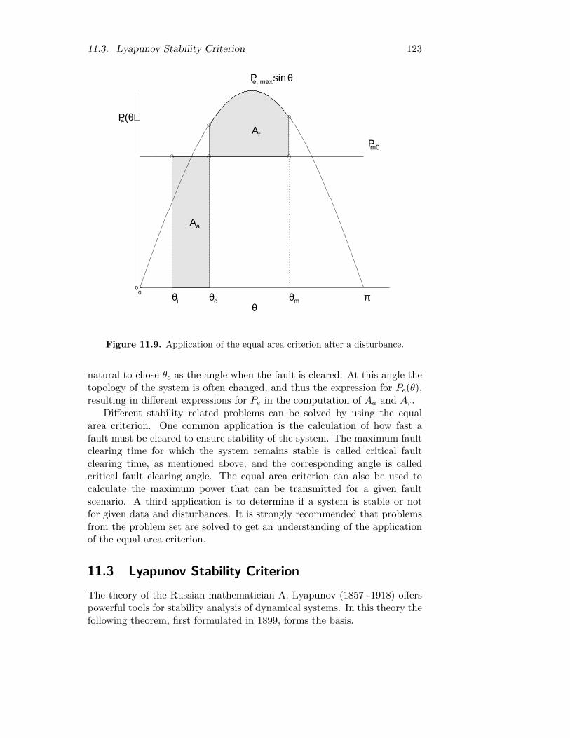
11.3. Lyapunov Stability Criterion 123
00
Aa
Ar
θ
P(θ)e
πθi θc θm
Pe, maxsinθ
Pm0
Figure 11.9. Application of the equal area criterion after a disturbance.
natural to chose θc as the angle when the fault is cleared. At this angle thetopology of the system is often changed, and thus the expression for Pe(θ),resulting in different expressions for Pe in the computation of Aa and Ar.
Different stability related problems can be solved by using the equalarea criterion. One common application is the calculation of how fast afault must be cleared to ensure stability of the system. The maximum faultclearing time for which the system remains stable is called critical faultclearing time, as mentioned above, and the corresponding angle is calledcritical fault clearing angle. The equal area criterion can also be used tocalculate the maximum power that can be transmitted for a given faultscenario. A third application is to determine if a system is stable or notfor given data and disturbances. It is strongly recommended that problemsfrom the problem set are solved to get an understanding of the applicationof the equal area criterion.
11.3 Lyapunov Stability Criterion
The theory of the Russian mathematician A. Lyapunov (1857 -1918) offerspowerful tools for stability analysis of dynamical systems. In this theory thefollowing theorem, first formulated in 1899, forms the basis.
124 11. Power Swings in a Simple System
Theorem. Consider the dynamical system x = f(x), where x0 is an equi-librium point. If in a region around the point x0 there exists a real valuedand continuously differentiable function V such that
1. V(x) > 0 and V(x0) = 0,
2. V(x) = grad(V(x)) · f(x) ≤ 0,
then x0 is a stable equilibrium point. If V(x) < 0, then x0 is asymptoticallystable.
The existence of the function V is also a necessary condition for stability.A problem with Lyapunov’s theorem is that it does not give any informa-tion on how to find the function V. It is obvious from the theorem thatV can be regarded as a form of energy, and the theorem says that if thesystem is stable, it will stay in the region around x = x0 where V is positivedefinite provided the “energy” introduced to the system by a disturbance issufficiently small.
For the system studied above the following function can be shown tofulfill the requirements of Lyapunov’s theorem
V(ω, θ) =H
ω0ω2 + Pm0(θ0 − θ) + Pe,max(cos θ0 − cos θ) = Vk + Vp (11.20)
with
Vk =H
ω0ω2 (11.21)
and
Vp = Pm0(θ0 − θ) + Pe,max(cos θ0 − cos θ) (11.22)
Vk can here be interpreted as kinetic energy and Vp as potential energy.
It is straightforward to show that V = −Dω2 by using eq. (11.6), andconsequently the second requirement of the above theorem is fulfilled if D ≥0. It is clear that V is positive definite in ω. In Figure 11.10 the potentialenergy, Vp is shown for a system with Pm0 = 0.3 and Pe,max = 1 and itcan be seen that it is positive definite in a neighbourhood of the equilibriumpoint θ0 = arcsin(Pm0/Pe,max). Thus, if the energy injected into the systemduring the fault will be less than the potential energy at the local maximumof Vp, the system will be stable. It can be shown that the above Lyapunovfunction, V, gives the same stability criterion as the equal area criterion.
11.4 Small Signal Analysis
The equal area criterion offers a tool to make stability analyses of the systemin Figure 11.1 by rather simple computations. For this system it is alsopossible to do other types of analyses that do not require any more extensive
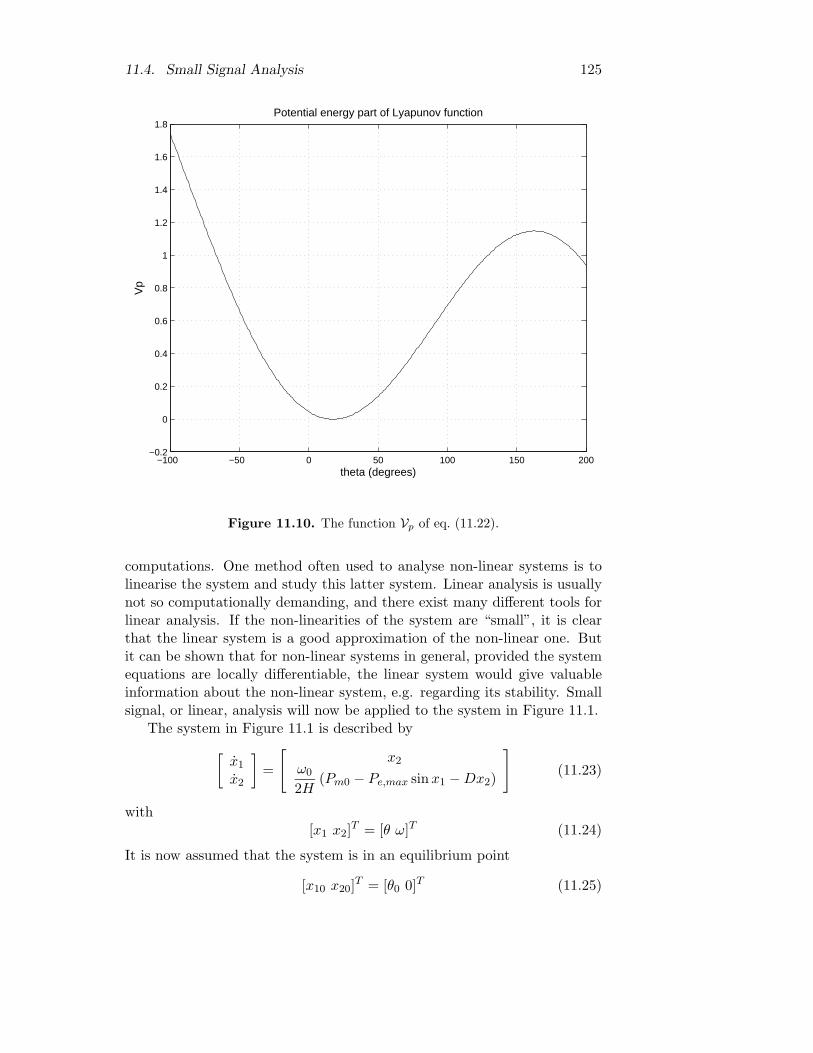
11.4. Small Signal Analysis 125
−100 −50 0 50 100 150 200−0.2
0
0.2
0.4
0.6
0.8
1
1.2
1.4
1.6
1.8
theta (degrees)
Vp
Potential energy part of Lyapunov function
Figure 11.10. The function Vp of eq. (11.22).
computations. One method often used to analyse non-linear systems is tolinearise the system and study this latter system. Linear analysis is usuallynot so computationally demanding, and there exist many different tools forlinear analysis. If the non-linearities of the system are “small”, it is clearthat the linear system is a good approximation of the non-linear one. Butit can be shown that for non-linear systems in general, provided the systemequations are locally differentiable, the linear system would give valuableinformation about the non-linear system, e.g. regarding its stability. Smallsignal, or linear, analysis will now be applied to the system in Figure 11.1.
The system in Figure 11.1 is described by
[
x1
x2
]
=
[
x2ω0
2H(Pm0 − Pe,max sin x1 − Dx2)
]
(11.23)
with[x1 x2]
T = [θ ω]T (11.24)
It is now assumed that the system is in an equilibrium point
[x10 x20]T = [θ0 0]T (11.25)
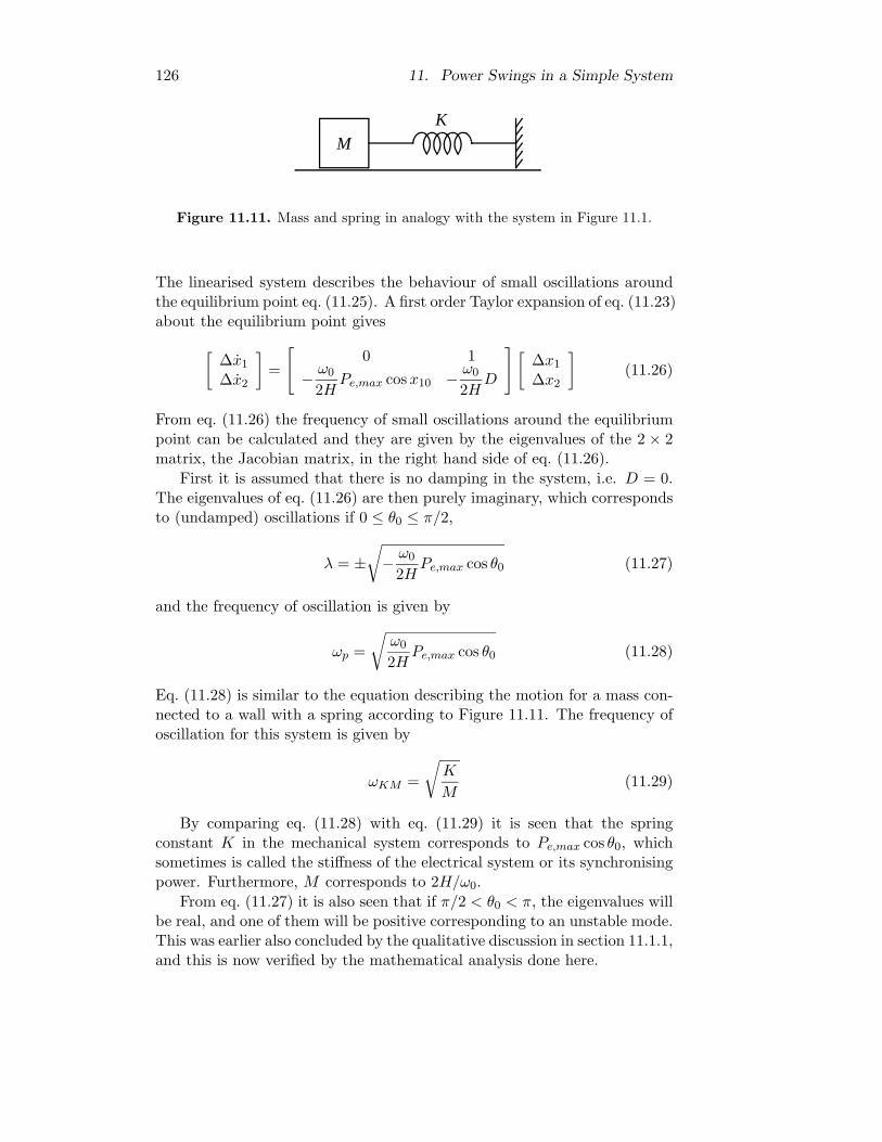
126 11. Power Swings in a Simple System
M
K
Figure 11.11. Mass and spring in analogy with the system in Figure 11.1.
The linearised system describes the behaviour of small oscillations aroundthe equilibrium point eq. (11.25). A first order Taylor expansion of eq. (11.23)about the equilibrium point gives
[
∆x1
∆x2
]
=
[
0 1
− ω0
2HPe,max cos x10 − ω0
2HD
]
[
∆x1
∆x2
]
(11.26)
From eq. (11.26) the frequency of small oscillations around the equilibriumpoint can be calculated and they are given by the eigenvalues of the 2 × 2matrix, the Jacobian matrix, in the right hand side of eq. (11.26).
First it is assumed that there is no damping in the system, i.e. D = 0.The eigenvalues of eq. (11.26) are then purely imaginary, which correspondsto (undamped) oscillations if 0 ≤ θ0 ≤ π/2,
λ = ±√
− ω0
2HPe,max cos θ0 (11.27)
and the frequency of oscillation is given by
ωp =
√
ω0
2HPe,max cos θ0 (11.28)
Eq. (11.28) is similar to the equation describing the motion for a mass con-nected to a wall with a spring according to Figure 11.11. The frequency ofoscillation for this system is given by
ωKM =
√
K
M(11.29)
By comparing eq. (11.28) with eq. (11.29) it is seen that the springconstant K in the mechanical system corresponds to Pe,max cos θ0, whichsometimes is called the stiffness of the electrical system or its synchronisingpower. Furthermore, M corresponds to 2H/ω0.
From eq. (11.27) it is also seen that if π/2 < θ0 < π, the eigenvalues willbe real, and one of them will be positive corresponding to an unstable mode.This was earlier also concluded by the qualitative discussion in section 11.1.1,and this is now verified by the mathematical analysis done here.
11.5. Methods to Improve System Stability 127
It was pointed out earlier that the damping is not significant for largedisturbances in the system. For large disturbances it is the ability of thesystem to stay within the region of attraction of the equilibrium point thatis important. This is depending on the stiffness of the system. The dampingis more important for how the system settles down to the equilibrium pointwhen it has survived the first swing. The linearised system could thus beused for studies of the damping in power systems. For the simple systemstudied here the eigenvalues with D 6= 0 become
λ = −D′
2± j
√
(ωp)2 −
(
D′
2
)2
(11.30)
with ωp given by eq. (11.28) and
D′ =ω0
2HD (11.31)
As the damping in a power system usually is quite small, eq. (11.30) can beapproximated by
λ ≈ −D′
2± jωp (11.32)
The frequency of oscillations can also be approximated in this case with goodaccuracy by eq. (11.28), and it is thus determined mainly by the stiffness ofthe system and the inertia constant of the machine.
11.5 Methods to Improve System Stability
It is obvious that it is desirable that a power system can withstand as manydisturbances as possible without becoming unstable. However, it is realisedthat it is not possible to design a system that can cope with all conceivablecontingencies, so one has to restrict the considered disturbances in the de-sign of the system. Usually, one considers only the most frequent faults inthe system. It is also important to consider the consequence of a fault ordisturbance when designing a system. Generally it can be said that the moreinvestments that can be made in a system, the more robust the system canbe made. One is thus faced with a technical-economical optimisation prob-lem that is very complex. Furthermore, there are a number of parametersthat are both very important in the optimisation process and at the sametime very hard to quantify. Such a parameter is the value that consumersput on uninterruptable supply of electric power of good quality. This opti-misation process has gained a lot of interest during the last few years due tothe liberalisation (de-regulation) of the power market taking place all overthe world. Theoretically the optimum value of reliability of power supply iswhen the marginal increase in the value perceived by the customers is equalto the cost of the investment made to achieve this increase in reliability.
128 11. Power Swings in a Simple System
Practically it is of course impossible to deduce this optimum, and one hasto judge by different methods if the consumers are satisfied with the relia-bility of the system, and if not if they are willing to pay more to improveit.
To have some more clear and practical rules for system design a numberof deterministic rules have been used over the years. One such rule is theso called (N − 1)-rule, which says that a system should be able to supplycustomer loads with any component, generator, line, etc., out of service.The disconnection of the component should preceded by a fault and thetransients triggered by this fault should be considered. A more conservativeapproach would be to apply an (N − 2)-criterion, which would result in amore reliable but more expensive system.
Modern methods apply probabilistic tools. In many of these approachesone considers both the probability of a fault and its consequences. By as-signing a measure, i.e. a number, for this combination of fault probabilityand consequence a risk based security analysis can be made. Some of theseaspects are also discussed in chapter 14.
This section will be concluded by a discussion of different ways to improvethe angular stability in power systems. The stabilising effect of the differentmethods can be verified by studying Figures 11.3 and 11.9. Which method toapply in a given situation depends on a large number of parameters and mustbe determined from case to case, usually after extensive studies. In somecases, one or several methods can be excluded, e.g. the construction of newlines since the needed permission cannot be granted from the authorities.The most common methods to increase system angular stability are:
• Increase of the inertia constant of the generators. This makes therotors more difficult to accelerate in connection with faults and therisk for losing synchronism is reduced. In most cases this is a veryexpensive means and only in special cases it can be applied, e.g. byinstalling a flywheel on a small hydro unit.
• Increase of system voltage. This increases Pe,max and for given powerPm the stability margin is increased.
• Reduction of the transfer reactance Xe. This will also increase Pe,max
as in the previous case. This can be achieved by constructing parallellines, or by installing series capacitors on existing lines or new lines.By installing series capacitors the effective reactance of the line isreduced. This method has been used extensively over the years, e.g.in the Swedish system.
• Installation of fast protections and fast breakers. In this way the timewith a fault connected can be reduced and thereby the time duringwhich the generator rotors are accelerated. The ability for the system
11.5. Methods to Improve System Stability 129
to decelerate the rotor swings is increased. Another way is to useautomatic re-closure after the fault is cleared, see Appendix A.
• Implementation of fast valving in steam turbines. By fast control ofthe mechanical power during and after a fault, the acceleration of therotors can be decreased. It cannot be applied to nuclear power plantsby security reasons. The method has not been used to any largerextent, since it is claimed to impose large thermal and mechanicalstresses on valves, turbines, etc.
• Installation of braking resistors. These are shunt resistors that areconnected by breakers fast after a fault close to a critical generator.The electric load of the critical machine increases and the risk forlosing synchronism is reduced.
• Stability control of controllable devices such as High Voltage DirectCurrent (HVDC), controllable series capacitors, controllable reactiveshunt compensation (SVC), etc. These devices are usually too ex-pensive to install just for stabilising the system, but when they areinstalled, the cost to use their controllability for stabilisation is usu-ally marginal.

130 11. Power Swings in a Simple System
12Oscillations in Multi-Machine Systems
This chapter contains a very brief overview of modelling of multi-machinepower systems. Many of the issues mentioned here will be dealt with in theadvanced course on power system analysis.
12.1 Simplified Model
The simplified model considered in the previous section has of course alimited application to realistic systems. The analysis of such a simple modelis primary motivated by the insight it gives, and by that the model can beused for simplified, preliminary calculations. In this section we will expandthe model to a system with more than one machine. The same assumptionsfor modelling are established, i.e.:
• The damping is neglected.
• The mechanical power is constant.
• The synchronous machines are modelled as constant voltage sourcesbehind the transient reactance. The phase angle for the voltage sourcecoincides with the rotor angle.
• Loads are represented by impedances (admittances).
A model based on these assumptions is usually referred to as the classicalmodel for electro-mechanical oscillations.
Since the loads are represented by impedances the load buses can be elim-inated and included in the node-admittance matrix, and the power whichflows out from the generators can be written as a function of the voltagemagnitudes and phase angles of the different machines.
Pei = Pei(E, θ) (12.1)
where E is a vector of voltages, of the N generators, and θ is a vector oftheir rotor angles
θ =[
θ1 θ2 . . . θN
]T(12.2)
131
132 12. Oscillations in Multi-Machine Systems
and analogously for E. The swing equation for machine i can now be writtenas
[
θi
ωi
]
=
[
ωiω0
2Hi(Pmi − Pei)
]
(12.3)
To get a compact form of this system of equations we introduce
x =[
θ1 ω1 . . . θN ωN
]T(12.4)
and the N coupled equations in (12.3) can be written as
x = f(x) (12.5)
where f is a vector valued function containing the swing equations for thedifferent machines. This system of swing equations is not easily analysed inthe general case. In most cases numerical methods must be used for studiesof the solutions. It can also be done by studying the linearised systemaccording to the method in section 11.4. It is found that the system canbe compared to a mechanical system with N masses connected with springsand with spring constants determined by the stiffnesses of the lines. Theeigenvalues and eigenvectors of the Jacobian matrix define the swing modesof the system, which often give a very good picture of how the real systembehaves in the case of disturbances. Actual oscillations in the system oftencan be approximated with good accuracy with linear combinations of theseswing modes. Another way to analyse the system is by solving the non-linearequations with numerical integration (time-simulations).
12.2 Detailed Model
A number of simplifications were earlier introduced to facilitate the analysisof the equations by utilising well-known mathematical methods. Unfortu-nately, the used model has some important shortcomings which makes it lessappropriate for more accurate studies of the dynamics of the power system.The most serious shortcomings are:
• The load model is too simple. A large part of the loads consists ofasynchronous machines and other drives and their characteristics donot follow that of an impedance at voltage oscillations. In principle,the loads consume as much power as the generators produce. Thereforeit is equally motivated to develop realistic load models as to makedetailed models of the synchronous machines.
• The dynamics of the synchronous machines is too simple. Here it isonly determined by two states, θi and ωi, while a realistic model needsmore states for a satisfactory description. Different fluxes in the syn-chronous machines will vary with time and different regulators, e.g. for
12.2. Detailed Model 133
voltage and frequency, will have influence on the process. Saturationphenomena in generators can also have influence.
• Modern controllable equipment like static compensators (SVC) andhigh-voltage direct current transmissions (HVDC), will in many caseshave a great influence on the stability of the system. Therefore theseshould be modelled in an adequate way.
The shortcomings originate essentially from a simplified modelling ofimportant components in the system. A more detailed description givesnaturally a better description, but the overview and handiness of the prob-lem are at the same time lost. More complicated models imply that morestate variables must be introduced. In the classical model every generatoris modelled by two states, θi and ωi, while a more detailed model demandsmore states. To model exciters, voltage regulators, and turbine regulations,more states also need to be introduced. Components like SVC and HVDC,with associated control equipment generally also require dynamic modelling,which imply that new state variables must be introduced. For more real-istic load models, the load buses cannot be eliminated, as was done in theclassical model. This implies that the equations for loads will formulate aconstraint that the state variables must fulfill. The above outlined generalmodel for electro-mechanical oscillations has the following properties, whichare worthwhile to comment on:
• It is differential-algebraic. The classical model resulted in a pure dif-ferential equation. Differential-algebraic systems are much more com-plicated to analyse than systems which can be modelled by a ”pure”system of differential equations.
• The system is non-linear.
• The system is non-time-invariant, i.e. the time occurs explicitly in theequations. This depends on events in the system, e.g. disturbancesand connections, but even on protective actions of different kind.
For realistic power systems the number of state variables is very large.As an example, the Nordic system contains hundreds of generators and thetotal number of states at simulations can be up to several thousands. Theused analysis methods are based either on the linearised system or on time-simulations of the complete model.

134 12. Oscillations in Multi-Machine Systems
13Voltage Stability
Voltage stability has been a limiting factor in many power systems during thelast years. Due to a gradual increase in load the reactive power balance canbe critical at peak load conditions. This chapter summarises the basic con-cepts and provides basic analyses for two simple test systems. A number ofstability indicators are introduced and applied to one of the test systems. Theimportance of load characteristics and load dynamics are demonstrated.
IN THE PREVIOUS chapters it was shown that an active power imbal-ance could give rise to rotor oscillations, which can cause instability if the
disturbances are large enough. If all generators in a system rotate with thesame electrical angular velocity (in average over a certain time period) thesystem is said to be synchronously stable. (Sometimes it is said to be inangle stability). This type of stability is strongly connected to the activepower balance in the system. As has been seen from the static analysis thereactive power and the voltage are strongly coupled to each other. As a ruleof thumb it can be said that if there is net production of reactive powerin a node, the voltage is high in the node, while a deficit of reactive powerimplies that the voltage is low. It could now be asked whether the interplaybetween Q and U can also cause instabilities similar to the angular insta-bility discussed earlier. It turns out that this is the case. The underlyingmechanisms for this voltage instability will be dealt with in this chaptertogether with some methods of analysis.
13.1 Mechanisms of Voltage Instability
In chapter 8 voltage instabilities were classified into slow and fast ones. Evenif the physical mechanism is the same, i.e. a lack of reactive power, thepower system contingencies and power system structures causing them aredifferent. The final break down, collapse, in the system could be quite fastalso in a slow voltage instability, and the actual instability can sometimesbe disguised, which makes this kind of instability troublesome to detect ina real system. Consequently it can be hard to get reliable indicators toactivate preventive actions if the time needed is available.
135
136 13. Voltage Stability
13.1.1 Long Term Voltage Instability
The time scale of the long term, or slow, voltage instability could be tensof seconds to hours. It develops from a gradual lack of reactive power at anode or in a part of the system. Even if the voltage stability phenomenon isclosely coupled to the reactive power balance the active power plays a veryimportant role indirectly. Many loads have an inductive power factor thatis not unity, and thus an increase in active power will cause an increase inreactive power consumption. Furthermore, the reactive losses in transmis-sion lines are proportional to the square of the active power transmitted, soheavily loaded lines will influence the reactive power balance significantly. Avery deceptive role is sometimes played by synchronous machines and othersources of reactive power. These devices can often supply more reactivepower than their steady state rating for a limited time, sometimes up toseveral minutes, and during this period of time the reactive power balanceand voltage could be kept at acceptable values. However, when protectionsin these devices act to avoid that the equipment is damaged, the reactivepower output is drastically reduced with a very fast voltage collapse as aresult.
The contributing factors to a slow voltage collapse are thus:
• Load increase
• Load recovery after faults
• Reactive losses in line due to high power transfer (This could be causedby line outages due to contingencies.)
• Loss of reactive supply (Capacitors, synchronous machines, etc.)
For the second bullet above, the control and dynamics of load tap-changers are very important. A voltage reduction in the high voltage systemwill propagate to the lower voltage levels. This will usually result in a re-duction of the load powers. However, load tap-changers on the transformerswill try to restore the voltage on the low voltage side and thereby increasingthe load power. This has in most cases a de-stabilising effect on the voltagestability.
13.1.2 Short Term Voltage Instability
For the short term, or fast, voltage instability the actual voltage collapsecomes very soon after the disturbance, just a few seconds or less. In theseinstabilities, loads or other devices with special reactive power characteristicsare often involved. Such loads are e.g. induction motors that just after faultconsume a lot of reactive power. Other loads that could be very detrimentalin this context are some types of power electronics based equipment. As an
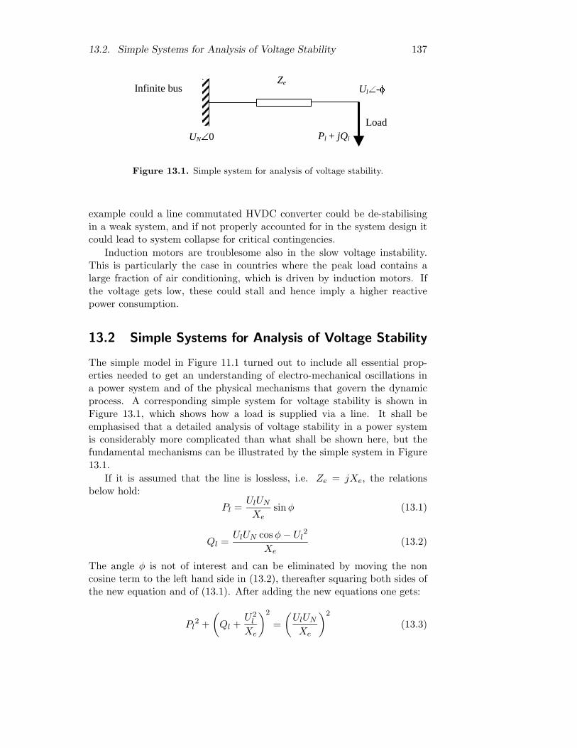
13.2. Simple Systems for Analysis of Voltage Stability 137
UlÐ-f
Pl + jQl
Load
Infinite bus
UNÐ0
Ze
Ð f
tÐ
Figure 13.1. Simple system for analysis of voltage stability.
example could a line commutated HVDC converter could be de-stabilisingin a weak system, and if not properly accounted for in the system design itcould lead to system collapse for critical contingencies.
Induction motors are troublesome also in the slow voltage instability.This is particularly the case in countries where the peak load contains alarge fraction of air conditioning, which is driven by induction motors. Ifthe voltage gets low, these could stall and hence imply a higher reactivepower consumption.
13.2 Simple Systems for Analysis of Voltage Stability
The simple model in Figure 11.1 turned out to include all essential prop-erties needed to get an understanding of electro-mechanical oscillations ina power system and of the physical mechanisms that govern the dynamicprocess. A corresponding simple system for voltage stability is shown inFigure 13.1, which shows how a load is supplied via a line. It shall beemphasised that a detailed analysis of voltage stability in a power systemis considerably more complicated than what shall be shown here, but thefundamental mechanisms can be illustrated by the simple system in Figure13.1.
If it is assumed that the line is lossless, i.e. Ze = jXe, the relationsbelow hold:
Pl =UlUN
Xesinφ (13.1)
Ql =UlUN cos φ − Ul
2
Xe(13.2)
The angle φ is not of interest and can be eliminated by moving the noncosine term to the left hand side in (13.2), thereafter squaring both sides ofthe new equation and of (13.1). After adding the new equations one gets:
Pl2 +
(
Ql +U2
l
Xe
)2
=
(
UlUN
Xe
)2
(13.3)
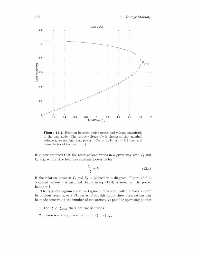
138 13. Voltage Stability
0 0.2 0.4 0.6 0.8 1 1.2 1.4 1.6 1.8 20
0.2
0.4
0.6
0.8
1
1.2Nose Curve
Load Power (Pl)
Load
Vol
tage
(U
l) Pl,max
Figure 13.2. Relation between active power and voltage magnitudein the load node. The source voltage UN is chosen so that nominalvoltage gives nominal load power. (UN = 1.044, Xe = 0.3 p.u., andpower factor of the load = 1.)
It is now assumed that the reactive load varies in a given way with Pl andUl, e.g. so that the load has constant power factor:
Ql
Pl= k (13.4)
If the relation between Pl and Ul is plotted in a diagram, Figure 13.2 isobtained, where it is assumed that k in eq. (13.4) is zero, i.e. the powerfactor = 1.
The type of diagram shown in Figure 13.2 is often called a “nose curve”by obvious reasons, or a PU-curve. From this figure three observations canbe made concerning the number of (theoretically) possible operating points:
1. For Pl < Pl,max there are two solutions.
2. There is exactly one solution for Pl = Pl,max.
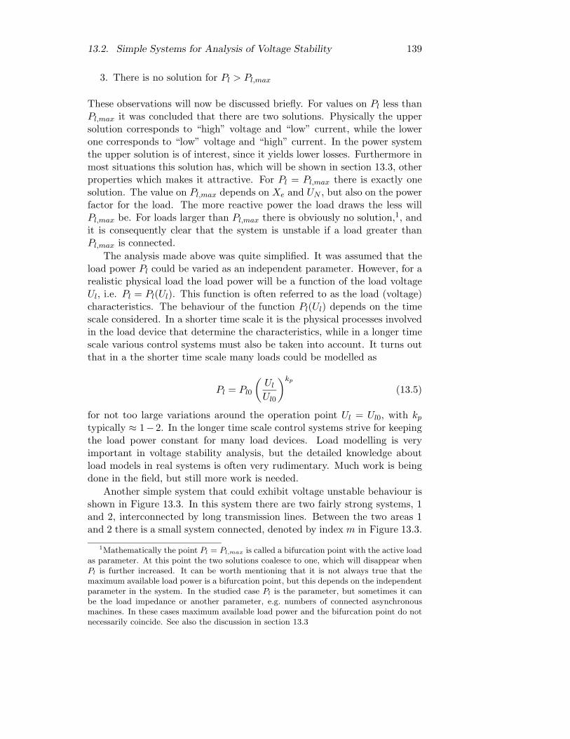
13.2. Simple Systems for Analysis of Voltage Stability 139
3. There is no solution for Pl > Pl,max
These observations will now be discussed briefly. For values on Pl less thanPl,max it was concluded that there are two solutions. Physically the uppersolution corresponds to “high” voltage and “low” current, while the lowerone corresponds to “low” voltage and “high” current. In the power systemthe upper solution is of interest, since it yields lower losses. Furthermore inmost situations this solution has, which will be shown in section 13.3, otherproperties which makes it attractive. For Pl = Pl,max there is exactly onesolution. The value on Pl,max depends on Xe and UN , but also on the powerfactor for the load. The more reactive power the load draws the less willPl,max be. For loads larger than Pl,max there is obviously no solution,1, andit is consequently clear that the system is unstable if a load greater thanPl,max is connected.
The analysis made above was quite simplified. It was assumed that theload power Pl could be varied as an independent parameter. However, for arealistic physical load the load power will be a function of the load voltageUl, i.e. Pl = Pl(Ul). This function is often referred to as the load (voltage)characteristics. The behaviour of the function Pl(Ul) depends on the timescale considered. In a shorter time scale it is the physical processes involvedin the load device that determine the characteristics, while in a longer timescale various control systems must also be taken into account. It turns outthat in a the shorter time scale many loads could be modelled as
Pl = Pl0
(
Ul
Ul0
)kp
(13.5)
for not too large variations around the operation point Ul = Ul0, with kp
typically ≈ 1− 2. In the longer time scale control systems strive for keepingthe load power constant for many load devices. Load modelling is veryimportant in voltage stability analysis, but the detailed knowledge aboutload models in real systems is often very rudimentary. Much work is beingdone in the field, but still more work is needed.
Another simple system that could exhibit voltage unstable behaviour isshown in Figure 13.3. In this system there are two fairly strong systems, 1and 2, interconnected by long transmission lines. Between the two areas 1and 2 there is a small system connected, denoted by index m in Figure 13.3.
1Mathematically the point Pl = Pl,max is called a bifurcation point with the active loadas parameter. At this point the two solutions coalesce to one, which will disappear whenPl is further increased. It can be worth mentioning that it is not always true that themaximum available load power is a bifurcation point, but this depends on the independentparameter in the system. In the studied case Pl is the parameter, but sometimes it canbe the load impedance or another parameter, e.g. numbers of connected asynchronousmachines. In these cases maximum available load power and the bifurcation point do notnecessarily coincide. See also the discussion in section 13.3
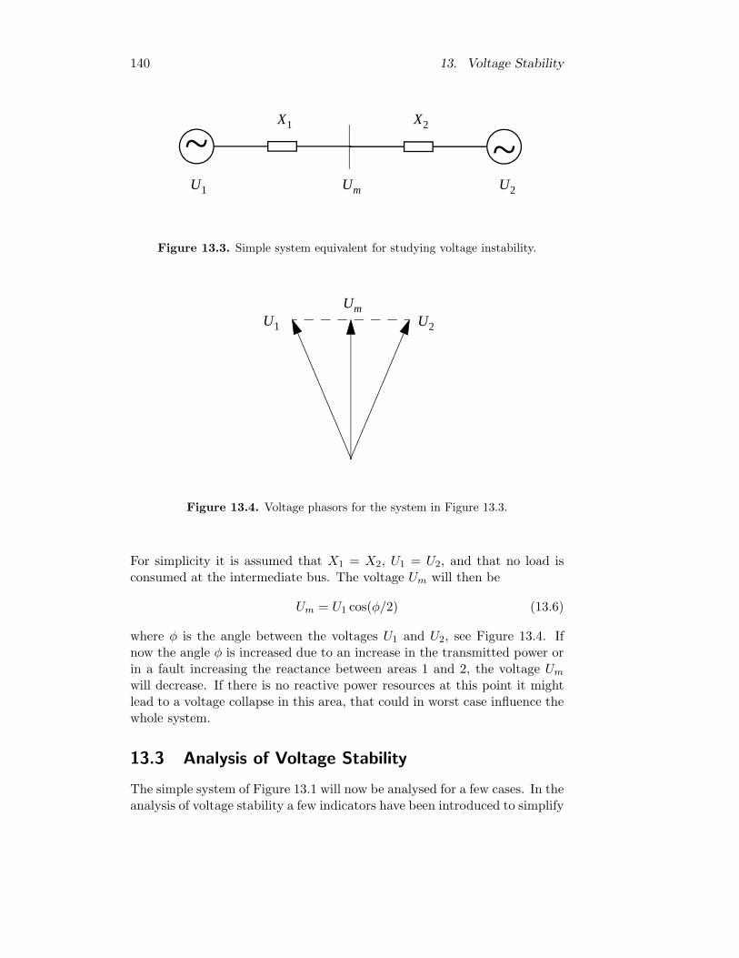
140 13. Voltage Stability
X1
~ ~X2
U1 U2Um
Figure 13.3. Simple system equivalent for studying voltage instability.
U1
UmU2
Figure 13.4. Voltage phasors for the system in Figure 13.3.
For simplicity it is assumed that X1 = X2, U1 = U2, and that no load isconsumed at the intermediate bus. The voltage Um will then be
Um = U1 cos(φ/2) (13.6)
where φ is the angle between the voltages U1 and U2, see Figure 13.4. Ifnow the angle φ is increased due to an increase in the transmitted power orin a fault increasing the reactance between areas 1 and 2, the voltage Um
will decrease. If there is no reactive power resources at this point it mightlead to a voltage collapse in this area, that could in worst case influence thewhole system.
13.3 Analysis of Voltage Stability
The simple system of Figure 13.1 will now be analysed for a few cases. In theanalysis of voltage stability a few indicators have been introduced to simplify
13.3. Analysis of Voltage Stability 141
the stability analysis. These indicators are based on small signal propertiesof the system and are consequently derived from linearised models. Asconcluded from the analysis of synchronous stability, linear analysis is oftenvery powerful, but must be used with care since it only captures the localbehaviour of the system around an operating point. To determine the globalbehaviour the full non-linear model must be employed.
13.3.1 Stability Indicators
In this section voltage stability indicators of the system in Figure 13.1 willbe discussed. Similar indicators with similar properties exist also for largersystems and these are often used in voltage stability studies of real systems.
Voltage Sensitivity Factor
The Voltage Sensitivity Factor VSF is one of the most used indicators orindices of voltage stability. It is defined for a given node i as
V SFi =∆Ui
∆Qi(13.7)
The physical interpretation of V SF is that it measures the change in voltagemagnitude at a given node as a consequence of a reactive power injectionin that node. Since all voltage control in a power system is based on that areactive power injection results in voltage increase, it is clear that a stabilitycriterion is
V SFi > 0 (13.8)
Furthermore, it is reasonable to require that an injection of reactive power inany node will not decrease the voltage in any node in the system. This prop-erty is often called voltage regularity. The V SF -indicator will be demon-strated on the system in Figure 13.1 later on.
∆U/∆E-indicator
Another indicator that is more closely related to the voltage control in apower system is given by ∆U/∆E, where U is the voltage magnitude of agiven bus and E is a voltage that is controllable, e.g. at the terminals of asynchronous machine. Also in this case the requirement of stability is givenby
∆U
∆E> 0 (13.9)
∆Qg/∆Ql-criterion
This criterion relates the reactive power consumed at the load(s) to thereactive power generated by the synchronous machines. In Figure 13.1 it
142 13. Voltage Stability
thus relates the reactive power injected at the infinite bus, here called Qg,to the reactive power consumed by the load Ql. The stability criterion is
∆Qg
∆Ql> 0 (13.10)
It can be shown that all the stability criteria above are equivalent inmost realistic systems. Which one to use is then dependent on which systemvariables that are known and controllable in a given situation. The threecriteria have also that in common that at the transition point to instabilitythey tend to infinity before going negative.
13.3.2 Analysis of Simple System
To gain a better understanding of the mechanisms governing voltage stabilitya few different cases will be analysed. The system in Figure 13.1 will be usedin all cases.
Influence of System Parameters
Here the influence of a few system parameters will be investigated. The nosecurve in Figure 13.2 was drawn for a lossless system, i.e. θ = 90, and thepower factor of the load being equal to unity. In Figure 13.5 the power factorhas been varied, and in Figure 13.6 nose curves for a number of differentvalues of the impedance angle is plotted. In all the cases the magnitude ofthe source voltage UN has been adjusted so that when the load is 1 p.u.the load voltage Ul = 1 p.u. From Figure 13.5 it can be concluded thatthe power factor has a significant influence on the nose curve, and therebyon the voltage stability. If the reactive consumption of the load could becompensated at the load point, this results in higher Pl,max but also in abetter voltage regulation around the nominal operating point.
The conclusion drawn from Figure 13.6 is that the impedance angle θdoes not influence the nose curve significantly for realistic values of highvoltage systems. A X/R ratio of 10 results in θ ≈ 84 and the deviationform the curve cooresponding to θ = 90 is insignificant. Thus, in thefollowing it will be assumed that θ = 90.
Influence of Load Characteristics
The voltage characteristics of the loads have a very large impact on thevoltage stability as will be shown in the following. It should be pointedout that the actual dynamics occurring in a real system during the courseof events to be discussed here could be very complicated and that the de-scription given here is simplified to emphasise the fundamental dynamics inthe system. The very detailed interplay between load dynamics and voltagecontrol might cause that the actual course of events turn out to be different.
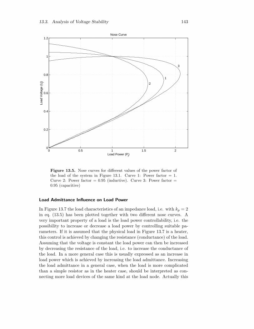
13.3. Analysis of Voltage Stability 143
0 0.5 1 1.5 20
0.2
0.4
0.6
0.8
1
1.2Nose Curve
Load Power (Pl)
Load
Vol
tage
(U
l)
1
2
3
Figure 13.5. Nose curves for different values of the power factor ofthe load of the system in Figure 13.1. Curve 1: Power factor = 1.Curve 2: Power factor = 0.95 (inductive). Curve 3: Power factor =0.95 (capacitive)
Load Admittance Influence on Load Power
In Figure 13.7 the load characteristics of an impedance load, i.e. with kp = 2in eq. (13.5) has been plotted together with two different nose curves. Avery important property of a load is the load power controllability, i.e. thepossibility to increase or decrease a load power by controlling suitable pa-rameters. If it is assumed that the physical load in Figure 13.7 is a heater,this control is achieved by changing the resistance (conductance) of the load.Assuming that the voltage is constant the load power can then be increasedby decreasing the resistance of the load, i.e. to increase the conductance ofthe load. In a more general case this is usually expressed as an increase inload power which is achieved by increasing the load admittance. Increasingthe load admittance in a general case, when the load is more complicatedthan a simple resistor as in the heater case, should be interpreted as con-necting more load devices of the same kind at the load node. Actually this
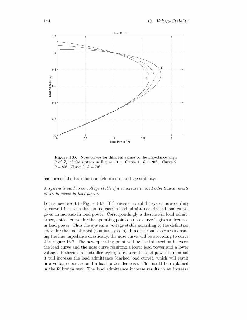
144 13. Voltage Stability
0 0.5 1 1.5 20
0.2
0.4
0.6
0.8
1
1.2Nose Curve
Load Power (Pl)
Load
Vol
tage
(U
l)
1
23
Figure 13.6. Nose curves for different values of the impedance angleθ of Ze of the system in Figure 13.1. Curve 1: θ = 90. Curve 2:θ = 80. Curve 3: θ = 70
has formed the basis for one definition of voltage stability:
A system is said to be voltage stable if an increase in load admittance resultsin an increase in load power.
Let us now revert to Figure 13.7. If the nose curve of the system is accordingto curve 1 it is seen that an increase in load admittance, dashed load curve,gives an increase in load power. Correspondingly a decrease in load admit-tance, dotted curve, for the operating point on nose curve 1, gives a decreasein load power. Thus the system is voltage stable according to the definitionabove for the undisturbed (nominal system). If a disturbance occurs increas-ing the line impedance drastically, the nose curve will be according to curve2 in Figure 13.7. The new operating point will be the intersection betweenthe load curve and the nose curve resulting a lower load power and a lowervoltage. If there is a controller trying to restore the load power to nominalit will increase the load admittance (dashed load curve), which will resultin a voltage decrease and a load power decrease. This could be explainedin the following way. The load admittance increase results in an increase
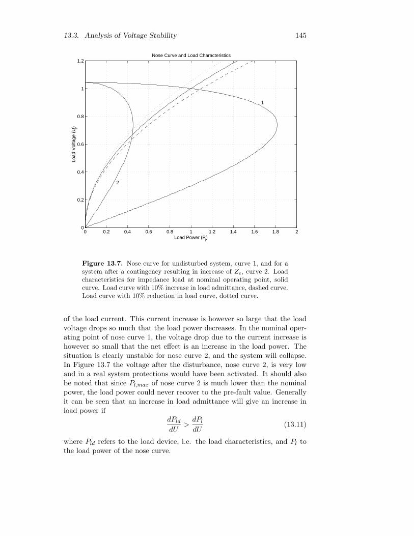
13.3. Analysis of Voltage Stability 145
0 0.2 0.4 0.6 0.8 1 1.2 1.4 1.6 1.8 20
0.2
0.4
0.6
0.8
1
1.2Nose Curve and Load Characteristics
Load Power (Pl)
Load
Vol
tage
(U
l)
1
2
Figure 13.7. Nose curve for undisturbed system, curve 1, and for asystem after a contingency resulting in increase of Ze, curve 2. Loadcharacteristics for impedance load at nominal operating point, solidcurve. Load curve with 10% increase in load admittance, dashed curve.Load curve with 10% reduction in load curve, dotted curve.
of the load current. This current increase is however so large that the loadvoltage drops so much that the load power decreases. In the nominal oper-ating point of nose curve 1, the voltage drop due to the current increase ishowever so small that the net effect is an increase in the load power. Thesituation is clearly unstable for nose curve 2, and the system will collapse.In Figure 13.7 the voltage after the disturbance, nose curve 2, is very lowand in a real system protections would have been activated. It should alsobe noted that since Pl,max of nose curve 2 is much lower than the nominalpower, the load power could never recover to the pre-fault value. Generallyit can be seen that an increase in load admittance will give an increase inload power if
dPld
dU>
dPl
dU(13.11)
where Pld refers to the load device, i.e. the load characteristics, and Pl tothe load power of the nose curve.
146 13. Voltage Stability
VSF Criterion
The V SF criterion was introduced above and that will now be analysedfor different load characteristics. This criterion is closely related to howthe voltage control will act in the system. It is rather straightforward tocalculate V SF for different load characteristics and operating points on thenose curve. From such an analysis the following can be concluded:
• For constant power loads, i.e. kp = 0 in eq. (13.5), operating pointson the upper half of the nose curve are stable, i.e. V SF > 0, whilethose on the lower part are unstable or V SF < 0.
• For impedance loads V SF > 0 for all operating points, indicatingvoltage regularity.
• For 0 < kp < 2 operating points on the upper part of the nose curveare stable. In addition a part of the lower part is also stable rangingfrom Pl,max to lower Pl values. This interval increases with kp withboundaries according to the two previous conclusions.
Since in a longer time scale most loads could be approximated by con-stant power loads, permanent operation is feasible only at the upper partof the nose curve. During transients operation on the lower part could beacceptable.
Load Dynamics
The discussion in this paragraph relates to the discussion concerning loadadmittance, but deals with a somewhat different disturbance. The systemin Figure 13.1 is considered again. It is now assumed that a voltage increaseof 5% occurs in the sending end system, i.e. UN is increased by 5%. InFigure 13.8 the nose curves and load characteristics corresponding to animpedance load are depicted. The load is controlled in such a way that theload power should be constant, which e.g. could be the case for a thermostatcontrolled heater. The voltage increase resulted in a load power increase andconsequently the load power control orders a decrease in load admittance.This decrease in load admittance results in the dashed load characteristicsin Figure 13.8, and the system can settle to a new operating point at thedesired load power, i.e. 1 p.u., but at a slightly higher voltage. An analysisof the behaviour of the system shows that, if the sending end voltage isslightly decreased, the system will settle at 1 p.u. load power at a slightlylower voltage.
Now assume that the system is operating on the lower part of the nosecurve, see Figure 13.9. According to the V SF criterion this operating pointis stable. The same disturbance as in the previous case is considered. FromFigures 13.8 and 13.9 it can be concluded that both systems are stable
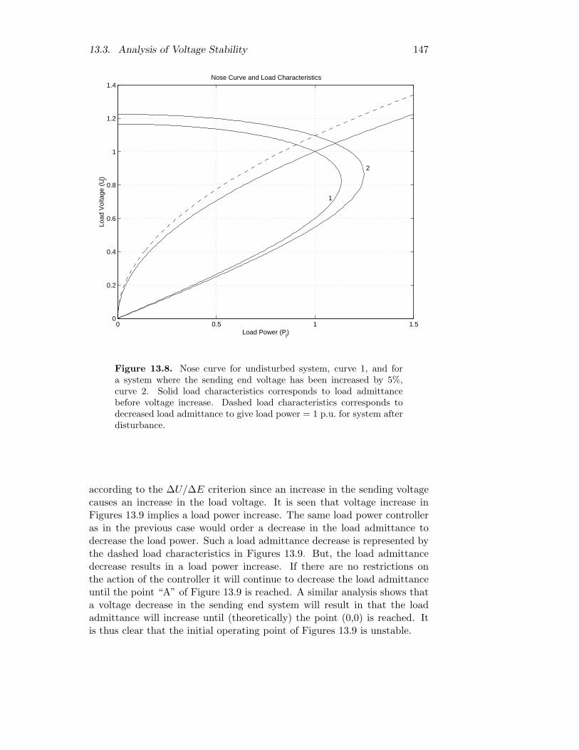
13.3. Analysis of Voltage Stability 147
0 0.5 1 1.50
0.2
0.4
0.6
0.8
1
1.2
1.4Nose Curve and Load Characteristics
Load Power (Pl)
Load
Vol
tage
(U
l)
1
2
Figure 13.8. Nose curve for undisturbed system, curve 1, and fora system where the sending end voltage has been increased by 5%,curve 2. Solid load characteristics corresponds to load admittancebefore voltage increase. Dashed load characteristics corresponds todecreased load admittance to give load power = 1 p.u. for system afterdisturbance.
according to the ∆U/∆E criterion since an increase in the sending voltagecauses an increase in the load voltage. It is seen that voltage increase inFigures 13.9 implies a load power increase. The same load power controlleras in the previous case would order a decrease in the load admittance todecrease the load power. Such a load admittance decrease is represented bythe dashed load characteristics in Figures 13.9. But, the load admittancedecrease results in a load power increase. If there are no restrictions onthe action of the controller it will continue to decrease the load admittanceuntil the point “A” of Figure 13.9 is reached. A similar analysis shows thata voltage decrease in the sending end system will result in that the loadadmittance will increase until (theoretically) the point (0,0) is reached. Itis thus clear that the initial operating point of Figures 13.9 is unstable.
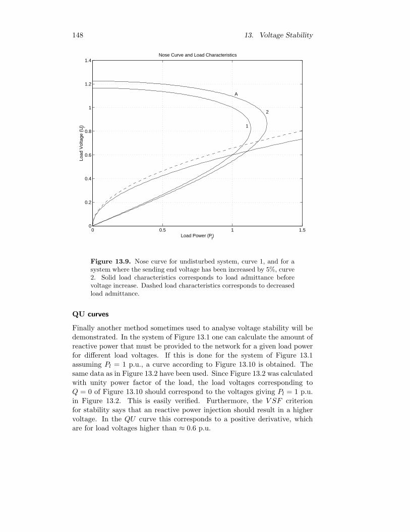
148 13. Voltage Stability
0 0.5 1 1.50
0.2
0.4
0.6
0.8
1
1.2
1.4Nose Curve and Load Characteristics
Load Power (Pl)
Load
Vol
tage
(U
l) 1
2
A
Figure 13.9. Nose curve for undisturbed system, curve 1, and for asystem where the sending end voltage has been increased by 5%, curve2. Solid load characteristics corresponds to load admittance beforevoltage increase. Dashed load characteristics corresponds to decreasedload admittance.
QU curves
Finally another method sometimes used to analyse voltage stability will bedemonstrated. In the system of Figure 13.1 one can calculate the amount ofreactive power that must be provided to the network for a given load powerfor different load voltages. If this is done for the system of Figure 13.1assuming Pl = 1 p.u., a curve according to Figure 13.10 is obtained. Thesame data as in Figure 13.2 have been used. Since Figure 13.2 was calculatedwith unity power factor of the load, the load voltages corresponding toQ = 0 of Figure 13.10 should correspond to the voltages giving Pl = 1 p.u.in Figure 13.2. This is easily verified. Furthermore, the V SF criterionfor stability says that an reactive power injection should result in a highervoltage. In the QU curve this corresponds to a positive derivative, whichare for load voltages higher than ≈ 0.6 p.u.
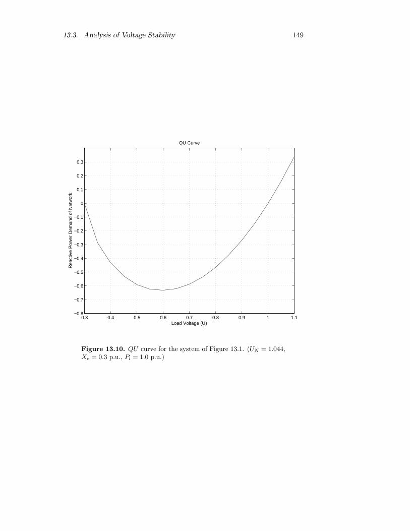
13.3. Analysis of Voltage Stability 149
0.3 0.4 0.5 0.6 0.7 0.8 0.9 1 1.1−0.8
−0.7
−0.6
−0.5
−0.4
−0.3
−0.2
−0.1
0
0.1
0.2
0.3
QU Curve
Rea
ctiv
e P
ower
Dem
and
of N
etw
ork
Load Voltage (Ul)
Figure 13.10. QU curve for the system of Figure 13.1. (UN = 1.044,Xe = 0.3 p.u., Pl = 1.0 p.u.)

150 13. Voltage Stability
14Control of Electric Power Systems
This chapter gives an introduction to control of power systems. Both thefaster distributed controls and slower centralised controls are described.
A POWER SYSTEM is planned, designed and built to supply the con-sumers with electrical energy considering:
• Economy
• Quality
• Supply security (Reliability)
• Environmental impact
The last point has become more and more important during the latestyears. This can be seen from the fact that most of the larger companiesnowadays have special departments responsible for that the companies fol-low laws and regulations within the environment area. The three first pointsabove constitute the basis of the optimisation that the power companiesmust make regarding their investments and daily operation. It is evidentthat economical considerations must be regarded when deciding issues aboutquality and supply security for the system. The higher quality and supplysecurity that is required, the more expensive the electrical energy becomes.Methods based on mathematical analysis and decision making theory (oper-ations research) have been worked out to handle this optimisation problem,which contains several considerations/adjustments that are hard to formu-late in a stringent mathematical form. As cheap and safe access to electricalenergy is of great importance for almost all activities in a modern society,it is not surprising that the decisions makers in the power industry werepioneers to utilise advanced optimisation methods and other analysis toolsfor expansion and investment planning.
In this compendium we will limit ourselves to discussing how a powersystem can be controlled to fulfill the constrains regarding quality. A veryshort introduction is also given about the overall control in a power system,which besides its aim to fulfill the quality even plays an important role inthe supply security.
151
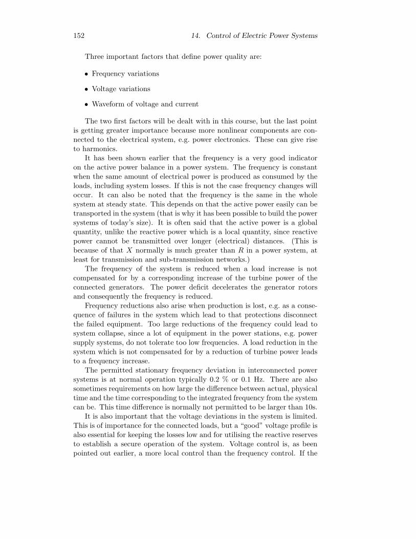
152 14. Control of Electric Power Systems
Three important factors that define power quality are:
• Frequency variations
• Voltage variations
• Waveform of voltage and current
The two first factors will be dealt with in this course, but the last pointis getting greater importance because more nonlinear components are con-nected to the electrical system, e.g. power electronics. These can give riseto harmonics.
It has been shown earlier that the frequency is a very good indicatoron the active power balance in a power system. The frequency is constantwhen the same amount of electrical power is produced as consumed by theloads, including system losses. If this is not the case frequency changes willoccur. It can also be noted that the frequency is the same in the wholesystem at steady state. This depends on that the active power easily can betransported in the system (that is why it has been possible to build the powersystems of today’s size). It is often said that the active power is a globalquantity, unlike the reactive power which is a local quantity, since reactivepower cannot be transmitted over longer (electrical) distances. (This isbecause of that X normally is much greater than R in a power system, atleast for transmission and sub-transmission networks.)
The frequency of the system is reduced when a load increase is notcompensated for by a corresponding increase of the turbine power of theconnected generators. The power deficit decelerates the generator rotorsand consequently the frequency is reduced.
Frequency reductions also arise when production is lost, e.g. as a conse-quence of failures in the system which lead to that protections disconnectthe failed equipment. Too large reductions of the frequency could lead tosystem collapse, since a lot of equipment in the power stations, e.g. powersupply systems, do not tolerate too low frequencies. A load reduction in thesystem which is not compensated for by a reduction of turbine power leadsto a frequency increase.
The permitted stationary frequency deviation in interconnected powersystems is at normal operation typically 0.2 % or 0.1 Hz. There are alsosometimes requirements on how large the difference between actual, physicaltime and the time corresponding to the integrated frequency from the systemcan be. This time difference is normally not permitted to be larger than 10s.
It is also important that the voltage deviations in the system is limited.This is of importance for the connected loads, but a “good” voltage profile isalso essential for keeping the losses low and for utilising the reactive reservesto establish a secure operation of the system. Voltage control is, as beenpointed out earlier, a more local control than the frequency control. If the
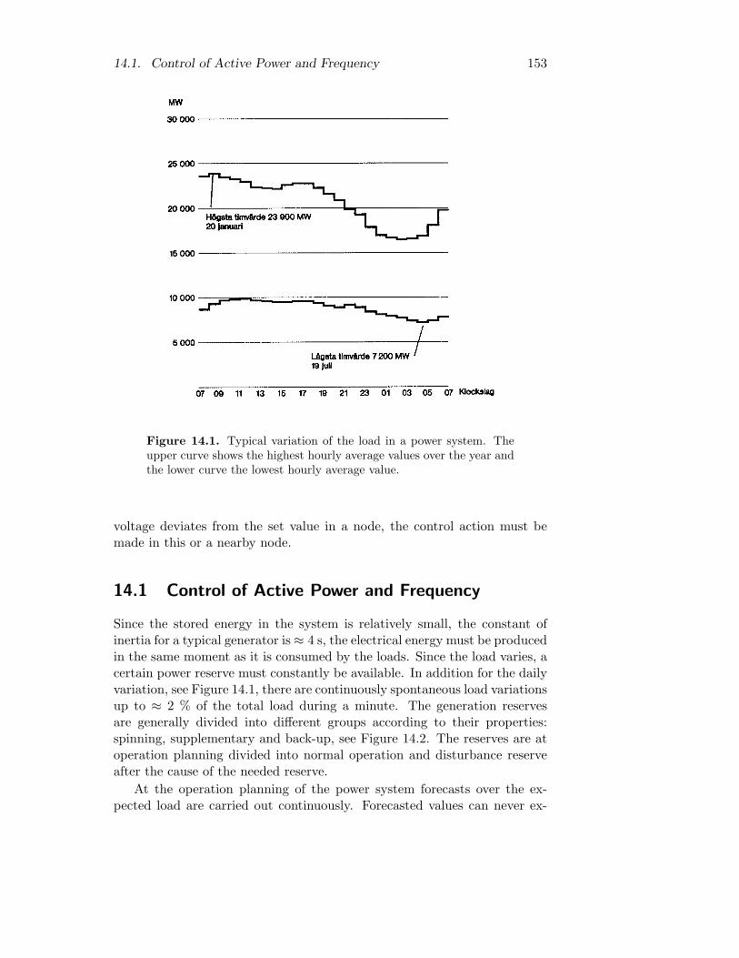
14.1. Control of Active Power and Frequency 153
Figure 14.1. Typical variation of the load in a power system. Theupper curve shows the highest hourly average values over the year andthe lower curve the lowest hourly average value.
voltage deviates from the set value in a node, the control action must bemade in this or a nearby node.
14.1 Control of Active Power and Frequency
Since the stored energy in the system is relatively small, the constant ofinertia for a typical generator is ≈ 4 s, the electrical energy must be producedin the same moment as it is consumed by the loads. Since the load varies, acertain power reserve must constantly be available. In addition for the dailyvariation, see Figure 14.1, there are continuously spontaneous load variationsup to ≈ 2 % of the total load during a minute. The generation reservesare generally divided into different groups according to their properties:spinning, supplementary and back-up, see Figure 14.2. The reserves are atoperation planning divided into normal operation and disturbance reserveafter the cause of the needed reserve.
At the operation planning of the power system forecasts over the ex-pected load are carried out continuously. Forecasted values can never ex-
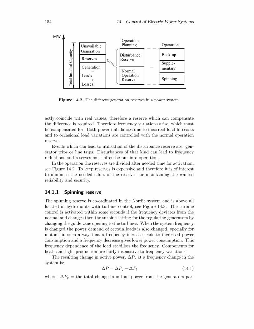
154 14. Control of Electric Power Systems
Unavailable
Reserves
Generation=
Loads+
LossesTo
tal
Inst
alle
d C
apac
ity
=
Operation
Back-up
Supple-
Spinning
NormalOperationReserve
DisturbanceReserve
OperationPlanning
MW
Generation
mentary
Figure 14.2. The different generation reserves in a power system.
actly coincide with real values, therefore a reserve which can compensatethe difference is required. Therefore frequency variations arise, which mustbe compensated for. Both power imbalances due to incorrect load forecastsand to occasional load variations are controlled with the normal operationreserve.
Events which can lead to utilisation of the disturbance reserve are: gen-erator trips or line trips. Disturbances of that kind can lead to frequencyreductions and reserves must often be put into operation.
In the operation the reserves are divided after needed time for activation,see Figure 14.2. To keep reserves is expensive and therefore it is of interestto minimise the needed effort of the reserves for maintaining the wantedreliability and security.
14.1.1 Spinning reserve
The spinning reserve is co-ordinated in the Nordic system and is above alllocated in hydro units with turbine control, see Figure 14.3. The turbinecontrol is activated within some seconds if the frequency deviates from thenormal and changes then the turbine setting for the regulating generators bychanging the guide vane opening to the turbines. When the system frequencyis changed the power demand of certain loads is also changed, specially formotors, in such a way that a frequency increase leads to increased powerconsumption and a frequency decrease gives lower power consumption. Thisfrequency dependence of the load stabilises the frequency. Components forheat- and light production are fairly insensitive to frequency variations.
The resulting change in active power, ∆P , at a frequency change in thesystem is:
∆P = ∆Pg − ∆Pl (14.1)
where: ∆Pg = the total change in output power from the generators par-
14.1. Control of Active Power and Frequency 155
Power System
∆Pmech ∆f f
fset
Uset
Ugen
Ufield
∆Uf
Turbine ~Pmech
Figure 14.3. Generator unit with voltage regulator and turbine reg-ulator for frequency control.
ticipating in the frequency control, ∆Pl = the total frequency dependentload power change. The frequency dependence of the load can often beapproximated as
∆Pl = D∆f (14.2)
where D is a constant. The value on D is typically 0 − 4 %/Hz, but largevariations occur depending on the kind of load.
The frequency control is performed so that, at least for small frequencydeviations, the total change in output power of the frequency controllinggenerators are (in steady state) proportional to the frequency change, ∆f .The relation between changes in active power and frequency deviations canthen be written
∆Pg = −R∆f (14.3)
The constant R is determined by the setting of the turbine control of thefrequency controlling generators, and is named the systems frequency regu-lation constant or frequency droop and is normally given in MW/Hz. Thefrequency regulation for a system is established so that the frequency doesnot fall outside given limits at certain dimensional disturbances which canoccur, e.g. trip of the largest generator in the system.
It shall be noted that the variation of frequency, computed from theabove relations, are the steady state values which are obtained after thefrequency controllers have responded. The transient frequency deviationduring the process following a large disturbance can be considerably largerthan the stationary one, up to some Hz. In Figure 14.4 it is shown howthe frequency can vary after a disturbance in the system. As seen themaximal frequency deviation is considerably greater than the stationary
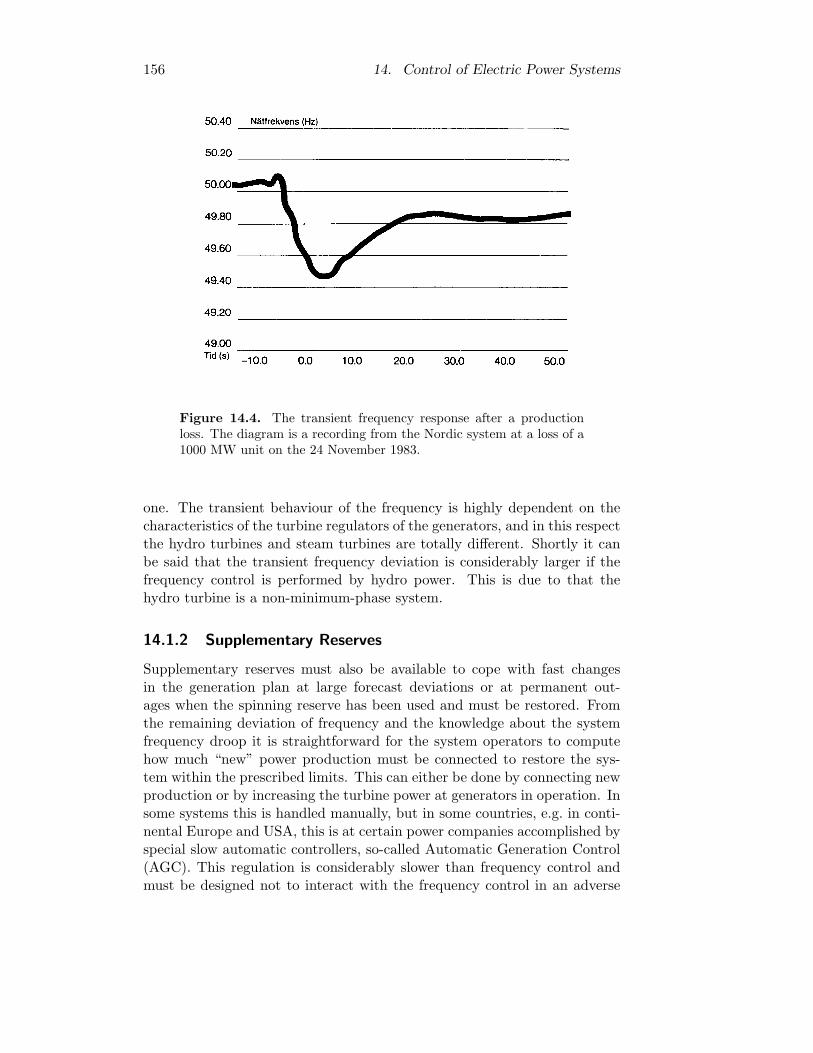
156 14. Control of Electric Power Systems
Figure 14.4. The transient frequency response after a productionloss. The diagram is a recording from the Nordic system at a loss of a1000 MW unit on the 24 November 1983.
one. The transient behaviour of the frequency is highly dependent on thecharacteristics of the turbine regulators of the generators, and in this respectthe hydro turbines and steam turbines are totally different. Shortly it canbe said that the transient frequency deviation is considerably larger if thefrequency control is performed by hydro power. This is due to that thehydro turbine is a non-minimum-phase system.
14.1.2 Supplementary Reserves
Supplementary reserves must also be available to cope with fast changesin the generation plan at large forecast deviations or at permanent out-ages when the spinning reserve has been used and must be restored. Fromthe remaining deviation of frequency and the knowledge about the systemfrequency droop it is straightforward for the system operators to computehow much “new” power production must be connected to restore the sys-tem within the prescribed limits. This can either be done by connecting newproduction or by increasing the turbine power at generators in operation. Insome systems this is handled manually, but in some countries, e.g. in conti-nental Europe and USA, this is at certain power companies accomplished byspecial slow automatic controllers, so-called Automatic Generation Control(AGC). This regulation is considerably slower than frequency control andmust be designed not to interact with the frequency control in an adverse
14.2. Control of Reactive Power and Voltage 157
way.
14.1.3 Back-Up Reserves
The slow reserve shall be available within about 2 h. It is needed for securityreasons to restore the fast reserve when this has been used. The slow reservecan consist of thermal power which is kept at stand by. This implies thatpressure and temperature is kept on a level which permits synchronisationand load recovery within 2 hours. Co-generation back-up units for which itis possible to increase the electrical power can also be used.
14.2 Control of Reactive Power and Voltage
14.2.1 Reactive Power Control
In steady state operation both active power balance and reactive powerbalance must be maintained. The reactive power generated by synchronousmachines and capacitances must be equal to the reactive power of the loadsplus the reactive transmission losses. If the active power balance is notkept, the frequency in the system will be influenced, while an imbalance inreactive power will result in that the voltages in the system differ from thedesired ones.
If the power system is operated in the correct way, the voltage drops onthe lines are usually small. The voltages in the nodes of the system willthen almost be the same (flat voltage profile). In this case the transmissionsystem is effectively used, i.e. primarily for transmission of active power,and not for transmission of reactive power.
As known from the Static Analysis the voltage in a system is strongly af-fected by the reactive power flow. Consequently the voltage can be controlledto desired values, by control of the reactive power. Increased production ofreactive power gives higher voltage nearby the production source, while anincreased consumption of reactive power gives lower voltage. Therefore itis of great interest to study which components and devices which can beused to regulate the reactive power in a power system. While the activepower is entirely produced in the generators of the system, there are severalsources of reactive power. In the other hand the reactive power cannot betransported over long distances in the system, since normally X ≫ R in apower system.
Important producers of reactive power are:
• Overexcited synchronous machines
• Capacitor banks
• The capacitance of overhead lines and cables
158 14. Control of Electric Power Systems
Important consumers of reactive power are:
• Inductive static loads
• Under-excited synchronous machines
• Induction motors
• Shunt reactors
• The inductance of overhead lines and cables
• Transformer inductances
• Line commutated static converters
For some of these the reactive power is easy to control, while for others itis practically impossible. The reactive power of the synchronous machines iseasily controlled by means of the excitation. Switching of shunt capacitorsand reactors can also control the reactive power. If thyristors are used toswitch capacitors and/or thyristors are used to control the current throughshunt reactors, a fast and step-less control of the reactive power can beobtained. Such a device is called SVC (Static Var Compensator).
As has been shown earlier it is most effective to compensate the reactivepower as close as possible to the reactive load. There are certain highvoltage tariffs to encourage large consumers, e.g. industries, and electricaldistributions companies to compensate their loads in an effective way. Thesetariffs are generally designed so that the reactive power is only allowed toreach a certain percentage of the active power. If this percentage is exceeded,the consumer has to pay for the reactive power. The high voltage networkis in that way primarily used for transmission of active power.
The reactive losses of power lines and transformers depend on the size ofthe reactance. In overhead-transmission lines the reactance can be slightlyreduced by the use of multiple conductors. The only possibility to radi-cally reduce the total reactance of a transmission line is to connect a seriescapacitor, see 6.5.1 in the part ”Static Analysis”.
14.2.2 Voltage Control
The following factors influence primarily the voltages in a power system:
• Terminal voltages of synchronous machines
• Impedances of lines
• Transmitted reactive power
• Turns ratio of transformers

14.2. Control of Reactive Power and Voltage 159
N2N1
U1 zk τU2 U2
Figure 14.5. Transformer with variable turns-ratio (tap changer).
A suitable use of these leads to the desired voltage profile.
The generators are often operated at constant voltage, by using an auto-matic voltage regulator (AVR). The output from this controls the excitationof the machine via the electric field exciter so that the voltage is equal to theset value, see Figure 14.3. The voltage drop caused by the generator trans-former is sometimes compensated totally or partly for, and the voltage canconsequently be kept constant on the high voltage side of the transformer.Synchronous compensators are installed for voltage control. These are syn-chronous machines without turbine or mechanical load, which can produceand consume reactive power by controlling the excitation. Nowadays newinstallations of synchronous compensators are very rare.
The impact of the impedances of the lines on the reactive power balance,and thereby the voltage, have been analysed in the Static Analysis. Theseare generally not used for control of the reactive power. Series capacitorsare generally installed to increase the active transmission capacity of a line.
From the static analysis it is also known that the reactive power trans-mitted has a great impact on the voltage profile. Large reactive transmis-sions cause large voltage drops, thus these should be avoided. Instead, theproduction of reactive power should be as close as possible to the reactiveloads. This can be achieved by the excitation of the synchronous machines,which have been described above. However, there are often no synchronousmachines close to the load, so the most cost-effective way is to use shuntcapacitors which are switched according to the load variations. An SVC canbe economically motivated if fast response or accuracy in the regulation isrequired. Shunt reactors must sometimes be installed to limit the voltagesto reasonable levels. In networks which contain a lot of cables this is alsonecessary, since the reactive generation from these is much larger than fromoverhead lines. (C is larger and X is smaller.)
An important method for controlling the voltage in power systems isby changing the turns ratio of a transformer. Certain transformers are
160 14. Control of Electric Power Systems
equipped with a number of taps on one of the windings. Voltage control canbe obtained by switching between these taps, see Figure 14.5. If switchingduring operation can be made by means of tap changers, this possibility ofvoltage control is very effective and useful. Normally the taps are placedon the high voltage winding, the upper side, since then the lowest currentneeds to be switched.
If N1 is the number of turns on the upper side and N2 is the number ofturns on the lower side, the turns ratio of transformer is defined as
τ =N1
N2(14.4)
Then the relation between the voltage on the high voltage side, U1, and onthe low voltage side, U2, at no load is
U2 =U1
τ(14.5)
If the voltage decreases on the high voltage side, the voltage on the lowerside can be kept constant by decreasing τ , i.e. by switching off a number ofwindings on the high voltage side. When the transformer is loaded eq. (14.5)is of course not correct, since the load current gives a voltage drop over theleakage reactance of the transformer, zk, but the same principle can still beapplied at voltage control.
Transformers with automatic tap changer control are often used for volt-age control in distribution networks. The voltage at the consumers cantherefore be kept fairly constant even though voltage variations occur at thehigh voltage network. Time constants in these regulators are typically someten seconds.
Sometimes the turns ratio cannot be changed during operation, but justmanually when the transformer is off load. In this case one can only changethe voltage level in large but not control the voltage variations in the net-work.
14.3 Supervisory Control of Electric Power Systems
The frequency- and voltage control described above are performed by localcontrollers, but overall and central control is also needed to secure safe andeconomical operation of the power system. This control is performed fromcontrol centres which generally are hierarchically organised. Often there is anational centre on the top, which supervises the national transmission sys-tem and co-ordinates the frequency control. In certain cases this centre canalso co-ordinate the operation of different power companies, which in thatway can optimise their operation. The next level contains a number of re-gional control centres which co-ordinate and supervise the regional networks
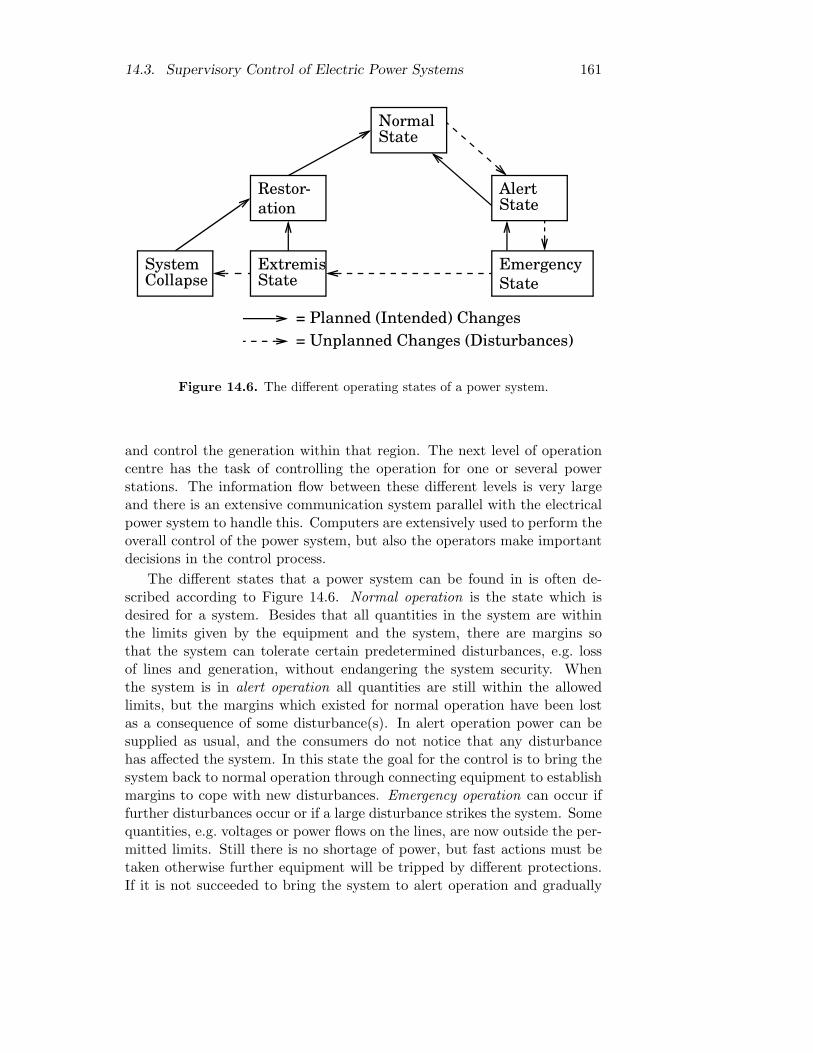
14.3. Supervisory Control of Electric Power Systems 161
Emergency
AlertState
NormalState
Restor-
ExtremisState
SystemCollapse
= Planned (Intended) Changes= Unplanned Changes (Disturbances)
State
ation
Figure 14.6. The different operating states of a power system.
and control the generation within that region. The next level of operationcentre has the task of controlling the operation for one or several powerstations. The information flow between these different levels is very largeand there is an extensive communication system parallel with the electricalpower system to handle this. Computers are extensively used to perform theoverall control of the power system, but also the operators make importantdecisions in the control process.
The different states that a power system can be found in is often de-scribed according to Figure 14.6. Normal operation is the state which isdesired for a system. Besides that all quantities in the system are withinthe limits given by the equipment and the system, there are margins sothat the system can tolerate certain predetermined disturbances, e.g. lossof lines and generation, without endangering the system security. Whenthe system is in alert operation all quantities are still within the allowedlimits, but the margins which existed for normal operation have been lostas a consequence of some disturbance(s). In alert operation power can besupplied as usual, and the consumers do not notice that any disturbancehas affected the system. In this state the goal for the control is to bring thesystem back to normal operation through connecting equipment to establishmargins to cope with new disturbances. Emergency operation can occur iffurther disturbances occur or if a large disturbance strikes the system. Somequantities, e.g. voltages or power flows on the lines, are now outside the per-mitted limits. Still there is no shortage of power, but fast actions must betaken otherwise further equipment will be tripped by different protections.If it is not succeeded to bring the system to alert operation and gradually
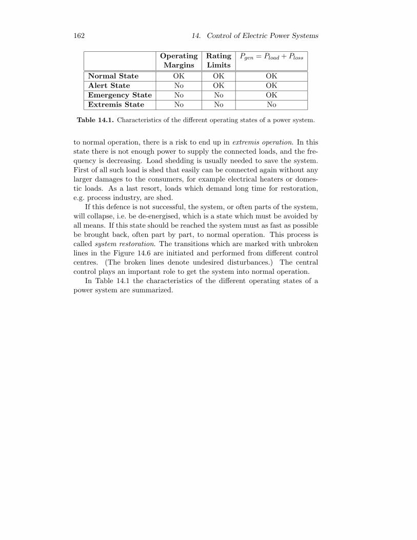
162 14. Control of Electric Power Systems
Operating Rating Pgen = Pload + Ploss
Margins Limits
Normal State OK OK OK
Alert State No OK OK
Emergency State No No OK
Extremis State No No No
Table 14.1. Characteristics of the different operating states of a power system.
to normal operation, there is a risk to end up in extremis operation. In thisstate there is not enough power to supply the connected loads, and the fre-quency is decreasing. Load shedding is usually needed to save the system.First of all such load is shed that easily can be connected again without anylarger damages to the consumers, for example electrical heaters or domes-tic loads. As a last resort, loads which demand long time for restoration,e.g. process industry, are shed.
If this defence is not successful, the system, or often parts of the system,will collapse, i.e. be de-energised, which is a state which must be avoided byall means. If this state should be reached the system must as fast as possiblebe brought back, often part by part, to normal operation. This process iscalled system restoration. The transitions which are marked with unbrokenlines in the Figure 14.6 are initiated and performed from different controlcentres. (The broken lines denote undesired disturbances.) The centralcontrol plays an important role to get the system into normal operation.
In Table 14.1 the characteristics of the different operating states of apower system are summarized.
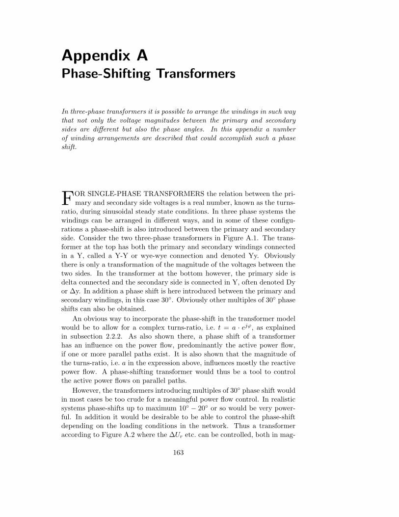
Appendix APhase-Shifting Transformers
In three-phase transformers it is possible to arrange the windings in such waythat not only the voltage magnitudes between the primary and secondarysides are different but also the phase angles. In this appendix a numberof winding arrangements are described that could accomplish such a phaseshift.
FOR SINGLE-PHASE TRANSFORMERS the relation between the pri-mary and secondary side voltages is a real number, known as the turns-
ratio, during sinusoidal steady state conditions. In three phase systems thewindings can be arranged in different ways, and in some of these configu-rations a phase-shift is also introduced between the primary and secondaryside. Consider the two three-phase transformers in Figure A.1. The trans-former at the top has both the primary and secondary windings connectedin a Y, called a Y-Y or wye-wye connection and denoted Yy. Obviouslythere is only a transformation of the magnitude of the voltages between thetwo sides. In the transformer at the bottom however, the primary side isdelta connected and the secondary side is connected in Y, often denoted Dyor ∆y. In addition a phase shift is here introduced between the primary andsecondary windings, in this case 30. Obviously other multiples of 30 phaseshifts can also be obtained.
An obvious way to incorporate the phase-shift in the transformer modelwould be to allow for a complex turns-ratio, i.e. t = a · ejϕ, as explainedin subsection 2.2.2. As also shown there, a phase shift of a transformerhas an influence on the power flow, predominantly the active power flow,if one or more parallel paths exist. It is also shown that the magnitude ofthe turns-ratio, i.e. a in the expression above, influences mostly the reactivepower flow. A phase-shifting transformer would thus be a tool to controlthe active power flows on parallel paths.
However, the transformers introducing multiples of 30 phase shift wouldin most cases be too crude for a meaningful power flow control. In realisticsystems phase-shifts up to maximum 10 − 20 or so would be very power-ful. In addition it would be desirable to be able to control the phase-shiftdepending on the loading conditions in the network. Thus a transformeraccording to Figure A.2 where the ∆Ur etc. can be controlled, both in mag-
163
164 A. Phase-Shifting Transformers
R S T
r
st
n
R
ST
r
st
R S Tr
s
t
n
R
ST
r
s
t
Figure A.1. Two different configurations of three-winding transformer.
nitude and in phase, would be of value. This is the so called regulatingtransformer.
The regulating function of these transformers is achieved through a tapchanger that can change the turns on one or more windings and therebychanging the turns-ratio. Depending on the design both the magnitudeand the phase of the turns-ratio could be changed. It is obvious that atap-changer in the transformer connection in Figure A.1 would only changethe magnitude of the turns-ratio. (It is assumed that the tap-changers onthe three phases are identical and operated identically.) Such arrangementscould thus only be used for voltage control. This is one of the main methodsto control the voltage in the distribution systems.
In order to introduce a controllable phase-shift to control the activepower flow more complicated winding configurations must be introduced.There are several ways of achieving this, and the solution chosen dependson a number of parameters, such as phase-shift range to be controlled, volt-age difference between the primary and secondary sides, power rating, etc.Phase-shifting transformers, or phase-shifters, are quite rare in comparisonto non phase-shifting transformers 1. However, phase-shifters play an im-
1With non phase-shifting transformers are here meant transformers where a possible
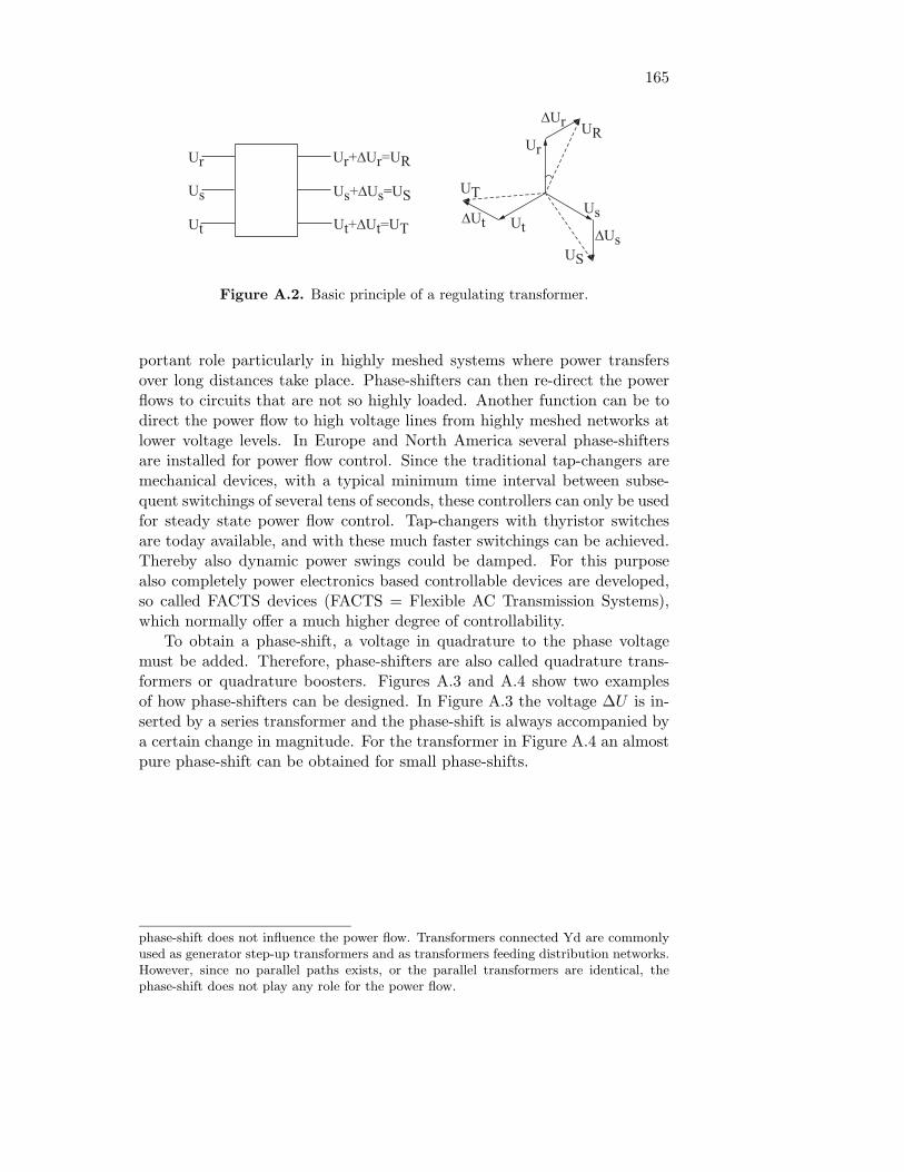
165
Ur
Us
Ut
Ur+ Ur=URD
Us+ Us=USD
Ut+ Ut=UTD
Ur
UsUt
UR
US
UT
DUr
DUs
DUt
Figure A.2. Basic principle of a regulating transformer.
portant role particularly in highly meshed systems where power transfersover long distances take place. Phase-shifters can then re-direct the powerflows to circuits that are not so highly loaded. Another function can be todirect the power flow to high voltage lines from highly meshed networks atlower voltage levels. In Europe and North America several phase-shiftersare installed for power flow control. Since the traditional tap-changers aremechanical devices, with a typical minimum time interval between subse-quent switchings of several tens of seconds, these controllers can only be usedfor steady state power flow control. Tap-changers with thyristor switchesare today available, and with these much faster switchings can be achieved.Thereby also dynamic power swings could be damped. For this purposealso completely power electronics based controllable devices are developed,so called FACTS devices (FACTS = Flexible AC Transmission Systems),which normally offer a much higher degree of controllability.
To obtain a phase-shift, a voltage in quadrature to the phase voltagemust be added. Therefore, phase-shifters are also called quadrature trans-formers or quadrature boosters. Figures A.3 and A.4 show two examplesof how phase-shifters can be designed. In Figure A.3 the voltage ∆U is in-serted by a series transformer and the phase-shift is always accompanied bya certain change in magnitude. For the transformer in Figure A.4 an almostpure phase-shift can be obtained for small phase-shifts.
phase-shift does not influence the power flow. Transformers connected Yd are commonlyused as generator step-up transformers and as transformers feeding distribution networks.However, since no parallel paths exists, or the parallel transformers are identical, thephase-shift does not play any role for the power flow.
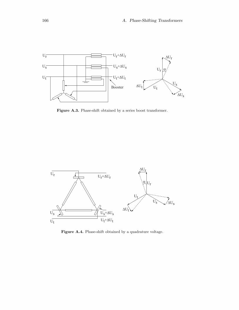
166 A. Phase-Shifting Transformers
Ur
Us
Ut
Ur+ UrD
Us+ UsD
Ut+ UtD
Ur
UsUt
DUr
DUs
DUt
a
Booster
Figure A.3. Phase-shift obtained by a series boost transformer.
Ur
Us
Ut
Ur+ UrD
Us+ UsD
Ut+ UtD
Ur
Us
Ut
DUr
DUs
DUt
a
Figure A.4. Phase-shift obtained by a quadrature voltage.
Appendix BProtections in Electric Power Systems
In this Appendix a brief summary of how protections are designed and howthey function is given. The very important distance protections and theiroperating principles are discussed. Some special protections and systemwide protections that are of relevance for power system stability is brieflyreviewed.
DIFFERENT TYPES of protections are installed to protect the equip-ment in an electric power system. Their task is to disconnect failed or
overloaded equipment or parts of the system to avoid unnecessary damageson equipment and personnel. The purpose is also to limit the impact offailures on the parts of the system that have not failed. Special types ofprotection are the “system protections”. Their task is to prevent collapse(black out) of the system or parts of the system.
An intensive development of protections based on modern informationtechnology is going on both regarding hardware and software. On the hard-ware side microprocessors have been used over a long time to implementdifferent functions in the protections, and with the recent developmentsmore and more complicated functions can be implemented in a reliable way.Powerful methods like signal processing, state estimation, and “artificialintelligence”, are being integrated into the protections. In general the func-tions which earlier were handled with separate relays are increasingly beingintegrated with other functional units for control and supervision. Further-more, more complicated criteria for activation of protections can be applied.The interested reader is referred to the literature for further information.The summary here is concentrated on general principles for protections.
B.1 Design of Protections
A protection for an electric power system comprises the following parts:
• Measurement device with current- and/or voltage transformers andother sensors measuring the relevant quantities.
• Relay which when certain conditions are fulfilled sends signals to acircuit breaker or another switching device. This relay was earlier a
167
168 B. Protections in Electric Power Systems
separate unit, but can in modern protections be a part of a larger unitfor protection, supervision and control.
• Circuit breakers which execute the given instruction(s) from the relay.
• Telecommunication system is mainly used at distance (line) protec-tions to get a faster and more reliable performance.
• Power supply systems which shall secure the power supply to the pro-tection system, even with faults in the system.
The requirements on a protection system are that they should be de-pendable, secure, selective, sensitive, and fast.
• Dependability means that the protection should react and do its actionwhen a fault occurs for which it is designed to react for. To achievedesired dependability double or even triple sets of certain parts of theprotection or of signal paths might be needed. Malfunctions can bedivided into ”not occurring” operations (which are actions that weresupposed to happen but did not) and ”unwanted” operations (whichare actions that happened although they should not have). Normallynot occurring operations are more serious malfunctions than unwantedones.
• Security means that the protection should not react when no faultoccurs or when a fault for which it is not intended to react occurs.
• Selectivity implies that not more than necessary pieces of equipmentand apparatuses are disconnected to isolate a fault.
• Sensitivity is needed to detect failures which cause small fault currents,e.g. high impedance faults. This implies that the risk for misoperationsincreases at “small” disturbances, e.g. at energisation of transformers,or at high load operation but normal operation.
• The protection should react fast to secure that damages on personsand equipment are prevented or limited.
The protections are often classified according to the object that theyprotect. An example is shown in Figure B.1. If a failure occurs within anindicated area in Figure B.1 this area should be isolated from the rest of thenetwork.
Many of the protections which protect separate pieces of equipment orparts of a system which occupy a limited physical area are so called currentdifferential protections. These protections measure the difference betweentwo currents, which in normal operation should be equal, and the protectionis activated if this deviation exceeds a predetermined value. Both differencesin amplitude and phase can trigger the relay. The principle for a currentdifferential protection is shown in Figure B.2.
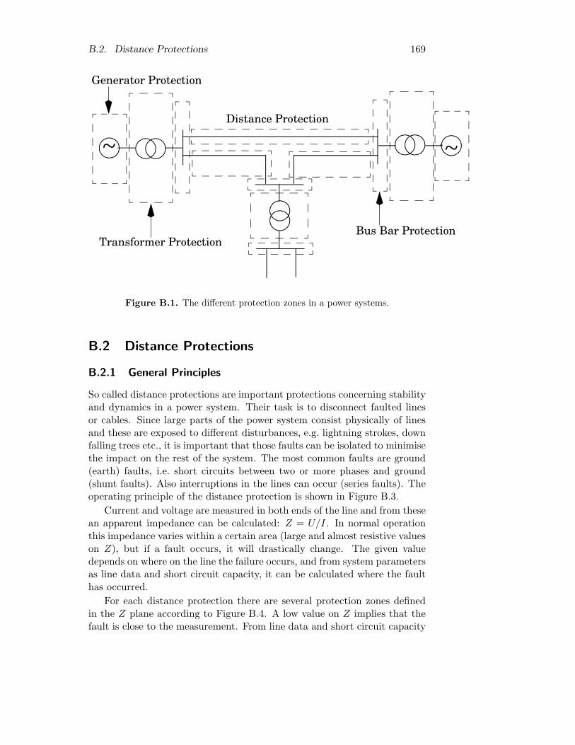
B.2. Distance Protections 169
~
~
Transformer Protection
Generator Protection
Bus Bar Protection
Distance Protection
Figure B.1. The different protection zones in a power systems.
B.2 Distance Protections
B.2.1 General Principles
So called distance protections are important protections concerning stabilityand dynamics in a power system. Their task is to disconnect faulted linesor cables. Since large parts of the power system consist physically of linesand these are exposed to different disturbances, e.g. lightning strokes, downfalling trees etc., it is important that those faults can be isolated to minimisethe impact on the rest of the system. The most common faults are ground(earth) faults, i.e. short circuits between two or more phases and ground(shunt faults). Also interruptions in the lines can occur (series faults). Theoperating principle of the distance protection is shown in Figure B.3.
Current and voltage are measured in both ends of the line and from thesean apparent impedance can be calculated: Z = U/I. In normal operationthis impedance varies within a certain area (large and almost resistive valueson Z), but if a fault occurs, it will drastically change. The given valuedepends on where on the line the failure occurs, and from system parametersas line data and short circuit capacity, it can be calculated where the faulthas occurred.
For each distance protection there are several protection zones definedin the Z plane according to Figure B.4. A low value on Z implies that thefault is close to the measurement. From line data and short circuit capacity
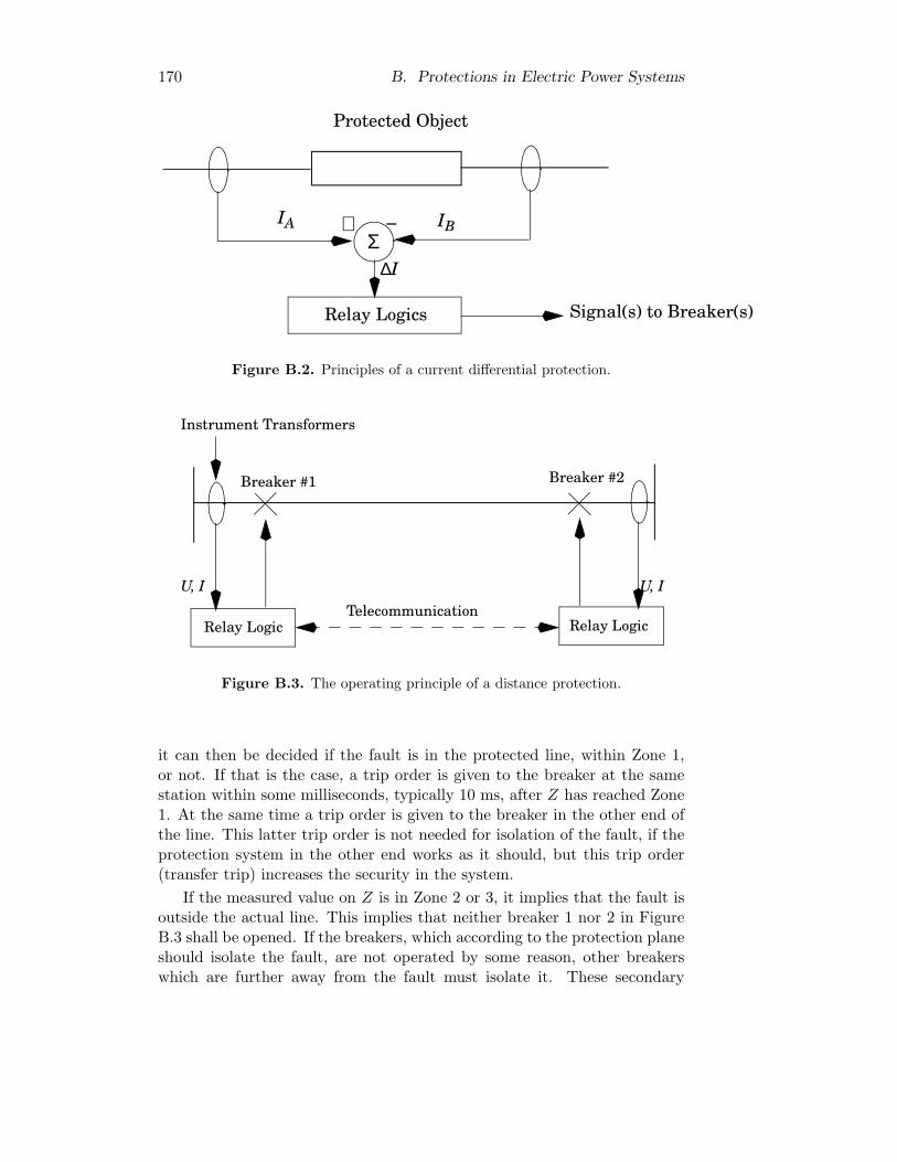
170 B. Protections in Electric Power Systems
IA IB
Protected Object
Σ+ −
∆I
Relay Logics Signal(s) to Breaker(s)
Figure B.2. Principles of a current differential protection.
Relay Logic Relay Logic
Breaker #1
Instrument Transformers
Telecommunication
U, I U, I
Breaker #2
Figure B.3. The operating principle of a distance protection.
it can then be decided if the fault is in the protected line, within Zone 1,or not. If that is the case, a trip order is given to the breaker at the samestation within some milliseconds, typically 10 ms, after Z has reached Zone1. At the same time a trip order is given to the breaker in the other end ofthe line. This latter trip order is not needed for isolation of the fault, if theprotection system in the other end works as it should, but this trip order(transfer trip) increases the security in the system.
If the measured value on Z is in Zone 2 or 3, it implies that the fault isoutside the actual line. This implies that neither breaker 1 nor 2 in FigureB.3 shall be opened. If the breakers, which according to the protection planeshould isolate the fault, are not operated by some reason, other breakerswhich are further away from the fault must isolate it. These secondary
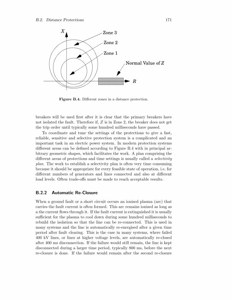
B.2. Distance Protections 171
Zone 3
Zone 2
Zone 1
Normal Value of Z
R
X
Figure B.4. Different zones in a distance protection.
breakers will be used first after it is clear that the primary breakers havenot isolated the fault. Therefore if, Z is in Zone 2, the breaker does not getthe trip order until typically some hundred milliseconds have passed.
To coordinate and tune the settings of the protections to give a fast,reliable, sensitive and selective protection system is a complicated and animportant task in an electric power system. In modern protection systemsdifferent areas can be defined according to Figure B.4 with in principal ar-bitrary geometric shapes, which facilitates the work. A plan comprising thedifferent areas of protections and time settings is usually called a selectivityplan. The work to establish a selectivity plan is often very time consumingbecause it should be appropriate for every feasible state of operation, i.e. fordifferent numbers of generators and lines connected and also at differentload levels. Often trade-offs must be made to reach acceptable results.
B.2.2 Automatic Re-Closure
When a ground fault or a short circuit occurs an ionised plasma (arc) thatcarries the fault current is often formed. This arc remains ionised as long asa the current flows through it. If the fault current is extinguished it is usuallysufficient for the plasma to cool down during some hundred milliseconds torebuild the isolation so that the line can be re-connected. This is used inmany systems and the line is automatically re-energised after a given timeperiod after fault clearing. This is the case in many systems, where failed400 kV lines, or lines at higher voltage levels, are automatically re-closedafter 400 ms disconnection. If the failure would still remain, the line is keptdisconnected during a larger time period, typically 800 ms, before the nextre-closure is done. If the failure would remain after the second re-closure
172 B. Protections in Electric Power Systems
attempt, more attempts to re-close will not be made. In this latter case theisolation of the line has probably been permanently damaged and it mustbe repaired before the line can be put in operation again. (This scenariois typical. Due to specific conditions in different countries, deviations canoccur.)
Automatic re-closure must be made with certain carefulness when it ismade close to large thermal power plants, e.g. nuclear power plants. Theconnection can in this case cause large stresses on the generator shaft if itoccurs at certain phase positions. The re-closure can in this case be done inthe remote end of the line seen from the thermal power plant, and then asynchronised re-closure at the other end is made. (With synchronised closureis meant that the voltage over the breaker is zero when it is closed.) In thatway the transients in the system are drastically reduced, but of course there-closure takes longer time.
In some systems all fault clearings on the high voltage grid are made onall three phases. In other systems one phase clearing is used. This meansthat only the faulty phase(s) is (are) disconnected at fault clearing and re-closure.
B.3 Out of Step Protections
A synchronous machine which has fallen out of step, i.e. its angular velocitydoes not coincide with the angular velocity of the net, has lost the synchro-nism with the system, and the machine must be disconnected. In order tosupply electrical power to the system it must be phased in to the systemlater on. During the time period when the synchronous machine falls outof step large current pulses will pass through the generator, and if thesebecome too many they can damage the generator and limit its life time.Furthermore, vibrations that can jeopardise the generator can arise. Toprotect a synchronous machine which has fallen out of step the synchronousmachine is equipped with a out of step relay.
Also in this case an impedance is defined from voltage and current. If theoperation state of the generator is in the critical impedance zone a clock isstarted. If the generator then comes into the critical zone repeatedly times,this is a criterion that the generator is falling out of step, and the protectiongives a trip order to the generator breakers.
Generators are also equipped with other protections against overload(stator current protection), over-excitation, etc.
B.4 System Protections
System protections are special types of protection, the primary task of whichis not to isolate failed equipment, but to prevent that the total system or
B.4. System Protections 173
large parts of it collapse. System protections often use information fromseveral different points in the system or quantities which can give a reliablediagnosis of the state of the system. These systems often work in a timescale which is considerably longer than the more device oriented protectionswhich were considered earlier, typically several seconds or minutes. Anexample of a system protection is load shedding. This is used to avoid thatthe frequency in the system falls below acceptable values if the generationcapacity has dropped in the system. The load shedding then disconnectspredetermined loads depending on how much and how fast the frequency isfalling. Voltage collapse protection is another system protection, the task ofwhich is to prevent voltage collapse in the system. Load shedding uses onlythe frequency as input signal, while the voltage collapse protection oftenuses several different quantities as input signals.