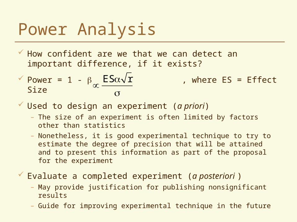
Power Analysis How confident are we that we can detect an important

difference, if it exists?

Power = 1 - , where ES = Effect Size

Used to design an experiment (a priori)– The size of an experiment is often limited by factors other than

statistics

– Nonetheless, it is good experimental technique to try to estimate the degree of precision that will be attained and to present this information as part of the proposal for the experiment

Evaluate a completed experiment (a posteriori )– May provide justification for publishing nonsignificant results

– Guide for improving experimental technique in the future

ES r

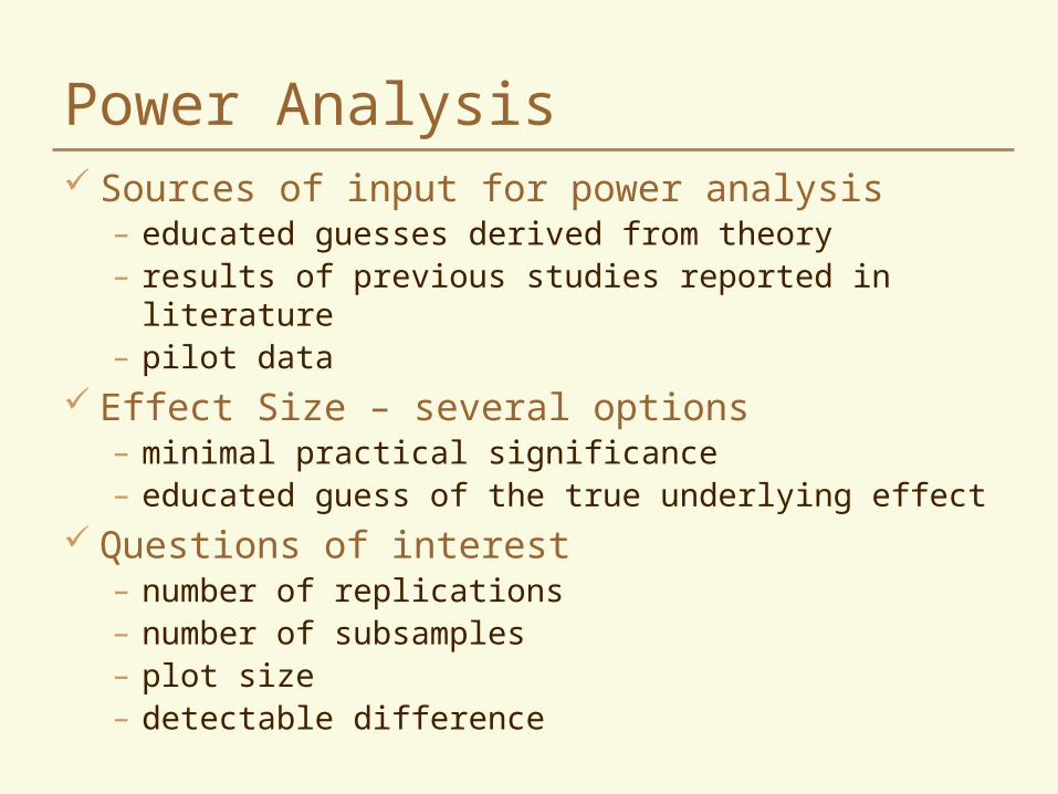
Power Analysis Sources of input for power analysis

– educated guesses derived from theory– results of previous studies reported in literature– pilot data

Effect Size – several options– minimal practical significance– educated guess of the true underlying effect

Questions of interest– number of replications– number of subsamples– plot size– detectable difference

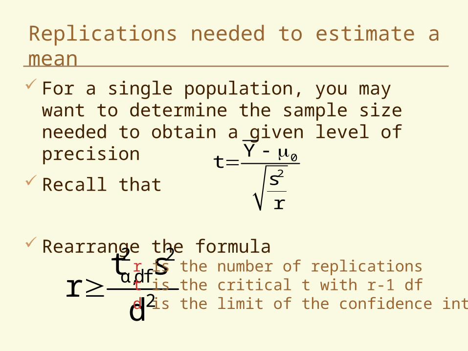
Replications needed to estimate a mean

For a single population, you may want to determine the sample size needed to obtain a given level of precision

Recall that

Rearrange the formula

0

2

Yt

sr

2 2α,df

2

t sr

d

r is the number of replicationst is the critical t with r-1 dfd is the limit of the confidence interval

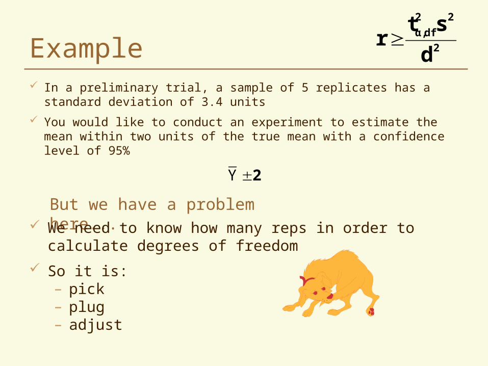
Example In a preliminary trial, a sample of 5 replicates has a standard

deviation of 3.4 units

You would like to conduct an experiment to estimate the mean within two units of the true mean with a confidence level of 95%

2

22

dfα,

d

str

But we have a problem here...

2Y

We need to know how many reps in order to calculate degrees of freedom

So it is:– pick– plug– adjust

Calculations

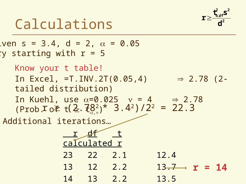
Know your t table!In Excel, =T.INV.2T(0.05,4) 2.78 (2-tailed distribution)In Kuehl, use =0.025 = 4 2.78 (Prob. of t t,)

Given s = 3.4, d = 2, = 0.05 Try starting with r = 5

r (2.782 * 3.42)/22 = 22.3

r df t calculated r

23 22 2.1 12.4

13 12 2.2 13.7

14 13 2.2 13.5 r = 14

Additional iterations…

2

22

dfα,

d

str

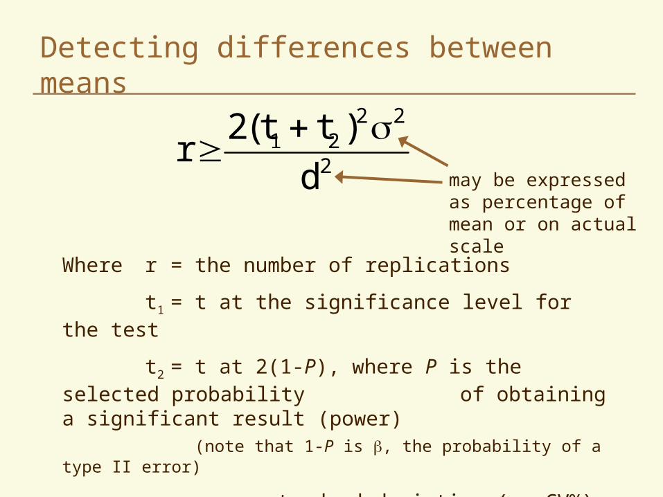
Detecting differences between means

may be expressed as percentage of mean or on actual scale

Where r = the number of replications

t1 = t at the significance level for the test

t2 = t at 2(1-P), where P is the selected probability of obtaining a significant result (power)(note that 1-P is , the probability of a type II error)

= standard deviation (or CV%)

d = the difference that it is desired to detect

2 21 2

2

2(t t )r

d

What is meaningful? If it can be established that the new is

superior to the old by at least some stated amount, say 20%, then we will have discovered a useful result

If the experiment shows no significant difference, we will be discouraged from further investigation

The experiment should be large enough to ensure a meaningful difference.

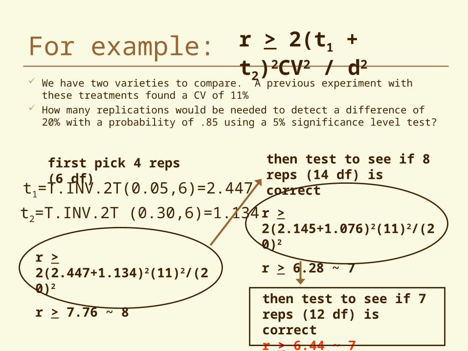
For example: We have two varieties to compare. A previous experiment with these

treatments found a CV of 11% How many replications would be needed to detect a difference of 20%

with a probability of .85 using a 5% significance level test?

r > 2(t1 + t2)2CV2 / d2

r > 2(2.447+1.134)2(11)2/(20)2

r > 7.76 ~ 8

first pick 4 reps (6 df)

r > 2(2.145+1.076)2(11)2/(20)2

r > 6.28 ~ 7

then test to see if 8 reps (14 df) is correct

t1=T.INV.2T(0.05,6)=2.447

t2=T.INV.2T (0.30,6)=1.134

then test to see if 7 reps (12 df) is correctr > 6.44 ~ 7

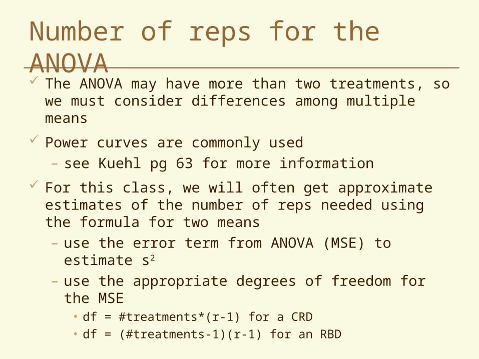
Number of reps for the ANOVA The ANOVA may have more than two treatments, so we

must consider differences among multiple means

Power curves are commonly used– see Kuehl pg 63 for more information

For this class, we will often get approximate estimates of the number of reps needed using the formula for two means– use the error term from ANOVA (MSE) to estimate s2

– use the appropriate degrees of freedom for the MSE• df = #treatments*(r-1) for a CRD• df = (#treatments-1)(r-1) for an RBD

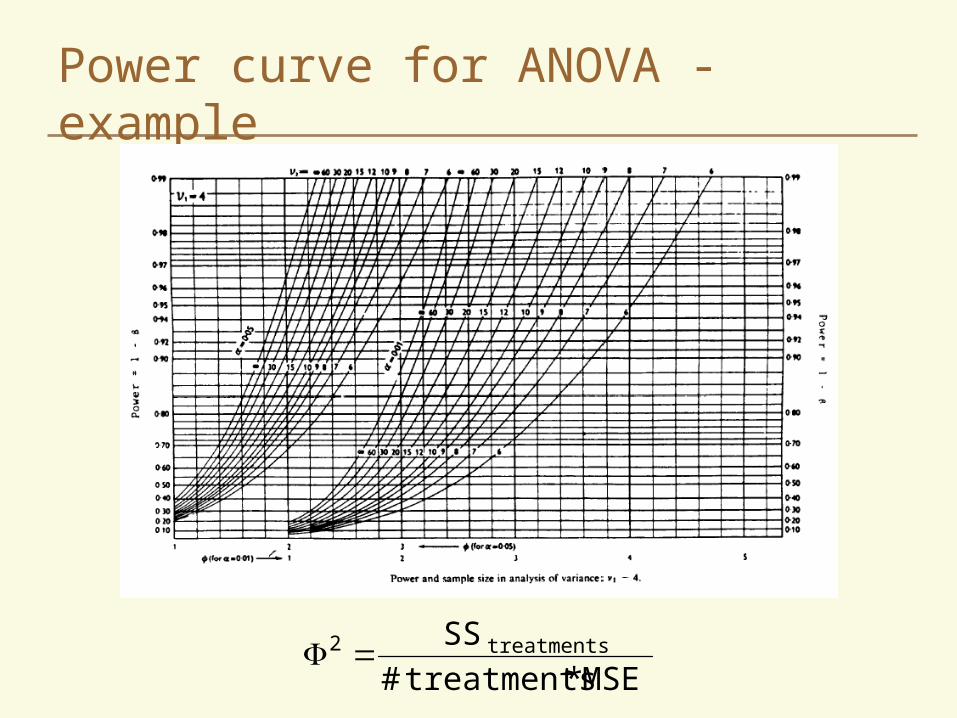
Power curve for ANOVA - example

MSE*treatments#

SStreatments2

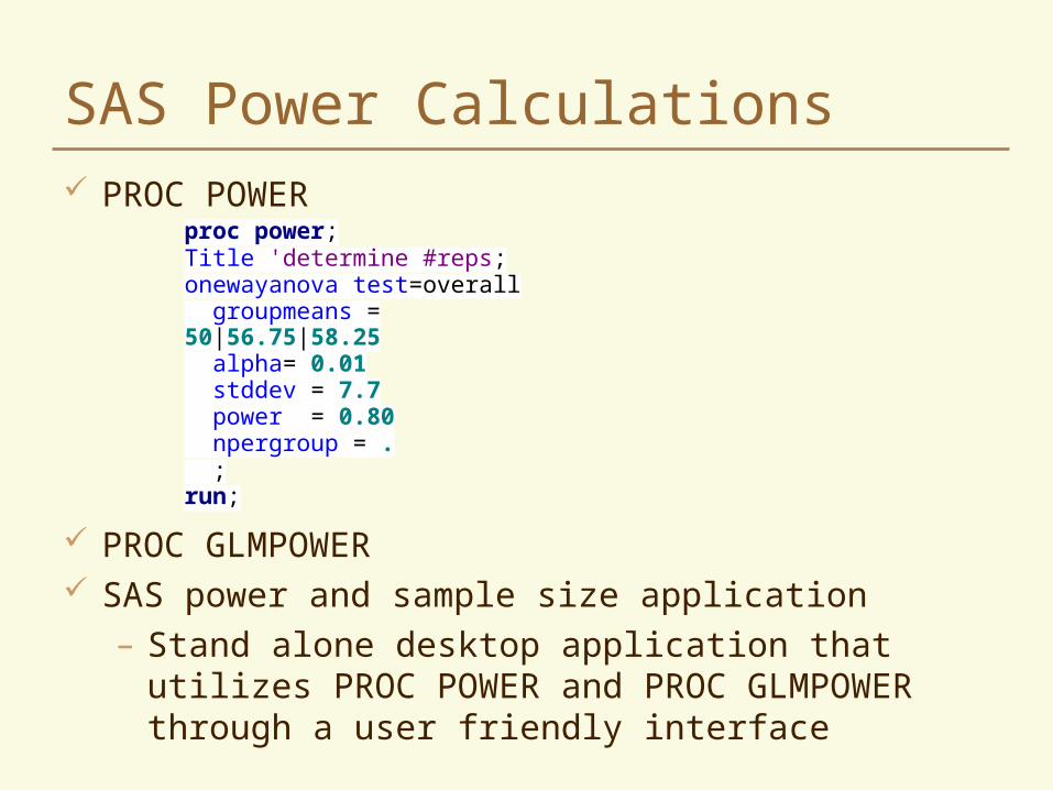
SAS Power Calculations PROC POWER

PROC GLMPOWER SAS power and sample size application

– Stand alone desktop application that utilizes PROC POWER and PROC GLMPOWER through a user friendly interface

proc power; Title 'determine #reps; onewayanova test=overall groupmeans = 50|56.75|58.25 alpha= 0.01 stddev = 7.7 power = 0.80 npergroup = . ; run;

Determining Plot Size

Factors that affect plot size Type of crop

Type of experiment

Phase of the research program

Variability of the experimental site

Presence and nature of border effects

Type of machinery to be used

Number and type of treatments

Land area available

Cost

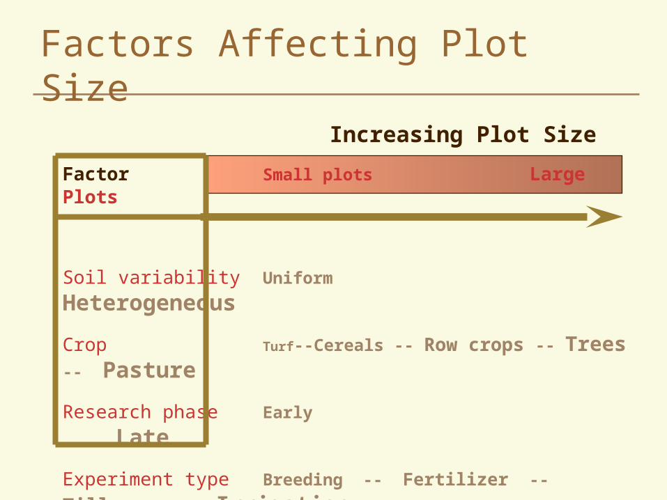
Increasing Plot Size

Factor Small plots Large Plots

Soil variability Uniform Heterogeneous

Crop Turf--Cereals -- Row crops -- Trees -- Pasture

Research phase Early Late

Experiment type Breeding -- Fertilizer -- Tillage -- Irrigation

Machinery None Research Farm Scale

Factors Affecting Plot Size

Effect on Variability

Variability per plot decreases as plot size increases

But large plots may yield higher experimental error because of larger more variable area for the experiment

Very small plots are highly variable because:– Losses at harvest and measurement errors

have a greater effect– Reduced plant numbers– Competition and border effects are greater

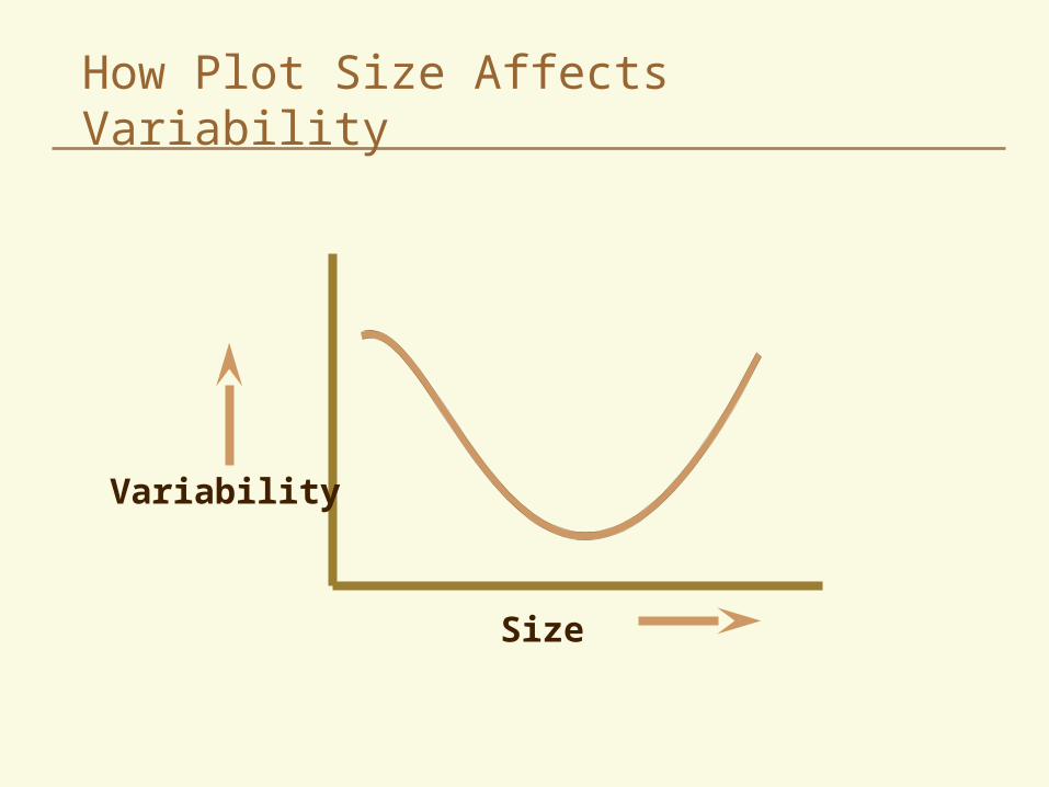
How Plot Size Affects Variability

Variability

Size

Plot Size ‘Rule of Thumb’

There are some lower limits:– Should be large enough to permit

removal of borders with enough left over to harvest and measure adequately

– Should be large enough to handle the machinery needed

Once the plots are large enough to be handled conveniently, precision is increased faster by increasing the number of replications

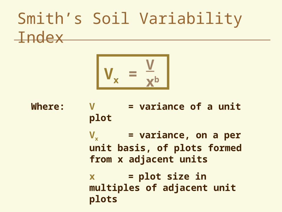
Smith’s Soil Variability Index

Vx =Vxb

Where: V = variance of a unit plot

Vx = variance, on a per unit basis, of plots formed from x adjacent units

x = plot size in multiples of adjacent unit plots

b = index of soil variability

Smith’s Soil Variability Index

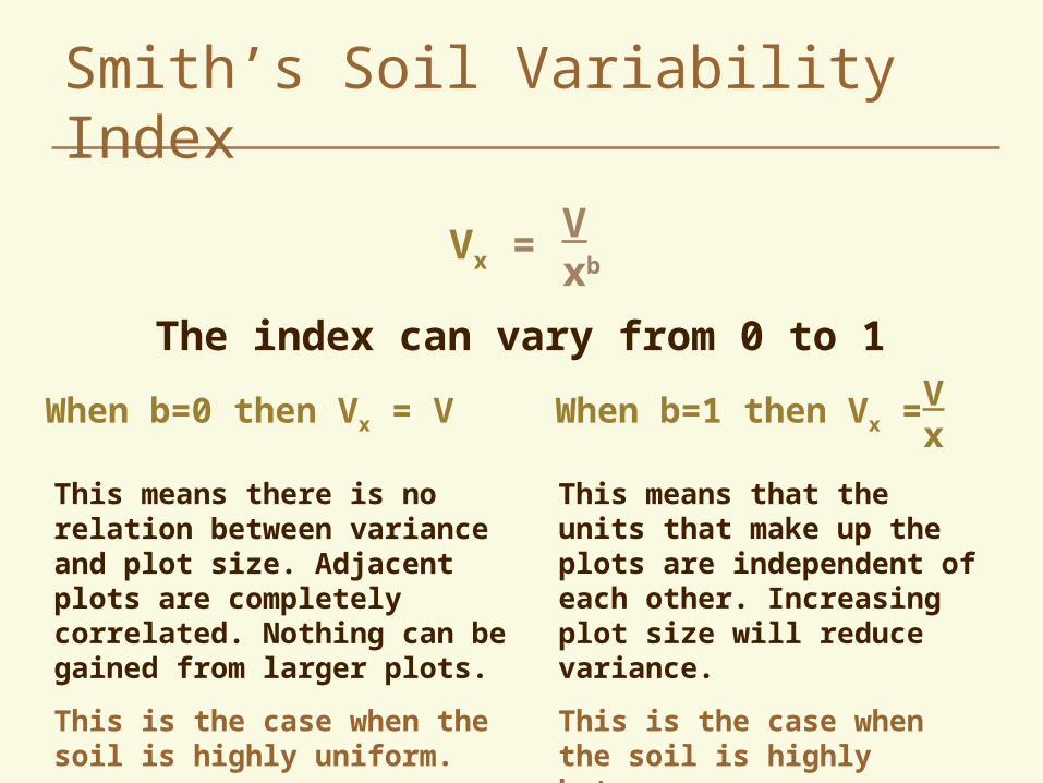
The index can vary from 0 to 1

When b=0 then Vx = V

This means there is no relation between variance and plot size. Adjacent plots are completely correlated. Nothing can be gained from larger plots.

This is the case when the soil is highly uniform.

When b=1 then Vx = Vx

This means that the units that make up the plots are independent of each other. Increasing plot size will reduce variance.

This is the case when the soil is highly heterogeneous.

Vx =Vxb

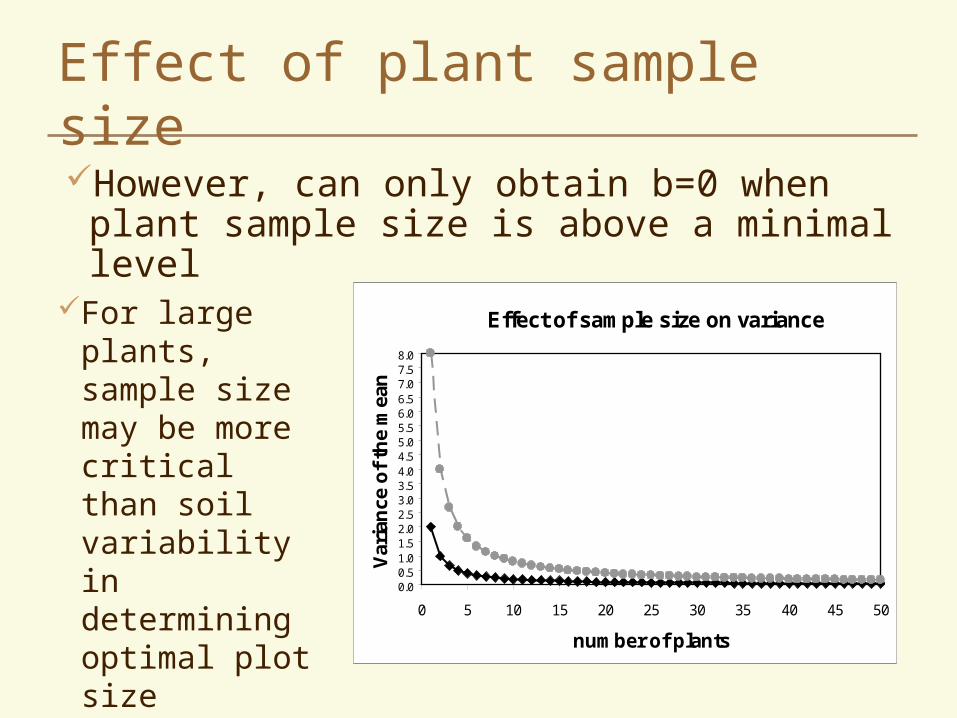
Effect of plant sample size

However, can only obtain b=0 when plant sample size is above a minimal level

Effect of sample size on variance

0.00.51.01.52.02.53.03.54.04.55.05.56.06.57.07.58.0

0 5 10 15 20 25 30 35 40 45 50

number of plants

Var

ian

ce o

f th

e m

ean

For large plants, sample size may be more critical than soil variability in determining optimal plot size

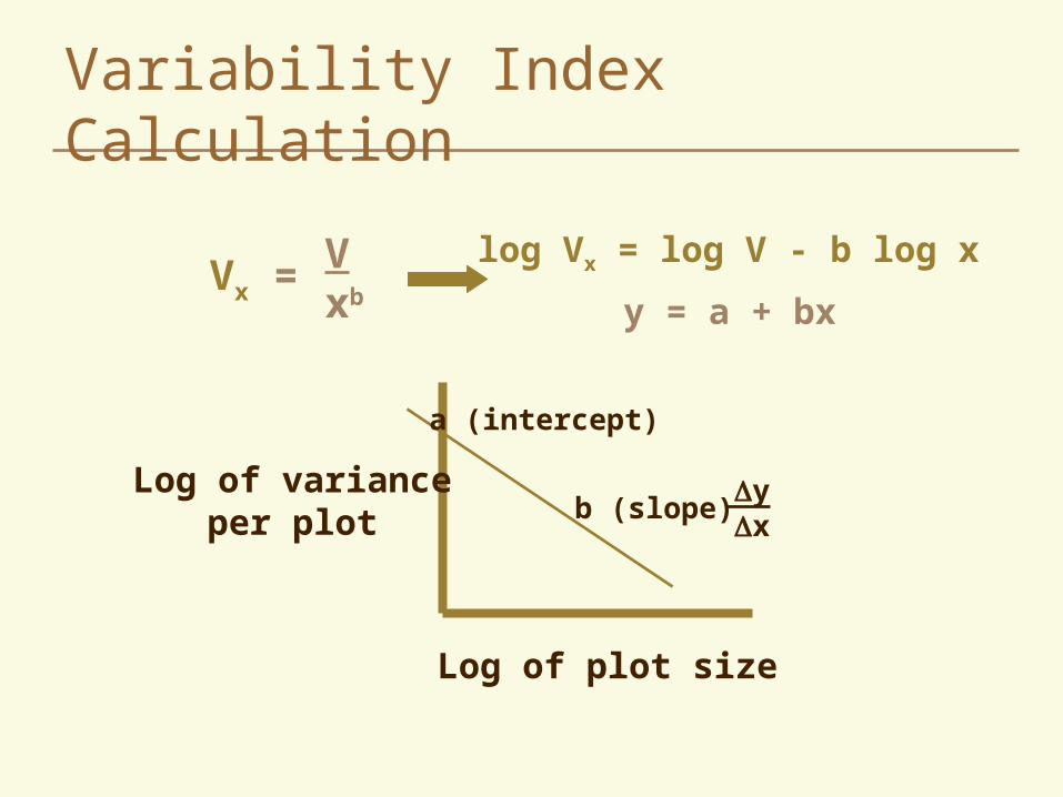
Variability Index Calculation

log Vx = log V - b log x

y = a + bx

Log of plot size

Log of varianceper plot

a (intercept)

b (slope)yx

Vx =Vxb

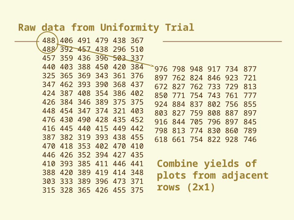
488 406 491 479 438 367 488 392 457 438 296 510 457 359 436 396 503 337 440 403 388 450 420 384 325 365 369 343 361 376 347 462 393 390 368 437 424 387 408 354 386 402 426 384 346 389 375 375 448 454 347 374 321 403 476 430 490 428 435 452 416 445 440 415 449 442 387 382 319 393 438 455 470 418 353 402 470 410 446 426 352 394 427 435 410 393 385 411 446 441 388 420 389 419 414 348 303 333 389 396 473 371 315 328 365 426 455 375

976 798 948 917 734 877 897 762 824 846 923 721 672 827 762 733 729 813 850 771 754 743 761 777 924 884 837 802 756 855 803 827 759 808 887 897 916 844 705 796 897 845 798 813 774 830 860 789 618 661 754 822 928 746

Raw data from Uniformity Trial

Combine yields of plots from adjacent rows (2x1)

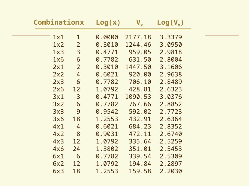
1x1 1 0.0000 2177.18 3.3379 1x2 2 0.3010 1244.46 3.0950 1x3 3 0.4771 959.05 2.9818 1x6 6 0.7782 631.50 2.8004 2x1 2 0.3010 1447.50 3.1606 2x2 4 0.6021 920.00 2.9638 2x3 6 0.7782 706.10 2.8489 2x6 12 1.0792 428.81 2.6323 3x1 3 0.4771 1090.53 3.0376 3x2 6 0.7782 767.66 2.8852 3x3 9 0.9542 592.02 2.7723 3x6 18 1.2553 432.91 2.6364 4x1 4 0.6021 684.23 2.8352 4x2 8 0.9031 472.11 2.6740 4x3 12 1.0792 335.64 2.5259 4x6 24 1.3802 351.01 2.5453 6x1 6 0.7782 339.54 2.5309 6x2 12 1.0792 194.84 2.2897 6x3 18 1.2553 159.58 2.2030

Combination x Log(x) Vx Log(Vx)

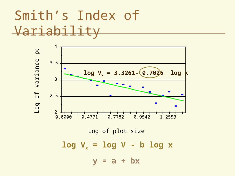
Smith’s Index of Variability

2

2.5

3

3.5

4

Lo

g o

f va

ria

nce

pe

r p

lot

0.0000 0.4771 0.7782 0.9542 1.2553

Log of plot size

log Vx = 3.3261- 0.7026 log x

log Vx = log V - b log x

y = a + bx

Is there an easier way?

Examination of a large number of data sets indicated that a value of b=0.5 may serve as a reasonable approximation.

“Finagles” constant b=0.5

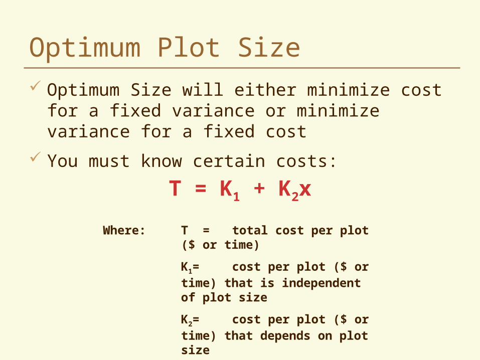
Optimum Plot Size Optimum Size will either minimize cost for a fixed

variance or minimize variance for a fixed cost

You must know certain costs:

T = K1 + K2x

Where: T = total cost per plot ($ or time)

K1= cost per plot ($ or time) that is independent of plot size

K2= cost per plot ($ or time) that depends on plot size

x = number of unit plots

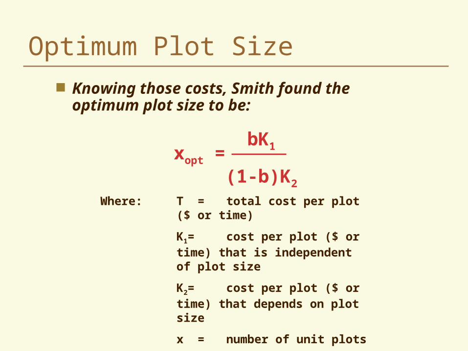
Optimum Plot Size Knowing those costs, Smith found the

optimum plot size to be:

xopt =bK1

(1-b)K2

Where: T = total cost per plot ($ or time)

K1= cost per plot ($ or time) that is independent of plot size

K2= cost per plot ($ or time) that depends on plot size

x = number of unit plots

b = Smith’s index of soil variability

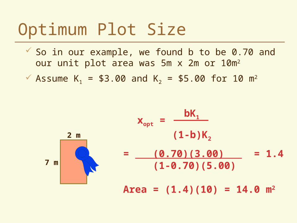
Optimum Plot Size So in our example, we found b to be 0.70 and our unit

plot area was 5m x 2m or 10m2

Assume K1 = $3.00 and K2 = $5.00 for 10 m2

= (0.70)(3.00) = 1.4 (1-0.70)(5.00)

Area = (1.4)(10) = 14.0 m2

2 m

7 m

xopt =bK1

(1-b)K2

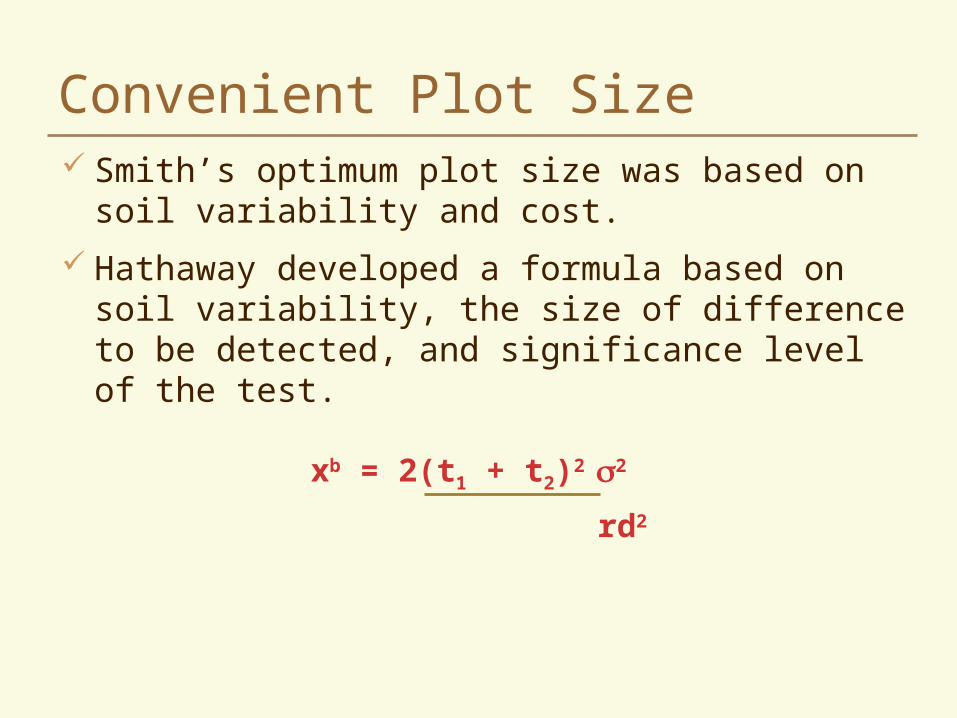
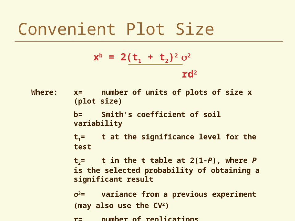
Convenient Plot Size Smith’s optimum plot size was based on soil

variability and cost.

Hathaway developed a formula based on soil variability, the size of difference to be detected, and significance level of the test.

xb = 2(t1 + t2)2 2

rd2

Convenient Plot Size

Where: x= number of units of plots of size x (plot size)

b= Smith’s coefficient of soil variability

t1= t at the significance level for the test

t2= t in the t table at 2(1-P), where P is the selected probability of obtaining a significant result

2= variance from a previous experiment (may

also use the CV2)

r= number of replications

d= difference to be detected (may be an absolute amount or expressed as percentage of the mean)

xb = 2(t1 + t2)2 2

rd2

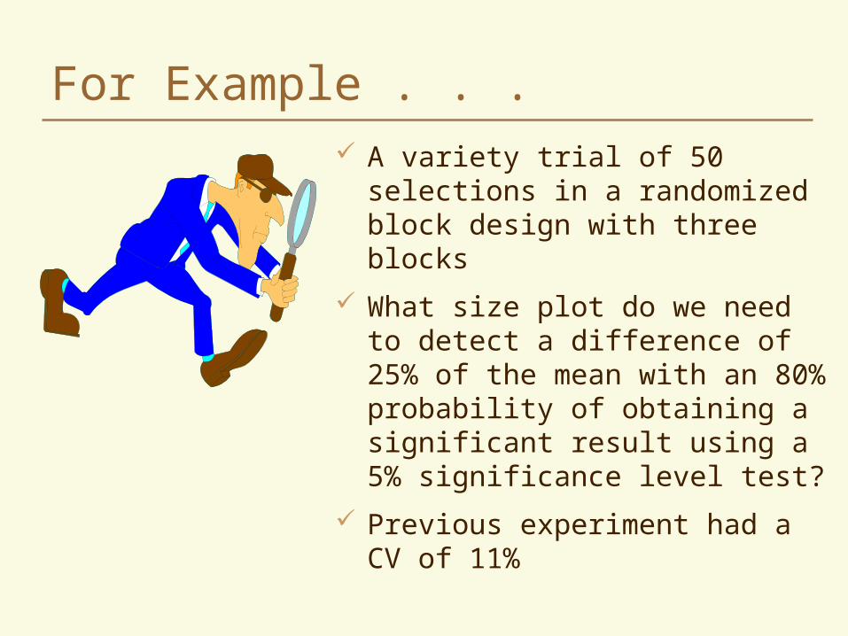
For Example . . . A variety trial of 50 selections in a

randomized block design with three blocks

What size plot do we need to detect a difference of 25% of the mean with an 80% probability of obtaining a significant result using a 5% significance level test?

Previous experiment had a CV of 11%

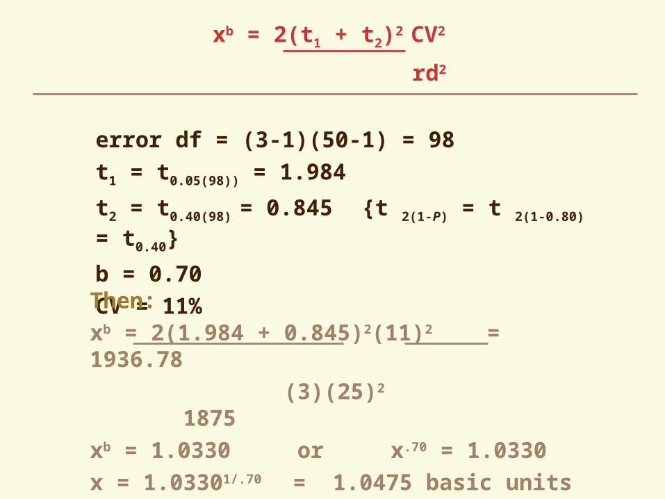
xb = 2(t1 + t2)2 CV2

rd2

error df = (3-1)(50-1) = 98

t1 = t0.05(98)) = 1.984

t2 = t0.40(98) = 0.845 {t 2(1-P) = t 2(1-0.80) = t0.40}

b = 0.70

CV = 11%Then:

xb = 2(1.984 + 0.845)2(11)2 = 1936.78 (3)(25)2 1875

xb = 1.0330 or x.70 = 1.0330

x = 1.03301/.70 = 1.0475 basic units

Convenient Plot Size Since the basic plot has an area of 10 m2, the

required plot size would be:

(10.00)(1.0475) = 10.48 m2

2 m

5.24 m

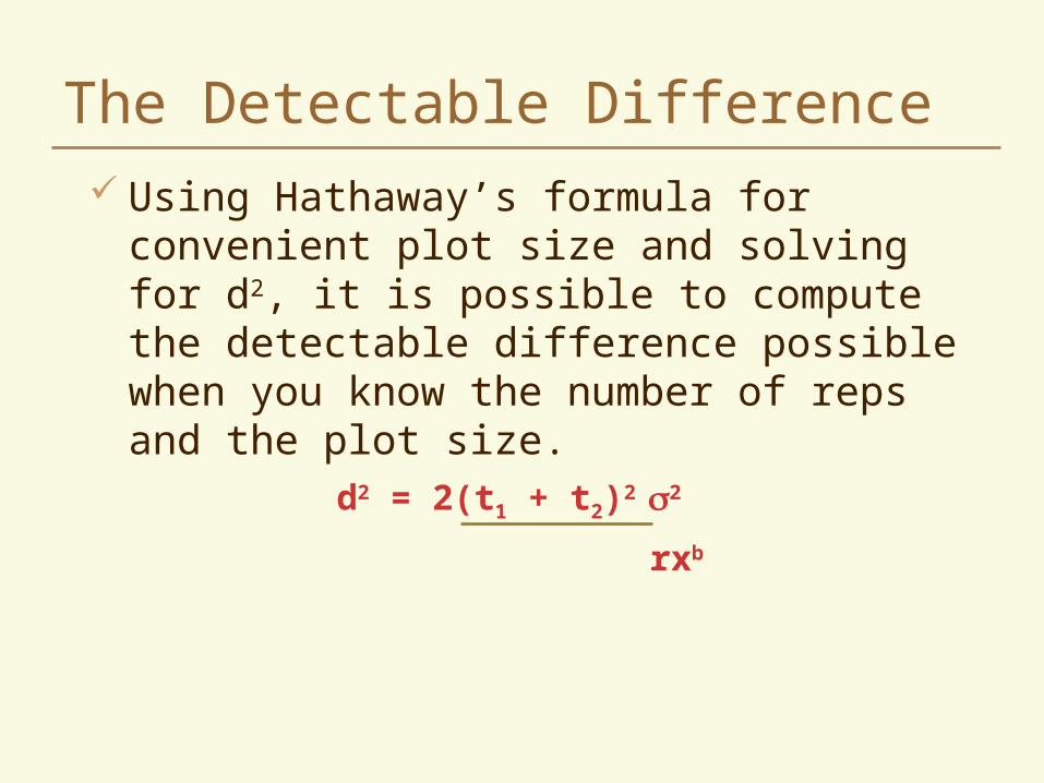
The Detectable Difference Using Hathaway’s formula for convenient plot

size and solving for d2, it is possible to compute the detectable difference possible when you know the number of reps and the plot size.

d2 = 2(t1 + t2)2 2

rxb

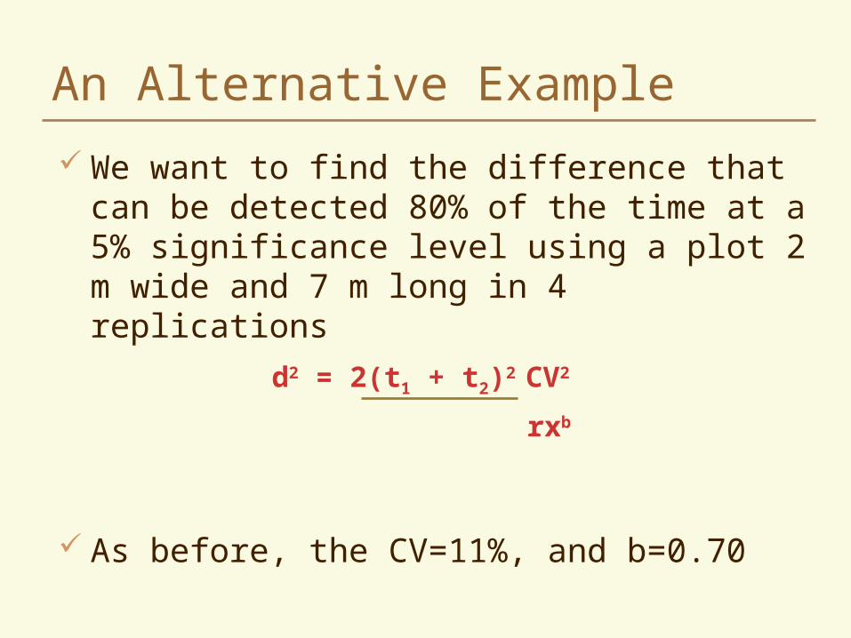
An Alternative Example

We want to find the difference that can be detected 80% of the time at a 5% significance level using a plot 2 m wide and 7 m long in 4 replications

As before, the CV=11%, and b=0.70

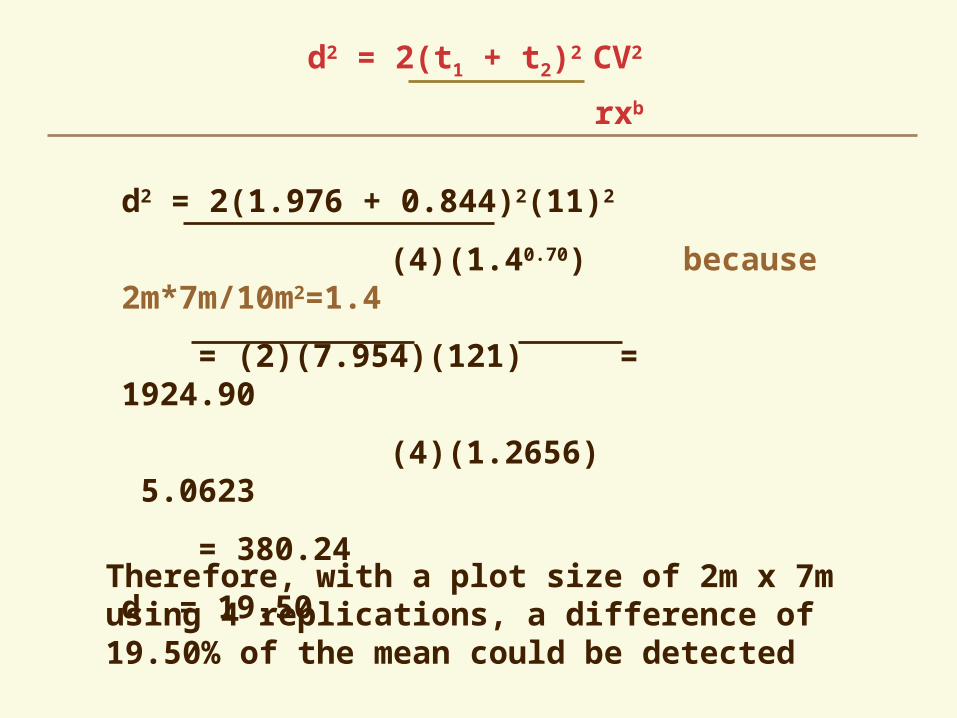
d2 = 2(t1 + t2)2 CV2

rxb

d2 = 2(t1 + t2)2 CV2

rxb

d2 = 2(1.976 + 0.844)2(11)2

(4)(1.40.70) because 2m*7m/10m2=1.4

= (2)(7.954)(121) = 1924.90

(4)(1.2656) 5.0623

= 380.24

d = 19.50

Therefore, with a plot size of 2m x 7m using 4 replications, a difference of 19.50% of the mean could be detected

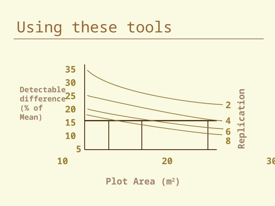
Using these tools

35

30

25

20

15

10

5 10 20 30

2

468

Detectabledifference(% ofMean)

Plot Area (m2)

Rep

lica

tio

n