IOP PUBLISHING JOURNAL OF GEOPHYSICS AND ENGINEERING

J. Geophys. Eng. 6 (2009) 325–344 doi:10.1088/1742-2132/6/4/001

Porosity and permeability estimation byintegration of production and time-lapsenear and far offset seismic dataMohsen Dadashpour1, David Echeverrıa-Ciaurri2, Jon Kleppe1 andMartin Landrø2

1 Department of Petroleum Engineering and Applied Geophysics, NTNU, 7491, Trondheim,Norway2 Department of Energy Resources Engineering, 367 Panama Street, Green Earth Sciences,Stanford University, Stanford, CA 94305-2220, USA

E-mail: dadashpour.mohsen@ntnu.no, jon.kleppe@ntnu.no, martin.landro@ntnu.no anddavid.Echeverria@stanford.edu

Received 19 February 2009Accepted for publication 14 August 2009Published 8 September 2009Online at stacks.iop.org/JGE/6/325

AbstractThis study presents a method based on the Gauss–Newton optimization technique forcontinuous reservoir model updating with respect to production history and time-lapse seismicdata in the form of zero offset amplitudes and amplitude versus offset (AVO) gradients. Themain objective of the study is to test the feasibility of using these integrated data as input toreservoir parameter estimation problems. Using only production data or zero offset time-lapseseismic amplitudes as observation data in the parameter estimation process cannot properlylimit the solution space. The emphasis of this work is to use the integrated data combined withempirical knowledge about rock types from laboratory measurements, to further constrain theinversion process. The algorithm written for this study consists of three parts: the reservoirsimulator, the rock physics petro-elastic model and the optimization algorithm. TheGauss–Newton inversion is tested at a 2D semi-synthetic model inspired by real field datafrom offshore Norway. The algorithm reduces the misfit between the observed and simulateddata which make it possible to estimate porosity and permeability distributions. TheGauss–Newton optimization technique is an efficient parameter estimation technique.However, the numerical estimation of the gradient is time consuming, and it can be prohibitivefor practical applications. This method is suitable for distributed computing whichconsiderably reduces the total optimization time. The amount of reduction depends mainly onthe number of available processors.

Keywords: time-lapse seismic, parameter estimation, simulation based optimization, AVOgradient, zero offset amplitudes

Nomenclature

c the average number of contacts per grainCp data noise covariance matrixCs data noise covariance matrixdp vector of observed production historical datadS vector of observed time-lapse seismic differencesF objective function

G gradient matrixH Hessian matrixJ Jacobin matrixK permeability, mDkf the bulk modulus of the saturating fluidkfr the bulk modulus of the solid frameworkkHM bulk modulus of the Hertz–Mindlin formulakma matrix bulk modulus

1742-2132/09/040325+20$30.00 © 2009 Nanjing Institute of Geophysical Prospecting Printed in the UK 325

M Dadashpour et al

ko oil bulk modulussw water bulk moduluskg gas bulk modulusMP(θ ) the vectors of simulated reservoir production

historiesMP(θ∗) the vectors of simulated reservoir production

historiesMS(θ ) the vectors of simulated time-lapse seismic

differencesMS(θ∗) the vectors of simulated time-lapse seismic

differencesn the coordination numberP hydrostatic pressurePeff is the effective pressurePext the lithostatic pressureSo oil saturationSw oil saturationSg oil saturationVPSH shale P-wave velocityVSSH shale S-wave velocityWBHPI well bottom hole pressure for the injectorWBHPP well bottom hole pressure for the producerWOPR well oil production rateWWPRI well water production rateρma matrix densityρo oil densityρw water densityρs gas densityρSH shale densityϕ effective porosityϕc critical porosityθ vector of unknown reservoir model parametersμ shear modulus of the solid phaseμHM shear modulus of the Hertz–Mindlin formulaν Poisson’s ratioˆ scaled (Hessian, gradient, . . . )

1. Introduction

So far, parameter estimation, using new geophysicalknowledge such as time-lapse seismic data, is a new andprobably underdeveloped method. The main challenge is toobtain a method for the estimation of key reservoir parameterswith the lowest possible estimation error. History matchingusing time-lapse seismic is relatively new (Landa and Horne1997, Minkoff et al 1998, Huang et al 2000, Kertz et al 2002,Gosselin et al 2003, Mezghani et al 2004, Yannong and Oliver2005, Skorstad et al 2006, Stephen et al 2006, Walker and Lane2007). Our approach contains two new elements compared tothe works cited above:

• the use of amplitude versus offset (AVO) time-lapse data,• the use of empirical rock physics relations.

The inversion process is non-unique, which is the primaryreason for using time-lapse information, in addition to otherdata, to limit the solution space. Additionally, time-lapseseismic data provide information between wells. It istherefore, an important spatial, complementary data source.Time-lapse seismic technology was first introduced in the early

1980s, and many works have been published since that timeconcerning this area (Greaves and Fulp 1987, Lumley et al1994, Landrø et al 1999, Koster et al 2000, Landrø 2001,Furre et al 2003, Vasco et al 2004).

Time-lapse seismic data are time-dependent dynamicmeasurements whose aim is to determine reservoir changesthat have occurred in the intervening time (Eastwood et al1994, Lazaratos and Marion 1997, Landrø et al 1999, Burkhartet al 2000, Behrens et al 2002). The majority of the productiondata used as observation data in the inversion process aremostly useful in the vicinity of the wells. These data donot represent accurate behaviour for the entire reservoir.Time-lapse seismic data have high resolution in either ahorizontal or lateral direction. However, the measurementsare associated with errors and uncertainties, which are relatedto the repeatability of the data acquisition, the data processingsequences, a low resolution in the vertical direction, the lack ofrock physics understanding and the scaling and cross-scalingof seismic and simulation data.

Porosity and permeability are two of the most importantparameters in most reservoir simulation models, and they havea large impact on reserve estimates, production forecasts andthe economical evaluation of the reservoir. Unfortunately,according to Landa and Horne (1997), these two parametersare among the most difficult to estimate. The main reasons forthis are

• spatial variability of permeability and porosity;• very few sampling locations, compared to the extent of

the reservoir;• different technologies used to obtain measurements;• complexity of the mathematical model of the reservoir

(usually consisting of a numerical reservoir simulation).

Previous examples of the estimation of these parametersare discussed by Jacquard and Jain (1965), Chu et al (1995)and Oliver (1996). Landa and Horne (1997) integrate well-test data, reservoir performance history and time-lapse seismicinformation for this purpose. Vasco et al (2003) introducea new trajectory-based approach for time-lapse reservoircharacterization.

The type of time-lapse seismic data considered to beobservation data varies among different researchers. Someuse indirect measurements such as wave velocities, saturationand pressure changes (Landa and Horne 1997, Arenas et al2001). In many works, seismic elastic parameters are usedas observation data (Waggoner et al 2002, Aanonsen et al2003, Gosselin et al 2003, Dong and Oliver 2005). Huanget al (1997) used time-lapse amplitude differences as inputdata and a simple convolutional model for producing seismictraces.

In this project, we study zero offset amplitude and AVOgradient differences in conjunction with production data.We believe that this method is easy to implement since noheavy pre-processing is needed. Stovas and Arntsen (2006)show that the simple convolution procedure may produceincorrect results for thin-layer modelling/inversion. Thematrix propagation technique for producing seismic tracesfrom the seismic input parameters, as developed by Stovas andArntsen (2006), can be successfully used in these situations.

326

Porosity and permeability estimation by integration of production and time-lapse near and far offset seismic data

The objective of this work is to develop an efficientprocedure for the estimation of porosity and permeabilitydistributions in the reservoir by integrating production andtime-lapse seismic data. This work is an extension ofour preliminary work on the estimation of saturation andpressure changes using time-lapse seismic data (Dadashpouret al 2008). This procedure is used for the joint estimationof permeability and porosity, and is performed duringhydrocarbon depletion and water injection of a 2D semi-synthetic model generated with field data from the Norne field,offshore Norway.

2. Reservoir flow simulation

The first step in the forward modelling is the flow simulation.This simulation entails the computation of fluid saturations andpore pressures for the entire reservoir. An efficient simulatoris critical since the entire process is repeated multiple times.

As Romeu et al (2005) point out, each reservoir flowmodelling consists of two complementary components: afunctional and a representation model. A set of differentialflow equations and numerical methods for solving those areknown as the functional model. The representation modelmathematically describes a particular reservoir by spatialvariable coefficients, external boundary conditions and initialconditions, which complete the formulation.

This study uses a commercial finite difference black oilreservoir simulator (ECLIPSE 100). It takes some rock andfluid properties, such as porosities and permeabilities as input,and calculates fluid saturations and pore pressures for each cellat the desired time intervals.

3. Petro-elastic model and forward seismicmodelling

A petro-elastic model (PEM) is a set of equations whichrelates reservoir properties (such as pore volume, pore fluid,fluid saturation, reservoir pressures and rock composition)to seismic elastic parameters (such as P-wave and S-wavevelocities, Vp and Vs, respectively, and density). Forwardseismic modelling produces seismic amplitudes from theseelastic properties. A PEM can be used both in inversionand forward seismic modelling, and for the interpretation ofseismic data in terms of lithology (Falcone et al 2004).

Time-lapse seismic is defined as repeated 2D/3D seismicdata. Variations in seismic amplitudes and travel timesare used to determine changes in saturation and reservoirpressure (Lumley et al 1994, Landrø 2001). Recently,Duffaut and Landrø (2007) analysed how the Vp/Vs ratiochanges due to water injection as reservoir pressure increases.Variations in acoustic properties are a function of temperature,compaction, fluid saturation and reservoir pressure (the effectsof temperature and compaction are neglected in this study).The Gassmann equation (1951) and the Hertz–Mindlin contacttheory (Mindlin 1949) are used to estimate seismic parameterchanges caused by fluid saturation and reservoir pressurechanges, respectively.

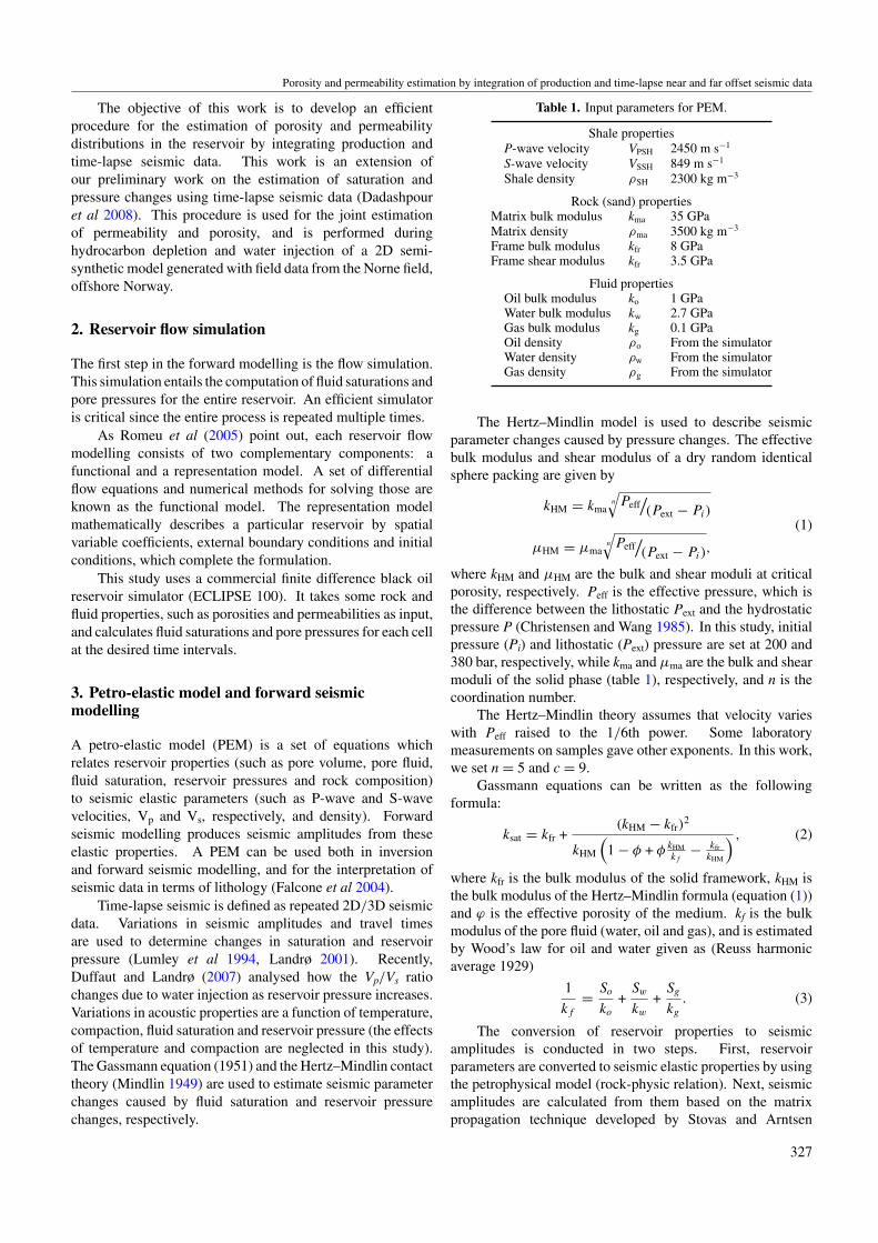
Table 1. Input parameters for PEM.

Shale propertiesP-wave velocity VPSH 2450 m s−1

S-wave velocity VSSH 849 m s−1

Shale density ρSH 2300 kg m−3

Rock (sand) propertiesMatrix bulk modulus kma 35 GPaMatrix density ρma 3500 kg m−3

Frame bulk modulus kfr 8 GPaFrame shear modulus kfr 3.5 GPa

Fluid propertiesOil bulk modulus ko 1 GPaWater bulk modulus kw 2.7 GPaGas bulk modulus kg 0.1 GPaOil density ρo From the simulatorWater density ρw From the simulatorGas density ρg From the simulator

The Hertz–Mindlin model is used to describe seismicparameter changes caused by pressure changes. The effectivebulk modulus and shear modulus of a dry random identicalsphere packing are given by

kHM = kman

√Peff

/(Pext − Pi)

μHM = μman

√Peff

/(Pext − Pi)

,

(1)

where kHM and μHM are the bulk and shear moduli at criticalporosity, respectively. Peff is the effective pressure, which isthe difference between the lithostatic Pext and the hydrostaticpressure P (Christensen and Wang 1985). In this study, initialpressure (Pi) and lithostatic (Pext) pressure are set at 200 and380 bar, respectively, while kma and μma are the bulk and shearmoduli of the solid phase (table 1), respectively, and n is thecoordination number.

The Hertz–Mindlin theory assumes that velocity varieswith Peff raised to the 1/6th power. Some laboratorymeasurements on samples gave other exponents. In this work,we set n = 5 and c = 9.

Gassmann equations can be written as the followingformula:

ksat = kfr +(kHM − kfr)

2

kHM

(1 − φ + φ kHM

kf− kfr

kHM

) , (2)

where kfr is the bulk modulus of the solid framework, kHM isthe bulk modulus of the Hertz–Mindlin formula (equation (1))and ϕ is the effective porosity of the medium. kf is the bulkmodulus of the pore fluid (water, oil and gas), and is estimatedby Wood’s law for oil and water given as (Reuss harmonicaverage 1929)

1

kf

= So

ko

+Sw

kw

+Sg

kg

. (3)

The conversion of reservoir properties to seismicamplitudes is conducted in two steps. First, reservoirparameters are converted to seismic elastic properties by usingthe petrophysical model (rock-physic relation). Next, seismicamplitudes are calculated from them based on the matrixpropagation technique developed by Stovas and Arntsen

327

M Dadashpour et al

(2006). We have used the Ricker wavelet with a centralfrequency of 30 Hz. Table 1 illustrates the input parametersfor the PEM.

4. Computer aided history matching

History matching is the calibration or conditioning of reservoirsimulation models with respect to historical production orsurvey. It is mathematically formulated by reducing the misfitbetween historical and simulated data. History matchingis usually a problem with multiple solutions, and since itrequires numerous model runs, it is normally a very expensiveprocedure.

Reservoir parameter estimation is a direct application ofthe history matching process. Every parameter estimationmethod consists of three parts:

(1) a mathematical model,(2) an objective function based on the mathematical model,(3) a minimization algorithm.

The objective function which is used in this work is

F(θ) = ‖MP (θ) − MP (θ∗)‖ + ‖MS(θ) − MS(θ∗)‖, (4)

where θ is the vector of the unknown reservoir modelparameters, MP(θ ) and MS(θ ) are the vectors of simulatedreservoir production histories and time-lapse seismicdifferences, respectively and MP(θ∗) and MS(θ∗) are thevectors of observed production historical data and time-lapseseismic differences, respectively.

In our study, the vector of unknown reservoir modelparameters includes porosity and permeability for all activecells. The MP(θ∗) vector includes well bottom hole pressuresfor both injectors and producers (WBHPI and WBHPP,respectively), and well oil and water production rates (WOPRand WWPR, respectively). The MS(θ∗) vectors includeboth time-lapse zero offset amplitudes and AVO gradientdifferences.

The Gauss–Newton algorithm is an iterative methodregularly used in solving nonlinear least-squares problems.It requires the single (Jacobin,∇F(θ)) and doubledifferentiations (Hessian,∇2F(θ)) of the objective function(equation (4)) which are usually performed numerically.The Jacobian matrix for the problem is ∇F(θ) = Jij =∂(MP (θ) + MS(θ))/∂θ , where i runs over data space and j runsover model space. For special problems, it would be useful toanalytically determine equations for these differentiations, butthese are not generally performed. Numerical differentiationrequires the calculation of the steepest descent direction andrelative step size. This procedure consists of a sequence oflinear least-squares approximations to the nonlinear problem,each of which is solved by an ‘inner’ direct or iterative process.The program needs a criterion to decide when it has convergedon the solution and it is time to stop.

The procedure is as follows (Bartholomew-Biggs 2005):

(1) choose θ0 as an estimate of θ∗,(2) repeat for k = 0, 1, 2, . . . ,(3) set fk = the vector with elements fi(θ k),(4) set Jk as the corresponding Jacobin,

(5) obtain δθ k by solving (JkTJk) δθ k = -Jk

T fk,(6) set θ k+1 = θ k +δθ k,(7) until ‖ Jk

T fk ‖ is sufficiently small.

The vector δθ k used in this algorithm approximates theNewton direction since 2Jk

Tfk = ∇F(θ)and 2JkTJk = ∇2F(θ).

Helgesen and Landrø 1993 introduced two different scalingstrategies, which were tested for various values of dampingparameter:

(1) each parameter was scaled by the diagonal Hessian matrixelement,

(2) each parameter class was scaled by the average of thecorresponding diagonal Hessian matrix element.

We used the first method, i.e. each parameter is scaledindependently by the diagonal Hessian matrix elements inorder to speed up the algorithm. The scaling is then

Hij = Hij√γiγj

Gi = Gi√γi

γi = Hii γj = Hjj ,

(5)

where H is the Hessian matrix and is defined as JkTJk, and G

is the gradient matrix which is defined as JkTfk. The sign ‘ˆ’

denotes the scaled parameters.The main advantage and disadvantage of this type of

nonlinear optimization algorithm is as follows:

Advantages:

• relatively efficient (direction and step size determined),• works especially well near the minimum,• does not require the evaluation of second-order derivatives

in the Hessian of the objective function.

Disadvantages:

• may become lost with poor initial estimates,• possibility of converging to a local minimum in the

objective function,• provides a single solution, despite the fact there are

multiple acceptable solutions that may be significantlydiverse,

• long computing time required to perform the gradientcalculation.

5. Synthetic test case

To test the efficiency and accuracy of the presentedoptimization approach, a complex semi-synthetic reservoir hasbeen set up. This model is two dimensional, and is based onfield data from the Norne Field in offshore Norway.

The Norne field is located in the blocks 6608/10 and6508/10 on a horst block in the southern part of the NordlandII in the Norwegian Sea. The horst block is approximately9 km × 3 km Norne Field, and has been exposed for twoperiods of rifting: in Perm and late Jurassic—early Cretaceous.During the first rifting, faulting affected a wide part of thearea. Especially normal faults, with NNE-SSW trends, arecommon from this period. The second rifting period canbe subdivided into four phases ranged in age from Late

328

Porosity and permeability estimation by integration of production and time-lapse near and far offset seismic data

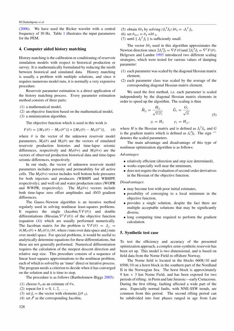
Figure 1. Stratigraphical sub-division of the Norne reservoir (Verlo and Hetland 2008).

Bathonian to Early Albian. The trend during this riftingwas footwall uplift along the Nordland Ridge, and erosion ofhigh structures. Between the two rifting periods the tectonicactivity was limited although some faulting occurred in the midand late Triassic. This period was dominated by subsidenceand transgression. The rocks within the Norne reservoirare of late Triassic to middle Jurassic age. The reservoirsandstones in the formations Tilje, Tofte, Ile and Garn aredominated by fine-grained and well- to very well sorted sub-arkosic arenites. Being buried between 2500 m and 2700m these sandstones are affected by digenetic process. Asedimentological classification of the middle Jurassic Tilje,Tofte, Ile, Not and Garn formations in the reservoir haveresulted in the definition of 14 different facies association.The deposition took place at (StatoilHydro 1998)

• a fluvial dominated coastline in a shallow seaway (lowerpart of the Tilje formation),

• a restricted lagoon (middle part of the Tilje formation),• a tidal dominated coastline in a shallow seaway

(uppermost part of the Tilje formation),

• a delta front on a fan-delta and/or a shoreline on a low-energy coast (Tofte and Ile formation),

• an open marine shoreline on a high energy coast (Not andGarn formation).

5.1. Reservoir model description

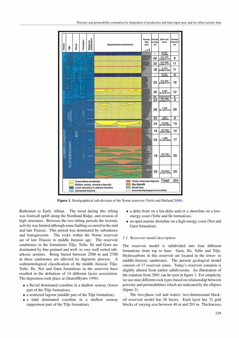
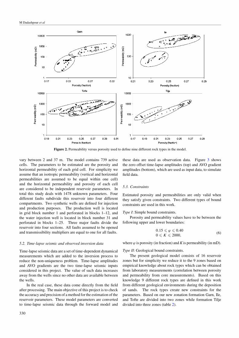
The reservoir model is subdivided into four differentformations from top to base: Garn, Ile, Tofte and Tilje.Hydrocarbons in this reservoir are located in the lower- tomiddle-Jurassic sandstones. The present geological modelconsists of 17 reservoir zones. Today’s reservoir zonation isslightly altered from earlier subdivisions. An illustration ofthe zonation from 2001 can be seen in figure 1. For simplicitywe use nine different rock types based on relationship betweenporosity and permeabilities which are indicated by the ellipses(figure 2).

The two-phase (oil and water), two-dimensional black-oil reservoir model has 26 layers. Each layer has 31 gridblocks of varying size between 48 m and 203 m. Thicknesses

329

M Dadashpour et al

Figure 2. Permeability versus porosity used to define nine different rock types in the model.

vary between 2 and 37 m. The model contains 739 activecells. The parameters to be estimated are the porosity andhorizontal permeability of each grid cell. For simplicity weassume that an isotropic permeability (vertical and horizontalpermeabilities are assumed to be equal within one cell)and the horizontal permeability and porosity of each cellare considered to be independent reservoir parameters. Intotal this study deals with 1478 unknown parameters. Fourdifferent faults subdivide this reservoir into four differentcompartments. Two synthetic wells are defined for injectionand production purposes. The production well is locatedin grid block number 1 and perforated in blocks 1–12, andthe water injection well is located in block number 31 andperforated in blocks 1–25. Three major faults divide thereservoir into four sections. All faults assumed to be openedand transmissibility multipliers are equal to one for all faults.

5.2. Time-lapse seismic and observed inversion data

Time-lapse seismic data are a set of time-dependent dynamicalmeasurements which are added to the inversion process toreduce the non-uniqueness problem. Time-lapse amplitudesand AVO gradients are the two time-lapse seismic inputsconsidered in this project. The value of such data increasesaway from the wells since no other data are available betweenthe wells.

In the real case, these data come directly from the fieldafter processing. The main objective of this project is to checkthe accuracy and precision of a method for the estimation of thereservoir parameters. These model parameters are convertedto time-lapse seismic data through the forward model and

these data are used as observation data. Figure 3 showsthe zero offset time-lapse amplitudes (top) and AVO gradientamplitudes (bottom), which are used as input data, to simulatefield data.

5.3. Constraints

Estimated porosity and permeabilities are only valid whenthey satisfy given constraints. Two different types of boundconstraints are used in this work.

Type I: Simple bound constraints.Porosity and permeability values have to be between the

following upper and lower boundaries:

0.15 � ϕ � 0.400 � K � 2000,

(6)

where ϕ is porosity (in fraction) and K is permeability (in mD).

Type II: Geological bound constraints.The present geological model consists of 16 reservoir

zones but for simplicity we reduce it to the 9 zones based onempirical knowledge about rock types which can be obtainedfrom laboratory measurements (correlation between porosityand permeability from core measurements). Based on thisknowledge 9 different rock types are defined in this workfrom different geological environments during the depositionof sands. The rock types create new constraints for theparameters. Based on our new zonation formation Garn, Ile,and Tofte are divided into two zones while formation Tiljedivided into three zones (table 2).

330

Porosity and permeability estimation by integration of production and time-lapse near and far offset seismic data

Figure 3. Observed time-lapse seismic zero offset amplitude (top)and AVO gradient (bottom).

Table 2. Geological bound constraints (type II)

Rock Limitation for Limitation forFormation type porosity (fraction) permeability (mD)

Garn 1 0.22 � φ � 0.32 150 � K � 11002 0.19 � φ � 0.24 5 � K � 110

Ile 1 0.22 � φ � 0.25 40 � K � 1502 0.22 � φ � 0.29 280 � K � 870

Tofte 1 0.20 � φ � 0.31 70 � K � 15702 0.19 � φ � 0.29 150 � K � 1950

Tilje 1 0.18 � φ � 0.26 10 � K � 7002 0.17 � φ � 0.22 40 � K � 3203 0.25 � φ � 0.27 730 � K � 2000

5.4. Sensitivity of time-lapse amplitude change to porosityand permeability

The study of the effect of reservoir parameter changes onseismic amplitude is vital to the parameter estimation problem.The sensitivity analysis is performed in this way:

(1) perturb reservoir parameters(porosity and permeability),(2) run reservoir simulation to compute saturation and

pressure at two different times (base and monitor seismicsurveys),

(3) calculate the reflection amplitudes at these two differenttimes by using petro-elastic model and forward seismicmodels,

(4) compute the amplitude changes by subtracting the resultsof the two computations,

(5) the ratios of the change in the differential amplitude to thechange in porosity and permeability provide the numericalsensitivities.

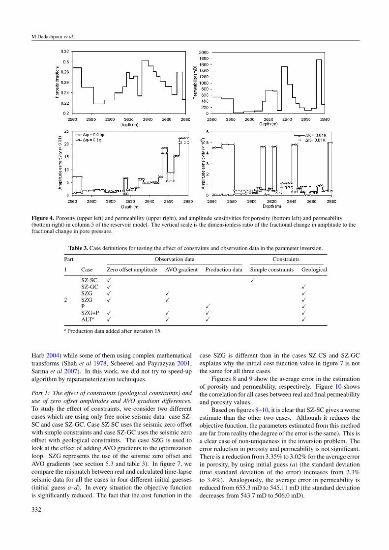
Figure 4 shows the time-lapse amplitude sensitivity withrespect to porosity and permeability in the fifth column ofthe reservoir. The amount of perturbation is representedas DELTA in the figure. There is a direct relationshipbetween permeability and porosity and the time-lapse seismicamplitude sensitivity. It is difficult to detect reservoirparameters for low permeable layers with low porosity dueto low amplitude sensitivity. In the figure DELTA Permand DELTA POR represent the amount of perturbation inpermeability and porosity, respectively. In this study, thedegree of perturbation has a significant effect on permeability,but less of an effect on porosity. A similar experiment forchanges in saturation and pressure (Dadashpour et al 2008)shows similar results.

5.5. Data matching

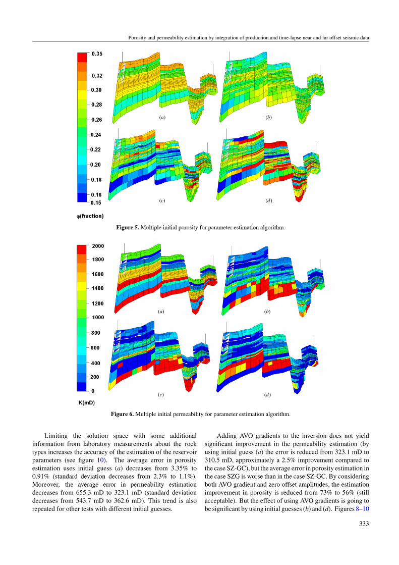
In the first part of this section, we discuss the effect of usingempirical knowledge of rock types as an inversion constraint,and we also study the use of both zero offset amplitudesand AVO gradient differences as input data in the inversion.To study the effect of noise in the inversion process twodifferent kinds of noise, white and real noise, are added tothe observation data. This study is tested with multiple initialguesses (figures 5 and 6, initial guess (a)–(d)). In the secondpart of this section we analyse the integration of productionand time-lapse seismic data in model inversion. This studyalso tested with the initial guess (a).

This type of model inversion requires an enormousnumber of forward simulations for the numericalapproximation of the gradient which made this method difficultto implement although it has a good capability to work ina distributed manner. We have implemented a distributedcomputing workflow for the estimation of reservoir propertiesfrom time-lapse seismic and production data using a Gauss–Newton optimization procedure. The case studied in thiswork has 1478 estimation parameters. It should be notedthat each forward simulation requires the numerical solutionof discretized multiphase flow equations, the calculation of theelastic parameters at each cell by rock physics equations, andfinally obtaining the seismic traces.

The computing resources are based on 20 processors froman IBM P690, 32 CPU (power-4) with 32 GB RAM under AIXversion 5.3. (using the 32 CPU was not possible due to thereduced number of flow simulation software licences). Thiswill give us a speed-up factor of approximately 20 while eachforward simulation take 26 s which 10 s is related to flowsimulation and 18 s is related to the calculation of seismicamplitudes and AVO gradients.

There are many different methods to speed-up these kindsof algorithms. One method is to reduce the order of estimatedparameters which is done in several ways. Some of thesemethods are using simple zonation techniques (Brun et al 2001,

331

M Dadashpour et al

Figure 4. Porosity (upper left) and permeability (upper right), and amplitude sensitivities for porosity (bottom left) and permeability(bottom right) in column 5 of the reservoir model. The vertical scale is the dimensionless ratio of the fractional change in amplitude to thefractional change in pore pressure.

Table 3. Case definitions for testing the effect of constraints and observation data in the parameter inversion.

Part Observation data Constraints

1 Case Zero offset amplitude AVO gradient Production data Simple constraints Geological

SZ-SC � �SZ-GC � �SZG � � �

2 SZG � � �P � �SZG+P � � � �ALTa � � � �

a Production data added after iteration 15.

Harb 2004) while some of them using complex mathematicaltransforms (Shah et al 1978, Scheevel and Payrazyan 2001,Sarma et al 2007). In this work, we did not try to speed-upalgorithm by reparameterization techniques.

Part 1: The effect of constraints (geological constraints) anduse of zero offset amplitudes and AVO gradient differences.To study the effect of constraints, we consider two differentcases which are using only free noise seismic data: case SZ-SC and case SZ-GC. Case SZ-SC uses the seismic zero offsetwith simple constraints and case SZ-GC uses the seismic zerooffset with geological constraints. The case SZG is used tolook at the effect of adding AVO gradients to the optimizationloop. SZG represents the use of the seismic zero offset andAVO gradients (see section 5.3 and table 3). In figure 7, wecompare the mismatch between real and calculated time-lapseseismic data for all the cases in four different initial guesses(initial guess a–d). In every situation the objective functionis significantly reduced. The fact that the cost function in the

case SZG is different than in the cases SZ-CS and SZ-GCexplains why the initial cost function value in figure 7 is notthe same for all three cases.

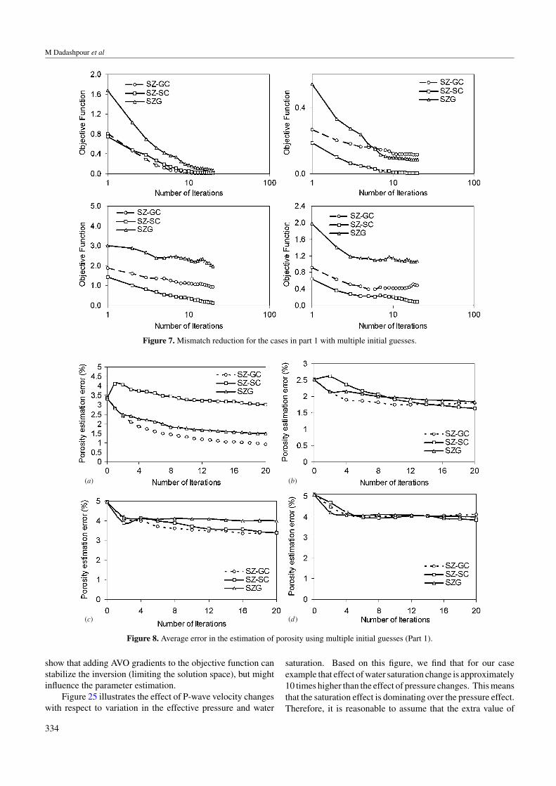
Figures 8 and 9 show the average error in the estimationof porosity and permeability, respectively. Figure 10 showsthe correlation for all cases between real and final permeabilityand porosity values.

Based on figures 8–10, it is clear that SZ-SC gives a worseestimate than the other two cases. Although it reduces theobjective function, the parameters estimated from this methodare far from reality (the degree of the error is the same). This isa clear case of non-uniqueness in the inversion problem. Theerror reduction in porosity and permeability is not significant.There is a reduction from 3.35% to 3.02% for the average errorin porosity, by using initial guess (a) (the standard deviation(true standard deviation of the error) increases from 2.3%to 3.4%). Analogously, the average error in permeability isreduced from 655.3 mD to 545.11 mD (the standard deviationdecreases from 543.7 mD to 506.0 mD).

332

Porosity and permeability estimation by integration of production and time-lapse near and far offset seismic data

(a) (b)

(c) (d)

Figure 5. Multiple initial porosity for parameter estimation algorithm.

(a) (b)

(c) (d)

Figure 6. Multiple initial permeability for parameter estimation algorithm.

Limiting the solution space with some additionalinformation from laboratory measurements about the rocktypes increases the accuracy of the estimation of the reservoirparameters (see figure 10). The average error in porosityestimation uses initial guess (a) decreases from 3.35% to0.91% (standard deviation decreases from 2.3% to 1.1%).Moreover, the average error in permeability estimationdecreases from 655.3 mD to 323.1 mD (standard deviationdecreases from 543.7 mD to 362.6 mD). This trend is alsorepeated for other tests with different initial guesses.

Adding AVO gradients to the inversion does not yieldsignificant improvement in the permeability estimation (byusing initial guess (a) the error is reduced from 323.1 mD to310.5 mD, approximately a 2.5% improvement compared tothe case SZ-GC), but the average error in porosity estimation inthe case SZG is worse than in the case SZ-GC. By consideringboth AVO gradient and zero offset amplitudes, the estimationimprovement in porosity is reduced from 73% to 56% (stillacceptable). But the effect of using AVO gradients is going tobe significant by using initial guesses (b) and (d). Figures 8–10

333

M Dadashpour et al

Figure 7. Mismatch reduction for the cases in part 1 with multiple initial guesses.

(a) (b)

(c) (d)

Figure 8. Average error in the estimation of porosity using multiple initial guesses (Part 1).

show that adding AVO gradients to the objective function canstabilize the inversion (limiting the solution space), but mightinfluence the parameter estimation.

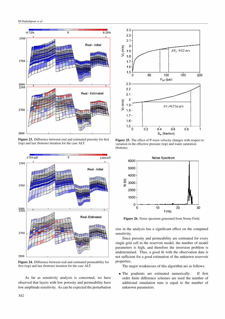
Figure 25 illustrates the effect of P-wave velocity changeswith respect to variation in the effective pressure and water

saturation. Based on this figure, we find that for our caseexample that effect of water saturation change is approximately10 times higher than the effect of pressure changes. This meansthat the saturation effect is dominating over the pressure effect.Therefore, it is reasonable to assume that the extra value of

334

Porosity and permeability estimation by integration of production and time-lapse near and far offset seismic data

(a) (b)

(c) (d)

Figure 9. Average error in the estimation of permeability using multiple initial guesses (Part 1).

(a) (b)

(c) (d)

Figure 10. Correlation between real and estimated porosity and permeability (initial guess (a)). (a) initial, (b) SZ-SC, (c) SZ-GC, (d) SZG.

using AVO data (as proposed by Landrø 2001) is somewhatlimited. Tables 4 and 5 summarize the results for all cases withmultiple initial guesses.

To check the effect of noise in the algorithm two differentkinds of noise are added to the observation data: white randomnoise which is a Gaussian distribution with no time andspatial correlation and real noise which is generated based onnoise spectrum from real 4D seismic data in the Norne field.

The amplitude spectrum was computed for several seismictraces from the Norne field. The separation between thesignal and the noise spectrum was performed by estimatingnoise by doing the following operation: rj (t) = rj (t) −(rj−1(t) + rj+1(t))/2. Then we compute Nj(ω) = FT (rj (t))

(see figure 25). The amplitude spectra for the noise averagedand used to produce the ‘colour’ noise data. The signal to noiseratio is defined as the RMS value of the signal divided by RMS

335

M Dadashpour et al

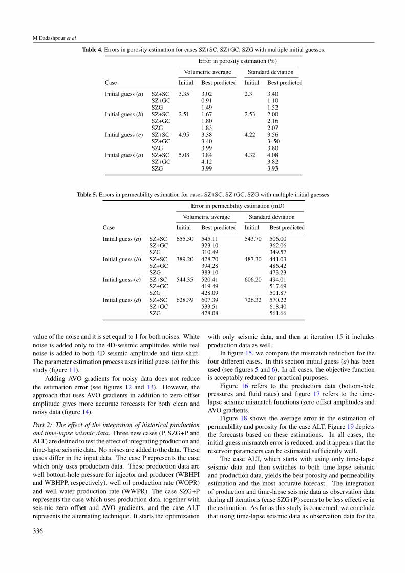
Table 4. Errors in porosity estimation for cases SZ+SC, SZ+GC, SZG with multiple initial guesses.

Error in porosity estimation (%)

Volumetric average Standard deviation

Case Initial Best predicted Initial Best predicted

Initial guess (a) SZ+SC 3.35 3.02 2.3 3.40SZ+GC 0.91 1.10SZG 1.49 1.52

Initial guess (b) SZ+SC 2.51 1.67 2.53 2.00SZ+GC 1.80 2.16SZG 1.83 2.07

Initial guess (c) SZ+SC 4.95 3.38 4.22 3.56SZ+GC 3.40 3–50SZG 3.99 3.80

Initial guess (d) SZ+SC 5.08 3.84 4.32 4.08SZ+GC 4.12 3.82SZG 3.99 3.93

Table 5. Errors in permeability estimation for cases SZ+SC, SZ+GC, SZG with multiple initial guesses.

Error in permeability estimation (mD)

Volumetric average Standard deviation

Case Initial Best predicted Initial Best predicted

Initial guess (a) SZ+SC 655.30 545.11 543.70 506.00SZ+GC 323.10 362.06SZG 310.49 349.57

Initial guess (b) SZ+SC 389.20 428.70 487.30 441.03SZ+GC 394.28 486.42SZG 383.10 473.23

Initial guess (c) SZ+SC 544.35 520.41 606.20 494.01SZ+GC 419.49 517.69SZG 428.09 501.87

Initial guess (d) SZ+SC 628.39 607.39 726.32 570.22SZ+GC 533.51 618.40SZG 428.08 561.66

value of the noise and it is set equal to 1 for both noises. Whitenoise is added only to the 4D-seismic amplitudes while realnoise is added to both 4D seismic amplitude and time shift.The parameter estimation process uses initial guess (a) for thisstudy (figure 11).

Adding AVO gradients for noisy data does not reducethe estimation error (see figures 12 and 13). However, theapproach that uses AVO gradients in addition to zero offsetamplitude gives more accurate forecasts for both clean andnoisy data (figure 14).

Part 2: The effect of the integration of historical productionand time-lapse seismic data. Three new cases (P, SZG+P andALT) are defined to test the effect of integrating production andtime-lapse seismic data. No noises are added to the data. Thesecases differ in the input data. The case P represents the casewhich only uses production data. These production data arewell bottom-hole pressure for injector and producer (WBHPIand WBHPP, respectively), well oil production rate (WOPR)and well water production rate (WWPR). The case SZG+Prepresents the case which uses production data, together withseismic zero offset and AVO gradients, and the case ALTrepresents the alternating technique. It starts the optimization

with only seismic data, and then at iteration 15 it includesproduction data as well.

In figure 15, we compare the mismatch reduction for thefour different cases. In this section initial guess (a) has beenused (see figures 5 and 6). In all cases, the objective functionis acceptably reduced for practical purposes.

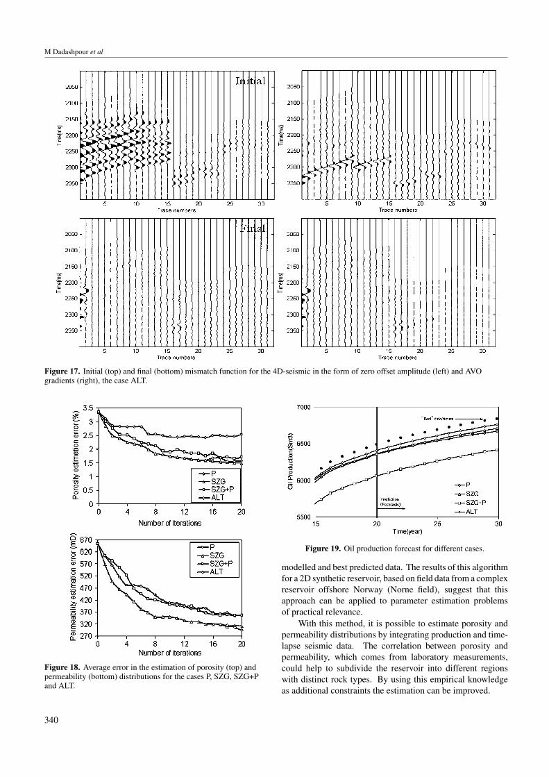
Figure 16 refers to the production data (bottom-holepressures and fluid rates) and figure 17 refers to the time-lapse seismic mismatch functions (zero offset amplitudes andAVO gradients.

Figure 18 shows the average error in the estimation ofpermeability and porosity for the case ALT. Figure 19 depictsthe forecasts based on these estimations. In all cases, theinitial guess mismatch error is reduced, and it appears that thereservoir parameters can be estimated sufficiently well.

The case ALT, which starts with using only time-lapseseismic data and then switches to both time-lapse seismicand production data, yields the best porosity and permeabilityestimation and the most accurate forecast. The integrationof production and time-lapse seismic data as observation dataduring all iterations (case SZG+P) seems to be less effective inthe estimation. As far as this study is concerned, we concludethat using time-lapse seismic data as observation data for the

336

Porosity and permeability estimation by integration of production and time-lapse near and far offset seismic data

Figure 11. White (left) and real (right) noise added to the observed zero offset amplitudes (top) and AVO gradients (bottom).

Figure 12. Mismatch reduction for the cases of noisy data using initial guess (a) (100% Gaussian noise added (left) and real noise added(right)). Dashed line indicates the misfit of the true solution.

permeability and porosity estimation gives better results thanonly considering production historical data.

In the case ALT, the average error in the estimationof porosity decreases from 3.35% to 1.58% (the standarddeviation decreases from 2.3% to 1.52%), and in the estimationof permeability from 655.29 mD to 294.45 mD (the standarddeviation decreases from 543.7 mD to 333.1 mD).

Average errors (for cases SZP, P, SZP+P and ALT) inthe estimation of porosity and permeability are summarized intables 6 and 7, respectively.

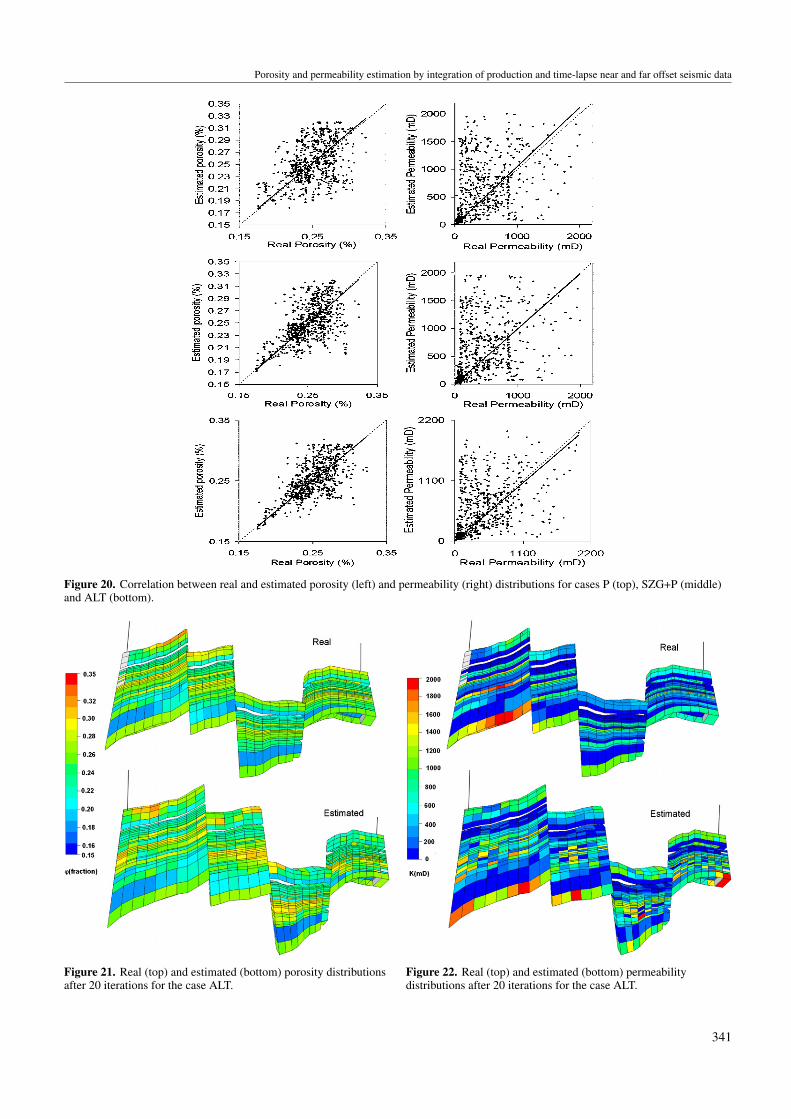
In figure 20, we compare the correlation for cases P,SZP+P and ALT between real and estimated porosity andpermeability distributions. Figures 21 and 22 represent realand estimated porosity and permeability distributions for thecase ALT.

Figures 23 and 24 show the error in the estimation ofporosity and permeability in the first and last iterations for thecase ALT. We can see in these figures how the error in theinitial guess is reduced.

337

M Dadashpour et al

Figure 13. Average error in the estimation of porosity (top) and permeability (bottom) in the noisy data using initial guess (a) (100%Gaussian noise added (left) and real noise added (right)).

Figure 14. Oil production forecast for different cases Part 1 without noise (top-left), with white noise (top-right) and real noise (bottom).

This parameter estimation problem is underdetermined,which explains that adding extra information in the algorithmfor limiting the solution space has a positive effect in improvingthe estimation process. The main difficulties in this problemcan be attributed to two thin highly permeable layers (see

figure 22, layers 13 and 20) and to an area close to the injectionwell. It is very difficult to detect thin highly permeablezones by seismic methods since seismic has limited verticalresolution. Therefore, the algorithm tends to spread theestimation in the vertical direction. In this study, we detect

338

Porosity and permeability estimation by integration of production and time-lapse near and far offset seismic data

Table 6. Errors in porosity estimation for cases SZG, P, SZG+P andALT.

Error in porosity estimation (%)

Volumetric average Standard deviation

Case Initial Best predicted Initial Best predicted

SZG 3.35 1.49 2.3 1.52P 2.54 1.96SZG+P 1.73 1.63ALT 1.58 1.52

Table 7. Errors in permeability estimation for cases SZG, P, SZG+Pand ALT.

Error in permeability estimation (mD)

Volumetric average Standard deviation

Case Initial Best predicted Initial Best predicted

SZG 655.3 310.5 543.7 349.6P 355.3 374.0SZG+P 356.7 371.6ALT 294.4 331.1

some layers with medium permeability instead of just twowith high permeability. A more accurate bound constraintselection in problematic zones, as those described, can bebeneficial in the estimation. In any case, including geological

Figure 16. Best predicted, historical and initial values for the case ALT concerning the well bottom-hole pressure in the injector (left top)and in the producer (left bottom), and the well oil production (right top) and water production rates (right bottom).

Figure 15. Mismatch reduction for the cases in Part 2.

information in the process is, according to the results presentedhere, indispensable.

6. Discussion

In this paper we have introduced a systematic approachfor estimating reservoir parameters such as porosity andpermeability by integrating production and time-lapse seismicdata in the form of zero offset amplitudes and AVO gradientdifferences. This methodology is based on the Gauss–Newtonoptimization technique for reducing the mismatch between

339

M Dadashpour et al

Figure 17. Initial (top) and final (bottom) mismatch function for the 4D-seismic in the form of zero offset amplitude (left) and AVOgradients (right), the case ALT.

Figure 18. Average error in the estimation of porosity (top) andpermeability (bottom) distributions for the cases P, SZG, SZG+Pand ALT.

Figure 19. Oil production forecast for different cases.

modelled and best predicted data. The results of this algorithmfor a 2D synthetic reservoir, based on field data from a complexreservoir offshore Norway (Norne field), suggest that thisapproach can be applied to parameter estimation problemsof practical relevance.

With this method, it is possible to estimate porosity andpermeability distributions by integrating production and time-lapse seismic data. The correlation between porosity andpermeability, which comes from laboratory measurements,could help to subdivide the reservoir into different regionswith distinct rock types. By using this empirical knowledgeas additional constraints the estimation can be improved.

340

Porosity and permeability estimation by integration of production and time-lapse near and far offset seismic data

Figure 20. Correlation between real and estimated porosity (left) and permeability (right) distributions for cases P (top), SZG+P (middle)and ALT (bottom).

Figure 21. Real (top) and estimated (bottom) porosity distributionsafter 20 iterations for the case ALT.

Figure 22. Real (top) and estimated (bottom) permeabilitydistributions after 20 iterations for the case ALT.

341

M Dadashpour et al

Figure 23. Difference between real and estimated porosity for first(top) and last (bottom) iteration for the case ALT.

Figure 24. Difference between real and estimated permeability forfirst (top) and last (bottom) iteration for the case ALT.

As far as sensitivity analysis is concerned, we haveobserved that layers with low porosity and permeability havelow amplitude sensitivity. As can be expected the perturbation

Figure 25. The effect of P-wave velocity changes with respect tovariation in the effective pressure (top) and water saturation(bottom).

Figure 26. Noise spectrum generated from Norne Field.

size in the analysis has a significant effect on the computedsensitivity.

Since porosity and permeability are estimated for everysingle grid cell in the reservoir model, the number of modelparameters is high, and therefore the inversion problem isundetermined. Thus, a good fit with the observation data isnot sufficient for a good estimation of the unknown reservoirproperties.

The major weaknesses of this algorithm are as follows.

• The gradients are estimated numerically. If firstorder finite difference schemes are used the number ofadditional simulation runs is equal to the number ofunknown parameters.

342

Porosity and permeability estimation by integration of production and time-lapse near and far offset seismic data

• As in any local optimization algorithm, there is a strongdependency on the initial guess taken.

• It is not straight forward to find constraints that properlylimit the solution space.

This approach is suitable for distributed computing andfor time demanding forward models (in this case the gradientestimation will be accelerated considerably). A distributedcomputing optimization framework is developed and appliedsuccessfully.

The main advantage of this method with respect to theother optimization techniques are right descent direction, theprocedure converges quadratically at the optimal point, noneed to compute second derivative of objective function forcomputing Hessian matrix and it requires less simulation runwith respect to global optimizers like genetic algorithm.

Future work is to increase the speed of the optimization.One method is reducing the number of parameters whichis called reparameterization (Dadashpour et al 2009).Reparameterization can be done by simple zonation orby mathematical transforms techniques. We will tryto use gradzone and principal component analysis whichincorporated in a distributed computing environment to speedup the parameter estimation. We hope that with using thesetechniques it will be possible to use these types of optimizationin the large and realistic problems.

7. Conclusions

A Gauss–Newton optimization technique is used to estimateporosity and permeability distributions. This algorithm isconditioned to production and time-lapse near and far offsetdata. The result shows that AVO gradient can increase thestability of the parameter estimation. Empirical knowledgeabout rock types can improve the estimation by means of someadditional constraints in the optimization routine. Increasingthe sensitivity of amplitudes to the estimated parameters canincrease the accuracy of the estimates.

Integrating production history and time-lapse seismic dataas observation data is better implemented in two steps:

(1) limiting the solution space by only using time-lapseseismic data,

(2) after a number of optimization iterations, consider bothproduction history and time-lapse seismic data in themisfit function.

In this study we have observed that using only time-lapseseismic data is more effective for permeability and porosityestimation than using only production performance historicaldata.

It is very difficult to detect thin high permeable zones byseismic methods. This is probably associated with less verticalresolution in the seismic data.

Distributed computing can significantly accelerate theparameter estimation process.

Acknowledgments

The authors want to thank the Norwegian University of Scienceand Technology (NTNU), the Research Council of Norway(NFR) and TOTAL for financial support. The authors wishto gratefully acknowledge StatoilHydro for permitting theutilization of the reservoir model. We also want to thankSchlumberger-GeoQuest for the use of the simulator ECLIPSEand Alexey Stovas for preparing the seismic forward model.Lastly, we would like to extend our gratitude to Jan Ivar Jensen,Knut Backe and Erlend Våtevik from NTNU for their helpduring this study.

References

Aanonsen S I, Aavatsmark I, Barkve T, Cominelli A, Gonard R,Gosselin O, Kolasinski M and Reme H 2003 Effect of scaledependent data correlations in an integrated history matchingloop combining production data and 4d seismic data, SPE79665 SPE Reservoir Simulation Symp. (Houston, USA,3–5 February)

Arenas E, Kruijsdijk C and Oldenziel T 2001 Semi-automatichistory matching using the pilot point method includingtime-lapse seismic data, SPE 71634 SPE Annual TechnicalConf. and Exhibition (New Orleans, USA,30 September–3October)

Bartholomew-Biggs M 2005 Nonlinear Optimization with FinancialApplications (Dordrecht: Kluwer/Academic)

Behrens R, Condon P, Haworth W, Bergeron M, Wang Z andEcker C 2002 4D seismic monitoring of water influx at BayMarchand: the practical use of time-lapse in an imperfectworld SPE Reservoir Eval. Eng. 5 410–20

Brun B, Gosselin O and Barker J W 2001 Use of prior informationin gradient-based history-matching, SPE 66353 SPE ReservoirSimulation Symp. (Texas, USA,11–14 February)

Burianyk M 2000 Amplitude-vs-Offset and seismic rock propertyanalysis: a primer CSEG Recorder Calgary

Burkhart T, Hoover A R and Flemings P B 2000 Time-lapse (4-D)seismic monitoring of primary production of turbiditereservoirs as South Timbalier Block 295, offshore Louisiana,Gulf of Mexico Geophysics 65 351–67

Christensen N I and Wang H F 1985 The influence of pore pressureand confining pressure on dynamic elastic properties of Bereasandstone Geophysics 50 207–13

Chu L, Reynolds A C and Oliver D S 1995 Computation ofsensitivity coefficients for conditioning the permeability fieldto well-test pressure data In Situ 19 179–223

Dadashpour M, Echeverria C D, Mukerji T, Kleppe J and Landrø M2009 Simple zonation and principal component analysis forspeeding-up porosity and permeability estimation from 4Dseismic and production data, extended abstract 71st EAGEConf. and Exhibition Incorporating SPE EUROPEC(Amsterdam, 8–11 June)

Dadashpour M, Landrø M and Kleppe J 2008 Non-linear inversionfor estimating reservoir parameters from time-lapse seismicdata J. Geophys. Eng. 5 54–66

Dong Y and Oliver D S 2005 Quantitative use of time-lapse seismicdata for reservoir description, SPE 84571 SPE J. 10 91–9

Duffaut K and Landrø M 2007 Vp/Vs ratio versus differential stressand rock consolidation—a comparison between rock modelsand time-lapse AVO data Geophysics 5 81–94

Eastwood J, Lebel J P, Dilay A and Blakeslee S 1994 Seismicmonitoring of steam-based recovery of bitumen The LeadingEdge 4 242–51

Falcone G, Gosselin O, Maire F, Marrauld J and Zhakupov M 2004Petroelastic modelling as key element of 4D history matching:

343

M Dadashpour et al

a field example, SPE 90466 SPE Annual Technical Conf. andExhibition, (Houston, USA, 26–29 September,)

Furre A K, Munkvold F R and Nordby L H 2003 Improvingreservoir understanding using time-lapse seismic at theHeidrun field 65th Mtg., Eur. Assn. Geosci. Eng., A20

Gassmann F 1951 Elastic wave through a packing of spheresGeophys. J. 16 673–85

Gosselin O, Aanonsen S I, Aavatsmarka I, Cominelli A, Gonard R,Kolasinski M, Ferdinandi F, Kovacic L and Neylon K 2003History matching using time-lapse seismic (HUTS), SPE 84464SPE Reservoir Simulation Symp (Denver, USA, 5–8 October)

Greaves R J and Fulp T J 1987 Three-dimensional seismicmonitoring of an enhanced oil recovery processGeophysics 52 1175–87

Harb R 2004 History matching including 4-D seismic—anapplication to a field in the North Sea Master Thesis, NTNUNorway

Haskell N A 1953 The dispersion of surface waves in multilayeredmedia Bull. Seismol. Soc. Am. 43 17–34

Helgesen J and Landrø M 1993 Estimation of elastic parametersfrom AVO effects in the tau-p domain Geophys.Prospect. 41 341–66

Huang X, Meister L and Workman R 1997 Reservoircharacterization by integration of time-lapse seismic andproduction data, SPE 38695 SPE Annual Technical Conf. andExhibition (San Antonio, USA, 5–8 October)

Huang X, Will R and Waggoner J 2000 Reconciliation of time-lapseseismic data with production data for reservoir management: aGulf of Mexico Reservoir, SPE 65155 SPE EuropeanPetroleum Conference (Paris, France, 24–25 October)

Jacquard P and Jain C 1965 Permeability distribution from fieldpressure data Soc. Pet. Eng. J., Trans., AIME 234 281

Kennett B L N 1983 Seismic Wave Propagation in Stratified Media(Cambridge UK: Cambridge University Press) p 342

Koster K, Gabriels P, Hartung M, Verbeek J, Deinum G and StaplesR 2000 Time-lapse seismic surveys in the North Sea and theirbusiness impact The Leading Edge 19 286–93

Landa J L and Horne R N 1997 Procedure to integrate well test data,reservoir performance history and 4-D seismic information intoa reservoir description, SPE 38653 Annual Technical Conf. andExhibition (San Antonio, USA, 5–8 October)

Landrø M 2001 Discrimination between pressure and fluidsaturation changes from time-lapse seismic data Geophys. J.3 66

Landrø M 2004 Seismic data acquisition and processing 65–6 Handnotes

Landrø M, Solheim O A, Hilde E, Ekren B O and Strønen L K 1999The Gullfaks 4D seismic study Pet. Geosci. 3 213–26

Lazaratos S K and Marion B P 1997 Croswell seismic imaging ofreservoir changes caused by CO2 injection The LeadingEdge 16 1300–7

Lumley D E, Nur A, Strandenes S, Dvorkin J and Packwood J 1994Seismic monitoring of oil production: a feasibility study:expanded abstracts 64th Ann. Internat. Mtg, Soc. Expl.Geophys.

Mezghani M, Fornel A, Langlais V and Lucet N 2004 Historymatching and quantitative use of 4D seismic data for animproved reservoir characterization, SPE 90420 SPE AnnualTechnical Conf. and Exhibition (Houston, USA, 26–29September)

Mindlin R D 1949 Compliance of elastic bodies in contact J. Appl.Mech. 16 259–68

Minkoff S, Labs S N, Symes W, Bryant S, Eaton J and Wheeler M1998 Reservoir characterization via time-lapse prestack seismicin version 68th Annual International Meeting of the Society ofExploration Geophysicists (New Orleans, USA) pp 44–47

Oliver D S 1996 A comparison of the value of interference andwell-test data for mapping permeability and porosity In Situ20 41–59

Reuss A 1929 Berechnung der fliessgrense von mishkristallen Z.Angew. Math. Mech. 9 49–58

Romeu R K, Paraizo P L B, Moraes M A S, Lima C C, Lopes M RF, Silva A T, Rodrigues J R P, Silva F P T, Cardoso MA andDamiani M C 2005 Reservoir representation for flowsimulation, SPE 94735 SPE Latin American and CaribbeanPetroleum Engineering Conf. (Rio de Janeiro, Brazil, 20–23June)

Sarma P, Durlofsky L and Aziz K 2007 A new approach toautomatic history matching using Kernel PCA, SPE 106176SPE Reservoir Simulation Symp. (Houston, USA, 26–28February)

Scheevel J R and Payrazyan K 2001 Principal component analysisapplied to 3D seismic data for reservoir property estimationSPE Reservoir Eval. Eng. 4 64–72

Shah P C, Gavalas G R and Seinfeld J H 1978 Error analysis inhistory matching: the optimum level of parameterization Soc.Petrol. Eng. J 18 219–28

Skorstad A, Kolbjørnsen O, Drottning A, Gjøystdal H and HusebyO 2006 Combining saturation changes and time-lapse seismicfor updating reservoir characterizations, SPE 106366 SPEReservoir Eval. Eng. 9 502–12

StatoilHydro 1998 Norne Field: Sedimentological EvaluationStephen K D, Soldo J and MacBeth C 2006 Multiple-model seismic

and production history matching: a case study, SPE 94173 SPEJ. 11 413–30

Stovas A and Arntsen B 2006 Vertical propagation of low-frequencywaves in finely layered media Geophys. J. 71 87–94

Vasco D W, Datta-Gupta A, Behrens R, Condon P and Rickett J2004 Seismic imaging of reservoir flow properties: time-lapseamplitude changes Geophys. J. 69 1425–42

Vasco D W, Datta-Gupta A and He Z 2003 Reconciling time-lapseseismic and production data using streamline models: the BayMarchand Field, Gulf of Mexico, SPE 84568 SPE AnnualTechnical Conf. and Exhibition (Denver, USA, 5–8 October )

Verlo S B and Hetland M 2008 Development of a field case with realproduction and 4D data from the Norne Field as a benchmarkcase for future reservoir simulation model testing MasterThesis, NTNU Norway

Waggoner J R, Cominelli A and Seymour R H 2002 Improvedreservoir modeling with time-lapse seismic in a Gulf of MexicoGas Condensate Reservoir, SPE 77514 SPE Annual TechnicalConf. and Exhibition (San Antonio, USA, 29 September–2October)

Walker G J and Lane H S 2007 Assessing the accuracy ofhistory-match predictions and the impact of time-lapse seismicdata: a case study for the harding reservoir, SPE 106019Reservoir Simulation Symp. (Houston, U.S.A., February 26–28)

Yannong D and Oliver D S 2005 Quantitative use of 4D seismic datafor reservoir description, SPE84571 SPE J.10 91–9

344