savings, the dwelling sector and participation rates in the...
TRANSCRIPT

..
Savings, The Dwelling Sector
and Participation Rates
in The Treasury Macroeconomic
(TRYM)
Model
By
Lawrence Antioch and Bruce Taplin
This document is based on the research and development work undertaken in recent years in the
Modelling Section of the Treasury. It has been released in the interests of making information of
this kind available to others working in the same general field and of fostering public discussion
and evaluation of the research results that are embodied in the model.
The authors would like to acknowledge the contributions of Mr Brett Ryder, Dr Barry Gray and Ms
Priya Parameswaran. However the usual caveats apply.
TRYM PAPER No. 5

2
This document is one of a series presented at the June 1993 Treasury Conference on The TRYMModel of the Australian Economy. The full set of papers presented at the conference are listedbelow.
• An Introduction to the Treasury Macroeconomic (TRYM) Model of the Australian Economy
(TRYM Paper No.1)
• Documentation of the Treasury Macroeconomic (TRYM) Model of the Australian Economy
(TRYM Paper No. 2)
• Employment, Investment and Productivity: Decisions by the Firm
(TRYM Paper No. 3)
• Exports, Imports and the Trade Balance
(TRYM Paper No. 4)
• Savings, Dwelling Investment and the Labour Market: Decisions by Households
(TRYM Paper No. 5)
• Australia's Trade Linkages with the World
(TRYM Paper No. 6)
• The Macroeconomic Effects of Higher Productivity
(TRYM Paper No. 7)

3
TABLE OF CONTENTS
INTRODUCTION................................................................................................................. 3
1.0 CONSUMPTION AND SAVING BEHAVIOUR .......................................................... 5
1.1 Data considerations.............................................................................................. 8
1.11 Private final consumption...................................................................... 8
1.12 Measurement of non-property income................................................... 8
1.13 Measurement of wealth.......................................................................... 9
1.2 Specification of the consumption equation
................................................................................................................................... 1
1
1.3 Estimation and interpretation of results
................................................................................................................................... 1
4
2.0 DWELLING SECTOR
............................................................................................................................................... 1
5
2.1 Data considerations
................................................................................................................................... 1
6
2.2 Specification of the demand for rental services
................................................................................................................................... 1
7
2.3 Estimation and interpretation of results
................................................................................................................................... 2
0

4
2.4 Specification of the supply of rental services (dwelling investment)
................................................................................................................................... 2
1
2.5 Estimation and interpretations of results
................................................................................................................................... 2
4
3.0 LABOUR SUPPLY BEHAVIOUR
............................................................................................................................................... 2
6
3.1 Data considerations
................................................................................................................................... 2
7
3.2 Specification of the labour supply equation
................................................................................................................................... 3
1
3.3 Estimation and interpretations of results
................................................................................................................................... 3
2
4.0 CONCLUSION
............................................................................................................................................... 3
4

5
INTRODUCTION
The aim of this paper is to describe how the TRYM model analyses some of the important decisions
made by households. These are the choice between consumption and saving, the level of
investment expenditure on dwellings as consumers and investors, and participation in the labour
force. These decisions are captured by four behavioural equations for private final consumption
expenditure, the price of rents, dwelling investment and labour supply.
These decisions have been modelling in a simple and transparent way using the recently rebased
National Accounts data. Our overall objective was to strike a balance between data and theoretical
considerations, which we believe we have achieved given the small amount of time available since
this new data became available.
The relationship between consumption, income and wealth is important for macroeconomic models.
Not surprisingly, we find that there is a strong causal relation between these variables, consistent
with Fisher's theory of intertemporal optimisation. We specify a general consumption equation that
encompasses a number of different theories and let the data choose the relative strengths of different
linkages.
In the dwelling sector, our objective was to explain dwelling investment in the post deregulation
period. This objective is accomplished given the restriction that our experience with a deregulated
financial market has been limited to only one complete cycle. Finally, labour supply was specified
to take account of both movements in the demand for labour and supply factors, such as
demographic and structural changes. Because we have modelled labour supply on an hours basis,
we have in broad terms, attempted to capture some part of the significant shift towards part-time
employment.
The basic structure of the household sector is as follows. Households sell labour services to the
business and government sectors and receive a wage income in exchange for their labour services.
They can also build up or run down their stock of private sector wealth. This wealth may be held in
a variety of different forms - dwellings, business assets (real and financial), public securities and
Reserve Bank liabilities. The expected rate of return from this stock of wealth provides a flow of
expected income to the household sector.
Households appear to smooth consumption spending to some extent and savings are determined as a
residual1. There are a number of factors that will influence the saving decision: the desire to smooth
1. The level of savings in the TRYM model are not directly comparable to the ABS savings measure because there aredifferences in the measurement of property incomes.

6
consumption; desire (either implicitly or explicitly) to hold a particular level of wealth; and the level
of uncertainty households experience. Government policies, such as taxes and transfer payments,
can also affect the level of savings.
Having determined the split between consumption and saving, we assume households allocate
consumption spending, in each period, between rent consumption and non-rent consumption.
Dwelling investment by households is found to depend on a comparison between rental returns and
the cost of funds and the state of the labour market.
The labour force participation decisions depend on the encouraged worker effect, real wages and
average hours worked per employed persons.
Although the specification of these equations is based on economic principles there is no unifying
theoretical framework, such as utility maximisation, that attempts to link them. This outcome
reflects a trade-off between theoretical and data considerations. The main disadvantage of a unified
utility maximisation framework is that it imposes constraints on the modelling of macro behaviour
of households that may not always be reflected in the data. For example, there are little data on
households' intertemporal discount rate and where there are data they are not available on a
consistent basis. Moreover, the TRYM model is not designed to examined the effects of changes in
microeconomic parameters that are best captured in an integrated framework. In addition, some of
the macroeconomic variables that could have provided additional linkages between different
decisions were found to have an insignificant effect on households decisions.
However, this does not imply that inter linkages between household decisions have been ignored
where they will assist our understanding of macro economic issues. There are obvious inter
linkages between some decisions, such as between the price of rents and dwelling investment
equations. These can be interpreted as representing the demand and supply curves for dwellings
respectively and are estimated jointly.
This paper is organised as follows. In section one households' consumption and saving decisions
are examined. Dwelling investment is examined in section two while labour supply decisions are
discussed in section three. In section four we draw appropriate conclusions from this work.
1.0 CONSUMPTION AND SAVING BEHAVIOUR
The relationship between consumption, income and non-human wealth has been a subject of
considerable analysis but remains an area of much controversy. There remains disagreement, for
example, on the effects of interest rates and the prevalence of borrowing constraints. Nevertheless,
these relationships form an important basis for macroeconometric models and the consumption

7
decision must be modelled even though there are some major outstanding issues (Blinder and
Deaton 1985).
In modelling households' consumption-saving decisions, most economists follow one of two ways
of implementing Fisher's theory of inter temporal optimisation; this theory allows households to
smooth consumption through borrowing and saving (lending), allowing current income to deviate
from current consumption. One strand is represented by the theoretical specifications suggested by
the work of Friedman (1957) and Ando and Modigliani (1963) in which an important determinant
of consumption is wealth.
In contrast, more recent work by Delong and Summers (1986) suggests that current income plays a
more important role, consistent with Keynes' consumption function. Our approach has been to
adopt a general specification that encompasses the main ideas expressed in the literature and to
allow the data to determine the relative ability of the competing theories to explain the
macroeconomic data over the sample period.
The basic permanent-income hypothesis, developed by Friedman, postulates that consumption
depends upon the long run average (permanent) income households expect to receive. This means
that if actual income is above (or below) permanent income households' savings will rise (or fall).
Private consumption should depend on the interest rate, the ratio of non-human wealth to permanent
income, income variability, and certain life cycle variables. It is the level of an average expected
income from wealth that is important rather than the stock of wealth. To the extent that most
variation in income is transitory, the theory suggests that consumption should be smooth.
The basic life-cycle hypothesis, on the other hand, postulates that consumers try to stabilise their
consumption over their entire life-time. This hypothesis also implies that consumption depends not
just on current income but also on the actual value of assets and liabilities of those consumers
relative to a desired level. This desired value of net private wealth is determined by a range of
microeconomic influences that are beyond the scope of this study. In the long run, the hypothesis
predicts a constant saving (or consumption) to income ratio but, in the short run, one that varies
over the business cycle. It is the stock of wealth rather than the flow of income that is important in
the determination of consumption.
A key difference between Fisher's approach and more recent research on consumption behaviour is
the role of capital markets. For households to achieve a smooth level of consumption over their
lives, they should be able to borrow as much as they wish now, on the basis that there should be
sufficient expected income to repay the loan in the future. This is generally true for young
households whose current income is low would need to borrow against expected high income in
later years to maintain a smooth consumption profile. However, financial institutions do not

8
generally allow young households to borrow all they like, with the result that at a current point of
time they could be liquidity constrained. This is a feature of an imperfect capital market. Another
is the existence of interest rate spreads between borrowing and lending rates.
The presence of imperfect capital markets suggests that current income should play a much more
important role in consumption decisions than both the permanent income and life-cycle hypotheses
imply.
Therefore, in this modelling, private consumption was specified to depend on real non-property
income, real non-human private wealth and changes in the unemployment rate and non-property
income. However, the 1980s data suggest that fluctuation in current income has less of an effect on
current consumption than it did during the 1970s. This result is consistent with the work of
Blundell-Wignall, Browne, Cavaglia and Tarditi (1992)2.
There are two issues that must also be addressed before we estimate a consumption function. The
first is whether households are forward looking. Although the permanent income and the life-cycle
theories imply forward looking behaviour, our model specification assumes that the household and
the business sectors, unlike the financial sector, are not forward looking. The information set of
households consists of current and past information only. However, the inclusion of wealth in the
consumption function suggests that there may be some forward looking information with respect to
financial market's valuation of business and financial assets. This feature of the TRYM model is
broadly consistent with other models, with the exception of the MGS model where a proportion of
consumers can be forward looking.
The second is the extent to which households consolidate their account with those of business and
government sectors. The are two extreme positions here. First, households consolidate their
accounts with those of business and government sectors, a view that is consistent with forward
looking behaviour. Alternatively, households do not consolidate such accounts, a view that is
consistent with myopic behaviour. In the TRYM model, we adopt a middle position that assumes
households fully consolidate their accounts with the business sector but not with the government
sector.
An immediate implication of this middle position is the non-fulfilment of the Ricardian Equivalence
hypothesis. The theorem states that, for a given path of government spending, a debt financed tax
cut has no real effects on the economy because consumers realise that the cut in current taxes will
lead to higher future taxes and therefore consumption will not increase (Barro 1974).
2. Hayashi (1985) also provides a critical survey of empirical work on liquidity constraints.

9
In the TRYM model, because households do not fully take account of the government's
intertemporal budget constraint, a debt financed tax cut would make households better off causing
them to increase their consumption. This means that in the TRYM model, size of government debt
will have real effects on households' behaviour and the economy's short run real equilibrium. A
fundamental feature of the model is that consumers do not anticipate the rise in taxes over the
medium to long run whereas under the Ricardian assumption the rise in taxes would be fully
anticipated.
1.1 Data considerations
1.11 Private final consumption
An important feature of the permanent income and life-cycle hypotheses is the relative stability of
consumption over the business cycle compared with other components of GDP such as labour
income. This is a feature that is also reflected in the aggregate consumption data, as evident in the
following chart.
PRIVATE FINAL CONSUMPTION EXPENDITURE AND NON-PROPERTY INCOME
25000
30000
35000
40000
45000
50000
55000
60000
Ma
r-7
0
Ma
r-7
1
Ma
r-7
2
Ma
r-7
3
Ma
r-7
4
Ma
r-7
5
Ma
r-7
6
Ma
r-7
7
Ma
r-7
8
Ma
r-7
9
Ma
r-8
0
Ma
r-8
1
Ma
r-8
2
Ma
r-8
3
Ma
r-8
4
Ma
r-8
5
Ma
r-8
6
Ma
r-8
7
Ma
r-8
8
Ma
r-8
9
Ma
r-9
0
Ma
r-9
1
Ma
r-9
2
CON Real YLZ
The TRYM model examines total private final consumption expenditure as measured in the
National Accounts; in NIF10 and NIF88 consumption was disaggregated. The option to split
consumption expenditure between durables and non-durables was considered, but not implemented
for a number of reasons; in particular, the distinction between durables and non-durables is not
always clear, and involve some measurement and definitional problems. Moreover, the aim and
focus of TRYM is to model aggregate consumption-savings behaviour and disaggregation did not
seem helpful. The approach adopted here is also consistent with the treatment of other components
10
of GDP, such as commodity exports and business investment, which have a greater claim for
disaggregation.
1.12 Measurement of non-property income
The level of non-property income (YLZ) available to households, as defined in the TRYM model,
consists of labour income and government transfers3. Labour income is the sum of wages, salaries
and supplements less PAYE taxes (net of refunds) plus an imputed income for the self employed
and employers. The employers and/or self employed are assumed to have the same after tax wage
as those paid wages and salaries. Government transfers are largely personal benefit payments but
include some other outlays, such as some payments to non profit institutions.
The TRYM definition of non-property income reflects our finding that it is difficult to obtain
statistically different marginal propensities to consume out of labour and transfer incomes.
Although we found some indication that the marginal propensity to consume from transfer income
is somewhat less than the propensity to consume from labour income, we attributed this result to
the correlation in economic downturns between higher transfer payments and greater uncertainty
which reduces consumption. Faced with these estimation difficulties, we decided to constrain these
different propensities to be the same.
1.13 Measurement of wealth
The methodology used to derive quarterly estimates of aggregate non-human private wealth is based
on Piggott (1986) and Callen (1991). However, there are some differences in methodologies that
have been outlined in the Economic Round-Up, Summer (1990) and Summer (1992) editions.
Private sector wealth in TRYM is derived as the sum of the market value of business assets (net of
foreign ownership and private sector foreign debt), dwelling capital stock, Australian equity
investment abroad, consumer durables, public securities and Reserve Bank liabilities.
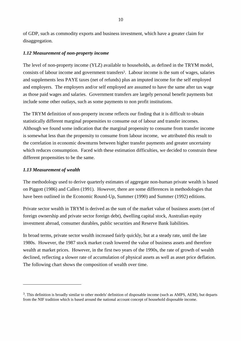
In broad terms, private sector wealth increased fairly quickly, but at a steady rate, until the late
1980s. However, the 1987 stock market crash lowered the value of business assets and therefore
wealth at market prices. However, in the first two years of the 1990s, the rate of growth of wealth
declined, reflecting a slower rate of accumulation of physical assets as well as asset price deflation.
The following chart shows the composition of wealth over time.
3. This definition is broadly similar to other models' definition of disposable income (such as AMPS, AEM), but departsfrom the NIF tradition which is based around the national account concept of household disposable income.

11
PRIVATE SECTOR WEALTH AT MARKET PRICES
0
2000
4000
6000
8000
10000
12000
14000
16000
Jun
-59
Jun
-60
Jun
-61
Jun
-62
Jun
-63
Jun
-64
Jun
-65
Jun
-66
Jun
-67
Jun
-68
Jun
-69
Jun
-70
Jun
-71
Jun
-72
Jun
-73
Jun
-74
Jun
-75
Jun
-76
Jun
-77
Jun
-78
Jun
-79
Jun
-80
Jun
-81
Jun
-82
Jun
-83
Jun
-84
Jun
-85
Jun
-86
Jun
-87
Jun
-88
Jun
-89
Jun
-90
Jun
-91
Jun
-92
Dwelling Stock Business Capital Stock Other
$m '000
Between 1960 and 1975, the composition of Australia's net private wealth shifted quite
significantly. The share of dwelling capital, for example, increased from about 35 per cent to 57 per
cent, while business capital fell from about 43 per cent to 25 per cent. Other notable composition
changes included a decline in public securities from about 11 per cent to 8 per cent, while consumer
durables fell from about 11 per cent to 8 per cent and Reserve Bank liabilities also fell from about 3
per cent to 2 per cent.
Since 1975 the composition of private sector wealth has been relatively stable, with the relative
shares of dwellings and business capital - in particular, remaining broadly unchanged. Exceptions
have been the sharp rise in Australian equity investment abroad (from 0.8 per cent to about 5 per
cent) while public sector securities continued to decline (from about 8 per cent to 6 per cent).
During 1986 and 1987 the value of private sector wealth was quite volatile; largely reflecting
movements in share prices. House prices rose fairly quickly in 1988. An interesting feature of this
period was, that prior to the 1987 crash, the share of dwellings stock declined while business assets
rose. However, following the crash, the relative shares returned to their average levels, namely 56
per cent for dwellings and 27 per cent for business assets.
An important implication for the consumption function in the TRYM model is that the Pigou effect
is somewhat small, because the data indicate that the money base only represents about one per cent
of total private sector wealth. That is, as the price level falls, currency holders are wealthier from
what is called the Pigou (or wealth) effect. Because the increase in wealth by some (ie holders of
currency) is not offset by a decrease in wealth of others, consumption will rise at every income
level.
12
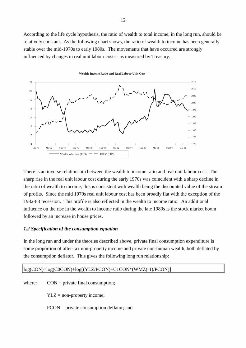
According to the life cycle hypothesis, the ratio of wealth to total income, in the long run, should be
relatively constant. As the following chart shows, the ratio of wealth to income has been generally
stable over the mid-1970s to early 1980s. The movements that have occurred are strongly
influenced by changes in real unit labour costs - as measured by Treasury.
Wealth-Income Ratio and Real Labour Unit Cost
14
15
16
17
18
19
20
21
Mar-70 Mar-72 Mar-74 Mar-76 Mar-78 Mar-80 Mar-82 Mar-84 Mar-86 Mar-88 Mar-90 Mar-92
1.70
1.75
1.80
1.85
1.90
1.95
2.00
2.05
2.10
2.15
Wealth to Income (RHS) RULC (LHS)
There is an inverse relationship between the wealth to income ratio and real unit labour cost. The
sharp rise in the real unit labour cost during the early 1970s was coincident with a sharp decline in
the ratio of wealth to income; this is consistent with wealth being the discounted value of the stream
of profits. Since the mid 1970s real unit labour cost has been broadly flat with the exception of the
1982-83 recession. This profile is also reflected in the wealth to income ratio. An additional
influence on the rise in the wealth to income ratio during the late 1980s is the stock market boom
followed by an increase in house prices.
1.2 Specification of the consumption equation
In the long run and under the theories described above, private final consumption expenditure is
some proportion of after-tax non-property income and private non-human wealth, both deflated by
the consumption deflator. This gives the following long run relationship:
log(CON)=log(C0CON)+log[(YLZ/PCON)+C1CON*(WMZ(-1)/PCON)]
where: CON = private final consumption;
YLZ = non-property income;
PCON = private consumption deflator; and
13
WMZ private sector non-human wealth.
The inclusion of the market value of private sector wealth in the TYRM model provides a channel
through which the financial and property markets can influence consumption behaviour of
households by affecting the value of financial and property assets. If asset prices were to rise faster
than consumption prices, for example, the market value of real wealth would increase, contributing
to an increase in consumption.
The above long run relationship can be interpreted as being consistent with either permanent income
or life-cycle hypotheses. Under a permanent income hypothesis, the coefficient C1CON could be
thought of as the average expected rate of return from non-human wealth. Therefore, the product of
the rate of return from non-human wealth and the stock of non-human wealth provides a flow of
property income to households. Alternatively, under a life-cycle hypothesis, C1CON could be
thought of as the average marginal propensity to consume out of non-human wealth and depends on
life-cycle factors such as age composition.
This long run relationship has two important properties. First, the long run marginal propensities to
consume out of non-property income are the same irrespective of the source. Second, in the long
run the marginal and average propensities to consume out of real labour income are equal.
In the short run, households appear to adjust their actual consumption only sluggishly toward their
long run levels. This common observation can be explained on the basis of habits, a general
tendency by households to smooth consumption, and uncertainty about whether changes are
persistent. Accordingly, private consumption is modelled using a first order partial adjustment
specification. Through the year changes in the unemployment rate (RNU) are also included and,
apart from representing a purely cyclical influence, may capture the additional effects of consumer
confidence and the distributional effects of changes in employment status (eg. individuals at the
margin of the workforce might have higher than average marginal propensities to consume).
Therefore the estimating equation was specified as:
log(CON) =(1-A0CON)*log(CON(-1))
+A0CON*{log(C0CON)+log[(YLZ/PCON)+C1CON*(WMZ(-1)/PCON)]}
+A2CON*[RNU-RNU(-4)]
This preferred specification was arrived at after some experimentation with other variables and
functional forms. Competing variables not included in the consumption function were changes in
non-property income, interest rates, and inflation. The change in non-property income was
statistically insignificant over the sample period suggesting that households are not liquidity
14
constrained; this result is consistent with the Blundell-Wignall, Browne, Cavaglia and Tarditi
(1992) study.
In theory, the interest rate should influence households' consumption decisions because it represents
the price of intertemporal substitution. However, the inclusion of interest rates and the yield curve
were unsuccessful given our framework discussed above. This result is consistent with other
studies (Hall 1988 and Mankiw 1989).
The inflation rate did have significant and negative effects on consumption over some estimation
periods, but not others. This was largely due to a correlation between the surge in inflation in the
mid 1970s and a weakening in consumption. Whether this consumption outcome was the result of
higher inflation or some other influence, such as uncertainty, is not clear. Further, any
mismeasurement of consumption prices will lead to a higher measure of the quantity of
consumption and this influence could be producing a negative correlation in the 1970s. Finally, the
influence of inflation over the 1980s was found to be statistically insignificant.
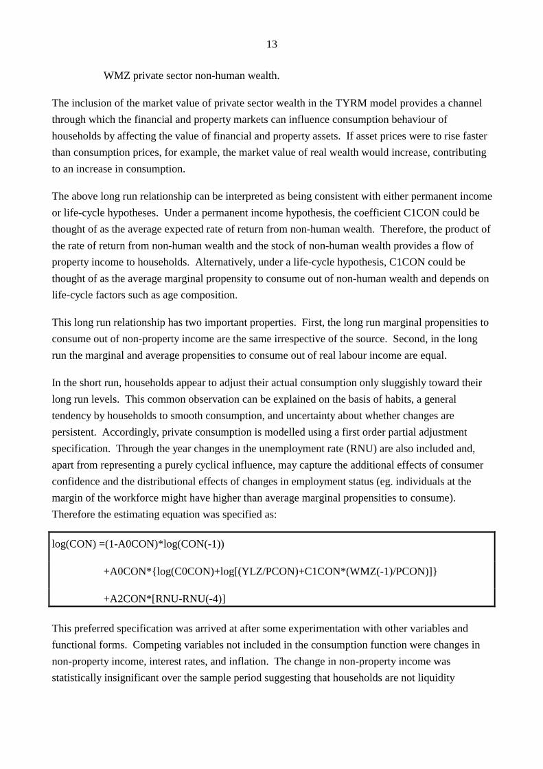
1.3 Estimation and interpretation of results
The consumption equation was estimated from the first quarter of 1980 to the fourth quarter of
1992. The choice of this period was based on two considerations: the lower quality of the wealth
data in the 1970s and the structural change in the availability and access to consumer credit in the
1980s. All coefficients of the estimated equation have significant and anticipated signs. The
following chart compares actual outcomes with a dynamic simulation of private final consumption
spending.
DYNAMIC SIMULATION OF TOTAL PRIVATE CONSUMPTION
log
leve
ls
10.20
10.30
10.40
10.50
10.60
10.70
10.80
10.90
11.00
Ma
r-7
0
Ma
r-7
1
Ma
r-7
2
Ma
r-7
3
Ma
r-7
4
Ma
r-7
5
Ma
r-7
6
Ma
r-7
7
Ma
r-7
8
Ma
r-7
9
Ma
r-8
0
Ma
r-8
1
Ma
r-8
2
Ma
r-8
3
Ma
r-8
4
Ma
r-8
5
Ma
r-8
6
Ma
r-8
7
Ma
r-8
8
Ma
r-8
9
Ma
r-9
0
Ma
r-9
1
Ma
r-9
2
Actual Simulated

15
As indicated, that the estimated equation fits the data reasonably well.
sample 1980:1 to 1992:4
Parameter Estimate t-Statistic
AOCON 0.2085 3.705
A2CON -0.0020 -2.736
C0CON 0.8118 15.963
C1CON 0.0132 3.804
The main features of the estimated equation are as follows. The coefficient C1CON was estimated
to be 0.0132. This can be interpreted as implying that the real rate of return of net income available
for consumption or savings from wealth is about 5 per cent per annum. It also implies that net
property income should be about 10 to15 per cent of total income, because private wealth is about 4
to 5 times the size of other income on an annual basis. This is consistent with the share of net
property incomes measured in the national accounts.
The coefficient C0CON was estimated to be 0.81, implying a saving ratio of about 20 per cent4 on
this basis. When private wealth is 4 to 5 times annual labour income the savings ratio is sufficient
to make private wealth grow at about 5 to 6 per cent per annum. Over the estimated period it
actually grew at 5 per cent, which is broadly consistent with this estimate.
The coefficient A0CON was estimated to be 0.2, implying that consumption adjusts to its long run
level with a mean lag of about 1 1/4 years.
The coefficient A2CON was estimated to be -0.002, implying that a one per cent increase in the
unemployment rate in a year would cause consumption to fall by 0.2 per cent. This result could be
due to increases in the level of uncertainty as the unemployment rate rises, causing households to
lift their savings.
2.0 DWELLING SECTOR
Aggregate dwelling investment is a small but cyclically volatile component of GDP, making it a
more important sector of the aggregate economy than its size would suggest. Further, dwelling
4. This savings ratio is not directly comparable to the ABS savings measure.

16
investment is one of the most interest sensitive components of GNE and so plays an important role
in the monetary policy transmission mechanism. In addition, the purchase of a dwelling represents
the largest single investment decision undertaken by most households. Private sector non-human
wealth data suggest that dwellings is about fifty six per cent of total private sector wealth thus
representing the largest component of wealth. Therefore, fluctuations in the price of dwellings have
a large impact on wealth. Movements in rents are important because it is one of the main
determinants house prices. Therefore, accurate modelling of dwelling investment is more important
to overall model properties than its size would suggest.
Our intention has been to model the dwelling sector in the current deregulated environment. This
means that data prior to 1986, when the housing market was regulated, was excluded from the
estimation period. This leaves a relatively small amount of data from which to test hypotheses,
resulting in more weight being placed on theoretical considerations when specifying equations in
this sector. This approach is different from that followed in NIF88 where the specification was
based on the market prior to deregulation.
In broad terms, dwelling investment is influenced by two major factors; the rate of return from
housing and the cost of funds. A primary determinant of the former is the rent price while the
interest rate is a major component of the latter. The dwelling sector in the TRYM model is analysed
by using two equations. The first is a consumer demand equation that determines the price of rents
and therefore the rate of return on dwellings. The second equation determines dwelling investment
using the factors mentioned above combined into a Tobin's Q-ratio.
2.1 Data considerations
Dwellings are demanded because they provide a flow of services over their lifetime. This flow will
be referred to here as rental services or rents. Data are collected by the ABS on average rents paid
in the market for rental accommodation. The average level of rents is then multiplied by the
number of dwellings to produce an estimate of the aggregate value of the consumption of rental
services. Owner-occupiers, like other owners of dwellings, are treated as other landlords and
tenants. They receive and pay rents (from themselves), pay expenses, and enjoy a rate of return on
their ownership of dwellings.
As noted above, these equations are only estimated from the first quarter of 1986. Financial
deregulation has integrated the market for housing loans with capital markets creating the potential
for large changes in the cyclical relationship between interest rates and dwelling investment. For
example, under a regulated lending environment the quantity of funds available for lending is
constrained and this, rather than the cost of funds, determines the level of transactions. In principal,
our approach to modelling dwelling investment could still be used in the regulated system if the cost

17
of the marginal dollar borrowed could be measured properly. Unfortunately, these data are not
available, thus limiting the estimation period to that mentioned above.
During the 1970s, there were large differences between the movements in the rent price series
collected by the ABS (in constructing the CPI) and the census data on average rents. This suggests
that either one or both of the series were incorrect in the 1970s and therefore the data for this period
are unsuitable for estimation. While this difference had fallen considerably by the 1980s, the
correlation between the relative price of rents (PCRE/PCNR) and relative expenditure share on rents
(CNR/CRE) appears to change around 1986. It is not clear why this is so. It may be a feature of the
data construction; for example, the data was spliced in 1984-85. Alternatively, the impact of a
regulated capital market may have affected this relationship. For example, the requirement of a
relatively high deposit by financial institutions may have forced many households into the rental
market. For these reasons it was decided to restrict the estimation period to commence in 1986.
2.2 Specification of the demand for rental services
The price of rent is determined by a simple consumer demand system consisting of rent and non-
rent expenditures. Consumers regard rental services as an (imperfect) substitute for other
consumption goods. This is captured by a constant elasticity of substitution (CES) utility function,
which is defined over the consumption of rental services and other consumption goods. Once
consumers have chosen the aggregate level of consumption spending based on their income and
wealth, they then choose the utility maximising proportion of rent consumption. The solution to
this maximisation problem yields the following demand curve.
log(CRE/CNR)=C0PCR-CDWSIG*log(PCRE*PCNR)
where: CRE=rent consumption;
CNR=other consumption goods;
CDWSIG=the elasticity of substitution between rental and non-rent consumption;
PCRE=the price of rents; and
PCNR=the price of non-rent consumption.
Because net investment is typically a small fraction of the capital stock, the stock of dwellings and
therefore the supply of rental services is essentially predetermined in the short run. Thus the
relative price of rents adjusts to ensure that demand equals the fixed level of supply. This suggests
that the demand equation should be inverted. The resulting equation determines the relative price of

18
rents as a function of the predetermined share of rental services. This yields an equation for the
equilibrium price of rents of the form:
log(PCRE/PCNR)=C0PCR-1/CDWSIG*log(CRE/CNR)
The demand and supply relation in the dwelling sector is depicted in the following chart.
pp' p
p'
S
D D'
S S'
D
Flow of rental services Flow of rental services
Panel (2)Panel (1)
ab
c a bc
In the short run, the supply of dwelling services - defined as the ratio of dwelling investment to
dwelling stock, is fixed. Therefore changes in demand for dwelling rents affect the price of rents in
the short run as indicated by the above equation. To illustrate the comparative static effects of the
dwelling market, suppose that our initial position is at point a in panel (1). Suppose also that private
final consumption rises because of an increase in income or wealth. This will cause the demand for
rental services to shift to the right from D to D'. If this increase in demand is not matched by an
equivalent rise in supply then, at unchanged rent prices, there will be an excess demand for dwelling
services - measured by the distance between points a and b. This will cause the price of rents to rise
(from p to p') until the new equilibrium is reached - which is at point c. Alternatively, if the supply
of rental services rises by more than private consumption - see panel (2), at unchanged rent prices
there will then be an excess supply for dwelling services - measured by the distance between points
a and b. This will cause the price of rents to fall (from p to p') until a new equilibrium is reached,
which is at point c.
The dynamic specification of the above model is as follows. Because most rents are fixed by
contracts for periods of a year or so, actual rents are likely to lag behind equilibrium rents as defined

19
by the above equation. Accordingly, an error correction specification was used for the rent price
equation.
∆log(PCRE/PCNR)=A2PCR*∆log(CNR/CRE)
-A0PCR*[log(PCRE(-1)/PCNR(-1)) - C0PCR
-1/CDWSIG*log(CNR(-1)/CRE(-1))]
2.3 Estimation and interpretation of results
The estimation results appear to be satisfactory given the difficulties with the data. The following
chart shows the actual and dynamic simulation of the relative price of rents to the price of non-rent
consumption.
DYNAMIC SIMULATION OF THE PRICE OF RENTS RELATIVE TO THE PRICE OF NON-RENT CONSUMPTION
per
cent
cha
nge
-0.070
-0.060
-0.050
-0.040
-0.030
-0.020
-0.010
0.000
0.010
Ma
r-8
6
Se
p-8
6
Ma
r-8
7
Se
p-8
7
Ma
r-8
8
Se
p-8
8
Ma
r-8
9
Se
p-8
9
Ma
r-9
0
Se
p-9
0
Ma
r-9
1
Se
p-9
1
Ma
r-9
2
Se
p-9
2
Actual Simulated
The estimated equation appears to fit the data reasonably well.
Sample 1986:1 to 1992:4
Parameter Estimate t-statistic
A0PCR 0.1113 2.736
A2PCR 0.4392 4.239
C0PCR -1.7002 -1.500

20
CDWSIG 0.8857 1.489
Any gap between the actual and desired equilibrium price of rents is closed by about 11 per cent per
quarter, implying a mean lag of adjustment of about 2 1/2 years.
The equation also implies that the elasticity of substitution between rents and non-rent consumption
is 0.88. This estimate is not well determined but is at a sensible level and consistent with other
studies. For example, Yates (1981) reports some cross section estimates of this elasticity using two
different data sets. For one data set, her estimates ranged from 0.701 to 0.871. Estimates using the
other data set ranged from 0.874 to 1.256. These elasticities are similar to those found in overseas
studies (Yates, 1981, page 321). The TRYM estimate of 0.89 is within the range of these estimates
and below the value of unity imposed in the AEM model. Other feature of the above equation is
that an increase of one per cent in non-rent consumption, among other things, increases the relative
price of rents by 0.43 per cent after one quarter.
2.4 Specification of the supply of rental services (dwelling investment)
Dwelling investment is specified using a comparison of the rate of return to the cost of funds. This
is equivalent to a comparison of the market and replacement values of dwelling, in the spirit of a
Tobin Q-ratio. The Q-ratio for dwellings (QRATH), defined as the ratio of the equilibrium rate of
return on the dwelling stock to the cost of funds, is the primary determinant of dwelling investment.
The ratio has the following interpretation. When the Q-ratio is equal to one, dwelling investment
will be sufficient to yield the desired level of growth of the dwellings stock (KDW). When the Q-
ratio is greater than one, households invest more in dwellings and when the Q-ratio is less than one
households will tend to invest less.
The equilibrium rate of return on dwellings (ER) is calculated as the ratio of the price of rents
(PCRE) to the implicit price deflator for dwelling investment (PIDW), adjusted for the rate of tax on
the consumption of rents (RTCRE) and the amount of rental services produced each quarter by a
unit of dwelling capital.
ER=(1-RTCRE)*PCRE*(0.035306)/PIDW;
The constant 0.035306 is the historical average ratio of production of dwelling rents to the dwelling
capital.
In the long run, the cost of funds for dwellings will be equal to the 10 year bond rate (RGL). In the
short run, however, the cost of funds for dwelling investment may also be influenced by short term
interest rates. We let the data determine the relative importance of long and short term interest
rates. In particular, the actual cost of funds for investment in dwellings is calculated as a weighted
21
average of long bond rates (RGL) and the 90 day bank bill rate (R90), less long run inflationary
expectations and the depreciation rate on dwellings (RDKDW). The method used to measure
INFEXP (inflationary expectations) is discussed in the Financial Sector.
Cost of funds=((C1DW*RGL+(1-C1DW)*R90)-INFEXP/400)*RDKDW
QRATH is therefore defined as follows:
QRATH=[(1-RTCRE)*PCRE*(0.035306)/PIDW]/
[((C1DW*RGL+(1-C1DW)*R90)-INFEXP/400)*RDKDW]
In the long run, when the Q-ratio is at unity, investment in dwellings (IDW) - as a ratio of the
dwelling capital stock (KDW) - is at a level sufficient to ensure that dwelling capital grows at the
equilibrium growth rate of the economy (GR) adjusted for the rate of depreciation on the capital
stock (RDKDW). GR is the sum of the growth of underlying efficiency (and therefore per capita)
growth in the economy and growth in the adult population.
The lags between a change in the Q-ratio and dwelling investment is of particular interest here.
Both contemporaneous and lagged values of the Q-ratio are found to impact on investment in
dwellings. This is consistent with the influence of lags in households' response to changes in
economic fundamentals due, for example, to the time taken in planning housing investment and in
gaining approval to start construction. Due to the relatively small sample size and the presence of
serial correlation among the Q-ratios, the size and significance of the coefficients on the different
lagged values of the Q-ratio tended to vary in an erratic and implausible fashion. The estimated
parameters on different lags of the Q-ratio have been constrained to be the same. This smooths the
reaction of dwelling investment to the Q-ratio and gives a significant overall coefficient. This
constraint is accepted by the data.
Past dwelling investment is also used to explain contemporaneous dwelling investment. This
captures the discrete nature of dwelling investment that may take longer than a quarter to complete
and the associated inertia or serial correlation in dwelling investment behaviour.
To capture some of the short term influences on dwelling investment, labour market pressures, such
as the unemployment rate, are included. In particular, if the actual unemployment rate (RNU) is
higher than the equilibrium rate (NAIRU), households' confidence will fall and this will lead to a
reduction in investment in dwellings. The data appear to accept this confidence, or uncertainty
effect on dwelling investment. The preferred dwelling investment equation is therefore as follows:

22
IDW/KDW(-1)= [exp(GR)-1+RDKDW]*(1-A1DW-A2DW-A3DW-A4DW)
+A1DW*[IDW(-1)/KDW(-2)]+A2DW*[IDW(-2)/KDW(-3)]
+A3DW*[IDW(-3)/KDW(-4)]+A4DW*[IDW(-4)/KDW(-5)]
+A0DW*QRATH+A0DW*QRATH(-1)+A0DW*QRATH(-2)
+A0DW*QRATH(-3)+A0DW*QRATH(-4)
+A5DW*[RNU-NAIRU]
2.5 Estimation and interpretations of results
The following chart shows the actual and dynamic simulation of the ratio of dwelling investment to
dwelling stock.
DYNAMIC SIMULATION OF THE RATIO OF DWELLING INVESTMENT TO DWELLINGSTOCK
ratio
of d
wel
ling
inve
stm
ent t
o dw
ellin
g st
ock
0.008
0.009
0.009
0.010
0.010
0.011
0.011
0.012
0.012
0.013
Ma
r-8
6
Se
p-8
6
Ma
r-8
7
Se
p-8
7
Ma
r-8
8
Se
p-8
8
Ma
r-8
9
Se
p-8
9
Ma
r-9
0
Se
p-9
0
Ma
r-9
1
Se
p-9
1
Ma
r-9
2
Se
p-9
2
Actual Simulated
As indicated, the estimated equation tends to consistently underestimate extent of the dwellings
cycle. There are probably additional cyclical effects due to expectations of capital gains or the
availability of funds not incorporated in the above specification. Given the small sample size, we
have avoided the temptation to overfit the data using variables that the future may show were only
important over the past cycle.
Sample: 1986:1 to 1992:4
Parameter Estimate t-statistic

23
A0DW 0.000339 3.28
A1DW 0.417 2.386
A2DW 0.521 3.171
A3DW -0.0314 -0.216
A4DW -0.256 -2.111
A5DW -0.0000959 -2.408
C1DW 0.351 3.043
The equation implies that if the rate of return from investing in dwellings is 10 per cent greater than
the cost of obtaining funding for the investment, dwelling investment as a ratio of the capital stock
will increase by 0.017 per cent after 5 quarters.
The equation also implies that:
• an increase in investment in dwellings today will be followed by higher investment for two
quarters and then two quarters when the quantity of dwelling investment falls as a proportion
of the capital stock. This lag structure seems to plausibly reflect the nature of investment in
housing;
• if the actual unemployment rate exceeds the NAIRU by 1 per cent, dwelling investment will
fall by about [0.0001] as a percentage of the capital stock; and
• the estimate for C1DW implies that about 2/3 of the weight should go on long term interest
rates and about 1/3 on short rates when measuring the cost of funds in the Q-ratio.
3.0 LABOUR SUPPLY BEHAVIOUR
The notion of labour supply encompasses several important dimensions that include the size and
demographic composition of the population, the proportion of the working-age population that is
employed or seeking employment (ie. the participation rate), the number of hours worked per period
(ie. per week, per month or per year) and the quality of labour (ie health, nutrition and education).
However, econometric studies of labour supply have traditionally focused on a smaller subset of
factors, namely decisions on whether to participate in the labour force and on the number of hours
to work. This approach is also adopted in the TRYM model.

24
Studies of labour supply suggest that a range of factors influence an individual's decision to
participate in the labour force. These include: age, gender, level of real wages and labour market
opportunities. There are other variables that are difficult to include in macroeconometric models
such as: attitudes towards work-leisure, household structures and fixed costs associated with work
(eg the availability for child-care facilities, loss of government benefits upon employment, travel
and other work related expenses).
At the aggregate level, the conventional approach to modelling labour supply is to ignore the issue
of aggregation by assuming a homogeneous labour market. In reality, labour markets are segmented
with different wages and hours of work being offered across different labour markets. Because
macro models do not explicitly take account of the segmentation of labour markets, their ability to
explain important compositional changes in the labour force - such as shifts towards part-time work
- is limited.
There are important issues at both the aggregate and disaggregate levels. At the disaggregate level,
the most important considerations appear to be age and gender and by type of employment. There
also appears to be differences in employment elasticities between primary and secondary workers.
At the aggregate level, many of these issues are relatively less important because the age and gender
composition of the population change little and slowly. The most important issues are the effects of
higher incomes and on participation rates. Since the focus in the TRYM model is to explain
aggregate behaviour, we will be examining the average responses across divergent groups.
Further because labour supply equation in the TRYM model is estimated on an hours basis, we are
able to broadly account for the shift towards part-time employment.
3.1 Data considerations
Over the 1980s and early 1990s, the labour force grew at an average rate of [2.5 ] per cent per year,
although there are large variations in the annual growth rates. The significant variations in the
annual growth rates reflect both varying adult population growth rates and demographic changes.
There have also been significant compositional changes in the labour force participation rates
measured by gender and type of work sought (and found).

25
LABOUR FORCE PARTICIPATION RATE BY GENDER
60
62
64
66
68
70
72
74
76
78
80
Fe
b-7
8
Fe
b-7
9
Fe
b-8
0
Fe
b-8
1
Fe
b-8
2
Fe
b-8
3
Fe
b-8
4
Fe
b-8
5
Fe
b-8
6
Fe
b-8
7
Fe
b-8
8
Fe
b-8
9
Fe
b-9
0
Fe
b-9
1
Fe
b-9
2
Fe
b-9
3
40
42
44
46
48
50
52
54
56
58
60
MALES (RHS) FEMALES (LHS)
Full-time participation rates among males of all ages have shown a trend decline while for females
there has been an upward trend. This upward trend for females is particularly significant for part-
time participation rates (Fahrer and Heath 1992). These trends have also been evident in the United
States (Smith and Ward 1985) and other similar countries. Therefore, gender accounts for
substantial variation in participation rates between individuals.
The upward trend of female participation rates reflects a number of factors. Rising male real wages,
and therefore real incomes, would suggest that married woman should have reduced their
commitment to the labour force (ie the income effect), but this effect has been more than offset by
increases in female wage rates, availability of child care facilities and employment possibilities that
are available to women (ie substitution effect). Further, improved educational achievements by
females not only have increased real wages but have also resulted in changed attitudes towards
obtaining meaningful employment outside their homes. Other factors include the increased
availability of household appliances (which are labour-saving), have encouraged females to seek full
and part-time employment.
The overall trend decline in male participation rates has been attributed largely to the decline in full-
time employment. However, there are significant changes within this aggregate result.
Disaggregated data suggest that the fall in participation rates is greatest among older ages, possibly
suggesting early retirements, but there have been strong increases in part-time participation rates
among 15-24 year old males, perhaps reflecting increased participation in full-time education
(DEET 1991).
These trends in the labour force suggest that labour supply should explicitly take account of at least
the full-time and part-time status of labour supply and the average hours worked per person.
26
However, the traditional approach to the modelling of labour supply has been on a heads basis. This
is reflected in the NIF10, NIF88, AMPS and AEM models. This approach to labour supply assumes
that individuals do not respond to the hours of work available when deciding whether to participate
in the work force. Such decisions are particularly relevant to individuals who operate on a
households basis. For example, reduced working hours by one adult may allow another adult to
increase their participation in the labour force. Alternatively, reduced working hours by one adult
may reduce household incomes and induce other adults to seek paid employment.
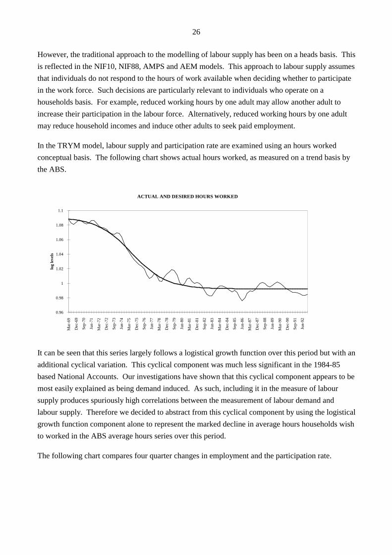
In the TRYM model, labour supply and participation rate are examined using an hours worked
conceptual basis. The following chart shows actual hours worked, as measured on a trend basis by
the ABS.
ACTUAL AND DESIRED HOURS WORKED
log
leve
ls
0.96
0.98
1
1.02
1.04
1.06
1.08
1.1
Ma
r-6
9
De
c-6
9
Se
p-7
0
Jun
-71
Ma
r-7
2
De
c-7
2
Se
p-7
3
Jun
-74
Ma
r-7
5
De
c-7
5
Se
p-7
6
Jun
-77
Ma
r-7
8
De
c-7
8
Se
p-7
9
Jun
-80
Ma
r-8
1
De
c-8
1
Se
p-8
2
Jun
-83
Ma
r-8
4
De
c-8
4
Se
p-8
5
Jun
-86
Ma
r-8
7
De
c-8
7
Se
p-8
8
Jun
-89
Ma
r-9
0
De
c-9
0
Se
p-9
1
Jun
-92
It can be seen that this series largely follows a logistical growth function over this period but with an
additional cyclical variation. This cyclical component was much less significant in the 1984-85
based National Accounts. Our investigations have shown that this cyclical component appears to be
most easily explained as being demand induced. As such, including it in the measure of labour
supply produces spuriously high correlations between the measurement of labour demand and
labour supply. Therefore we decided to abstract from this cyclical component by using the logistical
growth function component alone to represent the marked decline in average hours households wish
to worked in the ABS average hours series over this period.
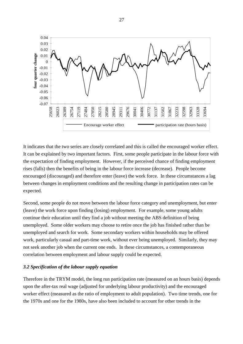
The following chart compares four quarter changes in employment and the participation rate.
27
four
qua
rter
cha
nge
-0.07
-0.06
-0.05
-0.04
-0.03
-0.02
-0.01
0
0.01
0.02
0.03
0.04
25
65
8
26
02
3
26
38
9
26
75
4
27
11
9
27
48
4
27
85
0
28
21
5
28
58
0
28
94
5
29
31
1
29
67
6
30
04
1
30
40
6
30
77
2
31
13
7
31
50
2
31
86
7
32
23
3
32
59
8
32
96
3
33
32
8
33
69
4
Encourage worker effect participation rate (hours basis)
It indicates that the two series are closely correlated and this is called the encouraged worker effect.
It can be explained by two important factors. First, some people participate in the labour force with
the expectation of finding employment. However, if the perceived chance of finding employment
rises (falls) then the benefits of being in the labour force increase (decrease). People become
encouraged (discouraged) and therefore enter (leave) the work force. In these circumstances a lag
between changes in employment conditions and the resulting change in participation rates can be
expected.
Second, some people do not move between the labour force category and unemployment, but enter
(leave) the work force upon finding (losing) employment. For example, some young adults
continue their education until they find a job without meeting the ABS definition of being
unemployed. Some older workers may choose to retire once the job has finished rather than be
unemployed and search for work. Some secondary workers within households may be offered
work, particularly casual and part-time work, without ever being unemployed. Similarly, they may
not seek another job when the current one ends. In these circumstances, a contemporaneous
correlation between employment and labour supply could be expected.
3.2 Specification of the labour supply equation
Therefore in the TRYM model, the long run participation rate (measured on an hours basis) depends
upon the after-tax real wage (adjusted for underlying labour productivity) and the encouraged
worker effect (measured as the ratio of employment to adult population). Two time trends, one for
the 1970s and one for the 1980s, have also been included to account for other trends in the

28
participation rates- due to demographic factors, and structural changes in the work force that
occurred over the 1980s. This gives the following equilibrium relationship for the participation rate.
log(NLF*NHLR/NAP)=C1LS+C2LS*log[NT*NHLR/NAP]
+C3LS*[log((1-RTN)*WT/(NH*PCON))-CLAM*QTIME]
+C4LS*D80*(QTIME+10.725)
+C5LS*QTIME
In the short run, movements in the participation rate are also explained by an additional term that
captures changes in the encouraged worker effect in the current quarter. An error correction
specification was used to incorporate the long and short run responses.
∆ log [(NLF*NHLR)/NAP] =A1LS*∆log (NT/NAP)
-A2LS*∆log(NT(-2)/NAP(-2))
-A3LS*{log[NLF(-1)*NHLR(-1)/NAP(-1)]
+C1LS-C2LS*log[NT(-1)*NHLR(-1)/NAP(-1)
-C3LS*[log((1-RTN(-1))*WT(-1)/(NH(-1)*PCON(-1))
-CLAM*QTIME(-1)]
-C4LS*D80(-1)*(QTIMF(-1)+10.725)-C5LS*QTIMF(-1)}
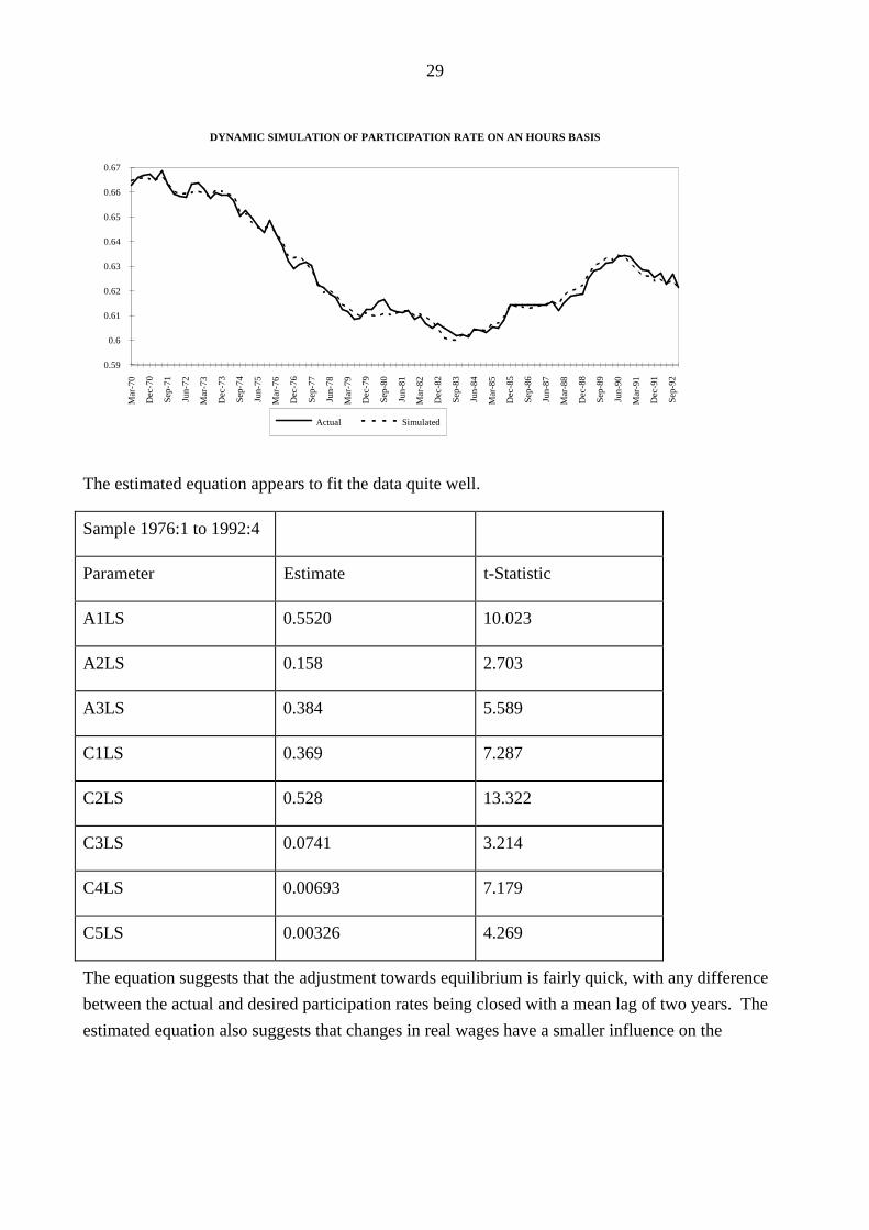
3.3 Estimation and interpretations of results
The labour supply equation was estimated from the first quarter of 1976 to the fourth quarter of
1992. All estimates have anticipated signed and significant. The following chart shows the actual
and dynamic simulation of the participation rate.
29
DYNAMIC SIMULATION OF PARTICIPATION RATE ON AN HOURS BASIS
0.59
0.6
0.61
0.62
0.63
0.64
0.65
0.66
0.67
Ma
r-7
0
De
c-7
0
Se
p-7
1
Jun
-72
Ma
r-7
3
De
c-7
3
Se
p-7
4
Jun
-75
Ma
r-7
6
De
c-7
6
Se
p-7
7
Jun
-78
Ma
r-7
9
De
c-7
9
Se
p-8
0
Jun
-81
Ma
r-8
2
De
c-8
2
Se
p-8
3
Jun
-84
Ma
r-8
5
De
c-8
5
Se
p-8
6
Jun
-87
Ma
r-8
8
De
c-8
8
Se
p-8
9
Jun
-90
Ma
r-9
1
De
c-9
1
Se
p-9
2
Actual Simulated
The estimated equation appears to fit the data quite well.
Sample 1976:1 to 1992:4
Parameter Estimate t-Statistic
A1LS 0.5520 10.023
A2LS 0.158 2.703
A3LS 0.384 5.589
C1LS 0.369 7.287
C2LS 0.528 13.322
C3LS 0.0741 3.214
C4LS 0.00693 7.179
C5LS 0.00326 4.269
The equation suggests that the adjustment towards equilibrium is fairly quick, with any difference
between the actual and desired participation rates being closed with a mean lag of two years. The
estimated equation also suggests that changes in real wages have a smaller influence on the

30
participation rate than the encouraged worker effect5. The elasticity with respect to wages was
estimated to be 0.07 per cent compared to the elasticity with respect to encourage worker effect of
0.53 per cent. Other interesting results are the coefficient on the time trends. They suggest that the
participation rate grew on average by 0.33 per cent per quarter more during the 1970s than may have
been expected given the employment ratio and real after-tax wages, while during the 1980s the
participation rate grew by an average of 0.69 per cent per quarter faster.
4.0 CONCLUSION
This paper models households decisions regarding consumption/saving, work/leisure and dwelling
investment in a simple and transparent way. The approach adopted here incorporates both
theoretical and data considerations.
All equations are specified and estimated using the recently rebased National Accounts data. We
have been careful to allow the data to validate linkages between sectors where inter linkages appear
possible. Developments in the labour market, such as the level and changes in employment and
unemployment for example, affect consumption, dwelling investment and labour supply decisions.
These linkages are consistent with theoretical considerations.
Consumption is based on an Ando-Modigliani specification, though it could also be interpreted in a
manner consistent with a permanent income hypothesis. The estimate parameters are significant
and have sensible economic interpretations. One key finding is that the short run marginal
propensity to consume out of wages and government transfers is very low once our measure of
wealth is included in the specification.
Our modelling of the dwelling sector is confined to the period of deregulation. This constraint on
Australia's experience with a deregulated financial market means that the data is limited to only one
complete cycle. Nevertheless, a sensible specification was chosen and estimated yielding plausible
results. The specification includes a Q-ratio that captures interest rates and consumption levels
through rent prices, and a variable to reflect the state of the labour market. As more data becomes
available we will be able to test our specification more rigorously.
Finally, our equation for labour supply captures the important employment, income and average
hours worked linkages that are important to a macro economist. All the estimated coefficients are
significant and have sensible macroeconomic interpretations. The modelling of aggregate labour
5. This result is consistent with other studies that show changes in real wages do not have a strong affect labour supply.An important reason for this relatively weak response to changes in real wages is due to the differing reaction of workersin different wage categories- ie high vs low paid workers.

31
supply in TRYM will never be as complete as more detailed but partial studies because it only
explains participation rates in terms of endogenous macroeconomic variables and time trends.
Nevertheless, TRYM's labour supply equation captures the broad features of the data quite well.
32
References
Ando, A and Modigliani, F (1963), "The Life-Cycle Hypothesis of Saving: Aggregate Implications
and Tests", American Economic Review, vol. 53, pages 55-84.
Barro, Robert J (1974), "Are Government Bonds Net Wealth?", Journal of Political Economy, vol.
82, pages 1095-1117.
Blander, Alan S, and Deaton, Angus (1985), "The Time Series Consumption Function Revisited",
Brookings Papers on Economic Activity, 2, pages 465-521.
Blundell-Wignall, A, Browne, F, Cavaglia, S and Tarditi, A (1992), " Financial Liberalisation and
Consumption Behaviour", Reserve Bank of Australia: Research Discussion Paper (RDP) 9209.
Callen, Tim (1991), "Estimates of Private Sector Wealth", Reserve Bank of Australia: Research
Discussion Paper.
Campbell, John Y and Mankiw, George N (1989), "Consumption, Income, and Interest Rates:
Reinterpreting the Time-Series Evidence", NBER Macroeconomics Annual, pages 185-26.
Delong, J and Summers, L (1986), "The Changing Cyclical Variability of Economic Activity in the
United States", in R J. Gordon ed., "The American Business Cycle: Continuity and Change",
Chicago University of Chicago Press.
Department of Employment, Education and Training (1991), "Australia's Workforce in the Year
2001", June, AGPS.
Fahrer, J and Heath, A (1992), "The Evolution of Employment and Unemployment in Australia",
Reserve Bank of Australia: Research Discussion Paper (RDP) 9215.
Friedman, Milton (1957), "A Theory of Consumption Function", Princeton, N.J.: Princeton
University Press.
Hall, Robert E (1988), "Intertemporal Substitution and Consumption", Journal of Political
Economy, 96, pages 339-357.
Hayashi, F (1985), "Tests For Liquidity Constraints: A Critical Survey", National Bureau of
Economic Research, Working Paper No: 1720.
Piggott, J (1987), "The Nation's Private Wealth - Some New Calculations for Australia", The
Economic Record, March, pages 61-79.

33
Smith, James P and Ward, M (1985), "Time Series Growth in the Female Labour Force", Journal of
Labour Economics, 3:1, January, Supplement, pages S59-S90.