A&A 594, A24 (2016)DOI: 10.1051/0004-6361/201525833c© ESO 2016

Astronomy&Astrophysics

Planck 2015 results Special feature

Planck 2015 results

XXIV. Cosmology from Sunyaev-Zeldovich cluster counts

Planck Collaboration: P. A. R. Ade97, N. Aghanim65, M. Arnaud81, M. Ashdown77, 6, J. Aumont65, C. Baccigalupi95, A. J. Banday108, 11,R. B. Barreiro72, J. G. Bartlett1, 74, N. Bartolo33, 73, E. Battaner110, 111, R. Battye75, K. Benabed66, 107, A. Benoît63, A. Benoit-Lévy27, 66, 107,

J.-P. Bernard108, 11, M. Bersanelli36, 53, P. Bielewicz90, 11, 95, J. J. Bock74, 13, A. Bonaldi75,?, L. Bonavera72, J. R. Bond10, J. Borrill16, 101,F. R. Bouchet66, 99, M. Bucher1, C. Burigana52, 34, 54, R. C. Butler52, E. Calabrese104, J.-F. Cardoso82, 1, 66, A. Catalano83, 80, A. Challinor69, 77, 14,

A. Chamballu81, 18, 65, R.-R. Chary62, H. C. Chiang30, 7, P. R. Christensen91, 39, S. Church103, D. L. Clements61, S. Colombi66, 107,L. P. L. Colombo26, 74, C. Combet83, B. Comis83, F. Couchot79, A. Coulais80, B. P. Crill74, 13, A. Curto72, 6, 77, F. Cuttaia52, L. Danese95,

R. D. Davies75, R. J. Davis75, P. de Bernardis35, A. de Rosa52, G. de Zotti49, 95, J. Delabrouille1, F.-X. Désert58, J. M. Diego72, K. Dolag109, 87,H. Dole65, 64, S. Donzelli53, O. Doré74, 13, M. Douspis65, A. Ducout66, 61, X. Dupac42, G. Efstathiou69, F. Elsner27, 66, 107, T. A. Enßlin87,

H. K. Eriksen70, E. Falgarone80, J. Fergusson14, F. Finelli52, 54, O. Forni108, 11, M. Frailis51, A. A. Fraisse30, E. Franceschi52, A. Frejsel91,S. Galeotta51, S. Galli76, K. Ganga1, M. Giard108, 11, Y. Giraud-Héraud1, E. Gjerløw70, J. González-Nuevo22, 72, K. M. Górski74, 112, S. Gratton77, 69,

A. Gregorio37, 51, 57, A. Gruppuso52, J. E. Gudmundsson105, 93, 30, F. K. Hansen70, D. Hanson88, 74, 10, D. L. Harrison69, 77, S. Henrot-Versillé79,C. Hernández-Monteagudo15, 87, D. Herranz72, S. R. Hildebrandt74, 13, E. Hivon66, 107, M. Hobson6, W. A. Holmes74, A. Hornstrup19, W. Hovest87,

K. M. Huffenberger28, G. Hurier65, A. H. Jaffe61, T. R. Jaffe108, 11, W. C. Jones30, M. Juvela29, E. Keihänen29, R. Keskitalo16, T. S. Kisner85,R. Kneissl41, 8, J. Knoche87, M. Kunz20, 65, 3, H. Kurki-Suonio29, 47, G. Lagache5, 65, A. Lähteenmäki2, 47, J.-M. Lamarre80, A. Lasenby6, 77,

M. Lattanzi34, C. R. Lawrence74, R. Leonardi9, J. Lesgourgues67, 106, F. Levrier80, M. Liguori33, 73, P. B. Lilje70, M. Linden-Vørnle19,M. López-Caniego42, 72, P. M. Lubin31, J. F. Macías-Pérez83, G. Maggio51, D. Maino36, 53, N. Mandolesi52, 34, A. Mangilli65, 79, M. Maris51,P. G. Martin10, E. Martínez-González72, S. Masi35, S. Matarrese33, 73, 44, P. McGehee62, P. R. Meinhold31, A. Melchiorri35, 55, J.-B. Melin18,

L. Mendes42, A. Mennella36, 53, M. Migliaccio69, 77, S. Mitra60, 74, M.-A. Miville-Deschênes65, 10, A. Moneti66, L. Montier108, 11, G. Morgante52,D. Mortlock61, A. Moss98, D. Munshi97, J. A. Murphy89, P. Naselsky92, 40, F. Nati30, P. Natoli34, 4, 52, C. B. Netterfield23, H. U. Nørgaard-Nielsen19,

F. Noviello75, D. Novikov86, I. Novikov91, 86, C. A. Oxborrow19, F. Paci95, L. Pagano35, 55, F. Pajot65, D. Paoletti52, 54, B. Partridge46, F. Pasian51,G. Patanchon1, T. J. Pearson13, 62, O. Perdereau79, L. Perotto83, F. Perrotta95, V. Pettorino45, F. Piacentini35, M. Piat1, E. Pierpaoli26,

D. Pietrobon74, S. Plaszczynski79, E. Pointecouteau108, 11, G. Polenta4, 50, L. Popa68, G. W. Pratt81, G. Prézeau13, 74, S. Prunet66, 107, J.-L. Puget65,J. P. Rachen24, 87, R. Rebolo71, 17, 21, M. Reinecke87, M. Remazeilles75, 65, 1, C. Renault83, A. Renzi38, 56, I. Ristorcelli108, 11, G. Rocha74, 13,

M. Roman1, ∗, C. Rosset1, M. Rossetti36, 53, G. Roudier1, 80, 74, J. A. Rubiño-Martín71, 21, B. Rusholme62, M. Sandri52, D. Santos83,M. Savelainen29, 47, G. Savini94, D. Scott25, M. D. Seiffert74, 13, E. P. S. Shellard14, L. D. Spencer97, V. Stolyarov6, 102, 78, R. Stompor1,

R. Sudiwala97, R. Sunyaev87, 100, D. Sutton69, 77, A.-S. Suur-Uski29, 47, J.-F. Sygnet66, J. A. Tauber43, L. Terenzi96, 52, L. Toffolatti22, 72, 52,M. Tomasi36, 53, M. Tristram79, M. Tucci20, J. Tuovinen12, M. Türler59, G. Umana48, L. Valenziano52, J. Valiviita29, 47, B. Van Tent84, P. Vielva72,

F. Villa52, L. A. Wade74, B. D. Wandelt66, 107, 32, I. K. Wehus74, 70, J. Weller109, S. D. M. White87, D. Yvon18, A. Zacchei51, and A. Zonca31

(Affiliations can be found after the references)

Received 6 February 2015 / Accepted 14 June 2016

ABSTRACT

We present cluster counts and corresponding cosmological constraints from the Planck full mission data set. Our catalogue consists of 439 clustersdetected via their Sunyaev-Zeldovich (SZ) signal down to a signal-to-noise ratio of 6, and is more than a factor of 2 larger than the 2013 Planckcluster cosmology sample. The counts are consistent with those from 2013 and yield compatible constraints under the same modelling assumptions.Taking advantage of the larger catalogue, we extend our analysis to the two-dimensional distribution in redshift and signal-to-noise. We usemass estimates from two recent studies of gravitational lensing of background galaxies by Planck clusters to provide priors on the hydrostaticbias parameter, (1 − b). In addition, we use lensing of cosmic microwave background (CMB) temperature fluctuations by Planck clusters asan independent constraint on this parameter. These various calibrations imply constraints on the present-day amplitude of matter fluctuations invarying degrees of tension with those from the Planck analysis of primary fluctuations in the CMB; for the lowest estimated values of (1 − b)the tension is mild, only a little over one standard deviation, while it remains substantial (3.7σ) for the largest estimated value. We also examineconstraints on extensions to the base flat ΛCDM model by combining the cluster and CMB constraints. The combination appears to favournon-minimal neutrino masses, but this possibility does little to relieve the overall tension because it simultaneously lowers the implied value ofthe Hubble parameter, thereby exacerbating the discrepancy with most current astrophysical estimates. Improving the precision of cluster masscalibrations from the current 10%-level to 1% would significantly strengthen these combined analyses and provide a stringent test of the baseΛCDM model.

Key words. cosmological parameters – large-scale structure of Universe

? Corresponding authors: A. Bonaldi, e-mail: anna.bonaldi@manchester.ac.uk;M. Roman, e-mail: matthieu.roman@apc.univ-paris7.fr

Article published by EDP Sciences A24, page 1 of 19

A&A 594, A24 (2016)

1. Introduction

Galaxy cluster counts are a standard cosmological tool thathas found powerful application in recent Sunyaev-Zeldovich(SZ) surveys performed by the Atacama Cosmology Tele-scope (ACT, Swetz et al. 2011; Hasselfield et al. 2013), theSouth Pole Telescope (SPT, Carlstrom et al. 2011; Benson et al.2013; Reichardt et al. 2013; Bocquet et al. 2015), and the Plancksatellite1 (Tauber et al. 2010; Planck Collaboration I 2011). Theabundance of clusters and its evolution are sensitive to the cos-mic matter density, Ωm, and the present amplitude of densityfluctuations, characterized by σ8, the rms linear overdensity inspheres of radius 8h−1 Mpc. The primary cosmic microwavebackground (CMB) anisotropies, on the other hand, reflect thedensity perturbation power spectrum at the time of recombina-tion. This difference is important because a comparison of theamplitude of the perturbations at the two epochs tests the evolu-tion of density perturbations from recombination until today, en-abling us to look for possible extensions to the base Λcold darkmatter (CDM) model, such as non-minimal neutrino masses ornon-zero curvature.

Launched on 14 May 2009, Planck scanned the entire skytwice a year from 12 August 2009 to 23 October 2013, at angu-lar resolutions from 33′ to 5′ with two instruments: the Low Fre-quency Instrument (LFI; Bersanelli et al. 2010; Mennella et al.2011), covering bands centred at 30, 44, and 70 GHz, andthe High Frequency Instrument (HFI; Lamarre et al. 2010;Planck HFI Core Team 2011), covering bands centred at 100,143, 217, 353, 545, and 857 GHz.

An initial set of cosmology results appeared in 2013, basedon the first 15.5 months of data (Planck Collaboration I 2014),including cosmological constraints from the redshift distribu-tion of 189 galaxy clusters detected at signal-to-noise (S/N)>7 (hereafter, our “first analysis” or the “2013 analysis”,Planck Collaboration XX 2014). The present paper is part of thesecond set of cosmology results obtained from the full missiondata set; it is based on an updated cluster sample introduced in anaccompanying paper (the PSZ2, Planck Collaboration I 2016).

Our first analysis found fewer clusters than predicted byPlanck’s base ΛCDM model, expressed as a tension betweenthe cluster constraints on (Ωm, σ8) and those from the primaryCMB anisotropies (Planck Collaboration XVI 2014). This couldreflect the need for an extension to the base ΛCDM model or in-dicate that clusters are more massive than determined by the SZsignal-mass scaling relation adopted in 2013.

The cluster mass scale is the largest source of uncertainty ininterpretation of the cluster counts. We based our first analysison X-ray mass proxies that rely on the assumption of hydrostaticequilibrium. Simulations demonstrate that this assumption canbe violated by bulk motions in the gas or by non-thermal sourcesof pressure (e.g., magnetic fields or cosmic rays, Nagai et al.2007; Piffaretti & Valdarnini 2008; Meneghetti et al. 2010). Sys-tematics in the X-ray analyses (e.g., instrument calibration, tem-perature structure in the gas) could also bias the mass measure-ments significantly (Rasia et al. 2006, 2012). We quantified ourignorance of the true mass scale of clusters with a mass bias pa-rameter that was varied over the range 0−30%, with a baselinevalue of 20% (see below for the definition of the mass bias),

1 Planck (http://www.esa.int/Planck) is a project of the Euro-pean Space Agency (ESA) with instruments provided by two scientificconsortia funded by ESA member states and led by Principal Investi-gators from France and Italy, telescope reflectors provided through acollaboration between ESA and a scientific consortium led and fundedby Denmark, and additional contributions from NASA (USA).

as suggested by numerical simulations (see the Appendix ofPlanck Collaboration XX 2014).

Gravitational lensing studies of the SZ signal-mass relationare particularly valuable in this context because they are in-dependent of the dynamical state of the cluster (Marrone et al.2012; Planck Collaboration Int. III 2013), although they also,of course, can be affected by systematic effects (e.g.,Becker & Kravtsov 2011). New, more precise lensing mass mea-surements for Planck clusters have appeared since our 2013analysis (von der Linden et al. 2014b; Hoekstra et al. 2015). Weincorporate these new results as prior constraints on the massbias in the present analysis. Two other improvements over 2013are the use of a larger cluster catalogue and analysis of the countsin signal-to-noise as well as redshift.

In addition, we apply a novel method to measure clustermasses through lensing of the CMB anisotropies. This method,presented in Melin & Bartlett (2015), enables us to use Planckdata alone to constrain the cluster mass scale. It provides an im-portant independent mass determination, which we compare tothe galaxy lensing results, and one that is representative in thesense that it averages over the entire cluster cosmology sample,rather than a particularly chosen subsample. It is, however, lesswell tested than the other lensing methods because of its novelnature, and we comment on various potential systematics deserv-ing further examination.

Our conventions throughout the paper are as follows. Wespecify cluster mass, M500, as the total mass within a sphereof radius R500, defined as the radius within which the meanmass over-density of the cluster is 500 times the cosmic criti-cal density at its redshift, z: M500 = (4π/3)R3

500[500ρc(z)], withρc(z) = 3H2(z)/(8πG), where H(z) is the Hubble parameter withpresent-day value H0 = h × 100 km s−1 Mpc−1. We give SZ sig-nal strength, Y500, in terms of the Compton y-profile integratedwithin a sphere of radius R500, and we assume that all clus-ters follow the universal pressure profile of Arnaud et al. (2010).Density parameters are defined relative to the present-day criticaldensity, e.g., Ωm = ρm/ρc(z = 0) for the total matter density, ρm.

We begin in the next section with a presentation of the Planck2015 cluster cosmology samples. In Sect. 3 we develop ourmodel for the cluster counts in both redshift and signal-to-noise,including a discussion of the scaling relation, the scatter and thesample selection function. Section 4 examines the overall clustermass scale in light of recent gravitational lensing measurements;we also present our own calibration of the cluster mass scalebased on lensing of the CMB temperature fluctuations. Con-struction of the cluster likelihood and selection of external datasets is detailed in Sect. 5. We compare results based on our newlikelihood to the 2013 Planck cluster results in Sect. 6. We thenpresent our 2015 cosmological constraints in Sect. 7, summariz-ing and discussing the results in Sect. 8. We examine the poten-tial impact of different modelling uncertainties in the Appendix.

2. The Planck cosmological samples

We detect clusters across the six highest frequency Planckbands (100−857 GHz, Planck Collaboration VII 2016;Planck Collaboration VIII 2016) using two implementa-tions of the multi-frequency matched filter (MMF3 and MMF1,Melin et al. 2006; Planck Collaboration XXIX 2014) and aBayesian extension (PwS, Carvalho et al. 2009) that all in-corporate the known (non-relativistic) SZ spectral signatureand a model for the spatial profile of the signal. The latteris taken to be the so-called “universal pressure profile” from

A24, page 2 of 19

Planck Collaboration: Planck 2015 results. XXIV.

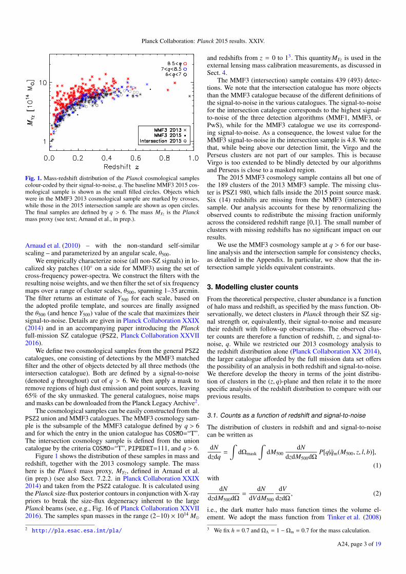
Fig. 1. Mass-redshift distribution of the Planck cosmological samplescolour-coded by their signal-to-noise, q. The baseline MMF3 2015 cos-mological sample is shown as the small filled circles. Objects whichwere in the MMF3 2013 cosmological sample are marked by crosses,while those in the 2015 intersection sample are shown as open circles.The final samples are defined by q > 6. The mass MYz is the Planckmass proxy (see text; Arnaud et al., in prep.).

Arnaud et al. (2010) – with the non-standard self-similarscaling – and parameterized by an angular scale, θ500.

We empirically characterize noise (all non-SZ signals) in lo-calized sky patches (10 on a side for MMF3) using the set ofcross-frequency power-spectra. We construct the filters with theresulting noise weights, and we then filter the set of six frequencymaps over a range of cluster scales, θ500, spanning 1–35 arcmin.The filter returns an estimate of Y500 for each scale, based onthe adopted profile template, and sources are finally assignedthe θ500 (and hence Y500) value of the scale that maximizes theirsignal-to-noise. Details are given in Planck Collaboration XXIX(2014) and in an accompanying paper introducing the Planckfull-mission SZ catalogue (PSZ2, Planck Collaboration XXVII2016).

We define two cosmological samples from the general PSZ2catalogues, one consisting of detections by the MMF3 matchedfilter and the other of objects detected by all three methods (theintersection catalogue). Both are defined by a signal-to-noise(denoted q throughout) cut of q > 6. We then apply a mask toremove regions of high dust emission and point sources, leaving65% of the sky unmasked. The general catalogues, noise mapsand masks can be downloaded from the Planck Legacy Archive2.

The cosmological samples can be easily constructed from thePSZ2 union and MMF3 catalogues. The MMF3 cosmology sam-ple is the subsample of the MMF3 catalogue defined by q > 6and for which the entry in the union catalogue has COSMO=“T”.The intersection cosmology sample is defined from the unioncatalogue by the criteria COSMO=“T”, PIPEDET=111, and q > 6.

Figure 1 shows the distribution of these samples in mass andredshift, together with the 2013 cosmology sample. The masshere is the Planck mass proxy, MYz, defined in Arnaud et al.(in prep.) (see also Sect. 7.2.2. in Planck Collaboration XXIX2014) and taken from the PSZ2 catalogue. It is calculated usingthe Planck size-flux posterior contours in conjunction with X-raypriors to break the size-flux degeneracy inherent to the largePlanck beams (see, e.g., Fig. 16 of Planck Collaboration XXVII2016). The samples span masses in the range (2−10) × 1014 M

2 http://pla.esac.esa.int/pla/

and redshifts from z = 0 to 13. This quantityMYz is used in theexternal lensing mass calibration measurements, as discussed inSect. 4.

The MMF3 (intersection) sample contains 439 (493) detec-tions. We note that the intersection catalogue has more objectsthan the MMF3 catalogue because of the different definitions ofthe signal-to-noise in the various catalogues. The signal-to-noisefor the intersection catalogue corresponds to the highest signal-to-noise of the three detection algorithms (MMF1, MMF3, orPwS), while for the MMF3 catalogue we use its correspond-ing signal-to-noise. As a consequence, the lowest value for theMMF3 signal-to-noise in the intersection sample is 4.8. We notethat, while being above our detection limit, the Virgo and thePerseus clusters are not part of our samples. This is becauseVirgo is too extended to be blindly detected by our algorithmsand Perseus is close to a masked region.

The 2015 MMF3 cosmology sample contains all but one ofthe 189 clusters of the 2013 MMF3 sample. The missing clus-ter is PSZ1 980, which falls inside the 2015 point source mask.Six (14) redshifts are missing from the MMF3 (intersection)sample. Our analysis accounts for these by renormalizing theobserved counts to redistribute the missing fraction uniformlyacross the considered redshift range [0,1]. The small number ofclusters with missing redshifts has no significant impact on ourresults.

We use the MMF3 cosmology sample at q > 6 for our base-line analysis and the intersection sample for consistency checks,as detailed in the Appendix. In particular, we show that the in-tersection sample yields equivalent constraints.

3. Modelling cluster counts

From the theoretical perspective, cluster abundance is a functionof halo mass and redshift, as specified by the mass function. Ob-servationally, we detect clusters in Planck through their SZ sig-nal strength or, equivalently, their signal-to-noise and measuretheir redshift with follow-up observations. The observed clus-ter counts are therefore a function of redshift, z, and signal-to-noise, q. While we restricted our 2013 cosmology analysis tothe redshift distribution alone (Planck Collaboration XX 2014),the larger catalogue afforded by the full mission data set offersthe possibility of an analysis in both redshift and signal-to-noise.We therefore develop the theory in terms of the joint distribu-tion of clusters in the (z, q)-plane and then relate it to the morespecific analysis of the redshift distribution to compare with ourprevious results.

3.1. Counts as a function of redshift and signal-to-noise

The distribution of clusters in redshift and and signal-to-noisecan be written as

dNdzdq

=

∫dΩmask

∫dM500

dNdzdM500dΩ

P[q|qm(M500, z, l, b)],

(1)

with

dNdzdM500dΩ

=dN

dVdM500

dVdzdΩ

, (2)

i.e., the dark matter halo mass function times the volume el-ement. We adopt the mass function from Tinker et al. (2008)

3 We fix h = 0.7 and ΩΛ = 1 −Ωm = 0.7 for the mass calculation.

A24, page 3 of 19

A&A 594, A24 (2016)

throughout, apart from the Appendix, where we compare to theWatson et al. (2013a) mass function as a test of modelling ro-bustness; there, we show that the Watson et al. (2013a) massfunction yields constraints similar to those from the Tinker et al.(2008) mass function, but shifted by about 1σ towards higher Ωmand lower σ8 along the main degeneracy line.

The quantity P[q|qm(M500, z, l, b)] is the distribution of qgiven the mean signal-to-noise value, qm(M500, z, l, b), predictedby the model for a cluster of mass M500 and redshift z lo-cated at Galactic coordinates (l, b) 4. This latter quantity is de-fined as the ratio of the mean SZ signal expected of a cluster,Y500(M500, z), as given in Eq. (7), and the detection filter noise,σf[θ500(M500, z), l, b]:

qm ≡ Y500(M500, z)/σf[θ500(M500, z), l, b]. (3)

The filter noise depends on sky location (l, b) and the clus-ter angular size, θ500, which introduces additional depen-dence on mass and redshift. More detail on σf can be foundin Planck Collaboration XX (2014) (see in particular Fig. 4therein).

The distribution P[q|qm] incorporates noise fluctuations andintrinsic scatter in the actual cluster Y500 around the mean value,Y500(M500, z), predicted from the scaling relation. We discuss thisscaling relation and our log-normal model for the intrinsic scatterbelow, and Sect. 4 examines the calibration of the overall massscale for the scaling relation.

The redshift distribution of clusters detected at q > qcat is theintegral of Eq. (1) over signal-to-noise,

dNdz

(q > qcat) =

∫ ∞

qcat

dqdN

dzdq

=

∫dΩ

∫dM500 χ(M500, z, l, b)

dNdzdM500dΩ

, (4)

with

χ(M500, z, l, b) =

∫ ∞

qcat

dq P[q|qm(M500, z, l, b)]. (5)

Equation (4) is equivalent to the expression used in our 2013analysis if we write it in the form

χ =

∫dln Y500

∫dθ500P(ln Y500, θ500|z,M500) χ(Y500, θ500, l, b),

(6)

where χ(Y500, θ500, l, b) is the survey selection function atq > qcat in terms of true cluster parameters (Sect. 3.3), andP(ln Y500, θ500|z,M500) is the distribution of these parametersgiven cluster mass and redshift. We specify the relation betweenEqs. (5) and (6) in the next section.

3.2. Observable-mass relations

A crucial element of our modelling is the relation between clus-ter observables, Y500 and θ500, and halo mass and redshift. Dueto intrinsic variations in cluster properties, this relation is de-scribed by a distribution function, P(ln Y500, θ500|M500, z), whosemean values are specified by the scaling relations Y500(M500, z)and θ500(M500, z).

4 This form assumes, as we do throughout, that the distribution de-pends on z and M500 only through the mean value qm, specifically, thatthe intrinsic scatter, σln Y , of Eq. (9) is constant.

Table 1. Summary of SZ-mass scaling-law parameters (see Eq. (7)).

Parameter Valuelog Y∗ −0.19 ± 0.02αa 1.79 ± 0.08βb 0.66 ± 0.50σln Y

c 0.173 ± 0.023

Notes. (a) Except when specified, α is constrained by this prior inour one-dimensional likelihood over N(z), but left free in our two-dimensional likelihood over N(z, q). (b) We fix β to its central valuethroughout, except when examining modelling uncertainties in the Ap-pendix. (c) The value is the same as in our 2013 analysis, given here interms of the natural logarithm and computed from σlog Y = 0.075±0.01.

We use the same form for these scaling relations as in our2013 analysis:

E−β(z) D2

A(z)Y500

10−4 Mpc2

= Y∗

[h

0.7

]−2+α [(1 − b) M500

6 × 1014 M

]α, (7)

and

θ500 = θ∗

[h

0.7

]−2/3 [(1 − b) M500

3 × 1014 M

]1/3

E−2/3(z)[

DA(z)500 Mpc

]−1

, (8)

where θ∗ = 6.997 arcmin, and fiducial ranges for the parame-ters Y∗, α, and β are listed in Table 1; these values are identi-cal to those used in our 2013 analysis. Unless otherwise stated,we use Gaussian distributions with mean and standard deviationgiven by these values as prior constraints; one notable exceptionwill be when we simultaneously fit for α and cosmological pa-rameters. In the above expressions, DA(z) is the angular diameterdistance and E(z) ≡ H(z)/H0.

These scaling relations have been established by X-ray ob-servations, as detailed in the Appendix of Planck Collabora-tion XX 2014, and rely on mass determinations, MX, based onhydrostatic equilibrium of the intra-cluster gas. The “mass bias”parameter, b, assumed to be constant in both mass and redshift,allows for any difference between the X-ray determined massesand true cluster halo mass: MX = (1 − b)M500. This is discussedat length in Sect. 4.

We adopt a log-normal5 distribution for Y500 around its meanvalue Y500, and a delta function for θ500 centred on θ500:

P(ln Y500, θ500|M500, z) =1

√2πσln Y

e− ln2(Y500/Y500)/(2σ2ln Y )

× δ[θ500 − θ500], (9)

where Y500(M500, z) and θ500(M500, z) are given by Eqs. (7)and (8). The δ-function maintains the empirical definition of R500that is used in observational determinations of the profile.

We can now specify the relation between Eqs. (5) and (6) bynoting that

P[q|qm(M500, z, l, b)] =

∫dln qmP[q|qm]P[ln qm|qm], (10)

where P[q|qm] is the distribution of observed signal-to-noise,q, given the model value, qm. The second distribution repre-sents intrinsic cluster scatter, which we write in terms of our

5 In this paper, “ln” denotes the natural logarithm and “log” the log-arithm to base 10; the expression is written in terms of the naturallogarithm.

A24, page 4 of 19

Planck Collaboration: Planck 2015 results. XXIV.

observable-mass distribution, Eq. (9), as

P[ln qm|qm] =

∫dθ500P[ln Y500(ln qm, θ500, l, b), θ500|M500, z]

=1

√2πσln Y

e− ln2(qm/qm)/2σ2ln Y . (11)

Performing the integral of Eq. (5), we find

χ =

∫dln qmP[ln qm|qm]χ(Y500, θ500, l, b), (12)

with the definition of our survey selection function

χ(Y500, θ500, l, b) =

∫ ∞

qcat

dqP[q|qm(Y500, θ500, l, b)]. (13)

We then reproduce Eq. (6) by using the first line of Eqs. (11)and (3).

3.3. Selection function and survey completeness

The fundamental quantity describing the survey selection isP[q|qm], introduced in Eq. (10). It gives the observed signal-to-noise, used to select SZ sources, as a function of model (“true”)cluster parameters through qm(Y500, θ500, l, b), and it defines the“survey selection function” χ(Y500, θ500, l, b) via Eq. (13). Wecharacterize the survey selection in two ways. The first is with ananalytical model and the second employs a Monte Carlo extrac-tion of simulated sources injected into the Planck maps. In addi-tion, we perform an external validation of our selection functionusing known X-ray clusters.

The analytical model assumes pure Gaussian noise, in whichcase we simply have P[q|qm] = e−(q−qm)2/2/

√2π. The survey se-

lection function is then given by the error function (and we referto this as the ERF completeness function),

χ(Y500, θ500, l, b) =12

[1 − erf

(qcat − qm(Y500, θ500, l, b)

√2

)]· (14)

This model can be applied to a catalogue with well-defined noiseproperties (i.e., σf), such as our MMF3 catalogue, but not to theintersection catalogue based on the simultaneous detection withthree different methods. This is our motivation for choosing theMMF3 catalogue as our baseline.

In the Monte Carlo approach, we inject simulated clustersdirectly into the Planck maps and (re)extract them with the com-plete detection pipeline. Details are given in the accompanying2015 SZ catalogue paper, Planck Collaboration XXVII (2016).This method provides a more comprehensive description of thesurvey selection by accounting for a variety of effects beyondnoise. In particular, we vary the shape of the SZ profile atfixed Y500 and θ500 to quantify its effect on catalogue complete-ness. The difference between the Monte-Carlo and ERF com-pleteness results in a change in modelled number counts of typ-ically ∼2.5% (with a maximum of 9%) in each redshift bin.

We also perform an external check of the survey complete-ness using known X-ray clusters from the Meta Catalogue ofX-ray Clusters (MCXC) compilation (Piffaretti et al. 2011) andalso SPT clusters from Bleem et al. (2015). Details are givenin the 2015 SZ catalogue paper, Planck Collaboration XXVII(2016). For the MCXC compilation, we rely on the expecta-tion that at redshifts z < 0.2 any Planck-detected cluster shouldbe found in one of the ROSAT catalogues (Chamballu et al.2012) because at low redshift ROSAT probes to lower masses

than Planck6. The MCXC catalogue provides a truth table, re-placing the input cluster list of the simulations, and we com-pute completeness as the ratio of objects in the cosmologycatalogue to the total number of clusters. As discussed inPlanck Collaboration XXVII (2016), the results are consistentwith Gaussian noise and bound the possible effect of profile vari-ations. We arrive at the same conclusion when applying the tech-nique to the SPT catalogue.

Planck Collaboration XXVII (2016) discusses completenesschecks in greater detail. One possible source of bias is thepresence of correlated IR emission from cluster member galax-ies. Planck Collaboration XXIII (2016) suggests that IR pointsources may contribute significantly to the cluster SED at thePlanck frequencies, especially at higher redshift. The potentialimpact of this effect warrants further study in future work.

We thus have different estimations of the selection functionfor MMF3 and the intersection catalogues. We test the sensi-tivity of our cosmological constraints to the selection functionin Appendix A by comparing results obtained with the differentmethods and catalogues. We find that our results are insensitiveto the choice of completeness model (Fig A.1), and we thereforeadopt the analytical ERF completeness function for simplicitythroughout the paper.

4. The cluster mass scale

The characteristic mass scale of our cluster sample is the criti-cal element in our analysis of the counts. It is controlled by themass bias factor, 1 − b, accounting for any difference betweenthe X-ray mass proxies used to establish the scaling relationsand the true (halo) mass: MX = (1 − b)M500. Such a differencecould arise from cluster physics (such as a violation of hydro-static equilibrium or temperature structure in the gas, Rasia et al.2006, 2012, 2014), from observational effects (e.g., instrumentalcalibration), or from selection effects biasing the X-ray samplesrelative to SZ- or mass-selected samples (Angulo et al. 2012).

In our 2013 analysis, we adopted a flat prior on the massbias over the range 1 − b = [0.7, 1.0], with a reference modeldefined by 1 − b = 0.8. This was motivated by a compari-son of the Y − MX relation with published Y − M relations de-rived from numerical simulations, as detailed in the Appendixof Planck Collaboration XX (2014); this estimate was consis-tent with most (although not all) predictions for any violationof hydrostatic equilibrium, as well as observational constraintsfrom the available lensing observations. Effects other than clus-ter physics can contribute to the mass bias, as discussed in ourearlier paper, and as emphasized by the survey of cluster multi-band scaling relations by Rozo et al. (2014a,b,c).

The mass bias was the largest uncertainty in our 2013 anal-ysis, and it severely hampered understanding of the tensionfound between constraints from the primary CMB and the clustercounts. Here, we incorporate new lensing mass determinations ofPlanck clusters to constrain the mass bias. We also apply a novelmethod to measure object masses based on lensing of CMB tem-perature anisotropies behind clusters (Melin & Bartlett 2015).These constraints are used as prior information in our analysisof the counts. As we will see, however, uncertainty in the massbias remains our largest source of uncertainty, mainly becausethese various determinations continue to differ by up to 30%.

6 In fact, this expectation is violated to a small degree. As discussedin Planck Collaboration XXVII (2016), there appears to be a small pop-ulation of X-ray under-luminous clusters.

A24, page 5 of 19

A&A 594, A24 (2016)

Table 2. Summary of mass scale priors.

Prior name Quantity Value and Gaussian errorsWeighing the Giants (WtG) 1 − b 0.688 ± 0.072Canadian Cluster ComparisonProject (CCCP) 1 − b 0.780 ± 0.092CMB lensing (CMBlens) 1/(1 − b) 0.99 ± 0.19Baseline 2013 1 − b 0.8 [−0.1,+0.2]

Notes. For CCCP, we use the value determined for Planck clusters atS/N > 7 (Hoekstra et al. 2015, left column of p. 706) and we addin quadrature the statistical (0.07) and systematic (0.06) uncertainties.CMB lensing directly measures 1/(1 − b), which we implement in ouranalysis; purely for reference, this constraint translates approximatelyto 1 − b = 1.01+0.24

−0.16. The last line shows the 2013 baseline – a referencemodel defined by 1 − b = 0.8 with a flat prior in the [0.7, 1] range.

In general, the mass bias could depend on cluster mass andredshift, although we will model it by a constant in the following.Our motivation is one of practicality: the limited size and preci-sion of current lensing samples makes it difficult to constrainany more than a constant value, i.e., the overall mass scale ofour catalogue. Large lensing surveys like Euclid, WFIRST, andthe Large Synoptic Survey Telescope, as well as CMB lensing,will improve this situation in coming years.

4.1. Constraints from gravitational shear

Several cluster samples with high quality gravitational shearmass measurements have appeared since 2013. Among these,the Weighing the Giants (WtG, von der Linden et al. 2014a),CLASH (Postman et al. 2012; Merten et al. 2015; Umetsu et al.2014), and Canadian Cluster Comparison Project (CCCP,Hoekstra et al. 2015) programmes offer constraints on our massbias factor, 1−b, through direct comparison of the lensing massesto the Planck mass proxy, MYz.

The analysis by the WtG programme of 22 clusters from the2013 Planck cosmology sample yields 1 − b = 0.688 ± 0.072.Their result lies at the very extreme of the range explored inPlanck Collaboration XX (2014) and would substantially reducethe tension found between primary CMB and galaxy cluster con-straints. Hoekstra et al. (2015) report a smaller bias of 1 − b =0.78 ± 0.07 (stat) ± 0.06 (sys) for a set of 20 common clusters,which is in good agreement with the fiducial value adopted inour 2013 analysis. In our new analysis we add the statistical andsystematic uncertainties in quadrature (see Table 2).

The two samples overlap, but not completely, and, as dis-cussed in detail by Hoekstra et al. (2015), there are numerousdifferences between the two analyses. These include treatment ofsource redshifts, contamination by cluster members and methodsof extracting a mass estimate from the lensing data. And whilethe two mass calibrations differ in a way that attracts particularattention in the present context, they are statistically consistent,separated by about one standard deviation.

4.2. Constraints from CMB lensing

Measuring cluster mass through CMB lensing (Lewis &Challinor 2006) has been discussed in the literature for sometime since the study performed by Zaldarriaga & Seljak (1999).We apply a new technique for measuring cluster masses throughlensing of CMB temperature anisotropies (Melin & Bartlett2015), allowing us to calibrate the scaling relations using only

Fig. 2. Cluster mass scale determined by CMB lensing. We show theratio of cluster lensing mass, Mlens, to the SZ mass proxy, MYz, as afunction of the mass proxy for clusters in the MMF3 2015 cosmologysample. The cluster mass is measured through lensing of CMB tempera-ture anisotropies in the Planck data (Melin & Bartlett 2015). Individualmass measurements have low signal-to-noise, but we determine a meanratio for the sample of Mlens/MYz = 1/(1 − b) = 0.99 ± 0.19. For clarity,only some of the error bars are plotted (see text).

Planck data. This is a valuable alternative to the galaxy lens-ing observations because it is independent and affected by dif-ferent possible systematics. Additionally, we can apply it to theentire cluster sample to obtain a mass calibration representativeof an SZ flux-selected sample. Similar approaches using CMBlensing to measure halo masses were recently applied by SPT(Baxter et al. 2015) and ACT (Madhavacheril et al. 2015).

Our method first extracts a clean CMB temperature map witha constrained internal linear combination (ILC) of the Planckfrequency channels in the region around each cluster; the ILC isconstrained to nullify the SZ signal from the clusters themselvesand provide a clean CMB map of 5 arcmin resolution. Using aquadratic estimator on the CMB map, we reconstruct the lensingpotential in the field and then filter it to obtain an estimate of thecluster mass. The filter is an NFW profile (Navarro et al. 1997)with scale radius set by the Planck mass proxy for each clus-ter, and designed to return an estimate of the ratio Mlens/MYz,where MYz is the Planck SZ mass proxy. These individual mea-surements are corrected for any mean-field bias by subtractingidentical filter measurements on blank fields; this accounts foreffects of apodization over the cluster fields and correlated noise.The technique has been tested on realistic simulations of Planckfrequency maps. More detail can be found in Melin & Bartlett(2015).

Figure 2 shows Mlens/MYz as a function of MYz for all clus-ters in the MMF3 cosmology sample. Each point is an individualcluster7. For clarity, only some of the error bars on the ratio areshown; the error bars vary from 1.8 at the high mass end to 8.5at the low mass end, with a median of 4.2. There is no indicationof a correlation between the ratio and MYz, and we therefore fitfor a constant ratio of Mlens/MYz by taking the weighted mean(using the individual measurement uncertainties as provided bythe filter) over the full data set. If the ratio differs from unity,we apply a correction to account for the fact that our filter aper-ture was not perfectly matched to the clusters. The correction is

7 The values can be negative due to noise fluctuations and the lowsignal-to-noise of the individual measurements.

A24, page 6 of 19

Planck Collaboration: Planck 2015 results. XXIV.

calculated assuming an NFW profile and is of the order of onepercent.

The final result is 1/(1− b) = 0.99± 0.19, traced by the blueband in the figure. We note that the method constrains 1/(1 − b)rather than 1 − b as in the case of the shear measurements.The calculated uncertainty on the weighted mean is consistentwith a bootstrap analysis, where we create new catalogues of thesame size as the original by sampling objects from the full cat-alogue with replacement; the uncertainty from the bootstrap isthen taken as the standard deviation of the bootstrap means.

The uncertainty 0.19 is statistical. Melin & Bartlett (2015)quote an uncertainty of 0.28 for the 62 ESZ-XMM clustersbased on simulations including only tSZ, kSZ, primary CMBand instrumental noise. Scaling this number to 433 (numberof objects with a redshift in the cosmological sample) gives0.28√

62/433 ≈ 0.11, in broad agreement with our value of 0.19.The difference can likely be attributed to the fact that the Planckcosmological sample is on average less massive than the ESZ-XMM sample, and that the Planck maps are more complex thanthe model adopted in Melin & Bartlett (2015).

We have obtained a 5σ measurement of the sample massscale using CMB lensing. We emphasize, however, that themethod is new and under development. A number of potentialsystematic effects require further study, including cluster mis-centring and mismatch between filter shape and actual clusterprofiles; these would tend to reduce the observed masses fromtheir true values. On the other hand, effects such as contributionsfrom mass correlated on large scales with the clusters (e.g., fila-ments or neighbouring halos) and contamination by infrared andradio sources could increase the observed signal. We are exam-ining these issues in a study of the ESZ-XMM sample that willbe published at a later date.

4.3. Summary

The three mass bias priors are summarized in Table 2, and wewill extract cosmological constraints from each one. We favourthese three lensing results because of their direct comparisonto the Planck mass proxy. We will assume Gaussian distribu-tions for 1 − b (gravitational shear) or 1/(1 − b) (CMB lensing),with standard deviations given by the error column. We adopt theCCCP mass calibration as our baseline, and give the CMB lens-ing result less weight in our interpretation because of its noveltyand the ongoing studies of the issues mentioned in the previoussection.

5. Analysis methodology

5.1. Likelihood

Our 2013 analysis employed a likelihood built on the cluster red-shift distribution, dN/dz. With the larger 2015 catalogue, ourbaseline likelihood is now constructed on counts in the (z, q)-plane. We divide the catalogue into bins of size ∆z = 0.1(10 bins) and ∆log q = 0.25 (5 bins), each with an observed num-ber N(zi, q j) = Ni j of clusters. Modelling the observed counts,Ni j, as independent Poisson random variables, our log-likelihoodis

ln L =

NzNq∑i, j

[Ni j ln Ni j − Ni j − ln[Ni j!]

], (15)

where Nz and Nq are the total number of redshift and signal-to-noise bins, respectively. The mean number of objects in each bin

is predicted by theory according to Eq. (1):

Ni j =dN

dzdq(zi, q j)∆z∆q, (16)

which depends on the cosmological (and cluster modelling)parameters. In practice, we use a Monte Carlo Markov chain(MCMC) to map the likelihood surface around the maximumand establish confidence limits.

Equation (15) assumes that the bins are uncorrelated, whilea more complete description would include correlations due tolarge-scale clustering. In practice, our cluster sample containsmostly high mass systems for which the impact of these effectsis weak (e.g., Hu & Kravtsov 2003, in particular their Fig. 4 forthe impact on constraints in the (Ωm,σ8) plane).

5.2. External data sets

Cluster counts cannot constrain all pertinent cosmological pa-rameters; they are most sensitive to Ωm and σ8, and whenanalysing the counts alone we must apply additional obser-vational constraints as priors on other parameters. For thispurpose, we adopt Big Bang nucleosynthesis (BBN) con-straints from Steigman (2008), Ωbh2 = 0.022 ± 0.002 (fora recent review on BBN, see Olive 2013), and constraintsfrom baryon acoustic oscillations (BAO). The latter com-bine the 6dF Galaxy Survey (Beutler et al. 2011), the SDSSMain Galaxy Sample (Padmanabhan et al. 2012; Anderson et al.2012) and the BOSS DR11 (Anderson et al. 2014). We re-fer the reader to Sect. 5.2 in Planck Collaboration XIII (2016)for details of the combination. We also include a prior on nsfrom Planck Collaboration XVI (2014), ns = 0.9624 ± 0.014.When explicitly specified in the text, we add the supernovæ con-straint from SNLS-II and SNLS3: the Joint Light-curve Analysisconstraint (JLA, Betoule et al. 2014). The BAO are particularlysensitive to H0, while the supernovæ allow precise constraintson the dark energy equation-of-state parameter, w.

6. Comparison to 2013

We begin by verifying consistency with the results ofPlanck Collaboration XX (2014) (Sect. 6.1) based on the one-dimensional likelihood over the redshift distribution, dN/dz(Eq. (4)). We then examine the effect of changing to the full two-dimensional likelihood, dN/dzdq (Eq. (1)) in Sect. 6.2. For thispurpose we compare constraints on the total matter density, Ωm,and the linear-theory amplitude of the density perturbations to-day, σ8, using the cluster counts in combination with externaldata and fixing the mass bias. The two-dimensional likelihooddN/dzdq is then adopted as the baseline in the rest of the paper.

6.1. Constraints on Ωm and σ8: one-dimensional analysis

Figure 3 presents constraints from the MMF3 cluster countscombined with the BAO and BBN priors of Sect. 5.2; we re-fer to this data combination as “SZ+BAO+BBN”. To compareto results from our 2013 analysis (the grey, filled ellipses), weuse a one-dimensional likelihood based on Eq. (4) over the red-shift distribution and have adopted the reference scaling rela-tion of 2013, i.e., Eqs. (7) and (8), with the mass bias valuefixed to 1 − b = 0.8. For the present comparison, we usethe updated BAO constraints discussed in Sect. 5.2; these are

A24, page 7 of 19

A&A 594, A24 (2016)

0.25 0.30 0.35 0.40Ωm

0.70

0.74

0.78

0.82

σ8

PSZ2, q=6PSZ2, q=7PSZ2, q=8.5PSZ1, q=7

Fig. 3. Contours at 95% for different signal-to-noise thresholds, q =8.5, 7, and 6, applied to the 2015 MMF3 cosmology sample for theSZ+BAO+BBN data set. The contours are compatible with the 2013constraints (Planck Collaboration XX 2014), shown as the filled, lightgrey ellipses at 68 and 95% (for the BAO and BBN priors of Sect 5.2;see text). The 2015 catalogue thresholded at q > 8.5 has a similar num-ber of clusters (190) as the 2013 catalogue (189). This comparison ismade using the analytical error-function model for completeness andadopts the reference observable-mass scaling relation of the 2013 anal-ysis (1 − b = 0.8, see text). The redshift distributions of the best-fitmodels are shown in Fig. 4. For this figure and Fig. 4, we use the one-dimensional likelihood over the redshift distribution, dN/dz (Eq. (4)).

stronger than the BAO constraints used in the 2013 analysis, andthe grey contours shown here are consequently smaller than inPlanck Collaboration XX (2014).

Limiting the 2015 catalogue to q > 8.5 produces a sam-ple with 190 clusters, similar to the 2013 cosmology catalogue(189 objects). The two sets of constraints demonstrate good con-sistency, and they remain consistent while becoming tighter aswe decrease the signal-to-noise threshold of the 2015 catalogue.Under similar assumptions, our 2015 analysis thus confirms the2013 results reported in Planck Collaboration XX (2014).

The area of the ellipse from q = 8.5 to q = 6 decreases by afactor of 1.3. This is substantially less than the factor of 2.3 ex-pected from the ratio of the number of objects in the two sam-ples. The difference may be related to the decreasing goodness-of-fit of the best model as the signal-to-noise decreases. Whenincorporated, the uncertainty on the mass calibration 1 − b willalso restrict the reduction of the ellipse area.

Figure 4 overlays the observed cluster redshift distributionon the predictions from the best-fit model in each case. We seethat the models do not match the counts in the second and thirdredshift bins (counting from z = 0), and that the discrepancy,already marginally present at the high signal-to-noise cut cor-responding to the 2013 catalogue, becomes more pronouncedtowards the lower signal-to-noise thresholds. This discrepancycannot be attributed to redshift errors in the first bins becausethe majority of the redshifts are spectroscopic and the size ofthe bins is large (∆z = 0.1); for example, the first two redshiftbins contain 208 clusters, of which 200 have spectroscopic red-shifts. The dependence on signal-to-noise may suggest that thedata prefer a different slope, α, of the scaling relation than al-lowed by the prior of Table 1. We explore the effect of relaxingthe X-ray prior on α in the next section.

0.0 0.2 0.4 0.6 0.8 1.0z

020

4060

8010

012

014

0N

(z)

best fit q=6best fit q=7best fit q=8.5MMF3 q=6MMF3 q=7MMF3 q=8.5

Fig. 4. Comparison of observed counts (points with error bars) with pre-dictions of the best-fit models (solid lines) from the one-dimensionallikelihood for three different thresholds applied to the 2015 MMF3 cos-mology sample. The mismatch between observed and predicted countsin the second and third lowest redshift bins, already noticed in the 2013analysis, increases at lower thresholds, q. The best-fit models are de-fined by the constraints shown in Fig. 3. For this figure and Fig. 3, weuse our one-dimensional likelihood over the redshift distribution, dN/dz(Eq. (4)), with the mass biased fixed at (1 − b) = 0.8.

6.2. Constraints on Ωm and σ8: two-dimensional analysis

In Fig. 5 we compare constraints from the one- and two-dimensional likelihood with α either free or with the priorof Table 1. For this comparison, we continue with the“SZ+BAO+BBN” data set, but adopt the CCCP prior for themass bias and only consider the full 2015 MMF3 catalogue atq > 6.

The grey and black contours and lines in Fig. 5 show resultsfrom the one-dimensional likelihood fit to the redshift distribu-tion using, respectively, the X-ray prior on α and leaving α free.The redshift counts do indeed prefer a steeper slope, with a pos-terior of α = 2.23 ± 0.18 in the latter case and a shift of theconstraints along their degeneracy ridges. To explore this pref-erence, we split the analysis into low and high redshift bin setsdivided at z = 0.2, finding that neither the high nor the low red-shift bin set prefers the steeper slope by itself; it appears onlywhen analyzing all the bins. As described further in Appendix A,there is a subtle interplay between parameters that is maskedby the degeneracies and difficult to interpret with the presentdata set.

A related issue is the acceptability of the model fit. Wedefine a generalized χ2 measure of goodness-of-fit as χ2 =∑Nz

i N−1i

(Ni − Ni

)2, determining the probability to exceed (PTE)

the observed value using Monte Carlo simulations of Poissonstatistics for each bin with the best-fit model mean Ni. The ob-served value of the fit drops from 17 (PTE = 0.07) with the X-rayprior, to 15 (PTE = 0.11) when leaving α free. When leaving αfree, Ωm increases and σ8 decreases, following their correlationwith α shown by the contours, and their uncertainty increasesdue to the added parameter.

The two-dimensional likelihood over dN/dzdq better con-strains the slope when α is free, as shown by the violet curvesand contours. In this case, the preferred value drops back towardsthe X-ray prior: α = 1.89 ± 0.11, just over 1σ from the centralX-ray value. Re-imposing the X-ray prior on α with the two-dimensional likelihood (blue curves) does little to change the

A24, page 8 of 19

Planck Collaboration: Planck 2015 results. XXIV.

0.25 0.31 0.38 0.44

N(z,q) α freeN(z,q) α constrainedN(z) α freeN(z) α constrained

0.25 0.31 0.38 0.44

1.7

2.1

2.5

α

1.7 2.1 2.5

0.25 0.31 0.38 0.44

0.65

0.75

0.85

σ8

1.7 2.1 2.5 0.65 0.75 0.85

0.25 0.31 0.38 0.44Ωm

6267

7277

H0

1.7 2.1 2.5α

0.65 0.75 0.85σ8

62 67 72 77H0

Fig. 5. Comparison of constraints from the one-dimensional (dN/dz)and two-dimensional (dN/dzdq) likelihoods on cosmological param-eters and the scaling relation mass exponent, α. This comparisonuses the MMF3 catalogue, the CCCP prior on the mass bias and theSZ+BAO+BBN data set. The corresponding best-fit model redshift dis-tributions are shown in Fig. 6.

0.0 0.2 0.4 0.6 0.8 1.0z

020

4060

8010

012

014

016

0N

(z)

N(z,q) best fit (CCCP, α constrained)N(z,q) best fit (CCCP, α free)N(z) best fit (CCCP, α constrained)N(z) best fit (CCCP, α free)observed counts

Fig. 6. Redshift distribution of best-fit models from the four analysiscases shown in Fig. 5. The observed counts in the MMF3 catalogue(q > 6) are plotted as the red points with error bars, and as in Fig. 5 weadopt the CCCP mass prior with the SZ+BAO+BBN data set.

parameter constraints. Although the one-dimensional likelihoodprefers a steeper slope than the X-ray prior, the two-dimensionalanalysis does not, and the cosmological constraints remain ro-bust to varying α.

We define a generalized χ2 statistic as described above, nowover the two-dimensional bins in the (z, q)-plane. This general-ized χ2 for the fit with the X-ray prior is 43 (PTE = 0.28), com-pared to χ2 = 45 (PTE = 0.23) when α is a free parameter.

Figure 6 displays the redshift distribution of the best-fit mod-els in all four cases. Despite their apparent difficulty in match-ing the second and third redshift bins, the PTE values suggestthat these fits are moderately good to acceptable. We note that,as mentioned briefly in Sect. 5.1, clustering effects will increasethe scatter in each bin slightly over the Poisson value we have as-sumed, causing our quoted PTE values to be somewhat smallerthan the true ones.

0.25 0.30 0.35 0.40 0.45 0.50 0.55Ωm

0.60

0.68

0.76

0.84

0.92

σ8

CMBSZ+Lensing PSCMB+BAOSZα+BAO (WtG)SZα+BAO (CCCP)SZα+BAO (CMBlens)

Fig. 7. Comparison of constraints from the CMB to those from the clus-ter counts in the (Ωm, σ8)-plane. The green, blue and violet contoursgive the cluster constraints (two-dimensional likelihood) at 68 and 95%for the WtG, CCCP, and CMB lensing mass calibrations, respectively,as listed in Table 2. These constraints are obtained from the MMF3 cata-logue with the SZ+BAO+BBN data set and α free (hence the SZα nota-tion). Constraints from the Planck TT, TE, EE+lowP CMB likelihood(hereafter, Planck primary CMB) are shown as the dashed contoursenclosing 68 and 95% confidence regions (Planck Collaboration XIII2016), while the grey shaded region also includes BAO. The redcontours give results from a joint analysis of the cluster counts andthe Planck lensing power spectrum (Planck Collaboration XV 2016),adopting our external priors on ns and Ωbh2 with the mass bias param-eter free and α constrained by the X-ray prior (hence the SZ notationwithout the subscript α).

7. Cosmological constraints 2015

We extract constraints on Ωm and σ8 from the cluster counts incombination with external data, imposing the different clustermass scale calibrations as prior distributions on the mass bias.In Sect. 7.1, we compare our new constraints to and then com-bine them with those from the CMB anisotropies in the baseΛCDM model. We study parameter extensions to the base modelin Sect. 7.2. In the following, we adopt as our baseline the 2015two-dimensional SZ likelihood with the CCCP mass bias prior,α free and β = 2/3 fixed in Eq. (7). All quoted intervals are 68%confidence and all upper/lower limits are 95% confidence.

7.1. Base ΛCDM

7.1.1. Constraints on Ωm and σ8: comparison to primaryCMB parameters

Our 2013 analysis brought to light tension between constraintson Ωm andσ8 from the cluster counts and those from the primaryCMB in the base ΛCDM model. In that analysis, we adopted aflat prior on the mass bias over the range 1−b = [0.7, 1.0], with areference model defined by 1−b = 0.8 (see discussion in the Ap-pendix of Planck Collaboration XX 2014). Given the good con-sistency between the 2013 and 2015 cluster results (Fig. 3), weexpect the tension to remain under the same assumptions con-cerning the mass bias.

Figure 7 compares our 2015 cluster constraints (MMF3SZ+BAO+BBN) to those for the base ΛCDM model from thePlanck CMB anisotropies. The cluster constraints, given thethree different priors on the mass bias, are shown by the filledcontours at 68 and 95% confidence, while the dashed black

A24, page 9 of 19

A&A 594, A24 (2016)

Table 3. Summary of Planck 2015 cluster cosmology constraints

Data σ8

(Ωm0.31

)0.3Ωm σ8

WtG + BAO + BBN 0.806 ± 0.032 0.34 ± 0.03 0.78 ± 0.03CCCP + BAO + BBN [Baseline] 0.774 ± 0.034 0.33 ± 0.03 0.76 ± 0.03CMBlens + BAO + BBN 0.723 ± 0.038 0.32 ± 0.03 0.71 ± 0.03CCCP + H0 + BBN 0.772 ± 0.034 0.31 ± 0.04 0.78 ± 0.04

Notes. The constraints are obtained for our baseline model: the two-dimensional likelihood over the MMF3 catalogue (q > 6) with α free andβ = 2/3 fixed in Eq. (7).

contours give the Planck TT,TE,EE+lowP constraints (hereafterPlanck primary CMB, Planck Collaboration XIII 2016); the greyshaded regions add BAO to the CMB. The central value of theWtG mass prior lies at the extreme end of the range used in2013 (i.e., 1 − b = 0.7); with its uncertainty range extendingeven lower, the tension with primary CMB is greatly reduced, aspointed out by von der Linden et al. (2014b). With similar un-certainty but a central value shifted to 1 − b = 0.78, the CCCPmass prior results in greater tension with the primary CMB. Thelensing mass prior, finally, implies little bias and hence muchgreater tension.

The red contours present results from a joint analysis ofthe cluster counts and the Planck lensing power spectrum(Planck Collaboration XV 2016), adopting our external priors onns and Ωbh2 with the mass bias parameter free and α constrainedby the X-ray prior. It is interesting to note that these constraintsare fully independent of those from the primary CMB, but are ingood agreement with them, favouring only slightly lower valuesfor σ8.

Table 3 summarizes our cluster cosmology constraints for thebase ΛCDM model for the different mass bias priors. We givethe marginalized constraints on Ωm and σ8, as well as their com-bination that is most tightly constrained by the cluster counts.In addition, in the last line we list constraints when replacingthe BAO prior by a prior on H0 from direct local measurements(Riess et al. 2011): H0 = 73.8 ± 2.4 km s−1 Mpc−1.

7.1.2. Joint Planck 2015 primary CMB and clusterconstraints

Mass bias required by the primary CMB. In Fig. 8 we comparethe three prior distributions to the mass bias required by the pri-mary CMB. The latter is obtained as the posterior on 1−b from ajoint analysis of the MMF3 cluster counts and the CMB with themass bias as a free parameter. The best-fit value in this case is1 − b = 0.58 ± 0.04, more than 1σ below the central WtG value.Perfect agreement with the primary CMB would imply that clus-ters are even more massive than the WtG calibration. This figuremost clearly quantifies the tension between the Planck clustercounts and primary CMB.

Reionization optical depth. Primary CMB temperatureanisotropies also provide a precise measurement of the param-eter combination Ase−2τ, where τ is the optical depth fromThomson scatter after reionization and As is the power spectrumnormalization on large scales (Planck Collaboration XIII 2016).Low-` polarization anisotropies break the degeneracy by con-straining τ itself, but this measurement is delicate given the lowsignal amplitude and difficult systematic effects; it is important,however, in the determination of σ8. It is therefore interestingto compare the Planck primary CMB constraints on τ to thosefrom a joint analysis of the cluster counts and primary CMB

0.4 0.6 0.8 1.0 1.2 1.4 1.61−b

0.0

0.2

0.4

0.6

0.8

1.0

Pro

babili

ty d

ensi

ty

CMB+SZprior CCCPprior WtGprior CMBlens

Fig. 8. Comparison of cluster and primary CMB constraints in the baseΛCDM model, expressed in terms of the mass bias, 1 − b. The solidblack curve shows the distribution of values required to reconcile thecounts and primary CMB in ΛCDM; it is found as the posterior on 1−bfrom a joint analysis of the Planck cluster counts and primary CMBwhen leaving the mass bias free. The coloured dashed curves show thethree prior distributions on the mass bias listed in Table 2.

without the low-` polarization data (lowP). Battye et al. (2015),for instance, pointed out that a lower value for τ than suggestedby WMAP could reduce the level of tension between CMB andlarge-scale structure.

The comparison is shown in Fig. 9. We see that the PlanckTT + SZ constraints are in good agreement with the value fromPlanck CMB (i.e., TT,TE,EE+lowP), with the preferred valuefor WtG slightly higher and CMB lensing pushing towards alower value. The ordering CMB lensing/CCCP/WtG from lowerto higher τ posterior values matches the decreasing level of ten-sion with the primary CMB on σ8. These values remain, how-ever, larger than what is required to fully remove the tensionin each case. The posterior distributions for the mass bias are1− b = 0.60± 0.042, 1− b = 0.61± 0.049, 1− b = 0.66± 0.045,respectively, for WtG, CCCP and CMB lensing, all significantlyshifted from the corresponding priors of Table 2. Allowing τ toadjust offers only minor improvement in the tension reflectedby Fig. 8. Interestingly, the Planck TT posterior shown in Fig. 8of Planck Collaboration XIII (2016) peaks at significantly highervalues, while our Planck TT + SZ constraints are consistent withthe result from Planck TT + lensing, an independent constrainton τ without lowP.

7.2. Model extensions

7.2.1. Curvature

We consider constraints on spatial curvature that can be set bycluster counts. Our cluster counts combined with BBN and BAO

A24, page 10 of 19

Planck Collaboration: Planck 2015 results. XXIV.

0.05 0.10 0.15 0.20τ

0.0

0.2

0.4

0.6

0.8

1.0

Pro

babili

ty d

ensi

ty

CMB TT+EE+TE+lowPCMB TT+SZ (CCCP)CMB TT+SZ (WtG)CMB TT+SZ (CMBlens)

Fig. 9. Constraints on the reionization optical depth, τ. The dashed blackcurve is the constraint from Planck CMB (i.e., TT,TE,EE+lowP), whilethe three coloured lines are the posterior distribution on τ from a jointanalysis of the cluster counts and Planck TT only for the three differentmass bias parameters.

for the CCCP mass prior yield ΩK = −0.06 ± 0.06. This is com-pletely independent of the CMB, but consistent with the CMBplus BAO constraint of ΩK = 0.000 ± 0.002.

7.2.2. Dark energy

Constraints on dark energy and modified gravity based onPlanck CMB and external data sets are studied in detailin Planck Collaboration XIV (2016). In Fig. 10 we examine con-straints on a constant dark energy equation-of-state parameter, w.Analysis of the primary CMB alone results in the highly degen-erate grey contours. The degeneracy is broken by adding con-straints such as BAO (blue contours) or supernovae distances(rose-colored contours), both picking values around w = −1.The SZ counts (two-dimensional likelihood with CCCP prior)only marginally break the degeneracy when combined with theCMB, but when combined with BAO they do yield interestingconstraints (green contours) that are consistent with the inde-pendent constraints from the primary CMB combined with su-pernovae. We obtain Ωm = 0.314 ± 0.026 and w = −1.01 ± 0.18for SZ+BAO, Ωm = 0.306 ± 0.013 and w = −1.10 ± 0.06 forCMB+BAO, and Ωm = 0.306 ± 0.015 and w = −1.10 ± 0.05 forCMB+JLA.

7.2.3.∑

mν

An important, well-motivated extension to the base ΛCDMmodel that clusters can help constrain is a non-minimal sumof neutrino masses,

∑mν > 0.06 eV. Given the primary CMB

anisotropies, the amplitude of the density perturbations today,characterized by the equivalent linear theory extrapolation, σ8,is model dependent; it is a derived parameter, depending, for ex-ample, on the composition of the matter content of the Universe.Cluster abundance, on the other hand, provides a direct measure-ment of σ8 at low redshifts, and comparison to the value derivedfrom the CMB tests the adopted cosmological model.

By free-streaming, neutrinos damp the growth of matter per-turbations. Our discussion thus far has assumed the minimummass for the three known neutrino species. Increasing their mass,∑

mν > 0.06 eV, lowers σ8 because the neutrinos have largergravitational influence on the total matter perturbations. This

0.15 0.20 0.25 0.30 0.35 0.40Ωm

2.0

1.5

1.0

0.5

w

SZ+BAOCMBCMB+BAOCMB+JLA

Fig. 10. Constraints on a constant dark energy equation-of-state param-eter, w. Analysis of the primary CMB alone yields the grey contours thatare highly degenerate. Adding either BAO or supernovae to the CMBbreaks the degeneracy, giving constraints around w = −1. The greencontours are constraints from joint analysis of the SZ counts and BAO;although much less constraining they agree with the CMB+JLA com-binations and are completely independent.

goes in the direction of reconciling tension – the strength ofwhich depends on the mass bias – between the cluster and pri-mary CMB constraints. Cluster abundance, or any measure of σ8at low redshift, is therefore an important cosmological constraintto be combined with those from the primary CMB.

Figure 11 presents a joint analysis of the cluster counts forthe CCCP mass bias prior with primary CMB, the Planck lens-ing power spectrum, and BAO. The results without BAO (greenand red shaded contours) allow relatively large neutrino masses,up to

∑mν ≈ 0.5 eV; and when adding the lensing power spec-

trum, a small, broad peak appears in the posterior distributionjust above

∑mν = 0.2 eV. We also notice some interesting cor-

relations: the amplitude, σ8, anti-correlates with neutrino mass,as does the Hubble parameter, and larger values of α correspondto larger neutrino mass, lower H0, and lower σ8.

As discussed in detail in Planck Collaboration XIII (2016),the anti-correlation with the Hubble parameter maintains theobserved acoustic peak scale in the primary CMB. Increasingneutrino mass to simultaneously accommodate the cluster andprimary CMB constraints by lowering σ8, while allowed inthis joint analysis, would therefore necessarily increase ten-sion with most direct measurements of H0 (see discussionin Planck Collaboration XIII 2016). Including the BAO datagreatly restricts this possibility, as shown by the solid and dashedblack curves.

The solid and dashed, red and black curves in Fig. 12 re-produce the marginalized posterior distributions on

∑mν from

Fig. 11. The solid blue curve is the result of a similar analy-sis (CMB+SZ) where, in addition, the artificial parameter ALis allowed to vary. This parameter characterizes the amount oflensing in the temperature power spectrum relative to the bestfit model (Planck Collaboration XIII 2016). Planck TT+lowPalone constrains

AL = 1.22 ± 0.10,

which is in mild tension with the value predicted for the ΛCDMmodel, AL = 1. In the base ΛCDM model, this parameter isfixed to unity, but it is important to note that it is degener-ate with

∑mν. Left free, it allows less lensing power, which is

A24, page 11 of 19

A&A 594, A24 (2016)

0.31 0.35 0.39

CMB+SZCMB+SZ+lensingCMB+SZ+BAOCMB+SZ+lensing+BAO

0.31 0.35 0.39

0.65

0.73

0.81

0.89

σ8

0.65 0.73 0.81 0.89

0.31 0.35 0.39

0.55

0.65

0.75

1−b

0.65 0.73 0.81 0.89 0.55 0.65 0.75

0.31 0.35 0.39

1.7

1.8

1.9

2.0

α

0.65 0.73 0.81 0.89 0.55 0.65 0.75 1.7 1.8 1.9 2.0

0.31 0.35 0.39

0.1

0.3

0.5

0.7

Σmν[e

V]

0.65 0.73 0.81 0.89 0.55 0.65 0.75 1.7 1.8 1.9 2.0 0.1 0.3 0.5 0.7

0.27 0.31 0.35 0.39

Ωm

6266

70

H0

0.65 0.73 0.81 0.89

σ8

0.55 0.65 0.75

1−b

1.7 1.8 1.9 2.0

α

0.1 0.3 0.5 0.7

Σmν [eV]

62 66 70

H0

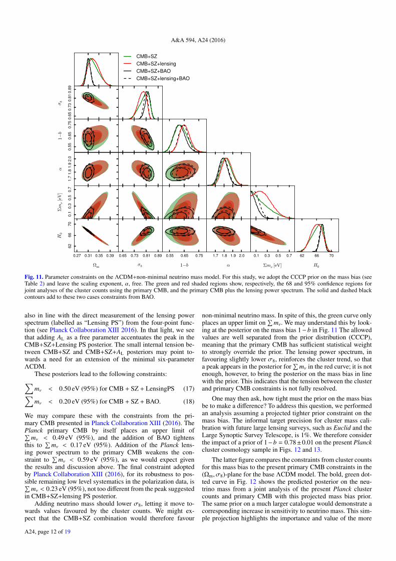
Fig. 11. Parameter constraints on the ΛCDM+non-minimal neutrino mass model. For this study, we adopt the CCCP prior on the mass bias (seeTable 2) and leave the scaling exponent, α, free. The green and red shaded regions show, respectively, the 68 and 95% confidence regions forjoint analyses of the cluster counts using the primary CMB, and the primary CMB plus the lensing power spectrum. The solid and dashed blackcontours add to these two cases constraints from BAO.

also in line with the direct measurement of the lensing powerspectrum (labelled as “Lensing PS”) from the four-point func-tion (see Planck Collaboration XIII 2016). In that light, we seethat adding AL as a free parameter accentuates the peak in theCMB+SZ+Lensing PS posterior. The small internal tension be-tween CMB+SZ and CMB+SZ+AL posteriors may point to-wards a need for an extension of the minimal six-parameterΛCDM.

These posteriors lead to the following constraints:∑mν < 0.50 eV (95%) for CMB + SZ + LensingPS (17)∑mν < 0.20 eV (95%) for CMB + SZ + BAO. (18)

We may compare these with the constraints from the pri-mary CMB presented in Planck Collaboration XIII (2016). ThePlanck primary CMB by itself places an upper limit of∑

mν < 0.49 eV (95%), and the addition of BAO tightensthis to

∑mν < 0.17 eV (95%). Addition of the Planck lens-

ing power spectrum to the primary CMB weakens the con-straint to

∑mν < 0.59 eV (95%), as we would expect given

the results and discussion above. The final constraint adoptedby Planck Collaboration XIII (2016), for its robustness to pos-sible remaining low level systematics in the polarization data, is∑

mν < 0.23 eV (95%), not too different from the peak suggestedin CMB+SZ+lensing PS posterior.

Adding neutrino mass should lower σ8, letting it move to-wards values favoured by the cluster counts. We might ex-pect that the CMB+SZ combination would therefore favour

non-minimal neutrino mass. In spite of this, the green curve onlyplaces an upper limit on

∑mν. We may understand this by look-

ing at the posterior on the mass bias 1− b in Fig. 11 The allowedvalues are well separated from the prior distribution (CCCP),meaning that the primary CMB has sufficient statistical weightto strongly override the prior. The lensing power spectrum, infavouring slightly lower σ8, reinforces the cluster trend, so thata peak appears in the posterior for

∑mν in the red curve; it is not

enough, however, to bring the posterior on the mass bias in linewith the prior. This indicates that the tension between the clusterand primary CMB constraints is not fully resolved.

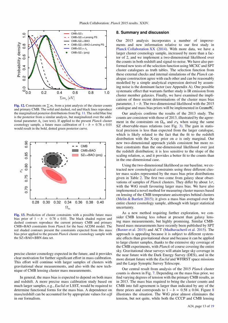
One may then ask, how tight must the prior on the mass biasbe to make a difference? To address this question, we performedan analysis assuming a projected tighter prior constraint on themass bias. The informal target precision for cluster mass cali-bration with future large lensing surveys, such as Euclid and theLarge Synoptic Survey Telescope, is 1%. We therefore considerthe impact of a prior of 1−b = 0.78±0.01 on the present Planckcluster cosmology sample in Figs. 12 and 13.

The latter figure compares the constraints from cluster countsfor this mass bias to the present primary CMB constraints in the(Ωm, σ8)-plane for the base ΛCDM model. The bold, green dot-ted curve in Fig. 12 shows the predicted posterior on the neu-trino mass from a joint analysis of the present Planck clustercounts and primary CMB with this projected mass bias prior.The same prior on a much larger catalogue would demonstrate acorresponding increase in sensitivity to neutrino mass. This sim-ple projection highlights the importance and value of the more

A24, page 12 of 19

Planck Collaboration: Planck 2015 results. XXIV.

0.0 0.2 0.4 0.6 0.8 1.0Σmν [eV]

0.0

0.2

0.4

0.6

0.8

1.0

Pro

babili

ty d

ensi

ty

CMB+SZαCMB+SZα+Lensing PSCMB+SZα+BAOCMB+SZα+BAO+Lensing PSCMB+SZα+AL

CMB+SZα (proj)

Fig. 12. Constraints on∑

mν from a joint analysis of the cluster countsand primary CMB. The solid and dashed, red and black lines reproducethe marginalized posterior distributions from Fig. 11. The solid blue lineis the posterior from a similar analysis, but marginalized over the addi-tional parameter AL (see text). If applied to the present Planck clustercosmology sample, a future mass calibration of 1 − b = 0.78 ± 0.01would result in the bold, dotted green posterior curve.

0.28 0.30 0.32 0.34 0.36 0.38 0.40Ωm

0.70

0.75

0.80

0.85

0.90

σ8

CMBCMB+BAOSZα+BAO (proj)

Fig. 13. Prediction of cluster constraints with a possible future massbias prior of 1 − b = 0.78 ± 0.01. The black shaded region anddashed contours reproduce the current primary CMB and primaryCMB+BAO constraints from Planck for the base ΛCDM model. Thered shaded contours present the constraints expected from this massbias prior applied to the present Planck cluster cosmology sample withthe SZ+BAO+BBN data set.

precise cluster cosmology expected in the future, and it providesclear motivation for further significant effort in mass calibration.This effort will continue with larger samples of clusters withgravitational shear measurements, and also with the new tech-nique of CMB lensing cluster mass measurements.

In general, the mass bias is expected to depend on both massand redshift. A more precise mass calibration study based onmuch larger samples, e.g., Euclid or LSST, would be required todetermine functional forms for the mass bias. A dependence onmass/redshift can be accounted for by appropriate values for α/βin our formalism.

8. Summary and discussion

Our 2015 analysis incorporates a number of improve-ments and new information relative to our first study inPlanck Collaboration XX (2014). With more data, we have alarger cluster cosmology sample, increased by more than a fac-tor of 2, and we implement a two-dimensional likelihood overthe counts in both redshift and signal-to-noise. We have also per-formed new tests of the selection function using MCXC and SPTcluster catalogues as truth tables. The selection function fromthese external checks and internal simulations of the Planck cat-alogue construction agree with each other and can be reasonablymodelled by a simple analytical expression derived by assum-ing noise is the dominant factor (see Appendix A). One possiblesystematic effect that warrants further study is IR emission fromcluster member galaxies. Finally, we have examined the impli-cations of three recent determinations of the cluster mass biasparameter, 1 − b. The two-dimensional likelihood with the 2015catalogue and mass bias priors will be implemented in CosmoMC.

Our analysis confirms the results of the 2013 study. Thecounts are consistent with those of 2013, illustrated by the agree-ment in the constraints on Ωm and σ8 when using the sameSZ observable-mass relations (see Fig. 3). The gain in statis-tical precision is less than expected from the larger catalogue,which is likely related to the fact that the fit to the redshiftdistribution with the X-ray prior on α is only marginal. Ournew two-dimensional approach yields consistent but more ro-bust constraints than the one-dimensional likelihood over justthe redshift distribution; it is less sensitive to the slope of thescaling relation, α, and it provides a better fit to the counts thanin the one-dimensional case.

Using the two-dimensional likelihood as our baseline, we ex-tracted new cosmological constraints using three different clus-ter mass scales represented by the mass bias prior distributionsgiven in Table 2. The first two come from galaxy shear obser-vations of samples of Planck clusters. They differ by about 1σ,with the WtG result favouring larger mass bias. We have alsoimplemented a novel method for measuring cluster masses basedon lensing of the CMB temperature anisotropies behind clusters(Melin & Bartlett 2015); it gives a mass bias averaged over theentire cluster cosmology sample, although with larger statisticaluncertainty.

As a new method requiring further exploration, we con-sider CMB lensing less robust at present than galaxy lens-ing mass measurements, but highly promising. Similar CMB-based mass measurements have recently been published by SPT(Baxter et al. 2015) and ACT (Madhavacheril et al. 2015). Theapproach is appealing because it is subject to different system-atic effects than gravitational shear and because it can be appliedto large cluster samples, thanks to the extensive sky coverage ofthe CMB experiments, with Planck of course covering the entiresky. Gravitational shear surveys will attain large sky coverage inthe near future with the Dark Energy Survey (DES), and in themore distant future with the Euclid and WFIRST space missionsand the Large Synoptic Survey Telescope.

Our central result from analysis of the 2015 Planck clustercounts is shown in Fig. 7. Depending on the mass bias prior, wefind varying degrees of tension with the primary CMB results, asin 2013. The mass bias required to bring the cluster counts andCMB into full agreement is larger than indicated by any of thethree priors and corresponds to 1 − b = 0.58 ± 0.04. Figure 8illustrates the situation. The WtG prior almost eliminates thetension, but not quite, while both the CCCP and CMB lensing

A24, page 13 of 19

A&A 594, A24 (2016)

priors remain in noticeable disagreement. Our largest source ofmodelling uncertain is, as in 2013, the mass bias.

Tension between low redshift determinations of σ8 and thePlanck primary CMB results are not unique to the Planck clus-ter counts. Among SZ cluster surveys, both SPT and ACT arein broad agreement with our findings, the latter depending onwhich SZ-mass scaling relation is used, as detailed in our 2013analysis (Planck Collaboration XX 2014). Furthermore the newSPT cosmological analysis (Bocquet et al. 2015) shows a sig-nificant shift between the cluster mass scale determined fromthe velocity dispersion or YX and what is needed to satisfyPlanck or WMAP9 CMB constraints (e.g., Fig. 2 Bocquet et al.2015). In a study of the REFLEX X-ray luminosity function,Böhringer et al. (2014) also report general agreement with ourcluster findings. On the other hand, Mantz et al. (2015) find thattheir X-ray cluster counts, when using the WtG mass calibra-tion, match the primary CMB constraints. Angrick et al. (2015)also find good agreement with the primary CMB constraints,fitting their X-ray temperature function with results from hy-drodynamical simulations, and Simet et al. (2015) recently mea-sured 〈MX/MWL〉 = 0.66+0.07

−0.12 for the RBC X-ray galaxy clustercatalogue.

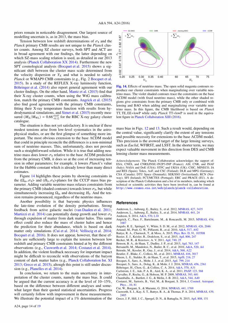
The situation is thus not yet satisfactory. It is unclear if thesemodest tensions arise from low-level systematics in the astro-physical studies, or are the first glimpse of something more im-portant. The most obvious extension to the base ΛCDM modelthat could in principle reconcile the differences is a non-minimalsum of neutrino masses. This, unfortunately, does not providesuch a straightforward solution. While it is true that adding neu-trino mass does lower σ8 relative to the base ΛCDM predictionfrom the primary CMB, it does so at the cost of increasing ten-sion in other parameters; for example, it lowers Planck’s valuefor the Hubble constant which is already lower than many directestimates.

Figure 14 highlights these points by showing constraints inthe (Ωm, σ8)- and (H0, σ8)-planes for the CCCP mass bias pa-rameter. Adding variable neutrino mass relaxes constraints fromthe primary CMB (shaded contours) towards lower σ8, but whilesimultaneously increasing Ωm and decreasing H0. And the ten-sion remains pronounced, regardless of the neutrino mass.

Another possibility is that baryonic physics influencesthe late-time evolution of the density perturbations. Strongfeedback from active galactic nuclei (van Daalen et al. 2011;Martizzi et al. 2014) can potentially damp growth and lower σ8through expulsion of matter from dark matter halos. This sameeffect could also reduce the mass of cluster halos and hencethe prediction for their abundance, which is based on darkmatter only simulations (Cui et al. 2014; Velliscig et al. 2014;Bocquet et al. 2016). It does not appear, however, that these ef-fects are sufficiently large to explain the tension between lowredshift and primary CMB constraints hinted at by the differentobservations (e.g., Cusworth et al. 2014; Costanzi et al. 2014).In addition, the violent feedback necessary for important impactmight be difficult to reconcile with observations of the baryoncontent of dark matter halos (e.g., Planck Collaboration Int. XI2013; Greco et al. 2015), altough this point is still under discus-sion (e.g., Planelles et al. 2014).

In conclusion, we return to the main uncertainty in inter-pretation of the cluster counts, namely the mass bias. It couldbe argued that the current accuracy is at the level of 10−15%,based on the difference between different analyses and some-what larger than their quoted statistical uncertainties. Progresswill certainly follow with improvement in these measurements.We illustrate the potential impact of a 1% determination of the

0.20 0.25 0.30 0.35 0.40Ωm

0.62

0.67

0.72

0.77

0.82

0.87

σ8

+∑

mν

SZ+BAO CMB +lensing+BAO ΛCDM

60 65 70 75H0

+∑

mν

Fig. 14. Effects of neutrino mass. The open solid magenta contours re-produce our cluster constraints when marginalizing over variable neu-trino mass. The violet shaded contours trace the constraints on the baseΛCDM model (with fixed neutrino mass), while the other shaded re-gions give constraints from the primary CMB only or combined withlensing and BAO when adding and marginalizing over variable neu-trino mass. In this figure, the CMB likelihood is based on PlanckTT, TE, EE+lowP while only Planck TT+lowP is used in the equiva-lent figure in Planck Collaboration XIII (2016).

mass bias in Figs. 12 and 13. Such a result would, depending onthe central value, significantly clarify the extent of any tensionsand possible necessity for extensions to the base ΛCDM model.This precision is the avowed target of the large lensing surveys,such as Euclid, WFIRST, and LSST. In the shorter term, we mayexpect valuable movement in this direction from DES and CMBlensing cluster mass measurements.

Acknowledgements. The Planck Collaboration acknowledges the support of:ESA; CNES, and CNRS/INSU-IN2P3-INP (France); ASI, CNR, and INAF(Italy); NASA and DoE (USA); STFC and UKSA (UK); CSIC, MINECO, JAand RES (Spain); Tekes, AoF, and CSC (Finland); DLR and MPG (Germany);CSA (Canada); DTU Space (Denmark); SER/SSO (Switzerland); RCN (Nor-way); SFI (Ireland); FCT/MCTES (Portugal); ERC and PRACE (EU). A de-scription of the Planck Collaboration and a list of its members, indicating whichtechnical or scientific activities they have been involved in, can be found athttp://www.cosmos.esa.int/web/planck/planck-collaboration.

ReferencesAnderson, L., Aubourg, E., Bailey, S., et al. 2012, MNRAS, 427, 3435Anderson, L., Aubourg, É., Bailey, S., et al. 2014, MNRAS, 441, 24Andreon, S. 2014, A&A, 570, L10Angrick, C., Pace, F., Bartelmann, M., & Roncarelli, M. 2015, MNRAS, 454,

1687Angulo, R. E., Springel, V., White, S. D. M., et al. 2012, MNRAS, 426, 2046Arnaud, M., Pratt, G. W., Piffaretti, R., et al. 2010, A&A, 517, A92Battye, R. A., Charnock, T., & Moss, A. 2015, Phys. Rev. D, 91, 103508Baxter, E. J., Keisler, R., Dodelson, S., et al. 2015, ApJ, 806, 247Becker, M. R., & Kravtsov, A. V. 2011, ApJ, 740, 25Benson, B. A., de Haan, T., Dudley, J. P., et al. 2013, ApJ, 763, 147Bersanelli, M., Mandolesi, N., Butler, R. C., et al. 2010, A&A, 520, A4Betoule, M., Kessler, R., Guy, J., et al. 2014, A&A, 568, A22Beutler, F., Blake, C., Colless, M., et al. 2011, MNRAS, 416, 3017Bleem, L. E., Stalder, B., de Haan, T., et al. 2015, ApJS, 216, 27Bocquet, S., Saro, A., Mohr, J. J., et al. 2015, ApJ, 799, 214Bocquet, S., Saro, A., Dolag, K., & Mohr, J. J. 2016, MNRAS, 456, 2361Böhringer, H., Chon, G., & Collins, C. A. 2014, A&A, 570, A31Carlstrom, J. E., Ade, P. A. R., Aird, K. A., et al. 2011, PASP, 123, 568Carvalho, P., Rocha, G., & Hobson, M. P. 2009, MNRAS, 393, 681Chamballu, A., Bartlett, J. G., & Melin, J.-B. 2012, A&A, 544, A40Costanzi, M., Sartoris, B., Viel, M., & Borgani, S. 2014, J. Cosmol. Astropart.

Phys. , 10, 81Cui, W., Borgani, S., & Murante, G. 2014, MNRAS, 441, 1769Cusworth, S. J., Kay, S. T., Battye, R. A., & Thomas, P. A. 2014, MNRAS, 439,

2485Greco, J. P., Hill, J. C., Spergel, D. N., & Battaglia, N. 2015, ApJ, 808, 151

A24, page 14 of 19

Planck Collaboration: Planck 2015 results. XXIV.

Hasselfield, M., Hilton, M., Marriage, T. A., et al. 2013, J. Cosmol. Astropart.Phys. , 7, 8

Hoekstra, H., Herbonnet, R., Muzzin, A., et al. 2015, MNRAS, 449, 685Hu, W., & Kravtsov, A. V. 2003, ApJ, 584, 702Lamarre, J., Puget, J., Ade, P. A. R., et al. 2010, A&A, 520, A9Lewis, A., & Challinor, A. 2006, Phys. Rep., 429, 1Madhavacheril, M., Sehgal, N., Allison, R., et al. 2015, Phys. Rev. Lett., 114,

151302Mantz, A. B., von der Linden, A., Allen, S. W., et al. 2015, MNRAS, 446, 2205Marrone, D. P., Smith, G. P., Okabe, N., et al. 2012, ApJ, 754, 119Martizzi, D., Mohammed, I., Teyssier, R., & Moore, B. 2014, MNRAS, 440,

2290Melin, J.-B., & Bartlett, J. G. 2015, A&A, 578, A21Melin, J., Bartlett, J. G., & Delabrouille, J. 2006, A&A, 459, 341Meneghetti, M., Rasia, E., Merten, J., et al. 2010, A&A, 514, A93Mennella, A., Butler, R. C., Curto, A., et al. 2011, A&A, 536, A3Merten, J., Meneghetti, M., Postman, M., et al. 2015, ApJ, 806, 4Nagai, D., Kravtsov, A. V., & Vikhlinin, A. 2007, ApJ, 668, 1Navarro, J. F., Frenk, C. S., & White, S. D. M. 1997, ApJ, 490, 493Olive, K. A. 2013, in AIP Conf. Ser., 1548, eds. L. A. Urenã-López, R. Becerril-

Bárcenas, & R. Linares-Romero, 116Padmanabhan, N., Xu, X., Eisenstein, D. J., et al. 2012, MNRAS, 427, 2132Piffaretti, R., & Valdarnini, R. 2008, A&A, 491, 71Piffaretti, R., Arnaud, M., Pratt, G. W., Pointecouteau, E., & Melin, J.-B. 2011,

A&A, 534, A109Planck Collaboration I. 2011, A&A, 536, A1Planck Collaboration I. 2014, A&A, 571, A1Planck Collaboration XVI. 2014, A&A, 571, A16Planck Collaboration XX. 2014, A&A, 571, A20Planck Collaboration XXIX. 2014, A&A, 571, A29Planck Collaboration I. 2016, A&A, 594, A1Planck Collaboration II. 2016, A&A, 594, A2Planck Collaboration III. 2016, A&A, 594, A3Planck Collaboration IV. 2016, A&A, 594, A4Planck Collaboration V. 2016, A&A, 594, A5Planck Collaboration VI. 2016, A&A, 594, A6Planck Collaboration VII. 2016, A&A, 594, A7Planck Collaboration VIII. 2016, A&A, 594, A8Planck Collaboration IX. 2016, A&A, 594, A9Planck Collaboration X. 2016, A&A, 594, A10Planck Collaboration XI. 2016, A&A, 594, A11Planck Collaboration XII. 2016, A&A, 594, A12Planck Collaboration XIII. 2016, A&A, 594, A13Planck Collaboration XIV. 2016, A&A, 594, A14Planck Collaboration XV. 2016, A&A, 594, A15Planck Collaboration XVI. 2016, A&A, 594, A16Planck Collaboration XVII. 2016, A&A, 594, A17Planck Collaboration XVIII. 2016, A&A, 594, A18Planck Collaboration XIX. 2016, A&A, 594, A19Planck Collaboration XX. 2016, A&A, 594, A20Planck Collaboration XXI. 2016, A&A, 594, A21Planck Collaboration XXII. 2016, A&A, 594, A22Planck Collaboration XXIII. 2016, A&A, 594, A23Planck Collaboration XXIV. 2016, A&A, 594, A24Planck Collaboration XXV. 2016, A&A, 594, A25Planck Collaboration XXVI. 2016, A&A, 594, A26Planck Collaboration XXVII. 2016, A&A, 594, A27Planck Collaboration XXVIII. 2016, A&A, 594, A28Planck Collaboration Int. III. 2013, A&A, 550, A129Planck Collaboration Int. XI. 2013, A&A, 557, A52Planck HFI Core Team 2011, A&A, 536, A4Planelles, S., Borgani, S., Fabjan, D., et al. 2014, MNRAS, 438, 195Postman, M., Coe, D., Benítez, N., et al. 2012, ApJS, 199, 25Rasia, E., Ettori, S., Moscardini, L., et al. 2006, MNRAS, 369, 2013Rasia, E., Meneghetti, M., Martino, R., et al. 2012, New J. Phys., 14, 055018Rasia, E., Lau, E. T., Borgani, S., et al. 2014, ApJ, 791, 96Reichardt, C. L., Stalder, B., Bleem, L. E., et al. 2013, ApJ, 763, 127Riess, A. G., Macri, L., Casertano, S., et al. 2011, ApJ, 730, 119Rozo, E., Bartlett, J. G., Evrard, A. E., & Rykoff, E. S. 2014a, MNRAS, 438, 78Rozo, E., Evrard, A. E., Rykoff, E. S., & Bartlett, J. G. 2014b, MNRAS, 438, 62Rozo, E., Rykoff, E. S., Bartlett, J. G., & Evrard, A. 2014c, MNRAS, 438, 49Simet, M., Battaglia, N., Mandelbaum, R., & Seljak, U. 2015, ArXiv e-prints

[arXiv:1502.01024]Steigman, G. 2008, ArXiv e-prints [arXiv:0807.3004]Swetz, D. S., Ade, P. A. R., Amiri, M., et al. 2011, ApJS, 194, 41Tauber, J. A., Mandolesi, N., Puget, J., et al. 2010, A&A, 520, A1Tinker, J., Kravtsov, A. V., Klypin, A., et al. 2008, ApJ, 688, 709Umetsu, K., Medezinski, E., Nonino, M., et al. 2014, ApJ, 795, 163

van Daalen, M. P., Schaye, J., Booth, C. M., & Dalla Vecchia, C. 2011, MNRAS,415, 3649

Velliscig, M., van Daalen, M. P., Schaye, J., et al. 2014, MNRAS, 442, 2641von der Linden, A., Allen, M. T., Applegate, D. E., et al. 2014a, MNRAS, 439,

2von der Linden, A., Mantz, A., Allen, S. W., et al. 2014b, MNRAS, 443, 1973Watson, W. A., Iliev, I. T., D’Aloisio, A., et al. 2013a, MNRAS, 433, 1230Watson, W. A., Iliev, I. T., D’Aloisio, A., et al. 2013b, MNRAS, submitted

[arXiv:1212.0095v1]Zaldarriaga, M., & Seljak, U. 1999, Phys. Rev. D, 59, 123507

1 APC, AstroParticule et Cosmologie, Université Paris Diderot,CNRS/IN2P3, CEA/lrfu, Observatoire de Paris, Sorbonne ParisCité, 10 rue Alice Domon et Léonie Duquet, 75205 Paris Cedex13, France

2 Aalto University Metsähovi Radio Observatory and Dept of RadioScience and Engineering, PO Box 13000, 00076 Aalto, Finland

3 African Institute for Mathematical Sciences, 6-8 Melrose Road,Muizenberg 7945, Cape Town, South Africa

4 Agenzia Spaziale Italiana Science Data Center, via del Politecnicosnc, 00133 Roma, Italy

5 Aix Marseille Université, CNRS, LAM (Laboratoired’Astrophysique de Marseille) UMR 7326, 13388 Marseille,France

6 Astrophysics Group, Cavendish Laboratory, University of Cam-bridge, J J Thomson Avenue, Cambridge CB3 0HE, UK

7 Astrophysics & Cosmology Research Unit, School of Mathemat-ics, Statistics & Computer Science, University of KwaZulu-Natal,Westville Campus, Private Bag X54001, 4000 South Africa

8 Atacama Large Millimeter/submillimeter Array, ALMA SantiagoCentral Offices, Alonso de Cordova 3107, Vitacura, 763 0355Casilla, Santiago, Chile

9 CGEE, SCS Qd 9, Lote C, Torre C, 4 andar, Ed. Parque CidadeCorporate, CEP 70308-200, Brasília, DF, Brazil

10 CITA, University of Toronto, 60 St. George St., Toronto, ON M5S3H8, Canada

11 CNRS, IRAP, 9 Av. colonel Roche, BP 44346, 31028 ToulouseCedex 4, France

12 CRANN, Trinity College, Dublin, Ireland13 California Institute of Technology, Pasadena, California,

CA 91125, USA14 Centre for Theoretical Cosmology, DAMTP, University of Cam-

bridge, Wilberforce Road, Cambridge CB3 0WA, UK15 Centro de Estudios de Física del Cosmos de Aragón (CEFCA),

Plaza San Juan 1, planta 2, 44001 Teruel, Spain16 Computational Cosmology Center, Lawrence Berkeley National

Laboratory, Berkeley, California, CA 94720, USA17 Consejo Superior de Investigaciones Científicas (CSIC), 28006

Madrid, Spain18 DSM/Irfu/SPP, CEA-Saclay, 91191 Gif-sur-Yvette Cedex, France19 DTU Space, National Space Institute, Technical University of

Denmark, Elektrovej 327, 2800 Kgs. Lyngby, Denmark20 Département de Physique Théorique, Université de Genève, 24

Quai E. Ansermet, 1211 Genève 4, Switzerland21 Departamento de Astrofísica, Universidad de La Laguna (ULL),

38206 La Laguna, Tenerife, Spain22 Departamento de Física, Universidad de Oviedo, Avda. Calvo

Sotelo s/n, 33007 Oviedo, Spain23 Department of Astronomy and Astrophysics, University of

Toronto, 50 Saint George Street, 38100 Toronto, Ontario, Canada24 Department of Astrophysics/IMAPP, Radboud University

Nijmegen, PO Box 9010, 6500 GL Nijmegen, The Netherlands25 Department of Physics & Astronomy, University of British

Columbia, 6224 Agricultural Road, Vancouver, British Columbia,Canada

26 Department of Physics and Astronomy, Dana and David DornsifeCollege of Letter, Arts and Sciences, University of SouthernCalifornia, Los Angeles, CA 90089, USA

27 Department of Physics and Astronomy, University CollegeLondon, London WC1E 6BT, UK

A24, page 15 of 19

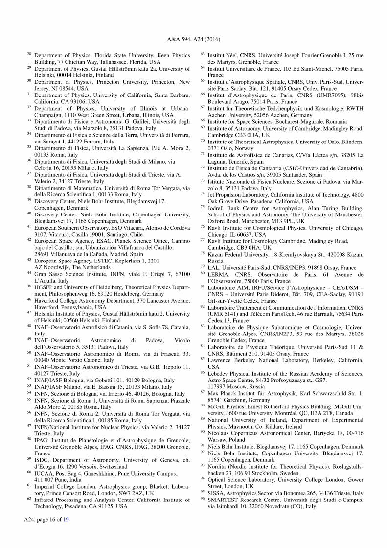
A&A 594, A24 (2016)

28 Department of Physics, Florida State University, Keen PhysicsBuilding, 77 Chieftan Way, Tallahassee, Florida, USA

29 Department of Physics, Gustaf Hällströmin katu 2a, University ofHelsinki, 00014 Helsinki, Finland

30 Department of Physics, Princeton University, Princeton, NewJersey, NJ 08544, USA

31 Department of Physics, University of California, Santa Barbara,California, CA 93106, USA

32 Department of Physics, University of Illinois at Urbana-Champaign, 1110 West Green Street, Urbana, Illinois, USA

33 Dipartimento di Fisica e Astronomia G. Galilei, Università degliStudi di Padova, via Marzolo 8, 35131 Padova, Italy

34 Dipartimento di Fisica e Scienze della Terra, Università di Ferrara,via Saragat 1, 44122 Ferrara, Italy

35 Dipartimento di Fisica, Università La Sapienza, P.le A. Moro 2,00133 Roma, Italy

36 Dipartimento di Fisica, Università degli Studi di Milano, viaCeloria 16, 20133 Milano, Italy

37 Dipartimento di Fisica, Università degli Studi di Trieste, via A.Valerio 2, 34127 Trieste, Italy

38 Dipartimento di Matematica, Università di Roma Tor Vergata, viadella Ricerca Scientifica 1, 00133 Roma, Italy

39 Discovery Center, Niels Bohr Institute, Blegdamsvej 17,Copenhagen, Denmark

40 Discovery Center, Niels Bohr Institute, Copenhagen University,Blegdamsvej 17, 1165 Copenhagen, Denmark

41 European Southern Observatory, ESO Vitacura, Alonso de Cordova3107, Vitacura, Casilla 19001, Santiago, Chile

42 European Space Agency, ESAC, Planck Science Office, Caminobajo del Castillo, s/n, Urbanización Villafranca del Castillo,28691 Villanueva de la Cañada, Madrid, Spain

43 European Space Agency, ESTEC, Keplerlaan 1, 2201AZ Noordwijk, The Netherlands

44 Gran Sasso Science Institute, INFN, viale F. Crispi 7, 67100L’Aquila, Italy

45 HGSFP and University of Heidelberg, Theoretical Physics Depart-ment, Philosophenweg 16, 69120 Heidelberg, Germany

46 Haverford College Astronomy Department, 370 Lancaster Avenue,Haverford, Pennsylvania, USA

47 Helsinki Institute of Physics, Gustaf Hällströmin katu 2, Universityof Helsinki, 00560 Helsinki, Finland

48 INAF–Osservatorio Astrofisico di Catania, via S. Sofia 78, Catania,Italy

49 INAF–Osservatorio Astronomico di Padova, Vicolodell’Osservatorio 5, 35131 Padova, Italy

50 INAF–Osservatorio Astronomico di Roma, via di Frascati 33,00040 Monte Porzio Catone, Italy

51 INAF–Osservatorio Astronomico di Trieste, via G.B. Tiepolo 11,40127 Trieste, Italy

52 INAF/IASF Bologna, via Gobetti 101, 40129 Bologna, Italy53 INAF/IASF Milano, via E. Bassini 15, 20133 Milano, Italy54 INFN, Sezione di Bologna, via Irnerio 46, 40126, Bologna, Italy55 INFN, Sezione di Roma 1, Università di Roma Sapienza, Piazzale

Aldo Moro 2, 00185 Roma, Italy56 INFN, Sezione di Roma 2, Università di Roma Tor Vergata, via

della Ricerca Scientifica 1, 00185 Roma, Italy57 INFN/National Institute for Nuclear Physics, via Valerio 2, 34127

Trieste, Italy58 IPAG: Institut de Planétologie et d’Astrophysique de Grenoble,

Université Grenoble Alpes, IPAG, CNRS, IPAG, 38000 Grenoble,France

59 ISDC, Department of Astronomy, University of Geneva, ch.d’Ecogia 16, 1290 Versoix, Switzerland

60 IUCAA, Post Bag 4, Ganeshkhind, Pune University Campus,411 007 Pune, India

61 Imperial College London, Astrophysics group, Blackett Labora-tory, Prince Consort Road, London, SW7 2AZ, UK

62 Infrared Processing and Analysis Center, California Institute ofTechnology, Pasadena, CA 91125, USA

63 Institut Néel, CNRS, Université Joseph Fourier Grenoble I, 25 ruedes Martyrs, Grenoble, France

64 Institut Universitaire de France, 103 Bd Saint-Michel, 75005 Paris,France

65 Institut d’Astrophysique Spatiale, CNRS, Univ. Paris-Sud, Univer-sité Paris-Saclay, Bât. 121, 91405 Orsay Cedex, France

66 Institut d’Astrophysique de Paris, CNRS (UMR7095), 98bisBoulevard Arago, 75014 Paris, France

67 Institut für Theoretische Teilchenphysik und Kosmologie, RWTHAachen University, 52056 Aachen, Germany

68 Institute for Space Sciences, Bucharest-Magurale, Romania69 Institute of Astronomy, University of Cambridge, Madingley Road,

Cambridge CB3 0HA, UK70 Institute of Theoretical Astrophysics, University of Oslo, Blindern,

0371 Oslo, Norway71 Instituto de Astrofísica de Canarias, C/Vía Láctea s/n, 38205 La

Laguna, Tenerife, Spain72 Instituto de Física de Cantabria (CSIC-Universidad de Cantabria),

Avda. de los Castros s/n, 39005 Santander, Spain73 Istituto Nazionale di Fisica Nucleare, Sezione di Padova, via Mar-

zolo 8, 35131 Padova, Italy74 Jet Propulsion Laboratory, California Institute of Technology, 4800

Oak Grove Drive, Pasadena, California, USA75 Jodrell Bank Centre for Astrophysics, Alan Turing Building,

School of Physics and Astronomy, The University of Manchester,Oxford Road, Manchester, M13 9PL, UK

76 Kavli Institute for Cosmological Physics, University of Chicago,Chicago, IL 60637, USA

77 Kavli Institute for Cosmology Cambridge, Madingley Road,Cambridge, CB3 0HA, UK

78 Kazan Federal University, 18 Kremlyovskaya St., 420008 Kazan,Russia

79 LAL, Université Paris-Sud, CNRS/IN2P3, 91898 Orsay, France80 LERMA, CNRS, Observatoire de Paris, 61 Avenue de

l’Observatoire, 75000 Paris, France81 Laboratoire AIM, IRFU/Service d’Astrophysique – CEA/DSM –

CNRS – Université Paris Diderot, Bât. 709, CEA-Saclay, 91191Gif-sur-Yvette Cedex, France

82 Laboratoire Traitement et Communication de l’Information, CNRS(UMR 5141) and Télécom ParisTech, 46 rue Barrault, 75634 ParisCedex 13, France

83 Laboratoire de Physique Subatomique et Cosmologie, Univer-sité Grenoble-Alpes, CNRS/IN2P3, 53 rue des Martyrs, 38026Grenoble Cedex, France

84 Laboratoire de Physique Théorique, Université Paris-Sud 11 &CNRS, Bâtiment 210, 91405 Orsay, France

85 Lawrence Berkeley National Laboratory, Berkeley, California,USA

86 Lebedev Physical Institute of the Russian Academy of Sciences,Astro Space Centre, 84/32 Profsoyuznaya st., GS7,117997 Moscow, Russia

87 Max-Planck-Institut für Astrophysik, Karl-Schwarzschild-Str. 1,85741 Garching, Germany

88 McGill Physics, Ernest Rutherford Physics Building, McGill Uni-versity, 3600 rue University, Montréal, QC, H3A 2T8, Canada

89 National University of Ireland, Department of ExperimentalPhysics, Maynooth, Co. Kildare, Ireland

90 Nicolaus Copernicus Astronomical Center, Bartycka 18, 00-716Warsaw, Poland

91 Niels Bohr Institute, Blegdamsvej 17, 1165 Copenhagen, Denmark92 Niels Bohr Institute, Copenhagen University, Blegdamsvej 17,

1165 Copenhagen, Denmark93 Nordita (Nordic Institute for Theoretical Physics), Roslagstulls-

backen 23, 106 91 Stockholm, Sweden94 Optical Science Laboratory, University College London, Gower

Street, London, UK95 SISSA, Astrophysics Sector, via Bonomea 265, 34136 Trieste, Italy96 SMARTEST Research Centre, Università degli Studi e-Campus,

via Isimbardi 10, 22060 Novedrate (CO), Italy

A24, page 16 of 19

Planck Collaboration: Planck 2015 results. XXIV.

97 School of Physics and Astronomy, Cardiff University, QueensBuildings, The Parade, Cardiff, CF24 3AA, UK

98 School of Physics and Astronomy, University of Nottingham,Nottingham NG7 2RD, UK

99 Sorbonne Université-UPMC, UMR7095, Institut d’Astrophysiquede Paris, 98bis Boulevard Arago, 75014, Paris, France

100 Space Research Institute (IKI), Russian Academy of Sciences,Profsoyuznaya Str, 84/32, 117997 Moscow, Russia

101 Space Sciences Laboratory, University of California, Berkeley,California, CA 94720, USA

102 Special Astrophysical Observatory, Russian Academy of Sci-ences, Nizhnij Arkhyz, Zelenchukskiy region, 369167 Karachai-Cherkessian Republic, Russia

103 Stanford University, Dept of Physics, Varian Physics Bldg,382 via Pueblo Mall, Stanford, California, CA 94305-4060, USA

104 Sub-Department of Astrophysics, University of Oxford, KebleRoad, Oxford OX1 3RH, UK

105 The Oskar Klein Centre for Cosmoparticle Physics, Department ofPhysics, Stockholm University, AlbaNova, 106 91 Stockholm,Sweden

106 Theory Division, PH-TH, CERN, 1211 Geneva 23, Switzerland107 UPMC Univ. Paris 06, UMR7095, 98bis Boulevard Arago,

75014 Paris, France108 Université de Toulouse, UPS-OMP, IRAP, 31028 Toulouse Cedex

4, France109 University Observatory, Ludwig Maximilian University of Munich,

Scheinerstrasse 1, 81679 Munich, Germany110 University of Granada, Departamento de Física Teórica y del Cos-

mos, Facultad de Ciencias, 81679 Granada, Spain111 University of Granada, Instituto Carlos I de Física Teórica y Com-

putacional, Granada, Spain112 Warsaw University Observatory, Aleje Ujazdowskie 4,

00-478 Warszawa, Poland

A24, page 17 of 19

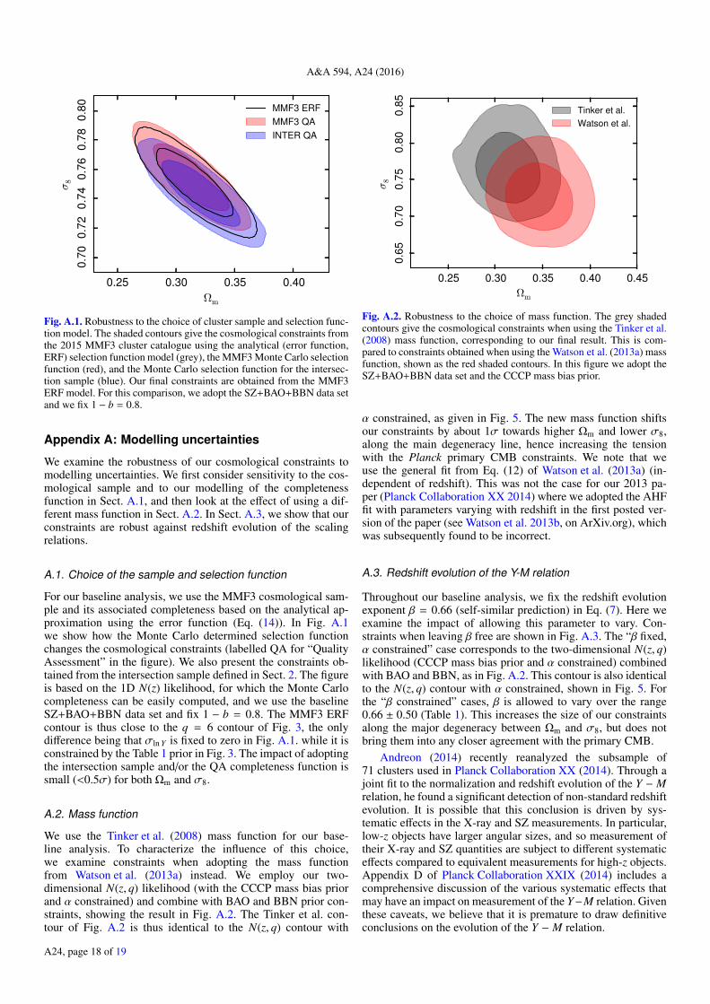
A&A 594, A24 (2016)

0.25 0.30 0.35 0.40Ωm

0.70

0.72

0.74

0.76

0.78

0.80

σ8

MMF3 ERFMMF3 QAINTER QA

Fig. A.1. Robustness to the choice of cluster sample and selection func-tion model. The shaded contours give the cosmological constraints fromthe 2015 MMF3 cluster catalogue using the analytical (error function,ERF) selection function model (grey), the MMF3 Monte Carlo selectionfunction (red), and the Monte Carlo selection function for the intersec-tion sample (blue). Our final constraints are obtained from the MMF3ERF model. For this comparison, we adopt the SZ+BAO+BBN data setand we fix 1 − b = 0.8.

Appendix A: Modelling uncertainties

We examine the robustness of our cosmological constraints tomodelling uncertainties. We first consider sensitivity to the cos-mological sample and to our modelling of the completenessfunction in Sect. A.1, and then look at the effect of using a dif-ferent mass function in Sect. A.2. In Sect. A.3, we show that ourconstraints are robust against redshift evolution of the scalingrelations.

A.1. Choice of the sample and selection function

For our baseline analysis, we use the MMF3 cosmological sam-ple and its associated completeness based on the analytical ap-proximation using the error function (Eq. (14)). In Fig. A.1we show how the Monte Carlo determined selection functionchanges the cosmological constraints (labelled QA for “QualityAssessment” in the figure). We also present the constraints ob-tained from the intersection sample defined in Sect. 2. The figureis based on the 1D N(z) likelihood, for which the Monte Carlocompleteness can be easily computed, and we use the baselineSZ+BAO+BBN data set and fix 1 − b = 0.8. The MMF3 ERFcontour is thus close to the q = 6 contour of Fig. 3, the onlydifference being that σln Y is fixed to zero in Fig. A.1. while it isconstrained by the Table 1 prior in Fig. 3. The impact of adoptingthe intersection sample and/or the QA completeness function issmall (<0.5σ) for both Ωm and σ8.

A.2. Mass function

We use the Tinker et al. (2008) mass function for our base-line analysis. To characterize the influence of this choice,we examine constraints when adopting the mass functionfrom Watson et al. (2013a) instead. We employ our two-dimensional N(z, q) likelihood (with the CCCP mass bias priorand α constrained) and combine with BAO and BBN prior con-straints, showing the result in Fig. A.2. The Tinker et al. con-tour of Fig. A.2 is thus identical to the N(z, q) contour with

0.25 0.30 0.35 0.40 0.45Ωm

0.65

0.70

0.75

0.80

0.85

σ8

Tinker et al.Watson et al.

Fig. A.2. Robustness to the choice of mass function. The grey shadedcontours give the cosmological constraints when using the Tinker et al.(2008) mass function, corresponding to our final result. This is com-pared to constraints obtained when using the Watson et al. (2013a) massfunction, shown as the red shaded contours. In this figure we adopt theSZ+BAO+BBN data set and the CCCP mass bias prior.

α constrained, as given in Fig. 5. The new mass function shiftsour constraints by about 1σ towards higher Ωm and lower σ8,along the main degeneracy line, hence increasing the tensionwith the Planck primary CMB constraints. We note that weuse the general fit from Eq. (12) of Watson et al. (2013a) (in-dependent of redshift). This was not the case for our 2013 pa-per (Planck Collaboration XX 2014) where we adopted the AHFfit with parameters varying with redshift in the first posted ver-sion of the paper (see Watson et al. 2013b, on ArXiv.org), whichwas subsequently found to be incorrect.

A.3. Redshift evolution of the Y-M relation

Throughout our baseline analysis, we fix the redshift evolutionexponent β = 0.66 (self-similar prediction) in Eq. (7). Here weexamine the impact of allowing this parameter to vary. Con-straints when leaving β free are shown in Fig. A.3. The “β fixed,α constrained” case corresponds to the two-dimensional N(z, q)likelihood (CCCP mass bias prior and α constrained) combinedwith BAO and BBN, as in Fig. A.2. This contour is also identicalto the N(z, q) contour with α constrained, shown in Fig. 5. Forthe “β constrained” cases, β is allowed to vary over the range0.66 ± 0.50 (Table 1). This increases the size of our constraintsalong the major degeneracy between Ωm and σ8, but does notbring them into any closer agreement with the primary CMB.

Andreon (2014) recently reanalyzed the subsample of71 clusters used in Planck Collaboration XX (2014). Through ajoint fit to the normalization and redshift evolution of the Y − Mrelation, he found a significant detection of non-standard redshiftevolution. It is possible that this conclusion is driven by sys-tematic effects in the X-ray and SZ measurements. In particular,low-z objects have larger angular sizes, and so measurement oftheir X-ray and SZ quantities are subject to different systematiceffects compared to equivalent measurements for high-z objects.Appendix D of Planck Collaboration XXIX (2014) includes acomprehensive discussion of the various systematic effects thatmay have an impact on measurement of the Y−M relation. Giventhese caveats, we believe that it is premature to draw definitiveconclusions on the evolution of the Y − M relation.

A24, page 18 of 19

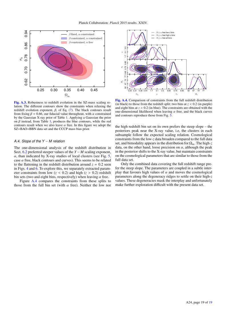
Planck Collaboration: Planck 2015 results. XXIV.

0.25 0.30 0.35 0.40 0.45Ωm

0.62

0.70

0.78

0.86

0.94

σ8

β fixed, α constrained

β constrained, α constrained

β constrained, α free

Fig. A.3. Robustness to redshift evolution in the SZ-mass scaling re-lation. The different contours show the constraints when relaxing theredshift evolution exponent, β, of Eq. (7). The black contours resultfrom fixing β = 0.66, our fiducial value throughout, with α constrainedby the Gaussian X-ray prior of Table 1. Applying a Gaussian the prioron β instead, from Table 1, produces the blue contours, while the redcontours result when we also leave α free. In this figure we adopt theSZ+BAO+BBN data set and the CCCP mass bias prior.

A.4. Slope of the Y −M relation

The one-dimensional analysis of the redshift distribution inSect. 6.2 preferred steeper values of the Y −M scaling exponent,α, than indicated by X-ray studies of local clusters (see Fig. 5,case α free, black contours and curves). This seems to be relatedto the flattening in the redshift distribution around z = 0.2 seenin Figs. 4 and 6. To explore this, we separately extracted param-eter constraints from low (z < 0.2) and high (z > 0.2) redshiftbin sets (two and eight bins, respectively) when leaving α free.

Figure A.4 compares the constraints from these splits tothose from the full bin set (with α free). Neither the low nor

0.25 0.31 0.38 0.44

N(z) α free low-z binsN(z) α free high-z binsN(z) α free all bins

0.25 0.31 0.38 0.44

1.7

2.1

2.5

α

1.7 2.1 2.5

0.25 0.31 0.38 0.44

0.65

0.75

0.85

σ8

1.7 2.1 2.5 0.65 0.75 0.85

0.25 0.31 0.38 0.44Ωm

6267

7277

H0

1.7 2.1 2.5α

0.65 0.75 0.85σ8

62 67 72 77H0

Fig. A.4. Comparison of constraints from the full redshift distribution(in black) to those from the redshift split: two bins at z < 0.2 (in purple)and eight bins at z > 0.2 (in blue). The constraints are obtained with theone-dimensional likelihood when leaving α free, and the black curvesand contours reproduce those from Fig. 5.

the high redshift bin set on its own prefers the steep slope – theposteriors peak near the X-ray value, i.e, the clusters in eachsubsample follow the expected scaling relation. Cosmologicalconstraints from the low-z data broaden compared to the full dataset, and bimodality appears in the distribution for Ωm. The high-zdata, on the other hand, loose precision on α, although the peakin the posterior shifts to the X-ray value, but maintain constraintson the cosmological parameters that are similar to those from thefull data set.

Only the combined data covering the full redshift range pre-fer the steep slope. The parameters are coupled in a subtle inter-play that favours high values of α and moves the cosmologicalparameters along the degeneracy ridges to settle on their high-zvalues. These degeneracies mask the interplay and unfortunatelymake further exploration difficult with the present data set.

A24, page 19 of 19