A&A 594, A23 (2016)DOI: 10.1051/0004-6361/201527418c© ESO 2016

Astronomy&Astrophysics

Planck 2015 results Special feature

Planck 2015 results

XXIII. The thermal Sunyaev-Zeldovich effect-cosmic infrared backgroundcorrelation

Planck Collaboration: P. A. R. Ade82, N. Aghanim57, M. Arnaud71, J. Aumont57, C. Baccigalupi81, A. J. Banday89, 9, R. B. Barreiro62,J. G. Bartlett1, 64, N. Bartolo27, 63, E. Battaner90, 91, K. Benabed58, 88, A. Benoit-Lévy21, 58, 88, J.-P. Bernard89, 9, M. Bersanelli30, 47, P. Bielewicz78, 9, 81,

J. J. Bock64, 10, A. Bonaldi65, L. Bonavera62, J. R. Bond8, J. Borrill12, 85, F. R. Bouchet58, 83, C. Burigana46, 28, 48, R. C. Butler46, E. Calabrese87,A. Catalano72, 70, A. Chamballu71, 13, 57, H. C. Chiang24, 6, P. R. Christensen79, 33, E. Churazov76, 84, D. L. Clements54, L. P. L. Colombo20, 64,

C. Combet72, B. Comis72, F. Couchot69, A. Coulais70, B. P. Crill64, 10, A. Curto62, 5, 67, F. Cuttaia46, L. Danese81, R. D. Davies65, R. J. Davis65,P. de Bernardis29, A. de Rosa46, G. de Zotti43, 81, J. Delabrouille1, C. Dickinson65, J. M. Diego62, H. Dole57, 56, S. Donzelli47, O. Doré64, 10,

M. Douspis57, A. Ducout58, 54, X. Dupac35, G. Efstathiou59, F. Elsner21, 58, 88, T. A. Enßlin76, H. K. Eriksen60, F. Finelli46, 48, I. Flores-Cacho9, 89,O. Forni89, 9, M. Frailis45, A. A. Fraisse24, E. Franceschi46, S. Galeotta45, S. Galli66, K. Ganga1, R. T. Génova-Santos61, 16, M. Giard89, 9,Y. Giraud-Héraud1, E. Gjerløw60, J. González-Nuevo17, 62, K. M. Górski64, 92, A. Gregorio31, 45, 51, A. Gruppuso46, J. E. Gudmundsson24,

F. K. Hansen60, D. L. Harrison59, 67, G. Helou10, C. Hernández-Monteagudo11, 76, D. Herranz62, S. R. Hildebrandt64, 10, E. Hivon58, 88, M. Hobson5,A. Hornstrup14, W. Hovest76, K. M. Huffenberger22, G. Hurier57,?, A. H. Jaffe54, T. R. Jaffe89, 9, W. C. Jones24, E. Keihänen23, R. Keskitalo12,

T. S. Kisner74, R. Kneissl34, 7, J. Knoche76, M. Kunz15, 57, 2, H. Kurki-Suonio23, 41, G. Lagache4, 57, J.-M. Lamarre70, M. Langer57, A. Lasenby5, 67,M. Lattanzi28, C. R. Lawrence64, R. Leonardi35, F. Levrier70, P. B. Lilje60, M. Linden-Vørnle14, M. López-Caniego35, 62, P. M. Lubin25,

J. F. Macías-Pérez72, B. Maffei65, G. Maggio45, D. Maino30, 47, D. S. Y. Mak59, 67, N. Mandolesi46, 28, A. Mangilli57, 69, M. Maris45, P. G. Martin8,E. Martínez-González62, S. Masi29, S. Matarrese27, 63, 38, A. Melchiorri29, 49, A. Mennella30, 47, M. Migliaccio59, 67, S. Mitra53, 64,

M.-A. Miville-Deschênes57, 8, A. Moneti58, L. Montier89, 9, G. Morgante46, D. Mortlock54, D. Munshi82, J. A. Murphy77, F. Nati24, P. Natoli28, 3, 46,F. Noviello65, D. Novikov75, I. Novikov79, 75, C. A. Oxborrow14, F. Paci81, L. Pagano29, 49, F. Pajot57, D. Paoletti46, 48, B. Partridge40, F. Pasian45,T. J. Pearson10, 55, O. Perdereau69, L. Perotto72, V. Pettorino39, F. Piacentini29, M. Piat1, E. Pierpaoli20, S. Plaszczynski69, E. Pointecouteau89, 9,

G. Polenta3, 44, N. Ponthieu57, 52, G. W. Pratt71, S. Prunet58, 88, J.-L. Puget57, J. P. Rachen18, 76, M. Reinecke76, M. Remazeilles65, 57, 1, C. Renault72,A. Renzi32, 50, I. Ristorcelli89, 9, G. Rocha64, 10, C. Rosset1, M. Rossetti30, 47, G. Roudier1, 70, 64, J. A. Rubiño-Martín61, 16, B. Rusholme55,

M. Sandri46, D. Santos72, M. Savelainen23, 41, G. Savini80, D. Scott19, L. D. Spencer82, V. Stolyarov5, 86, 68, R. Stompor1, R. Sunyaev76, 84,D. Sutton59, 67, A.-S. Suur-Uski23, 41, J.-F. Sygnet58, J. A. Tauber36, L. Terenzi37, 46, L. Toffolatti17, 62, 46, M. Tomasi30, 47, M. Tristram69, M. Tucci15,

G. Umana42, L. Valenziano46, J. Valiviita23, 41, B. Van Tent73, P. Vielva62, F. Villa46, L. A. Wade64, B. D. Wandelt58, 88, 26, I. K. Wehus64,N. Welikala87, D. Yvon13, A. Zacchei45, and A. Zonca25

(Affiliations can be found after the references)

Received 22 September 2015 / Accepted 23 April 2016

ABSTRACT

We use Planck data to detect the cross-correlation between the thermal Sunyaev-Zeldovich (tSZ) effect and the infrared emission from the galaxiesthat make up the the cosmic infrared background (CIB). We first perform a stacking analysis towards Planck-confirmed galaxy clusters. We detectinfrared emission produced by dusty galaxies inside these clusters and demonstrate that the infrared emission is about 50% more extended than thetSZ effect. Modelling the emission with a Navarro-Frenk-White profile, we find that the radial profile concentration parameter is c500 = 1.00+0.18

−0.15.This indicates that infrared galaxies in the outskirts of clusters have higher infrared flux than cluster-core galaxies. We also study the cross-correlation between tSZ and CIB anisotropies, following three alternative approaches based on power spectrum analyses: (i) using a catalogue ofconfirmed clusters detected in Planck data; (ii) using an all-sky tSZ map built from Planck frequency maps; and (iii) using cross-spectra betweenPlanck frequency maps. With the three different methods, we detect the tSZ-CIB cross-power spectrum at significance levels of (i) 6σ; (ii) 3σ; and(iii) 4σ. We model the tSZ-CIB cross-correlation signature and compare predictions with the measurements. The amplitude of the cross-correlationrelative to the fiducial model is AtSZ−CIB = 1.2±0.3. This result is consistent with predictions for the tSZ-CIB cross-correlation assuming the best-fitcosmological model from Planck 2015 results along with the tSZ and CIB scaling relations.

Key words. galaxies: clusters: general – infrared: galaxies – large-scale structure of Universe – methods: data analysis

? Corresponding author: Guillaume Hurier, e-mail: ghurier@ias.u-psud.fr

Article published by EDP Sciences A23, page 1 of 17

A&A 594, A23 (2016)

1. Introduction

This paper is one of a set associated with the 2015 release ofdata from the Planck1 mission. It reports the first all-sky de-tection of the cross-correlation between the thermal Sunyaev-Zeldovich (tSZ) effect (Sunyaev & Zeldovich 1969, 1972) andthe cosmic infrared background (CIB; Puget et al. 1996; Fixsenet al. 1998; Hauser et al. 1998). An increasing number of ob-servational studies are measuring the tSZ effect and CIB fluctua-tions at infrared and submillimetre wavelengths, including inves-tigations of the CIB with the Spitzer Space Telescope (Lagacheet al. 2007) and the Herschel Space Observatory (Amblard et al.2011; Viero et al. 2012, 2015), and observations of the tSZ effectwith instruments such as the Atacama Pathfinder Experiment(Halverson et al. 2009) and Bolocam (Sayers et al. 2011). Inaddition, a new generation of CMB experiments can measurethe tSZ effect and CIB at microwave frequencies (Hincks et al.2010; Hall et al. 2010; Dunkley et al. 2011; Zwart et al. 2011;Reichardt et al. 2012; Planck Collaboration XXI 2014; PlanckCollaboration XXX 2014).

The large frequency coverage of Planck, from 30to 857 GHz, makes it sensitive to both of these important probesof large-scale structure. At intermediate frequencies, from 70to 217 GHz, the sky emission is dominated by the cosmic mi-crowave background (CMB). At these frequencies, it is pos-sible to detect galaxy clusters that produce a distortion of theCMB blackbody emission through the tSZ effect. At the angu-lar resolution of Planck, this effect is mainly produced by lo-cal (z < 1) and massive galaxy clusters in dark matter halos(above 1014 M), and it has been used for several studies ofcluster physics and cosmology (e.g., Planck Collaboration X2011; Planck Collaboration XI 2011; Planck Collaboration Int.III 2013; Planck Collaboration Int. V 2013; Planck CollaborationInt. VIII 2013; Planck Collaboration Int. X 2013; PlanckCollaboration XX 2014; Planck Collaboration XXIV 2016;Planck Collaboration XX 2014; Planck Collaboration XXIV2016). At frequencies above 353 GHz, the sky emission isdominated by thermal emission, both Galactic and extragalac-tic (Planck Collaboration XI 2014; Planck Collaboration XXX2014). The dominant extragalactic signal is the thermal infraredemission from dust heated by UV radiation from young stars.According to our current knowledge of star-formation history,the CIB emission has a peak in its redshift distribution betweenz = 1 and z = 2, and is produced by galaxies in dark matter halosof 1011–1013 M; this has been confirmed through the measuredstrong correlation between the CIB and CMB lensing (PlanckCollaboration XVIII 2014). However, owing to the different red-shift and mass ranges, the CIB and tSZ distributions have littleoverlap at the angular scales probed by Planck, making this cor-relation hard to detect.

Nevertheless, determining the strength of this tSZ-CIB cor-relation is important for several reasons. Certainly we needto know the extent to which tSZ estimates might be contam-inated by CIB fluctuations, but uncertainty in the correlationalso degrades our ability to estimate power coming from the ki-netic SZ effect (arising from peculiar motions), which promisesto probe the reionization epoch (e.g., Mesinger et al. 2012;

1 Planck (http://www.esa.int/Planck) is a project of theEuropean Space Agency (ESA) with instruments provided by two sci-entific consortia funded by ESA member states and led by PrincipalInvestigators from France and Italy, telescope reflectors providedthrough a collaboration between ESA and a scientific consortium ledand funded by Denmark, and additional contributions from NASA(USA).

Reichardt et al. 2012; Planck Collaboration Int. XXXVII 2016).But, as well as this analysis of the tSZ-CIB correlation enablesus to better understand the spatial distribution and evolution ofstar formation within massive halos.

The profile of infrared emission from galaxy clusters is ex-pected to be less concentrated than the profile of the numbercounts of galaxies. Indeed, core galaxies present reduced in-frared emission owing to quenching, which occurs after theymake their first passage inside r ' R500 (Muzzin et al. 2014).Using SDSS data, Weinmann et al. (2010) computed the ra-dial profile of passive galaxies for high-mass galaxy clusters(M > 1014 M). They found that the fraction of passive galaxiesis 70–80% at the centres and 25–35% in the outskirts of clusters.The detection of infrared emission cluster by cluster is difficult atmillimetre wavelengths, since the emission is faint and confusedby the fluctuations of the infrared sky (Galactic thermal dust andCIB). Statistical detections of infrared emission in galaxy clus-ters have been made by stacking large samples of known clusters(Montier & Giard 2005; Giard et al. 2008; Roncarelli et al. 2010)in IRAS data (Wheelock et al. 1993). The stacking approachhas also been shown to be a powerful method for extracting thetSZ signal from microwave data (e.g., Lieu et al. 2006; Diego &Partridge 2009).

Recently, efforts have been made to model the tSZ-CIB cor-relation (e.g., Zahn et al. 2012; Addison et al. 2012). Usinga halo model, it is possible to predict the tSZ-CIB cross-correlation. The halo model approach enables us to consider dis-tinct astrophysical emission processes that trace the large-scaledark matter density fluctuation, but have different dependencieson the host halo mass and redshift. In this paper, we use mod-els of the tSZ-CIB cross-correlation at galaxy cluster scales. Wenote that the tSZ effect does not possess significant substructureon the scale of galaxies, so the tSZ-CIB cross-correlation shouldnot possess a shot noise term.

Current experiments have already provided constraints onthe tSZ-CIB cross-correlation at low frequencies, between 100and 250 GHz. The ACT collaboration sets an upper limit ρ < 0.2on the tSZ-CIB cross correlation (Dunkley et al. 2013). Georgeet al. (2015), using SPT data and assuming a single correlationfactor, obtained a tSZ-CIB correlation factor of 0.11+0.06

−0.05; a zerocorrelation is disfavoured at a confidence level of 99%.

Our objective in this paper is twofold. First, we characterizethe CIB emission toward tSZ-detected galaxy clusters by con-straining the profile and redshift dependence of CIB emissionfrom galaxy clusters. Then, we set constraints on the overall tSZ-CIB cross-correlation power spectrum, and report the first all-sky detection of the tSZ-CIB angular cross-power spectra, at asignificance level of 4σ. Our models and results on the tSZ-CIBcross-correlation have been used in a companion Planck paperPlanck Collaboration XXII (2016).

In the first part of Sect. 2, we explain our modelling approachfor the tSZ effect and CIB emission at the galaxy cluster scale.In the second part of Sect. 2, we describe the model for the tSZ,CIB, and tSZ-CIB power and cross-power spectra using a halomodel. Then in Sect. 3 we present the data sets we have used.Sections 4 and 5 present our results for the SED, shape, andcross-spectrum of the tSZ-CIB correlation. Finally, in Sect. 6 wediscuss the results and their consistency with previous analyses.

Throughout this paper, the tSZ effect intensity is expressedin units of Compton parameter, and we use the best-fit cosmol-ogy from Planck Collaboration XIII (2016, fourth column ofTable 3) using “TT, TE, EE+lowP” values as the fiducial cos-mological model, unless otherwise specified. Thus, we adoptH0 = 67.27 km s−1 Mpc1, σ8 = 0.831, and Ωm = 0.3156.

A23, page 2 of 17

Planck Collaboration: Planck 2015 results. XXIII.

Table 1. Cosmological and scaling-law parameters for our fiducialmodel, for both the Y500–M500 relation (Planck Collaboration XX2014) and the L500–M500 relation (fitted to spectra from PlanckCollaboration XXX 2014).

Planck-SZ cosmologyΩm . . . . . . . . 0.29 ± 0.02σ8 . . . . . . . . . 0.77 ± 0.02H0 . . . . . . . . 67.3 ± 1.4

Planck-CMB cosmologyΩm . . . . . . . . 0.316 ± 0.009σ8 . . . . . . . . . 0.831 ± 0.013H0 . . . . . . . . 67.27 ± 0.66

M500–Y500log Y∗ . . . . . . −0.19 ± 0.02αSZ . . . . . . . . 1.79 ± 0.08βSZ . . . . . . . . 0.66 ± 0.50

M500–L500Td0 . . . . . . . . 24.4 ± 1.9αCIB . . . . . . . 0.36 ± 0.05βCIB . . . . . . . 1.75 ± 0.06γCIB . . . . . . . 1.70 ± 0.02δCIB . . . . . . . . 3.2 ± 0.2εCIB . . . . . . . . 1.0

2. Modelling

To model the cross-correlation between tSZ and CIBanisotropies we have to relate the mass, M500, and the redshift, z,of a given cluster to tSZ flux, Y500, and CIB luminosity L500.We define M500 (and R500) as the total mass (and radius) forwhich the mean over-density is 500 times the critical density ofthe Universe. Considering that the tSZ signal in the Planck datahas no significant substructure at galaxy scales, we modelled thetSZ-CIB cross-correlation at the galaxy cluster scale. This can beconsidered as a large-scale approximation for the CIB emission,and at the Planck angular resolution it agrees with the more re-fined modelling presented in Planck Collaboration XXX (2014).

2.1. The thermal Sunyaev-Zeldovich effect

The tSZ effect is a small-amplitude distortion of the CMB black-body spectrum caused by inverse-Compton scattering (see, e.g.,Rephaeli 1995; Birkinshaw 1999; Carlstrom et al. 2002). Its in-tensity is related to the integral of the pressure along the line ofsight via the Compton parameter, which for a given direction onthe sky is

y =

∫kBσT

mec2 neTedl. (1)

Here dl is the distance along the line of sight, kB, σT, me, and care the usual physical constants, and ne and Te are the electronnumber density and the temperature, respectively.

In units of CMB temperature, the contribution of the tSZ ef-fect to the submillimetre sky intensity for a given observationfrequency ν is given by

∆TCMB

TCMB= g(ν)y. (2)

Neglecting relativistic corrections we have g(ν) = x coth(x/2) −4, with x = hν/(kBTCMB). The function g(ν) is is equal to 0 at

about 217 GHz, and is negative at lower frequencies and positiveat higher frequencies.

We have used the M500–Y500 scaling law presented in PlanckCollaboration XX (2014),

E−βSZ (z) D2

A(z)Y500

10−4 Mpc2

= Y∗

[h

0.7

]−2+αSZ[

(1 − b)M500

6 × 1014 M

]αSZ

, (3)

with E(z) =√

Ωm(1 + z)3 + ΩΛ for a flat universe. The coeffi-cients Y∗, αSZ, and βSZ are taken from Planck Collaboration XX(2014), and are given in Table 1. The mean bias, (1−b), betweenX-ray mass and the true mass is discussed in detail in PlanckCollaboration XX (2014, Appendix A) and references therein.We adopt b = 0.3 here, which, given the chosen cosmologicalparameters, enables us to reproduce the tSZ results from PlanckCollaboration XXII (2016) and Planck Collaboration XXIV(2016).

2.2. Cosmic infrared background emission

The CIB is the diffuse emission from galaxies integratedthroughout cosmic history (see, e.g., Hauser & Dwek 2001;Lagache et al. 2005), and is thus strongly related to the star-formation rate history. The CIB intensity, I(ν), at frequency νcan be written as

I(ν) =

∫dz

dχ(z)dz

j(ν, z)(1 + z)

, (4)

with χ(z) the comoving distance and j(ν, z) the emissivity that isrelated to the star-formation density, ρSFR, through

j(ν, z) =ρSFR(z)(1 + z)Θeff(ν, z)χ2(z)

K, (5)

where K is the Kennicutt (1998) constant (SFR/LIR = 1.7 ×10−10 M yr−1) and Θeff(ν, z) the mean spectral energy distribu-tion (SED) of infrared galaxies at redshift z.

To model the L500–M500 relation we use a parametric relationproposed by Shang et al. (2012) that relates the CIB flux, L500,to the mass, M500, as follows:

L500(ν) = L0

[M500

1 × 1014 M

]εCIB

Ψ(z) Θ [(1 + z)ν,Td(z)] , (6)

where L0 is a normalization parameter, Td(z) = Td0(1 + z)αCIB

and Θ [ν,Td] is the typical SED of a galaxy that contributes tothe total CIB emission,

Θ [ν,Td] =

ν βCIB Bν(Td), if ν < ν0,ν−γCIB , if ν ≥ ν0,

with ν0 being the solution of dlog[ν βCIB Bν(Td)]/dlog(ν) = −γCIB.We assume a redshift dependence of the form

Ψ(z) = (1 + z)δCIB . (7)

We also define S 500 as

S 500(ν) =L500(ν)

4π(1 + z)χ2(z)· (8)

The coefficients Td0, αCIB, βCIB, γCIB, and δCIB from PlanckCollaboration XXX (2014) are given in Table 1. We fix the valueof εCIB to 1. In Sect. 2.5, this model of the CIB emission is com-pared with the Planck measurement of the CIB power spectra.We stress that this parametrization can only be considered accu-rate at scales where galaxy clusters are not (or only marginally)extended. This is typically the case at Planck angular resolutionfor the low-mass and high-redshift dark matter halos that domi-nate the total CIB emission.

A23, page 3 of 17

A&A 594, A23 (2016)

2.3. Angular power spectra

2.3.1. The halo model

To model tSZ, CIB, and tSZ-CIB angular power spectra, we con-sider the halo-model formalism (see, e.g., Cooray & Sheth 2002)and the following general expression

C` = CAB,1h`

+ CAB,2h`

, (9)

where A and B stand for tSZ effect or CIB emission, CAB,1h`

is the1-halo contribution, and CAB,2h

`is the 2-halo term that accounts

for correlation in the spatial distribution of halos over the sky.The 1-halo term CAB,1h

`is computed using the Fourier trans-

form of the projected profiles of signals A and B weighted by themass function and the A and B emission (see, e.g., Komatsu &Seljak 2002, for a derivation of the tSZ angular power spectrum):

CAB,1h`

= 4π∫

dzdV

dzdΩ

∫dM

d2NdMdV

WA,1hWB,1h, (10)

where d2N/dMdV is the dark-matter halo mass function fromTinker et al. (2008), dV/dzdΩ is the comoving volume element,and WA,1h, WB,1h are the window functions that account for se-lection effects and total halo signal. For the tSZ effect, we haveW1h

tSZ = WN(Y500)Y500y`(M500, z) and WN(Y500) is a weight, rang-ing from 0 to 1, applied to the mass function to account for theeffective number of clusters used in our analysis; here Y500 is thetSZ flux, and y` is the Fourier transform of the tSZ profile. Forthe CIB emission we have W1h

CIB = S 500(ν)I`(M500, z), where I`the Fourier transform of the infrared profile (from Eq. (18)) andS 500(ν) is given in Eq. (8).

The results for the radial analysis in Sect. 4.1.3 show thatthe infrared emission profile can be well approximated by anNFW profile (Navarro et al. 1997) with a concentration parame-ter c500 = 1.0. The galaxy cluster pressure profile is modelled bya generalized NFW profile (GNFW, Nagai et al. 2007) using thebest-fit values from Arnaud et al. (2010).

The contribution of the 2-halo term, CAB,2h`

, accounts forlarge-scale fluctuations in the matter power spectrum that inducecorrelations in the dark-matter halo distribution over the sky. Itcan be computed as

CAB,2h`

= 4π∫

dzdV

dzdΩ

(∫dM

d2NdMdV

WA,1hblin(M, z))

×

(∫dM

d2NdMdV

WB,1hblin(M, z))

P(k, z) (11)

(see, e.g., Taburet et al. 2011, and references therein), whereP(k, z) is the matter power spectrum computed using CLASS(Lesgourgues 2011) and blin(M, z) is the time-dependent linearbias factor (see Mo & White 1996; Komatsu & Kitayama 1999;Tinker et al. 2010, for an analytical formula).

As already stated, at the Planck resolution the tSZ emis-sion does not have substructures at galaxy scales. Consequentlythere is no shot-noise in the tSZ auto-spectrum and all the tSZ-related cross-spectra. Considering the method we used to com-pute the CIB auto-correlation power spectra, the total amplitudeof the 1-halo term should include this “shot-noise” (galaxy auto-correlation). We have verified that, at the resolution of Planck,there is no significant difference between our modelling and a di-rect computation of the shot-noise using the sub-halo mass func-tion from Tinker & Wetzel (2010), by comparing our modellingwith Planck measurements of the CIB auto-spectra.

Fig. 1. Weight of the mass function as a function of Y500. Black: theratio between the number of observed clusters and the predicted num-ber of clusters from the Planck-SZ best-fit cosmology. Red: parametricformula, Eq. (12), for the selection function.

2.3.2. Weighted mass-function for selected tSZ sample

Some of our analyses are based on a sample selected from atSZ catalogue. However, we only consider confirmed galaxyclusters with known redshifts. Therefore, it is not possible to usethe selection function of the catalogue, which includes some un-confirmed clusters. To account for our selection, we introduce aweight function, WN, which we estimate by computing the tSZflux Y500 as a function of the mass and redshift of the clustersthrough the Y–M scaling relation. Then we compute the ratiobetween the number of clusters in our selected sample and thepredicted number (derived from the mass function) as a functionof the flux Y500. We convolve the mass function with the scatterof the Y–M scaling relation, to express observed and predictedquantities in a comparable form. Uncertainties are obtained as-suming a Poissonian number count for the clusters in each bin.Finally, we approximate this ratio with a parametric formula:

WN = erf(660 Y500 − 0.30). (12)

This formula is a good approximation for detected galaxy clus-ters, with Y500 > 10−4 arcmin2. The weight function is presentedin Fig. 1. This weight applied to the mass function is degeneratewith the cosmological parameters, and thus cancels cosmologi-cal parameter dependencies of the tSZ-CIB cross-correlation.

Moreover, considering that the detection methods depend onboth Y500 and θ500, a more accurate weight function could bedefined in the Y500–θ500 plane and convolved with the variation ofnoise amplitude across the sky. However, given the low numberof clusters in our sample, we choose to define our weight onlywith respect to Y500.

2.4. Predicted tSZ-CIB angular cross-power spectrum

In Fig. 2 we present the predicted tSZ-CIB angular cross-powerspectra from 100 to 857 GHz, for the fiducial cosmologicalmodel and scaling-relation parameters listed in Table 1. The tSZangular auto-spectrum is dominated by the 1-halo term, whilethe CIB auto-spectrum is dominated by the 2-halo-term up to` ' 2000. Thus we need to consider both contributions for thetotal cross-power spectrum.

At low `, we observe that the 2-halo term has a similar ampli-tude to the 1-halo term at all frequencies. The 1-halo term com-pletely dominates the total angular cross-power spectrum up to

A23, page 4 of 17

Planck Collaboration: Planck 2015 results. XXIII.

Fig. 2. Predicted tSZ-CIB cross-correlation from 100 to 857 GHz for the fiducial model, where the tSZ signal is expressed in Compton parameterunits. The blue dashed line presents the prediction for the 1-halo term, the green dashed line for the 2-halo term and the red solid line for the totalmodel.

Fig. 3. Top: predicted distribution of the tSZ and CIB power as a func-tion of the redshift at ` = 1000. Bottom: predicted distribution of thetSZ and CIB power as a function of the host halo mass at ` = 1000.The black dashed line is for the tSZ effect, while the dark blue, lightblue, green, yellow, orange, and red dashed lines are for CIB at 100,143, 217, 353, 545, and 857 GHz respectively. The vertical solid blackline shows the maximum redshift in PSZ2 (top panel) and the minimalM500 in PSZ2 (bottom panel).

Fig. 4. Predicted correlation factor of the tSZ-CIB cross-spectrum from100 to 857 GHz. The grey shaded area represents the range of valuespredicted for ρ from Zahn et al. (2012) for various models at 95, 150,and 220 GHz.

` ' 2000. We also notice that the cross-power spectrum is highlysensitive to the parameters δCIB and εCIB. Indeed, these two pa-rameters set the overlap of the tSZ and CIB window functions inmass and redshift. Similarly, the relative amplitude of the 1-haloand 2-halo term is directly set by these parameters.

In Fig. 3, we present the redshift and mass distribution oftSZ and CIB power. These distributions are different for differ-ent multipoles. Given the angular scale probed by Planck, weshow them for the specific multipole ` = 1000. We notice thatthe correlation between tSZ and CIB, at a given frequency, isdetermined by the overlap of these distributions. Clusters thatconstitute the main contribution to the total tSZ power are at lowredshifts (z < 1). The galaxies that produce the CIB are at higherredshifts (1 < z < 4). The mass distribution of CIB power peaksnear M500 = 1013 M, while the tSZ effect is produced mostly byhalos in the range 1014 M < M500 < 1015 M.

A23, page 5 of 17

A&A 594, A23 (2016)

Fig. 5. Upper right panel: observed tSZ power spectrum: Planck data from Planck Collaboration XXI (2014; black symbols), ACT data Reichardtet al. (2012; red symbols), and SPT data Sievers et al. (2013; orange symbols); with our fiducial model (dashed blue line). Other panels: observedCIB power spectra, with Planck data from Planck Collaboration XXX (2014; black) and our fiducial model (dashed blue line). These panels showauto- and cross-power spectra at 217, 353, 545, and 857 GHz. The dotted blue lines show the 1-halo plus shot-noise term for our fiducial model.

We define the correlation factor between tSZ and CIB sig-nals, ρ, as

ρ =CtSZ−CIB`(

CtSZ−tSZ`

CCIB−CIB`

)1/2 · (13)

Figure 4 shows that we derive a correlation factor ranging from0.05 to 0.30 at Planck frequencies. This agrees with the valuesreported from other tSZ-CIB modelling in the literature (Zahnet al. 2012; Addison et al. 2012), ranging from 0.02 to 0.34 at 95,150, and 220 GHz. The difference in redshift and mass distribu-tions of tSZ and CIB signals explains this relatively low degreeof correlation.

We also observe that the tSZ-CIB correlation has a minimumaround ` = 300, and significantly increases at higher multipoles.At those multipoles, the tSZ effect is dominated by low-mass andhigher-redshift objects, overlapping better with the CIB range ofmasses and redshifts, which explains the increase of the corre-lation factor. The frequency dependence of the tSZ-CIB correla-tion factor can be explained by the variation of the CIB windowin redshift as a function of frequency. At high frequencies, weobserve low-redshift objects (with respect to other frequencies,but high-redshift objects from a tSZ perspective). On the otherhand, at low frequencies, we are sensitive to higher redshift, asshown in Fig. 3.

2.5. Comparison with tSZ and CIB auto-spectra

We fixed Td0, αCIB, βCIB, γCIB, and δCIB to the values from PlanckCollaboration XXX (2014). We fix εCIB to a value of 1.0, and wefit for L0 in the multipole range 100 < ` < 1000 using CIBspectra from 217 to 857 GHz. We notice that the value of εCIB isclosely related to halo occupation distribution power-law indexand highly degenerate with Ωm.

In Fig. 5, we compare our modelling of the tSZ and CIBspectra with measured spectra from the Planck tSZ analysis(Planck Collaboration XXII 2016) and Planck data at 217,353, 545, and 857 GHz (Planck Collaboration XXX 2014). Formore details of these measurements see the related Planck pa-pers referenced in Planck Collaboration I (2014) and PlanckCollaboration I (2016). We also compare our modelling of thetSZ spectrum with ACT (Reichardt et al. 2012) and SPT (Sieverset al. 2013) measurement at high `. We note that at small an-gular scale the shape of the tSZ spectrum is highly sensitive tothe physics of galaxy cluster. This dependency is addressed inPlanck Collaboration XXII (2016). Here, we used the Planck-SZ best-fit cosmology presented in Table 1. We observe that ourmodel reproduces the observed auto-power spectra for both tSZand CIB anisotropies, except at low ` (below 100), where theCIB power spectra are still contaminated by foreground Galacticemission. For this reason, in this ` range the measured CIBpower spectra have to be considered as upper limits. The fig-ures show the consistency of the present CIB modelling at cluster

A23, page 6 of 17

Planck Collaboration: Planck 2015 results. XXIII.

scale with the modelling presented in Planck Collaboration XXX(2014) in the multipole range covered by the Planck data. Wenote that the flatness of the 1-halo term for CIB spectra ensuresthat this term encompasses the shot-noise part.

3. The data

3.1. Planck frequency maps

In this analysis, we use the Planck full-mission data set (PlanckCollaboration I 2016; Planck Collaboration VIII 2016). Weconsider intensity maps at frequencies from 30 to 857 GHz,with 1′.7 pixels, to appropriately sample the resolution of thehigher-frequency maps. For the tSZ transmission in Planckspectral bandpasses, we use the values provided in PlanckCollaboration IX (2014). We also used the bandpasses fromPlanck Collaboration IX (2014) to compute the CIB transmis-sion in Planck channels for the SED. For power spectra analyses,we use Planck beams from Planck Collaboration IV (2015) andPlanck Collaboration VII (2014).

3.2. The Planck SZ sample

In order to extract the tSZ-CIB cross-correlation, we search forinfrared emission in the direction of clusters detected throughtheir tSZ signal. In this analysis, we use galaxy clusters from thePlanck SZ catalogue (Planck Collaboration XXVII 2016, PSZ2hereafter) that have measured redshifts. We restrict our analysisto the sample of confirmed clusters to avoid contamination byfalse detections (see Aghanim et al. 2015, for more details). Thisleads to a sample of 1093 galaxy clusters with a mean redshiftz ' 0.25.

From this sample of clusters, we have built a reprojectedtSZ map. We use a pressure profile from Arnaud et al. (2010),with the scaling relation presented in Planck Collaboration XX(2014), as well as the size (θ500) and flux (Y500) com-puted from the 2D posterior distributions delivered in PlanckCollaboration XXVII (2016)2. We project each cluster onto anoversampled grid with a pixel size of 0.1 × θ500 (using drizzlingto avoid flux loss during the projection). Then we convolve theoversampled map with a beam of 10′ FWHM. We reproject theoversampled map onto a HEALPix (Górski et al. 2005) full-skymap with 1′.7 pixels (Nside = 2048) using nearest-neighbour in-terpolation.

3.3. IRAS data

We use the reprocessed IRAS maps, IRIS (ImprovedReprocessing of the IRAS Survey, Miville-Deschênes &Lagache 2005) in the HEALPix pixelization scheme. These offerimproved calibration, zero level estimation, zodiacal light sub-traction, and destriping of the IRAS data. The IRIS 100, 60, and25 µm maps are used at their original resolution. Missing pixelsin the IRIS maps have been set to zero for this analysis.

4. Results for tSZ-detected galaxy clusters

In this section, we present a detection of the tSZ-CIB cross-correlation using known galaxy clusters detected via the tSZ ef-fect in the Planck data. In Sect. 4.1, we focus on the study ofthe shape and the SED of the infrared emission towards galaxy

2 http://pla.esac.esa.int/pla/

Fig. 6. From left to right and top to bottom: observed stacked inten-sity maps at 30, 44, 70, 100, 143, 217, 353, 545, 857, 3000, 5000, and12 000 GHz at the positions of confirmed SZ clusters. All maps are atthe native angular resolution of the relevant Planck channel. The mea-sured intensity increases from dark blue to red.

clusters. Then Sect. 4.2 is dedicated to the study of the tSZ-CIBcross-power spectrum for confirmed tSZ clusters.

4.1. Infrared emission from clusters

4.1.1. Stacking of Planck frequency maps

To increase the significance of the detection of infrared emissionat galaxy-cluster scales, we perform a stacking analysis of thesample of SZ clusters defined in Sect. 3. Following the methodspresented in Hurier et al. (2014), we extract individual patchesof 4×4 from the full-sky Planck intensity maps and IRIS mapscentred at the position of each cluster. The individual patches arere-projected using a nearest-neighbour interpolation on a grid of0′.2 pixels in gnomonic projection to conserves the cluster flux.We then produce one stacked patch for each frequency. To do so,the individual patches per frequency are co-added with a con-stant weight. This choice accounts for the fact that the main con-tribution to the noise, i.e., the CMB, is similar from one patch toanother. Furthermore, it avoids cases where a particular clusterdominates the stacked signal. Considering that Galactic thermaldust emission is not correlated with extragalactic objects, emis-sion from our Galaxy should not bias our stacking analysis. Weverified that the stacking is not sensitive to specific orientations,which may be produced by the thermal dust emission from theGalactic plane. We produced a stacked patch per frequency forthe whole cluster sample, and for two large redshift bins (belowand above z = 0.15).

In Fig. 6, we present the stacked signal at the positions ofthe sample of confirmed SZ clusters in Planck data from 30

A23, page 7 of 17

A&A 594, A23 (2016)

to 857 GHz and in IRIS maps from 100 to 25 µm. At low fre-quencies (below 217 GHz) we observe the typical tSZ intensitydecrement, the infrared emission at those frequencies is negligi-ble compared to the tSZ intensity. However, at 353 and 545 GHzwe see a mix of the positive tSZ signal and infrared emission.We also note that the infrared emission can also be observed at217 GHz where the tSZ effect is negligible. We note the presenceof significant infrared emission in the Planck 857 GHz channel,where the tSZ signal is negligible. Similarly we find a significantinfrared signal in the IRAS 100 and 60 µm bands.

4.1.2. The SED of galaxy clusters

Each stacked map from 70 GHz upwards is created at a resolu-tion of FWHM = 13′ 3. We measure the flux, F(ν), in the stackedpatches from 30 to 853 GHz through aperture photometry withina radius of 20′ and compute the mean signal in annuli rangingfrom 30′ to 60′ to estimate the surrounding background level. Weuse aperture photometry in order to obtain a model-independentestimation of the total flux, without assuming a particular shapefor the galaxy cluster profile. Thus, the flux is computed as

F(ν) = Kν

∑r<20′

Aν,p −∑

30′<r<60′Aν,p

Nr<20′

N30′<r<60′

∆Ω, (14)

where Aν,p is the pixel p separated from the centre of the map bya distance r in the stacked map Aν, ∆Ω is the solid angle of onepixel, NX is the number of pixels that follow the condition X, andKν is the bias for the aperture photometry (equal to one except at30 and 44 GHz). The 30 and 44 GHz channels have a lower an-gular resolution and thus the aperture photometry does not mea-sure all the signal. We compute the factor Kν by assuming thatthe physical signal at 143 GHz has the same spatial distributionas that at 30 or 44 GHz:

Kν =F(143)

F∗(143, ν), (15)

where the flux F∗(143, ν), is computed on the 143 GHz stackedmap after being set to the resolution of the 30 and 44 GHzchannels.

From the scaling laws presented in Sect. 2, it is possible topredict the expected SED of a cluster. The total tSZ plus infraredemission measured through stacking of Ncl clusters can be writ-ten as

F(ν) =

Ncl∑i

[g(ν)Y i

500 + S i500(ν)

], (16)

where S 500(ν) = a L500(ν)/4πχ2(z) is based on values fromTable 1 and we fit for L0 (see Eq. (6) for the L500 expres-sion), which sets the global amplitude of the infrared emissionin clusters.

Figure 7 presents the derived SED towards galaxy clusterscompared to the tSZ-only SED. The observed flux at high fre-quencies, from 353 to 857 GHz, calls for an extra infrared com-ponent to account for the observed emission. We also present inFig. 8 the same SED for two wide redshift bins, below and abovez = 0.15, with median redshift 0.12 and 0.34, respectively. Weobserve that most of the infrared emission is produced by objects

3 At 30 GHz and 44 GHz, we keep the native resolution of the intensitymaps, i.e., FWHM values of 32′.34 and 27′.12, respectively.

Fig. 7. Observed SED of the stacked signal towards galaxy clusters,from 30 to 857 GHz. In blue we show the tSZ contribution to the to-tal SED and in red the total SED considering both tSZ and infraredemissions.

Fig. 8. Observed SED of the stacked signal toward galaxy clusters, from30 to 857 GHz. Top: objects below z = 0.15. Bottom: objects abovez = 0.15. In blue we show the tSZ contribution to the total SED and inred the total SED considering both tSZ and infrared emission.

at z > 0.15. We compare this stacking analysis to the SED pre-diction from the scaling relation used to reproduce results pre-sented in Fig. 7 (red lines). This shows that the modelling repro-duces the observed redshift dependence of the infrared flux ofgalaxy clusters.

Uncertainties on F(ν) are mainly produced by contaminationfrom other astrophysical components. To estimate the inducedcontamination level, we extract fluxes, F′ν,q, at 1000 random po-sitions, q, across the sky with the same aperture photometry as

A23, page 8 of 17

Planck Collaboration: Planck 2015 results. XXIII.

Fig. 9. Correlation matrix of F(ν) estimated from 1000 random posi-tions across the sky.

the one presented in Sect. 4.1.2. To derive a realistic estimationof the noise, we avoid the Galactic plane area for the randompositions, since this area is not represented in our cluster sample(for details of the sky coverage of the PSZ2 catalogue see PlanckCollaboration XXVII 2016). In the stacking process each clusteris considered uncorrelated with the others. Indeed, consideringthe small number of objects, we can safely neglect correlationsinduced by clustering in the galaxy cluster distribution. The Fν

uncertainty correlation matrix is presented in Fig. 9. It only ac-counts for uncertainties produced by uncorrelated components(with respect to the tSZ effect) in the flux estimation. From 44to 217 GHz, the CMB anisotropies are the main source of un-certainties. This explains the high level of correlation in the es-timated fluxes. The 30 GHz channel has a lower level of correla-tion due to its high noise level. At higher frequencies, from 353to 857 GHz, dust residuals becomes the dominant source in thetotal uncertainty, which explains the low level of correlation withlow frequency channels. Contamination by radio sources insidegalaxy clusters can be neglected (at least statistically), since themeasured fluxes at 30 and 44 GHz agree with the tSZ SED.

4.1.3. Comparison between tSZ, IR, and galaxy-numberradial profiles

We computed the radial profile of each stack map from 70 to857 GHz in native angular resolution.These profiles were calcu-lated on a regular radial grid of annuli with bins of width ∆r = 1′,enabling us to sample the stacked map at a resolution similar tothe Planck pixel size. The profile value in a bin is defined asthe mean of the values of all pixels falling in each annulus. Wesubtract a background offset from the maps prior to the profilecomputation. The offset value is estimated from the surroundingregion of each cluster (30′ < r < 60′). The uncertainty associ-ated with this baseline offset subtraction is propagated into theuncertainty of each bin of the radial profile.

In Fig. 10, we present the profile normalized to one at thecentre. We observe that profiles derived from low-frequencymaps show a larger extension due to beam dilution. The smallestextension of the signal is obtained for 353 GHz, then it increaseswith frequency. For comparison we also display the profile at100 µm, which shows the same extension as the profiles at 217

Fig. 10. Top: observed radial profile of the stacked signal towardgalaxy clusters at the native angular resolution at 70 GHz (in darkblue), 100 GHz (blue), 143 GHz (light blue), 217 GHz (green), 353 GHz(orange), 545 GHz (red), 857 GHz (dark red), and 100 µm (black).Bottom: same as top panel, but as a function of the rescaled radiusR′ = R(Bν/B857).

and 857 GHz where there is no significant tSZ emission. For il-lustration, in the bottom panel of Fig. 10, we display the profilesas a function of the rescaled radius R′ = R(Bν/B857), with Bνthe FWHM of the beam at frequency ν. Under the assumptionthat the tSZ profile is Gaussian, this figure enables us to directlycompare the extension of the signal at all frequencies; it illus-trates the increase of the signal extension with frequency, ex-cept for the 217 GHz profiles, which have the same size as thehigh-frequency profiles.

We then define the extension of the Planck profiles as E(ν),where

E2(ν) = 4π ln 2

∫

rp(r, ν)dr∫p(r, ν)dr

2

− B2ν , (17)

with p(r, ν) the profile of the stacked signal at frequency ν.Integration of the profiles is performed up to r = 30′. The quan-tity E(ν) is equivalent to a FWHM for a Gaussian profile; how-ever, we notice that the profile of the stacked signal deviates froma Gaussian at large radii. This increases the values obtained forthe profile extension. We estimate the uncertainty on the profileextension using 1000 random positions on the sky.

In Fig. 11, we present the variation of E(ν) as a func-tion of frequency from 70 GHz to 3000 GHz (100 µm). We seelower values of E(ν) at low frequencies. The observed signalis composed of two separate components, the tSZ effect and

A23, page 9 of 17

A&A 594, A23 (2016)

Fig. 11. Variation of the spatial extension, E(ν), of the stacked signalfrom 70 to 3000 GHz (100 µm). The blue line shows the expected valuefor the GNFW profile from Arnaud et al. (2010) and θ500 values fromPSZ2, the orange line shows the value we derive with the Xia et al.(2012) profile, and the red line shows the value for an NFW profile withc500 = 1.0.

the infrared emission from clusters. The variation of E(ν) isproduced by the difference between the spatial extension ofthe tSZ effect and the infrared emission. At frequencies dom-inated by the tSZ signal (from 70 to 143 GHz), we observeE(ν) = 13′.6 ± 0′.1. The expected value for the Arnaud et al.(2010) GNFW profile and θ500 values for the Planck clusters isE(ν) = 13′.6. We observe E(ν) = 20′.0 ± 0′.5 at 217, 857, and3000 GHz. At 217 GHz, where the tSZ signal is almost null, E(ν)is dominated by the infrared emission and is similar to the signalfound at high frequencies (857 GHz and 100 µm). Consideringan NFW profile for infrared emission,

p(r) ∝1(

c500r

R500

) (1 + c500

rR500

)2 , (18)

and θ500 values for the Planck clusters, the previous result trans-lates into constraints on c500, giving c500 = 1.00+0.18

−0.15. For com-parison, we also display in Fig. 11 the prediction based on theprofile used in Xia et al. (2012), which assumes a concentration

cvir =9

1 + z

(MM∗

)−0.13

, (19)

where M∗ is the mass for which ν(M, z) = δc/(Dgσ(M)

)is equal

to 1 (Bullock et al. 2001), with δc the critical over-density, Dgthe linear growth factor, and σ(M) the present-day rms massfluctuation.

This model leads to E(ν) = 17′.6. As a consequence, our re-sults demonstrate that galaxies in the outskirts of clusters givea larger contribution to the total infrared flux than galaxies inthe cluster cores. Indeed, star formation in outlying galaxiesis not yet completely quenched, while galaxies in the core nolonger have a significant star formation rate. This result is con-sistent with previous analyses that found radial dependence forstar-forming galaxies (e.g., Weinmann et al. 2010; Braglia et al.2011; Coppin et al. 2011; Santos et al. 2013; Muzzin et al. 2014).

We also model the radial dependence of the average specificstar-formation rate (SSFR) as

[1 − Aqexp

(−αqr/R500

)], where

1−Aq is the ratio between the SSFR of a core galaxy and an out-lying galaxy and αq is the radial dependence of the infrared emis-sion suppression. We adopt the profile from Xia et al. (2012)

for the galaxy distribution and, using Aq ' 0.7, we deriveαq = 0.5+0.5

−0.2.

4.2. Cross-correlation between the tSZ catalogueand temperature maps

4.2.1. Methodology

We focus on the detection of the correlation between tSZ andinfrared emission at the positions of confirmed galaxy clusters.To do so, we use a map constructed from the projection ofconfirmed SZ clusters on the sky, hereafter called the “repro-jected tSZ map”, (see end of Sect. 3.2). We measure the tSZ-CIB cross-correlation by computing the angular cross-powerspectrum, CycTν

`, between the reprojected tSZ map, yc, and the

Planck intensity maps, Tν, from 100 GHz to 857 GHz. We notethat yc is only a fraction of the total tSZ emission of the sky, y.The cross-spectra are

CycTν`

= g(ν)Cyc,y`

+ Cyc,CIB(ν)`

, (20)

where Cyc,CIB(ν)`

is the cross-correlation between the reprojectedtSZ map (in Compton parameter units) and the CIB at fre-quency ν. Considering that the tSZ power spectrum is dominatedby the 1-halo term, we have Cyc,y

`' Cyc,yc

`. We mask the thermal

dust emission from the Galaxy, keeping only the cleanest 40%of the sky. This mask is computed by thresholding the 857 GHzPlanck full sky map at 30′ FWHM resolution. We verified that wederive compatible results with 30 and 50% of the sky. We bin thecross-power spectra and correct them for the beam and mask ef-fects. In practice, the mixing between multipoles induced by themask is corrected by inverting the mixing matrix Mbb betweenbins of multipoles (see Tristram et al. 2005).

We estimate the uncertainties on the tSZ-CIB cross-spectra as

(∆CycTν

`

)2=

1(2` + 1) fsky

[(CycTν`

)2+ Cycyc

`CTνTν`

]. (21)

We stress that due to cosmic variance the uncertainties on theCycTν`

spectra are highly correlated from frequency to frequency.We see in Fig. 12 that cross-spectra at different frequencies showsimilar features. The covariance matrix between cross-spectra atfrequencies ν and ν′ can be expressed as

cov(CycTν`

,CycTν′`

)=

1(2` + 1) fsky

[CycTν`

CycTν′`

+Cycyc`

CTνTν′`

]. (22)

Then we propagate the uncertainties through the bins and themixing matrix M−1

bb . We verify using Monte Carlo simulationsthat we derive compatible levels of uncertainty. In the followinganalysis, we use the full covariance matrix between multipolebins.

We also consider uncertainties produced by the Planck band-passes (Planck Collaboration IX 2014). This source of uncer-tainty reaches up to 20% for the tSZ transmission at 217 GHz.We also account for relative calibration uncertainties (PlanckCollaboration VIII 2016) ranging from 0.1% to 5% for differ-ent frequencies. We verify that our methodology is not biasedby systematic effects by cross-correlating Planck intensity mapswith nominal cluster centres randomly placed on the sky, and weobserve a cross-correlation signal compatible with zero.

A23, page 10 of 17

Planck Collaboration: Planck 2015 results. XXIII.

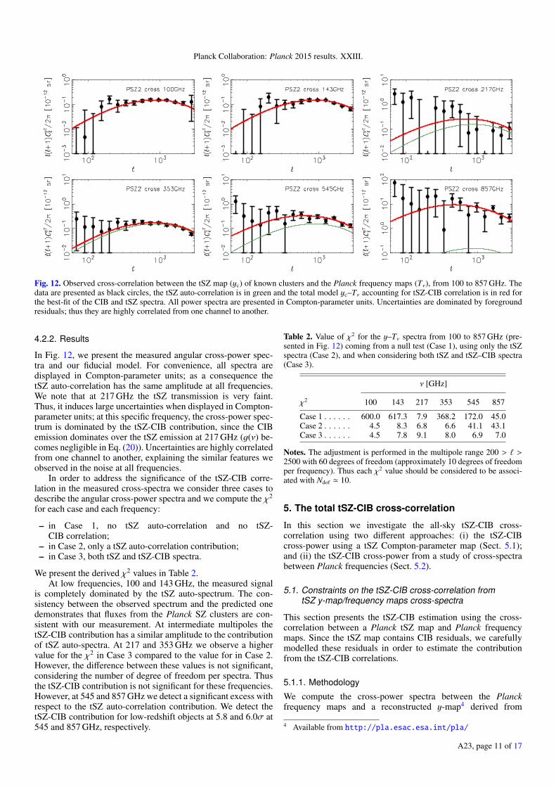
Fig. 12. Observed cross-correlation between the tSZ map (yc) of known clusters and the Planck frequency maps (Tν), from 100 to 857 GHz. Thedata are presented as black circles, the tSZ auto-correlation is in green and the total model yc–Tν accounting for tSZ-CIB correlation is in red forthe best-fit of the CIB and tSZ spectra. All power spectra are presented in Compton-parameter units. Uncertainties are dominated by foregroundresiduals; thus they are highly correlated from one channel to another.

4.2.2. Results

In Fig. 12, we present the measured angular cross-power spec-tra and our fiducial model. For convenience, all spectra aredisplayed in Compton-parameter units; as a consequence thetSZ auto-correlation has the same amplitude at all frequencies.We note that at 217 GHz the tSZ transmission is very faint.Thus, it induces large uncertainties when displayed in Compton-parameter units; at this specific frequency, the cross-power spec-trum is dominated by the tSZ-CIB contribution, since the CIBemission dominates over the tSZ emission at 217 GHz (g(ν) be-comes negligible in Eq. (20)). Uncertainties are highly correlatedfrom one channel to another, explaining the similar features weobserved in the noise at all frequencies.

In order to address the significance of the tSZ-CIB corre-lation in the measured cross-spectra we consider three cases todescribe the angular cross-power spectra and we compute the χ2

for each case and each frequency:

– in Case 1, no tSZ auto-correlation and no tSZ-CIB correlation;

– in Case 2, only a tSZ auto-correlation contribution;– in Case 3, both tSZ and tSZ-CIB spectra.

We present the derived χ2 values in Table 2.At low frequencies, 100 and 143 GHz, the measured signal

is completely dominated by the tSZ auto-spectrum. The con-sistency between the observed spectrum and the predicted onedemonstrates that fluxes from the Planck SZ clusters are con-sistent with our measurement. At intermediate multipoles thetSZ-CIB contribution has a similar amplitude to the contributionof tSZ auto-spectra. At 217 and 353 GHz we observe a highervalue for the χ2 in Case 3 compared to the value for in Case 2.However, the difference between these values is not significant,considering the number of degree of freedom per spectra. Thusthe tSZ-CIB contribution is not significant for these frequencies.However, at 545 and 857 GHz we detect a significant excess withrespect to the tSZ auto-correlation contribution. We detect thetSZ-CIB contribution for low-redshift objects at 5.8 and 6.0σ at545 and 857 GHz, respectively.

Table 2. Value of χ2 for the y–Tν spectra from 100 to 857 GHz (pre-sented in Fig. 12) coming from a null test (Case 1), using only the tSZspectra (Case 2), and when considering both tSZ and tSZ–CIB spectra(Case 3).

ν [GHz]

χ2 100 143 217 353 545 857

Case 1 . . . . . . 600.0 617.3 7.9 368.2 172.0 45.0Case 2 . . . . . . 4.5 8.3 6.8 6.6 41.1 43.1Case 3 . . . . . . 4.5 7.8 9.1 8.0 6.9 7.0

Notes. The adjustment is performed in the multipole range 200 > ` >2500 with 60 degrees of freedom (approximately 10 degrees of freedomper frequency). Thus each χ2 value should be considered to be associ-ated with Ndof ' 10.

5. The total tSZ-CIB cross-correlation

In this section we investigate the all-sky tSZ-CIB cross-correlation using two different approaches: (i) the tSZ-CIBcross-power using a tSZ Compton-parameter map (Sect. 5.1);and (ii) the tSZ-CIB cross-power from a study of cross-spectrabetween Planck frequencies (Sect. 5.2).

5.1. Constraints on the tSZ-CIB cross-correlation fromtSZ y-map/frequency maps cross-spectra

This section presents the tSZ-CIB estimation using the cross-correlation between a Planck tSZ map and Planck frequencymaps. Since the tSZ map contains CIB residuals, we carefullymodelled these residuals in order to estimate the contributionfrom the tSZ-CIB correlations.

5.1.1. Methodology

We compute the cross-power spectra between the Planckfrequency maps and a reconstructed y-map4 derived from

4 Available from http://pla.esac.esa.int/pla/

A23, page 11 of 17

A&A 594, A23 (2016)

Fig. 13. Predicted CIB transmission in the tSZ y-map for a hypotheticalCIB emission of 1 KCMB at 545 GHz and at redshift z. The shaded arearepresents the 68% confidence region, for uncertainties of ∆Td = 2 Kand ∆βd = 0.1 in the modified blackbody parameters of the hypotheticalCIB emission.

component separation (see Planck Collaboration XXII 2016, andreferences therein). We choose the MILCA map and check thatthere are no significant differences with the NILC map (bothmaps are described in Planck Collaboration XXII 2016). Thiscross-correlation can be decomposed into four terms:

Cy,Tν`

= g(ν)Cy,y`

+ Cy,CIB(ν)`

+ g(ν)Cy,yCIB`

+ CyCIB,CIB(ν)`

, (23)

where yCIB is the CIB contamination in the tSZ map. We com-pute the uncertainties as

cov(Cy,Tν`

,Cy,T ′ν`

) =Cy,y`

CTν,T ′ν`

+ Cy,Tν`

Cy,T ′ν`

(2` + 1) fsky, (24)

where fsky is the fraction of the sky that is unmasked. We binthe cross-power spectrum and deconvolve the beam and maskeffects, then we propagate uncertainties as described in Sect. 4.2.

The cross-correlations of a tSZ-map built from component-separation algorithms and Planck frequency maps are sensitiveto both the tSZ auto-correlation and tSZ-CIB cross-correlation.But this cross-correlation also has a contribution produced by theCIB contamination to the tSZ map. In particular, this contamina-tion is, by construction, highly correlated with the CIB signal inthe frequency maps.

5.1.2. Estimation of CIB leakage in the tSZ map

The tSZ maps, denoted y in the following, are derived usingcomponent-separation methods. They are constructed through alinear combination of Planck frequency maps that depends onthe angular scale and the pixel, p, as

y =∑i, j,ν

wi,p,νTi,p(ν). (25)

Here Ti,p(ν) is the Planck map at frequency ν for the angularfilter i, and wi,p,ν are the weights of the linear combination. Then,the CIB contamination in the y-map is

yCIB =∑i, j,ν

wi,p(ν)T CIBi,p (ν), (26)

where T CIB(ν) is the CIB emission at frequency ν. Using theweights wi,p,ν, and considering the CIB luminosity function, it

Fig. 14. Expected contribution to the tSZ power spectrum for the truetSZ signal (black curve), for CIB leakage (red curve), and for tSZ-CIBleakage contribution (blue curve). The dotted line indicates a negativepower spectrum.

is possible to predict the expected CIB leakage as a function ofthe redshift of the source by propagating the SED through theweights that are used to build the tSZ map.

In Fig. 13, we present the expected transmission ofCIB emission in the Planck tSZ map for a 1 KCMB CIB sourceat 545 GHz at redshift z, based on the fiducial model for thescaling relation presented in Sect. 2. The intensity of CIB leak-age in the tSZ map is given by the integration of the product ofCIB transmission (presented in Fig. 13) and the CIB scaling re-lation at 545 GHz. Error bars account for SED variation betweensources. In this case we assume an uncertainty of ∆Td = 2 K and∆βd = 0.1 on the modified blackbody parameters. We observethat the CIB at low z leaks into the tSZ map with only a smallamplitude, whereas higher-redshift CIB produces a higher, dom-inant, level of leakage. Indeed, ILC-based component-separationmethods tend to focus on Galactic thermal dust removal, andthus are less efficient at subtracting high-z CIB sources that havea different SED.

The CIB power spectra have been constrained in previousPlanck analyses (see, e.g., Planck Collaboration XVIII 2011;Planck Collaboration XXX 2014), as presented in Sect. 2.5. Wecan use this knowledge of the CIB power spectra to predict theexpected CIB leakage, yCIB, in the tSZ map, y. We performed200 Monte Carlo simulations of tSZ and CIB maps that followthe tSZ, CIB, and tSZ-CIB power spectra. Then, we applied tothese simulations the weights used to build the tSZ map. Finally,we estimated the CIB leakage and its correlation with the tSZ ef-fect. The tSZ map signal, y, can be written as y = y+yCIB. Thus,the spectrum of the tSZ map is Cy,y

`= Cy,y

`+ CyCIB,yCIB

`+ 2Cy,yCIB

`.

In Fig. 14, we present the predicted contributions to the tSZmap’s power spectrum for tSZ, CIB leakage, and tSZ-CIB leak-age. We observe that at low ` (below 400) the tSZ signal domi-nates CIB leakage and tSZ-CIB leakage contamination, whereasfor higher ` the signal is dominated by the CIB leakage part. ThetSZ-CIB leakage spectrum (dotted line in the figure) is negative,since it is dominated by low-z (z <∼ 2) CIB leakage.

We also estimate the uncertainties on CyCIB,yCIB`

, usingthe uncertainty on the CIB correlation matrix from PlanckCollaboration XXX (2014). We derive an average uncertaintyof 50% on the CIB leakage amplitude in the tSZ map. This un-certainty is correlated between multipoles at a level above 90%.Consequently, the uncertainty on the CIB leakage in the tSZ-mapcan be modelled as an overall amplitude factor.

A23, page 12 of 17

Planck Collaboration: Planck 2015 results. XXIII.

Fig. 15. From left to right and top to bottom: observed cross-correlation between the MILCA y-map and the Planck frequency maps from 30 to857 GHz. In blue are the data points, in black the CIB-cleaned data points; the red solid line is the predicted signal from tSZ only and the greenline is the total expected signal from the tSZ signal and the tSZ-CIB correlation. All spectra are presented in Compton-parameter units.

Table 3. Best-fit values for the tSZ-CIB amplitude, AtSZ−CIB, using thefiducial model as reference.

ν [GHz] AtSZ−CIB ∆AtSZ−CIB

100 . . . . . . . . −3.6 3.8143 . . . . . . . . −1.6 3.7353 . . . . . . . . 2.0 2.0545 . . . . . . . . 1.7 1.4857 . . . . . . . . 1.6 0.7

5.1.3. Results

By cross-correlating the simulated CIB leakage signal with thesimulated CIB at each frequency, it is also possible to predict theCIB leakage in the cross-spectra between tSZ map and Planckfrequency maps. We can correct Cy,Tν

`spectra (Eq. (23)) using the

estimated tSZ-CIB leakage cross-correlation term, g(ν)Cy,yCIB`

,and the CIB-CIB leakage cross-correlation term, CyCIB,CIB(ν)

`,

giving

Cy,Tν,corr`

= Cy,Tν`− g(ν)Cy,yCIB

`−CyCIB,CIB(ν)

`. (27)

Thus, the only remaining contributions are from the tSZ auto-correlation and the tSZ-CIB cross-correlation. We also propagatethe associated uncertainties.

Figure 15 shows the cross-correlation of the tSZ-map andPlanck frequency maps after correcting for the effects of thebeam and mask, and for the terms g(ν)Cy,yCIB

`and CyCIB,CIB(ν)

`.

As was the case for Fig. 12, all spectra are displayed intSZ Compton-parameter units, and the uncertainties present ahigh degree of correlation from one frequency to another. Foreach cross-spectrum we adjust the amplitude, AtSZ−CIB, of thetSZ-CIB contribution through a linear fit. The results of the fitare listed in Table 3. We obtain a maximum significance of 2.3σat 857 GHz and the results are consistent with the fiducial model.

The combined constraints from 353, 545, and 857 GHz mea-surements, as well as the covariance structure of the measure-ment uncertainties, yield an estimate of AtSZ−CIB = 1.3 ± 0.4.

The uncertainties are dominated by CIB leakage subtraction,which leads to highly correlated uncertainties of the 353, 545,and 857 GHz spectra. The optimal linear estimator we use tocalculate AtSZ−CIB probes the measurements for the known fre-quency trend of the CIB leakage in order to correct for this.Since the CIB leakage has affected all three of these correlatedmeasurements in the same direction, the combined constraintof 1.3 ± 0.4 is below the range of the individual (uncorrected)constraints ranging from 1.6 to 2.0. Table 3 contains the neces-sary covariance information used here.

5.2. Constraints on tSZ-CIB cross-correlation from Planckfrequency maps

As a last approach, we explore the direct cross-correlationbetween Planck frequency maps.

5.2.1. Methodology

In terms of tSZ and CIB components the cross-spectra betweenfrequencies ν and ν′ can be written as

Cν,ν′

`= g(ν)g(ν′)Cy,y

`+ CCIB(ν),CIB(ν′)

`+ g(ν)Cy,CIB(ν′)

`

+g(ν′)Cy,CIB(ν)`

+ Cother` (ν), (28)

where Cother` (ν) accounts for the contribution of all components

except for tSZ and CIB. We compute the cross-spectra betweenPlanck frequency maps from 100 to 857 GHz as

Cν,ν′

`=

Cν1,ν′2

`+ Cν2,ν

′1

`

2, (29)

where subscripts 1 and 2 label the “half-ring” Planck maps. Thisprocess enables us to produce power spectra without the noise

A23, page 13 of 17

A&A 594, A23 (2016)

contribution. We also compute the covariance between spectra as

cov(Cν,ν′

`,Cν′′,ν′′′

`) =

Cν1,ν′′1

`Cν′2,ν

′′′2

`+ Cν1,ν

′′′2

`Cν′2,ν

′′1

`

4(2` + 1) fsky

+Cν1,ν

′′2

`Cν′2,ν

′′′1

`+ Cν1,ν

′′′1

`Cν′2,ν

′′2

`

4(2` + 1) fsky

+Cν2,ν

′′1

`Cν′1,ν

′′′2

`+ Cν2,ν

′′′2

`Cν′1,ν

′′1

`

4(2` + 1) fsky

+Cν2,ν

′′2

`Cν′1,ν

′′′1

`+ Cν2,ν

′′′1

`Cν′1,ν

′′2

`

4(2` + 1) fsky· (30)

We correct the cross-spectra for beam and mask effects, usingthe same Galactic mask as in Sect. 4.2, removing 60% of thesky, and we propagate uncertainties on cross-power spectra asdescribed in Sect. 4.2.

The tSZ and CIB contributions to Cν,ν′

`are contaminated

by other astrophysical emission. We remove the CMB con-tribution in Cν,ν′

`using the Planck best-fit cosmology (Planck

Collaboration XIII 2016). We note that the Planck CMB mapssuffer from tSZ and CIB residuals, so they cannot be used forour purpose.

5.2.2. Estimation of tSZ-CIB amplitude

We fit thermal dust, radio sources, tSZ, CIB (that accounts forthe total fluctuations in extragalactic infrared emission), andtSZ-CIB amplitudes, Adust, Arad, AtSZ, ACIB, and AtSZ−CIB, re-spectively, through a linear fit. For the dust spectrum we as-sume C` ∝ `−2.8 (Planck Collaboration XXX 2014), and forradio sources C` ∝ ` 0. For the tSZ-CIB correlation, tSZ, andCIB power spectra, we use templates computed as presented inSect. 2.3. This gives us

Cν,ν′

`= AtSZg(ν)g(ν′)Cy,y

`

+ ACIBCCIB(ν),CIB(ν′)`

+ AtSZ−CIB

[g(ν)Cy,CIB(ν′)

`+ g(ν′)Cy,CIB(ν)

`

]+ Adust fdust(ν) fdust(ν′)`−2.8

+ Arad frad(ν) frad(ν′). (31)

Here fdust and frad give the frequency dependence of thermaldust and radio point sources, respectively. For thermal dust weassume a modified blackbody emission law, with βd = 1.55and Td = 20.8 K (Planck Collaboration XI 2014). For radiopoint sources we assume a spectral index αr = −0.7 (PlanckCollaboration XXVIII 2014). The adjustment of the amplitudesand the estimation of the amplitude covariance matrix are per-formed simultaneously on the six auto-spectra and 15 cross-spectra from ` = 50 to ` = 2000.

For tSZ and CIB spectra we reconstruct amplitudes compat-ible with previous constraints (see Sect. 2.5): ACIB = 0.98± 0.03for the CIB; and AtSZ = 1.01±0.05 for tSZ. For the tSZ-CIB con-tribution we obtain AtSZ−CIB = 1.19 ± 0.30. Thus, we obtaina detection of the tSZ-CIB cross-correlation at 4σ, consistentwith the model. In Fig. 16, we present the correlation matrixbetween cross-spectra component amplitudes. The highest de-generacy occurs between tSZ and tSZ-CIB amplitudes, with acorrelation of −50%. We also note that CIB and radio contri-butions are significantly degenerate, with tSZ-CIB correlationamplitudes of −28% and 29%, respectively.

Fig. 16. Correlation matrix for multi-frequency cross-spectracomponents from Eq. (31).

6. Conclusions and discussion

We have performed a comprehensive analysis of the infraredemission from galaxy clusters. We have proposed a model ofthe tSZ-CIB correlation derived from coherent modelling of boththe tSZ and CIB at galaxy clusters. We have shown that the mod-els of the tSZ and CIB power spectra reproduce fairly well theobserved power spectra from the Planck data. Using this ap-proach, we have been able to predict the expected tSZ-CIB cross-spectrum. Our predictions are consistent with previous work re-ported in the literature (Addison et al. 2012; Zahn et al. 2012).

We have demonstrated that the CIB scaling relation fromPlanck Collaboration XXX (2014) is able to reproduce the ob-served stacked SED of Planck confirmed clusters. We have alsoset constraints on the profile of the this emission and found thatthe infrared emission is more extended than the tSZ profile. Wealso find that the infrared profile is more extended than seen inprevious work (see e.g., Xia et al. 2012) based on numerical sim-ulation (Bullock et al. 2001). Fitting for the concentration of anNFW profile, the infrared emission shows c500 = 1.00+0.18

−0.15. Thisdemonstrates that the infrared brightness of cluster-core galaxiesis lower than that of outlying galaxies.

We have presented three distinct approaches for constrain-ing the tSZ-CIB cross-correlation level: (i) using confirmedtSZ clusters; (ii) through cross-correlating a tSZ Compton pa-rameter map with Planck frequency maps; and (iii) by directlycross-correlating Planck frequency maps. We have comparedthese analyses with the predictions from the model and de-rived consistent results. We obtain: (i) a detection of the tSZ-IR correlation at 6σ; (ii) an amplitude AtSZ−CIB = 1.5 ± 0.5;and (iii) an amplitude AtSZ−CIB = 1.2 ± 0.3. At 143 GHz thesevalues correspond to correlation coefficients at ` = 3000 of:(ii) ρ = 0.18 ± 0.07; and (iii) ρ = 0.16 ± 0.04. These resultsare consistent with previous analyses by the ACT collaboration,which set upper limits ρ < 0.2 (Dunkley et al. 2013) and bythe SPT collaboration, which found ρ = 0.11+0.06

−0.05 (George et al.2015).

Our results, with a detection of the full tSZ-CIB cross-correlation amplitude at 4σ, provide the tightest constraint so

A23, page 14 of 17

Planck Collaboration: Planck 2015 results. XXIII.

far on the tSZ-CIB correlation factor. Such constraints on thetSZ-CIB cross-correlation are needed to perform an accuratemeasurement of the tSZ power spectrum. Beyond power spec-trum analyses, the tSZ-CIB cross-correlation is also a majorissue for relativistic tSZ studies, since CIB emission towardgalaxy clusters mimics the relativistic tSZ correction and thuscould produce significant bias if not accounted for properly. This4σ measurement of the amplitude of the tSZ-CIB correlationwill also be important for estimates of the “kinetic” SZ powerspectrum.

Acknowledgements. The Planck Collaboration acknowledges the supportof: ESA; CNES, and CNRS/INSU-IN2P3-INP (France); ASI, CNR, andINAF (Italy); NASA and DoE (USA); STFC and UKSA (UK); CSIC,MINECO, JA and RES (Spain); Tekes, AoF, and CSC (Finland); DLRand MPG (Germany); CSA (Canada); DTU Space (Denmark); SER/SSO(Switzerland); RCN (Norway); SFI (Ireland); FCT/MCTES (Portugal); ERCand PRACE (EU). A description of the Planck Collaboration and a list ofits members, indicating which technical or scientific activities they have beeninvolved in, can be found at http://www.cosmos.esa.int/web/planck/planck-collaboration. Some of the results in this paper have been derivedusing the HEALPix package. We also acknowledge the support of the FrenchAgence Nationale de la Recherche under grant ANR-11-BD56-015.

ReferencesAddison, G. E., Dunkley, J., & Spergel, D. N. 2012, MNRAS, 427, 1741Aghanim, N., Hurier, G., Diego, J.-M., et al. 2015, A&A, 580, A138Amblard, A., Cooray, A., Serra, P., et al. 2011, Nature, 470, 510Arnaud, M., Pratt, G. W., Piffaretti, R., et al. 2010, A&A, 517, A92Birkinshaw, M. 1999, Phys. Rep., 310, 97Braglia, F. G., Ade, P. A. R., Bock, J. J., et al. 2011, MNRAS, 412, 1187Bullock, J. S., Kolatt, T. S., Sigad, Y., et al. 2001, MNRAS, 321, 559Carlstrom, J. E., Holder, G. P., & Reese, E. D. 2002, ARA&A, 40, 643Cooray, A., & Sheth, R. 2002, Phys. Rep., 372, 1Coppin, K. E. K., Geach, J. E., Smail, I., et al. 2011, MNRAS, 416, 680Diego, J. M., & Partridge, B. 2009, ArXiv e-prints [arXiv:0907.0233]Dunkley, J., Hlozek, R., Sievers, J., et al. 2011, ApJ, 739, 52Dunkley, J., Calabrese, E., Sievers, J., et al. 2013, J. Cosmol. Astropart. Phys.,

7, 25Fixsen, D. J., Dwek, E., Mather, J. C., Bennett, C. L., & Shafer, R. A., 1998,

ApJ, 508, 123George, E. M., Reichardt, C. L., Aird, K. A., et al. 2015, ApJ, 799, 177Giard, M., Montier, L., Pointecouteau, E., & Simmat, E. 2008, A&A, 490, 547Górski, K. M., Hivon, E., Banday, A. J., et al. 2005, ApJ, 622, 759Hall, N. R., Keisler, R., Knox, L., et al. 2010, ApJ, 718, 632Halverson, N. W., Lanting, T., Ade, P. A. R., et al. 2009, ApJ, 701, 42Hauser, M. G., & Dwek, E. 2001, ARA&A, 39, 249Hauser, M. G., Arendt, R. G., Kelsall, T., et al. 1998, ApJ, 508, 25Hincks, A. D., Acquaviva, V., Ade, P. A. R., et al. 2010, ApJS, 191, 423Hurier, G., Aghanim, N., Douspis, M., & Pointecouteau, E. 2014, A&A, 561,

A143Kennicutt, Jr., R. C. 1998, ARA&A, 36, 189Komatsu, E., & Kitayama, T. 1999, ApJ, 526, L1Komatsu, E., & Seljak, U. 2002, MNRAS, 336, 1256Lagache, G., Puget, J.-L., & Dole, H. 2005, ARA&A, 43, 727Lagache, G., Bavouzet, N., Fernandez-Conde, N., et al. 2007, ApJ, 665, L89Lesgourgues, J. 2011, ArXiv e-prints [arXiv:1104.2932]Lieu, R., Mittaz, J. P. D., & Zhang, S.-N. 2006, ApJ, 648, 176Mesinger, A., McQuinn, M., & Spergel, D. N. 2012, MNRAS, 422, 1403Miville-Deschênes, M.-A., & Lagache, G. 2005, ApJS, 157, 302Mo, H. J., & White, S. D. M. 1996, MNRAS, 282, 347Montier, L. A., & Giard, M. 2005, A&A, 439, 35Muzzin, A., van der Burg, R. F. J., McGee, S. L., et al. 2014, ApJ, 796, 65Nagai, D., Kravtsov, A. V., & Vikhlinin, A. 2007, ApJ, 668, 1Navarro, J. F., Frenk, C. S., & White, S. D. M. 1997, ApJ, 490, 493Planck Collaboration X. 2011, A&A, 536, A10Planck Collaboration XI. 2011, A&A, 536, A11Planck Collaboration XVIII. 2011, A&A, 536, A18Planck Collaboration I. 2014, A&A, 571, A1Planck Collaboration VII. 2014, A&A, 571, A7Planck Collaboration IX. 2014, A&A, 571, A9Planck Collaboration XI. 2014, A&A, 571, A11Planck Collaboration XVIII. 2014, A&A, 571, A18

Planck Collaboration XX. 2014, A&A, 571, A20Planck Collaboration XXI. 2014, A&A, 571, A21Planck Collaboration XXVIII. 2014, A&A, 571, A28Planck Collaboration XXX. 2014, A&A, 571, A30Planck Collaboration I. 2016, A&A, 594, A1Planck Collaboration II. 2016, A&A, 594, A2Planck Collaboration III. 2016, A&A, 594, A3Planck Collaboration IV. 2015, A&A, 594, A4Planck Collaboration V. 2016, A&A, 594, A5Planck Collaboration VI. 2016, A&A, 594, A6Planck Collaboration VII. 2016, A&A, 594, A7Planck Collaboration VIII. 2016, A&A, 594, A8Planck Collaboration IX. 2016, A&A, 594, A9Planck Collaboration X. 2016, A&A, 594, A10Planck Collaboration XI. 2016, A&A, 594, A11Planck Collaboration XII. 2016, A&A, 594, A12Planck Collaboration XIII. 2016, A&A, 594, A13Planck Collaboration XIV. 2016, A&A, 594, A14Planck Collaboration XV. 2016, A&A, 594, A15Planck Collaboration XVI. 2016, A&A, 594, A16Planck Collaboration XVII. 2016, A&A, 594, A17Planck Collaboration XVIII. 2016, A&A, 594, A18Planck Collaboration XIX. 2016, A&A, 594, A19Planck Collaboration XX. 2016, A&A, 594, A20Planck Collaboration XXI. 2016, A&A, 594, A21Planck Collaboration XXII. 2016, A&A, 594, A22Planck Collaboration XXIII. 2016, A&A, 594, A23Planck Collaboration XXIV. 2016, A&A, 594, A24Planck Collaboration XXV. 2016, A&A, 594, A25Planck Collaboration XXVI. 2016, A&A, 594, A26Planck Collaboration XXVII. 2016, A&A, 594, A27Planck Collaboration XXVIII. 2016, A&A, 594, A28Planck Collaboration Int. III. 2013, A&A, 550, A129Planck Collaboration Int. V. 2013, A&A, 550, A131Planck Collaboration Int. VIII. 2013, A&A, 550, A134Planck Collaboration Int. X. 2013, A&A, 554, A140Planck Collaboration Int. XXXVII. 2016, A&A, 586, A140Puget, J.-L., Abergel, A., Bernard, J.-P., et al. 1996, A&A, 308, L5Reichardt, C. L., Shaw, L., Zahn, O., et al. 2012, ApJ, 755, 70Rephaeli, Y. 1995, ARA&A, 33, 541Roncarelli, M., Pointecouteau, E., Giard, M., Montier, L., & Pello, R. 2010,

A&A, 512, A20Santos, J. S., Altieri, B., Popesso, P., et al. 2013, MNRAS, 433, 1287Sayers, J., Golwala, S. R., Ameglio, S., & Pierpaoli, E. 2011, ApJ, 728, 39Shang, C., Haiman, Z., Knox, L., & Oh, S. P. 2012, MNRAS, 421, 2832Sievers, J. L., Hlozek, R. A., Nolta, M. R., et al. 2013, J. Cosmol. Astropart.

Phys., 10, 60Sunyaev, R. A., & Zeldovich, Y. B. 1969, Nature, 223, 721Sunyaev, R. A., & Zeldovich, Y. B. 1972, Comm. Astrophys. Space Phys., 4, 173Taburet, N., Hernández-Monteagudo, C., Aghanim, N., Douspis, M., & Sunyaev,

R. A. 2011, MNRAS, 418, 2207Tinker, J. L., & Wetzel, A. R. 2010, ApJ, 719, 88Tinker, J., Kravtsov, A. V., Klypin, A., et al. 2008, ApJ, 688, 709Tinker, J. L., Robertson, B. E., Kravtsov, A. V., et al. 2010, ApJ, 724, 878Tristram, M., Macías-Pérez, J. F., Renault, C., & Santos, D. 2005, MNRAS, 358,

833Viero, M. P., Moncelsi, L., Mentuch, E., et al. 2012, MNRAS, 421, 2161Viero, M. P., Moncelsi, L., Quadri, R. F., et al. 2015, ApJ, 809, L22Weinmann, S. M., Kauffmann, G., von der Linden, A., & De Lucia, G. 2010,

MNRAS, 406, 2249Wheelock, S., Gautier, T. N., Chillemi, J., et al. 1993, Issa explanatory sup-

plement. Technical report., Issa explanatory supplement. Technical report,Infrared Processing and Analysis Center

Xia, J.-Q., Negrello, M., Lapi, A., et al. 2012, MNRAS, 422, 1324Zahn, O., Reichardt, C. L., Shaw, L., et al. 2012, ApJ, 756, 65Zwart, J. T. L., Feroz, F., Davies, M. L., et al. 2011, MNRAS, 418, 2754

1 APC, AstroParticule et Cosmologie, Université Paris Diderot,CNRS/IN2P3, CEA/lrfu, Observatoire de Paris, Sorbonne ParisCité, 10 rue Alice Domon et Léonie Duquet, 75205 Paris Cedex 13,France

2 African Institute for Mathematical Sciences, 6–8 Melrose Road,Muizenberg, Cape Town, South Africa

3 Agenzia Spaziale Italiana Science Data Center, via del Politecnicosnc, 00133 Roma, Italy

A23, page 15 of 17

A&A 594, A23 (2016)

4 Aix-Marseille Université, CNRS, LAM (Laboratoired’Astrophysique de Marseille) UMR 7326, 13388 Marseille,France

5 Astrophysics Group, Cavendish Laboratory, University ofCambridge, J J Thomson Avenue, Cambridge CB3 0HE, UK

6 Astrophysics & Cosmology Research Unit, School of Mathematics,Statistics & Computer Science, University of KwaZulu-Natal,Westville Campus, Private Bag X54001, 4000 Durban, South Africa

7 Atacama Large Millimeter/submillimeter Array, ALMA SantiagoCentral Offices, Alonso de Cordova 3107, Vitacura, Casilla763 0355, Santiago, Chile

8 CITA, University of Toronto, 60 St. George St., Toronto,ON M5S 3H8, Canada

9 CNRS, IRAP, 9 Av. colonel Roche, BP 44346, 31028 ToulouseCedex 4, France

10 California Institute of Technology, Pasadena, CA 91125, USA11 Centro de Estudios de Física del Cosmos de Aragón (CEFCA), Plaza

San Juan, 1, planta 2, 44001 Teruel, Spain12 Computational Cosmology Center, Lawrence Berkeley National

Laboratory, Berkeley, California, USA13 DSM/Irfu/SPP, CEA-Saclay, 91191 Gif-sur-Yvette Cedex, France14 DTU Space, National Space Institute, Technical University of

Denmark, Elektrovej 327, 2800 Kgs. Lyngby, Denmark15 Département de Physique Théorique, Université de Genève, 24 quai

E. Ansermet, 1211 Genève 4, Switzerland16 Departamento de Astrofísica, Universidad de La Laguna (ULL),

38206 La Laguna, Tenerife, Spain17 Departamento de Física, Universidad de Oviedo, Avda. Calvo Sotelo

s/n, Oviedo, Spain18 Department of Astrophysics/IMAPP, Radboud University

Nijmegen, PO Box 9010, 6500 GL Nijmegen, The Netherlands19 Department of Physics & Astronomy, University of British

Columbia, 6224 Agricultural Road, Vancouver, British Columbia,Canada

20 Department of Physics and Astronomy, Dana and David DornsifeCollege of Letter, Arts and Sciences, University of SouthernCalifornia, Los Angeles, CA 90089, USA

21 Department of Physics and Astronomy, University College London,London WC1E 6BT, UK

22 Department of Physics, Florida State University, Keen PhysicsBuilding, 77 Chieftan Way, Tallahassee, Florida, USA

23 Department of Physics, Gustaf Hällströmin katu 2a, University ofHelsinki, 00560 Helsinki, Finland

24 Department of Physics, Princeton University, Princeton, New Jersey,USA

25 Department of Physics, University of California, Santa Barbara,California, USA

26 Department of Physics, University of Illinois at Urbana-Champaign,1110 West Green Street, Urbana, Illinois, USA

27 Dipartimento di Fisica e Astronomia G. Galilei, Università degliStudi di Padova, via Marzolo 8, 35131 Padova, Italy

28 Dipartimento di Fisica e Scienze della Terra, Università di Ferrara,via Saragat 1, 44122 Ferrara, Italy

29 Dipartimento di Fisica, Università La Sapienza, P.le A. Moro 2,00133 Roma, Italy

30 Dipartimento di Fisica, Università degli Studi di Milano, via Celoria,16, 20133 Milano, Italy

31 Dipartimento di Fisica, Università degli Studi di Trieste, via A.Valerio 2, 34127 Trieste, Italy

32 Dipartimento di Matematica, Università di Roma Tor Vergata, viadella Ricerca Scientifica, 1, 00133 Roma, Italy

33 Discovery Center, Niels Bohr Institute, Blegdamsvej 17,Copenhagen, Denmark

34 European Southern Observatory, ESO Vitacura, Alonso de Cordova3107, Vitacura, Casilla 19001, Santiago, Chile

35 European Space Agency, ESAC, Planck Science Office, Caminobajo del Castillo, s/n, Urbanización Villafranca del Castillo, 28692Villanueva de la Cañada, Madrid, Spain

36 European Space Agency, ESTEC, Keplerlaan 1, 2201 AZNoordwijk, The Netherlands

37 Facoltà di Ingegneria, Università degli Studi e-Campus, viaIsimbardi 10, 22060 Novedrate (CO), Italy

38 Gran Sasso Science Institute, INFN, viale F. Crispi 7, 67100L’Aquila, Italy

39 HGSFP and University of Heidelberg, Theoretical PhysicsDepartment, Philosophenweg 16, 69120 Heidelberg, Germany

40 Haverford College Astronomy Department, 370 Lancaster Avenue,Haverford, Pennsylvania, USA

41 Helsinki Institute of Physics, Gustaf Hällströmin katu 2, Universityof Helsinki, 00560 Helsinki, Finland

42 INAF–Osservatorio Astrofisico di Catania, via S. Sofia 78, Catania,Italy

43 INAF–Osservatorio Astronomico di Padova, Vicolodell’Osservatorio 5, Padova, Italy

44 INAF–Osservatorio Astronomico di Roma, via di Frascati 33,Monte Porzio Catone, Italy

45 INAF–Osservatorio Astronomico di Trieste, via G.B. Tiepolo 11,Trieste, Italy

46 INAF/IASF Bologna, via Gobetti 101, 40127 Bologna, Italy47 INAF/IASF Milano, via E. Bassini 15, 20133 Milano, Italy48 INFN, Sezione di Bologna, via Irnerio 46, 40126 Bologna, Italy49 INFN, Sezione di Roma 1, Università di Roma Sapienza, P.le Aldo

Moro 2, 00185 Roma, Italy50 INFN, Sezione di Roma 2, Università di Roma Tor Vergata, via della

Ricerca Scientifica 1, 00185 Roma, Italy51 INFN/National Institute for Nuclear Physics, via Valerio 2, 34127

Trieste, Italy52 IPAG: Institut de Planétologie et d’Astrophysique de Grenoble,

Université Grenoble Alpes, IPAG, CNRS IPAG, 38000 Grenoble,France

53 IUCAA, Post Bag 4, Ganeshkhind, Pune University Campus,411 007 Pune, India

54 Imperial College London, Astrophysics group, Blackett Laboratory,Prince Consort Road, London, SW7 2AZ, UK

55 Infrared Processing and Analysis Center, California Institute ofTechnology, Pasadena, CA 91125, USA

56 Institut Universitaire de France, 103 bd Saint-Michel, 75005 Paris,France

57 Institut d’Astrophysique Spatiale, CNRS (UMR 8617) UniversitéParis-Sud 11, Bâtiment 121, 91898 Orsay, France

58 Institut d’Astrophysique de Paris, CNRS (UMR 7095), 98bis boule-vard Arago, 75014 Paris, France

59 Institute of Astronomy, University of Cambridge, Madingley Road,Cambridge CB3 0HA, UK

60 Institute of Theoretical Astrophysics, University of Oslo, Blindern,0371 Oslo, Norway

61 Instituto de Astrofísica de Canarias, C/Vía Láctea s/n, La Laguna,Tenerife, Spain

62 Instituto de Física de Cantabria (CSIC-Universidad de Cantabria),Avda. de los Castros s/n, 39005 Santander, Spain

63 Istituto Nazionale di Fisica Nucleare, Sezione di Padova, viaMarzolo 8, 35131 Padova, Italy

64 Jet Propulsion Laboratory, California Institute of Technology, 4800Oak Grove Drive, Pasadena, California, USA

65 Jodrell Bank Centre for Astrophysics, Alan Turing Building, Schoolof Physics and Astronomy, The University of Manchester, OxfordRoad, Manchester, M13 9PL, UK

66 Kavli Institute for Cosmological Physics, University of Chicago,Chicago, IL 60637, USA

67 Kavli Institute for Cosmology Cambridge, Madingley Road,Cambridge, CB3 0HA, UK

68 Kazan Federal University, 18 Kremlyovskaya St., 420008 Kazan,Russia

69 LAL, Université Paris-Sud, CNRS/IN2P3, Orsay, France70 LERMA, CNRS, Observatoire de Paris, 61 avenue de

l’Observatoire, 75000 Paris, France71 Laboratoire AIM, IRFU/Service d’Astrophysique – CEA/DSM –

CNRS – Université Paris Diderot, Bât. 709, CEA-Saclay, 91191Gif-sur-Yvette Cedex, France

A23, page 16 of 17

Planck Collaboration: Planck 2015 results. XXIII.

72 Laboratoire de Physique Subatomique et Cosmologie, UniversitéGrenoble-Alpes, CNRS/IN2P3, 53 rue des Martyrs, 38026 GrenobleCedex, France

73 Laboratoire de Physique Théorique, Université Paris-Sud 11 &CNRS, Bâtiment 210, 91405 Orsay, France

74 Lawrence Berkeley National Laboratory, Berkeley, CA 94720, USA75 Lebedev Physical Institute of the Russian Academy of Sciences,

Astro Space Centre, 84/32 Profsoyuznaya st., Moscow, GSP-7,117997, Russia

76 Max-Planck-Institut für Astrophysik, Karl-Schwarzschild-Str. 1,85741 Garching, Germany

77 National University of Ireland, Department of ExperimentalPhysics, Maynooth, Co. Kildare, Ireland

78 Nicolaus Copernicus Astronomical Center, Bartycka 18, 00-716Warsaw, Poland

79 Niels Bohr Institute, Blegdamsvej 17, Copenhagen, Denmark80 Optical Science Laboratory, University College London, Gower

Street, London WC1E 6BT, UK81 SISSA, Astrophysics Sector, via Bonomea 265, 34136 Trieste, Italy82 School of Physics and Astronomy, Cardiff University, Queens

Buildings, The Parade, Cardiff, CF24 3AA, UK

83 Sorbonne Université-UPMC, UMR 7095, Institut d’Astrophysiquede Paris, 98bis boulevard Arago, 75014 Paris, France

84 Space Research Institute (IKI), Russian Academy of Sciences,Profsoyuznaya Str, 84/32, 117997 Moscow, Russia

85 Space Sciences Laboratory, University of California, Berkeley,California, USA

86 Special Astrophysical Observatory, Russian Academy of Sciences,Nizhnij Arkhyz, Zelenchukskiy region, 369167 Karachai-Cherkessian Republic, Russia

87 Sub-Department of Astrophysics, University of Oxford, KebleRoad, Oxford OX1 3RH, UK

88 UPMC Univ. Paris 06, UMR 7095, 98bis boulevard Arago, 75014Paris, France

89 Université de Toulouse, UPS-OMP, IRAP, 31028 Toulouse Cedex 4,France

90 University of Granada, Departamento de Física Teórica y delCosmos, Facultad de Ciencias, 18010 Granada, Spain

91 University of Granada, Instituto Carlos I de Física Teórica yComputacional, 18010 Granada, Spain

92 Warsaw University Observatory, Aleje Ujazdowskie 4, 00-478Warszawa, Poland

A23, page 17 of 17