A&A 550, A132 (2013)DOI: 10.1051/0004-6361/201220039c© ESO 2013

Astronomy&

Astrophysics

Planck intermediate resultsVI. The dynamical structure of PLCKG214.6+37.0, a Planck discovered triple

system of galaxy clusters

Planck Collaboration: P. A. R. Ade88, N. Aghanim60, M. Arnaud75, M. Ashdown72,7, F. Atrio-Barandela20,J. Aumont60, C. Baccigalupi87, A. Balbi38, A. J. Banday97,10, R. B. Barreiro68, J. G. Bartlett1,69, E. Battaner99,K. Benabed61,95, A. Benoît58, J.-P. Bernard10, M. Bersanelli36,52, R. Bhatia8, I. Bikmaev22,3, H. Böhringer81,

A. Bonaldi70, J. R. Bond9, J. Borrill15,91, F. R. Bouchet61,95, H. Bourdin38, R. Burenin89, C. Burigana51,34, P. Cabella39,J.-F. Cardoso76,1,61, G. Castex1, A. Catalano77,74, L. Cayón32, A. Chamballu56, L.-Y Chiang64, G. Chon81,

P. R. Christensen84,40, D. L. Clements56, S. Colafrancesco48, S. Colombi61,95, L. P. L. Colombo25,69, B. Comis77,A. Coulais74, B. P. Crill69,85, F. Cuttaia51, A. Da Silva13, H. Dahle66,12, L. Danese87, R. J. Davis70, P. de Bernardis35,

G. de Gasperis38, G. de Zotti47,87, J. Delabrouille1, J. Démoclès75, J. M. Diego68, K. Dolag98,80, H. Dole60,59,S. Donzelli52, O. Doré69,11, U. Dörl80, M. Douspis60, X. Dupac43, G. Efstathiou65, T. A. Enßlin80, H. K. Eriksen66,

F. Finelli51, I. Flores-Cacho10,97, O. Forni97,10, M. Frailis49, E. Franceschi51, M. Frommert19, S. Galeotta49, K. Ganga1,R. T. Génova-Santos67, M. Giard97,10, M. Gilfanov80,90, Y. Giraud-Héraud1, J. González-Nuevo68,87,

K. M. Górski69,100, A. Gregorio37,49, A. Gruppuso51, F. K. Hansen66, D. Harrison65,72, P. Heinämäki94, A. Hempel67,41,S. Henrot-Versillé73, C. Hernández-Monteagudo14,80, D. Herranz68, S. R. Hildebrandt11, E. Hivon61,95, M. Hobson7,

W. A. Holmes69, G. Hurier77, T. R. Jaffe97,10, A. H. Jaffe56, T. Jagemann43, W. C. Jones27, M. Juvela26, E. Keihänen26,I. Khamitov93, T. S. Kisner79, R. Kneissl42,8, J. Knoche80, L. Knox29, M. Kunz19,60,4, H. Kurki-Suonio26,46,

G. Lagache60, A. Lähteenmäki2,46, J.-M. Lamarre74, A. Lasenby7,72, C. R. Lawrence69, M. Le Jeune1, R. Leonardi43,P. B. Lilje66,12, M. López-Caniego68, G. Luzzi73, J. F. Macías-Pérez77, D. Maino36,52, N. Mandolesi51,6,34, M. Maris49,

F. Marleau63, D. J. Marshall75, E. Martínez-González68, S. Masi35, M. Massardi50, S. Matarrese33, P. Mazzotta38,S. Mei45,96,11, A. Melchiorri35,53, J.-B. Melin17, L. Mendes43, A. Mennella36,52, S. Mitra55,69,

M.-A. Miville-Deschênes60,9, A. Moneti61, L. Montier97,10, G. Morgante51, D. Mortlock56, D. Munshi88,J. A. Murphy83, P. Naselsky84,40, F. Nati35, P. Natoli34,5,51, H. U. Nørgaard-Nielsen18, F. Noviello70, D. Novikov56,

I. Novikov84, S. Osborne92, F. Pajot60, D. Paoletti51, F. Pasian49, G. Patanchon1, O. Perdereau73, L. Perotto77,F. Perrotta87, F. Piacentini35, M. Piat1, E. Pierpaoli25, R. Piffaretti75,17, S. Plaszczynski73, E. Pointecouteau97,10,

G. Polenta5,48, N. Ponthieu60,54, L. Popa62, T. Poutanen46,26,2, G. W. Pratt75, S. Prunet61,95, J.-L. Puget60,J. P. Rachen23,80, R. Rebolo67,16,41, M. Reinecke80, M. Remazeilles60,1, C. Renault77, S. Ricciardi51, T. Riller80,

I. Ristorcelli97,10, G. Rocha69,11, M. Roman1, C. Rosset1, M. Rossetti36,52,?, J. A. Rubiño-Martín67,41, B. Rusholme57,M. Sandri51, G. Savini86, D. Scott24, G. F. Smoot28,79,1, J.-L. Starck75, R. Sudiwala88, R. Sunyaev80,90, D. Sutton65,72,

A.-S. Suur-Uski26,46, J.-F. Sygnet61, J. A. Tauber44, L. Terenzi51, L. Toffolatti21,68, M. Tomasi52, M. Tristram73,J. Tuovinen82, L. Valenziano51, B. Van Tent78, P. Vielva68, F. Villa51, N. Vittorio38, L. A. Wade69, B. D. Wandelt61,95,31,

N. Welikala60, D. Yvon17, A. Zacchei49, S. Zaroubi71, and A. Zonca30

(Affiliations can be found after the references)

Received 17 July 2012 / Accepted 22 October 2012

ABSTRACT

The survey of galaxy clusters performed by Planck through the Sunyaev-Zeldovich effect has already discovered many interesting objects, thanks toits full sky coverage. One of the SZ candidates detected in the early months of the mission near to the signal-to-noise threshold, PLCKG214.6+37.0,was later revealed by XMM-Newton to be a triple system of galaxy clusters. We present the results from a deep XMM-Newton re-observation ofPLCKG214.6+37.0, part of a multi-wavelength programme to investigate Planck discovered superclusters. The characterisation of the physicalproperties of the three components has allowed us to build a template model to extract the total SZ signal of this system with Planck data. We havepartly reconciled the discrepancy between the expected SZ signal derived from X-rays and the observed one, which are now consistent within 1.2σ.We measured the redshift of the three components with the iron lines in the X-ray spectrum, and confirm that the three clumps are likely part ofthe same supercluster structure. The analysis of the dynamical state of the three components, as well as the absence of detectable excess X-rayemission, suggests that we are witnessing the formation of a massive cluster at an early phase of interaction.

Key words. galaxies: clusters: general – large-scale structure of Universe – galaxies: clusters: individual: PLCKG214.6+37.0

? Corresponding author: M. Rossetti, e-mail: mariachiara.rossetti@unimi.it

Article published by EDP Sciences A132, page 1 of 14

A&A 550, A132 (2013)

1. Introduction

Clusters of galaxies occupy a special position in the hierarchy ofcosmic structures, because they are the largest objects that de-coupled from the cosmic expansion and that have had time toundergo gravitational collapse. They are thought to form via ahierarchical sequence of mergers and accretion of smaller sys-tems driven by gravity. During this process the intergalactic gasis heated to high X-ray emitting temperatures by adiabatic com-pression and shocks and settles in hydrostatic equilibrium withinthe cluster potential well. Sometimes galaxy clusters are foundin multiple systems, super-cluster structures that already decou-pled from the Hubble flow and are destined to collapse. Thecrowded environment of superclusters is an ideal place to studythe merging processes of individual components at an early stageof merging and to witness the initial formation phase of verymassive structures. Moreover, the processes related to the con-traction may increase the density of the intercluster medium andmake it observable with current instruments. An example is thecentral complex of the Shapley concentration, which has beenthe object of extensive multi-wavelength observations with theaim of characterising the merger processes in galaxy clusters(e.g. Kull & Böhringer 1999; Bardelli et al. 1998; Rossetti et al.2007; Giacintucci et al. 2005).

Recently a new observational window has opened up for thestudy of the astrophysics of galaxy clusters through the Sunyaev-Zeldovich effect (Sunyaev & Zeldovich 1972, SZ hereafter): aspectral distortion of the cosmic microwave background (CMB)generated through inverse Compton scattering of CMB photonsby thermal electrons in the intracluster medium (ICM). SZ sur-veys are discovering new clusters, some of which are interestingmerging systems (with “El Gordo”, Menanteau et al. 2012, beingprobably the most spectacular example).

A key role in SZ science is now played by the Planck1 satel-lite. Compared to other SZ surveys of galaxy clusters, Planckhas only moderate band-dependent spatial resolution, but it pos-sesses a unique nine-band coverage, and more crucially it cov-ers the whole sky. Therefore, it allows the rarest objects to bedetected: massive high-redshift systems (Planck Collaboration2011f), which are the most sensitive to cosmology; and com-plex multiple systems, which are interesting for the physics ofstructure formation. Indeed, during the follow-up XMM-Newtoncampaign of Planck SZ candidates, we found two new dou-ble systems and two new triple systems of clusters (PlanckCollaboration 2011c, hereafter Paper I). In all cases, the cumu-lative contribution predicted by X-ray measurements was lowerthan the measured SZ signal, although compatible within 3σ.

PLCKG214.6+37.0 is the most massive and the X-raybrightest of the two Planck discovered triple systems. TheXMM-Newton follow-up observations showed that the PlanckSZ source candidate position is located ∼5′ from the two south-ern components (A and B). A third subcomponent, C, liesapproximately 7′ to the north (Fig. 1). The X-ray spectral anal-ysis of component A indicated a redshift of zFe ∼ 0.45, con-sistent with two galaxies with spectroscopic redshift of ∼0.45,close to the peaks of components A and C. A cross-correlationwith SDSS-DR7 luminous red galaxies and the supercluster cat-alogue from the SDSS-DR7 (Liivamägi et al. 2012) hinted that

1 Planck (http://www.esa.int/Planck) is a project of theEuropean Space Agency (ESA) with instruments provided by two sci-entific consortia funded by ESA member states (in particular the leadcountries: France and Italy) with contributions from NASA (USA), andtelescope reflectors provided in a collaboration between ESA and a sci-entific consortium led and funded by Denmark.

this triple system is encompassed within a very large-scale struc-ture located at z ∼ 0.45, and whose centroid lies about 2 deg tothe south (see Appendix B in Paper I for further details).

In this paper we present new SZ measurements of this objectwith Planck and compare them with the results from a a deepXMM-Newton re-observation. In Sect. 2 we describe the analy-sis methods and the Planck and XMM-Newton data used in thispaper. In Sect. 3 we present our results obtained with X-ray and,in Sect. 4, compare them with available optical data from SDSS.In Sect. 5 we compare the X-ray results with Planck results. InSect. 6 we discuss our findings.

Throughout the paper we adopt a ΛCDM cosmology withH0 = 70 km s−1 Mpc−1, ΩM = 0.3, and ΩΛ = 0.7. At thenominal redshift of the supercluster, z = 0.45, one arcminutecorresponds to 350 kpc.

2. Observations

2.1. Planck data and analysis

Planck (Tauber et al. 2010; Planck Collaboration 2011a) is thethird-generation space mission to measure the anisotropy of theCMB. It observes the sky in nine frequency bands covering 30–857 GHz with high sensitivity and angular resolution from 31′to 5′. The Low Frequency Instrument (LFI; Mandolesi et al.2010; Bersanelli et al. 2010; Mennella et al. 2011) covers the30, 44, and 70 GHz bands with amplifiers cooled to 20 K. TheHigh Frequency Instrument (HFI; Lamarre et al. 2010; PlanckHFI Core Team 2011a) covers the 100, 143, 217, 353, 545, and857 GHz bands with bolometers cooled to 0.1 K. Polarisation ismeasured in all but the two highest bands (Leahy et al. 2010;Rosset et al. 2010). A combination of radiative cooling and threemechanical coolers produces the temperatures needed for the de-tectors and optics (Planck Collaboration 2011b). Two data pro-cessing centres (DPCs) check and calibrate the data and makemaps of the sky (Planck HFI Core Team 2011b; Zacchei et al.2011). Planck’s sensitivity, angular resolution, and frequencycoverage make it a powerful instrument for Galactic and ex-tragalactic astrophysics, as well as for cosmology. Early astro-physics results are given in Planck Collaboration (2011h–z).

Our results are based on the SZ signal as extracted from thesix bands of HFI corresponding to the nominal Planck surveyof 14 months, during which the whole sky was observed twice.We refer to Planck HFI Core Team (2011b) and Zacchei et al.(2011) for the generic scheme of TOI processing and map mak-ing, as well as for the technical characteristics of the maps used.We adopted a circular Gaussian as the beam pattern for each fre-quency, as described in Planck HFI Core Team (2011b); Zaccheiet al. (2011).

The total SZ signal is characterised by the inte-grated Compton parameter Y500 defined as D2

A(z)Y500 =

(σT/mec2)∫

PthdV , where DA(z) is the angular distance to a sys-tem at redshift z, σT is the Thomson cross-section, c the speedof light, me the rest mass of the electron, Pth the pressure ofthermal electrons, and the integral is performed over a sphere ofradius R500.

The extraction of the total SZ signal for this structure is morecomplicated than for single clusters. Owing to its moderate spa-tial resolution, Planck is not able to separate the contributions ofthe three components from the whole signal. In Paper I, we es-timated the total flux assuming a single component with masscorresponding to the sum of the masses of the three clumps,

A132, page 2 of 14

Planck Collaboration: The dynamical structure of PLCKG214.6+37.0, a Planck discovered triple system of galaxy clusters

Fig. 1. Triple systems PLCKG214.6+37.0. Left upper panel: Planck SZ reconstructed map (derived from the Modified Internal Linear CombinationAnalysis, Hurier et al. 2010), oversampled and smoothed for display purposes. Right upper panel: XMM-Newton wavelet filtered image in the[0.5–2.5] keV range (Sect. 2.2). The three components of PLCKG214.6+37.0 are marked with circles (with radius R500, see Table 1) and indicatedwith letters as in the text. The X-ray structure visible in the north-east (marked with an asterisk) is likely associated with the active galaxySDSSJ090912.15 + 144613.7, with a spectroscopic redshift z = 0.767. Left lower panel: Raw MOS count rate (counts s−1) image in the [0.5–2.5] keV range, corrected for vignetting. The black circles mark the point sources detected by our algorithm, which we masked during the analysis(Sect. 2.2). The pixel size in this image is 4.35′′. Right lower panel: SDSS r-band image of the PLCKG214.6+37.0 field. In all panels, north is upand east to the left, and we overlay X-ray contours, computed on the wavelet-filtered image logarithmically spaced starting from the level where aconnection is seen between all components (Sect. 3.4).

following a universal pressure profile (Arnaud et al. 2010) cen-tred at the barycentre of the three components. This is obviouslyonly a simple first-order approach. The wealth of informationthat is now available on this system has allowed us to build amore representative model. With the X-ray constraints on thestructural properties of clumps A, B, and C (Sect. 3.1), we arenow able to build a three-component model. As discussed inPlanck Collaboration (2011d), our baseline pressure profile isthe standard “universal” pressure profile derived by Arnaud et al.(2010). We assumed this profile for each clump, parametrised in

size by the respective X-ray scale radius, R500. The normalisa-tions, expressed as integrated Comptonisation parameters within5 R500 were tied together according to the ratio of their respectiveYX,500 values, as determined from the X-ray analysis. Thus onlyone overall normalisation parameter remains to be determined.Such a template used under these assumptions and parametri-sations, together with the multi-frequency matched filter algo-rithm, MMF3 (Melin et al. 2006), directly provides the inte-grated SZ flux over the whole structure.

A132, page 3 of 14

A&A 550, A132 (2013)

The two-dimensional reconstruction of the Comptonisationparameter, y = (σT/mec2)

∫Pthdl, provides a way to map the

spatial distribution of the thermal pressure integrated along theline of sight. This is performed using the modified internal lin-ear combination method (MILCA, Hurier et al. 2010) on the sixPlanck all-sky maps from 100 GHz to 857 GHz. MILCA is acomponent separation approach aimed at extracting a chosencomponent (here the thermal SZ signal) from a multi-channelset of input maps. It is primarly based on the ILC approach (e.g.,Eriksen et al. 2004), which searches for the linear combinationof the input maps that minimises the variance of the final recon-structed map imposing spectral constraints.

2.2. XMM-Newton observation and data reduction

PLCKG214.6+37.0 was observed again by XMM-Newton dur-ing AO10, for a nominal exposure time of 65 ks. We producedcalibrated event files from observation data files (ODF) usingv.11.0 of the XMM-Newton Science Analysis Software (SAS).We cleaned the event files from soft proton flares, using a dou-ble filtering process (see Bourdin & Mazzotta 2008 for details).After the cleaning, the net exposure time is ∼47 ks for the MOSdetectors and ∼37 ks for the pncamera. Since a quiescent compo-nent of soft protons may survive the procedure described above,we calculated the “in over out ratio” RSB (De Luca & Molendi2004) and found values close to unity, suggesting a negligiblecontribution of this component. We masked bright point sources,detected in the MOS images as described in Bourdin & Mazzotta(2008). We performed the same data reduction procedure on thesnapshot observation 0656200101, finding a cleaned exposuretime of ∼15 ks for the MOS and ∼10 for the pn.

We then combined the two observations and binned the pho-ton events in sky coordinates and energy cubes, matching theangular and spectral resolution of each focal instrument. Forspectroscopic and imaging purposes, we associated an “effec-tive exposure” and a “background noise” cube to this photoncube (see Bourdin et al. 2011 for details). The “effective ex-posure” is computed as a linear combination of CCD exposuretimes related to individual observations, with local correctionsfor useful CCD areas, RGS transmissions, and mirror vignettingfactors. The “background noise” includes a set of particle back-ground spectra modelled from observations performed with theclosed filter. Following an approach proposed in e.g., Leccardi &Molendi (2008) or Kuntz & Snowden (2008), this model sumsa quiescent continuum to a set of fluorescence emission linesconvolved with the energy response of each detector. Secondarybackground noise components include the cosmic X-ray back-ground and Galactic foregrounds. The cosmic X-ray backgroundis modelled with an absorbed power law of index Γ = 1.42 (e.g.,Lumb et al. 2002), while the Galactic foregrounds are modelledby the sum of two absorbed thermal components accounting fortheGgalactic transabsorption emission (kT1 = 0.099 keV andkT2 = 0.248 keV, Kuntz & Snowden 2000). We estimate emis-sivities of each of these components from a joint fit of all back-ground noise components in a region of the field of view locatedbeyond the supercluster boundary.

To estimate average ICM temperatures, kT along the line ofsight and for a given region of the field of view, we added asource emission spectrum to the “background noise”, and fittedthe spectral shape of the resulting function to the photon energydistribution registered in the 0.3–10 keV energy band. In thismodelling, the source emission spectrum assumes a redshiftedand nH absorbed emission modelled from the Astrophysical

Plasma Emission Code (APEC, Smith et al. 2001), with theelement abundances of Grevesse & Sauval (1998) and neu-tral hydrogen absorption cross-sections of Balucinska-Church &McCammon (1992). It is corrected for effective exposure, alteredby the mirror effective areas, filter transmissions and detectorquantum efficiency, and convolved by a local energy responsematrix.

The X-ray image shown in Fig. 1 (upper left) is a wavelet-filtered image, computed in the 0.5–2.5 keV energy band. Togenerate this image, we corrected the photon map for effec-tive exposure and soft-thresholded its undecimated B3-splinewavelet coefficients (Starck et al. 2007) to a 3σ level. In thisprocedure, significance thresholds have been directly computedfrom the raw (Poisson distributed) photon map, following themulti-scale variance stabilisation scheme introduced in Zhanget al. (2008). We applied the same transformation to a “back-ground noise” map, which we then subtracted from the image.The wavelet filtering allows us to reduce the amplitude of thenoise that dominates the raw images (see Fig. 1, lower left) andto map the distribution of the ICM on different scales (see thepioneering works by Slezak et al. 1994; Vikhlinin et al. 1997;Starck & Pierre 1998).

3. Structure of the clusters from X-rays

3.1. Global analysis of the cluster components

Assuming that the three structures are located at the same red-shift, z = 0.45 (the spectroscopic value found in Paper I), fromthe combination of the two XMM-Newton observations we havecarried out an X-ray analysis for each component independently(we masked the two other clumps while analysing the third one).We extracted surface brightness profiles of each component, cen-tred on the X-ray peak, in the energy band 0.5–2.5 keV. We usedthe surface brightness profile to model the three-dimensionaldensity profile: the parametric density distribution (Vikhlininet al. 2006) was projected, convolved with the PSF and fit-ted to the observed surface brightness profile (Bourdin et al.2011). From the density profile we measured the gas mass, Mg,which we combined with the global temperature TX, obtainedwith the spectral analysis, to measure YX = Mg ∗ TX (Kravtsovet al. 2006). We used the M500–YX scaling relation in Arnaudet al. (2010) to estimate the total mass M500, defined as themass corresponding to a density contrast δ = 500 with respectto the critical density at the redshift of the cluster, ρc(z), thusM500 = (4π/3)500ρc(z)R3

500. The global cluster parameters wereestimated iteratively within R500, until convergence.

The resulting global X-ray properties are summarised inTable 1. The YX and M500 values are slightly higher, but con-sistent within 1.5σ, with the results presented in Paper I.

3.2. Redshift estimates

Crucial information on the nature of this triple system comesfrom measuring the redshift of each component, allowing us toassess whether this is a bound supercluster structure or a com-bination of unrelated objects along the same line of sight. InPaper I, a reliable redshift measurement, obtained with the shortXMM-Newton observation, was only available for componentA. Its value (z = 0.45) was consistent with the only two spec-troscopic redshifts available in this field and corresponding tothe bright central galaxies in components A (SDSSJ090849.38 +143830.1 z = 0.450) and C (SDSSJ090851.2 + 144551.0 z =0.452). A photometric redshift, z = 0.46, was furthermore

A132, page 4 of 14

Planck Collaboration: The dynamical structure of PLCKG214.6+37.0, a Planck discovered triple system of galaxy clusters

Table 1. Physical properties of the components of PLCKG214.6+37.0.

Component RAX DecX TX Mg,500 YX M500 R500[hh:mm:ss] [hh:mm:ss] [keV] [1014 M] [1014 M keV] [1014 M] [kpc]

A 09:08:49.6 +14:38:26.8 3.6 ± 0.4 0.26 ± 0.01 0.96 ± 0.11 2.22 ± 0.16 784 ± 19B 09:09:01.8 +14:39:45.6 4.3 ± 0.9 0.28 ± 0.02 1.2 ± 0.3 2.5 ± 0.4 820 ± 40C 09:08:51.2 +14:45:46.7 5.3 ± 0.9 0.30 ± 0.02 1.6 ± 0.3 3.0 ± 0.3 864 ± 33

Table 2. Redshift measurements from the X-ray iron line for the components of PLCKG214.6+37.0.

Component MOS1 MOS2 pn Joint fitA 0.447 (−0.013 + 0.024) 0.446 (−0.005 + 0.013) 0.441 (−0.009 + 0.009) 0.445 (−0.006 + 0.006) (m1+m2+pn)B 0.529 (−0.018 + 0.024) 0.472 (−0.008 + 0.063) 0.475 (−0.016 + 0.023) 0.481 (−0.011 + 0.013) (m2+pn)C 0.469 (−0.020 + 0.020) 0.434 (−0.016 + 0.017) 0.463 (−0.017 + 0.009) 0.459 (−0.010 + 0.010) (m1+m2+pn)

available for a bright galaxy (SDSSJ090902.66+143948.1) veryclose to the peak of component B.

With the new XMM-Newton observation, we detect the ironK complex in each clump. We extracted spectra in a circle cen-tred on each component with radius R500 (Table 1). We per-formed a more standard spectral extraction and analysis than theone described in Sect. 2.2, extracting in each region the spec-trum for each detector and its appropriate response (RMF) andancillary (ARF) files. We fitted spectra within XSPEC, mod-elling the instrumental and cosmic background as in Leccardi &Molendi (2008), leaving as free parameters of the fit the temper-ature, metal abundance, redshift, and normalisation of the clustercomponent (see Planck Collaboration 2011c for details). We firstfitted spectra for each detector separately. While the MOS de-tectors do not show any instrumental line in the whole 4–5 keVrange (Leccardi & Molendi 2008), the pn detector shows a faintfluorescent line2 in the spectral range where we expect to findthe redshifted cluster line. We verified that this feature does notsignificantly affect our results, since the pn redshift and metalabundance are always consistent with at least one of the MOSdetectors. We report our results in Table 2.

For components A and C the redshift measurements for eachdetector are consistent within 1σ and we performed joint fitscombining all instruments (Table 2). For component B, the red-shift measurement with MOS1 is higher than the estimates withthe other detectors, although consistent within 2σ. The joint fitof the three detectors in this case would lead to a best fit valuez = 0.516 (−0.023,+0.014), while combining only MOS2 andpn we find 0.481 (−0.011,+0.013). In the joint fit of the threedetectors, the MOS1 spectrum drives the redshift estimate, leav-ing many residuals around the position of the iron lines for theMOS2 and pn spectra. We performed simulations within XSPECto quantify the probability that, given the statistical quality ofthe spectra and the source-to-background ratio, a redshift mea-surement as high as z = 0.529, may result just from statisticalfluctuations of a spectrum with z = 0.48. We assumed the bestfit model of the joint MOS2 and pn analysis as the input sourceand background model with a redshift z = 0.48 and we gener-ated 1500 mock spectra that we fitted separately with the sameprocedure we used for the real spectrum. We found a higher red-shift than what we measured with MOS1 in 3% of the simulatedspectra. With these simulations, we also reproduced the joint fitprocedure: we performed 500 joint fits of three simulated spectraand found that a redshift as high as 0.516 occurs with less than

2 Ti Kα, http://xmm2.esac.esa.int/external/xmm_sw_cal/background/filter_closed/pn/mfreyberg-WA2-7.ps.gz

1% probability. Furthermore, we performed other simulationsassuming the redshift resulting from the joint fit of the three de-tectors, z = 0.516: the probability of finding two redshifts as lowas z = 0.475 is about 1.7%. The simulations we have describedshow that it is unlikely that the three redshift measurements andthe joint fit we obtained for subcluster B may result from statis-tical fluctuations of the same input spectrum, suggesting a sys-tematic origin for the discrepancy between MOS1 and the otherdetectors. Indeed, the quality of the fit with the MOS1 data aloneis worse than with the other detectors, exhibiting strong residualsaround the best fit model. We verified the possibility of a calibra-tion issue affecting MOS1 by checking the position of the instru-mental lines: we did not find any significant systematic offset forthe bright low-energy Al and Si lines, but the absence of strongfluorescent lines between 2 and 5.4 keV did not allow us to testthe calibration in the energy range we are interested in. Althoughthe origin of the systematic difference of the MOS1 spectrum isstill unclear, we decided to exclude this detector when estimatingthe redshift of component B (Table 2). Nonetheless, in the fol-lowing, we also discuss the possibility that the cluster is locatedat the higher redshift z = 0.516. Concerning the components Aand C, the redshift measurements are not significantly affected ifwe exclude the MOS1 detector.

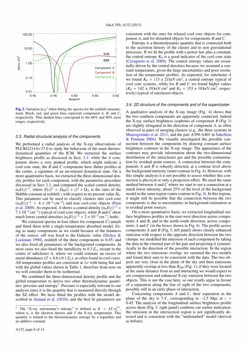
The redshift estimates we obtained from X-ray data for com-ponents A (z = 0.445± 0.006) and C (z = 0.46± 0.01) are nicelyconsistent with the spectroscopic values found in the SDSSarchive for their central brightest galaxies (0.450 and 0.452,respectively). Concerning component B, even without consid-ering the MOS1 detector, we still find a higher best fit value(z = 0.48 ± 0.01) with respect to the other two components.This is shown in Fig. 2, where we compare the variation of χ2

for the joint fits (see Table 2) of the three components. Whilecomponent A and C are consistent with being at the same red-shift at less than 1σ, component B is likely located at a higherredshift, although consistent at less than 2σ with the positionof the other clusters. Therefore, component B is likely sepa-rated along the line of sight from the two other components by69 (−30, +25) Mpc (150 Mpc, if we consider the redshift esti-mate obtained with the three detectors). While this large separa-tion suggests that the cluster B is not interacting with the othercomponents, it is still consistent with the three objects being partof the same supercluster structure (Bahcall 1999).

Using the best fit redshift estimates for the three components,we recomputed the physical parameters in Table 1. While thevariations for cluster A and C are negligible, for cluster B wefound YX = (0.74± 0.19)× 1014 M keV, M500 = (1.89± 0.20)×1014 M and R500 = (726 ± 25) kpc.

A132, page 5 of 14

A&A 550, A132 (2013)

Fig. 2. Variation in χ2 when fitting the spectra for the redshift measure-ment. Black, red, and green lines represent component A, B, and C,respectively. Thin dashed lines correspond to the 68% and 90% errorranges, respectively.

3.3. Radial structural analysis of the components

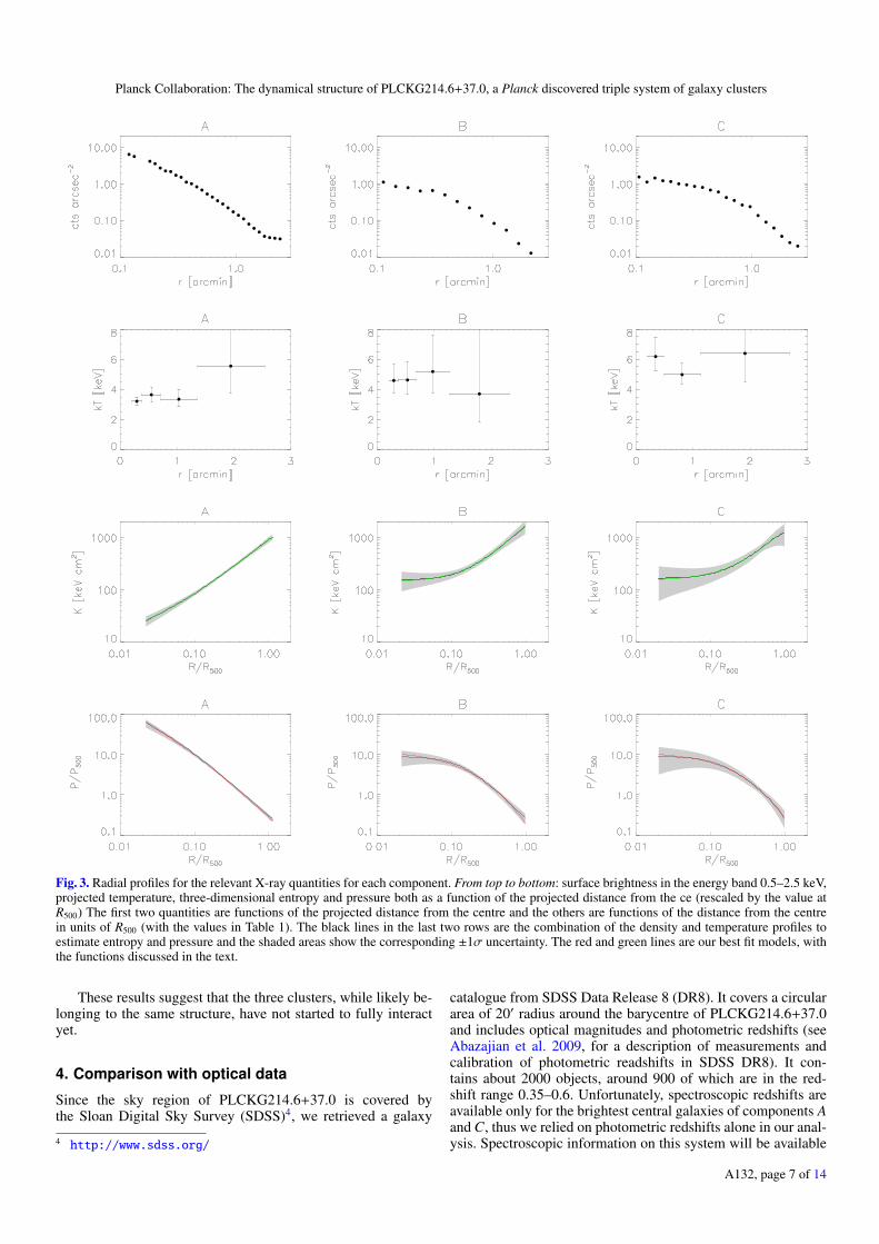
We performed a radial analysis of the X-ray observations ofPLCKG214.6+37.0 to study the behaviour of the main thermo-dynamical quantities of the ICM. We extracted the surfacebrightness profile as discussed in Sect. 3.1: while the A com-ponent shows a very peaked profile, which might indicate acool core state, the B and C components have flatter profiles atthe centre, a signature of an un-relaxed dynamical state. On amore quantitative basis, we extracted the three-dimensional den-sity profiles for each component, with the parametric procedurediscussed in Sect. 3.1, and computed the scaled central density,n0E(z)−2, where E(z)2 = ΩM(1 + z)3 + ΩΛ is the ratio of theHubble constant at redshift z with respect to its present value H0.This parameter can be used to classify clusters into cool-core(n0E(z)−2 > 4 × 10−2 cm−3) and non cool-core objects (Prattet al. 2009). As expected, A shows a central density (n0E(z)−2 =7× 10−2 cm−3) typical of cool-core objects, while B and C showmuch lower central densities (n0E(z)−2 = 2 × 10−3 cm−3, both).

We extracted spectra in four (three for component C) annuliand fitted them with a single-temperature absorbed model, fix-ing as many components as we could because of the faintnessof the source: nH was fixed to the Galactic value (Dickey &Lockman 1990), redshift of the three components to 0.45; andwe also fixed all parameters of the background components. Inmost cases we also fixed the metallicity to 0.3 Z, except in thecentre of subcluster A, where we could estimate an excess ofmetal abundance (Z = 0.6±0.1 Z), as often found in cool cores.All temperature profiles are consistent at 1σ with being flat andwith the global values shown in Table 1, therefore from now onwe will consider them to be isothermal.

We combined the three-dimensional density profile and theglobal temperature to derive two other thermodynamic quanti-ties: pressure and entropy3. Pressure is especially relevant to ouranalysis since it is the quantity that is measured directly throughthe SZ effect. We have fitted the profiles with the model de-scribed in Arnaud et al. (2010), and the best fit parameters are

3 The “X-ray astronomer’s entropy” is defined as K = kT/n2/3e ,

where ne is the electron density and T the X-ray temperature. Thisquantity is related to the thermodynamic entropy by a logarithm andan additive constant.

consistent with the ones for relaxed cool core objects for com-ponent A, and for disturbed objects for components B and C.

Entropy is a thermodynamic quantity that is connected bothto the accretion history of the cluster and to non gravitationalprocesses. If we fit the profile with a power law plus a constant,the central entropy K0 is a good indicator of the cool core state(Cavagnolo et al. 2009). The central entropy values are essen-tially driven by the central densities because we assumed a con-stant temperature, given the large uncertainties and poor resolu-tion of the temperature profiles. As expected, for subcluster Awe found K0 = (13 ± 2) keV cm2, a central entropy typical ofcool core systems, while for B and C we found higher values(K0 = 142 ± 10 keV cm2 and K0 = 153 ± 18 keV cm2, respec-tively) typical of unrelaxed objects.

3.4. 2D structure of the components and of the supercluster

A qualitative analysis of the X-ray image (Fig. 4) shows thatthe two southern components are apparently connected. Indeedthe X-ray surface brightness isophotes of component B (Fig. 1)are slightly elongated in the direction of component A, as oftenobserved in pairs of merging clusters (e.g., the three systems inMaurogordato et al. 2011; and the pair A399-A401 in Sakelliou& Ponman 2004). We visually investigated the possible con-nection between the components by drawing constant surfacebrightness contours in the X-ray image. The appearance of thecontours may provide information about the two-dimensionaldistribution of the intracluster gas and the possible contamina-tion by residual point sources. A connection between the com-ponents A and B is robustly detected, at a contour level abovethe background intensity (inner contour in Fig. 4). However, withthis simple analysis it is not possible to assess whether this con-nection is physical or only a projection effect. We used the samemethod between A and C where we start to see a connection at amuch lower intensity, about 25% of the level of the backgroundmodel in the same region (outer contour in Fig. 4). In this regime,it might still be possible that the connection between the twocomponents is due to uncertainties in background estimation orto residual point sources.

On a more quantitative basis, we extracted longitudinal sur-face brightness profiles in the east-west direction across compo-nents A and B, and in the north-south direction, across compo-nents A and C (in the boxes shown in Fig. 4). The profile acrosscomponents A and B (Fig. 5, left panel) shows clearly enhancedemission with respect to the opposite direction between the twoclumps: we modelled the emission of each component by takingthe data in the external part of the pair and projecting it symmet-rically in the direction of the possible interaction. In the regionwhere the two emissions overlap, we summed the two modelsand found their sum to be consistent with the data. The two ob-jects are very close in the plane of the sky and their emissionsapparently overlap at less than R500 (Fig. 1); if they were locatedat the same distance from us and interacting we would expect tosee compression and enhanced X-ray emission between the twoobjects. This is not the case here, so our results argue in favourof a separation along the line of sight of the two components,possibly still in an early phase of interaction.

Concerning components A and C, their separation in theplane of the sky is 7.4′, corresponding to ∼2.5 Mpc at z =0.45. The analysis of the longitudinal surface brightness profileacross them (Fig. 5, right panel) confirms our earlier indication:the emission in the intersection region is not significantly de-tected and is consistent with the “undisturbed” model (derivedas before).

A132, page 6 of 14

Planck Collaboration: The dynamical structure of PLCKG214.6+37.0, a Planck discovered triple system of galaxy clusters

Fig. 3. Radial profiles for the relevant X-ray quantities for each component. From top to bottom: surface brightness in the energy band 0.5–2.5 keV,projected temperature, three-dimensional entropy and pressure both as a function of the projected distance from the ce (rescaled by the value atR500) The first two quantities are functions of the projected distance from the centre and the others are functions of the distance from the centrein units of R500 (with the values in Table 1). The black lines in the last two rows are the combination of the density and temperature profiles toestimate entropy and pressure and the shaded areas show the corresponding ±1σ uncertainty. The red and green lines are our best fit models, withthe functions discussed in the text.

These results suggest that the three clusters, while likely be-longing to the same structure, have not started to fully interactyet.

4. Comparison with optical data

Since the sky region of PLCKG214.6+37.0 is covered bythe Sloan Digital Sky Survey (SDSS)4, we retrieved a galaxy

4 http://www.sdss.org/

catalogue from SDSS Data Release 8 (DR8). It covers a circulararea of 20′ radius around the barycentre of PLCKG214.6+37.0and includes optical magnitudes and photometric redshifts (seeAbazajian et al. 2009, for a description of measurements andcalibration of photometric readshifts in SDSS DR8). It con-tains about 2000 objects, around 900 of which are in the red-shift range 0.35–0.6. Unfortunately, spectroscopic redshifts areavailable only for the brightest central galaxies of components Aand C, thus we relied on photometric redshifts alone in our anal-ysis. Spectroscopic information on this system will be available

A132, page 7 of 14

A&A 550, A132 (2013)

Fig. 4. XMM-Newton wavelet filtered image of PLCKG214.6+37.0.Contours overlaid correspond to the levels where we start to see con-nection between the components. The green and yellow regions showwhere we extracted longitudinal profiles.

from our follow-up programme and will be discussed in a forth-coming paper.

4.1. Photometric redshifts of the three components

We used the archival photometric redshifts in our catalogue toestimate the redshift of the three components. We extracted asub-catalogue selecting only galaxies in the photometric red-shift range 0.35–0.6 and, for each clump, we calculated the me-dian redshift of the galaxy population around the X-ray centreas a function of the cutoff radius. The resulting plot is shown inFig. 6. Components A and C are both consistent with the spec-troscopic value of their central galaxies (z = 0.45), but the in-nermost 2′ of component B indicate a slightly higher redshift(zphot ' 0.47), similar to the results of the X-ray analysis, al-though consistent at 2σ with the values of the other components.At larger radii, the redshift estimates for the three clumps areall consistent with each other. It should be noted however thatcomponents A and B are separated only by '2 arcmin, thus allthe estimates at similar or larger radii may be contaminated bygalaxies belonging to the other cluster.

4.2. Optical appearance and morphology of the cluster

We used the catalogue from SDSS to build two-dimensionalgalaxy density maps in different photometric redshift cuts(Fig. 7), with a width ∆zphot = 0.04. We assigned the galax-ies to a fine grid of 24′′ per pixel, which is then degradedwith a Gaussian beam to an effective resolution of 3′. We alsocomputed a significance map using as reference ten random non-overlapping control regions in a 9 deg2 area around the system.

Clear galaxy overdensities show up around zphot = 0.46 at thelocation of the three X-ray clumps. However, these overdensitiesdo not appear isolated. At the location of cluster B, we see anoverpopulation of galaxies towards higher redshift (5σ peak atzphot ∼ 0.5), consistent with the redshift z = 0.48 we found inX-rays, whereas the overdensity extends towards slightly lowerredshifts (zphot ∼ 0.42) at the position of cluster A. There arealso indications of another concentration close to component Bat higher redshift (0.52–0.6).

We investigated the maps in Fig. 7 to look for a possiblepopulation of inter-cluster galaxies: i.e., objects not associatedwith one of the three clumps but rather with the whole struc-ture, which would support a scenario where the three clumps arephysically connected. We draw iso-contours levels in the sig-nificance map (Fig. 7): the outermost contour between 0.44 and0.52 connecting the three clumps indicates the presence of a 3σexcess in the galaxy number density above background in theinter-cluster region.

5. Comparison with Planck

5.1. Total SZ signal

As a simple comparison of the SZ and X-ray properties, we cancompare the Planck Y measurement with the predicted valuesfrom the sum of the YX estimates of all three components, usingthe scaling relations in Arnaud et al. (2010). From our X-rayestimates (Table 1), we predict the total integrated value of theComptonisation parameter within a sphere of radius 5 R500 forthe sum of the three components to be Yx,5 R500 = (7.52 ± 0.9) ×10−4 arcmin2. This is about 50% of the measured signal in thesame region which was found in Paper I and the two values arecompatible within 2.3σ.

In the following, we work under the assumption that the threeclusters are all located at the same redshift z = 0.45. Consideringthe best fit redshift for component B leads to a slightly smallerSZ flux Yx,5 R500 = (6.44 ± 0.7) × 10−4 arcmin2.

As discussed in Sect. 2.1, we used the parameters providedin Table 1 to improve our estimate of the total SZ signal of thisstructure from Planck data. We built a specific template from theX-ray analysis, made from three universal pressure profiles cutto 5 R500 (Arnaud et al. 2010) corresponding to the three compo-nents. Each component is placed at its precise coordinates andthe size is given by the R500 value in Table 1. We also fixedthe relative intensity between the components to verify A/C =0.96/1.61 and B/C = 1.22/1.61 for the ratio of integrated fluxes.Then we ran the MMF3 algorithm (Melin et al. 2006) to estimatethe amplitude of the template (and hence the total SZ signal ofthe whole system), and we found Y5 R500 = (12±3)×10−4 arcmin2,when centring the map on component B5. Our estimate of the su-percluster SZ flux is slightly larger than the X-ray prediction butconsistent at '1.3σ (1.8σ using z = 0.516 for component B).We further allowed the position of the template to be a free pa-rameter and found that the algorithm is able to reconstruct theposition of the peak with a positional accuracy of one sky pixel(1.7 × 1.7 arcmin2, in a HEALPIX projection of Nside = 2048,

5 The MMF3 algorithm estimates the noise (instrumental and astro-physical) in a region of 10 × 10 deg2 around the centre (excluding theregion within 5R500), therefore changing the centring from one compo-nent to the other can affect the background estimation and hence theflux and signal-to-noise ratio. Centring maps on component A we foundY5R500 = (10±3)×10−4 arcmin2 and on C Y5R500 = (13±3)×10−4 arcmin2.Our SZ flux estimations are all compatible with each other.

A132, page 8 of 14

Planck Collaboration: The dynamical structure of PLCKG214.6+37.0, a Planck discovered triple system of galaxy clusters

Fig. 5. X-ray Longitudinal profile in the east-west (left panel) and north-south directions (right panel). Left panel: negative distances correspond tocomponent B, positive ones to component A. The red and blue lines show the “undisturbed” models for components B and A (see text), respectively,while the green line in the intersection region is the sum of the two models. Right panel: negative distances correspond to component A, positiveones to component C. The red and blue lines show the “undisturbed” models for components A and C, respectively (see text).

Fig. 6. Median photometric redshifts for the three clumps (A black cir-cles; B red squares; C green diamonds) of all the galaxies within the cut-off radius. The error bars are the standard deviations of the photometricredshifts distributions. Given the small separation between componentsA and B, the points at radii &2′ may be contaminated by galaxies of theother structure.

Górski et al. 2005). This is consistent with the positional ac-curacy of the MMF3 algorithm, which has been tested both onsimulations and on real data with known clusters.

The discrepancy between the observed SZ signal and the pre-diction from the YX measurement is decreased with respect toPaper I: while the X-ray prediction was only 40% of the SZ mea-surement, it is now between 60 and 77%, depending on the mapcentring. This is partly due to the higher YX values we found inthis analysis with respect to Paper I, especially for componentsB and C. It is also certainly due to the improved accuracy of theHFI maps obtained with two full surveys of the sky and to themulti-component model we have used to estimate the SZ flux,with respect to the data from the first sky survey and to the sin-gle component model that was used in Paper I. Indeed, theseresults confirm our capability to extract faint SZ signals, whenguided by X-ray priors (Planck Collaboration 2011e).

5.2. SZ signal distribution

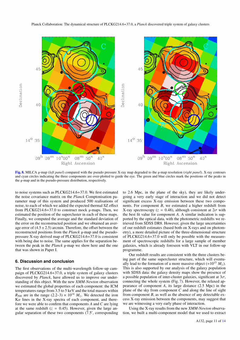
It is possible to combine the X-ray images with the temperaturesof the components to predict the distribution of the SZ signal(see Mroczkowski et al. 2012, for a similar approach). X-rayimages in the soft band are proportional to the square of thedensity integrated along the line of sight and therefore theirsquare root can be combined with a temperature map to derivea pseudo-pressure map6, which when smoothed with the Planckresolution, can be qualitatively compared with the y-maps. Wecombined the background-subtracted X-ray image with a tem-perature map, built assuming the mean temperature value in eachcomponent (Table 1) within R500 and zero outside, to producea pseudo-pressure map, that we smoothed with a Gaussian fil-ter of 10′ FWHM to mimic the resolution of Planck y-maps.Planck cannot spatially resolve the three components of this ob-ject, therefore we expect the peak of the pseudo-pressure map tobe located around the barycentre of the system, just because ofresolution effects. The results are shown in Fig. 8, compared withthe MILCA y-map. The position of the peak in the SZ map doesnot coincide with the peak of the pseudo pressure map: while thelatter is located as expected at the barycentre between the threecomponents, the y-map suggests an excess of pressure to the SWof component A. The offset between the two peaks is '5′.

We have performed some tests both on the X-ray and onthe SZ maps to investigate the origin of this offset. On theX-ray side, we have produced surface brightness images us-ing a different background modelling. The first test concernsthe background subtraction: we used the ESAS software7 toproduce particle background and residual soft proton imagesand we created images of the “sky background” components(CXB and Galactic foregrounds), modelling them in an exter-nal annulus (Leccardi & Molendi 2008) and rescaling themacross the field of view (Ettori et al. 2010). Point sources couldalso affect the position of the pseudo pressure peak, therefore

6 Although deriving pseudo-pressure maps as discussed in the text iscustomary in the literature, we underline here that this approach is notcompletely valid. The X-ray surface brightness, ignoring the tempera-ture dependance, is proportional to

∫n2dl and its square root is never

equal to∫

ndl, which is the expression that should enter in the defi-nition of the Comptonisation parameter y. However, pseudo-pressuremaps can still be used for qualitative comparison with the y-maps.7 http://heasarc.nasa.gov/docs/xmm/xmmhp_xmmesas.html

A132, page 9 of 14

A&A 550, A132 (2013)

Fig. 7. Galaxy density maps for cluster members in the SDSS catalogue (colours) in different photometric redshift cuts: 0.40–0.44 (upper left);0.44–0.48 (upper right); 0.48–0.52 (lower left); and 0.52–0.56 (lower right). The cyan contours overlaid mark the significance of each densitypeak at 3, 4, and 5σ, respectively. The black contours show the X-ray distribution and the red circles and letters mark the three components.

we ran a different point source algorithm using the SAS taskedetect_chain on MOS and pn images in five energy bands,and we added undetected sources we identified with a visualinspection of the images. Both these tests showed a negligi-ble impact on the position of the peak, which in fact is lo-cated where it is expected to be, at the barycentre of the threecomponents.

For the SZ effect, we have compared the maps reconstructedwith different ILC-based algorithms. Besides MILCA, we testedGMCA (Bobin et al. 2008) and NILC (Delabrouille et al. 2009)algorithms (see Planck Collaboration 2013, for a summary de-scription and a comparison at the cluster scale of the three

methods). The three y-maps are very consistent and the positionof the peak does not change across the maps.

We also compared y-maps obtained with different releasesof the data finding '5′ discrepancies in the position of the peak,comparable to the offset between the X-ray and y-maps peaks,discussed above. Indeed the y-map presented in Paper I showeda qualitative agreement with X-ray contours. We performed ded-icated Monte Carlo simulations to estimate the expected er-ror in the reconstruction of the position of PLCKG214.6+37.0.The presence of correlated noise in the y-map produced fromPlanck data can be a major source of error in reconstructingthe position of clusters, in particular in the case of low signal

A132, page 10 of 14

Planck Collaboration: The dynamical structure of PLCKG214.6+37.0, a Planck discovered triple system of galaxy clusters

Fig. 8. MILCA y-map (left panel) compared with the pseudo pressure X-ray map degraded to the y-map resolution (right panel). X-ray contoursand cyan circles indicating the three components are over-plotted to guide the eye. The green and blue circles mark the positions of the peaks inthe y-map and in the pseudo-pressure distribution, respectively.

to noise systems such as PLCKG214.6+37.0. We first estimatedthe noise covariance matrix on the Planck Comptonisation pa-rameter map of this system and produced 500 realisations ofnoise, to each of which we added the expected thermal SZ effectfrom PLCKG214.6+37.0 to construct mock y-maps. Then, weestimated the position of the supercluster in each of these maps.Finally, we computed the average and the standard deviation ofthe error on the reconstructed position and we obtained an aver-age error of (4.5± 2.5) arcmin. Therefore, the offset between thereconstructed positions from the Planck y-map and the pseudo-pressure X-ray derived map of PLCKG214.6+37.0 is consistentwith being due to noise. The same applies for the separation be-tween the peak in the Planck y-map we show here and the onethat was shown in Paper I.

6. Discussion and conclusion

The first observations of the multi-wavelength follow-up cam-paign of PLCKG214.6+37.0, a triple system of galaxy clustersdiscovered by Planck, have allowed us to improve our under-standing of this object. With the new XMM-Newton observationwe estimated the global properties of each component: the ICMtemperatures range from 3.5 to 5 keV and the total masses withinR500 are in the range (2.2–3) × 1014 M. We detected the ironKα lines in the X-ray spectra of each component, and there-fore we were able to confirm that components A and C are lyingat the same redshift (z = 0.45). However, given the large an-gular separation of these two components (7.5′, corresponding

to 2.6 Mpc, in the plane of the sky), they are likely under-going a very early stage of interaction and we did not detectsignificant excess X-ray emission between these two compo-nents. For component B, we estimated a higher redshift fromX-ray spectroscopy (z = 0.48), although consistent at 2σ withthe best fit value for component A. A similar indication is sup-ported by the optical data, with the photometric redshifts we re-trieved from SDSS DR8. However, given the large uncertaintiesof our redshift estimates (based both on X-rays and on photom-etry), a more detailed picture of the three-dimensional structureof PLCKG214.6+37.0 will only be possible with the measure-ment of spectroscopic redshifts for a large sample of membergalaxies, which is already foreseen with VLT in our follow-upprogramme.

Our redshift results are consistent with the three clusters be-ing part of the same supercluster structure, which will eventu-ally lead to the formation of a more massive object ('1015 M).This is also supported by our analysis of the galaxy populationwith SDSS data: the galaxy density maps show the presence ofa possible population of inter-cluster galaxies, significant at 3σ,connecting the whole system (Fig. 7). However, the relaxed ap-pearance of component A, its large distance (2.5 Mpc) in theplane of the sky from component C and along the line of sightfrom component B, as well as the absence of any detectable ex-cess X-ray emission between the components, may suggest thatwe are witnessing a very early phase of interaction.

Using the X-ray results from the new XMM-Newton observa-tion, we built a multi-component model that we used to extract

A132, page 11 of 14

A&A 550, A132 (2013)

the total SZ signal from Planck data. We compared the improvedestimate of YSZ with the prediction from X-rays and we found thelatter to be about 68% of the measured SZ signal. The discrep-ancy between these two values is reduced with respect to Paper Iand is not at the 1.2σ level.

The results from our simulations have shown that an off-set as large as 5′ can be expected in the reconstructed y-mapsfor low-significance objects, due to noise fluctuations and as-trophysical contributions. With this study we have illustratedthe expected difficulty of accurately reconstructing the two-dimensional SZ signal for objects with low signal-to-noise ra-tio. Indeed the instrumental noise and astrophysical contamina-tion compete with the SZ effect at the detection limit thresh-old. Nonetheless, objects like PLCKG214.6+37.0 can be de-tected with a dedicated optimal filtering detection method, andthe SZ signal can be reconstructed assuming priors (such as po-sition, size, and relative intensity) from other wavelengths.

Despite a deep re-observation of this system withXMM-Newton, the intrinsic limitations of our X-ray data and ofthe current Planck SZ maps do not allow us, for the time beingto assess the presence of possible inter-cluster emission.

A careful analysis of the galaxy dynamics in the complexpotential of this object and of the mass distribution from weaklensing will both be available with our on-going optical followup programme. These observations, combined with the resultspresented in this paper and with new Planck data obtained intwo other full surveys of the sky, might lead to a deeper under-standing of this triple system.

Acknowledgements. A description of the Planck Collaboration and a list ofits members, indicating which technical or scientific activities they havebeen involved in, can be found at http://www.rssd.esa.int/Planck.The Planck Collaboration acknowledges the support of: ESA; CNES andCNRS/INSU-IN2P3-INP (France); ASI, CNR, and INAF (Italy); NASA andDoE (USA); STFC and UKSA (UK); CSIC, MICINN, and JA (Spain); Tekes,AoF, and CSC (Finland); DLR and MPG (Germany); CSA (Canada); DTUSpace (Denmark); SER/SSO (Switzerland); RCN (Norway); SFI (Ireland);FCT/MCTES (Portugal); and DEISA (EU). The present paper is also partlybased on observations obtained with XMM-Newton, an ESA science missionwith instruments and contributions directly funded by ESA Member States andthe USA (NASA), and on data retrieved from SDSS-III. Funding for SDSS-III has been provided by the Alfred P. Sloan Foundation, the ParticipatingInstitutions, the National Science Foundation, and the U.S. Department ofEnergy Office of Science. The SDSS-III web site is http://www.sdss3.org/.

ReferencesAbazajian, K. N., Adelman-McCarthy, J. K., Agüeros, M. A., et al. 2009, ApJS,

182, 543Arnaud, M., Pratt, G. W., Piffaretti, R., et al. 2010, A&A, 517, A92Bahcall, N. A. 1999, in Formation of Structure in the Universe, 135Balucinska-Church, M., & McCammon, D. 1992, ApJ, 400, 699Bardelli, S., Zucca, E., Zamorani, G., Vettolani, G., & Scaramella, R. 1998,

MNRAS, 296, 599Bersanelli, M., Mandolesi, N., Butler, R. C., et al. 2010, A&A, 520, A4Bobin, J., Moudden, Y., Starck, J.-L., Fadili, J., & Aghanim, N. 2008, Stat.

Methodol., 5, 307Bourdin, H., & Mazzotta, P. 2008, A&A, 479, 307Bourdin, H., Arnaud, M., Mazzotta, P., et al. 2011, A&A, 527, A21Cavagnolo, K. W., Donahue, M., Voit, G. M., & Sun, M. 2009, ApJS, 182, 12De Luca, A., & Molendi, S. 2004, A&A, 419, 837Delabrouille, J., Cardoso, J.-F., Le Jeune, M., et al. 2009, A&A, 493, 835Dickey, J. M., & Lockman, F. J. 1990, ARA&A, 28, 215Eriksen, H. K., Banday, A. J., Górski, K. M., & Lilje, P. B. 2004, ApJ, 612, 633Ettori, S., Gastaldello, F., Leccardi, A., et al. 2010, A&A, 524, A68Giacintucci, S., Venturi, T., Brunetti, G., et al. 2005, A&A, 440, 867Górski, K. M., Hivon, E., Banday, A. J., et al. 2005, ApJ, 622, 759Grevesse, N., & Sauval, A. J. 1998, Space Sci. Rev., 85, 161Hurier, G., Hildebrandt, S. R., & Macias-Perez, J. F. 2010 [arXiv:1007.1149]Kravtsov, A. V., Vikhlinin, A., & Nagai, D. 2006, ApJ, 650, 128Kull, A., & Böhringer, H. 1999, A&A, 341, 23

Kuntz, K. D., & Snowden, S. L. 2000, ApJ, 543, 195Kuntz, K. D., & Snowden, S. L. 2008, A&A, 478, 575Lamarre, J., Puget, J., Ade, P. A. R., et al. 2010, A&A, 520, A9Leahy, J. P., Bersanelli, M., D’Arcangelo, O., et al. 2010, A&A, 520, A8Leccardi, A., & Molendi, S. 2008, A&A, 487, 461Liivamägi, L. J., Tempel, E., & Saar, E. 2012, A&A, 539, A80Lumb, D. H., Warwick, R. S., Page, M., & De Luca, A. 2002, A&A, 389, 93Mandolesi, N., Bersanelli, M., Butler, R. C., et al. 2010, A&A, 520, A3Maurogordato, S., Sauvageot, J. L., Bourdin, H., et al. 2011, A&A, 525, A79Melin, J., Bartlett, J. G., & Delabrouille, J. 2006, A&A, 459, 341Menanteau, F., Hughes, J. P., Sifon, C., et al. 2012, ApJ, 748, 7Mennella A., Butter, R. C., Curto, A., et al. 2011, A&A, 536, A3Mroczkowski, T., Dicker, S., Sayers, J., et al. 2012, ApJ, 761, 47Planck Collaboration 2011a, A&A, 536, A1Planck Collaboration 2011b, A&A, 536, A2Planck Collaboration 2011c, A&A, 536, A9Planck Collaboration 2011d, A&A, 536, A8Planck Collaboration 2011e, A&A, 536, A10Planck Collaboration 2011f, A&A, 536, A26Planck Collaboration 2013, A&A, 550, A131Planck HFI Core Team 2011a, A&A, 536, A4Planck HFI Core Team 2011b, A&A, 536, A6Pratt, G. W., Croston, J. H., Arnaud, M., & Böhringer, H. 2009, A&A, 498, 361Rosset, C., Tristram, M., Ponthieu, N., et al. 2010, A&A, 520, A13Rossetti, M., Ghizzardi, S., Molendi, S., & Finoguenov, A. 2007, A&A, 463,

839Sakelliou, I., & Ponman, T. J. 2004, MNRAS, 351, 1439Slezak, E., Durret, F., & Gerbal, D. 1994, AJ, 108, 1996Smith, R. K., Brickhouse, N. S., Liedahl, D. A., & Raymond, J. C. 2001, ApJ,

556, L91Starck, J.-L., & Pierre, M. 1998, in Astronomical Data Analysis Software and

Systems VII, eds. R. Albrecht, R. N. Hook, & H. A. Bushouse, ASP Conf.Ser., 145, 500

Starck, J. L., Fadili, J., & Murtagh, F. 2007, IEEE Trans. Image Process., 16Sunyaev, R. A., & Zeldovich, Y. B. 1972, Comm. Astrophys. Space Phys., 4,

173Tauber, J. A., Mandolesi, N., Puget, J., et al. 2010, A&A, 520, A1Vikhlinin, A., Forman, W., & Jones, C. 1997, ApJ, 474, L7Vikhlinin, A., Kravtsov, A., Forman, W., et al. 2006, ApJ, 640, 691Zacchei, A., Maino, D., Baccigalupi, C. A., et al. 2011, A&A, 536, A5Zhang, B., Fadili, J., & Starck, J. L. 2008, IEEE Trans. Image Process., 17

1 APC, AstroParticule et Cosmologie, Université Paris Diderot,CNRS/IN2P3, CEA/lrfu, Observatoire de Paris, Sorbonne ParisCité, 10 rue Alice Domon et Léonie Duquet, 75205 Paris Cedex 13,France

2 Aalto University Metsähovi Radio Observatory, Metsähovintie 114,02540 Kylmälä, Finland

3 Academy of Sciences of Tatarstan, Bauman Str., 20, 420111 Kazan,Republic of Tatarstan, Russia

4 African Institute for Mathematical Sciences, 6-8 Melrose Road,Muizenberg, Cape Town, South Africa

5 Agenzia Spaziale Italiana Science Data Center, c/o ESRIN, viaGalileo Galilei, Frascati, Italy

6 Agenzia Spaziale Italiana, Viale Liegi 26, Roma, Italy7 Astrophysics Group, Cavendish Laboratory, University of

Cambridge, J J Thomson Avenue, Cambridge CB3 0HE, UK8 Atacama Large Millimeter/submillimeter Array, ALMA Santiago

Central Offices, Alonso de Cordova 3107, Vitacura, 763 0355Casilla, Santiago, Chile

9 CITA, University of Toronto, 60 St. George St., TorontoON M5S 3H8, Canada

10 CNRS, IRAP, 9 Av. Colonel Roche, BP 44346, 31028 ToulouseCedex 4, France

11 California Institute of Technology, Pasadena, California, USA12 Centre of Mathematics for Applications, University of Oslo,

Blindern, Oslo, Norway13 Centro de Astrofísica, Universidade do Porto, Rua das Estrelas,

4150-762 Porto, Portugal14 Centro de Estudios de Física del Cosmos de Aragón (CEFCA),

Plaza San Juan, 1, planta 2, 44001 Teruel, Spain15 Computational Cosmology Center, Lawrence Berkeley National

Laboratory, Berkeley, California, USA

A132, page 12 of 14

Planck Collaboration: The dynamical structure of PLCKG214.6+37.0, a Planck discovered triple system of galaxy clusters

16 Consejo Superior de Investigaciones Científicas (CSIC), Madrid,Spain

17 DSM/Irfu/SPP, CEA-Saclay, 91191 Gif-sur-Yvette Cedex, France18 DTU Space, National Space Institute, Technical University of

Denmark, Elektrovej 327, 2800 Kgs. Lyngby, Denmark19 Département de Physique Théorique, Université de Genève, 24 Quai

E. Ansermet, 1211 Genève 4, Switzerland20 Departamento de Física Fundamental, Facultad de Ciencias,

Universidad de Salamanca, 37008 Salamanca, Spain21 Departamento de Física, Universidad de Oviedo, Avda. Calvo Sotelo

s/n, Oviedo, Spain22 Department of Astronomy and Geodesy, Kazan Federal University,

Kremlevskaya Str., 18, 420008 Kazan, Russia23 Department of Astrophysics/IMAPP, Radboud University

Nijmegen, PO Box 9010, 6500 GL Nijmegen, The Netherlands24 Department of Physics & Astronomy, University of British

Columbia, 6224 Agricultural Road, Vancouver, British Columbia,Canada

25 Department of Physics and Astronomy, Dana and David DornsifeCollege of Letter, Arts and Sciences, University of SouthernCalifornia, Los Angeles, CA 90089, USA

26 Department of Physics, Gustaf Hällströmin katu 2a, University ofHelsinki, Helsinki, Finland

27 Department of Physics, Princeton University, Princeton, New Jersey,USA

28 Department of Physics, University of California, Berkeley,California, USA

29 Department of Physics, University of California, One ShieldsAvenue, Davis, California, USA

30 Department of Physics, University of California, Santa Barbara,California, USA

31 Department of Physics, University of Illinois at Urbana-Champaign,1110 West Green Street, Urbana, Illinois, USA

32 Department of Statistics, Purdue University, 250 N. UniversityStreet, West Lafayette, Indiana, USA

33 Dipartimento di Fisica e Astronomia G. Galilei, Università degliStudi di Padova, via Marzolo 8, 35131 Padova, Italy

34 Dipartimento di Fisica e Scienze della Terra, Università di Ferrara,via Saragat 1, 44122 Ferrara, Italy

35 Dipartimento di Fisica, Università La Sapienza, P. le A. Moro 2,Roma, Italy

36 Dipartimento di Fisica, Università degli Studi di Milano, via Celoria,16 Milano, Italy

37 Dipartimento di Fisica, Università degli Studi di Trieste, via A.Valerio 2, Trieste, Italy

38 Dipartimento di Fisica, Università di Roma Tor Vergata, via dellaRicerca Scientifica, 1, Roma, Italy

39 Dipartimento di Matematica, Università di Roma Tor Vergata, viadella Ricerca Scientifica, 1, Roma, Italy

40 Discovery Center, Niels Bohr Institute, Blegdamsvej 17,Copenhagen, Denmark

41 Dpto. Astrofísica, Universidad de La Laguna (ULL), 38206La Laguna, Tenerife, Spain

42 European Southern Observatory, ESO Vitacura, Alonso de Cordova3107, Vitacura, 19001 Casilla, Santiago, Chile

43 European Space Agency, ESAC, Planck Science Office, Caminobajo del Castillo, s/n, Urbanización Villafranca del Castillo,Villanueva de la Cañada, Madrid, Spain

44 European Space Agency, ESTEC, Keplerlaan 1, 2201AZ Noordwijk, The Netherlands

45 GEPI, Observatoire de Paris, Section de Meudon, 5 place J. Janssen,92195 Meudon Cedex, France

46 Helsinki Institute of Physics, Gustaf Hällströmin katu 2, Universityof Helsinki, Helsinki, Finland

47 INAF – Osservatorio Astronomico di Padova, Vicolodell’Osservatorio 5, Padova, Italy

48 INAF – Osservatorio Astronomico di Roma, via di Frascati 33,Monte Porzio Catone, Italy

49 INAF – Osservatorio Astronomico di Trieste, via G.B. Tiepolo 11,Trieste, Italy

50 INAF Istituto di Radioastronomia, via P. Gobetti 101, 40129Bologna, Italy

51 INAF/IASF Bologna, via Gobetti 101, Bologna, Italy52 INAF/IASF Milano, via E. Bassini 15, Milano, Italy53 INFN, Sezione di Roma 1, Universit‘a di Roma Sapienza, Piazzale

Aldo Moro 2, 00185 Roma, Italy54 IPAG: Institut de Planétologie et d’Astrophysique de Grenoble,

Université Joseph Fourier, Grenoble 1/CNRS-INSU, UMR 5274,38041 Grenoble, France

55 IUCAA, Post Bag 4, Ganeshkhind, Pune University Campus, Pune411 007, India

56 Imperial College London, Astrophysics group, Blackett Laboratory,Prince Consort Road, London, SW7 2AZ, UK

57 Infrared Processing and Analysis Center, California Institute ofTechnology, Pasadena, CA 91125, USA

58 Institut Néel, CNRS, Université Joseph Fourier Grenoble I, 25 ruedes Martyrs, Grenoble, France

59 Institut Universitaire de France, 103, bd Saint-Michel, 75005, Paris,France

60 Institut d’Astrophysique Spatiale, CNRS (UMR 8617), UniversitéParis-Sud 11, Bâtiment 121, Orsay, France

61 Institut d’Astrophysique de Paris, CNRS (UMR 7095), 98bis boule-vard Arago, 75014, Paris, France

62 Institute for Space Sciences, Bucharest-Magurale, Romania63 Institute of Astro and Particle Physics, Technikerstrasse 25/8,

University of Innsbruck, 6020, Innsbruck, Austria64 Institute of Astronomy and Astrophysics, Academia Sinica, Taipei,

Taiwan65 Institute of Astronomy, University of Cambridge, Madingley Road,

Cambridge CB3 0HA, UK66 Institute of Theoretical Astrophysics, University of Oslo, Blindern,

Oslo, Norway67 Instituto de Astrofísica de Canarias, C/Vía Láctea s/n, La Laguna,

Tenerife, Spain68 Instituto de Física de Cantabria (CSIC-Universidad de Cantabria),

Avda. de los Castros s/n, Santander, Spain69 Jet Propulsion Laboratory, California Institute of Technology, 4800

Oak Grove Drive, Pasadena, California, USA70 Jodrell Bank Centre for Astrophysics, Alan Turing Building, School

of Physics and Astronomy, The University of Manchester, OxfordRoad, Manchester, M13 9PL, UK

71 Kapteyn Astronomical Institute, University of Groningen,Landleven 12, 9747 AD Groningen, The Netherlands

72 Kavli Institute for Cosmology Cambridge, Madingley Road,Cambridge, CB3 0HA, UK

73 LAL, Université Paris-Sud, CNRS/IN2P3, Orsay, France74 LERMA, CNRS, Observatoire de Paris, 61 avenue de

l’Observatoire, Paris, France75 Laboratoire AIM, IRFU/Service d’Astrophysique – CEA/DSM –

CNRS – Université Paris Diderot, Bât. 709, CEA-Saclay, 91191 Gif-sur-Yvette Cedex, France

76 Laboratoire Traitement et Communication de l’Information, CNRS(UMR 5141) and Télécom ParisTech, 46 rue Barrault, 75634 ParisCedex 13, France

77 Laboratoire de Physique Subatomique et de Cosmologie, UniversitéJoseph Fourier Grenoble I, CNRS/IN2P3, Institut NationalPolytechnique de Grenoble, 53 rue des Martyrs, 38026 GrenobleCedex, France

78 Laboratoire de Physique Théorique, Université Paris-Sud 11 &CNRS, Bâtiment 210, 91405 Orsay, France

79 Lawrence Berkeley National Laboratory, Berkeley, California, USA80 Max-Planck-Institut für Astrophysik, Karl-Schwarzschild-Str. 1,

85741 Garching, Germany81 Max-Planck-Institut für Extraterrestrische Physik,

Giessenbachstraße, 85748 Garching, Germany82 MilliLab, VTT Technical Research Centre of Finland, Tietotie 3,

Espoo, Finland83 National University of Ireland, Department of Experimental

Physics, Maynooth, Co. Kildare, Ireland84 Niels Bohr Institute, Blegdamsvej 17, Copenhagen, Denmark

A132, page 13 of 14

A&A 550, A132 (2013)

85 Observational Cosmology, Mail Stop 367-17, California Institute ofTechnology, Pasadena, CA, 91125, USA

86 Optical Science Laboratory, University College London, GowerStreet, London, UK

87 SISSA, Astrophysics Sector, via Bonomea 265, 34136 Trieste, Italy88 School of Physics and Astronomy, Cardiff University, Queens

Buildings, The Parade, Cardiff, CF24 3AA, UK89 Space Research Institute (IKI), Profsoyuznaya 84/32, Moscow,

Russia90 Space Research Institute (IKI), Russian Academy of Sciences,

Profsoyuznaya Str, 84/32, 117997 Moscow, Russia91 Space Sciences Laboratory, University of California, Berkeley,

California, USA92 Stanford University, Dept of Physics, Varian Physics Bldg, 382 via

Pueblo Mall, Stanford, California, USA

93 TÜBITAK National Observatory, Akdeniz University Campus,07058, Antalya, Turkey

94 Tuorla Observatory, Department of Physics and Astronomy,University of Turku, Väisäläntie 20, 21500 Piikkiö, Finland

95 UPMC Univ Paris 06, UMR7095, 98bis boulevard Arago, 75014,Paris, France

96 Université Denis Diderot (Paris 7), 75205 Paris Cedex 13, France97 Université de Toulouse, UPS-OMP, IRAP, 31028 Toulouse Cedex 4,

France98 University Observatory, Ludwig Maximilian University of Munich,

Scheinerstrasse 1, 81679 Munich, Germany99 University of Granada, Departamento de Física Teórica y del

Cosmos, Facultad de Ciencias, Granada, Spain100 Warsaw University Observatory, Aleje Ujazdowskie 4, 00-478

Warszawa, Poland

A132, page 14 of 14