photovoltaic (pv) type solar generators and their effect …
TRANSCRIPT
PHOTOVOLTAIC (PV) TYPE SOLAR GENERATORS AND THEIR EFFECT ON
DISTRIBUTION SYSTEMS
A Thesisin
Electrical Engineering
Presented to the Faculty of the Universityof Missouri–Kansas City in partial fulfillment of
the requirements for the degree
MASTER OF SCIENCE
byABDULSALAM ELSAIDI
B.Sc. , Al-Tahadi University, Sirte, Libya, 1999
Kansas City, Missouri2013

c© 2013
ABDULSALAM ELSAIDI
ALL RIGHTS RESERVED
PHOTOVOLTAIC (PV) TYPE SOLAR GENERATORS AND THEIR EFFECT ON
DISTRIBUTION SYSTEMS
Abdulsalam Elsaidi, Candidate for the Master of Science Degree
University of Missouri–Kansas City, 2013
ABSTRACT
Distribution systems are designed to operate in radial mode (the simplest system
topology) without any generation on the system, unidirectional power flow from the dis-
tribution substation to the customers via main feeder(s) and its(their) laterals within a
specified range of operating points. The rapid growth of PV module installations on the
distribution systems could not only offset the load but also cause a significant impact on
the flow of power (active and reactive), voltage level, and fault currents, therefore; con-
cerns about their potential impacts on the stability and operation of the power system have
become one of the important issues and may create barriers to their future expansion. The
most likely potential impact of the high PV penetration level is losing the voltage regula-
tion, because it is directly related to the amount of reverse power flow. The main goal of
this thesis is to approximate the maximum level of PV penetration which the system can
accommodate without any impact on the voltage profile, stability, and operation.
iii

APPROVAL PAGE
The faculty listed below, appointed by the Dean of the School of Computing and Engi-
neering, have examined a thesis titled “Photovoltaic (PV) Type Solar Generators and their
effect on distribution systems,” presented by Abdulsalam Elsaidi, candidate for the Master
of Science degree, and hereby certify that in their opinion it is worthy of acceptance.
Supervisory Committee
Ghulam M. Chaudhry, Ph.D., Committee ChairDepartment of Computer Science & Electrical Engineering
Cory Beard, Ph.D.Department of Computer Science & Electrical Engineering
Masud H. Chowdhury, Ph.D.Department of Computer Science & Electrical Engineering
Soundrapandian Sankar, Ph.D.Black & Veatch
Adjunct Instructor in Department of Computer Science & Electrical Engineering
iv
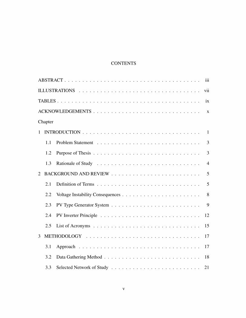
CONTENTS
ABSTRACT . . . . . . . . . . . . . . . . . . . . . . . . . . . . . . . . . . . . . . iii
ILLUSTRATIONS . . . . . . . . . . . . . . . . . . . . . . . . . . . . . . . . . . vii
TABLES . . . . . . . . . . . . . . . . . . . . . . . . . . . . . . . . . . . . . . . . ix
ACKNOWLEDGEMENTS . . . . . . . . . . . . . . . . . . . . . . . . . . . . . . x
Chapter
1 INTRODUCTION . . . . . . . . . . . . . . . . . . . . . . . . . . . . . . . . . 1
1.1 Problem Statement . . . . . . . . . . . . . . . . . . . . . . . . . . . . . 3
1.2 Purpose of Thesis . . . . . . . . . . . . . . . . . . . . . . . . . . . . . . 3
1.3 Rationale of Study . . . . . . . . . . . . . . . . . . . . . . . . . . . . . 4
2 BACKGROUND AND REVIEW . . . . . . . . . . . . . . . . . . . . . . . . . 5
2.1 Definition of Terms . . . . . . . . . . . . . . . . . . . . . . . . . . . . . 5
2.2 Voltage Instability Consequences . . . . . . . . . . . . . . . . . . . . . . 8
2.3 PV Type Generator System . . . . . . . . . . . . . . . . . . . . . . . . . 9
2.4 PV Inverter Principle . . . . . . . . . . . . . . . . . . . . . . . . . . . . 12
2.5 List of Acronyms . . . . . . . . . . . . . . . . . . . . . . . . . . . . . . 15
3 METHODOLOGY . . . . . . . . . . . . . . . . . . . . . . . . . . . . . . . . 17
3.1 Approach . . . . . . . . . . . . . . . . . . . . . . . . . . . . . . . . . . 17
3.2 Data Gathering Method . . . . . . . . . . . . . . . . . . . . . . . . . . . 18
3.3 Selected Network of Study . . . . . . . . . . . . . . . . . . . . . . . . . 21
v
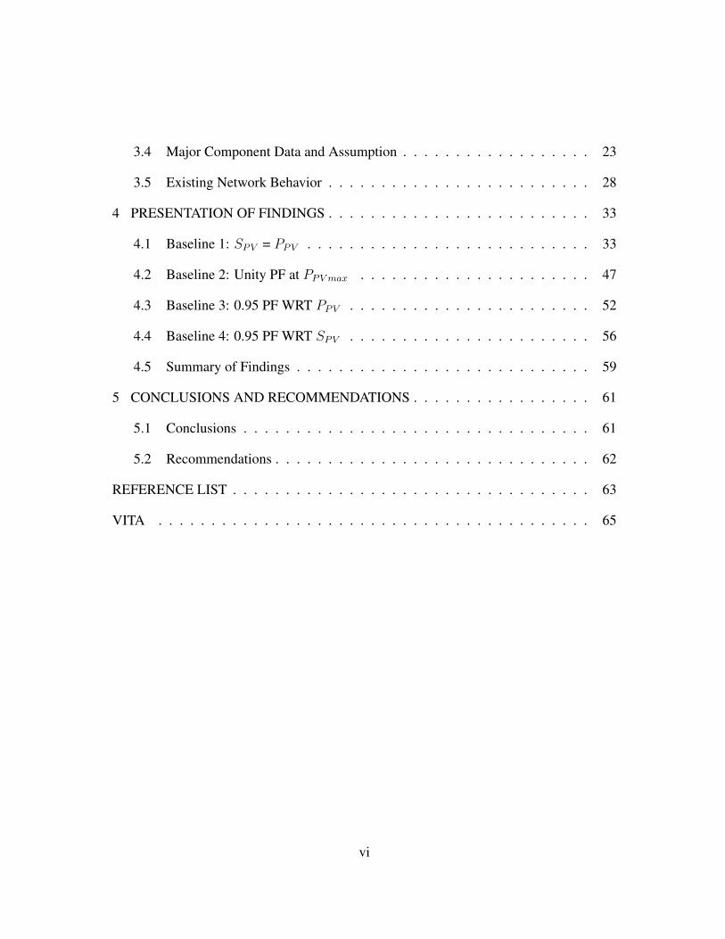
3.4 Major Component Data and Assumption . . . . . . . . . . . . . . . . . . 23
3.5 Existing Network Behavior . . . . . . . . . . . . . . . . . . . . . . . . . 28
4 PRESENTATION OF FINDINGS . . . . . . . . . . . . . . . . . . . . . . . . . 33
4.1 Baseline 1: SPV = PPV . . . . . . . . . . . . . . . . . . . . . . . . . . . 33
4.2 Baseline 2: Unity PF at PPVmax . . . . . . . . . . . . . . . . . . . . . . 47
4.3 Baseline 3: 0.95 PF WRT PPV . . . . . . . . . . . . . . . . . . . . . . . 52
4.4 Baseline 4: 0.95 PF WRT SPV . . . . . . . . . . . . . . . . . . . . . . . 56
4.5 Summary of Findings . . . . . . . . . . . . . . . . . . . . . . . . . . . . 59
5 CONCLUSIONS AND RECOMMENDATIONS . . . . . . . . . . . . . . . . . 61
5.1 Conclusions . . . . . . . . . . . . . . . . . . . . . . . . . . . . . . . . . 61
5.2 Recommendations . . . . . . . . . . . . . . . . . . . . . . . . . . . . . . 62
REFERENCE LIST . . . . . . . . . . . . . . . . . . . . . . . . . . . . . . . . . . 63
VITA . . . . . . . . . . . . . . . . . . . . . . . . . . . . . . . . . . . . . . . . . 65
vi
ILLUSTRATIONS
Figure Page
1 U.S. PV Installation Forecast, 2010-2016E . . . . . . . . . . . . . . . . . 1
2 AC Power Relationships . . . . . . . . . . . . . . . . . . . . . . . . . . 6
3 The process of the PV system (Courtesy of “www.TheSolarPlanner.com”) 10
4 A residential grid-connected PV system (Courtesy of “en.Wikipedia.org”) 11
5 An inverter’s reactive power limits . . . . . . . . . . . . . . . . . . . . . 13
6 Relationship between inverter size and its reactive power capability . . . . 14
7 Weekend and weekday loads . . . . . . . . . . . . . . . . . . . . . . . . 19
8 Anticipated PV power generation . . . . . . . . . . . . . . . . . . . . . . 20
9 Voltage range limits used in this thesis according to Willis [1] . . . . . . . 22
10 A One-Line Diagram of the Selected Distribution System . . . . . . . . 29
11 The Steady-State Voltage Profile - Utilization Buses (No PV Penetration) 31
12 The Steady-State Voltage Profile - Service Buses (No PV Penetration) . . 31
13 The Steady-State Voltage Profile - Main Substation (No PV Penetration) . 32
14 Provided shunt capacitors during Steady-State Conditions (No PV Pene-
tration) . . . . . . . . . . . . . . . . . . . . . . . . . . . . . . . . . . . . 32
15 Baseline 1-10% PV Penetration-Utilization voltage . . . . . . . . . . . . 35
16 Baseline 1-10% PV Penetration-Service voltage . . . . . . . . . . . . . . 35
17 Baseline 1-10% PV Penetration-Main substation voltage . . . . . . . . . 36
vii
18 Baseline 1-10% PV Penetration-Provided shunt capacitors . . . . . . . . 36
19 Baseline 1-20% PV Penetration-Utilization voltage . . . . . . . . . . . . 39
20 Baseline 1-20% PV Penetration-Service voltage . . . . . . . . . . . . . . 39
21 Baseline 1-20% PV Penetration-Main substation voltage . . . . . . . . . 40
22 Baseline 1-20% PV Penetration-Provided shunt capacitors . . . . . . . . 40
23 Baseline 1-40% PV Penetration-Utilization voltage . . . . . . . . . . . . 43
24 Baseline 1-40% PV Penetration-Service voltage . . . . . . . . . . . . . . 43
25 Baseline 1-40% PV Penetration-Main substation voltage . . . . . . . . . 44
26 Baseline 1-40% PV Penetration-Provided shunt capacitors . . . . . . . . 44
27 Baseline 2-40% PV Penetration-Utilization voltage . . . . . . . . . . . . 48
28 Baseline 2-40% PV Penetration-Service voltage . . . . . . . . . . . . . . 48
29 Baseline 2-40% PV Penetration-Main substation voltage . . . . . . . . . 49
30 Baseline 2-40% PV Penetration-Provided shunt capacitors . . . . . . . . 49
31 Baseline 3-40% PV Penetration-Utilization voltage . . . . . . . . . . . . 53
32 Baseline 3-40% PV Penetration-Service voltage . . . . . . . . . . . . . . 53
33 Baseline 3-40% PV Penetration-Main substation voltage . . . . . . . . . 54
34 Baseline 3-40% PV Penetration-Provided shunt capacitors . . . . . . . . 54
35 Baseline 4-40% PV Penetration-Utilization voltage . . . . . . . . . . . . 57
36 Baseline 4-40% PV Penetration-Service voltage . . . . . . . . . . . . . . 57
37 Baseline 4-40% PV Penetration-Main substation voltage . . . . . . . . . 58
38 Baseline 4-40% PV Penetration-Provided shunt capacitors . . . . . . . . 58
39 Comparison to the provided capacitors during actual and used baselines . 60
viii
TABLES
Tables Page
1 Transformer Ratings . . . . . . . . . . . . . . . . . . . . . . . . . . . . 24
2 Transmission Lines Length . . . . . . . . . . . . . . . . . . . . . . . . . 25
3 Conductor Characteristic . . . . . . . . . . . . . . . . . . . . . . . . . . 26
4 The Maximum Load for each Bus . . . . . . . . . . . . . . . . . . . . . 27
5 Modeled Shunt Capacitors . . . . . . . . . . . . . . . . . . . . . . . . . 27
6 Actual load and baselines comparison for the supported capacitors . . . . 59
ix

ACKNOWLEDGEMENTS
I appreciatively acknowledge my academic advisors Professor Ghulam M. Chaudhry
and Dr. Soundrapandian Sankar for their productive advice, support, supervision, and
valuable and professional guidance to achieve this thesis and made it possible.
I would like to convey my thanks to everyone who taught, advised, and supported
me during my studies, especially my best instructor and friend Michael Kelly. Special
thanks to my talented friend Mohammad K. Benyhesan for his suggestions and countless
support in formatting this thesis.
I would like to express my gratitude to my wife, Sabria Abuaafia, who has been
sharing my life with all its circumstances. I dedicate this thesis to my parents, Omer
Elsaidi and Salma Emhalhal, who have been advising, encouraging, and supporting me
since my creation.

CHAPTER 1
INTRODUCTION
Photovoltaic (PV) solar generation has grown steadily in United States in the last
few years. As per Solar Energy Industry Association, the installed capacity has increased
from 848 MW installed capacity in 2010 to 3328 MW in 2012 and is projected to increase
to 9186 MW in 2016 which is over 10 times increase in 6 years. Fig. 1, indicated the
cumulative growth per sector as published by the Solar Energy Industry Association [2].
Figure 1: U.S. PV Installation Forecast, 2010-2016E
The character “E” in Fig. 1, denotes to an abbreviation to the word expected. Also,
1
you will find list of the used abbreviations in chapter 2 under “List of Acronyms” section.
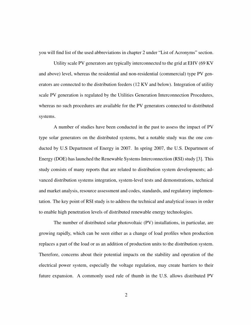
Utility scale PV generators are typically interconnected to the grid at EHV (69 KV
and above) level, whereas the residential and non-residential (commercial) type PV gen-
erators are connected to the distribution feeders (12 KV and below). Integration of utility
scale PV generation is regulated by the Utilities Generation Interconnection Procedures,
whereas no such procedures are available for the PV generators connected to distributed
systems.
A number of studies have been conducted in the past to assess the impact of PV
type solar generators on the distributed systems, but a notable study was the one con-
ducted by U.S Department of Energy in 2007. In spring 2007, the U.S. Department of
Energy (DOE) has launched the Renewable Systems Interconnection (RSI) study [3]. This
study consists of many reports that are related to distribution system developments; ad-
vanced distribution systems integration, system-level tests and demonstrations, technical
and market analysis, resource assessment and codes, standards, and regulatory implemen-
tation. The key point of RSI study is to address the technical and analytical issues in order
to enable high penetration levels of distributed renewable energy technologies.
The number of distributed solar photovoltaic (PV) installations, in particular, are
growing rapidly, which can be seen either as a change of load profiles when production
replaces a part of the load or as an addition of production units to the distribution system.
Therefore, concerns about their potential impacts on the stability and operation of the
electrical power system, especially the voltage regulation, may create barriers to their
future expansion. A commonly used rule of thumb in the U.S. allows distributed PV
2
systems with peak powers up to 15% of the peak load on a feeder (or section) to be
permitted without a detailed impact study [4]. However, as total distributed PV units
increase on many feeders, a more rigorous study of the impacts of various PV penetration
levels on feeder voltages is justified.
1.1 Problem Statement
The voltage regulation of radial distribution system is accomplished by using on-
load tap changer at HV/MV substation and reactive power compensation upon the esti-
mated voltage raise/drop based on load profiles and load-flow calculations. The penetra-
tion of PV units (residential and commercial) at the load side reduces the load demand
which leads to reduce losses and improved voltage profile. Obviously, this is true as long
as the power flows in its conventional direction (from the substation into the end-user).
If a great amount of distributed PV generators is connected into the distribution system,
the flow of power may be reversed, from the load (distributed PV) towards the substation.
Consequently, there is a possible voltage rise along distribution feeders as a result of re-
verse power flow, especially at low demand and high generation conditions, and hence the
effectiveness of voltage regulation may be lost.
1.2 Purpose of Thesis
The reverse power flow of both active and reactive power components injected by
PV systems may lead to losing the voltage regulation, which is the most likely impact
caused by the high PV penetrations, for the distribution power system.
3
The purpose of this thesis is to investigate the voltage regulation of the system
during various levels of PV penetration and different inverter topologies every 30 minutes
of steady state operations and to estimate the maximum level of penetration, which will
not affect the stability and operation of the power system. Also, to review the capability
of existing inverter topologies to support the future growth of PV generators.
1.3 Rationale of Study
Two main rules, which have major influences in any study, were considered in this
thesis as study bases and these are:
• The load is variable: The load demands of different consumers vary upon their
activities and therefore the load in each bus is never constant. The consequences of
these changes have a direct impact on the voltage regulation of the bus, i.e. voltage
drop usually happens during peak load while the voltage rises during the light load
period.
• PV Generation is uncertain: The most common impact on the generated power from
PV units is the weather and the solar irradiation which leads to temporarily reduce
the PV capability of power generation. For example, clouds covering the sun can
cut Photovoltaic (PV) array and reduce the energy absorption by the solar panel
depending on how much daylight they diffuse. Also, twilight sun has an impact on
the generated power and has to be considered.
4
CHAPTER 2
BACKGROUND AND REVIEW
2.1 Definition of Terms
2.1.1 AC Power Classification
Real power (P): Power dissipated by a load is referred to as active power. Active
power is symbolized by the letter P and is measured in the unit of Watts (W);
P = V Icosϕ ′′W ′′ (1)
Reactive power (Q): Power merely absorbed and returned in load due to its reac-
tive properties is referred to as reactive power. Reactive power is symbolized by the letter
Q and is measured in the unit of Volt Amps reactive (VAr);
Q = V Isinϕ ′′V Ar′′ (2)
Phase angle (ϕ): the angle of difference (in degrees) between voltage and current.
This angle is the monitor of load behavior (resistive, inductive, or capacitive). If the phase
difference is zero (ϕ = 0) then the load is purely resistive. If the current leads the voltage
(quadrant IV operating region) then the load is inductive behavior. If the current lags the
voltage (quadrant I operating region) then the load is capacitive behavior.
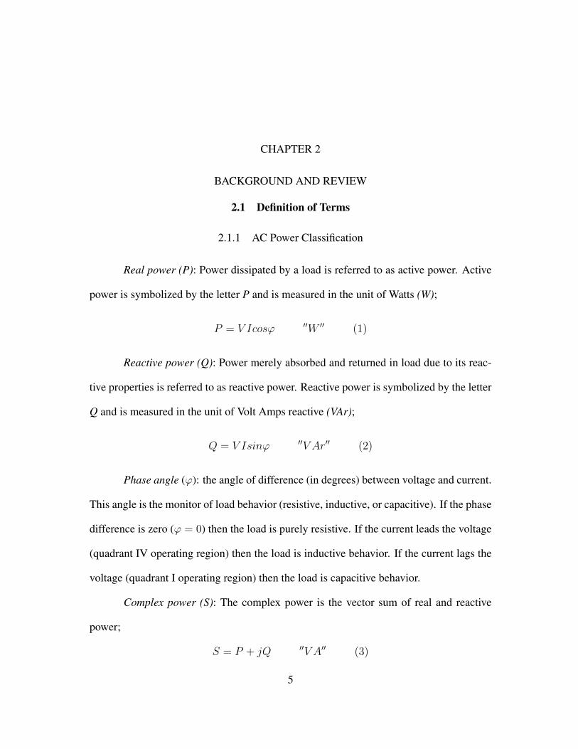
Complex power (S): The complex power is the vector sum of real and reactive
power;
S = P + jQ ′′V A′′ (3)
5
Apparent Power (|S|): The apparent power is the magnitude of the complex power;
|S| =√P 2 +Q2 ′′V A′′ (4)
Both apparent and complex power quantities are symbolized by the letter S and are
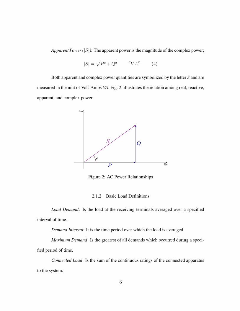
measured in the unit of Volt-Amps VA. Fig. 2, illustrates the relation among real, reactive,
apparent, and complex power.
Figure 2: AC Power Relationships
2.1.2 Basic Load Definitions
Load Demand: Is the load at the receiving terminals averaged over a specified
interval of time.
Demand Interval: It is the time period over which the load is averaged.
Maximum Demand: Is the greatest of all demands which occurred during a speci-
fied period of time.
Connected Load: Is the sum of the continuous ratings of the connected apparatus
to the system.
6
Demand Factor: It is the ratio of the maximum demand of a system to the total
connected load to that system.
Load Factor: It is the ratio of the average load to the peak load over a specified
period of time.
Load Diversity: It is the difference between the sum of two or more individual
peak loads and the peak of the combined load.
Diversity Factor: It is the ratio of the sum of individual maximum demands of
various subdivisions to the maximum demand of the entire system.
Utilization Factor: It is the ratio of the maximum demand of a system to the rated
capacity of the system.
Loss Factor: It is the ratio of the average power loss to the peak load power loss
during a specified period of time.
2.1.3 System Buses
Swing bus (or Slack bus): It is a reference bus for which V ∠ ϕ typically 1.0 ∠ 0◦
is input data while P and Q are unknown values.
Load (PQ) bus: P and Q are input data whereas V and ϕ are unknown. Most buses
in a typical system are load buses.
Voltage controlled (PV) bus: are buses to which generators, switched shunt ca-
pacitors, or static var systems are connected. P and V are input data while Q and ϕ are
unknown to be computed.
Primary bus: The connection point between the TL’s and the DS.
7
Secondary bus: Where the distributed power starts to flow towards the load.
Service entrance: The load side of the point of common coupling (PCC).
Utilization bus: The point of use where the outlet equipment is plugged in.
2.2 Voltage Instability Consequences
The following voltage stability definition is according to Definition and Classifi-
cation of Power System Stability by IEEE/CIGRE Joint Task Force on Stability Terms
and Definitions, 2004: According to Prabha Kundur [5], “Voltage stability refers to the
ability of a power system to maintain steady voltages at all buses in the system after being
subjected to a disturbance from a given initial operating condition”. Voltage instability
implies an uncontrolled drop/rise in voltage triggered by a disturbance, leading to voltage
regulation collapse and is primarily caused by dynamics connected with the load. There
are two categories of voltage instability; voltage drop and/or rise situations. The fluctua-
tion of the load is the main reason in the fluctuation of voltage profile in the utility grid.
Voltage drop is when voltage at sending end of a distribution line is higher than the voltage
at receiving end of the same line. Voltage drop usually occurs at maximum load case and
in starting operation of large motors. Excessive voltage drop, significantly, impairs the
starting and the operation of an electrical equipment (i.e. motors). Voltage drops could be
manipulated through appropriate location of power factor correction capacitors at some
buses of the distribution system. Voltage rise is opposite to voltage drop, the voltage at
sending end of a distribution line is lower than the voltage at receiving end of the same
line. The voltage rise is more severe when there is no demand (minimum load durations)
8
because all the local generation is exported back to the primary distribution substation.
For PV systems, when a grid-connected inverter produces ac current, the impedance from
the grid and inverter output circuit conductors causes an increase in voltage at the inverter
relative to the utility voltage. This phenomenon is commonly referred to as voltage rise.
2.3 PV Type Generator System
A solar cell is a very large p-n junction (or diode). PV cells convert sunlight into
electricity by an energy conversion process; photons of sunlight hit the cells, exciting
electrons in the atoms of a semi-conducting material. The freed electrons go into the
n-type layer while the holes go down into the p-type layer. The flow of these electrons
produce a DC current. An inverter is used for AC requirements. Silicon is the most
commonly used semi-conductor, due to its properties of acting like an insulator at room
temperature and a conductor after providing the supply. The following are definitions to
PV jargon:
• PV Module: A group of PV cells connected in series and/or parallel (as needed to
reach the specific voltage and current requirements) and encapsulated in an envi-
ronmentally protective laminate.
• PV Panel: A group of modules that is the basic building block of a PV array.
• PV Array: A group of panels that comprises the complete PV generating unit.
• PV Inverter: Converts DC power from the solar array into AC form.
9
Because of their modularity, PV systems can be designed to meet any electrical
requirement. Typically, PV systems are made of the following elements:
• PV modules, cables, and mounting or fixing hardware.
• An inverter and controller.
• Batteries, back-up generators, and other components in off-grid situations.
• Special electricity meters, in the case of grid-connected systems.
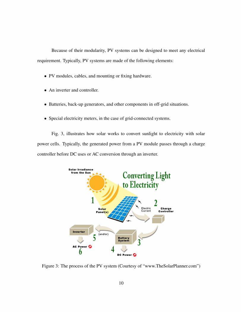
Fig. 3, illustrates how solar works to convert sunlight to electricity with solar
power cells. Typically, the generated power from a PV module passes through a charge
controller before DC uses or AC conversion through an inverter.
Figure 3: The process of the PV system (Courtesy of “www.TheSolarPlanner.com”)
10
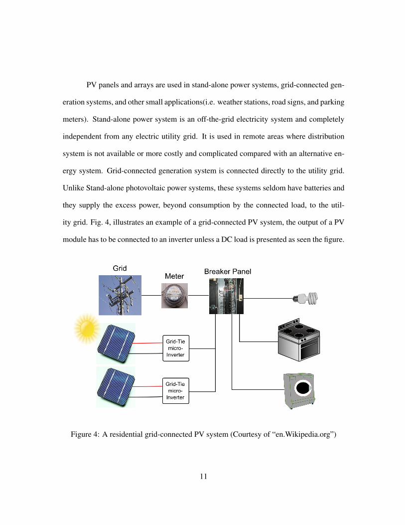
PV panels and arrays are used in stand-alone power systems, grid-connected gen-
eration systems, and other small applications(i.e. weather stations, road signs, and parking
meters). Stand-alone power system is an off-the-grid electricity system and completely
independent from any electric utility grid. It is used in remote areas where distribution
system is not available or more costly and complicated compared with an alternative en-
ergy system. Grid-connected generation system is connected directly to the utility grid.
Unlike Stand-alone photovoltaic power systems, these systems seldom have batteries and
they supply the excess power, beyond consumption by the connected load, to the util-
ity grid. Fig. 4, illustrates an example of a grid-connected PV system, the output of a PV
module has to be connected to an inverter unless a DC load is presented as seen the figure.
Figure 4: A residential grid-connected PV system (Courtesy of “en.Wikipedia.org”)
11
2.4 PV Inverter Principle
An inverter is a DC-to-AC converter which converts the variable direct current
(DC) output generated from a photovoltaic (PV) solar panel into a utility frequency al-
ternating current (AC) that can be used for AC applications or directly connected into an
electrical grid network. A solar or PV inverter is a critical component in a photovoltaic
system because it is designed to operate over a variable DC input voltage range in order
to perform a maximum power generation process under the continuously varying solar
irradiation and ambient temperature.
Standards such as IEEE 1547 and UL1741 state that the PV inverter shall not ac-
tively regulate the voltage at the PCC [3]. This means that PV inverters are designed
to operate at unity power factor (net active power produced) at anytime of generation
process. In reality, many inverters have the ability to regulate the voltage profile by pro-
viding/absorbing reactive power ,in addition to the generated active power by their PV
modules, to/from the electrical power system because their capabilities are measured by
their apparent power that combines both active and reactive power components, therefore;
providing/absorbing reactive power to/from the electrical grid depends on the inverter’s
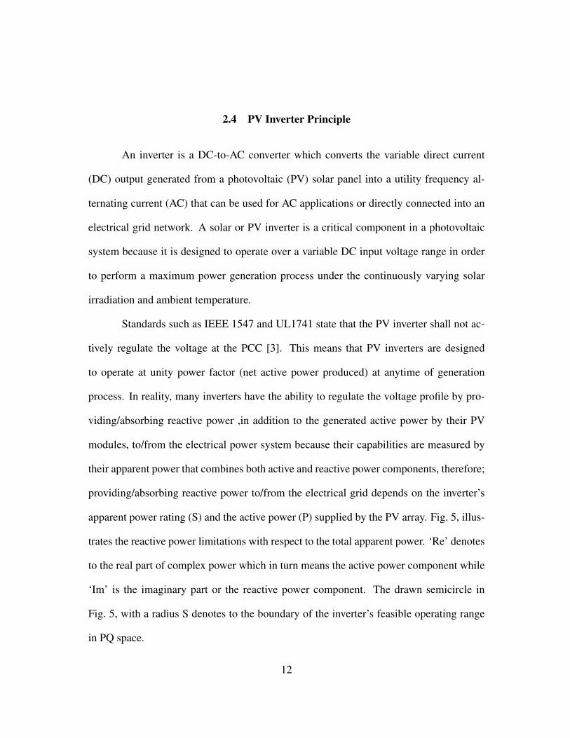
apparent power rating (S) and the active power (P) supplied by the PV array. Fig. 5, illus-
trates the reactive power limitations with respect to the total apparent power. ‘Re’ denotes
to the real part of complex power which in turn means the active power component while
‘Im’ is the imaginary part or the reactive power component. The drawn semicircle in
Fig. 5, with a radius S denotes to the boundary of the inverter’s feasible operating range
in PQ space.
12
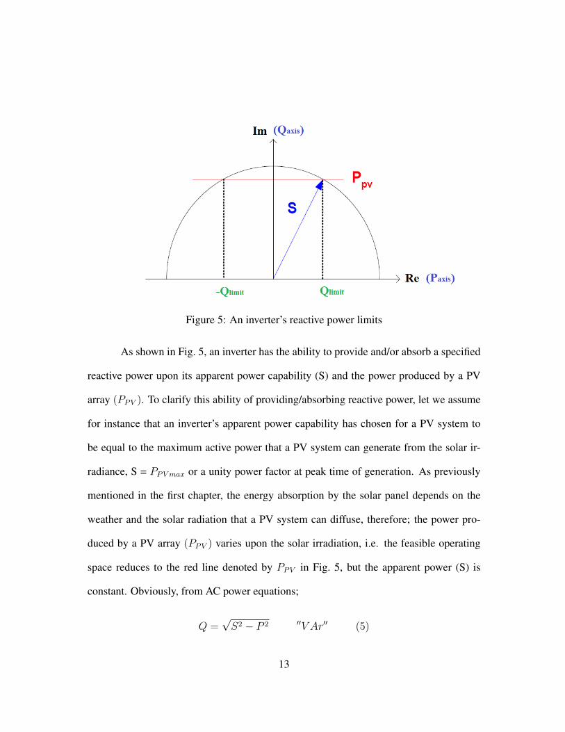
Figure 5: An inverter’s reactive power limits
As shown in Fig. 5, an inverter has the ability to provide and/or absorb a specified
reactive power upon its apparent power capability (S) and the power produced by a PV
array (PPV ). To clarify this ability of providing/absorbing reactive power, let we assume
for instance that an inverter’s apparent power capability has chosen for a PV system to
be equal to the maximum active power that a PV system can generate from the solar ir-
radiance, S = PPVmax or a unity power factor at peak time of generation. As previously
mentioned in the first chapter, the energy absorption by the solar panel depends on the
weather and the solar radiation that a PV system can diffuse, therefore; the power pro-
duced by a PV array (PPV ) varies upon the solar irradiation, i.e. the feasible operating
space reduces to the red line denoted by PPV in Fig. 5, but the apparent power (S) is
constant. Obviously, from AC power equations;
Q =√S2 − P 2 ′′V Ar′′ (5)
13
From Fig. 5, reactive power (Q) limits are found by the intersection points of the red line
segment with the semicircle, by projecting the end points of the segment down to the
Qaxis, these points are labeled as −Qlimit and Qlimit. This means that an inverter can
behave as an inductor or a capacitor upon the required voltage profile (provide or absorb a
reactive power). Also, an inverter can use its entire rating (S) to provide or absorb reactive
power (Q) if PPV equals zero (there is no sun), on the other hand, it has no Q capability
if PPV equals S (at Pmax generated by a PV array).
To provide reactive power injection while supplying maximum active power from
PV modules, it is necessary to increase the inverter size in order to increase the capability
of its rated power. By increasing the inverter size by 5%, making S = 1.05 PPVmax ,
the reactive power capability can be increased from zero to nearly 32% in the maximum
PV power generation condition. This will give the power factor range of unity to 0.95
leading/lagging. The Q capacity during no sun condition is then 105%. Fig. 6, illustrates
the active and reactive power capability of the inverter versus the its size.
Figure 6: Relationship between inverter size and its reactive power capability
14
2.5 List of Acronyms
AC Alternating Current
CIGRE (in French) Conseil International des Grands Reseaux Electriques
CIGRE (in English) International Council on Large Electric Systems
4 Delta
DC Direct Current
DG Distributed Generation
DS Distribution Substation
DOE Department of Energy
E Expected
EHV Extra High Voltage
GSO Glover, Sarma, and Overbye edition
GTM Greentech Media
GY Grounded Star (or Grounded Wye)
HV High Voltage
IEEE Institute of Electrical and Electronics Engineers
IJRER International Journal of Renewable Energy Research
Im Imaginary
KV Kilo Volt
MV Medium Voltage
MVA Mega Volt Ampere
MVAr Mega Volt Ampere reactive
15
MW Mega Watt
NREL National Renewable Energy Laboratory
PCC Point of Common Coupling
PF Power Factor
PU Per Unit
PV Photovoltaic
Re Real
RSI Renewable Systems Interconnection
SCB Shunt Capacitor Bank
SEIA Solar Energy Industries Association
TL Transmission Line
UL Underwriters Laboratories
WRT With Respect To
16

CHAPTER 3
METHODOLOGY
3.1 Approach
This thesis develops and tests a theoretical distibution power system and exam-
ines the factors that influence the adoption and acceptance of the selected network. The
following approach has been adopted in thesis:
• Selecting a representative distribution power system network from NREL study [6].
• Expanding the network to include a low-voltage service transformer and a sec-
ondary circuit.
• Loading the power system to nearly its capability with a mix of residential and
commercial load in the secondary circuit.
• Modeling the network with various typical voltage support equipment such as ca-
pacitors and voltage regulators.
• Simulating the model using a simulation program with various scenarios of PV
penetration levels and load profiles every 30 minutes.
• Investigating the voltage profile for each bus every 30 minutes with different PV
penetration and PV inverter topology scenarios.
17
In this thesis, PV penetration is defined as the ratio of total peak apparent power
of PV to peak load apparent power on the feeder:
PV Penetration = (PeakPV ApparentPower)/(PeakLoadApparentPower)
3.2 Data Gathering Method
Data gathering is an important aspect for any type of study. The choice of method
is influenced by the data collection strategy, the type of variable, and the accuracy re-
quired. Regardless of the field of study or preference for defining data, accurate data
collection is essential to maintaining the integrity of any study. Both the selection of ap-
propriate data collection instruments (existing, modified, or newly developed) and clearly
instructions for their correct use reduce the likelihood of errors occurring. Inaccurate data
collection can impact the results of a study and ultimately leads to invalid results. In this
thesis, we have used standards, previous researches, and the rule of thumb in gathering
the data.
The load profiles represent a mix of residential and commercial load and were
scaled with a load diversity factor of about 1.3 for each load class according to NREL
study [4]. The load diversity factor is defined as the ratio of the sum of the individual
maximum loads of various laterals of the system to the maximum demand of the entire
distribution system. The considered load behavior in thesis was normalized to reach its
maximum point at 100%. Fig. 7, shows final scaled and randomized total load profiles
(residential and commercial) for a typical feeder over two consecutive days (weekday and
weekend). As can be seen from Fig. 7, the load behavior is almost the same for both
18
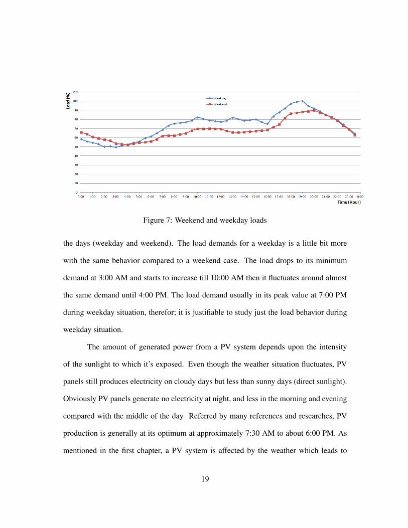
Figure 7: Weekend and weekday loads
the days (weekday and weekend). The load demands for a weekday is a little bit more
with the same behavior compared to a weekend case. The load drops to its minimum
demand at 3:00 AM and starts to increase till 10:00 AM then it fluctuates around almost
the same demand until 4:00 PM. The load demand usually in its peak value at 7:00 PM
during weekday situation, therefor; it is justifiable to study just the load behavior during
weekday situation.
The amount of generated power from a PV system depends upon the intensity
of the sunlight to which it’s exposed. Even though the weather situation fluctuates, PV
panels still produces electricity on cloudy days but less than sunny days (direct sunlight).
Obviously PV panels generate no electricity at night, and less in the morning and evening
compared with the middle of the day. Referred by many references and researches, PV
production is generally at its optimum at approximately 7:30 AM to about 6:00 PM. As
mentioned in the first chapter, a PV system is affected by the weather which leads to
19
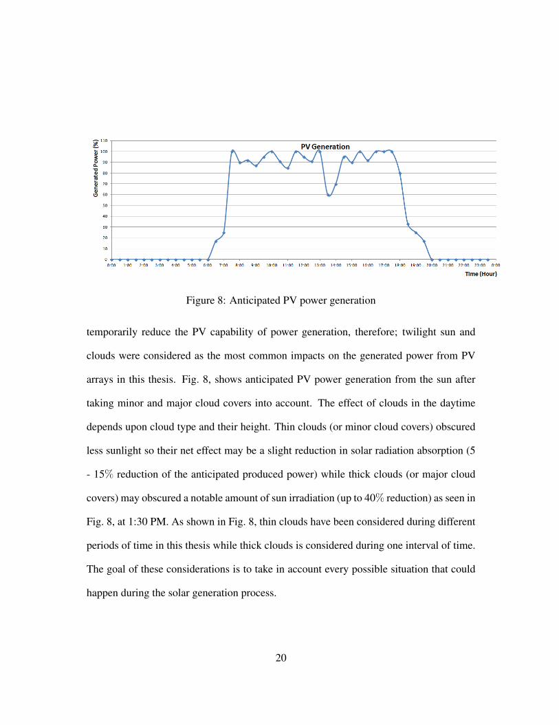
Figure 8: Anticipated PV power generation
temporarily reduce the PV capability of power generation, therefore; twilight sun and
clouds were considered as the most common impacts on the generated power from PV
arrays in this thesis. Fig. 8, shows anticipated PV power generation from the sun after
taking minor and major cloud covers into account. The effect of clouds in the daytime
depends upon cloud type and their height. Thin clouds (or minor cloud covers) obscured
less sunlight so their net effect may be a slight reduction in solar radiation absorption (5
- 15% reduction of the anticipated produced power) while thick clouds (or major cloud
covers) may obscured a notable amount of sun irradiation (up to 40% reduction) as seen in
Fig. 8, at 1:30 PM. As shown in Fig. 8, thin clouds have been considered during different
periods of time in this thesis while thick clouds is considered during one interval of time.
The goal of these considerations is to take in account every possible situation that could
happen during the solar generation process.
20

3.3 Selected Network of Study
A typical distribution system arrangement was selected from a previous NREL
study [6]. The selected network includes voltage control equipment such as on-load tap-
changing transformer and switched capacitors. The model was further modified and ex-
panded to represent service transformers and secondary circuits (end-user and most likely
the point of the PV inverter connection). The major assumptions were considered are:
• The considered distribution system operates in steady-state behavior and in its in-
tended manner for voltage regulation according to utility’s guidelines.
• The considered distribution system is radial and supplied by a medium-voltage
transformer equipped with a tap changer.
• The distribution system consists of 39 buses; slack, primary and secondary, 18 ser-
vice, and 18 utilization buses.
• The distribution system includes two main feeders with laterals and distributed
loads; feeder I supplies 11 service buses while feeder II seven buses.
• The load in each bus is a mix of residential and commercial loads.
• Distribution substation protections allow active and reactive power back feed.
• The PV units are clustered at the lateral buses of feeder I as one after the other with
equal magnitude upon the penetration level.
• Energy Storage devices are not considered.
21
• The model is suitable for examination of equipment interaction and the impact on
the feeder voltage profile at different PV penetration levels.
• The selected distribution system was modeled using PowerWorld Simulator 15
GSO; the system base is 100 MVA, bus 99999 is the infinite bus and it denotes
to the system swing or slack bus, bus 5 and 10 represent primary and secondary
distribution substation respectively, and all the load buses are modeled as PQ buses.
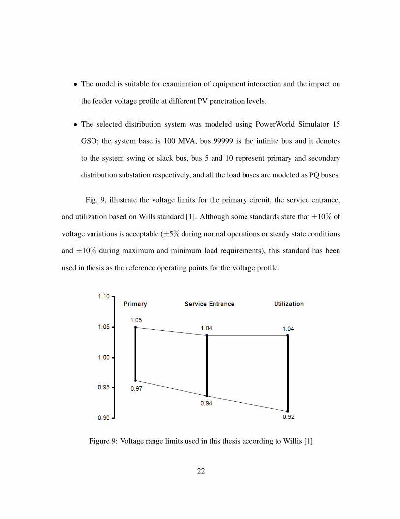
Fig. 9, illustrate the voltage limits for the primary circuit, the service entrance,
and utilization based on Wills standard [1]. Although some standards state that ±10% of
voltage variations is acceptable (±5% during normal operations or steady state conditions
and ±10% during maximum and minimum load requirements), this standard has been
used in thesis as the reference operating points for the voltage profile.
Figure 9: Voltage range limits used in this thesis according to Willis [1]
22

3.4 Major Component Data and Assumption
Because the resistive part (R) of a transformer impedance is very small compared
with the inductive part (X), it has been neglected. Also, the susceptance (B) which denotes
to the imaginary part of admittance of a transmission line is neglected. The models of the
major components in this thesis were assumed to be of typical values and described as
follow:
3.4.1 Transformers
The main transformer (substation transformer) was modeled as tap-changing trans-
former. The tap range is ± 10% of rated and the step voltage is 0.00625. The impedance
of the main transformer (69 4 / 12.47 GY ) KV is assumed as 5% on its rating with an
X/R ratio of 2.5. The impedance of each service transformers (12.47 GY / 0.48 GY) KV
is assumed as 2.5% [7] on its rating with an X/R ratio of 1.5. To insert the impedance
for each transformer in the program, the following formulas were used to determine each
impedance in PU upon the specified bases.
Z0(%) = ZPU(100MVAbase) × (MVATransformerbase ÷MVA100MVAbase)× 100 (6)
Z0 = ZPU(100MVAbase) ×MVATransformerbase % (7)
ZPU(100MVAbase) = Z0 ÷MVATransformerbase PU (8)
Table 1 shows the transformer ratings used in this distribution system.
23
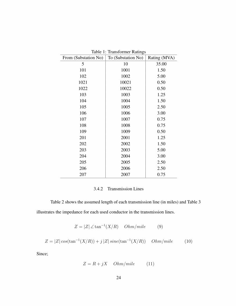
Table 1: Transformer RatingsFrom (Substation No) To (Substation No) Rating (MVA)
5 10 35.00101 1001 1.50102 1002 5.00
1021 10021 0.501022 10022 0.50103 1003 1.25104 1004 1.50105 1005 2.50106 1006 3.00107 1007 0.75108 1008 0.75109 1009 0.50201 2001 1.25202 2002 1.50203 2003 5.00204 2004 3.00205 2005 2.50206 2006 2.50207 2007 0.75
3.4.2 Transmission Lines
Table 2 shows the assumed length of each transmission line (in miles) and Table 3
illustrates the impedance for each used conductor in the transmission lines.
Z = |Z|∠ tan−1(X/R) Ohm/mile (9)
Z = |Z| cos(tan−1(X/R)) + j |Z| sine(tan−1(X/R)) Ohm/mile (10)
Since;
Z = R + jX Ohm/mile (11)
24
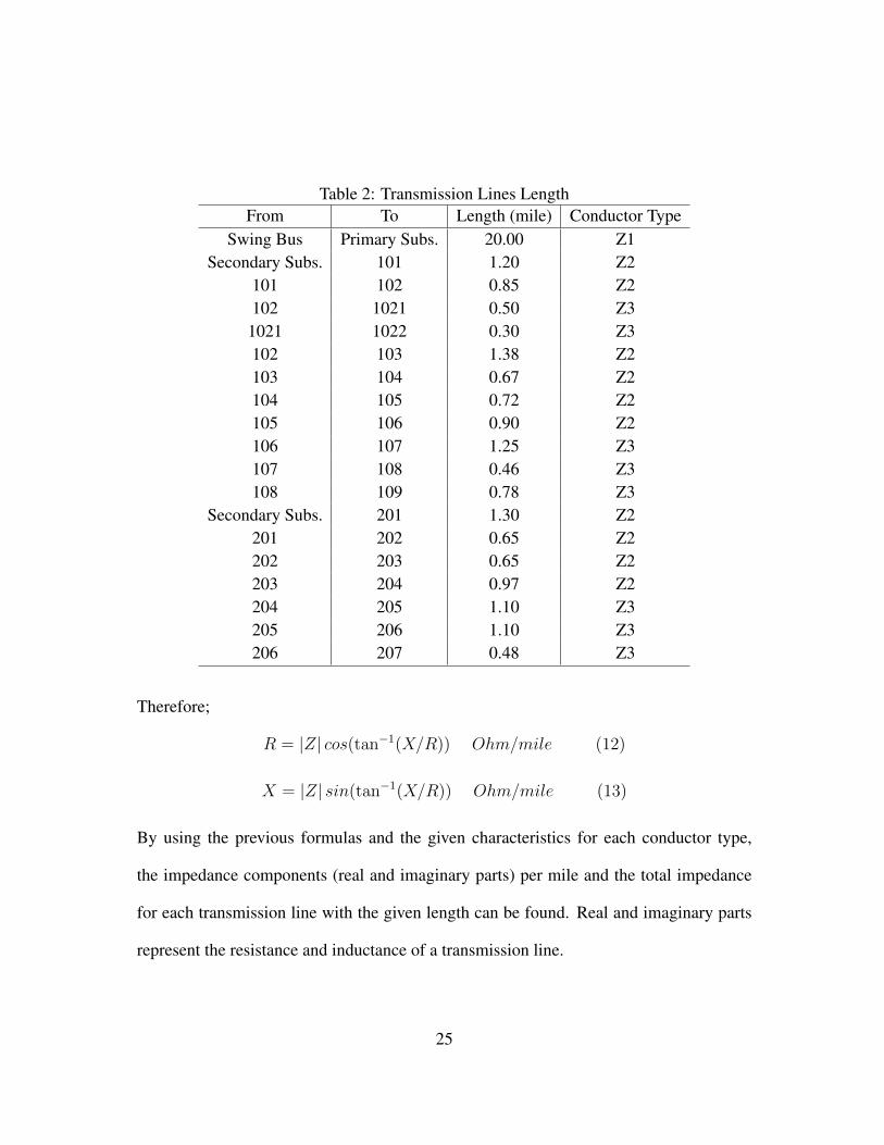
Table 2: Transmission Lines LengthFrom To Length (mile) Conductor Type
Swing Bus Primary Subs. 20.00 Z1Secondary Subs. 101 1.20 Z2
101 102 0.85 Z2102 1021 0.50 Z3
1021 1022 0.30 Z3102 103 1.38 Z2103 104 0.67 Z2104 105 0.72 Z2105 106 0.90 Z2106 107 1.25 Z3107 108 0.46 Z3108 109 0.78 Z3
Secondary Subs. 201 1.30 Z2201 202 0.65 Z2202 203 0.65 Z2203 204 0.97 Z2204 205 1.10 Z3205 206 1.10 Z3206 207 0.48 Z3
Therefore;
R = |Z| cos(tan−1(X/R)) Ohm/mile (12)
X = |Z| sin(tan−1(X/R)) Ohm/mile (13)
By using the previous formulas and the given characteristics for each conductor type,
the impedance components (real and imaginary parts) per mile and the total impedance
for each transmission line with the given length can be found. Real and imaginary parts
represent the resistance and inductance of a transmission line.
25

Table 3: Conductor Characteristic[Z] (ohm/mile) X/R Ratio
Z1 0.366 1.73Z2 0.648 2.00Z3 0.768 2.00
3.4.3 Load
The load refers to the power consumed by a connected electrical equipment. The
load profiles were rescaled to reach the peak (maximum value) at 100%. This was done
by dividing the load in each interval of time by the peak point that the load can reach.
All loads were modeled in PowerWorld program as a constant power (active and reactive)
load. All loads have a power factor of 0.92, which is representative of the mixture of
residential and commercial loads. Table 4 shows the maximum load for each bus.
3.4.4 Capacitor Banks
A capacitor bank is a grouping of several identical capacitors interconnected in
parallel or in series with one another. Shunt capacitor banks (fixed or discrete) are mainly
installed to provide capacitive reactive compensation/power factor correction. The use
of SCBs has significantly increased because they are relatively inexpensive and can be
easily installed anywhere on the network. Its installation has other beneficial effects on the
system such as: improvement of the voltage drop at the load side, better voltage regulation
(if they were adequately designed), reduction of losses and reduction or postponement of
investments in transmission. Table 5 shows the provided shunt capacitors (Fixed and
Discrete) and their location in the distribution system.
26
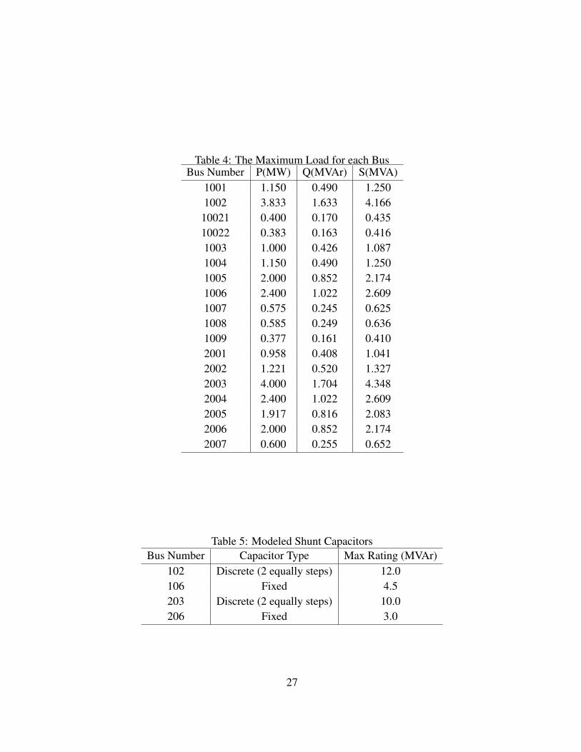
Table 4: The Maximum Load for each BusBus Number P(MW) Q(MVAr) S(MVA)
1001 1.150 0.490 1.2501002 3.833 1.633 4.166
10021 0.400 0.170 0.43510022 0.383 0.163 0.4161003 1.000 0.426 1.0871004 1.150 0.490 1.2501005 2.000 0.852 2.1741006 2.400 1.022 2.6091007 0.575 0.245 0.6251008 0.585 0.249 0.6361009 0.377 0.161 0.4102001 0.958 0.408 1.0412002 1.221 0.520 1.3272003 4.000 1.704 4.3482004 2.400 1.022 2.6092005 1.917 0.816 2.0832006 2.000 0.852 2.1742007 0.600 0.255 0.652
Table 5: Modeled Shunt CapacitorsBus Number Capacitor Type Max Rating (MVAr)
102 Discrete (2 equally steps) 12.0106 Fixed 4.5203 Discrete (2 equally steps) 10.0206 Fixed 3.0
27
3.4.5 Photovoltaic Systems
The word “photovoltaic” combines two terms; “photo” means light and “voltaic”
means voltage. Basically, a PV system is an arrangement of components designed to
supply usable electric power for a variety of purposes (DC and AC applications) using the
sun irradiation as the power source. Grid-connected photovoltaic power systems comprise
of Photovoltaic panels, solar inverters and their associated devices, protection units, and
grid connection equipment. The grid-connected PV system may supply excess power,
i.e. more than the connected load, to the utility grid. The PV system was modeled in
PowerWorld simulator as a generator model due to unavailability of the PV system in this
software. A generator can be used as a PV system in this software because of the available
options of control (active and reactive power flows).
3.5 Existing Network Behavior
PowerWorld is a power system visualization, simulation, and analysis tool de-
signed to simulate high voltage power system operation on a time frame ranging from
several minutes to several days. A one-line diagram for the selected network in Power-
Wold Simulator 15 GSO is shown in Fig. 10. The one-line diagram also shows the PV
unit locations in the system as assumed.
Fig. 11, through Fig. 13, illustrate the voltage behavior for each utilization, ser-
vice, and main substation (primary and secondary) bus in the system. Each figure demon-
strates the steady state voltage profile for a specified number of buses upon the system bus
type. Fig. 14, illustrates the supported reactive power via the provided shunt capacitors.
28
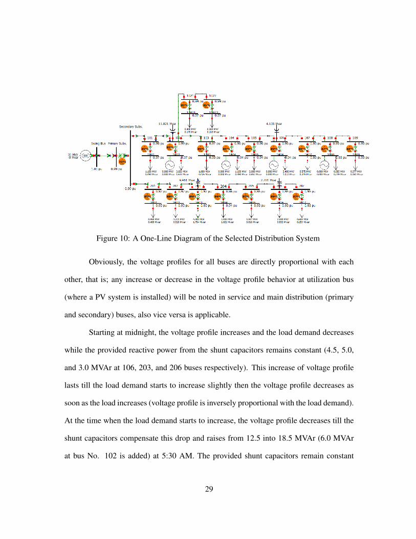
Figure 10: A One-Line Diagram of the Selected Distribution System
Obviously, the voltage profiles for all buses are directly proportional with each
other, that is; any increase or decrease in the voltage profile behavior at utilization bus
(where a PV system is installed) will be noted in service and main distribution (primary
and secondary) buses, also vice versa is applicable.
Starting at midnight, the voltage profile increases and the load demand decreases
while the provided reactive power from the shunt capacitors remains constant (4.5, 5.0,
and 3.0 MVAr at 106, 203, and 206 buses respectively). This increase of voltage profile
lasts till the load demand starts to increase slightly then the voltage profile decreases as
soon as the load increases (voltage profile is inversely proportional with the load demand).
At the time when the load demand starts to increase, the voltage profile decreases till the
shunt capacitors compensate this drop and raises from 12.5 into 18.5 MVAr (6.0 MVAr
at bus No. 102 is added) at 5:30 AM. The provided shunt capacitors remain constant
29
and the voltage profile fluctuates within the specified operating range till 8:00 AM then
the provided reactive power is increased to 23.5 MVAr (10.0 instead of 5.0 MVAr at
bus No 203). The voltage profile then fluctuates in a good operating range till 4:30 PM,
where a change in its profile is notable, the provided reactive power via shunt capacitors is
increased at 5:00 PM to 29.5 MVAr (extra 6.0 MVAr is supported at bus No 102). At 7:00
PM, the load reaches its maximum demand and as consequent the voltage profile drops
but still lies within the specified operating range. At 8:30 PM the supported reactive power
component starts to decrease into 23.5 MVAr at 9:00 PM. At this time, the voltage profile
decreases to its minimum point of operating range (at the edge with compared with the
used standard) whereas the provided reactive power through the shunt capacitors remain
the same. After this peak time of demand, the load starts to decrease gradually and the
voltage profile begins to improve, also, the provided reactive power is decreased slightly
(in the conventional steps) till it reduced to 18.5 MVAr (6.0, 4.5, 5.0, and 3.0 MVA at 102,
106, 203, and 206 buses) at 11:30 PM.
The voltage profile for the main substation lies from 0.985 to 1.005 PU. The volt-
age profiles for the service buses range from 0.94 to 1.04 PU. The voltage profiles for
the utilization buses vary from 0.935 to approximately 1.03 PU. From Wills standard [1],
the operating ranges of the voltage profile are; 0.97 to 1.05 PU for the main substation
(primary and secondary buses), 0.94 to 1.04 PU for the service buses, and 0.92 to 1.04 PU
for the utilization buses. By comparing these values with the used reference standard, we
found that the system works within the limited range.
30

Figure 11: The Steady-State Voltage Profile - Utilization Buses (No PV Penetration)
Figure 12: The Steady-State Voltage Profile - Service Buses (No PV Penetration)
31

Figure 13: The Steady-State Voltage Profile - Main Substation (No PV Penetration)
Figure 14: Provided shunt capacitors during Steady-State Conditions (No PV Penetration)
32
CHAPTER 4
PRESENTATION OF FINDINGS
In normal operating conditions, the feeder voltage profile decreases as the load
demand on that feeder increases whereas this situation is reflected once the load demand
starts to decrease and it may become higher than the voltage specified by the utility’s
guidelines. A baseline can be defined as a benchmark that is used as a foundation for
measuring or comparing current and past values. In this thesis, a Wills standard [1] has
been used as the voltage limits for the primary circuit, the service entrance, and utilization
bus. We have considered four baselines in our study upon different PV inverter typologies.
Each baseline has included different PV penetration levels. The PV units are connected
to feeder I and therefore the penetration of PV units is limited to the total connected load
of that feeder. The results were obtained in steady state conditions.
4.1 Baseline 1: SPV = PPV
In the first baseline configuration, an inverter that is compliant with IEEE 1547
and UL1741 “an inverter shall not actively regulate the voltage at the PCC” or an inverter
operates at a unity power factor at anytime of generation process, has been used. This
topology of operation for the inverter is considered as the worst case inverter’s topology
scenario because it does not provide a reactive power component. A reactive power com-
ponent is an important role in controlling the active power flow through the distribution
33
system (it acts like a traffic light in controlling the active power flow) and it has a tremen-
dous effect for the voltage profile of the distribution system(it raises the voltage drop in
the conventional direction of power flow and minimizes the voltage rise in reverse direc-
tion of power flow). The conventional flow of power is from the distribution substation
towards the load. In this baseline, three different PV penetration levels (10%, 20%, and
40%) have been discussed.
4.1.1 10% PV Penetration
The PV penetration is defined as the contribution amount of power in percentage
from a PV module with respect to a specified distribution feeder’s load.
PVPenetration = (PeakPVApparentPower)/(PeakLoadApparentPower)
A major factor in determining the impacts of PV generation is an understanding of the
amount of system peak load demand that can be expected to be reduced, resulting from
an ongoing uptake of PV’s. In this thesis, the penetration level was taken with respect to
the load on feeder I. For example, the penetration level of PV module at maximum load
on feeder I is 1.5058 MVA (10% x 15.058 MVA).
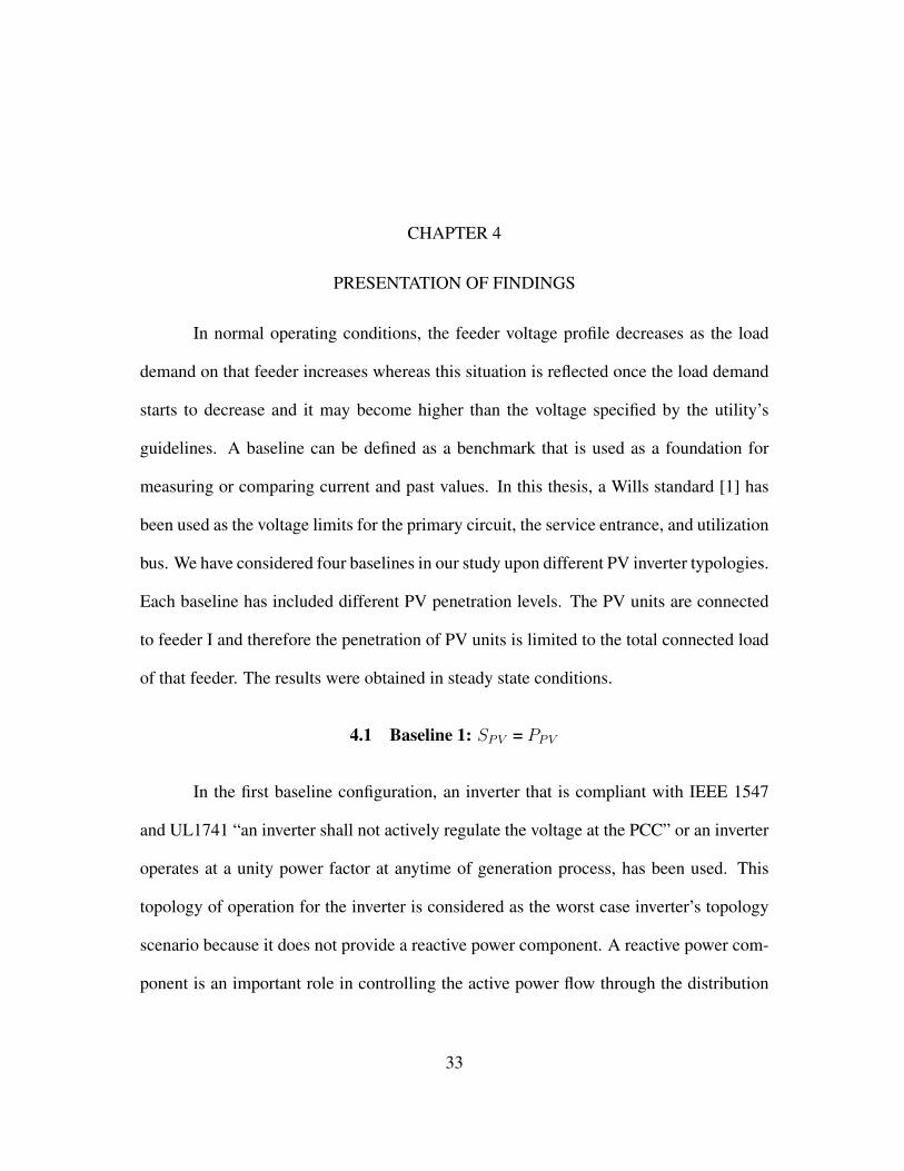
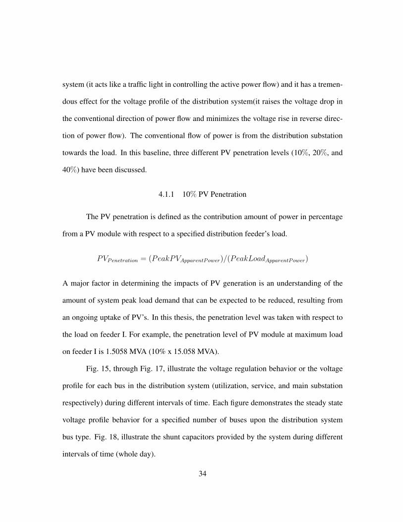
Fig. 15, through Fig. 17, illustrate the voltage regulation behavior or the voltage
profile for each bus in the distribution system (utilization, service, and main substation
respectively) during different intervals of time. Each figure demonstrates the steady state
voltage profile behavior for a specified number of buses upon the distribution system
bus type. Fig. 18, illustrate the shunt capacitors provided by the system during different
intervals of time (whole day).
34
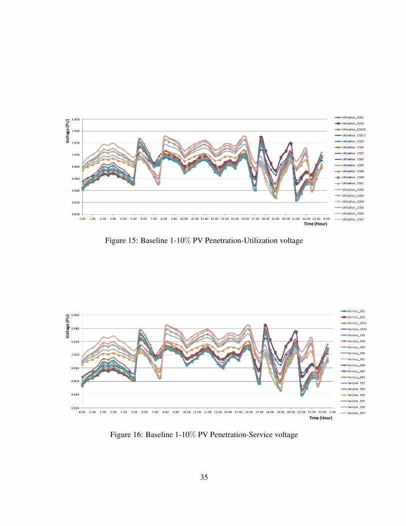
Figure 15: Baseline 1-10% PV Penetration-Utilization voltage
Figure 16: Baseline 1-10% PV Penetration-Service voltage
35
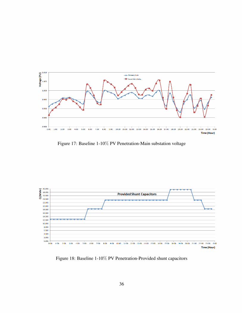
Figure 17: Baseline 1-10% PV Penetration-Main substation voltage
Figure 18: Baseline 1-10% PV Penetration-Provided shunt capacitors
36
As shown from Fig. 15, through Fig. 17, the voltage behavior for utilization buses
(where PV systems are installed) are directly proportional with service and main substa-
tion buses; any increase or decrease in the voltage profile at utilization bus will result in
an increase or decrease in the corresponding service bus and will have the same impact in
the main substation buses (primary and secondary).
Beginning with midnight, the voltage profile increases and the load demand de-
creases while the supported reactive power component from the provided shunt capacitors
starts at 12.5 MVAr (4.5, 5.0, and 3.0 MVAr at 106, 203, and 206 buses respectively).
This increase of voltage profile lasts till the load demand starts to increase slightly then
the voltage profile decreases as soon as the load increases (voltage profile is inversely
proportional with the load demand). At the time when the load demand starts to increase,
the voltage profile decreases till the shunt capacitors compensate this decrease and raises
from 12.5 into 18.5 MVAr (additional reactive power injection by the switched capaci-
tor at bus No. 102 is evident from the Q jump from 12.5 into 18.5 MVAr) at 5:30 AM.
The provided shunt capacitors remain constant and the voltage profile gradually drops
but within the specified operating range till 8:00 AM then the provided reactive power
is increased to 23.5 MVAr (10.0 instead of 5.0 MVAr at bus No 203) to compensate the
resultant voltage drop. The voltage profile then fluctuates in a good operating range till
5:00 PM, where a drop in its profile is notable, the provided reactive power via shunt ca-
pacitors is increased at 5:30 PM to 29.5 MVAr (additional 6.0 MVAr is supported at bus
No 102). At 7:00 PM, the load reaches its maximum demand and the voltage profile drops
as consequent of this increase but still lies within the specified range of operation. After
37
this peak time of demand, the load starts to decrease gradually and the voltage profile
begins to improve until 8:30 PM, where the provided reactive power component by the
system starts to decrease into 23.5 MVAr at 9:00 PM. At this time, a change in voltage
profile is notable (drops to its minimum operating point compared to the specified range
of operation, almost right on the edge with compared with the used standard). Finally, the
provided reactive power is decreased slightly (in the conventional steps) till it reduced to
18.5 MVAr (6.0, 4.5, 5.0, and 3.0 MVA at 102, 106, 203, and 206 buses) at 11:30 PM.
The voltage profile for the main substation lies from 0.985 to almost 1.005 PU.
The voltage profiles for the service buses range from approximately 0.94 to 1.045 PU.
The voltage profiles for the utilization buses ranges from 0.925 to around 1.03 PU. By
comparing these values with the used reference standard, the maximum operating point
for the service bus voltages is a little more than the one which is specified in the used
standard (+0.005 PU) but its to small and it can be neglected, so, the system works within
acceptable range.
4.1.2 20% PV Penetration
Herein, the PV penetration is doubled compared with the previous case (2 x 10%).
At peak load in feeder I, 15.058 MVA, the PV penetration level reaches around 3.012
MVA. Fig. 19, through Fig. 21, illustrate the voltage regulation behavior for each bus in
the distribution system (utilization, service, and main substation buses) during different
intervals of time. Fig. 18, illustrate the shunt capacitors provided by the system during
the time.
38

Figure 19: Baseline 1-20% PV Penetration-Utilization voltage
Figure 20: Baseline 1-20% PV Penetration-Service voltage
39
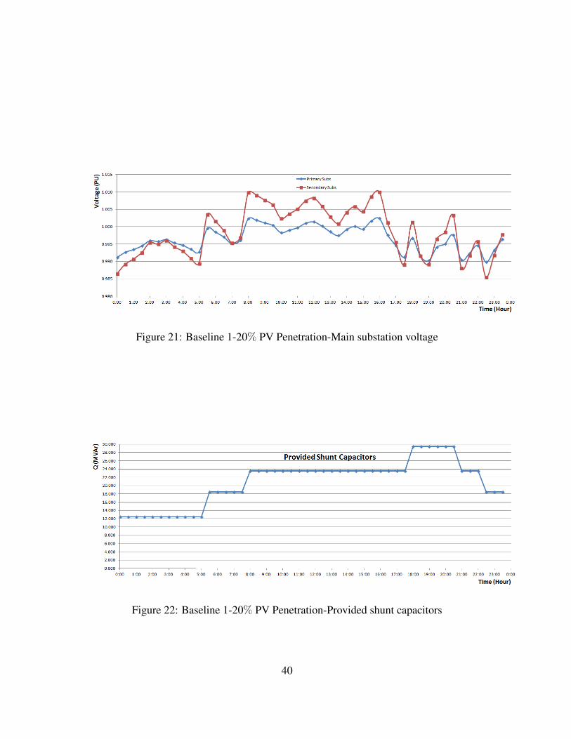
Figure 21: Baseline 1-20% PV Penetration-Main substation voltage
Figure 22: Baseline 1-20% PV Penetration-Provided shunt capacitors
40

At midnight, where the load is about 60% of peak demand, the supported reactive
power component from the provided shunt capacitors is 12.5 MVAr (4.5, 5.0, and 3.0
MVAr at 106, 203, and 206 buses respectively) and the voltage profile for each bus in
the distribution is within the specified operating range. The load demand decreases and
the voltage profile increases gradually till around 1.02 PU (as a maximum reached point)
for utilization and service buses at 2:00 AM. This behavior lasts about an hour then the
voltage profile decreases while the load demand starts to increase notably. At 5:30 AM,
additional reactive power is injected through bus No. 102 (6.0 MVAr) to compensate the
resultant voltage drop due to the load demand rise (the load at this time reaches 60%
of maximum demand). The provided shunt capacitors remain constant and the voltage
profile gradually drops but within the specified operating range till 8:00 AM where a
sudden jump in voltage profile is notable due to the additional injection of reactive power
at bus No 203 (10.0 instead of 5.0 MVAr). This increase of the provided reactive power,
a total of 23.5 MVAr, is a logically to compensate the resultant voltage drop. The voltage
profile then fluctuates in a good operating range till 5:30 PM, where a drop in its profile
is remarkable , the provided reactive power via shunt capacitors is increased at 6;00 PM
to 29.5 MVAr (additional 6.0 MVAr is supported at bus No 102). At 7:00 PM, the load
reaches its maximum demand and the voltage profile drops as consequent of this increase
but still lies within the specified range of operation. After this peak time of demand, the
load starts to decrease gradually and the voltage profile begins to improve until 8:30 PM,
where the provided reactive power component by the system starts to decrease into 23.5
MVAr at 9:00 PM. At this time, a change in voltage profile is noteworthy (drops to its
41
minimum operating point compared to the specified range of operation, almost right on
the edge for the utilization bus with compared to the used standard). Finally, the provided
reactive power is decreased slightly (in the conventional steps) till it reduced to 18.5 MVAr
(6.0, 4.5, 5.0, and 3.0 MVA at 102, 106, 203, and 206 buses) at 11:30 PM.
The voltage profile for the main substation lies from 0.985 to almost 1.01 PU.
The voltage profiles for the service buses range from approximately 0.94 to 1.05 PU.
The voltage profiles for the utilization buses ranges from 0.925 to around 1.04 PU. By
comparing these values with the used reference standard, the maximum operating point
for the service bus voltages is more than the one which is specified in the used standard
(+0.01 PU). As a result, it can be accepted as a normal operation in case of considering a
permitted error of ± 1%.
4.1.3 40% PV Penetration
In this case, the PV penetration at peak load is 6.023 MVA. This level of pen-
etration is divided over four buses in equally magnitude (1002, 1004, 1006, and 1008
utilization buses). Fig. 23, through Fig. 25, illustrate the voltage regulation or the volt-
age profile behavior for each bus in the distribution system (utilization, service, and main
substation respectively) during different intervals of time (every 30 minutes). Each figure
demonstrates the steady state voltage profile behavior for the specified buses upon the
distribution system bus type. Fig. 26, illustrates the provided shunt capacitors by 102,
106, 203, and 206 service buses in the distribution system during the specified intervals
of time (every 30 minutes).
42
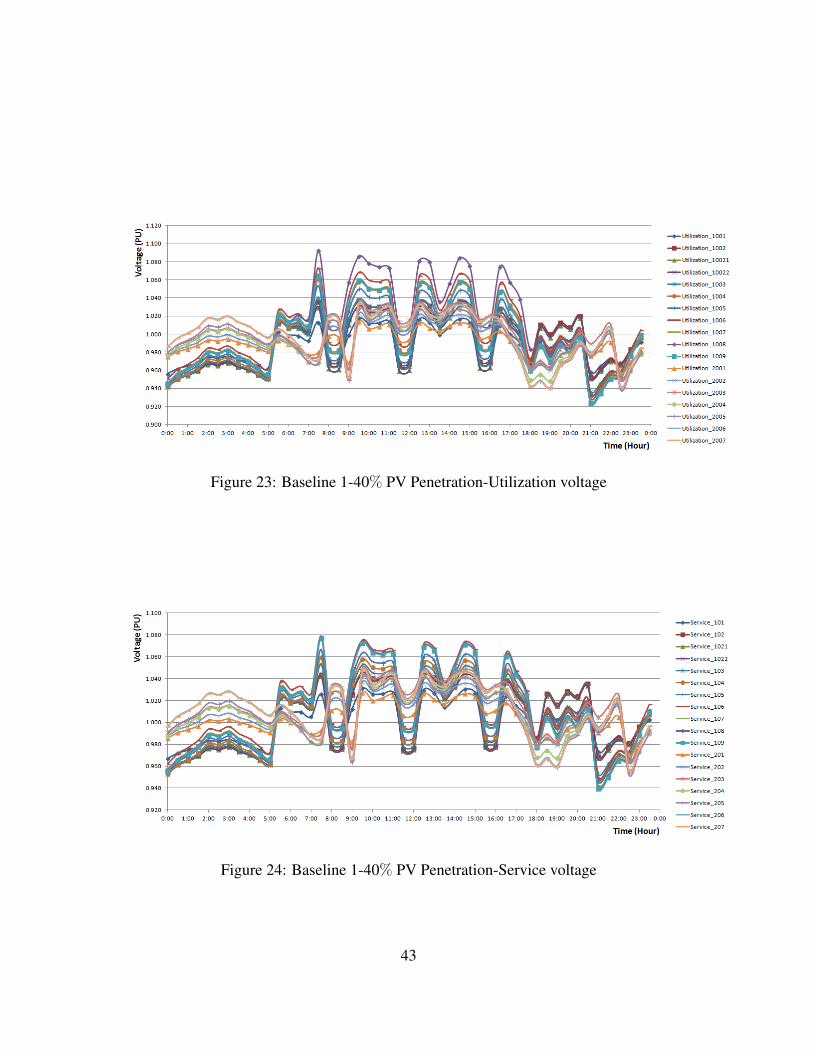
Figure 23: Baseline 1-40% PV Penetration-Utilization voltage
Figure 24: Baseline 1-40% PV Penetration-Service voltage
43

Figure 25: Baseline 1-40% PV Penetration-Main substation voltage
Figure 26: Baseline 1-40% PV Penetration-Provided shunt capacitors
44
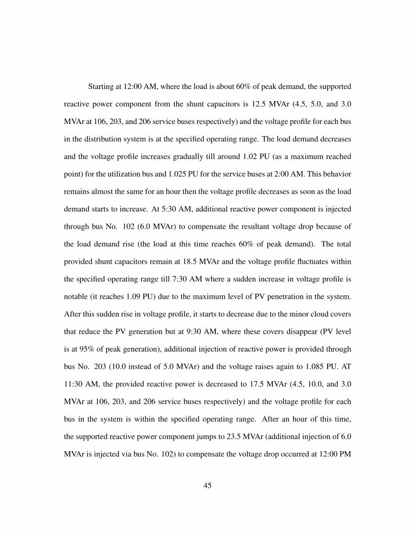
Starting at 12:00 AM, where the load is about 60% of peak demand, the supported
reactive power component from the shunt capacitors is 12.5 MVAr (4.5, 5.0, and 3.0
MVAr at 106, 203, and 206 service buses respectively) and the voltage profile for each bus
in the distribution system is at the specified operating range. The load demand decreases
and the voltage profile increases gradually till around 1.02 PU (as a maximum reached
point) for the utilization bus and 1.025 PU for the service buses at 2:00 AM. This behavior
remains almost the same for an hour then the voltage profile decreases as soon as the load
demand starts to increase. At 5:30 AM, additional reactive power component is injected
through bus No. 102 (6.0 MVAr) to compensate the resultant voltage drop because of
the load demand rise (the load at this time reaches 60% of peak demand). The total
provided shunt capacitors remain at 18.5 MVAr and the voltage profile fluctuates within
the specified operating range till 7:30 AM where a sudden increase in voltage profile is
notable (it reaches 1.09 PU) due to the maximum level of PV penetration in the system.
After this sudden rise in voltage profile, it starts to decrease due to the minor cloud covers
that reduce the PV generation but at 9:30 AM, where these covers disappear (PV level
is at 95% of peak generation), additional injection of reactive power is provided through
bus No. 203 (10.0 instead of 5.0 MVAr) and the voltage raises again to 1.085 PU. AT
11:30 AM, the provided reactive power is decreased to 17.5 MVAr (4.5, 10.0, and 3.0
MVAr at 106, 203, and 206 service buses respectively) and the voltage profile for each
bus in the system is within the specified operating range. After an hour of this time,
the supported reactive power component jumps to 23.5 MVAr (additional injection of 6.0
MVAr is injected via bus No. 102) to compensate the voltage drop occurred at 12:00 PM
45
but the voltage raises above the specified operating limit (it reaches 1.08 PU at 12:30 PM).
The load demand is almost the same from 12:30 PM to 3:30 PM and the voltage profile
fluctuates in the range of 0.96 to 1.085 PU. At 3:30 PM, the supported reactive power
through the shunt capacitors drops to 17.5 MVAr and the load demand increases while
the voltage profile’s range diminishes (up to 1.075 PU). At 4:30 PM, the PV penetration
is at its optimum (100%) and the load demand increases gradually while the reactive
power component provided by the distribution system is 23.5 MVAr. After these sudden
changes in network behavior, the voltage profile oscillates in a good operating range till
9:00 PM, where there is no PV penetration. At this time, a drop in voltage profile for
the utilization buses (where PV systems are installed) is observable (∼= 0.92 PU, almost
right on the edge) in synchronizing with the reactive power component decrease which
becomes 17.5 MVAr. The voltage behavior for utilization buses is directly proportional
to the voltage profile of service and main substation buses. Finally, the voltage profile is
improved and the provided reactive power is decreased slightly (in the conventional steps)
whereas the load demand starts to decrease. The provided shunt capacitors by the system
reduced to 18.5 MVAr (6.0, 4.5, 5.0, and 3.0 MVA at 102, 106, 203, and 206 buses) at
11:30 PM.
The voltage profile for the main substation lies from 0.985 to almost 1.015 PU.
The voltage profiles for the service buses range from approximately 0.94 to about 1.08
PU. The voltage profiles for the utilization buses ranges from 0.925 to a little more than
1.09 PU. By comparing these values with the used reference standard, the operating points
for the utilization and service buses exceed the specified range of operation.
46
4.2 Baseline 2: Unity PF at PPVmax
As mentioned in chapter 2, many inverters have the ability to regulate the voltage
profile by providing/absorbing reactive power (in addition to the generated active power
by their PV modules) to/from the electrical power system because their capabilities are
measured by their apparent power that combines both active and reactive power com-
ponents, the capability of the used inverter in this baseline is sized to be equal to the
maximum active power generated from the PV module. This means that the inverter can
supply a reactive power component to the grid in proportional to 1.0 PF at maximum PPV ,
PF = 1.0 at PPVmax. By using equation (5), the Q capacity of the PV inverter varies with
time upon the absorbed energy by the PV module and can reach upto 100% in no sun
conditions.
4.2.1 40% PV Penetration
Obviously, as concluded from the first baseline (the worst case for the inverter
topology), a 40% of penetration level is the worst case scenario of PV systems, therefore;
this penetration level has been discussed in the following baselines. The corresponding
PV penetration level with respect to the peak load is 6.023 MVA (40% x 15.058 MVA)
divided over the specified utilization buses (1002, 1004, 1006, and 1008 buses). Fig. 27,
through Fig. 29, illustrate the voltage regulation behavior for each bus in the distribution
system (utilization, service, and main substation buses) during different intervals of time
(every 30 minutes). Fig. 30, illustrate the shunt capacitors provided by the distribution
system (at 102, 106, 203, and 206 service buses) during the specified intervals of time.
47
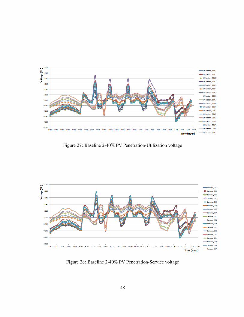
Figure 27: Baseline 2-40% PV Penetration-Utilization voltage
Figure 28: Baseline 2-40% PV Penetration-Service voltage
48
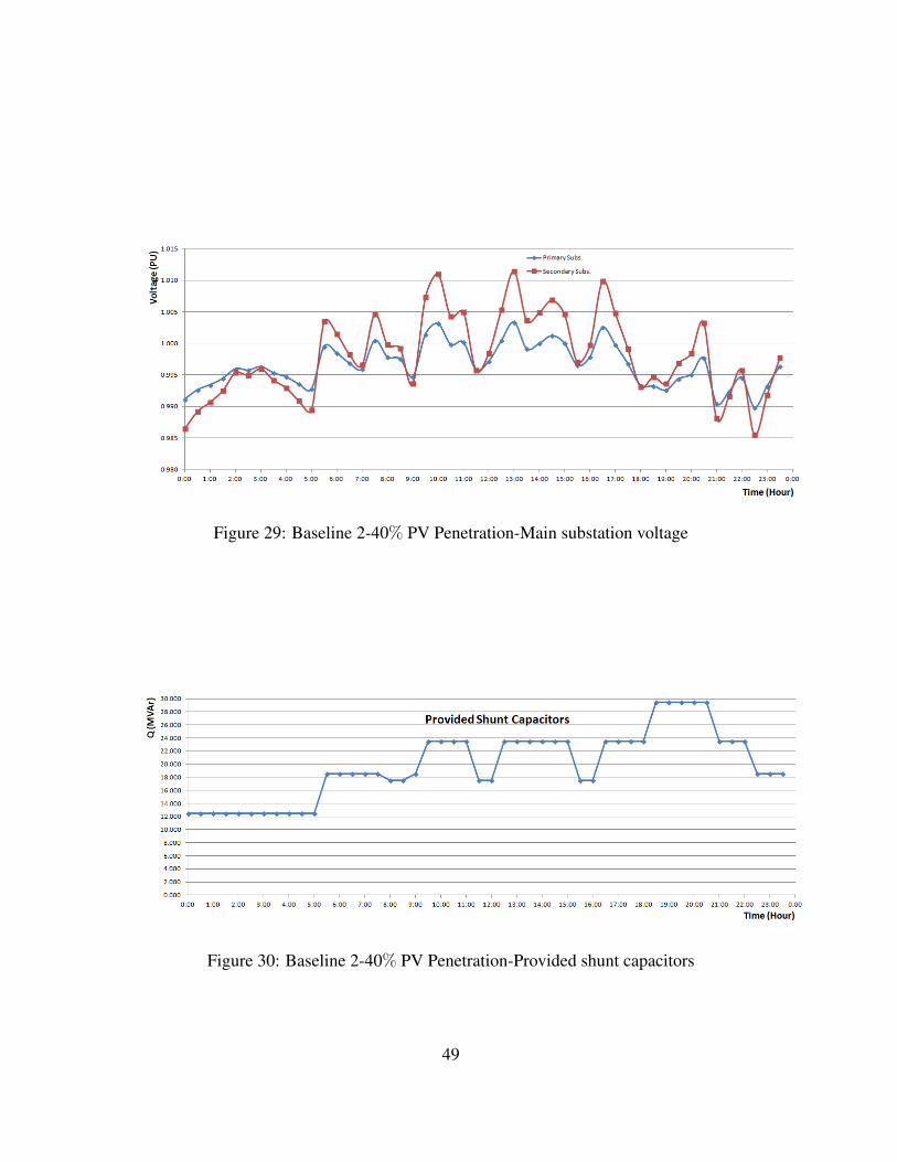
Figure 29: Baseline 2-40% PV Penetration-Main substation voltage
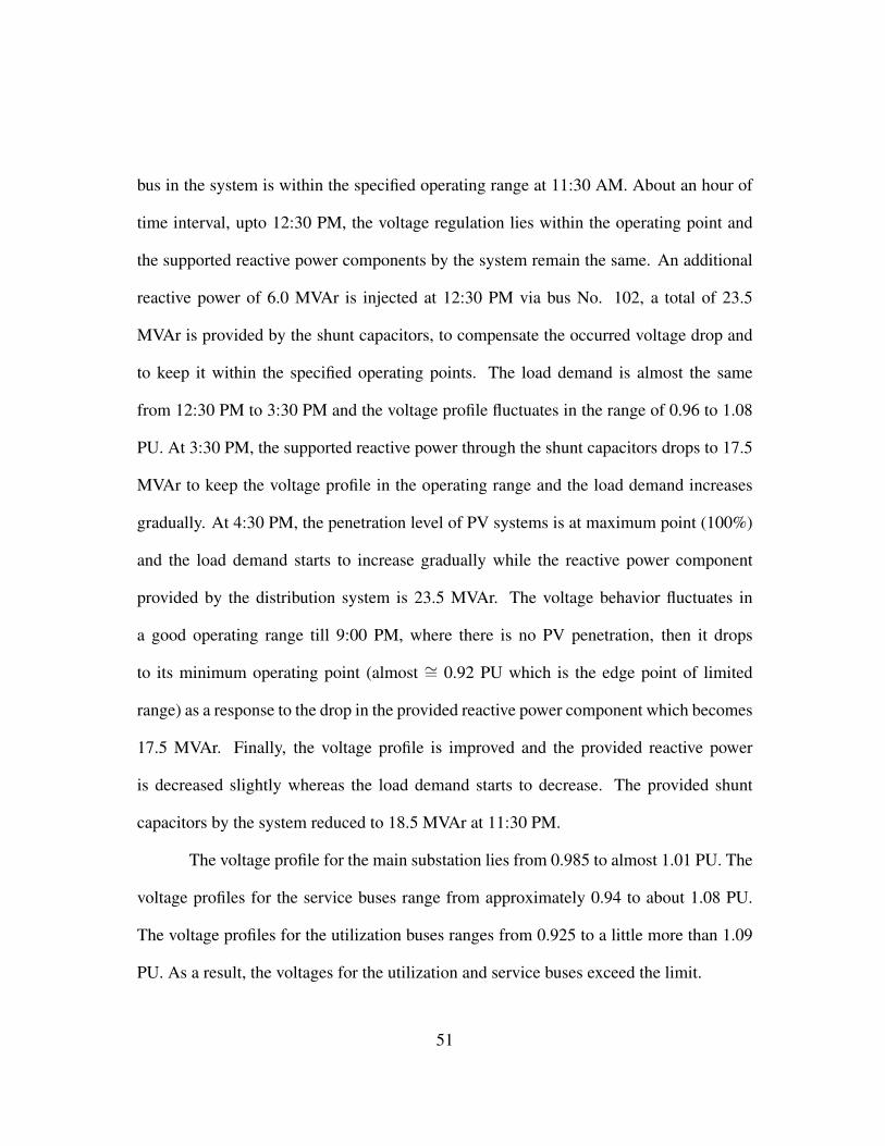
Figure 30: Baseline 2-40% PV Penetration-Provided shunt capacitors
49
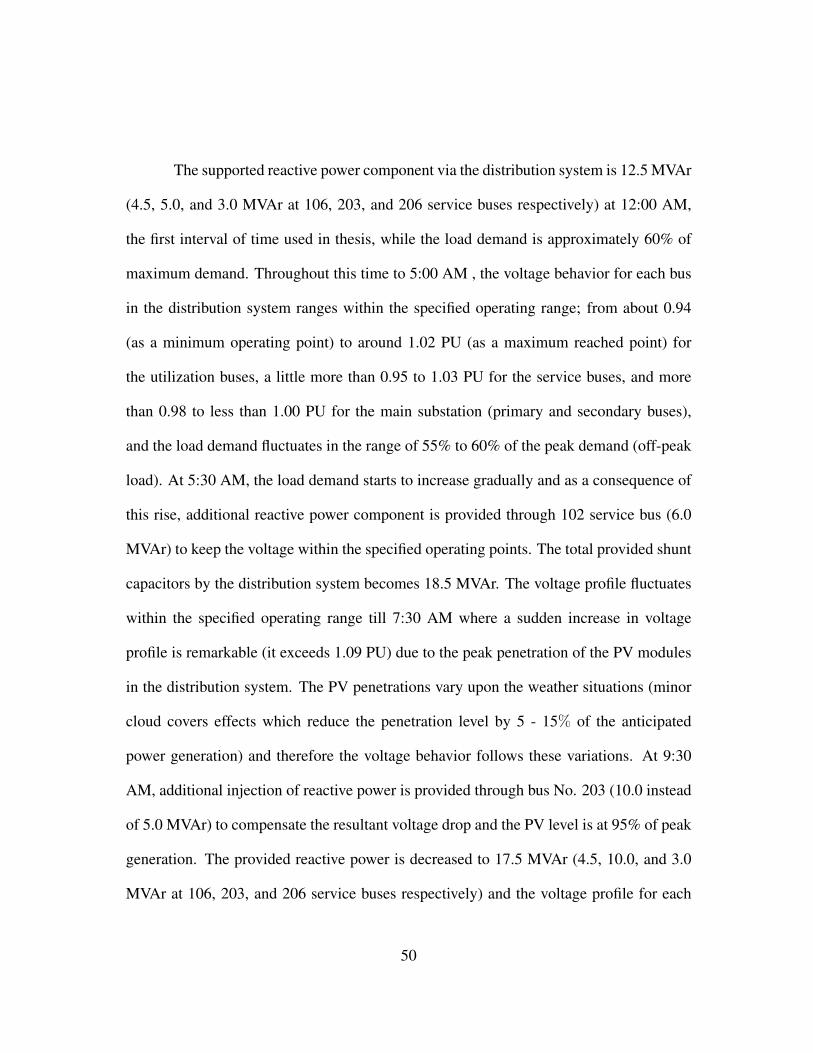
The supported reactive power component via the distribution system is 12.5 MVAr
(4.5, 5.0, and 3.0 MVAr at 106, 203, and 206 service buses respectively) at 12:00 AM,
the first interval of time used in thesis, while the load demand is approximately 60% of
maximum demand. Throughout this time to 5:00 AM , the voltage behavior for each bus
in the distribution system ranges within the specified operating range; from about 0.94
(as a minimum operating point) to around 1.02 PU (as a maximum reached point) for
the utilization buses, a little more than 0.95 to 1.03 PU for the service buses, and more
than 0.98 to less than 1.00 PU for the main substation (primary and secondary buses),
and the load demand fluctuates in the range of 55% to 60% of the peak demand (off-peak
load). At 5:30 AM, the load demand starts to increase gradually and as a consequence of
this rise, additional reactive power component is provided through 102 service bus (6.0
MVAr) to keep the voltage within the specified operating points. The total provided shunt
capacitors by the distribution system becomes 18.5 MVAr. The voltage profile fluctuates
within the specified operating range till 7:30 AM where a sudden increase in voltage
profile is remarkable (it exceeds 1.09 PU) due to the peak penetration of the PV modules
in the distribution system. The PV penetrations vary upon the weather situations (minor
cloud covers effects which reduce the penetration level by 5 - 15% of the anticipated
power generation) and therefore the voltage behavior follows these variations. At 9:30
AM, additional injection of reactive power is provided through bus No. 203 (10.0 instead
of 5.0 MVAr) to compensate the resultant voltage drop and the PV level is at 95% of peak
generation. The provided reactive power is decreased to 17.5 MVAr (4.5, 10.0, and 3.0
MVAr at 106, 203, and 206 service buses respectively) and the voltage profile for each
50
bus in the system is within the specified operating range at 11:30 AM. About an hour of
time interval, upto 12:30 PM, the voltage regulation lies within the operating point and
the supported reactive power components by the system remain the same. An additional
reactive power of 6.0 MVAr is injected at 12:30 PM via bus No. 102, a total of 23.5
MVAr is provided by the shunt capacitors, to compensate the occurred voltage drop and
to keep it within the specified operating points. The load demand is almost the same
from 12:30 PM to 3:30 PM and the voltage profile fluctuates in the range of 0.96 to 1.08
PU. At 3:30 PM, the supported reactive power through the shunt capacitors drops to 17.5
MVAr to keep the voltage profile in the operating range and the load demand increases
gradually. At 4:30 PM, the penetration level of PV systems is at maximum point (100%)
and the load demand starts to increase gradually while the reactive power component
provided by the distribution system is 23.5 MVAr. The voltage behavior fluctuates in
a good operating range till 9:00 PM, where there is no PV penetration, then it drops
to its minimum operating point (almost ∼= 0.92 PU which is the edge point of limited
range) as a response to the drop in the provided reactive power component which becomes
17.5 MVAr. Finally, the voltage profile is improved and the provided reactive power
is decreased slightly whereas the load demand starts to decrease. The provided shunt
capacitors by the system reduced to 18.5 MVAr at 11:30 PM.
The voltage profile for the main substation lies from 0.985 to almost 1.01 PU. The
voltage profiles for the service buses range from approximately 0.94 to about 1.08 PU.
The voltage profiles for the utilization buses ranges from 0.925 to a little more than 1.09
PU. As a result, the voltages for the utilization and service buses exceed the limit.
51
4.3 Baseline 3: 0.95 PF WRT PPV
In this baseline, the capability of the used inverter is sized to be 105% of the max-
imum active power produced from the PV module, that is; the reactive power capability
is increased from zero to nearly 32% at the maximum PV power generation condition
compared with the previous baseline (baseline 2). This means that the inverter topology
for providing a reactive power component to the grid is directly proportional to the ac-
tive power generated from the PV module with a 0.95 leading/lagging power factor (the
inverter can behave as both an inductor ”absorb a reactive power component” and a ca-
pacitor ”provide a reactive power component” upon the required voltage profile). The Q
capacity during no sun condition for the inverter is then 0% (because Q is proportional to
the generated P from the PV system).
4.3.1 40% PV Penetration
As mentioned before, a 40% of penetration level is corresponding to 6.023 MVA
with respect to the peak load demand and divided over the specified utilization buses
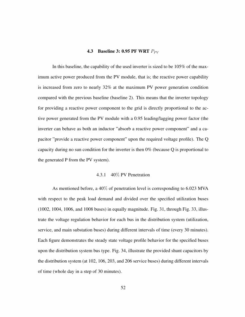
(1002, 1004, 1006, and 1008 buses) in equally magnitude. Fig. 31, through Fig. 33, illus-
trate the voltage regulation behavior for each bus in the distribution system (utilization,
service, and main substation buses) during different intervals of time (every 30 minutes).
Each figure demonstrates the steady state voltage profile behavior for the specified buses
upon the distribution system bus type. Fig. 34, illustrate the provided shunt capacitors by
the distribution system (at 102, 106, 203, and 206 service buses) during different intervals
of time (whole day in a step of 30 minutes).
52

Figure 31: Baseline 3-40% PV Penetration-Utilization voltage
Figure 32: Baseline 3-40% PV Penetration-Service voltage
53
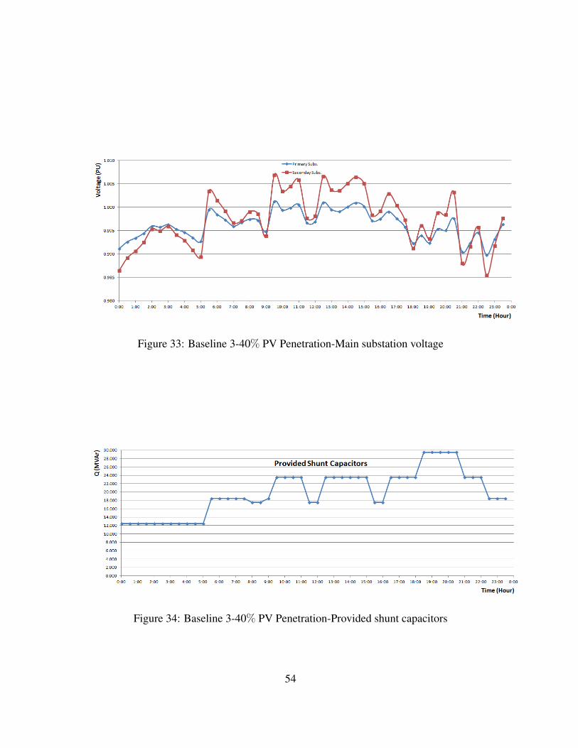
Figure 33: Baseline 3-40% PV Penetration-Main substation voltage
Figure 34: Baseline 3-40% PV Penetration-Provided shunt capacitors
54
The Q injection via the provided shunt capacitors, which are installed at 102, 106,
203, and 206 service buses, is exactly the same as the previous two baselines (baseline 1
and 2), starts with 12.5 MVAr and ends with 18.5 MVAr with identical steps as mentioned
(2 fixed capacitors, 4.5 and 3.0 MVAr at 106 and 206 service buses respectively, and 2
discrete capacitors, 12.0 and 10.0 MVAr at 102 and 203 service buses in 2 equally steps
each). The main purpose of the shunt capacitors is to compensate the drop in voltage
profile and they are considered as the simplest and inexpensive way for the power factor
correction.
In contrast with the provided reactive power through the shunt capacitors, the volt-
age profile for each bus in the system (utilization, service, and main substation buses) lies
within the specified operating range compared with the previous baselines (1 and 2). For
utilization and service buses, the minimum voltage magnitude occurred 9:00 PM while
for the main substation (primary and secondary) is at 10:30 PM. The maximum reached
point of operation to the voltage profile for the utilization, service, main substation buses
occurred at 9:30 AM.
The voltage profile for the main substation lies from 0.985 to a little more than
1.00 PU. The voltage profiles for the service buses range from approximately 0.94 to
1.04 PU, right on the edge compared with the reference standard. The voltage profiles
for the utilization buses ranges from 0.925 to almost 1.025 PU. As a result, the voltage
profile for each bus in the system (utilization, service, and main substation ”primary and
secondary” buses) is within the specified limit of operation and therefore, the distribution
system works well in the intended manner of voltage stability.
55
4.4 Baseline 4: 0.95 PF WRT SPV
In this baseline, the capability of the used inverter is sized to be 105% of the max-
imum active power produced from the PV module, that is; the reactive power capability is
increased from zero to nearly 32% at the maximum PV power generation condition as in
baseline 3 except that the inverter topology for providing a reactive power component to
the grid is directly proportional to the apparent power of the inverter. This means that the
inverter has the ability provide/absorb the reactive power component with a power factor
ranges from unity to 0.95 leading/lagging (the inverter can behave as both an inductor
”absorb a reactive power component” and a capacitor ”provide a reactive power compo-
nent” upon the required voltage profile). The Q capacity during no sun condition for the
inverter is then 105% (because Q is proportional to the inverter’s apparent power).
4.4.1 40% PV Penetration
Herein, 40% of PV penetration with respect to the maximum load is 6.023 MVA
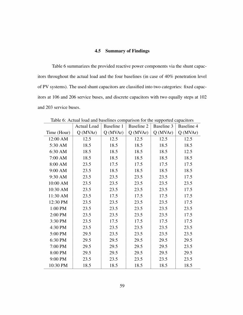
(40% x 15.058 MVA). Fig. 35, through Fig. 37, illustrate the voltage regulation behavior
for each bus in the distribution system (utilization, service, and main substation buses)
during different intervals of time (every 30 minutes). Each figure demonstrates the steady
state voltage profile behavior for the specified buses upon the distribution system bus type.
Fig. 38, illustrate the shunt capacitors provided by the system during different intervals of
time (every half an hour). The shunt capacitors are installed in four service buses (at 102,
106, 203, and 206 buses) whereas the PV systems are located on four utilization buses
(1002, 1004, 1006, and 1008 buses) in equally magnitude.
56
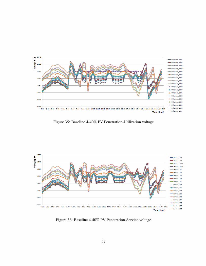
Figure 35: Baseline 4-40% PV Penetration-Utilization voltage
Figure 36: Baseline 4-40% PV Penetration-Service voltage
57
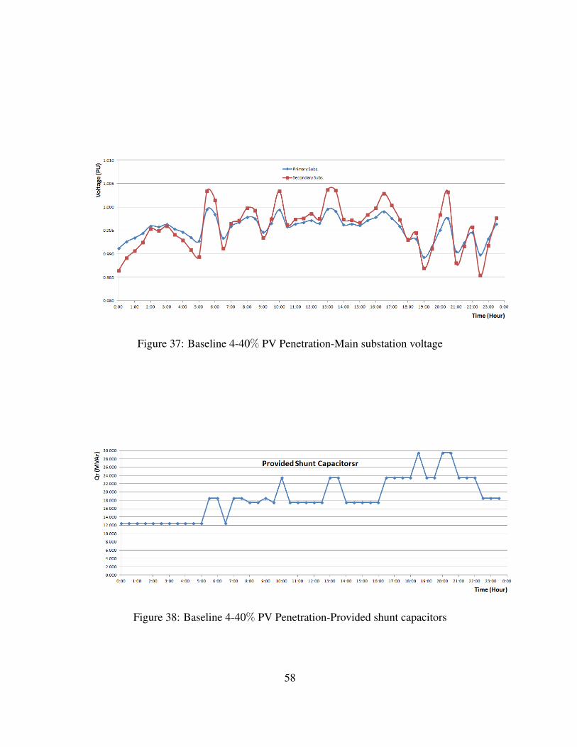
Figure 37: Baseline 4-40% PV Penetration-Main substation voltage
Figure 38: Baseline 4-40% PV Penetration-Provided shunt capacitors
58
4.5 Summary of Findings
Table 6 summarizes the provided reactive power components via the shunt capac-
itors throughout the actual load and the four baselines (in case of 40% penetration level
of PV systems). The used shunt capacitors are classified into two categories: fixed capac-
itors at 106 and 206 service buses, and discrete capacitors with two equally steps at 102
and 203 service buses.
Table 6: Actual load and baselines comparison for the supported capacitorsActual Load Baseline 1 Baseline 2 Baseline 3 Baseline 4
Time (Hour) Q (MVAr) Q (MVAr) Q (MVAr) Q (MVAr) Q (MVAr)12:00 AM 12.5 12.5 12.5 12.5 12.55:30 AM 18.5 18.5 18.5 18.5 18.56:30 AM 18.5 18.5 18.5 18.5 12.57:00 AM 18.5 18.5 18.5 18.5 18.58:00 AM 23.5 17.5 17.5 17.5 17.59:00 AM 23.5 18.5 18.5 18.5 18.59:30 AM 23.5 23.5 23.5 23.5 17.510:00 AM 23.5 23.5 23.5 23.5 23.510:30 AM 23.5 23.5 23.5 23.5 17.511:30 AM 23.5 17.5 17.5 17.5 17.512:30 PM 23.5 23.5 23.5 23.5 17.51:00 PM 23.5 23.5 23.5 23.5 23.52:00 PM 23.5 23.5 23.5 23.5 17.53:30 PM 23.5 17.5 17.5 17.5 17.54:30 PM 23.5 23.5 23.5 23.5 23.55:00 PM 29.5 23.5 23.5 23.5 23.56:30 PM 29.5 29.5 29.5 29.5 29.57:00 PM 29.5 29.5 29.5 29.5 23.58:00 PM 29.5 29.5 29.5 29.5 29.59:00 PM 23.5 23.5 23.5 23.5 23.5
10:30 PM 18.5 18.5 18.5 18.5 18.5
59
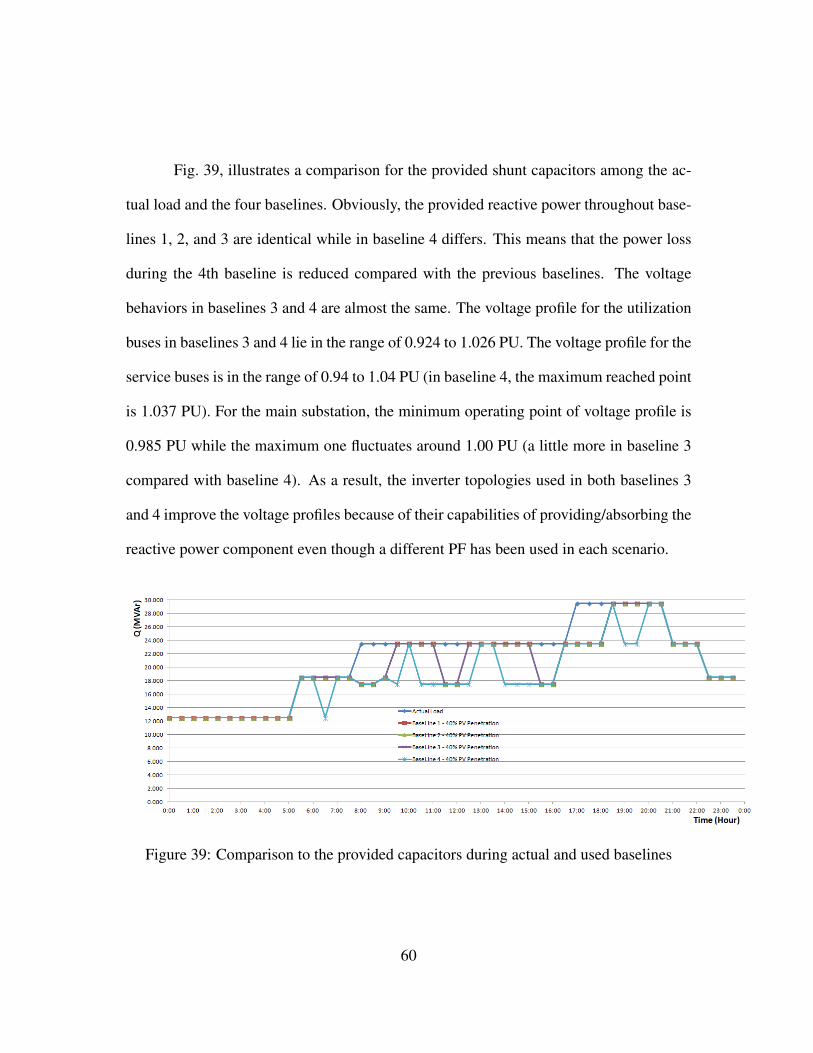
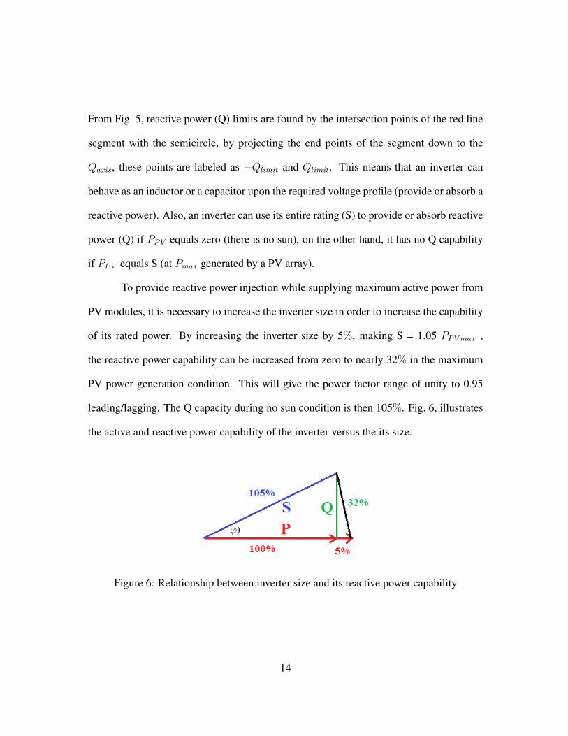
Fig. 39, illustrates a comparison for the provided shunt capacitors among the ac-
tual load and the four baselines. Obviously, the provided reactive power throughout base-
lines 1, 2, and 3 are identical while in baseline 4 differs. This means that the power loss
during the 4th baseline is reduced compared with the previous baselines. The voltage
behaviors in baselines 3 and 4 are almost the same. The voltage profile for the utilization
buses in baselines 3 and 4 lie in the range of 0.924 to 1.026 PU. The voltage profile for the
service buses is in the range of 0.94 to 1.04 PU (in baseline 4, the maximum reached point
is 1.037 PU). For the main substation, the minimum operating point of voltage profile is
0.985 PU while the maximum one fluctuates around 1.00 PU (a little more in baseline 3
compared with baseline 4). As a result, the inverter topologies used in both baselines 3
and 4 improve the voltage profiles because of their capabilities of providing/absorbing the
reactive power component even though a different PF has been used in each scenario.
Figure 39: Comparison to the provided capacitors during actual and used baselines
60
CHAPTER 5
CONCLUSIONS AND RECOMMENDATIONS
5.1 Conclusions
In this thesis, a representative distribution system arrangement was selected from
a NREL study [6]. The selected network includes voltage control equipment such as on-
load tap-changing transformer and switched capacitors. The model was further modified
and expanded to represent service transformers and secondary circuits (end-user and most
likely the point of the PV inverter connection). The selected distribution system was
modeled using PowerWorld Simulator 15 GSO after considering the major assumptions
were described in chapter 3. The network was used for analyzing the impact of different
penetrations of PV on the voltage profiles for each bus in the system. Four baselines
were used upon different inverter topology and penetration scenarios of PV levels. The
following summarizes the conclusions of this study:
• The study results show that the level of PV penetration depends on the feeder load
profile, the inverter power factor capability, and the voltage operating points.
• The studies have shown that the level of penetration upto 20% is acceptable.
• The rule of thumb of maximum of 15% penetration is not valid assumption and the
actual penetration level dependent in the individual feeder load profile, the inverter
reactive power capability, and the voltage operating points.
61
5.2 Recommendations
With respect to reactive power supply to the system, PV inverters are disadvan-
taged because their capabilities of reactive power injections are limited by either apparent
or generated active power from PV units. This can be resolved by coordinated control
of utility equipment and inverters, also, the inverters reactive power capabilities might
be needed during no sun conditions to improve the voltage profiles at some buses. This
study illustrates several such cases, inveter topologies and PV penetration levels, but it
is limited to one distribution feeder, a more comprehensive coverage of feeder profiles
would be beneficial. Islanding refers to the condition of a DG generator that continues
to feed the circuit with power, even after power from the electric utility grid has been
cut off. Distributed generators must detect islanding and immediately stop feeding the
utility lines with power, this is known as anti-islanding. The following summarizes the
recommendations for future work in this field:
• Extend to include more feeder, load, and PV profiles, so that better rule of thumbs
based on feeder loads and impedances can be formed without a detailed impact
study can be formed.
• This study only considered the steady state performance of PV systems; the dy-
namic performance of PV system such as: frequency regulation, dynamic voltage
regulation, short circuit current calculations, and anti-islanding also to be consid-
ered in the future work.
62
REFERENCE LIST
[1] H. L. Willis, “Power Distribution Planning Reference Book,” CRC Press, 2010.
[2] S. Kann, S. Mehta, M. Shiao, A. Krulewitz, C. Campbell, S. Burger, N. Litvak,
J. Baca, W. Lent, and S. Rumery, “US Solar Market Insight Report - 2012 Year in
Review - Executive Summary,” Technical Report, SEIA/GTM Research, 2013.
[3] E. Liu and J. Bebic, “Distribution System Voltage Performance Analysis for High-
Penetration Photovoltaics,” Subcontract Report, NREL/SR-581-42298, February
2008.
[4] A. Hoke, R. B. J. Hambrick, and B. Kroposki, “Maximum Photovoltaic Penetration
Levels on Typical Distribution Feeders,” Journal Article, NREL/JA-5500-55094,
July 2012.
[5] P. Kundur, J. Paserba, V. Ajjarapu, G. Andersson, A. Bose, C. Canizares, N. Hatziar-
gyriou, D. Hill, A. Stankovic, and C. Taylor, “Definition and Classification of Power
System Stability: IEEE/CIGRE Joint Task Force on Stability Terms and Defini-
tions,” IEEE Transactions on Power Systems, Vol. 19, No. 2, PP. 1387-1401, IEEE,
May 2004.
[6] Z. Ye, R. Walling, N. Miller, P. Du, K. Nelson, L. Li, R. Zhou, L. Garces, and
M. Dame, “Reliable, Low-Cost Distributed Generator/Utility System Interconnect,”
Subcontract Report, NREL/SR-560-38017, March 2006.
63
[7] T. A. Short, “Electric Power Distribution Handbook,” CRC Press, 2003.
[8] S. Repo, H. Laaksonen, P. Jarventausta, O. Huhtala, and M. Mickelsson, “A Case
Study of a Voltage Rise Problem due to a Large Amount of Distributed Genera-
tion on a Weak Distribution Network,” 2003 IEEE Bologna Power Tech Conference
Proceedings, Vol. 4, PP. 6, IEEE, 2003.
[9] T. Basso and R. DeBlasio, “IEEE Smart Grid Series of Standards IEEE 2030 (Inter-
operability) and IEEE 1547 (Interconnection) Status,” Conference Paper, NREL/CP-
5500-53028, April 2012.
[10] C. Schauder, “Impact of FERC 661-A and IEEE 1547 on Photovoltaic Inverter De-
sign,” 2011 IEEE Power and Energy Society General Meeting, PP. 1-6, IEEE, 2011.
[11] M. Abdel-Salam, “High-Voltage Engineering: Theory and Practice, Revised and
Expanded,” CRC Press, 2000.
[12] W. Kramer, S. Chakraborty, B. Kroposki, and H. Thomas, “Advanced Power Elec-
tronic Interfaces for Distributed Energy Systems,” Technical Report, NREL/TP-581-
42672, March 2008.
[13] N. G. Hingorani, L. Gyugyi, and M. El-Hawary, “Understanding Facts: Concepts
and Technology of Flexible AC Transmission Systems,” Vol. 1, IEEE Press New
York, 2000.
[14] R. Billinton, R. N. Allan, and R. N. Allan, “Reliability Evaluation of Power Sys-
tems,” Vol. 2, Plenum Press New York, 1984.
64
[15] P. Hersch and K. Zweibel, “Basic Photovoltaic Principles and Methods,” Technical
Report, Solar Energy Research Inst., 1982.
[16] M. Alam, K. Muttaqi, and D. Sutanto, “Distributed Energy Storage for Mitigation
of Voltage-Rise Impact caused by Rooftop Solar PV,” 2012 IEEE Power and Energy
Society General Meeting, PP. 1-8, IEEE, 2012.
[17] F. Blaabjerg and E. Koutroulis, “Methods for the Optimal Design of Grid-Connected
PV Inverters,” International Journal of Renewable Energy Research, Vol. 1, No. 2,
PP. 54-64, IJRER, 2011.
[18] T. Van Cutsem and C. Vournas, “Voltage Stability of Electric Power Systems,” Vol.
441, Springer, 1998.
[19] W. C. Sealey, “Distribution Voltage Regulator,” US Patent 3,041,560, June 1962.
[20] P. P. Barker and R. W. De Mello, “Determining the Impact of Distributed Generation
on Power Systems. I. Radial Distribution Systems,” 2000 IEEE Power Engineering
Society Summer Meeting, Vol. 3, PP. 1645-1656, IEEE, 2000.
[21] L. Kojovic, “Impact of DG and Voltage Regulator Interaction on Distribution System
Voltage Regulation,” International Conference on Electricity Distribution, 2003.
[22] H. Jimenez, H. Calleja, R. Gonzalez, J. Huacuz, and J. Lagunas, “The Impact of
Photovoltaic Systems on Distribution Transformer: A C ase Study,” Energy Conver-
sion and Management, Vol. 47, No. 4, PP. 311-321, Elsevier, 2006.
VITA
I, Abdulsalam Elsaidi was born on September 4, 1976 in Sirte, Libya.
I was educated in local public schools and got the first diploma in instrumentation
major from PTQI (Petroleum Training and Qualifying Institute) in 1994, Tripoli-Libya.
I have obtained my B.Sc. degree from Al-Tahadi University, automatic control and in-
strumentation major in 1999 at the ripe age of 23. I have worked for GECOL (General
Electrical Company of Libya) 10 years (June 2000 - Mach 2010) in distribution field, a
head of laboratory and measurement department, Sirte State. At the time of writing this
vita, I am supposed to get my MS degree.
66