1

Pennsylvania Climate Impacts Assessment Update

May 2015

James Shortle1 (PI), Professor

David Abler1 (Co-PI), Professor Seth Blumsack2 Assistant Professor

Aliana Britson6 Post Doctoral Scholar Kuai Fang5 Graduate Student

Armen Kemanian7 Assistant Professor Paul Knight4 Sr. Lecturer

Marc McDill3 (Co-PI), Associate Professor Raymond Najjar4 Professor

Michael Nassry6 Post Doctoral Scholar Richard Ready1 (Co-PI), Associate Professor

Andrew Ross4 Graduate Student Matthew Rydzik4Graduate Student Chaopeng Shen5 Assistant Professor

Shilong Wang5 Graduate Student Denice Wardrop6 Senior Scientist Susan Yetter8 Research Assistant

1Agricultural Economics, Sociology, and Education 2Energy and Mineral Engineering

3School of Forest Resources 4Meteorology

5Civil and Environmental Engineering 6Geography

7Plant Science 8Riparia

The Pennsylvania State University, University Park

For correspondence about this report, contact James Shortle at 814-865-8270, or jshortle@psu.edu

2

Table of Contents Contributors ............................................................................................................................................ 5

Executive Summary ................................................................................................................................. 6

Pennsylvania Climate Futures ............................................................................................................ 6

Sectoral Assessments .......................................................................................................................... 7

Agriculture ........................................................................................................................................... 7

Energy .................................................................................................................................................. 8

Forests .................................................................................................................................................. 9

Human Health .................................................................................................................................... 10

Outdoor Recreation ........................................................................................................................... 11

Water .................................................................................................................................................. 12

Wetlands and Aquatic Ecosystems .................................................................................................. 13

Coastal Resources ............................................................................................................................... 14

1 Introduction .................................................................................................................................... 15

1.1 Background ................................................................................................................................ 15

1.2 Methodology Overview ............................................................................................................. 15

References .......................................................................................................................................... 17

2 Past and future climate of Pennsylvania ...................................................................................... 18

2.1 Introduction ............................................................................................................................... 18

2.2 Sources of observational data and climate simulations ............................................................ 18

2.3 Data processing and analysis ..................................................................................................... 25

2.4 Historical climate ....................................................................................................................... 27

2.4.2 Potential causes of changes .................................................................................................... 35

2.5 Climate projections .................................................................................................................... 41

2.6 Summary .................................................................................................................................... 56

Appendix A ......................................................................................................................................... 58

References .......................................................................................................................................... 60

Abbreviations .................................................................................................................................... 62

Acknowledgements ........................................................................................................................... 62

3 Agriculture ...................................................................................................................................... 63

3.1 Introduction ............................................................................................................................... 63

3.2 Present-day Pennsylvania agriculture ....................................................................................... 64

3

3.3 Economic and policy scenarios .................................................................................................. 66

3.4 Climate change impacts ............................................................................................................. 72

3.5 Economic opportunities and barriers for Pennsylvania ............................................................ 86

3.6 Conclusions ................................................................................................................................ 88

References .......................................................................................................................................... 89

4 Energy Impacts of Pennsylvania’s Climate Futures .................................................................... 94

4.1 Introduction ............................................................................................................................... 94

4.2 Pennsylvania’s Energy Sector .................................................................................................... 94

4.3 Greenhouse-gas impacts of energy production and consumption in Pennsylvania ................. 98

4.4 Climate change is likely to increase overall energy demand in Pennsylvania ......................... 101

4.5 Climate Change and the Reliability of Energy Delivery............................................................ 106

4.6 Uncertainties and Opportunities for Pennsylvania’s Energy Sector ........................................ 111

4.7 Conclusions .............................................................................................................................. 112

References ........................................................................................................................................ 113

5 Forest Resources .......................................................................................................................... 114

5.1 Introduction ............................................................................................................................. 114

5.2 Projected climate change impacts .............................................................................................. 115

5.3 Mitigation and adaptation .......................................................................................................... 121

5.4 Forest management opportunities related to climate change................................................ 123

5.5 Forest management barriers related to climate change ......................................................... 123

References ........................................................................................................................................ 124

6 Human Health Impacts ................................................................................................................. 131

6.1 Introduction ............................................................................................................................. 131

6.2 Air Quality ................................................................................................................................ 132

6.3 Water Quality ........................................................................................................................... 133

6.4 Extreme Weather Events ......................................................................................................... 134

6.5 Vector-borne Disease .............................................................................................................. 135

6.6 Airborne Infectious Disease ..................................................................................................... 136

6.7 Adaptation Opportunities and Barriers ................................................................................... 137

References ........................................................................................................................................ 137

7 Outdoor Recreation ....................................................................................................................... 141

7.1 Introduction ............................................................................................................................. 141

4

7.2 National Estimates of Changes in Outdoor Recreation ........................................................... 141

7.3 Winter Recreation .................................................................................................................... 143

7.4 Recreational Fishing ................................................................................................................. 145

7.5 Water-Based Recreation .......................................................................................................... 148

7.6 Outdoor Sports and Exercise Activities .................................................................................... 148

7.7 Adaptation Opportunities and Barriers ................................................................................... 149

References ........................................................................................................................................ 150

8 Water Resources ........................................................................................................................... 152

8.1 Introduction ............................................................................................................................. 152

8.2 Basic hydrologic characteristics of Pennsylvania basins .......................................................... 153

8.3 Data-based assessment of climate change impacts in the past decade ................................. 155

8.4 Future climate change trends and adaptation ..................................................................... 167

8.5 Information needs .................................................................................................................. 169

Appendix .......................................................................................................................................... 170

References ........................................................................................................................................ 171

9 Wetlands ........................................................................................................................................ 174

9.1 Introduction ............................................................................................................................. 174

9.2 Definition and Description of Ecosystem Services................................................................... 175

9.3 Vulnerability of Wetlands, Streams, Lakes, and Rivers to Climate Change Effects ................. 176

9.4 Vulnerability of Pennsylvania Watersheds and Wetlands to Climate Change Impacts .......... 182

9.5 Conclusions and Recommendations ........................................................................................ 191

References ........................................................................................................................................ 191

10 Coastal resources ........................................................................................................................ 197

10.1 Potential impact of climate change on southeastern Pennsylvania’s coastal resources ...... 197

References ........................................................................................................................................ 198

5

Contributors This report is the result of the collective work of the contributors. Lead authors and contributors for the components of the report are: Past and Future Climate of Pennsylvania

Raymond Najjar, Professor of Oceanography, Joint Appointment in the Departments of Geosciences and Meteorology

Paul Knight, Senior Lecturer in Meteorology, Weather World Host, Pennsylvania State Climatologist, Department of Meteorology

Research Assistants: Andrew Ross, Justin Schulte, Kyle Imhoff Agriculture

David Abler, Professor of Agricultural, Environmental and Regional Economics and Demography, Department of Agricultural Economics, Sociology, and Education

Armen Kemanian, Assistant Professor of Production Systems and Modeling, Department of Plant Science Energy

Seth Blumsack, Associate Professor of Energy Policy and Economics, John and Willie Leone Family Department of Energy and Mining Engineering

Forests

Marc McDill, Associate Professor of Forest Management, Department of Ecosystem Science and Management

Human Health, Recreation, and Tourism

Richard Ready, Professor of Agricultural and Environmental Economics, Department of Agricultural Economics, Sociology, and Education

Water Resources

Chaopeng Shen, Assistant Professor of Civil Engineering, Department of Civil and Environmental Engineering

Research Assistants: Kuai Fang, Shilong Wang Wetlands and Aquatic Ecosystems

Denice Wardrop, Senior Scientist and Professor of Ecology and Geography, Department of Geography, and Director, Penn State’s Sustainability Institute

Michael Nassry, Post Doctoral Scholar, Department of Geography and Riparia Aliana Britson, Post Doctoral Scholar, Department of Geography and Riparia Susan Yetter, Research Assistant, Riparia

6

Executive Summary The Pennsylvania Climate Change Act (PCCA), Act 70 of 2008 directed Pennsylvania’s Department of Environmental Protection (DEP) to conduct a study of the potential impacts of global climate change on Pennsylvania over the next century. This study was conducted for DEP by a team of scientists at The Pennsylvania State University and presented in the two reports: Pennsylvania Climate Impacts Assessment (Shortle et al., 2009) and Economic Impacts of Projected Climate Change in Pennsylvania (Abler et al., 2009). This report is the second update of the original report by the Penn State team. The first update was prepared in 2013 (Ross et al., 2013). The purpose of the updates is to capture advances in the scientific understanding of climate change and climate change impacts, and make use of new data sets, relevant to Pennsylvania. The 2009 Pennsylvania Climate Impacts Assessment and the 2013 Pennsylvania Climate Impacts Assessment Update presented simulations of the impacts of global climate change on Pennsylvania’s climate in the 21st century. They also presented assessments of the impacts of climate change in Pennsylvania on climate sensitive sectors and the general economy. Just as the 2013 update revisited the conclusions of the 2009 study based on new scientific findings, data, and analyses that became available after the original report, this study revisits those conclusions based on new scientific findings, data, and analyses that have become available since the 2013 update.

Pennsylvania Climate Futures Data sets and analytical techniques for examining Pennsylvania’s Climate Futures have advanced significantly since the 2009 Impact Assessment and the 2013 update. Since those reports, the Intergovernmental Panel on Climate Change (IPCC) released its Fifth Assessment Report (AR5), which included new scenarios for future concentrations of greenhouse gases in the Earth’s atmosphere. The IPCC’s AR5 also ushered in the Coupled Model Intercomparison Project Phase 5 (CMIP5), providing new output from a suite of General Circulation Models running standardized simulation experiments. This update analyzes historical and future changes in Pennsylvania’s climate utilizing the new data sets, new statistical techniques, and the most recent suite of global and regional climate model simulations. The findings are largely similar to those of the 2009 Report and 2013 Update. Pennsylvania has undergone a long-term warming of more than 1 °C (1.8°F) over the past 110 years, interrupted by a brief cooling period in the mid-20th century. This pattern is simulated by climate models only when anthropogenic forcing, mainly increases in greenhouse gases, are included. However, naturally varying climate modes, specifically, the North Atlantic Oscillation, the El Niño/Southern Oscillation, the Pacific Decadal Oscillation, and the Pacific North American pattern, all influence Pennsylvania’s temperature and (especially) precipitation. The effects of climate modes on Pennsylvania’s precipitation are dominant at periods of about 20 years. Changes in Pennsylvania’s temperature are reflected in other metrics, such as heating degree days (which have increased) and cooling degree days (which have decreased). An analysis of above- and below-normal precipitation in the agriculturally productive southeastern portion of Pennsylvania shows a decreasing number of very dry months and an increasing number of very wet months, which reflects the overall wetting trend in the Commonwealth.

7

Pennsylvania’s current warming and wetting trends are expected to continue at an accelerated rate. This report adopts the Representative Concentration Pathway 8.5 (RCP 8.5). This pathway is the one that the world is currently on, and is one of two emissions pathways adopted by a large number of climate modeling groups. Under RCP 8.5 it is projected that by the middle of the 21st century, Pennsylvania will be about 3 °C (5.4°F) warmer than it was at the end of the 20th century. The corresponding annual precipitation increase is expected to be 8%, with a winter increase of 14%. The likelihood for meteorological drought is expected to decrease while months with above-normal precipitation are expected to increase. Projections regarding Pennsylvania’s hydrology are more equivocal. Runoff and soil moisture simulations show substantial differences from products based on observations. The existing models suggest modest but significant increases in annual-mean runoff and small changes in annual-mean soil moisture.

Sectoral Assessments Climate impact (vulnerability or risk) assessments conventionally focus on the direct impacts of climate change on climate-sensitive human or natural systems. The impact on (or vulnerability of, or risk to) the system depends on the climate change to which the system is exposed, the sensitivity of the system to the exposure, and the adaptation of the system to ameliorate harms or exploit opportunities. Each element of impact assessment – the climate change that occurs, the sensitivity of systems to that change, and the adaptations – are important to the outcomes. The sectoral assessments presented in this report consider exposures, sensitivities, and adaptations in assessing potential impacts. Importantly, impacts are not exclusively negative. For example, warmer, wetter environments can be beneficial for some crops, and warmer winters can reduce human health risks associated with cold weather. Accordingly, impacts are risks or vulnerabilities in many cases, but provide for opportunities in others. Impacts are uncertain for many reasons. These reasons include: (1) uncertainty about the paths of greenhouse gas emissions and global and regional climate responses to those paths result in uncertainty about climate change; (2) incomplete knowledge of the sensitivity of various systems to climate change along with incomplete knowledge and uncertainty about current and future adaptation options, their effectiveness, and their likely utilization result in uncertainty about the impacts of alternative climate futures on climate sensitive sectors; and (3) uncertainty about other stressors that may interact with climate change to determine impacts in climate sensitive sectors. Further, impacts are by definition, an assessment of what the world would be like with climate change, and attendant adaptations, and without. Considering the evolution of our world over the past 100 years, it is apparent that its evolution without climate change is subject to significant uncertainty.

Agriculture Agriculture in Pennsylvania, like agriculture in the rest of the United States and worldwide, has an intrinsic relationship with climate. Most crop and livestock production in Pennsylvania occurs partly or entirely in the open air, exposed to the elements and dependent on the weather for success. Even production that occurs under controlled climatic conditions, such as a mushroom house, is affected by climate through heating and cooling costs. Beyond direct effects of global climate change on agriculture through its effects on growing conditions in Pennsylvania, climate change can also affect the Commonwealth’s agriculture through its effects on the prices of agricultural commodities, which are determined by regional, national, and international markets that are affected by climate-induced changes in supply and demand.

8

Our analyses of recent scientific findings for this Update largely support conclusions drawn in the prior Update. Climate change and increasing atmospheric carbon dioxide (CO2) concentrations are likely to have mixed effects on Pennsylvania field crop production. Higher average temperatures and higher average precipitation projected for Pennsylvania will present both positives and negatives for field crop producers, who will also have to adapt to negatives caused by greater extremes in temperature and precipitation. The effects of climate change on Pennsylvania nursery and greenhouse production are uncertain. For example, the effects of climate change on mushroom production will primarily be manifested in changes in heating and cooling requirements for growing houses. With climate change, there will on average be less heating during the winter months but additional cooling during the summer months, with the net effect on annual energy use being unclear. Pennsylvania dairy production is likely to be negatively affected by climate change due to losses in milk yields caused by heat stress, additional energy and capital expenditures to mitigate heat stress, and lower levels of forage quality. On the other hand, forage yields may increase due to a longer growing season and more precipitation on average. As Pennsylvania is part of local, regional, national, and global markets for food and agricultural products, indirect effects of climate change on Pennsylvania agriculture caused by changes in climate in other parts of the nation and world may be significant. For example, warmer climates in southern states could stimulate a large-scale movement of poultry and hog production northward into states like Pennsylvania. Agriculture in Pennsylvania has changed dramatically since 1900 and will likely change in profound ways between now and 2100 regardless of whether climate change is large or small. Some of these changes may impact how Pennsylvania agriculture responds to climate change. For example, organic agriculture is growing a market segment that faces different vulnerabilities than non-organic agriculture to new pests and diseases in a warmer climate. Efforts to mitigate greenhouse gas emissions may create an economic opportunity for Pennsylvania agriculture in energy crop production. Candidates include perennial shrub willow (a short-rotation woody crop), the perennial grasses miscanthus and switchgrass, and annuals such as biomass sorghum or winter rye.

Energy Pennsylvania’s status as a major energy-producing state has grown over the past two years. Pennsylvania is now the third-largest energy-producing state in the U.S. (on a BTU basis), behind Texas and Wyoming. This change is almost entirely attributable to the growth in natural gas production. Our analyses of recent scientific findings for this Update largely support major conclusions drawn in the 2009 Assessment and 2013 Update.

• Warming in Pennsylvania is likely to increase demand for energy, particularly electric power, during the summer months. This increase is likely to be larger than any decline in wintertime energy consumption, implying an overall increase in energy utilization in the Commonwealth as

9

a result of climate change. Policies to reduce greenhouse gases and localized emissions are likely to increase demand for natural gas produced in Pennsylvania.

• Existing policies, such as the Alternative Energy Portfolio Standard and some aspects of Pennsylvania Act 129, have addressed opportunities for the Commonwealth to facilitate the adaptation to climate change as well as mitigation of further greenhouse gas emissions. Additional opportunities exist, particularly in the areas of low-emissions power generation, energy efficiency and demand-side management of electric energy consumption.

• Increased seasonal variations on freshwater supplies may impact the ability of Pennsylvania’s energy sector (particularly power generation facilities that require cooling water) to produce reliable supplies under some scenarios.

Several new issues have emerged since the 2013 Update.

• Declines in energy commodity prices, particularly for electricity and natural gas, will present challenges to some technology options that could contribute to climate change mitigation. Unless otherwise supported through incentive programs, the economics of renewable power generation in the Commonwealth (primarily wind and solar photovoltaics) will continue to be negatively impacted. With current market conditions, large-scale renewable energy projects in Pennsylvania face increasing costs due primarily to locational factors (for example, many of the best wind sites have already been developed).

• Recent extreme weather events have focused attention on how climate change may affect the reliability of energy delivery systems. Recent work has attempted to quantify the reliability benefits of a more distributed model of electric power production and delivery, but additional research is needed.

• Updated climate models suggest that pressures on water quantity available for the energy sector in Pennsylvania may not represent a significant energy system stressor, although the models do project some changes in seasonal variation.

Forests Forests are the dominant land use in Pennsylvania, covering 16.6 million acres or 58 percent of land area. Pennsylvania’s forests have long been subject to multiple stressors. These include exotic pests and diseases, invasive species, over-abundant deer populations, atmospheric deposition of air pollutants, unsustainable harvesting practices, and now climate change. Climate change is already radically affecting some forests around the world and, to a lesser degree, the forests of Pennsylvania. Climate change will likely continue to affect them in increasingly dramatic ways in the future. Key findings of this and previous reports are:

• Suitable habitat for tree species is expected to shift to higher latitudes and elevations. This will reduce the amount of suitable habitat in Pennsylvania for species that are at the southern extent of their range in Pennsylvania or that are found primarily at high latitudes; the amount of habitat in the state that is suitable for species that are at the northern extent of their range in Pennsylvania will increase.

• The warming climate will cause species inhabiting decreasingly suitable habitat to become stressed. Mortality rates are likely to increase and regeneration success is expected to decline for these species, resulting in declining importance of those species in the state.

10

• Longer growing seasons, higher temperatures, higher rainfall, nitrogen deposition, and increased atmospheric CO2 may increase overall forest growth rates in the state, but the increased growth rates for some species may be offset by increased mortality for others.

• The state’s forest products industry will need to adjust to a changing forest resource. The industry could benefit from planting faster-growing species and from salvaging dying stands of trees. Substantial investments in artificial regeneration may be needed if large areas of forests begin to die back due to climate-related stress.

• Forests can contribute to the mitigation of climate change by sequestering carbon. It would be difficult to substantially increase the growth rates of Pennsylvania hardwoods, however, so the best opportunities most likely lie in preventing forest loss.

• Forests can be a significant source of biomass to replace fossil fuels.

Forest carbon management can help ameliorate the rate and amount of climate change. Forests represent one of the significant pools of terrestrial carbon. The size of this pool can be increased through forest management, primarily by increasing stand densities, increasing rotation lengths, and reducing mortality. Furthermore, removal rates from this pool can be moderated by reducing conversion of forests to non-forest land uses. One option for mitigating climate change through forest management is by substituting fossil fuels with wood in the production of energy. Using wood biomass for energy is controversial as it will generally result in increased emissions in the short run. The length of time it takes to achieve net carbon benefits is highly variable, ranging from a few years to more than a century. Climate change is already occurring and will continue, albeit at different rates, under all emissions scenarios. Because climate change is also inevitable, forests must be managed to increase their resiliency in the face of climate change. To accomplish this, non-climate threats to forest health and diversity, including insect pests, diseases, invasive plants and animals, overabundant deer populations, unsustainable harvest practices, and atmospheric deposition, must also be addressed. The primary forest management opportunities related to climate change are: 1) carbon trading, 2) increased markets for low-use wood for energy production, and 3) potentially renewed interest and will to manage forests for their long-term health and resiliency. The primary barriers to managing Pennsylvania’s forests for health and resiliency in the face of climate change are: 1) lack of knowledge, 2) the complexity of influencing the management practices of more than half a million private forest landowners, and 3) the host of confounding, interrelated challenges to managing forests for diversity, health and resiliency.

Human Health Climate change has the potential to affect human health through several different mechanisms. For each mechanism, however, there are opportunities to reduce the potential impact on human health. This report reviews recent research findings on the potential impacts of climate change on human health that are relevant to Pennsylvania. Higher temperatures will increase mortality from heat-related stress, but will decrease mortality from cold-related stress. While each of these effects is predicted with high confidence, the net effect on total mortality is unclear. However, the mortality risk from extreme heat events has been falling, as more and more households install air conditioning.

11

Climate change will worsen air quality relative to what it would otherwise be, causing increased respiratory and cardiac illness. The linkage between climate change and air quality is most strongly established for ground-level ozone creation during summer, but there is some evidence that higher temperatures and higher precipitation will result in increased allergen (pollen and mold) levels as well. The predicted impact of climate change on particulate concentrations is not clearly established. Air quality impacts from climate change are due to the combination of pollutants emitted from human sources and weather conditions. The most important adaptation strategy to reduce human health impacts from air quality changes due to climate change is to reduce pollutant emissions, particularly volatile organic compounds and nitrogen and sulfur oxides from combustion. Climate change can potentially also worsen water quality, affecting health through drinking water and through contact during outdoor recreation. The two primary mechanisms through which climate change could affect surface water quality are 1) increased pathogen loads due to increased surface runoff from livestock farms, sewer overflows, and resuspension of pathogens in river sediments during heavy rainstorms, and 2) increased risk of harmful algal blooms in eutrophied lakes and reservoirs. As with air quality, human health impacts from compromised water quality are due to the combination of pollutant emissions and weather. The most important adaptation strategy to reduce human health impacts from water quality changes due to climate change is to reduce nutrient and pathogen loadings to rivers and streams. The risk of injury and death from extreme weather events could increase as a consequence of climate change. There is a consensus in the literature that climate change will not necessarily increase the number of tropical cyclones, but that it will increase the probability that individual storms will be stronger and with heavier rainfall. Non-tropical extreme rainfall events are expected to increase as a consequence of climate change. The most important adaptation strategies to reduce injury and death from increased extreme weather due to climate change are to build homes and infrastructure in ways to minimize the risk to them from flooding, and to invest in storm forecasting and notification systems. Climate change could affect the distribution and prevalence of vector-borne diseases such as Lyme Disease and West Nile Virus. However, there is no clear consensus on whether climate change would increase or decrease risk of these diseases in Pennsylvania. Climate change could also affect the prevalence and virulence of air-borne infectious diseases such as influenza. However, again, there is no clear consensus on whether climate change would increase or decrease ill health from these diseases in Pennsylvania. For both vector-borne diseases and air-borne infectious disease, the most effective adaptation strategy to minimize the risk to human health is to assure that Pennsylvania residents have access to health care services.

Outdoor Recreation By its nature, outdoor recreation is sensitive to climate. With the exception of snow- and ice-based recreation, there is not clear evidence that climate change will greatly affect outdoor recreation participation. However, climate change may affect the types of recreation people choose to pursue in each season. This report reviews recent research findings on the potential impacts of climate change on outdoor recreation participation that are relevant to Pennsylvania. Climate change will have a severe, negative impact on winter recreation. Pennsylvania’s downhill ski and snowboard resorts are not expected to remain economically viable past mid-century. Snow cover to support cross country skiing and snowmobiling has been declining in Pennsylvania, and is expected to

12

further decline by 20-60%, with greater percentage decreases in southeastern Pennsylvania, and smaller decreases in northern Pennsylvania. Climate change is not expected to greatly affect the rate of participation in recreational fishing. However, it will affect the types of fishing undertaken. Some areas that currently support cold-water (trout) fishing will no longer support that type of fishery. The impact of climate change on trout fishing is expected to be particularly severe in southeastern and northwestern Pennsylvania. An important adaptation strategy to minimize the effect of climate change on trout fishing is to reduce other stressors to trout, such as nutrient and sediment loadings to streams and degradation of riparian corridors. Climate change will increase summer temperatures and increase the duration of the warm season, which will potentially increase demand for water-based recreation (swimming, canoeing, kayaking, motor-boating). However, a study of national recreation participation did not show a strong relationship between climate and participation in water-based recreation, so whatever impact that climate change may have on water-based recreation is likely to be small. Finally, general outdoor leisure activity (e.g., walking, biking, golf, tennis) is sensitive to climate. Research has shown that people spend more time in outdoor leisure activity as temperature increases. Time spent in outdoor leisure is highest when temperatures are between 75 degrees F and 100 degrees F, and only drops when daytime high temperatures exceed 100 degrees F. However, Pennsylvania cities are expected to see increases in the frequency of 100+ degree days as a consequence of climate change. The net effect of climate change on outdoor leisure is therefore an increase in activity during the spring and fall and a decrease on the hottest days of summer. Outdoor recreation of all types is expected to increase in Pennsylvania due to increasing population and income. The primary adaptation strategy for winter sports enthusiasts will be to travel longer distances to reach areas with climates that support their activities. For outdoor recreation within Pennsylvania, agencies should plan to accommodate increased demand. Outdoor recreation is sensitive to climate, but also to the quality of the recreation resource. Improved water quality will encourage increased water-based recreation, while improved air quality will allow people to participate in outdoor leisure activities in hotter weather.

Water Like the Climate Futures assessment, the water assessment in this Update benefits from the use of new data to examine trends in major components of the hydrologic cycle in Pennsylvania. Consistent with the prior assessment and update, climate change is expected to bring increased flood risks. However, in contrast to the prior assessment, new evidence indicates a strong capacity for water storage to recover from droughts in the state, mitigating concerns for low flows in the summer and significant capacity to recover from short-term droughts. Summer stream temperature records showed mixed trends in different parts of the state, but winter stream temperature showed warming trends, leading to complex outcomes that can be both opportunities and hazards for fish communities. Soil moisture trends were generally very mild. Higher peak flows have contributed to more prominent bank and soil erosion problems in the state, which have been corroborated by studies of river bed elevation trends. Combining the findings from our data-based studies and IPCC reports, we make the following statements regarding climate change impacts and adaptation for PA water resources, in addition to the actions recommended in the last impact update:

13

• ‘Low-regret’ adaptation methods that reduce vulnerability and exposure to present climate

variability with co-benefits, are promising methods to create resilience under uncertain hydrological changes. Examples of these strategies include less impervious surface, green infrastructure, rooftop gardens and conservation of wetlands.

• The impacts of droughts are likely to be short-term in Pennsylvania. However there are risks associated with short-term disasters, e.g., wetlands degradation and competition for water resources in low-flow, high-temperature periods between different sectors. Water availability issues for vulnerable communities may exist due to socio-economic inequalities.

• There are substantial and increasing flooding risks in Pennsylvania for both urban areas and infrastructure in rural areas. Adaptation strategies that focus on increasing flood preparedness, reducing vulnerabilities and increasing resilience in more extreme and more frequent flooding scenarios are of high priority. It is important to consider differential risks and vulnerabilities in adaptation strategies.

• The state should initiate programs for monitoring, assessing, estimating and abating stream bank erosion to protect overall stream health.

Wetlands and Aquatic Ecosystems This Update presents new original research on the vulnerability of Pennsylvania’s wetlands to climate change. Because the hydrological regime is the driver of aquatic ecosystem processes most directly affected by climate change, vulnerability is articulated through changes in hydrologic regime, explicitly as wetter/stable/drier conditions. The analysis of hydrologic conditions was conducted in seven watersheds selected to be representative of a range of ecoregions and predominant land cover types. For a moderate greenhouse gas emissions growth scenario, watershed-wide hydrologic conditions at mid-century are predicted to remain relatively stable on an annual basis, but show considerable change on a seasonal basis. On an annual basis, 11% of the approximately 2400 km2 in the seven modeled Pennsylvania watersheds experienced drier conditions, 37% of the area was wetter, and the remaining 51% remained stable. These values changed significantly when considering a seasonal instead of an annual basis. For example, during the winter (December, January, February), 61% of the modeled land experienced wetter conditions and 32% remained stable. Conversely, during the summer (June, July, August) 70% of the modeled land was drier, with only 19% remaining stable. The relative vulnerability of wetlands on various land cover regimes (as a proxy for condition) was also examined, with the majority of wetland acreage in forested land cover, followed by agriculture and developed land. The distribution of wetland acreage across these land cover types varies considerably by ecoregion. The majority of wetland acreage in both forested and agricultural settings is projected to remain stable or become wetter. All of the wetland acres within the developed land-use regime were in the Ridge and Valley ecoregion, and all were projected to remain stable. Only the Ridge and Valley ecoregion had any wetland acreage projected to become drier (in both forested and agricultural settings), though the majority of wetland acreage was still projected to remain stable within this ecoregion. In both the Glaciated Plateau and the Piedmont, more wetland acreage was projected to become wetter than to remain stable, while in the Unglaciated Plateau, all wetland acreage within agricultural land-use regimes was projected to remain stable. These results suggest that management action taken to protect wetlands within agricultural areas from the effects of climate change should be targeted in the Ridge and Valley ecoregion, as this was the only

14

ecoregion that had any wetland acreage projected to become drier, and also in the Glaciated Plateau, as the vast majority of wetland acreage was projected to become wetter. The majority of wetland acreage in the seven watersheds is classified as riverine or slope headwater floodplain; while almost equal percentages of wetter and stable conditions occur across this combined acreage, the results vary considerably by wetland type and ecoregion. The majority of riverine wetlands occur in the Ridge and Valley, and most of these remain stable; while the majority of slope headwater floodplains occur in the Glaciated Plateau and are projected to become wetter. Because of their direct connection to the bodies of water that people use for drinking water and recreation, riverine, slope/headwater floodplains, and slope/riparian depression wetlands are often targeted for protection and restoration. While the majority of wetland acreage for these three wetland types is projected to remain stable across most ecoregions, some riverine and slope headwater wetlands in the Ridge and Valley may become drier. Thus any management efforts to protect wetlands from the effects of climate change should be focused on these wetlands so that they are able to continue providing water quality services to nearby water-bodies.

Coastal Resources Climate change poses a threat to the fauna of the tidal freshwater portion of the Delaware estuary. One reason is that increased water temperatures with climate change decrease the solubility of oxygen in water and will increase respiration rates, both of which will result in declines in dissolved oxygen concentration. Thus climate change will worsen the currently substandard water quality in the tidal freshwater region of the Delaware Estuary. The second reason that climate change threatens tidal freshwater fauna is through salt intrusion associated with sea-level rise and summertime streamflow declines. Existing research suggests a modest impact of climate change on salinity of the upper Delaware Estuary. The freshwater tidal wetlands along Pennsylvania’s southeastern coast are a rare, diverse, and ecologically important resource. Climate change poses a threat to these wetlands because of salinity intrusion and sea-level rise. Sea-level rise, however, has the potential to drown wetlands if their accretion rates are less than rates of sea-level rise. The potential for horizontal migration is low in southeastern Pennsylvania due to extensive development. In summary, climate change has the potential to exacerbate the currently highly stressed state of Pennsylvania’s tidal wetlands.

15

1 Introduction 1.1 Background The Pennsylvania Climate Change Act (PCCA), Act 70 of 2008, directed Pennsylvania’s Department of Environmental Protection (DEP) to conduct a study of the potential impacts of global climate change on Pennsylvania over the next century. This study was prepared for DEP by a team of scientists at The Pennsylvania State University and presented to DEP in the 2009 reports: Pennsylvania Climate Impacts Assessment (Shortle et al., 2009), and Economic Impacts of Projected Climate Change in Pennsylvania (Abler et al. 2009). The PCCA required DEP to prepare updates of the Pennsylvania Climate Change Impact Assessment Report every three years to reflect advances in scientific understanding. The first update was prepared by the Penn State Team in 2013 (Ross et al., 2013). This report presents the second three year update. The 2009 Pennsylvania Climate Impacts Assessment and the 2013 Pennsylvania Climate Impacts Assessment Update presented simulations of the impacts of global climate change on Pennsylvania’s climate in the 21st century. They also presented assessments of the impacts of climate change in Pennsylvania on climate-sensitive sectors and the general economy. Just as the 2013 update revisited the conclusions of the 2009 study based on new scientific findings, data, and analyses that became available after the original report, this study revisits those conclusions based on new scientific findings, data, and analyses that have become available since the 2013 update. 1.2 Methodology Overview The general methodology underlying this work is discussed in depth in the Pennsylvania Climate Impacts Assessment (Shortle et al., 2009). A brief review of the general methods is presented below. Specific methods used in the climate futures and sector assessments are described in those sections.

1.2.1 Climate Futures An essential task for this update is to characterize Pennsylvania’s Climate Future. One approach would be to attempt to predict the actual evolution of the Commonwealth’s climate. However, climate predictions of this type are not the norm in climate change impact assessments because of the large uncertainties about the future course of greenhouse gas emissions and other factors that drive global climate change, about the response of regional climates to global climate change, and about the course of regional drivers of regional climate (e.g., land cover). Instead, the norm is to use climate change scenarios in which future climates are projected based on assumptions about the path of greenhouse gases and other determinants of climate change. Accordingly, as in the prior reports, the assessment of Pennsylvania’s Climate Futures makes use of simulations derived from a suite of General Circulation Models (GCMs) (complex mathematical models that are solved on supercomputers to simulate the earth’s climate). Data sets and analytical techniques for examining Pennsylvania’s Climate Futures have advanced significantly since the 2009 Impact Assessment and the 2013 update. Since those reports, the Intergovernmental Panel on Climate Change (IPCC) released its Fifth Assessment Report (AR5), which included new scenarios for future concentrations of greenhouse gases in the Earth’s atmosphere. The IPCC’s AR5 also ushered in the Coupled Model Intercomparison Project Phase 5 (CMIP5), providing new

16

output from a suite of General Circulation Models running standardized simulation experiments. This Update analyzes historical and future changes in Pennsylvania’s climate utilizing the new data sets, new statistical techniques, and the most recent suite of global and regional climate model simulations.

1.2.2 Sectoral Assessments Most of the sectors considered in the 2009 report were mandated by PCCA. Other sectors were added in consultation with DEP. Criteria for selecting additional sectors, and that guided the depth with which all were examined, included: (1) the importance of the sector to the state’s economic and social wellbeing, and ecological health; (2) the expected sensitivity of the sector to climate variability and change; and (3) the data and scientific results available to perform a credible assessment given the limited time and resources available. The 2013 update and this update focus on sectors that were found in the 2009 report to be especially sensitive to climate change. Ideally, the impact of projected climate change on any given sector would be assessed using a mixture of approaches, including integrated quantitative modeling of the sector and extensive stakeholder engagement. The limited time and resources available necessitate that the findings be based on readily available data, literature, and limited quantitative analyses utilizing readily available. It is important to note in this context that there is only a limited scientific literature addressing the impacts of projected climate change in Pennsylvania explicitly. In consequence, this assessment must in large degree interpret the implications for Pennsylvania of scientific literature and data that do not apply explicitly to Pennsylvania. Climate impact (vulnerability or risk) assessments conventionally focus on the direct impacts of climate change on climate-sensitive human or natural systems. The impact on (or vulnerability of, or risk to) the system depends on the climate change to which the system is exposed, the sensitivity of the system to the exposure, and the adaptation of the system to ameliorate harms or exploit opportunities. Each element of impact assessment – the climate change that occurs, the sensitivity of systems to that change, and the adaptations – are important to the outcomes. The sectoral assessments presented in this report consider exposures, sensitivities, and adaptations in assessing potential impacts. Importantly, impacts are not exclusively negative. For example, warmer, wetter environments can be beneficial for some crops, and warmer winters can reduce human health risks associated with cold weather. Accordingly, impacts are risks or vulnerabilities in many cases, but provide for opportunities in others. In addition to considering direct impacts of climate change, this Update, as did the 2009 Assessment and the 2013 Update, considers indirect impacts to the extent that supporting scientific literature allows. This consideration of indirect impacts is because global climate change can affect a region through other economic, demographic, and ecological pathways (Abler et al. 2000a, Najjar et al. 2000). For example, global climate change will affect agricultural production across the nation and the planet, affecting global agricultural markets. In consequence, Pennsylvania farmers will be affected not only by changes in climatic conditions affecting agricultural productivity, but by changes in prices and agricultural technology induced by global climate change. Similarly, global climate change may affect the spread of invasive species, vector borne diseases, and human populations outside of Pennsylvania in ways that have impacts on Pennsylvania. Indirect impacts are important because they can amplify or counteract direct impacts on a sector, and because they can have greater impacts for a region than the direct impacts (e.g., Abler et al. 2000b, 2002). In addressing impacts (or vulnerabilities or risks), an important consideration is the choice of metrics for measuring outcomes. For example, metrics for considering the impacts of climate change on agriculture

17

include changes in crop yields, adaptive changes in farming systems, changes in land allocated to various crops, changes in farm income, changes in consumer prices and food expenditures, and changes in ecosystem services influenced by agricultural production. A robust assessment will consider multiple metrics. As in the prior Assessment and Update, this Update considers multiple metrics to the extent that they are available in the scientific literature.

1.2.3 Uncertainty Uncertainty in climate impact assessment is large and stems from multiple causes. There is uncertainty about future climates due to imperfect knowledge of the paths of the drivers of climate change and the response of global and regional climates to climate stressors. There is uncertainty about how human and natural systems would evolve without climate change, and thus about what the future would be like without climate change. There is uncertainty about the sensitivity of human and natural systems to climate change, and the scope and effectiveness and adoption of possible adaptations. This assessment acknowledges uncertainty and addresses it explicitly. References Abler, D., J. Shortle, A. Rose, and D. Oladosu. 2000a. Characterizing the Regional Economic Impacts of

Climate Change. Global and Planetary Change, 25:67-81. Abler, D.G., and J.S. Shortle. 2000b. Climate Change and Agriculture in the Mid-Atlantic Region. Climate

Research, 14:185-194. Abler, D.G., J.S. Shortle, J. Carmichael, and R.D. Horan. 2002. Climatic Change, Agriculture, and Water

Quality. Climatic Change, 55:339-359. Abler, D. S. Blumsack, K. Fisher Vanden, M. McDill, R. Ready, J. Shortle, I. Sue Wing, T. Wilson. 2009.

Economic Impacts of Projected Climate Change in Pennsylvania. Environment & Natural Resources Institute, The Pennsylvania State University. Report to Pennsylvania Department of Environmental Protection.

Najjar, R.G., H.A. Walker, P.J. Anderson, E.J. Barron, R. Bord, J. Gibson, V.S. Kennedy, C.G. Knight, P. Megonigal, R. O’Connor, C.D. Polsky, N.P. Psuty, B. Richards, L.G. Sorenson, E. Steele, and R.S. Swanson. 2000. The potential impacts of climate change on the Mid-Atlantic Coastal Region. Climate Research, 14, 219-233.

Ross, A., Benson, C., Abler, D., Wardrop, D., Shortle, J., McDill, M., . . . Wagener, T. (2013). Pennsylvania Climate Impacts Assessment Update. Environment & Natural Resources Institute, The Pennsylvania State University. Report to Pennsylvania Department of Environmental Protection.

Shortle, J., Abler, D., Blumsack, S., Crane, R., Kaufman, Z., McDill, M., . . . Wardrop, D. (2009). Pennsylvania Climate Impact Assessment. Environment and Natural Resources Institute, The Pennsylvania State University. Report to Pennsylvania Department of Environmental Protection.

18

2 Past and future climate of Pennsylvania

2.1 Introduction Our first report on Pennsylvania’s climate (Shortle et al., 2009) was focused on the evaluation of climate model simulations for Pennsylvania and an analysis of their projections for the Commonwealth. While individual global climate models (GCMs) differed dramatically in their ability to simulate the climate of Pennsylvania, we found that the multi-model mean produced a credible simulation of Pennsylvania’s recent climate, superior to the simulation of any individual GCM. For this reason, we mainly focus on multi-model averages in this report. Our main findings for the projected climate of the Commonwealth were continued and substantial increases in temperature and precipitation, with a weak sensitivity to emissions scenario over the next 20 years and strong sensitivity by late century. Precipitation was projected to increase in winter much more than in other seasons. It was also found that Pennsylvania’s precipitation climate will become more extreme in the future, with longer dry periods and greater intensity of precipitation. Our second report on Pennsylvania’s climate (Ross et al., 2013) took advantage of new high-resolution (50 km in the horizontal) climate model simulations to further evaluate the skill and usefulness of climate models for impact assessments. We found that our previous conclusions were supported. We also undertook a limited analysis of Pennsylvania’s past climate to assess the role of greenhouse gases and found that the observed warming was mainly anthropogenic. Here, we continue to utilize the latest climate models simulations, which have higher resolution and improvements in model physics, to investigate how Pennsylvania’s climate may change in the future. We also continue to investigate historical changes in Pennsylvania’s climate by (1) analyzing the potential roles of climate modes, such as El Niño, and (2) considering a larger suite of climate models that have been run with and without changes in atmospheric composition due to anthropogenic activity. We also investigate past and future changes in above- and below-normal monthly precipitation in the agriculturally productive southeastern part of the Commonwealth.

2.2 Sources of observational data and climate simulations

2.2.1 Observational data A variety of observational climate data sets were used in this report. Three main temperature and precipitation products were used: Climate Division data, United States Historical Climate Network (USHCN) data, and a gridded data product from the University of Delaware. For runoff and soil moisture, a data product based on a data assimilation system was used. Climate Division data were used for an analysis of extreme precipitation, the HCN data were used for an analysis of heating and cooling degree days, and the University of Delaware data were used for model evaluation.

2.2.1.1 Climate division data Each of the contiguous states has been sub-divided into as many as 10 climate divisions, depending on the size of the shape. Pennsylvania has ten climate divisions that are structured to coincide with county boundaries such that all 67 counties are accounted for (Figure 2.1). There are a total of 344 climate divisions in the lower 48 states. The climate divisions are composed of aggregated cooperative weather stations and some Federal Aviation Administration reporting stations. All cooperative weather observers have been trained to correctly measure once each 24-hour period the daily precipitation (liquid and solid) and, when appropriate, snow on the ground. A majority of the stations also measure daily maximum

19

Figure 2.1. Pennsylvania’s 10 climate divisions (outlined in red) and counties (outlined in black). and minimum temperatures as well as readings at the time of observation. There are over 5000 cooperative stations reporting each day and these data are compiled for near real-time analysis by the National Weather Service’s field offices, the Climate Prediction Center, and the National Climatic Data Center for computation of a variety of anomalies and derived indices. In their basic form, the climate division data are a simple un-weighted arithmetic mean of monthly data from all representative stations within the division. In reality, the computation of the entire suite of variables (temperature and precipitation) for all unchanging divisions for each month and year since the data were acquired (January, 1895) is a complicated undertaking (Karl et al., 1983). Division boundaries have shifted slightly during the last century. In the mid-1950s, state climatologists realigned some of the divisional boundaries to best match their needs, specifically regarding drainage basins in the western states. Since 1931, the average monthly temperature within a climate division has been calculated using equal weight of each station reporting temperature within that division. Since the number of stations within a climate division varies over time, as some stations close and new ones open, this minimizes the potential for bias. Prior to 1931, divisional temperature averages were calculated from state averages estimated from hind-casting United States Department of Agriculture state values from 1931-1982 and applying the best fit regression equations to the earlier data set. Divisional averages of precipitation were calculated in the same way as temperatures, but with an important exception. Only stations that report both temperature and precipitation were used to calculate the divisional average precipitation. Since the number of stations that measure precipitation

20

always equals or exceeds those reporting temperature, this method ensures that averages of temperature and precipitation are tallied from the same group of stations. To assess changes in the frequency of extreme precipitation (both dry and wet periods) for the historical record, monthly precipitation accumulations were analyzed at the climate division scale. For this assessment, data were analyzed from Pennsylvania Climate Divisions 3 and 4, which cover the Southeastern Piedmont and Lower Susquehanna regions, respectively. Resources available to the project did not allow in depth analysis of all ten climate divisions. We selected divisions 3 and 4 because they represent the most productive agricultural lands in Pennsylvania. We expect trends in other Pennsylvania divisions to be similar to those in the selected divisions.

2.2.1.2 Historical Climate Network data We analyzed changes in heating and cooling degree days since 1900 across Pennsylvania using data from the USHCN, Version 2 (Menne et al., 2009; Menne et al., 2010). The USHCN, is a high-quality data set specifically designed for long-term trend analysis.

2.2.1.3 Gridded temperature and precipitation data To evaluate model simulations of mean temperature and precipitation, we used version 3.01 of the University of Delaware Air Temperature and Precipitation dataset (Matsuura & Wilmont, 2000). This dataset provides surface values of monthly mean temperature and total precipitation on a 0.5-degree grid. The values are obtained by interpolating Global Historical Climatology Network data, a global version of the USHCN data. The University of Delaware dataset was also used in the previous assessment and update for evaluating model simulations.

2.2.1.4 Soil moisture and runoff data Observations of soil moisture and runoff were obtained from the North American Land Data Assimilation System phase 2 (NLDAS-2) (Xia et al., 2012). This dataset provides hydrological information on a 1/8th-degree grid. Hydrological information is obtained by running the Noah land surface model with data assimilation.

2.2.2 Climate simulations Since the last Pennsylvania Climate Impacts Assessment (Shortle et al., 2009) and update (Ross et al., 2013), the Intergovernmental Panel on Climate Change (IPCC) released its Fifth Assessment Report (AR5), which included updated scenarios of future concentrations of greenhouse gases in the Earth’s atmosphere. These new scenarios are known as Representative Concentration Pathways (RCPs) (Moss et al., 2010; van Vuuren et al., 2011). The primary component of each RCP is the radiative forcing at the year 2100. Four RCPs have been developed: RCP8.5, RCP6.0, RCP4.5, and RCP2.6. The numbers after RCP refer to the radiative forcing at 2100 in watts per square meter. For example, in the RCP8.5 scenario, there are 8.5 W m-2 of radiative forcing in 2100 that came from anthropogenic emissions of greenhouse gases. Compared to the emissions scenarios used in our previous assessment and update, as well as in the IPCC’s Fourth Assessment Report, there are fewer scenarios (only four), but the range of the scenarios covers both higher and lower greenhouse gas concentrations than before. Greenhouse gas concentrations in the RCP8.5 scenario exceed those of any previous emissions scenario (Figure 2.2), and concentrations in the RCP2.6 scenario actually end at values lower than present-day concentrations, implying

21

Figure 2.2. Historical and projected greenhouse gas concentrations in units of CO2 equivalent. The black line represents historical concentrations and colored lines show future concentrations under the four different RCP scenarios. some sort of sequestration will occur. Similarly, the amount of global warming realized under these scenarios also covers a wider range (Figure 2.3); under RCP8.5, the world warms more than in any previous scenario, and under RCP2.6, warming is much lower.

22

The projections of future change in this report are primarily based on the RCP8.5 scenario. We chose this scenario for several reasons. First, it is the successor of the A2 scenario (Nakićenović & Swart, 2000), which we used in the previous assessment and update, and which we continue to use in this report for older datasets that are not based on RCPs. Second, RCP8.5 is one of two core emission scenarios in the latest database of GCM experiments (Taylor et al., 2012), which ensures greater availability of climate model data. Third, RCP8.5 represents the emissions path that the world is currently on, including any emissions reduction legislation that has passed (Riahi et al., 2011). Thus the scenario assumes no additional reduction of emissions will take place, resulting in the largest greenhouse gas concentrations and temperature increases of all of the RCP scenarios, and presents a kind of worst-case scenario that is most useful for planning and risk reduction. This also allows some approximation of the results that would be obtained under a lower scenario. For example, if emissions were lower than assumed under RCP8.5, one could assume that temperature increases will be less than those projected under RCP8.5. Finally, although RCP8.5 can be considered a worst-case scenario, some climate changes are proceeding at rates faster than those predicted by models under this scenario. For example, GCMs fail to simulate the rapid decline in Arctic sea ice cover that has been observed over the past few decades (Stroeve et al., 2012; Melillo et al., 2014). In addition to new emissions scenarios, the IPCC’s AR5 also ushered in the fifth phase of the Coupled Model Intercomparison Project (CMIP5) (Taylor et al., 2012). The CMIP5 dataset provides output from a number of GCMs, all running standardized experiments to enable intercomparison. This dataset replaces Phase 3 of the CMIP project (CMIP3) (Meehl et al., 2007), which we used in our previous assessment and update, and accordingly we now use CMIP5 as the primary source of GCM data for this report. The models in the new dataset generally have higher horizontal resolution (mostly on the order of 1-2 degrees) and improved model physics and parameterizations. Although the model resolution is finer than the previous CMIP datasets, it is still relatively coarse compared to the resolutions typically used in

Figure 2.3. Global mean surface warming projected under various emissions scenarios. The left side shows warming predicted by the older CMIP3 models under three Special Report on Emissions Scenarios (SRES). The right plot shows warming predicted by the newer CMIP5 models under the four RCP scenarios. From Knutti & Sedláček (2013).

23

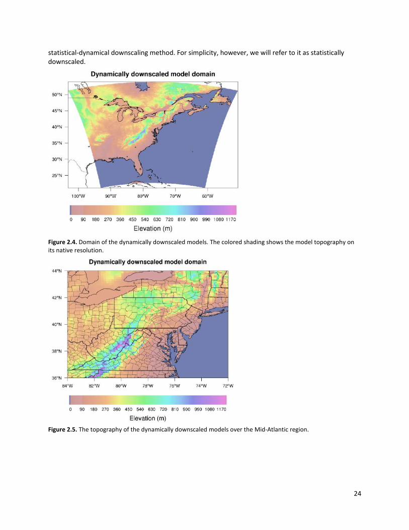
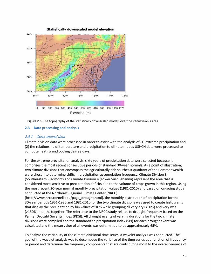
models for forecasting the weather and hydrology. Many simulations are available for each model, including simulations of past conditions with historical concentrations of greenhouse gases and simulations of future conditions with varying concentrations. In this report, we use the simulations with historical greenhouse gases to evaluate the models’ ability to simulate our present climate, and we use simulations using the RCP8.5 greenhouse gas concentration scenario to make projections of future climate. The field of high-resolution regional climate modeling has also evolved since our last report and update. Although the CMIP5 models are state-of-the-art GCMs, the computational expense of running for long timespans at a global scale places limits on the spatial and temporal resolution of the models. A set of methods known as downscaling is used to produce higher-resolution simulations of climate, typically over smaller regions. Downscaling comes in two flavors: dynamical and statistical. There are advantages and disadvantages to each method. For this report, we analyzed data from both dynamically and statistically downscaled climate models. The process of dynamically downscaling a GCM involves running a separate, higher-resolution model within the GCM. Since the domain of the high-resolution model is confined to a smaller region, it is known as a regional climate model, or RCM. The RCM receives information at its boundaries from the GCM and proceeds to simulate climate inside its region using its own resolution and model physics. The dynamically downscaled model data in this report were acquired from the United States Geological Survey (Hostetler et al., 2011), which used two GCMs from CMIP3 (GFDL CM 2.0 and MPI ECHAM5) and one additional GCM (GENMOM). These three models provide conditions at the boundary of the RegCM3 regional climate model, which then simulates the climate over Eastern North America using a high spatial resolution (15 km) and detailed model physics. All of these simulations were run under the SRES A2 emissions scenario. The RCM boundary and topography is shown in Figure 2.4 and a zoomed-in view of the topography over the Mid-Atlantic region is shown in Figure 2.5, which reveals that the main topographic features in Pennsylvania are captured on the RCM grid. Statistical downscaling is an alternative method for obtaining climate simulations at a spatial resolution that is not currently possible in GCMs. Statistical downscaling generally works by developing statistical relationships between coarse-resolution observations that GCMs typically simulate well (such as upper-air pressure) and fine-resolution observations of interest that GCMs do not simulate as well (such as surface precipitation). After the statistical relationships are determined, they are applied to the GCM data to obtain high-resolution climate simulations. One of the advantages of statistical downscaling is that it is rooted in observations. On the other hand, statistical downscaling assumes that the relationship between the coarse and fine scales does not change with time. An additional disadvantage of statistical downscaling is that it is only possible for variables that have an extensive and reliable observational record to develop the statistical relationships with. For example, statistically downscaling conditions in the upper atmosphere is difficult because there are very limited historical observations in this region. For statistically downscaled models, we used the “Downscaled CMIP3 and CMIP5 Climate and Hydrology Projections" archive at http://gdo-dcp.ucllnl.org/downscaled_cmip_projections/ (Brekke et al., 2013), which converts CMIP5 model precipitation, temperature, and other atmospheric variables to a 1/8th-degree domain (about 12-km resolution); see Figure 2.6. In addition, this high-resolution product is used to run a hydrological model (the Variable Infiltration Capacity model) to simulate hydrological conditions such as soil moisture and runoff. In this way, this dataset represents a kind of hybrid

24

statistical-dynamical downscaling method. For simplicity, however, we will refer to it as statistically downscaled.

Figure 2.4. Domain of the dynamically downscaled models. The colored shading shows the model topography on its native resolution.

Figure 2.5. The topography of the dynamically downscaled models over the Mid-Atlantic region.

25

2.3 Data processing and analysis

2.3.1 Observational data Climate division data were processed in order to assist with the analysis of (1) extreme precipitation and (2) the relationship of temperature and precipitation to climate modes USHCN data were processed to compute heating and cooling degree days. For the extreme precipitation analysis, sixty years of precipitation data were selected because it comprises the most recent consecutive periods of standard 30-year normals. As a point of illustration, two climate divisions that encompass the agriculturally rich southeast quadrant of the Commonwealth were chosen to determine shifts in precipitation accumulation frequency. Climate Division 3 (Southeastern Piedmont) and Climate Division 4 (Lower Susquehanna) represent the area that is considered most sensitive to precipitation deficits due to the volume of crops grown in this region. Using the most recent 30-year normal monthly precipitation values (1981-2010) and based on on-going study conducted at the Northeast Regional Climate Center (NRCC) [http://www.nrcc.cornell.edu/page_drought.html], the monthly distribution of precipitation for the 30-year periods 1951-1980 and 1981-2010 for the two climate divisions was used to create histograms that display the precipitation by bin values of 10% while grouping all very dry (<50%) and very wet (>150%) months together. The reference to the NRCC study relates to drought frequency based on the Palmer Drought Severity Index (PDSI). All drought events of varying durations for the two climate divisions were compiled and the standardized precipitation index (SPI) for each drought event was calculated and the mean value of all events was determined to be approximately 65%. To analyze the variability of the climate divisional time series, a wavelet analysis was conducted. The goal of the wavelet analysis was to decompose the variance of the time series as a function of frequency or period and determine the frequency components that are contributing most to the overall variance of

Figure 2.6. The topography of the statistically downscaled models over the Pennsylvania area.

26

the time series. For example, a wavelet analysis of an index of the El Niño phenomenon would show that the dominant frequency component corresponds to a period of several years because El Niño events occur, on average, every few years. The frequency components with enhanced variance (or global wavelet power) are the frequencies at which interesting features may be present, possibly related to some physical mechanism. To detect features embedded in a time series, a wavelet function was used to smooth the time series at different degrees of smoothing to detect features that are most pronounced at a particular frequency. For a brief technical discussion of wavelet analysis the reader is referred to Appendix A. To ensure that results were not generated from random noise, statistical significance of the global power was tested against a red-noise background spectrum, a global wavelet spectrum that favors high global power at low frequencies (Appendix A). Another advantage of wavelet analysis is that two time series, such as precipitation and temperature, can be correlated at a particular frequency. Such a decomposition is referred to as wavelet coherence, which can be regarded as a localized correlation coefficient in both time and frequency. A wavelet coherence analysis was chosen because climate modes are energetic at various frequencies, so that correlation coefficients between climate data and climate indices may be preferentially expressed at particular frequencies. A more simple measure of coherence is global wavelet coherence, a time-averaged version of wavelet coherence. Global coherence, unlike the traditional correlation coefficient, is bounded by zero and one, with zero representing the weakest possible relationship and one representing the strongest possible relationship. Like global wavelet power, the statistical significance of global coherence needed to be assessed. A more technical discussion of wavelet coherence is provided in Appendix A. Before the wavelet analysis was conducted, the monthly climate divisional data were converted to anomalies by removing the 1900-2013 mean annual cycle. The procedure was also conducted on the climate index data. When comparing two time series, the data were first standardized by dividing the anomalies for each month by the standard deviation of the original data for each month. USHCN data were used to compute annual heating and cooling degree days in Pennsylvania since 1900. The number of heating degree days in a given year is computed by summing each day’s deficit of temperature below 65 °F. For example, a day with a mean temperature of 60 °F has 5 degree days. Days above 65 °F are counted as zero. Cooling degree days are computed in an analogous way—by summing each day’s excess above 65 °F.

2.3.2 Climate model data Data from each of the model datasets were extracted for a historical period of 1971-2000 and a future period of 2041-2070. There are several cases where models are missing a few years from the start or end of these time periods. For these cases, we simply used whatever data were available during the time periods. The CMIP5 and statistically downscaled datasets include multiple realizations for some models. For a model with multiple realizations, each realization may start with different initial conditions or have slightly different model physics settings. In this way, the multiple realizations provide some estimate of the uncertainty associated with the model output as a result of random weather variability or uncertainty in the model physics. To reduce each model to a single simulation, we averaged the model’s multiple realizations after extracting the variable of interest. The list of models used is provided in Appendix B.

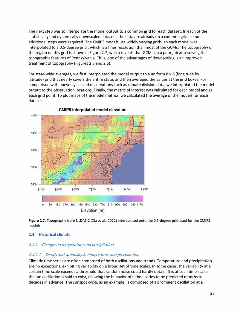
27

The next step was to interpolate the model output to a common grid for each dataset. In each of the statistically and dynamically downscaled datasets, the data are already on a common grid, so no additional steps were required. The CMIP5 models use widely varying grids, so each model was interpolated to a 0.5-degree grid , which is a finer resolution than most of the GCMs. The topography of the region on this grid is shown in Figure 2.7, which reveals that GCMs do a poor job at resolving the topographic features of Pennsylvania. Thus, one of the advantages of downscaling is an improved treatment of topography (Figures 2.5 and 2.6). For state-wide averages, we first interpolated the model output to a uniform 8 × 6 (longitude by latitude) grid that nearly covers the entire state, and then averaged the values at the grid boxes. For comparison with unevenly spaced observations such as climate division data, we interpolated the model output to the observation locations. Finally, the metric of interest was calculated for each model and at each grid point. To plot maps of the model metrics, we calculated the average of the models for each dataset.

Figure 2.7. Topography from NLDAS-2 (Xia et al., 2012) interpolated onto the 0.5-degree grid used for the CMIP5 models.

2.4 Historical climate

2.4.1 Changes in temperature and precipitation

2.4.1.1 Trends and variability in temperature and precipitation Climatic time series are often composed of both oscillations and trends. Temperature and precipitation are no exceptions, exhibiting variability on a broad set of time scales. In some cases, the variability at a certain time scale exceeds a threshold that random noise could hardly obtain. It is at such time scales that an oscillation is said to exist, allowing the behavior of a time series to be predicted months to decades in advance. The sunspot cycle, as an example, is composed of a prominent oscillation at a

28

period of 11 years, which allows scientists to determine the general future behavior of the sunspot cycle. The climate divisional temperature and precipitation considered in this report also exhibited time scales of enhanced variability. Shown in Figure 2.8 are precipitation time series for each climate division. Climate Divisions 1-5 and 6-10 are shown on separate panels for clarity. To highlight temporal variability, the time series have been standardized, which means that the average has been removed and the result has been divided by the standard deviation. To focus attention on variability at longer time scales, the standardized time series have been smoothed using a two-year running average. The most notable features are the wet periods in the early 1960s and the 1970s. Situated between the two wet periods was a dry period called the 1950s drought, which was one of the most prominent droughts in Pennsylvania for the instrumental record. Precipitation variability is very similar throughout the Commonwealth, though the precipitation declines in Climate Divisions 6-10 associated with 1960s were less pronounced compared to those of Climate Divisions 1-5, suggesting spatial differences of drought impacts in Pennsylvania.

Figure 2.8. (a) Standardized anomalies of mean monthly precipitation for Climate Divisions 1-5 for the period 1900-2013. (b) Same as (a) but for climate divisions 6-10. Data have been smoothed by a 2-year running mean. To determine if the large fluctuations in precipitation during the 1960s and 1970s were simply stochastic, unpredictable fluctuations, a global wavelet analysis was conducted together with statistical significance testing (Appendix A). The results from the global power analysis detected significant global wavelet power of precipitation at a period of 27 years for all Climate Divisions except for climate divisions 7-10, the westward-most climate divisions. Indeed, inspection of Figure 2.8 indicates that precipitation in Climate Divisions 5-10 had smaller standardized anomalies during the 1960s and also during the previous and subsequent wet periods. The results suggest that drought conditions are not

29

spatially uniform and thus when examining precipitation, whether past or future changes, spatial inhomogeneity should be considered. The temperature time series are shown in Figure 2.9 and reveal that the climate divisions are highly correlated with each other. High temperatures occurred in the early 1920s, 1930s, 1990s, and 2000s; low temperatures occurred around 1905 and in the late 1920s and 1930s. A period of below-normal temperatures also occurred from 1960 to 1970, which was also a time of below-average precipitation. After a local minimum in mean temperature around 1978, the mean temperature generally increased.

Figure 2.9 (a) Standardized anomalies of mean monthly temperature for Climate Divisions 1-5 for the period 1900-2013. (b) Same as (a) but for Climate Divisions 6-10. A similar global wavelet power analysis was conducted but with mean monthly temperature anomalies for each of the 10 climate divisions. Unlike precipitation, no 27-year periodicity was detected for any of the climate divisions; on the other hand, a statistically significant 2-year periodicity was found for Climate Divisions 1-8, with the global power for Climate Divisions 5-6 being statistically significant at the 99% level. No spatial variability was detected across Pennsylvania.

2.4.1.2 Trends in heating and cooling degree days The annual totals of heating and cooling degree days have also varied widely during the last century (Figure 2.10). Overall, the average annual total of heating degree days during 1981-2010 was 6073, while the average annual total of cooling degree days was only 639. This indicates that mean temperatures in Pennsylvania are more frequently below 65 °F than above, and that the state’s demand for heating is much higher than its demand for cooling. The degree days vary significantly from year to year, however, and there is only modest correlation between the total heating and cooling degree days in a year. Since 1900, neither metric shows a statistically significant trend. However, moderate decreases in heating degree days and increases in cooling degree days are present since 1970. Finally, it

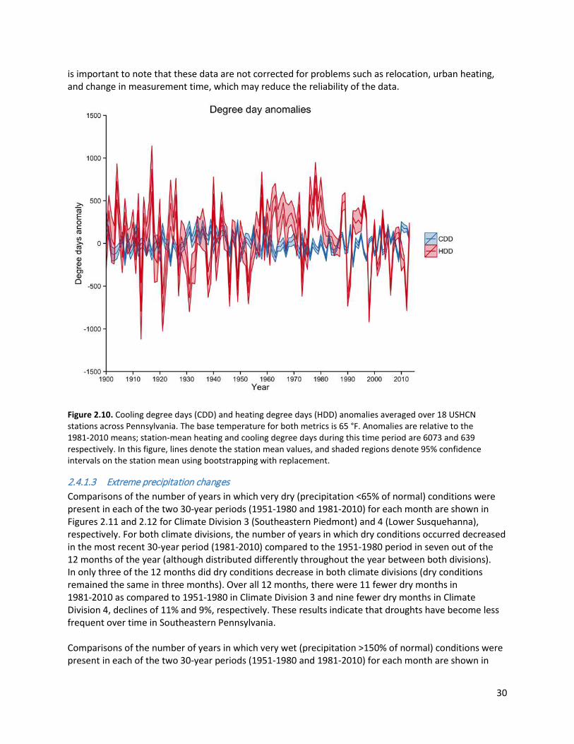
30

is important to note that these data are not corrected for problems such as relocation, urban heating, and change in measurement time, which may reduce the reliability of the data.

Figure 2.10. Cooling degree days (CDD) and heating degree days (HDD) anomalies averaged over 18 USHCN stations across Pennsylvania. The base temperature for both metrics is 65 °F. Anomalies are relative to the 1981-2010 means; station-mean heating and cooling degree days during this time period are 6073 and 639 respectively. In this figure, lines denote the station mean values, and shaded regions denote 95% confidence intervals on the station mean using bootstrapping with replacement.

2.4.1.3 Extreme precipitation changes Comparisons of the number of years in which very dry (precipitation <65% of normal) conditions were present in each of the two 30-year periods (1951-1980 and 1981-2010) for each month are shown in Figures 2.11 and 2.12 for Climate Division 3 (Southeastern Piedmont) and 4 (Lower Susquehanna), respectively. For both climate divisions, the number of years in which dry conditions occurred decreased in the most recent 30-year period (1981-2010) compared to the 1951-1980 period in seven out of the 12 months of the year (although distributed differently throughout the year between both divisions). In only three of the 12 months did dry conditions decrease in both climate divisions (dry conditions remained the same in three months). Over all 12 months, there were 11 fewer dry months in 1981-2010 as compared to 1951-1980 in Climate Division 3 and nine fewer dry months in Climate Division 4, declines of 11% and 9%, respectively. These results indicate that droughts have become less frequent over time in Southeastern Pennsylvania. Comparisons of the number of years in which very wet (precipitation >150% of normal) conditions were present in each of the two 30-year periods (1951-1980 and 1981-2010) for each month are shown in

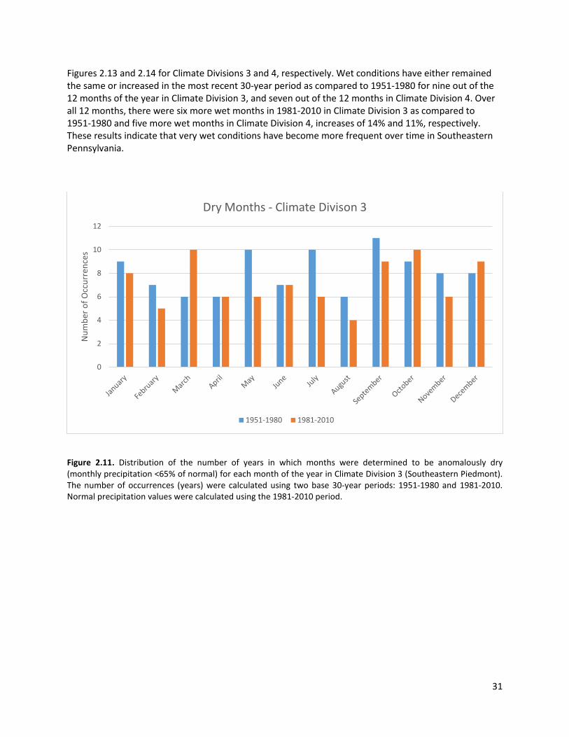
31

Figures 2.13 and 2.14 for Climate Divisions 3 and 4, respectively. Wet conditions have either remained the same or increased in the most recent 30-year period as compared to 1951-1980 for nine out of the 12 months of the year in Climate Division 3, and seven out of the 12 months in Climate Division 4. Over all 12 months, there were six more wet months in 1981-2010 in Climate Division 3 as compared to 1951-1980 and five more wet months in Climate Division 4, increases of 14% and 11%, respectively. These results indicate that very wet conditions have become more frequent over time in Southeastern Pennsylvania.

Figure 2.11. Distribution of the number of years in which months were determined to be anomalously dry (monthly precipitation <65% of normal) for each month of the year in Climate Division 3 (Southeastern Piedmont). The number of occurrences (years) were calculated using two base 30-year periods: 1951-1980 and 1981-2010. Normal precipitation values were calculated using the 1981-2010 period.

0

2

4

6

8

10

12

Num

ber o

f Occ

urre

nces

Dry Months - Climate Divison 3

1951-1980 1981-2010

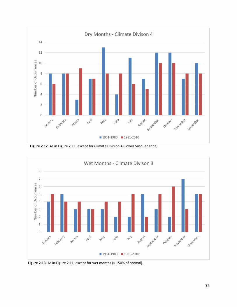
32

Figure 2.12. As in Figure 2.11, except for Climate Division 4 (Lower Susquehanna).

Figure 2.13. As in Figure 2.11, except for wet months (> 150% of normal).

0

2

4

6

8

10

12

14

Num

ber o

f Occ

urre

nces

Dry Months - Climate Divison 4

1951-1980 1981-2010

0

1

2

3

4

5

6

7

8

Num

ber o

f Occ

urre

nces

Wet Months - Climate Divison 3

1951-1980 1981-2010

33

Figure 2.14. As in Figure 2.13, except for Climate Division 4 (Lower Susquehanna).

As a result of the combined effects of fewer drought occurrences as well as an increase in very wet months across the southeastern portion of Pennsylvania, these findings support the fact that Southeastern Pennsylvania has become more “drought resistant” over the course of the last few decades. In other words, water resources have been more abundant over recent years as compared to previous decades. The distribution of precipitation in 10% increments between 50% and 150% as well as <50% and >150% is shown for 1951-1980 using 1981-2010 as the normal period in Figure 2.15 for Climate Divisions 3 and 4. Note the greater frequency of events less than 100% indicating this period was notably drier than the most recent 30 years. Specifically, the count of >50 (out of a possible 360) months with less than 50% of normal precipitation reflects the droughts that occurred in the 1950s and 1960s in this region. Figure 2.16 shows the precipitation distribution for 1981-2010. Note the magnitude of the bar representing >150% of normal precipitation, indicating a substantial rise in extreme precipitation events during this period.

0

1

2

3

4

5

6

7

8

Num

ber o

f Occ

urre

nces

Wet Months - Climate Divison 4

1951-1980 1981-2010

34

Figure 2.15. The frequency distribution of monthly precipitation amounts for the Southeastern Piedmont (top) and the Lower Susquehanna (bottom) for 1951-1980 based on the 1981-2010 normals.

35

Figure 2.16. Same as Figure 2.15 except for 1981-2010.

2.4.2 Potential causes of changes

2.4.2.1 Climate modes Climate modes are recurring spatial patterns in sea surface temperature (SST), sea-level pressure (SLP), and other climate variables that operate on an array of time scales, ranging from monthly to multidecadal. Perhaps the most well-known climate modes are the North Atlantic Oscillation (NAO) and the El Niño-Southern Oscillation (ENSO), with the latter having regional- to global-scale impacts. Other climate modes include the Atlantic Multidecadal Oscillation (AMO), Pacific Decadal Oscillation (PDO), and Pacific-North American teleconnection pattern (PNA). A discussion of each climate mode is provided

36

below together with descriptions of the physical mechanisms governing each climate mode. A brief survey of climate-mode impacts on Northeast climate variability is also provided. The NAO characterizes the seesaw pattern of SLP over the North Atlantic consisting of the Icelandic Low and the Azores High. To better monitor the evolution of the NAO, an NAO index has been constructed, which is defined as the normalized SLP difference between the Azores High and the Icelandic Low (Hurrell et al., 2003). This index offers a simple interpretation: when the NAO index is negative the pressure difference between the two centers of action is weaker than normal; when the NAO index is positive the pressure difference is stronger than normal. The NAO index has allowed the quantification of various statistical and frequency-domain properties of the NAO. More specifically, the NAO was found to have enhanced variance at the decadal timescale, though the physical mechanisms governing this characteristic time scale are uncertain (Hurrell et al., 2003). The NAO index has also been found to be correlated with both precipitation and temperature across the Northeast United States, particularly in the winter when the atmosphere is most dynamically active (Serreze et al., 1998; Seager et al., 2010). ENSO is a 2-7 year oscillation in equatorial Pacific SST consisting of two phases: (1) the El-Niño phase, characterized by positive SST anomalies, weaker than normal trade winds, and enhanced atmospheric convection (vertical motion) over the equator; and (2) the La-Niña phase, characterized by below-normal SSTs in the equatorial Pacific together with reduced convection and stronger-than-normal trade winds. A common metric for measuring the strength and evolution of ENSO is the Southern Oscillation Index (SOI), defined as the SLP difference between Darwin, Australia and Tahiti (Trenberth, 1984). The index measures the strength of the trade winds. The changes in tropical convection associated with each phase of ENSO alters the mid-latitude large-scale circulation pattern in the Northern-Hemisphere boreal winter (Bjerknes, 1969; Horel and Wallace, 1981), with an El-Niño phase bringing more snowfall to the East Coast of the United States, including eastern Pennsylvania (Patten et al., 2003; Seager et al., 2010). Snowfall is particularly enhanced during El-Niño phases when the NAO is a negative, suggesting covariability. The increased snowfall may be the result of increased East Coast storm frequency during El-Niño events (Eichler and Higgins, 2006). The AMO describes changes in mean SSTs across the North Atlantic Ocean. Unlike ENSO and the NAO, the AMO exhibits enhanced variance at periods of 20-80 years (Enfield et al., 2001). To measure the strength and evolution of the AMO, an index has been constructed that is defined as the detrended average SST in the North Atlantic basin from 0° to 70°N (Enfield et al., 2001). Variations in the AMO index are associated with changes in the overlying atmosphere and long-time scale oceanic processes such as the thermohaline circulation. The AMO has been shown to impact drought frequency across the United States, though only weakly in the Northeast United States (McCabe et al., 2004). The PDO is another multidecadal mode of variability in the climate system with characteristic time scales of 20 to 70 years (Mantua et al., 1997; Mantua and Hare, 2002). The PDO index is defined as the leading empirical orthogonal function (EOF) of SSTs across the North Pacific Ocean. The PDO index captures most of the spatial variability of SSTs in the North Pacific, with a negative phase consisting of negative SST anomalies along the west coast of the United States and positive anomalies in the central North Pacific (Mantua et al., 1997; Mantua and Hare, 2002). The spatial pattern associated with the positive phase is opposite to that of the negative phase, consisting of positive SST anomalies along the west coast of the United States and negative anomalies in the central North Pacific Ocean. The PDO has been related to drought across North America and streamflow variability across the Northeast United States (McCabe et al., 2004; Labat, 2010). The PDO may not, however, directly influence North American

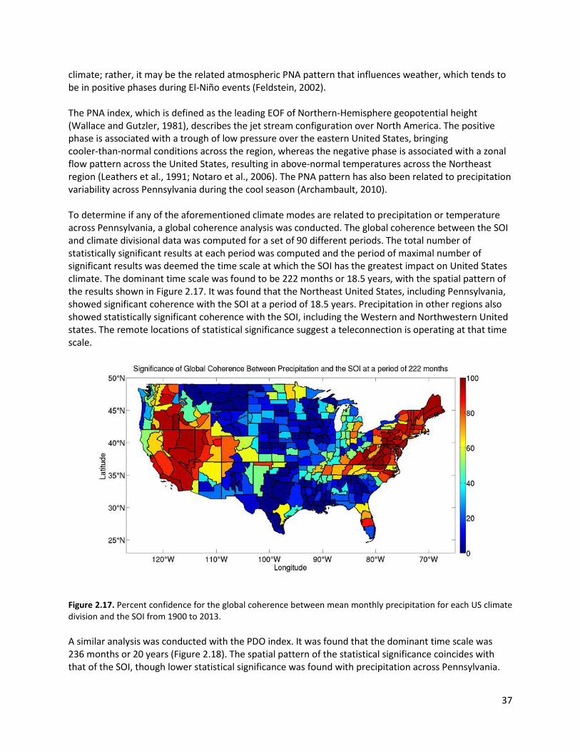
37

climate; rather, it may be the related atmospheric PNA pattern that influences weather, which tends to be in positive phases during El-Niño events (Feldstein, 2002). The PNA index, which is defined as the leading EOF of Northern-Hemisphere geopotential height (Wallace and Gutzler, 1981), describes the jet stream configuration over North America. The positive phase is associated with a trough of low pressure over the eastern United States, bringing cooler-than-normal conditions across the region, whereas the negative phase is associated with a zonal flow pattern across the United States, resulting in above-normal temperatures across the Northeast region (Leathers et al., 1991; Notaro et al., 2006). The PNA pattern has also been related to precipitation variability across Pennsylvania during the cool season (Archambault, 2010). To determine if any of the aforementioned climate modes are related to precipitation or temperature across Pennsylvania, a global coherence analysis was conducted. The global coherence between the SOI and climate divisional data was computed for a set of 90 different periods. The total number of statistically significant results at each period was computed and the period of maximal number of significant results was deemed the time scale at which the SOI has the greatest impact on United States climate. The dominant time scale was found to be 222 months or 18.5 years, with the spatial pattern of the results shown in Figure 2.17. It was found that the Northeast United States, including Pennsylvania, showed significant coherence with the SOI at a period of 18.5 years. Precipitation in other regions also showed statistically significant coherence with the SOI, including the Western and Northwestern United states. The remote locations of statistical significance suggest a teleconnection is operating at that time scale.

Figure 2.17. Percent confidence for the global coherence between mean monthly precipitation for each US climate division and the SOI from 1900 to 2013. A similar analysis was conducted with the PDO index. It was found that the dominant time scale was 236 months or 20 years (Figure 2.18). The spatial pattern of the statistical significance coincides with that of the SOI, though lower statistical significance was found with precipitation across Pennsylvania.

38

Figure 2.18. Percent confidence for the global coherence between mean monthly precipitation for each US climate division and the PDO index from 1900 to 2013. The statistical significance also appears to be most pronounced across eastern Pennsylvania, highlighting the spatial variability in the teleconnection. It is important to note that the PDO and SOI are related on all time scales (Newmann, 2003), which explains the similarity in the SOI-precipitation and PDO-precipitation relationships. A global coherence analysis determined that temperature, unlike precipitation across Pennsylvania, is not coherent with the PDO index or the SOI at the 22-year time scale. The PDO index, however, was found to be coherent with temperature at period of 8 months. The spatial pattern identified at this time scale consisted of a single large region of statistically significant coherence encompassing over 90% of the 344 United States climate divisions, including all 10 of the Pennsylvania climate divisions. The connection between Pennsylvania precipitation and the SOI indicates that ENSO may have played a role in the 1960s drought and possibly the subsequent wet period. ENSO associations with precipitation may therefore mitigate or enhance the effects of global warming on regional climate depending on the regime of ENSO. Such associations may also be problematic when making projections about future Pennsylvania climate, given that climate model projections of the future state of ENSO are inconsistent. Uncertainties in the future state of ENSO could manifest as uncertainties in future changes of precipitation across Pennsylvania.

2.4.2.2 Atmospheric composition The composition of the Earth’s atmosphere, including greenhouse gases that contribute to warming and aerosols that contribute to cooling, changed significantly during the last century. For example, the concentration of CO2 in the atmosphere was less than 300 parts per million (ppm) in 1900 and is currently just below 400 ppm. To examine the impact of these atmospheric changes on Pennsylvania’s climate, we compare simulations from CMIP5 GCMs using two different sets of radiative forcings. The first set uses “historical” forcings, which represent the best approximation of the actual evolution of

39

radiative forcing over the last century, including changes in greenhouse gases, aerosols, solar output, and volcanic eruptions. The second set uses “natural” only changes in the forcing. That is, the only changes in radiative forcing are due to changes in volcanic eruptions and changes in solar output. Radiative forcings that could change as a result of human influence, such the concentrations of CO2 and tropospheric sulfate aerosols, are fixed at constant or seasonally varying values (usually pre-industrial) in the second set. Both sets of models may exhibit a small temperature trend over time as a result of the model adjusting to equilibrium. We did not correct for this drift, although since it is present in both sets the impact on the analysis should be negligible. If the models are capable of correctly simulating the response of temperature to radiative forcing, the time series of temperature from the set of historical models (which include all radiative forcings, including anthropogenic forcing) should closely match the temperatures that were actually observed. Then any difference between the historically forced models and the naturally forced models would indicate a modeled anthropogenic influence. The historically forced models do capture the main long-term trends in Pennsylvania climate, which were described in our 2012 update: a long-term warming trend interrupted by a brief mid-century cooling (Figure 2.19). In particular the warming trend since the 1960s is well-captured by the historically forced models but is not present in the naturally forced models, and by 1990 the 95% confidence intervals of the two sets of models no longer overlap, which suggests that the warming is a result of anthropogenic influence. By the early 2000s, the models that include historic anthropogenic forcing are approximately 1 °C (1.8 °F) warmer than the models with natural forcing only; thus, in these model simulations, anthropogenic climate change has already warmed Pennsylvania by about 1 °C (1.8 °F).

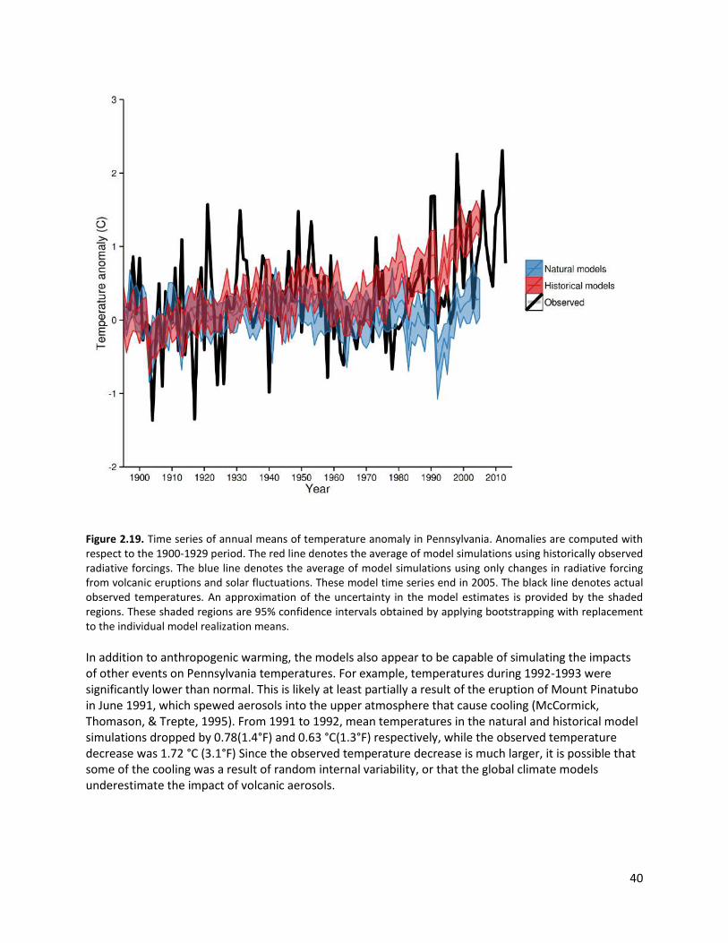
40

Figure 2.19. Time series of annual means of temperature anomaly in Pennsylvania. Anomalies are computed with respect to the 1900-1929 period. The red line denotes the average of model simulations using historically observed radiative forcings. The blue line denotes the average of model simulations using only changes in radiative forcing from volcanic eruptions and solar fluctuations. These model time series end in 2005. The black line denotes actual observed temperatures. An approximation of the uncertainty in the model estimates is provided by the shaded regions. These shaded regions are 95% confidence intervals obtained by applying bootstrapping with replacement to the individual model realization means. In addition to anthropogenic warming, the models also appear to be capable of simulating the impacts of other events on Pennsylvania temperatures. For example, temperatures during 1992-1993 were significantly lower than normal. This is likely at least partially a result of the eruption of Mount Pinatubo in June 1991, which spewed aerosols into the upper atmosphere that cause cooling (McCormick, Thomason, & Trepte, 1995). From 1991 to 1992, mean temperatures in the natural and historical model simulations dropped by 0.78(1.4°F) and 0.63 °C(1.3°F) respectively, while the observed temperature decrease was 1.72 °C (3.1°F) Since the observed temperature decrease is much larger, it is possible that some of the cooling was a result of random internal variability, or that the global climate models underestimate the impact of volcanic aerosols.

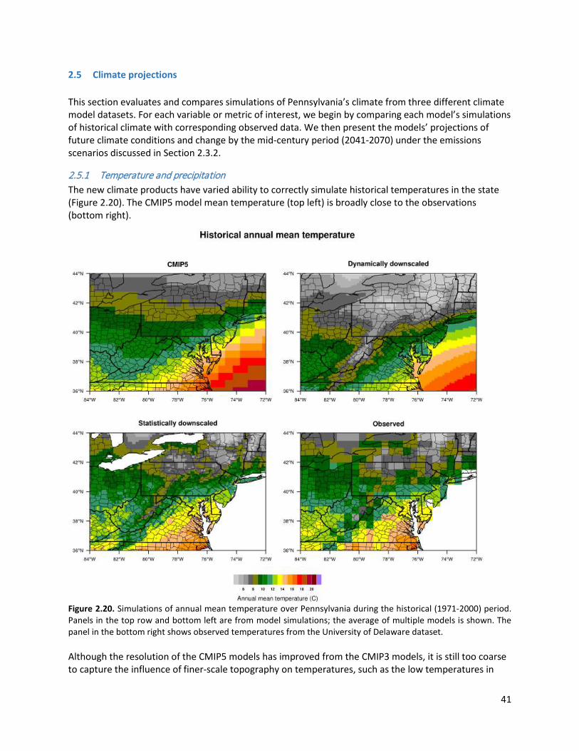
41

2.5 Climate projections This section evaluates and compares simulations of Pennsylvania’s climate from three different climate model datasets. For each variable or metric of interest, we begin by comparing each model’s simulations of historical climate with corresponding observed data. We then present the models’ projections of future climate conditions and change by the mid-century period (2041-2070) under the emissions scenarios discussed in Section 2.3.2.

2.5.1 Temperature and precipitation The new climate products have varied ability to correctly simulate historical temperatures in the state (Figure 2.20). The CMIP5 model mean temperature (top left) is broadly close to the observations (bottom right).

Figure 2.20. Simulations of annual mean temperature over Pennsylvania during the historical (1971-2000) period. Panels in the top row and bottom left are from model simulations; the average of multiple models is shown. The panel in the bottom right shows observed temperatures from the University of Delaware dataset. Although the resolution of the CMIP5 models has improved from the CMIP3 models, it is still too coarse to capture the influence of finer-scale topography on temperatures, such as the low temperatures in

42

Potter and Tioga counties and following the Appalachian Mountains through the southern part of the state and into West Virginia. The dynamically downscaled model products have sufficient resolution to correctly capture this spatial temperature pattern. However, these models underestimate temperature by several degrees. These models are primarily based on the older CMIP3 dataset, and we found a similar consistent cold bias in the previous assessment (Shortle et al., 2009). Finally, the statistically downscaled CMIP5 model mean temperature is essentially identical to the observed annual mean temperature, which is expected because these statistical model products have been bias-corrected. By mid-century, all three model products indicate that the entire state and surrounding regions will have warmed significantly (Figure 2.21).

In both the CMIP5 and statistically downscaled CMIP5 datasets, mid-century temperatures in the Philadelphia region are projected to be similar to historical temperatures in the Richmond, VA area. Similarly, Pittsburgh’s temperatures are projected to resemble the historically observed temperatures in

Figure 2.21. Projections of annual mean temperature in the Pennsylvania region during the mid-century period (2041-2070).

43

the Baltimore-Washington area. The mean warming across the state simulated by these models is generally 3.0-3.5 °C (5.4-6.3°F) (Figure 2.22). The CMIP5 model mean change is 3.0-3.3 °C (5.4-6.0 °F) across nearly the entire state. The statistically downscaled CMIP5 model mean change is 3.3-3.5 °C (5.9-6.3°F ) in the northern half of the state and 3.0-3.3 °C (5.4-6.0°F) in the southern half. Finally, the dynamically downscaled dataset model mean change is only 1.5-1.8 °C (2.7-3.2°F) across the western half of the state and 1.8-2.1 °C (3.2-3.8 °F ) across the eastern half. The reduced warming is likely at least partially because these models rely on the A2 emissions scenario, in which the buildup of greenhouse gases in the atmosphere occurs at a slower rate than in the RCP8.5 scenario that the CMIP5 models use. Globally, the RCP8.5 scenario has about 30-40% more warming than the A2 scenario by mid-century. At most, this accounts for about half the difference observed between dynamically downscaled results and the CMIP5 results, suggesting substantial differences in the models themselves.

Figure 2.22. Projections of change in annual mean temperature in the Pennsylvania region by the mid-century period (2041-2070) relative to the historical period (1971-2000). The panels on the left are based on the RCP8.5 emissions scenario, and the panel on the right is based on the A2 scenario.

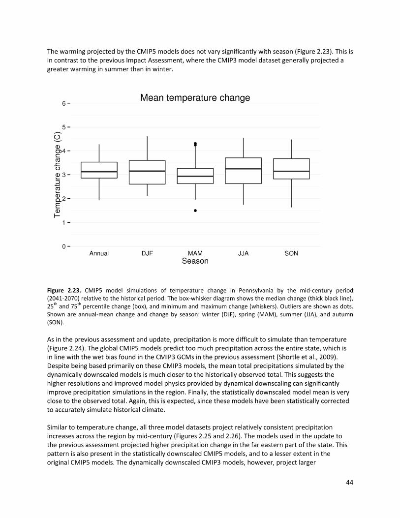
44

The warming projected by the CMIP5 models does not vary significantly with season (Figure 2.23). This is in contrast to the previous Impact Assessment, where the CMIP3 model dataset generally projected a greater warming in summer than in winter.

Figure 2.23. CMIP5 model simulations of temperature change in Pennsylvania by the mid-century period (2041-2070) relative to the historical period. The box-whisker diagram shows the median change (thick black line), 25th and 75th percentile change (box), and minimum and maximum change (whiskers). Outliers are shown as dots. Shown are annual-mean change and change by season: winter (DJF), spring (MAM), summer (JJA), and autumn (SON). As in the previous assessment and update, precipitation is more difficult to simulate than temperature (Figure 2.24). The global CMIP5 models predict too much precipitation across the entire state, which is in line with the wet bias found in the CMIP3 GCMs in the previous assessment (Shortle et al., 2009). Despite being based primarily on these CMIP3 models, the mean total precipitations simulated by the dynamically downscaled models is much closer to the historically observed total. This suggests the higher resolutions and improved model physics provided by dynamical downscaling can significantly improve precipitation simulations in the region. Finally, the statistically downscaled model mean is very close to the observed total. Again, this is expected, since these models have been statistically corrected to accurately simulate historical climate. Similar to temperature change, all three model datasets project relatively consistent precipitation increases across the region by mid-century (Figures 2.25 and 2.26). The models used in the update to the previous assessment projected higher precipitation change in the far eastern part of the state. This pattern is also present in the statistically downscaled CMIP5 models, and to a lesser extent in the original CMIP5 models. The dynamically downscaled CMIP3 models, however, project larger

45

precipitation increases in the northwestern part of the state. All of these differences are relatively small, however.

Figure 2.24. Simulations of annual total precipitation over Pennsylvania during the historical (1971-2000) period. The panels in the top row and bottom left are from model simulations. The panel in the bottom right shows observed precipitation totals from the University of Delaware dataset.

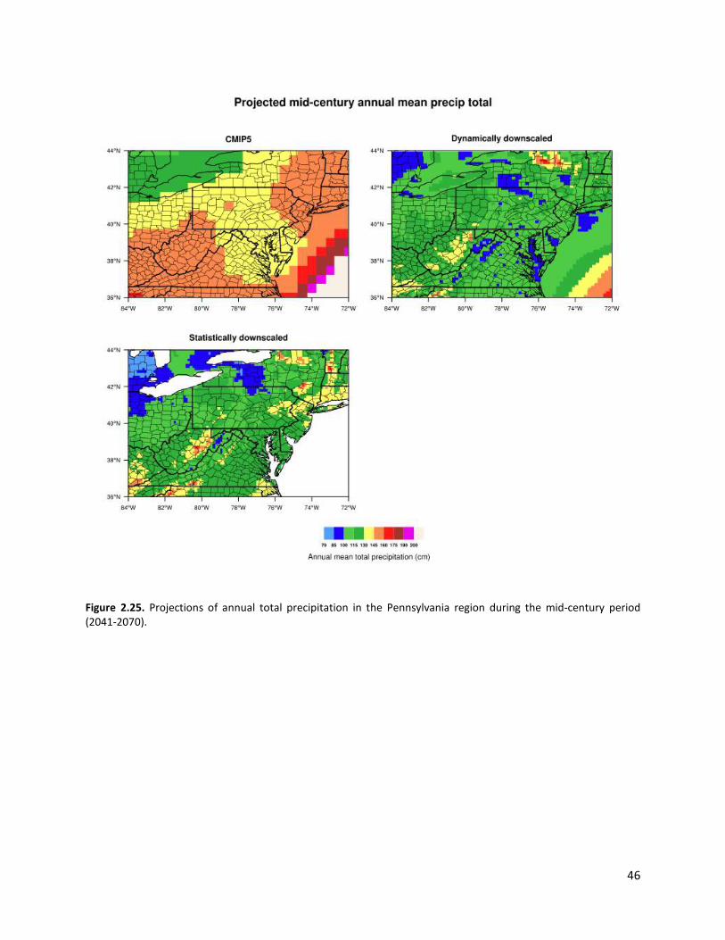
46

Figure 2.25. Projections of annual total precipitation in the Pennsylvania region during the mid-century period (2041-2070).

47

Figure 2.26. Projections of change in annual total precipitation in the Pennsylvania region by the mid-century period (2041-2070) relative to the historical period (1971-2000). The panels on the left are based on the RCP8.5 emissions scenario, and the panel on the right is based on the A2 scenario. In the Mid-Atlantic region, climate models have consistently projected large increases in winter precipitation totals and smaller increases or even decreases in summer and fall precipitation totals. This pattern continues in the latest CMIP5 models (Figure 2.27). However, the median model change four all four seasons is positive, indicating increased precipitation throughout the year.

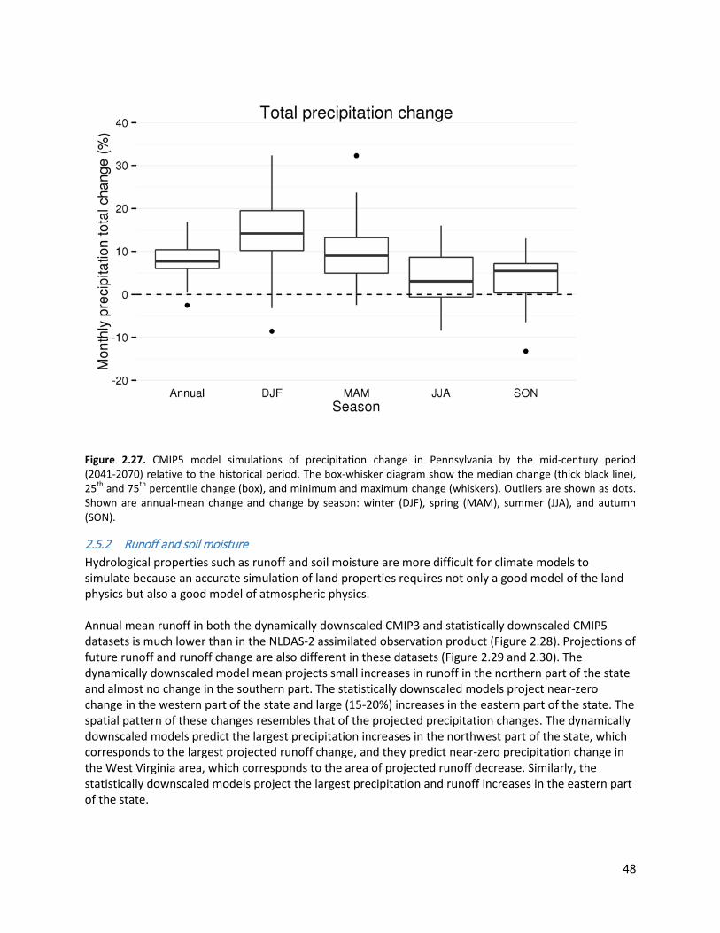
48

Figure 2.27. CMIP5 model simulations of precipitation change in Pennsylvania by the mid-century period (2041-2070) relative to the historical period. The box-whisker diagram show the median change (thick black line), 25th and 75th percentile change (box), and minimum and maximum change (whiskers). Outliers are shown as dots. Shown are annual-mean change and change by season: winter (DJF), spring (MAM), summer (JJA), and autumn (SON).

2.5.2 Runoff and soil moisture Hydrological properties such as runoff and soil moisture are more difficult for climate models to simulate because an accurate simulation of land properties requires not only a good model of the land physics but also a good model of atmospheric physics. Annual mean runoff in both the dynamically downscaled CMIP3 and statistically downscaled CMIP5 datasets is much lower than in the NLDAS-2 assimilated observation product (Figure 2.28). Projections of future runoff and runoff change are also different in these datasets (Figure 2.29 and 2.30). The dynamically downscaled model mean projects small increases in runoff in the northern part of the state and almost no change in the southern part. The statistically downscaled models project near-zero change in the western part of the state and large (15-20%) increases in the eastern part of the state. The spatial pattern of these changes resembles that of the projected precipitation changes. The dynamically downscaled models predict the largest precipitation increases in the northwest part of the state, which corresponds to the largest projected runoff change, and they predict near-zero precipitation change in the West Virginia area, which corresponds to the area of projected runoff decrease. Similarly, the statistically downscaled models project the largest precipitation and runoff increases in the eastern part of the state.

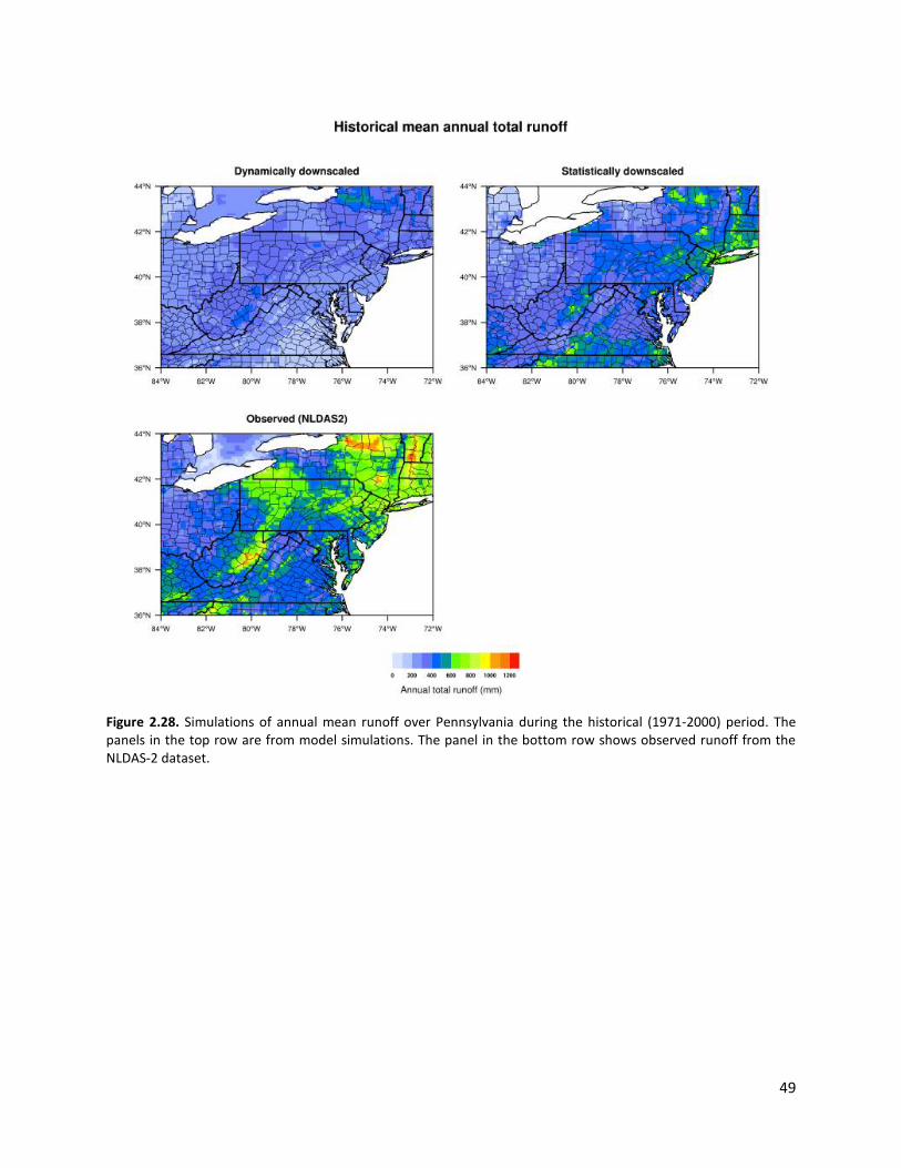
49

Figure 2.28. Simulations of annual mean runoff over Pennsylvania during the historical (1971-2000) period. The panels in the top row are from model simulations. The panel in the bottom row shows observed runoff from the NLDAS-2 dataset.

50

Projected mid-century mean annual total runoff

Figure 2.29. Projections of annual mean runoff in the Pennsylvania region during the mid-century period (2041-2070). The panel on the left is based on the A2 scenario, and the panel on the right is based on the RCP8.5 emissions scenario.

Projected annual mean runoff change

Figure 2.30. Projections of change in annual mean runoff in the Pennsylvania region by the mid-century period (2041-2070) relative to the historical period (1971-2000). The panel on the left is based on the A2 scenario, and the panel on the right is based on the RCP8.5 emissions scenario.

51

Figure 2.31. Simulations of annual mean soil moisture in the Pennsylvania region during the historical (1971-2000) period. Panels in the top row are from model simulations. The panel in the bottom row shows observed soil moisture from the NLDAS-2 product. Simulations of total soil moisture are similarly divergent (Figure 2.31). Soil moisture in the dynamically downscaled models is almost twice that in the NLDAS-2 product, and soil moisture in the statistically downscaled models is almost half that in NLDAS-2. Projections of future soil moisture and soil moisture change (Figures 2.32 and 2.33) are similarly scattered. These projections generally resemble those of runoff and precipitation change; the dynamically downscaled models project increasing soil moisture in the northern part of the state and decreasing soil moisture in many areas along or south of the state border.

52

Projected mid-century annual mean soil moisture

Figure 2.32. Projections of annual mean soil moisture in the Pennsylvania region during the mid-century period (2041-2070). The panel on the left is based on the A2 scenario, and the panel on the right is based on the RCP8.5 emissions scenario.

Model mean annual soil moisture change

Figure 2.33. Projections of change in annual mean soil moisture in the Pennsylvania region by the mid-century period (2041-2070) relative to the historical period (1971-2000). The panel on the left is based on the A2 scenario, and the panel on the right is based on the RCP8.5 emissions scenario.

53

2.5.3 Extreme precipitation While there has been a 10% increase in average annual precipitation across Pennsylvania during the past century, there has been a noteworthy increase in the number of extreme precipitation events in more recent times. According to the National Climate Assessment issued in May, 2014, in the period 1958-2012, there was a 71% increase in the frequency of the heaviest 1% precipitation events in the Northeast United States, including Pennsylvania (Karl et al., 2009). Given the decrease in ‘dry months’ during the last 30 years, it would be wise to discern the expected trends in the ensemble regional climate models for monthly precipitation anomalies, based on the current normal, for the period 2020-2050 in the two climate divisions that were part of this case study, the Southeastern Piedmont and Lower Susquehanna region. To study projected changes in increased precipitation, we extracted precipitation data from the statistically downscaled CMIP5 models for 2020-2050 and interpolated the data to the centers of the Southeastern Piedmont and Lower Susquehanna climate divisions (Divisions 3 and 4). The lower RCP scenario (RCP2.6) was used since this is the most conservative outcome and the projections are for a shorter time scale (the next 30 years). Figures 2.34-2.37 show the projected 2020-2050 wet-and dry-month frequency in Climate Divisions 3 and 4 using the same criteria as in Section 2.4.1.3; the figures are therefore directly comparable to Figures 2.11-2.14, which describe wet-and dry-month frequency for these climate divisions for 1951-1980 and 1981-2010. The most occurrences of drought are anticipated to occur in the autumn (Figures 2.34 and 2.35), which is opposite the historical trend (the most frequent wet months have been in September-October). For wet months in Climate Division 3 (Figure 2.36), the fewest occurrences are also anticipated to occur in the autumn (also opposite the current trend). In Climate Division 4 (Figure 2.37), the fewest occurrences are anticipated to occur in the summer while the most frequent are expected to occur in December and January.

Figure 2.34. The number of dry months (values less than 65% of the 1981-2010 normal) by actual months as projected by the 53-member ensemble of CMIP5 using the RCP2.6 scenario that has been bias-corrected and statistically downscaled for grid boxes that match the center of the Southeast Piedmont climate division.

54

Figure 2.35. Same as Figure 2.34, except for the Lower Susquehanna climate division.

Figure 2.36. The number of wet months (values greater than 150% of the 1981-2010 normal) by actual months as projected by the 53-member ensemble of CMIP5 using the RCP2.6 scenario that has been bias-corrected and statistically downscaled for grid boxes that match the center of the Southeast Piedmont climate division.

55

Figure 2.37. Same as Figure 2.30, except for the Lower Susquehanna climate division. Figure 2.38 shows the precipitation histogram for 2020-2050, which can be directly compared to the histograms for 1951-1980 and 1981-2010 (Figures 2.15 and 2.16). The histogram has been ‘normalized’ for comparison with the previous figures since over 19,000 months are represented in these displays. The most notable feature is the spike in the anticipated occurrence of months with greater than 150% of the current average precipitation in Climate Division 3. Though there is not quite as pronounced of a spike in Climate Division 4, there is still an elevated frequency in the anticipated occurrence of months with greater than 150% of the current average precipitation. To summarize the projections of extreme precipitation, the most advanced climate simulations, which have been bias-corrected and downscaled statistically to account for terrain and other local effects in Pennsylvania, point to a continued rise in very wet months in the period 2020-2050. In fact, while it is possible that the signal showing a shift to wetter periods in the winter and more frequent dry times (months with <65% of average precipitation) in the autumn could be attributed to random variations in the ensemble projections, the trend is notable and certainly a change from the current regime. These results are consistent with a tendency for drought resistance to persist in the agriculturally rich climate divisions of southern and central Pennsylvania.

56

Figure 2.38. The values show the equivalent frequency of monthly precipitation based on the 1981-2010 normal and as projected by the 53-member ensemble of CMIP5 using RCP2.6 that has been bias-corrected and statistically downscaled for grid boxes that match the center of the Southeast Piedmont (top) and Lower Susquehanna (bottom) climate divisions.

2.6 Summary Our third assessment of climate change in Pennsylvania builds on our previous findings and is largely consistent with them. The main findings are:

• Observed long-term changes in Pennsylvania’s temperature are human-induced. Pennsylvania has undergone a long-term warming of more than 1 °C (1.8°F ) over the past 110 years, interrupted by a brief cooling period in the mid-20th century, which is simulated by climate models only when anthropogenic forcing, mainly increases in greenhouse gases, are included.

57

• Climate modes have a significant impact on Pennsylvania’s climate. A literature review indicates that the North Atlantic Oscillation, the El Niño/Southern Oscillation, the Pacific Decadal Oscillation, and the Pacific North American pattern all influence Pennsylvania’s temperature and (especially) precipitation. Our wavelet analysis suggests that climate-mode effects are dominant at periods of about 20 years for precipitation and are consistent with teleconnection patterns throughout the US.

• Heating and cooling degree changes reflect recent warming. Moderate decreases in heating degree days and increases in cooling degree days are present since 1970.

• Changes in above- and below-normal precipitation reflect the general wetting trend. Since 1950, droughts have become less frequent and very wet conditions have become more frequent in Southeastern Pennsylvania (where the analysis was limited to).

• The representation of Pennsylvania’s climate by Global Climate Models has improved. The newer global climate models used in this report (CMIP5) do not have the cold bias of the older models though they are still too wet. The newer dynamically downscaled models retain the cold bias but have improved precipitation simulations.

• Pennsylvania’s current warming and wetting trends will continue at an accelerated rate. Using an emissions scenario that continues the current emissions trend, the RCP8.5 scenario, we project that by the middle of the 21st century, Pennsylvania will be about 3 °C (5.4°F) warmer than it was at the end of the 20th century. The corresponding annual precipitation increase is expected to be 8%, with a winter increase of 14%. The likelihood for drought is expected to decrease while months with above-normal precipitation are expected to increase.

• More research is needed to improve hydrological projections. Runoff and soil moisture simulations show substantial differences from products based on observations. The existing models suggest modest but significant increases in annual-mean runoff and small changes in annual-mean soil moisture.

58

Appendix A In this report we adopt the Morlet wavelet, which is given by

𝜓0(𝜂) = 𝜋−1/4𝑒𝑖𝑖𝑖𝑒−12𝑖

2, (2)

where 𝜓0 is the Morlet wavelet, 𝜔 is the dimensionless frequency, and η is the dimensionless time. The Morlet wavelet with ω = 6 is recommended for identifying features of geophysical time series (Grinsted et al., 2004). The wavelet transform of a time series (𝑥𝑛; n = 1,...,N) is defined as the is defined as

𝑊𝑛𝑋(𝑠) = �𝛿𝛿

𝑠∑ 𝑥𝑛′𝜓0[(𝑛′ − 𝑛)] 𝛿𝛿

𝑠𝑁𝑛′=1 ],

where 𝛿𝛿, is a uniform timestep, s is the scale of the Morlet wavelet, and 𝜂 = 𝑠 ⋅ 𝛿. The wavelet power at a given scale and time is then given by |𝑊𝑛

𝑋(𝑠)| and averaging 𝑊𝑛𝑋(𝑠) over the time index results

in the global wavelet power spectrum. The significance of both global and local wavelet power at a given frequency and time can be tested against a red-noise background. The threshold for wavelet power to be significant depends strongly on the autocorrelation structure of time series. The reader is referred to Torrence and Compo (1998) and Grinsted et al. (2004) for a more detailed discussion of significance testing used in this report.

To find the relationships between two time series, a global coherence analysis was conducted to identify time scales at which precipitation (and temperature) were most strongly related with various climate indices. Global coherence is defined by

𝐺𝐶(𝑠) = �𝑊𝑋𝑋(𝑠)�2

(∫|𝑊𝑋(𝑠,𝛿)|2𝑑𝛿)(∫|𝑊𝑋(𝑠,𝛿)|2𝑑𝛿) ,

where 𝑊𝑋(𝑠, 𝛿) is the wavelet power at time 𝛿 and scale s , and

𝑊𝑋𝑋(𝑠) = �𝑊𝑋 (𝑠, 𝛿)𝑊𝑋∗(𝑠, 𝛿)𝑑𝛿 ,

with the asterisk denoting the complex conjugate (Elsayed, 2006). Equation (5) measures the correlation between two time series in a time interval T and at a scale s. In this report T is set to the length of the time series. Statistical significance of 𝐺𝐶(𝑠) was computed using Monte Carlo methods by generating red-noise time series with the same lengths and autocorrelation coefficients as the two input data series and computing 𝐺𝐶(𝑠) for each pair of red-noise time series. The resulting distribution of 𝐺𝐶(𝑠) at each scale was then used to estimate the significance of the global coherence estimates.

(3)

(5)

(6)

59

Appendix B Table 2.1 CMIP5 global climate models used in this report. CMIP5 model availability varies due to differences in models, modeling groups, and data servers. Columns “Temperature,” “Precipitation,” and “Forced temperature” denote the models used to analyze temperature, precipitation, and historical temperature under different forcing conditions respectively. “Realization” followed by a number indicates that one realization was used (with the used realization number corresponding to the number). “Ensemble” indicates that an average of multiple realizations was used, and “Physics” denotes that an average of model output using multiple physics options was used.

Model Temperature Precipitation Forced temperature ACCESS1-3 Realization 1 Realization 1 bcc-csm1-1-m Realization 1 Realization 1 bcc-csm1-1 Realization 1

BNU-ESM Realization 1 Realization 1 CCSM4 Ensemble Ensemble Ensemble CESM1-BGC Realization 1 Realization 1 CESM1-CAM5 Ensemble Ensemble CMCC-CESM Realization 1

CMCC-CMS Realization 1 Realization 1 CMCC-CM Realization 1 Realization 1 CNRM-CM5 Ensemble Ensemble CSIRO-Mk3-6-0 Ensemble Ensemble Ensemble CanESM2 Ensemble Ensemble Ensemble EC-EARTH Ensemble Ensemble FGOALS-g2 Realization 1 Realization 1 Ensemble FIO-ESM Ensemble

GISS-E2-H-CC Realization 1

GISS-E2-H Ensemble, physics Ensemble, physics GISS-E2-R-CC Realization 1

GISS-E2-R Ensemble Physics Physics HadGEM2-AO Realization 1 Realization 1 HadGEM2-CC Realization 3 Realization 1 inmcm4 Realization 1 Realization 1 IPSL-CM5A-LR Ensemble Ensemble IPSL-CM5A-MR Realization 1 Realization 1 Ensemble IPSL-CM5B-LR Realization 1 Realization 1 MIROC-ESM-CHEM Realization 1 Realization 1 MIROC-ESM Realization 1 Ensemble MIROC5 Ensemble

MPI-ESM-LR Ensemble Ensemble MPI-ESM-MR Realization 1 Realization 1 MRI-CGCM3 Realization 1 Realization 1 MRI-ESM1 Realization 1

NorESM1-ME Realization 1 Realization 1

60

References Archambault, H. M., Keyser, D., Bosart, L. F. (2010). Relationships between large-scale regime transitions

and major cool-season precipitation events in the Northeastern United States. Monthly Weather Review, 138, 3454-3473.

Bjerknes, J. (1969). Atmospheric teleconnections from the equatorial Pacific. Monthly Weather Review, 97, 163-172.

Brekke, L., Thrasher, B. L., Maurer, E. P., & Pritt, T. (2013). Downscaled CMIP3 and CMIP5 Climate Projections. Retrieved from http://gdo-dcp.ucllnl.org/downscaled_cmip_projections/techmemo/downscaled_climate.pdf

Eichler, T., Higgins, W. (2006). Climatology and ENSO-related variability of North American extra tropical cyclone activity. Journal of Climate, 19, 2076-2093.

Enfield, D. B., Mestas-Nuñez, A. M., & Trimble, P. J. (2001). The Atlantic multidecadal oscillation and its relation to rainfall and river flows in the continental U.S. Geophysical Research Letters, 28, 2077-2080.

Feldstein, S. B. (2000). The timescale, power spectra, and climate noise properties of teleconnection patterns. Journal of Climate, 13, 4430-4440.

Grinsted A, Moore J. C., Jevrejeva S. (2004). Application of the cross wavelet transform and wavelet coherence to geophysical time series. Nonlinear Processes in Geophysics, 11, 561-566.

Horel, J. D., Wallace, J. M. (1981). Planetary-scale atmospheric phenomena associated with the southern oscillation. Monthly Weather Review, 109, 813-829.

Hostetler, S., Alder, J., & Allan, A. (2011). Dynamically downscaled climate simulations over North America: Methods, evaluation and supporting documentation for users: U.S. Geological Survey Open-File Report 2011-1238. Retrieved from http://pubs.usgs.gov/of/2011/1238/

Hurrell J. W., Kushnir, Y., Ottersen, G., & Visbeck, M., editors. (2003). The north Atlantic oscillation: climatic significance and environmental impact. Geophysics Monograph Series, 134, Washington, D. C., American Geophysical Union.

Karl, T.R., (1983). Some spatial characteristics of drought duration in the United States. Journal of Applied Meteorology and Climatology, 22, 1356-1366.

Karl, T. R., Melillo, J. T. & Peterson, T. C. (2009) Global Climate Change Impacts in the United States, Cambridge University Press, 189 pp.

Knutti, R., & Sedláček, J. (2013). Robustness and uncertainties in the new CMIP5 climate model projections. Nature Climate Change, 3, 369-373.

Labat, D. (2010). Cross wavelet analyses of annual continental freshwater discharge and selected climate indices. Journal of Hydrology, 385, 269-278.

Leathers, D. J., Yarnal, B., & Palecki, M. A. (1991). The Pacific/North American teleconnection pattern and United States climate. Part I: regional temperature and precipitation associations. Journal of Climate, 4, 517-528.

Mantua, N. J., Hare, S. R. (2002). The Pacific decadal oscillation. Journal of Oceanography, 58, 35-44. Mantua, N. J., Hare, S. R., Zhang, Y., Wallace, J. M., & Francis, R. C. (1997). A pacific interdecadal climate

oscillation and its impact on salmon production. Bulletin of the American Meteorological Society, 76:1069–1079.

Matsuura, K., & Wilmont, C. (2000). Terrestrial Air Temperature and Precipitation: Monthly and Annual Climatologies. Retrieved from http://climate.geog.udel.edu/~climate/html_pages/README.ghcn_clim.html

McCabe, G. J., Palecki, M. A., & Betancourt, J. L. (2004). Pacific and Atlantic Ocean influence on multidecadal drought frequency in the United States. Proceeding of the National Academy of Sciences, 101, 4136-4141.

61

McCormick, P. M., Thomason, L. W., & Trepte, C. R. (1995). Atmospheric effects of the Mt Pinatubo eruption. Nature, 373, 399-404.

Meehl, G., Covey, C., Delworth, T., Latif, M., McAvaney, B., Mitchell, J., . . . Taylor, K. (2077). The WCRP CMIP3 Multimodel Dataset: A New Era in Climate Change Research. Bulletin of the American Meteorological Society, 88, 1383-1394.

Melillo, J. M., Richmond, T., & Yohe, G. W. (Eds.). (2014). Climate Change Impacts in the United States: The Third National Climate Assessment. . 841 pp. U.S. Global Change Research Program.

Moss, R. H., Edmonds, J. A., Hibbard, K. A., Manning, M. R., Rose, S. K., van Vuuren, D. P., . . . Smith, S. J. (2010). The next generation of scenarios for climate change research and assessment. Nature, 463, 747-756.

Nakićenović, N., & Swart, R. (2000). Special Report on Emissions Scenarios. A Special Report of Working Group III of the Intergovernmental Panel on Climate Change. Cambridge, United Kingdon and New York NY, USA: Cambridge University Press.

Newman, M., Compo, G. P., & Alexander, M. A. (2003). ENSO-forced variability of the Pacific decadal oscillation. Journal of Climate, 16, 3853-3857.

Notaro, M., Wang, W., & Gong, W. (2006). Model and observational analysis of the Northeast U.S. regional climate and its relationship to the PNA and NAO patterns during early winter. Monthly Weather Review, 134, 3479-3505.

Patten, J. M., Smith, S. R., & O'Brien, J. J. (2003). Impacts of ENSO on snowfall frequencies in the United States. Weather Forecasting, 18, 965-980.

Riahi, K., Rao, S., Krey, V., Cho, C., Chirkov, V., Fischer, G., . . . Rafaj, P. (2011). RCP 8.5—A scenario of comparatively high greenhouse gas emissions. Climatic Change, 109, 33-57.

Ross, A., Benson, C., Abler, D., Wardrop, D., Shortle, J., McDill, M., . . . Wagener, T. (2013). Pennsylvania Climate Impacts Assessment Update. Environment & Natural Resources Institute, The Pennsylvania State University.

Seager, R., Kushnir, Y., Nakamura, J., Ting, M., & Naik, N. (2010). Northern hemisphere winter snow anomalies: ENSO, NAO and the winter of 2009/10. Geophysical Research Letters, 37, 1-6.

Serreze, M. C., Clark, M. P., McGinnis, D. L., & Robinson, D. A. (1998). Characteristics of snowfall over the eastern half of the United States and relationships with principal modes of low-frequency atmospheric variability. Journal of Climate, 11, 234-250.

Shortle, J., Abler, D., Blumsack, S., Crane, R., Kaufman, Z., McDill, M., . . . Wardrop, D. (2009). Pennsylvania Climate Impact Assessment. Environment and Natural Resources Institute, The Pennsylvania State University.

Stroeve, J. C., Kattsov, V., Barrett, A., Serreze, M., Pavlova, T., Holland, M., & Meier, W. N. (2012). Trends in Arctic sea ice extent from CMIP5, CMIP3 and observations. Geophysical Research Letters, 39. doi:10.1029/2012GL052676

Taylor, K. E., Stouffer, R. J., & Meehl, G. A. (2012). An Overview of CMIP5 and the Experiment Design. Bulletin of the American Meteorological Society, 93, 485-498.

Torrence, C., Campo, G. P. (1998). A practical guide to wavelet analysis. Bulletin of the American Meteorological Society, 79, 61–78.

Trenberth, K. E. (1984). Signal versus noise in the southern oscillation. Monthly Weather Review, 112, 326-332.

van Vuuren, D. P., Edmonds, J., Kainuma, M., Riahi, K., Thomson, A., Hibbard, K., . . . Rose, S.K. (2011). The representative concentration pathways: an overview. Climatic Change, 5-31.

Xia, Y., Mitchell, K., Ek, M., Cosgrove, B., Sheffield, J., Luo, L., . . . Lohmann, D. (2012). Continental-scale water and energy flux analysis and validation for North American Land Data Assimilation System project phase 2 (NLDAS-2): 2. Validation of model-simulated streamflow. Journal of Geophysical Research: Atmospheres, 117, DOI: 10.1029/2011JD016051.

62

Wallace, J. M., Gutzler, D. S. (1981). Teleconnections in the geopotential height field during the northern hemisphere winter. Monthly Weather Review, 109, 784-812.

Abbreviations AR5: Fifth Assessment Report CDD: Cooling degree day CMIP: Coupled Model Intercomparison Project GCM: Global climate model HDD: Heating degree day IPCC: Intergovernmental Panel on Climate Change NLDAS-2: North American Land Data Assimilation System project phase 2 RCM: Regional climate model RCP: Representative concentration pathway

Acknowledgements We acknowledge and thank the modeling groups, organizations, and funding agencies which provided and supported the modeling data used in this chapter. In particular, we acknowledge the World Climate Research Programmer’s Working Group on Coupled Modelling, which is responsible for CMIP. For CMIP the U.S. Department of Energy's Program for Climate Model Diagnosis and Intercomparison provides coordinating support and led development of software infrastructure in partnership with the Global Organization for Earth System Science Portals. Statistically downscaled models were obtained from the Downscaled CMIP3 and CMIP5 Climate and Hydrology Projections archive at http://gdo-dcp.ucllnl.org/downscaled_cmip_projections/, and dynamically downscaled models were obtained from http://regclim.coas.oregonstate.edu.

63

3 Agriculture

3.1 Introduction Agriculture in Pennsylvania, like agriculture in the rest of the United States and worldwide, has an intrinsic relationship with climate. Most crop and livestock production in Pennsylvania occurs partly or entirely in the open air, exposed to the elements and dependent on the weather for success. Even production that occurs under controlled climatic conditions, such as a mushroom house, is affected by climate through heating and cooling costs. This section updates the agriculture sections of the 2009 and 2011 Pennsylvania Climate Impact Assessments. Key findings in this section include:

• Climate change and increasing atmospheric carbon dioxide (CO2) concentrations are likely to have mixed effects on Pennsylvania field crop production. Higher average temperatures and higher average precipitation projected for Pennsylvania will present both positives and negatives for field crop producers, who will also have to adapt to negatives caused by greater extremes in temperature and precipitation.

• The effects of climate change on Pennsylvania nursery and greenhouse production are uncertain. For example, the effects of climate change on mushroom production will primarily be manifested in changes in heating and cooling requirements for growing houses. With climate change, there will on average be less heating during the winter months but additional cooling during the summer months, with the net effect on annual energy use being unclear.

• Pennsylvania dairy production is likely to be negatively affected by climate change due to losses in milk yields caused by heat stress, additional energy and capital expenditures to mitigate heat stress, and lower levels of forage quality. On the other hand, forage yields may increase due to a longer growing season and more precipitation on average.

• Pennsylvania is part of local, regional, national, and global markets for food and agricultural products. Indirect effects of climate change on Pennsylvania agriculture caused by changes in climate in other parts of the nation and world may be significant. For example, warmer climates in southern states could stimulate a large-scale movement of poultry and hog production northward into states like Pennsylvania.

• Agriculture in Pennsylvania has changed dramatically since 1900 and will likely change in profound ways between now and 2100 regardless of whether climate change is large or small. Some of these changes may impact how Pennsylvania agriculture responds to climate change. For example, organic agriculture is growing a market segment that faces different vulnerabilities than non-organic agriculture to new pests and diseases in a warmer climate.

• Efforts to mitigate greenhouse gas emissions may create an economic opportunity for Pennsylvania agriculture in energy crop production. Candidates include perennial shrub willow, a short rotation woody crop, the perennial grasses miscanthus and switchgrass, and annuals such as biomass sorghum or winter rye.

64

3.2 Present-day Pennsylvania agriculture1 According to the 2012 Census of Agriculture, there are approximately 59,000 farms in Pennsylvania. These farms have a total of about 7.7 million acres of land, of which 4.5 million acres are cropland. Agricultural land constitutes about 27% of all land in Pennsylvania, making agriculture the second-largest land use in Pennsylvania after forests. Most farms in Pennsylvania are small relative to farming operations often seen in the Midwest and Great Plains. About 39% of all Pennsylvania farms have 49 acres or less, and another 42% have 50 to 179 acres. Only 1% of Pennsylvania farms have 1,000 acres or more, and only about 3% have 500 to 999 acres. Breaking farms down by value of sales also reveals a preponderance of small farms. One-third (33%) of Pennsylvania farms had less than $2,500 in sales in 2012, and about one-fifth (19%) had between $2,500 and $9,999 in sales. This breakdown also reveals that the farms with the highest sales per farm accounted for much of Pennsylvania’s total farm sales of $7.4 billion in 2012. Farms with sales of $5 million or more constituted only 0.2% of all Pennsylvania farms but accounted for about one-sixth (17%) of total Pennsylvania farm sales. Farms with sales between $1 million and $5 million constituted about 2% of all Pennsylvania farms but accounted for 29% of total Pennsylvania farm sales. Livestock and poultry accounted for the majority (62%) of total agricultural product sales in 2012 while crops accounted for the remainder (38%). The single-largest sales category across all crops and livestock was dairy products, accounting for over one-fourth (27%) of total agricultural product sales. After dairy comes poultry and eggs at about one-sixth (18%), corn at 11%, cattle and calves at 10%, mushrooms at 7%, other nursery and greenhouse products (aside from mushrooms) at 6%, hogs and pigs at 6%, and soybeans at 4%.2 These eight product categories when taken together account for the vast majority (89%) of total agricultural product sales in Pennsylvania. The remaining sales are divided among a diverse set of crops and livestock, including fruits, tree nuts, berries, vegetables, potatoes, melons, wheat, oats, barley, tobacco, Christmas trees, horses, and aquaculture products. Figure 3.1 illustrates the breakdown of agricultural sales by product.

1 The statistics in this section are drawn from the 2012 Census of Agriculture (USDA, National Agricultural Statistics Service 2014) except where noted. 2 Other nursery and greenhouse products, aside from mushrooms, that are important in Pennsylvania include bedding/garden plants, nursery stock, potted plants, greenhouse tomatoes, and cut flowers.

65

Figure 3.1. Percentage of Pennsylvania agricultural sales by product category, 2012 A little more than one-half (53%) of Pennsylvania’s fruit and tree nut acreage was devoted to apples, a little less than one-third (30%) to grapes, and about one-eighth (12%) to peaches. Other products in this category include cherries, pears, plums, and chestnuts. About one-fourth (26%) of Pennsylvania’s vegetable, potato and melon acreage was devoted to sweet corn, about one-fifth (21%) to snap beans, and about one-sixth (18%) to potatoes. Other products in this category include pumpkins, open-field tomatoes, and squash. Of Pennsylvania’s 4.5 million acres of cropland in 2012, about 4.0 million were harvested. The acreage not harvested was mainly held idle that year or used for cover crops. Only about 1% of all cropland was not harvested in 2012 because of crop failures. Of the 4.0 million harvested acres, about one-third (34%) were hay. About one-ninth (11%) were haylage, grass silage, and greenchop. One-fourth (25%) were corn harvested for grain, and one-tenth (10%) were corn harvested as silage. Another one-eighth (13%) were soybeans. These four product categories when taken together account for the vast majority (93%) of total harvested acreage. The remaining harvested acreage is divided among a wide range of other crops. Pennsylvania produces some small grains (wheat, barley, oats and rye), but they are a small proportion (7%) of harvested acreage. The single largest small grain is wheat, at 4% of harvested acreage. Corn for grain and soybeans account for a higher percentage of harvested acreage (38%) than agricultural product sales (15%) because much corn and soybeans in Pennsylvania is used on the farm to feed livestock instead of being sold. Lancaster County accounts for one-fifth (20%) of total agricultural product sales in Pennsylvania. Of Pennsylvania’s 67 counties, 11 in the southeast (Adams, Berks, Chester, Cumberland, Dauphin, Franklin, Lancaster, Lebanon, Perry, Schuylkill, and York) account for over half (61%) of total Pennsylvania agricultural product sales. Lancaster County is well-known for its dairy farms but it is also an important producer of other commodities. Lancaster County has over one-fifth (22%) of the state’s dairy product sales, more than one-third (34%) of the state’s sales of poultry and eggs, about one-third (32%) for hogs and pigs, and more than one-fifth (22%) for cattle and calves. After Lancaster County comes Chester

27%

18%

11%

10%

7%

6%

6%

4% 11%

Dairy

Poultry & Eggs

Corn

Cattle & Calves

Mushrooms

Other Nursery & Greenhouse

Hogs & Pigs

Soybeans

All Other Products

66

County (9% of Pennsylvania’s total agricultural sales). Chester County accounts for three-fourths (75%) of the state’s mushroom sales. While Pennsylvania agriculture is regionally diverse, one common theme is the importance of dairy and cattle production across all regions of the state. In the northwest, southwest and south-central parts of the state, major products in terms of sales include dairy, cattle and calves, and nursery and greenhouse crops. In the north-central and northeast parts of the state, major products include dairy, cattle and calves, and hogs and pigs. In central Pennsylvania, major products include dairy, poultry and eggs, hogs and pigs, and cattle and calves. In the southeast part of the state, as noted above, major products include dairy, poultry and eggs, hogs and pigs, and cattle and calves. Irrigation is uncommon in present-day Pennsylvania agriculture. Irrigated land in 2012 was approximately 39,000 acres, less than 1% of the total 4.5 million acres of cropland. Although Pennsylvania certainly has droughts, and some droughts are severe, there is adequate precipitation in most years for field crop production. The single-largest agricultural product category in terms of irrigated acreage is vegetables (34% of all irrigated acreage), followed by corn for grain (13%), forage crops (10%), and orchards (10%). Approximately 27% of total vegetable acreage and 9% of total orchard acreage are irrigated. Only about 0.5% of total corn for grain acreage and about 0.2% of forage acreage are irrigated. About 1% of Pennsylvania farms are organic farms, either partly organic (some organic sales and some non-organic sales) or wholly organic. Organic product sales accounted for about 1% of total Pennsylvania agricultural product sales in 2012. As part of USDA’s organic certification process, a period of at least 3 years must generally pass during which time all organic standards are followed on a parcel of land before crops or livestock products from that land may be labeled and marketed as organic. About 194,000 acres, or 4% of all Pennsylvania cropland, was enrolled in 2012 in government conservation programs such as the Conservation Reserve Program (CRP), Conservation Reserve Enhancement Program (CREP), and Wetlands Reserve Program. This is about one-half the percentage for U.S. cropland as a whole. These are voluntary programs under which the U.S. Department of Agriculture contracts with farmers and landowners to retire agricultural land from production. CRP and CREP are directed at highly erodible and environmentally sensitive agricultural land, with land retirements running from 10-15 years. Land enrolled in CRP and CREP must be planted with grasses, trees, and other cover crops. WRP is directed at restoration and protection of wetlands, and uses three enrollment schemes: permanent easements, 30-year easements, and 10-year cost-share agreements. Nearly one-fourth (26%) of Pennsylvania cropland was enrolled in crop insurance programs in 2012. The crops with the highest number of insured acres were corn (60% of total insured acres across all crops), soybeans (26%), and wheat (5%) (USDA, Risk Management Agency 2013). The crops with the highest percentage of their own acreage insured in 2012 were grapes (71% of total grape acreage was insured), apples (68%), peaches (56%), and potatoes (51%) (USDA, Risk Management Agency 2013).

3.3 Economic and policy scenarios Agriculture in Pennsylvania has changed dramatically since 1900 and will likely change in profound ways between now and 2100 regardless of whether climate change is large or small. This section outlines some of the major forces in addition to climate change that may impact Pennsylvania agriculture in coming years and decades.

67

3.3.1 Supply Pennsylvania agriculture, like agriculture in the U.S. as a whole and much of the world, has changed radically during the last century. With the notable exception of the Amish, tractors and other farm machinery have virtually eliminated the use of draft animals in the U.S. and have made it possible for a single farmer to cultivate tracts of land orders of magnitude larger than a century ago. The introduction of synthetic organic pesticides in the 1940s revolutionized the control of weeds and insects. Similarly, there has been tremendous growth in the use of manufactured fertilizers and hybrid seeds. Farmers have become highly specialized in the livestock products and crops they produce, and they have become much more dependent on purchased inputs. Crops that were virtually unheard of at the beginning of the 20th century, such as soybeans, are of major importance today. As agricultural productivity has risen and as real (inflation-adjusted) prices of farm commodities have fallen, substantial acreage in Pennsylvania has been taken out of agriculture and either returned to forest or converted to urban uses. Globally and more recently, most increases in agricultural production since 1990 have occurred because of productivity growth rather than because of expansion of agricultural land area, more irrigated cropland, or more inputs per acre (machinery, labor, fertilizer, pesticides, etc.) (USDA, Economic Research Service 2014a). This is a marked shift from the 1960s through 1980s, when growth in inputs per acre was a major driver of global agricultural output growth. Figure 3.2 illustrates the sources of agricultural output growth worldwide over the past five decades.

Figure 3.2. Sources of growth in global agricultural output, 1961-2011 Genetically engineered (GE) corn, soybeans and cotton have made significant market penetration in the U.S. and many other countries (USDA, Economic Research Service 2014b). Figure 3.3 illustrates the growth in acreage in the U.S. of herbicide-tolerant (HT) crop varieties, which allow crops to survive certain herbicides that previously would have killed them along with the weeds, and insect-resistant (Bt) varieties, which contain a gene that produces a protein toxic to certain insects. Although insect

68

populations have already developed resistance to some of these traits and several weed species have developed resistance to glyphosate, these technologies reduced the use of agrochemicals as whole. These products also enabled a further simplification and specialization of agricultural systems, with a higher proportion of agriculture in annual cropping.

Figure 3.3. Adoption of genetically engineered crops in the United States, 1996-2014 Genetic engineering technologies have been criticized on various grounds, including concerns about food safety, environmental side-effects, animal welfare, and who benefits (seed companies versus farmers, farmers versus consumers, and rich countries versus poor countries). It is unclear at this time whether these concerns will translate into regulations that significantly slow the development and adoption of GE technologies in U.S. agriculture. In addition to GE, precision agriculture is coming into its own as a technique for increasing agricultural productivity and profitability. Precision agriculture gives farmers much greater control over microclimates and within-field variations in soil conditions, nutrients, and pest populations. It uses remote sensing, wireless sensing, and information technology to achieve very precise control over agricultural input applications (chemicals, fertilizers, seeds, etc.) at the field level. This may be accompanied by computer-based decision support systems to aid farmers with production decision-making. The environment can benefit insofar as precision agriculture permits fertilizers and pesticides to be applied more precisely where they are needed at the times of the year when they are needed. Future improvements in modeling smaller scale climatic processes such as thunderstorms can be expected to lead to improved weather forecasts. Improved forecasts may lead farmers to make better

69

choices about what crops to plant, when to plant and harvest, when to protect temperature-sensitive crops such as tree fruits, when to fertilize, and other farm management decisions. This can be expected to increase agricultural productivity and reduce production risks. The future production potential of Pennsylvania agriculture will depend not only on productivity growth but also on the availability of farmland. One factor that has led to a decline in farmland in some areas is conversion of agricultural land to urban uses such as housing, retail, and office space. This conversion, in turn, has been driven by suburban population growth. Pennsylvania is a state that has had lower-than-average population growth during the past few decades, a trend that is projected to continue over the next few decades. Statistics from the U.S. Census Bureau (2012) indicate that Pennsylvania’s population grew by about 7% between 1980 and 2010, compared to population growth during this time period of 36% for the U.S. as a whole. Projections by the Pennsylvania State Data Center (Behney et al. 2014) show Pennsylvania’s total population rising about 11% between 2010 and 2040, compared to a projection over this period by the U.S. Census Bureau (2014) of 23% for the U.S. as a whole. At the county level, the Pennsylvania State Data Center (Behney et al. 2014) projections indicate strong population growth to 2040 in the southeastern Pennsylvania, with population losses in western and northeastern Pennsylvania. County-level population projections are mapped in Figure 3.4. The population of Lancaster County, which currently accounts for one-fifth (20%) of total agricultural product sales in Pennsylvania, increased by about 43% between 1980 and 2010. Lancaster County’s population is projected to increase by about 23% between 2010 and 2040. Statistics from the Census of Agriculture indicate that total farmland in Pennsylvania has fluctuated slightly in recent years, falling by about 1% between 1997 and 2002, increasing by about 0.8% between 2002 and 2007, and then declining by about 1.4% between 2007 and 2012. The total decline over the 1997-2012 period was about 1.5%. The impact of future population growth on farmland availability will depend partly on settlement patterns: whether there will be continued suburban sprawl or a shift toward center-based settlements, with shorter commutes between home and work. Total farmland in Lancaster County has risen steadily in recent years, increasing by about 12% between 1997 and 2012. This is one example of how population growth is not always a negative in terms of farmland availability, and in fact the growth in agribusiness and the food industry in Lancaster County in recent decades may be a driving force behind the growth in both farmland and population.

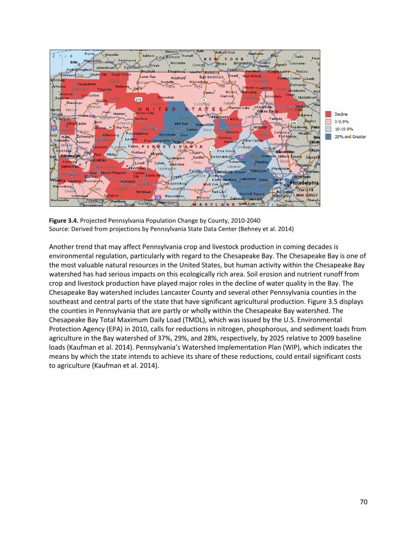
70

Figure 3.4. Projected Pennsylvania Population Change by County, 2010-2040 Source: Derived from projections by Pennsylvania State Data Center (Behney et al. 2014) Another trend that may affect Pennsylvania crop and livestock production in coming decades is environmental regulation, particularly with regard to the Chesapeake Bay. The Chesapeake Bay is one of the most valuable natural resources in the United States, but human activity within the Chesapeake Bay watershed has had serious impacts on this ecologically rich area. Soil erosion and nutrient runoff from crop and livestock production have played major roles in the decline of water quality in the Bay. The Chesapeake Bay watershed includes Lancaster County and several other Pennsylvania counties in the southeast and central parts of the state that have significant agricultural production. Figure 3.5 displays the counties in Pennsylvania that are partly or wholly within the Chesapeake Bay watershed. The Chesapeake Bay Total Maximum Daily Load (TMDL), which was issued by the U.S. Environmental Protection Agency (EPA) in 2010, calls for reductions in nitrogen, phosphorous, and sediment loads from agriculture in the Bay watershed of 37%, 29%, and 28%, respectively, by 2025 relative to 2009 baseline loads (Kaufman et al. 2014). Pennsylvania’s Watershed Implementation Plan (WIP), which indicates the means by which the state intends to achieve its share of these reductions, could entail significant costs to agriculture (Kaufman et al. 2014).

71

Figure 3.5. Pennsylvania counties in the Chesapeake Bay Watershed Source: Chesapeake Bay Program (2008)

3.3.2 Demand and markets Pennsylvania is part of local, regional, national, and global markets for food and agricultural products. In some cases, such as hay and certain seasonal fruits and vegetables, prices are determined on local and regional markets. Changes in demand or supply within Pennsylvania will affect prices facing farmers, consumers and others in the supply chain. In other cases, such as dairy products and mushrooms, prices are determined on national and global markets but Pennsylvania is a large enough producer of these products that changes in supply within the state will have a noticeable impact on markets. In still other cases, such as corn and soybeans, prices are determined on global markets, and Pennsylvania has such as small share of the global market that what happens within the state has no significant impact on market prices. One important trend in recent years has been rapidly growing demand for organic products. Organic product sales now represent more than 4% of total U.S. food sales (USDA, Economic Research Service 2014c). Fresh fruits and vegetables account for 43% of organic food sales, followed by dairy products (15%), packaged and prepared foods (11%), beverages (11%), bread and grains (9%), snack foods (5%), meat, fish and poultry (3%), and condiments (3%) (USDA, Economic Research Service 2014c). The US organic food market is expected to increase 14% per year during 2013-2018, while the non-organic food market is only expected to grow by 3% per year. Pennsylvania is geographically well-positioned to supply this increased demand for organic products due to proximity to major population centers. The result of the growing demand for organic products combined with technological change through biotechnology could split Pennsylvania agriculture into two production systems: one heavily invested in biotechnology, and one organic. In some cases, the same farm is part of both systems, with organic and non-organic agriculture in different fields.

72

Another trend that is becoming important is growing demand for local foods—foods produced within the consumer’s county or state, depending on the definition of “local.” There are few reliable statistics on market shares of local foods. Low and Vogel (2011) estimate that local food sales were about $5 billion in 2008, which was less than 1% of U.S. retail food sales. To the extent that the trend toward local foods continues, there will be a growing demand by Pennsylvania consumers for Pennsylvania food and agricultural products, particularly fresh fruits and vegetables. Projections of world market prices for agricultural commodities in coming decades depend on the assumptions made about global demand relative to global supply. In the near term, the USDA’s agricultural baseline projections for 2014-2023 indicate that prices for major crops are likely to recover somewhat from their recent drops, increasing gradually over time and remaining above pre-2007 levels (USDA, Office of the Chief Economist 2014). Prices for livestock products are also projected to increase gradually over most of this period. Beyond the mid-2020s, the uncertainties involved in agricultural market projections—including uncertainties about population growth, income growth, technological change, land and water availability, energy markets and biofuels, and agricultural policies—become far greater. Ray et al. (2013) expect that global food demand will increase by an average of 2.4% per year through 2050, but they project that yield increases for corn, rice, wheat and soybeans will only range from 0.9% to 1.6% per year. If this happens, commodity prices may be subject to strong market pressures. On the other hand, projections to 2050 by the UN’s Food and Agriculture Organization (FAO) indicate that the growth rate in global food demand will only be about 1.1% per year through 2050, due to lower rates of population growth and more people reaching a satiation point in food consumption (Alexandratos and Bruinsma 2012). As a result, FAO projects that global agricultural supplies will keep pace with growth in global food demand. Beyond 2050, the uncertainties rise by another order of magnitude because of the possibility of technological changes that lead to a dramatic transformation of the agricultural sector. It seems likely that the agriculture of Pennsylvania and the world in 2100 will bear only a faint resemblance to that of today.

3.4 Climate change impacts The climate projections in Section 2 of this report indicate that annual mean temperatures in Pennsylvania may increase between 2.5ºF and 6.5ºF by mid-century (2041-2070), depending on the climate scenario and model employed. These increases are not projected to vary significantly by season. The climate models also project increases in average annual precipitation in Pennsylvania on the order of 10% by mid-century. Increases in precipitation are projected to occur throughout the year, with somewhat larger increases in the winter (around 15%) than the summer (around 5%). Thus, by the middle of the century, the climate of Pennsylvania is projected to be significantly different and agricultural production systems will have to adapt to a changing climate. To help understand how changes in climate can affect field crop production systems, we summarize in Table 2.1 the expected impacts, coarsely classified as positive and negative. Table 2.1 includes the effects of atmospheric carbon dioxide (CO2) concentrations, which have been increasing steadily since the onset of the industrial revolution.

73

Table 2.1. Summary of the effects of precipitation, temperature and carbon dioxide on plant growth and yield and other characteristics of field crop production systems in Pennsylvania

Factor Positive effects Negative effects Increases in average precipitation

- Alleviates summer drought - May increase forage and grain

yield

- Augmented runoff and risk of erosion and nutrient leaching

- Higher plant disease pressure

Increases in precipitation variability

- Increased risk of flooding - Difficulties planting crops timely - Longer dry spells may cause water stress - Increased demand for irrigation

Increases in average temperature

- Longer growing season and higher yield potential for summer crops

- Possible to expand double cropping beyond southeast Pennsylvania

- Possible to include new crops from warmer locations

- Higher chances successfully establishing cover crops

- Warmer nights may increase respiratory losses and may limit gains from warmer daytime temperatures

- Warmer springs may reduce yield of small grains if warming occurs during the grain filling phase

- Favorable conditions for pest insects and diseases

- Weeds from warmer climates expanding into Pennsylvania

- Possible increase in agrochemical load to deal with pests and weeds

Increases in extreme temperatures

- Heat stress in particular can neutralize gains from warmer temperature

- High risk for grain crops or fruits crops (grapes) that flower in summer months

Increases in CO2 concentration

- Increase in productivity, particular for cool season plants and non-grasses summer plants (soybean)

- Increased water use efficiency

- Rarely, an enhancement of heat stress if temperatures are extreme, seems unlikely in Pennsylvania

Higher winter and summer temperatures both affect crop production systems, but the main shift may be caused by milder winters and earlier warming during spring. The temperature during the spring, summer and fall controls the potential length of the crop life cycle. Pennsylvania is in a transitional location, with southeastern Pennsylvania suitable for medium length maturity types in corn, but relatively short cycles in the northwest part of the state. Warmer summers may require using longer season corn hybrids (higher relative maturity) to capitalize on a longer growing season. Most of the benefit would come from earlier planting, when the solar radiation load is high but air and soil temperatures are (currently) suboptimal. Thus, a gradual shift to earlier planting dates for summer crops can be expected. There are many genetic options for corn, as well as for soybeans, to accommodate this earlier planting. Higher average temperatures may also allow the expansion of double cropping, which is currently practiced only on a limited basis in southeastern Pennsylvania (winter barley – soybeans). Double cropping may add dynamism to Pennsylvania agriculture, but also require changes in supply

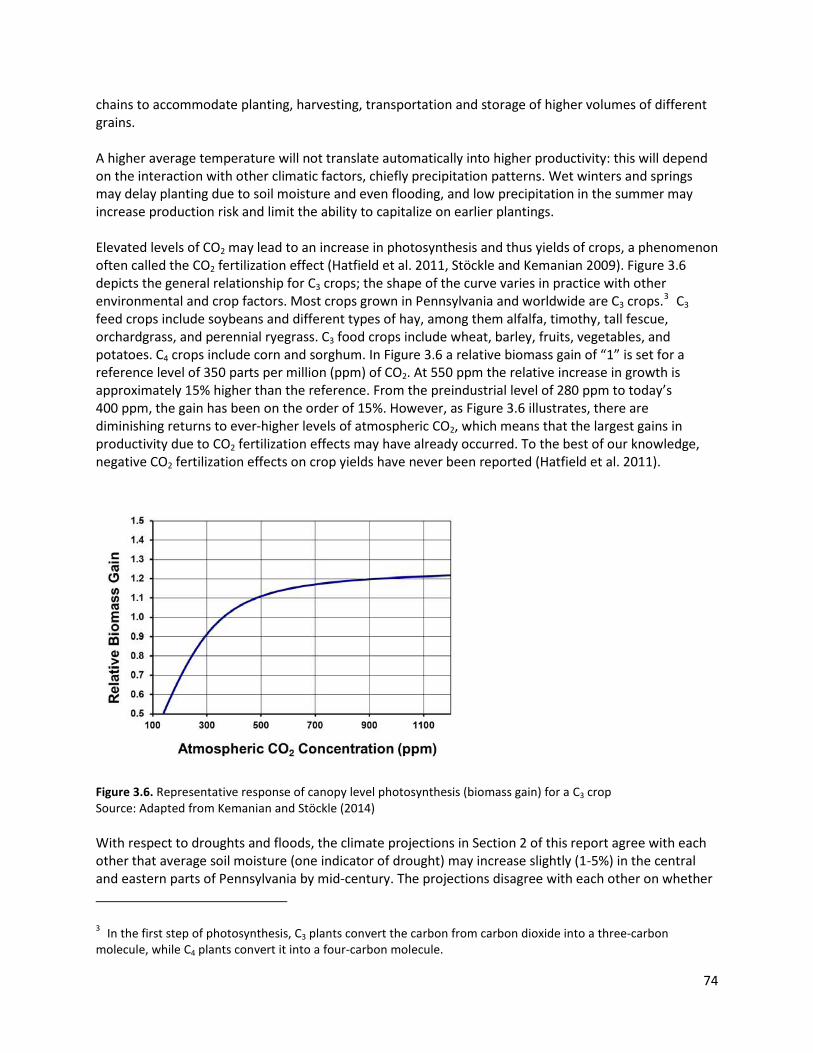
74

chains to accommodate planting, harvesting, transportation and storage of higher volumes of different grains. A higher average temperature will not translate automatically into higher productivity: this will depend on the interaction with other climatic factors, chiefly precipitation patterns. Wet winters and springs may delay planting due to soil moisture and even flooding, and low precipitation in the summer may increase production risk and limit the ability to capitalize on earlier plantings. Elevated levels of CO2 may lead to an increase in photosynthesis and thus yields of crops, a phenomenon often called the CO2 fertilization effect (Hatfield et al. 2011, Stöckle and Kemanian 2009). Figure 3.6 depicts the general relationship for C3 crops; the shape of the curve varies in practice with other environmental and crop factors. Most crops grown in Pennsylvania and worldwide are C3 crops.3 C3 feed crops include soybeans and different types of hay, among them alfalfa, timothy, tall fescue, orchardgrass, and perennial ryegrass. C3 food crops include wheat, barley, fruits, vegetables, and potatoes. C4 crops include corn and sorghum. In Figure 3.6 a relative biomass gain of “1” is set for a reference level of 350 parts per million (ppm) of CO2. At 550 ppm the relative increase in growth is approximately 15% higher than the reference. From the preindustrial level of 280 ppm to today’s 400 ppm, the gain has been on the order of 15%. However, as Figure 3.6 illustrates, there are diminishing returns to ever-higher levels of atmospheric CO2, which means that the largest gains in productivity due to CO2 fertilization effects may have already occurred. To the best of our knowledge, negative CO2 fertilization effects on crop yields have never been reported (Hatfield et al. 2011).

Figure 3.6. Representative response of canopy level photosynthesis (biomass gain) for a C3 crop Source: Adapted from Kemanian and Stöckle (2014) With respect to droughts and floods, the climate projections in Section 2 of this report agree with each other that average soil moisture (one indicator of drought) may increase slightly (1-5%) in the central and eastern parts of Pennsylvania by mid-century. The projections disagree with each other on whether

3 In the first step of photosynthesis, C3 plants convert the carbon from carbon dioxide into a three-carbon molecule, while C4 plants convert it into a four-carbon molecule.

75

average soil moisture in western Pennsylvania will increase slightly or decrease slightly. The climate projections indicate that most occurrences of drought by mid-century are anticipated to occur in the autumn, which is opposite the historical trend in which the most frequent wet months have been in September-October. The projections also indicate a rise in the number of very wet months when precipitation is greater than 150% of the current average. In sum, Pennsylvania’s hydrological climate may become more extreme in the future. Extreme events tend to affect entire regions rather than isolated farms, thus causing volatility in local prices due to sudden reductions in forage production or grain supplies, a critical component of the dairy industry. Pennsylvania agriculture will be impacted not only by changes in its own climate but also by changes in climate in other agricultural production regions of the nation and world (Abler and Shortle 2000). These are indirect effects of climate change. As national and global agricultural markets adjust to these changes in production, commodity prices facing Pennsylvania farmers could change. As discussed in other sections of this report, climate change may also have impacts on nonagricultural sectors of the Pennsylvania economy, and economies of other states and countries. These changes might manifest themselves as changes in prices of purchased inputs used by Pennsylvania farmers, in competing demands for land within Pennsylvania, or alternative employment opportunities available to Pennsylvania farmers. Indirect impacts such as these are important because they can amplify or counteract direct impacts of climate change within Pennsylvania, and they may even have greater consequences for Pennsylvania agriculture than the direct impacts (Abler et al. 2000). The recent IPCC report on food security and food production systems (Porter et al. 2014) finds that it is very likely that changes in temperature and precipitation, without considering CO2 fertilization effects, will lead to increased global food prices by 2050. Estimated price increases range from 3% to 84%. This report also concludes that the combined effect of climate change and CO2 fertilization is about as likely to decrease global food prices as it is to increase them, with projected price changes ranging from -30% to +45%. Some studies have used what is known as a Ricardian approach to analyze the impacts of climate change on county-level agricultural land values. The Ricardian approach is based on the idea that the value of a parcel of land capitalizes the discounted value of all future profits or rents that can be derived from the land, and that these profits or rents may be impacted by changes in temperature and precipitation. The first study to use a Ricardian approach (Mendelsohn et al. 1994) found that the effects of climate change on agricultural land values in Pennsylvania counties might range from small negatives to small positives, with the southern counties in Pennsylvania more likely to see negatives and the northern counties more likely to see positives. A study by Schlenker et al. (2006) reached similar conclusions. A recent study by Massetti and Mendelsohn (2011) analyzed county-level data but reported results for broad regions of the country. For the Northeast region, which includes Pennsylvania, they found that climate change is likely to increase agricultural land values. Warming and CO2 fertilization effects may promote the growth of weeds, limiting yield increases for crops and/or leading farmers to apply more herbicides or do more mechanical weeding. Most of the worst weeds worldwide are C4 plants, although many weeds currently affecting Pennsylvania agriculture are C3 plants, including common lambsquarters, common ragweed, velvetleaf, and common chickweed. Warming can be expected to lead to a northern expansion of tropical and other warm-season weeds. Crop-weed interactions are complex, and one cannot say whether climate change and CO2 fertilization effects will favor crops relative to weeds or vice versa (Pritchard and Amthor 2005, Porter et al. 2014). However, some changes seem to be already at work. As recently as 2013, Palmer Amaranth, a weed

76

related to other Amaranth spp. (pigweed), has been found for the first time in several locations in Pennsylvania. It is hard to argue that the northward expansion of this weed happened because of warming, but warmer and wetter conditions definitely favor its occurrence. Resistance to glyphosate has been reported for this species (Curran and Lingenfelter 2014). Warming may lead to a northern expansion of plant parasitic nematodes, and insects, presenting Pennsylvania agriculture with a different set of pest challenges than it faces today. Warming may also increase populations of marginally overwintering insect species such as corn flea beetles (Wolfe et al. 2008). On the other hand, if droughts become more frequent, the pressure and spread of many insects could decline (Wolfe et al. 2008). Natural enemies of crop pests such as birds and beneficial insects might benefit from a warmer climate (Pritchard and Amthor 2005). It is difficult to say whether climate change will favor crop pests relative to birds and beneficial insects, or vice versa (Porter et al. 2014; DeLucia et al. 2012). Warming is likely to lead to phenological advances in a variety of plants, birds, and insects (Richardson et al. 2013). Insect pests may develop more quickly in a warmer climate, and multivoltine insects might be able to complete more life cycles during a year (Pritchard and Amthor 2005; DeLucia et al. 2012). Warming in the northeast U.S. over the past 130 years has advanced the phenology of spring-active bees by about 10 days, tracking earlier blooming (Bartomeus et al. 2011). More research is needed on how agriculture in general, and Pennsylvania agriculture, is likely to be affected by phenological changes. A review of the literature on crop diseases and climate change by Newton et al. (2011) concluded that complex biological interactions among pests, pathogens, mutualists, and parasites can lead to outcomes that differ from those predicted from the responses of each individual organism to temperature, precipitation, or atmospheric CO2. A review of the literature on climate change and invasive species (pathogens, insects and weeds) by Ziska et al. (2011) identified a number of research gaps and concluded that the research to date is inadequate to characterize the impacts of climate change on invasive species beyond the micro scale (e.g. beyond the scale of a leaf). The evolving weed and insect management challenges created by climate change may lead farmers to apply different types of pesticides, and in different quantities, than today. Whether these changes will be beneficial or harmful for the environment is unclear. It is possible that genetic engineering during coming decades may improve the pest resistance of crops to the point where insecticide usage is significantly reduced, just as insect-resistant (Bt) hybrids of corn to control the corn borer and corn rootworm are already on the market. However, new pest populations and the constant development of resistance among pests (e.g. Gassmann et al. 2011) may require an intensification of agricultural management, particularly if benign winters allow some plague insects to establish resident populations. Organic agriculture may help farmers adapt to climate change because the labor-intensive nature of these systems allows for product diversification. However, organic agriculture by definition relinquishes the use of transgenic products and most forms of synthetic agrochemical use. A warmer climate may make organic agriculture more vulnerable to pests and diseases, although the activity of natural predators may also increase, helping to control problem insects. Area suppression of pest insect by non-organic agriculture (Hutchison et al. 2011) may help ameliorate potential increases in insect pressures. Good stewardship of the soil in organic agriculture that increases soil organic matter may cause soils to retain significantly more rainwater (Niggli et al. 2007) and minimize the effect of excess precipitation or dry spells. Organic, grass fed livestock production may increase due to a longer growing season, capitalizing on a growing segment of the market.

77

Any future increases in the variability of temperature and precipitation in Pennsylvania are likely to increase the demand by farmers for risk management products, including insurance against losses due to drought, flooding, hail, wind, frost, insects, and disease. Federal crop insurance is heavily subsidized, with the federal government paying over 60% of premium costs (GAO 2014). There are a wide variety of insurance options for crop producers, including hail insurance, multiple peril yield insurance, market price insurance, and revenue insurance.

3.4.1 Feed crops Statistics from the 2012 Census of Agriculture indicate that the three most important feed crops in terms of acreage in Pennsylvania are hay, corn (for grain and for silage), and soybeans, and the most important in terms of sales are corn and soybeans. This section focuses on these crops. Southeastern Pennsylvania currently has good conditions for corn production. Nighttime temperatures are relatively high but daytime temperatures are excellent for this C4 crop. The current climate in the northern and western parts of the state is slightly more marginal for corn, as increases in elevation reduce temperatures and the length of the growing season. Some insight into the potential impacts of climate change on corn production in Pennsylvania can be gleaned from a recent simulation modeling study of corn yield responses to warming and CO2 in two temperate locations that bear some resemblance to Pennsylvania (Iowa and Lusignan, France), and two warm locations (subtropical Brazil and Tanzania) that serve as points of contrast (Bassu et al. 2014). This study finds that increases in CO2 can increase corn yields modestly in temperate locations. This study also finds that temperature increases reduce yields in the warm locations, and in the temperate locations when the increase is extreme (+10°F or greater). However, modest increases in temperature increase corn yields in the temperate locations. In both Lusignan and Iowa, the yield increase is a response to higher temperatures in early spring and fall, which allows crops more time to mature and express their full yield potential. Translating this to Pennsylvania, the implication is that corn yields may increase slightly in central and northern Pennsylvania, provided that water availability does not limit yield expression. Figures 3.7 and 3.8 illustrate results from the study by Bassu et al. (2014). Figure 3.7 presents a box-and-whisker plot of the 30-year average response of grain yields (in %) to CO2 as simulated by 15 different models. Figure 3.8 is like Figure 3.7, except that 3.8 shows the response of grain yields to higher temperatures. The upper and lower lines on the boxes show the 25th and 75th percentiles of yield responses, with the line in the middle of each box show the median yield response. The whiskers show the 10th and 19th percentiles, and the hollow circles indicate outliers. In a statistical analysis of U.S. yields for corn, soybeans, and cotton, Schlenker and Roberts (2009) found that corn yields increase slightly with average temperature during the growing season up to an average of about 84ºF, beyond which yields decline significantly. They found a similar pattern for soybeans, with a threshold of about 86ºF beyond which yields decline with higher temperatures regardless of other factors. The average historical (1971-2000) growing season temperature for corn and soybeans in southeastern Pennsylvania (climate division 3, which includes Lancaster County) is about 66ºF, which is well below the thresholds identified by Schlenker and Roberts (2009). Average historical growing season temperatures in the central and northern regions of Pennsylvania are even lower. This study implies that moderate warming may increase Pennsylvania corn and soybean yields, provided that water availability is not limiting.

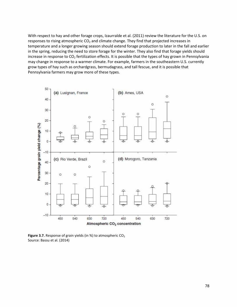
78

With respect to hay and other forage crops, Izaurralde et al. (2011) review the literature for the U.S. on responses to rising atmospheric CO2 and climate change. They find that projected increases in temperature and a longer growing season should extend forage production to later in the fall and earlier in the spring, reducing the need to store forage for the winter. They also find that forage yields should increase in response to CO2 fertilization effects. It is possible that the types of hay grown in Pennsylvania may change in response to a warmer climate. For example, farmers in the southeastern U.S. currently grow types of hay such as orchardgrass, bermudagrass, and tall fescue, and it is possible that Pennsylvania farmers may grow more of these types.

Figure 3.7. Response of grain yields (in %) to atmospheric CO2 Source: Bassu et al. (2014)

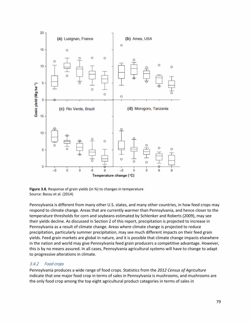
79

Figure 3.8. Response of grain yields (in %) to changes in temperature Source: Bassu et al. (2014) Pennsylvania is different from many other U.S. states, and many other countries, in how feed crops may respond to climate change. Areas that are currently warmer than Pennsylvania, and hence closer to the temperature thresholds for corn and soybeans estimated by Schlenker and Roberts (2009), may see their yields decline. As discussed in Section 2 of this report, precipitation is projected to increase in Pennsylvania as a result of climate change. Areas where climate change is projected to reduce precipitation, particularly summer precipitation, may see much different impacts on their feed grain yields. Feed grain markets are global in nature, and it is possible that climate change impacts elsewhere in the nation and world may give Pennsylvania feed grain producers a competitive advantage. However, this is by no means assured. In all cases, Pennsylvania agricultural systems will have to change to adapt to progressive alterations in climate.

3.4.2 Food crops Pennsylvania produces a wide range of food crops. Statistics from the 2012 Census of Agriculture indicate that one major food crop in terms of sales in Pennsylvania is mushrooms, and mushrooms are the only food crop among the top eight agricultural product categories in terms of sales in

80

Pennsylvania.4 Mushroom sales in 2012 were about $530 million. Important food crops in Pennsylvania also discussed in this section are fruits, tree nuts and berries (sales of $161 million) and vegetables, melons and potatoes (sales of $141 million). Mushrooms are almost entirely cultivated inside of specialized growing houses under carefully controlled temperature and humidity, with different temperatures required depending on the stage of the cultivation process and the type of mushroom being produced. Humidity is generally maintained at a high level throughout the process, which can take roughly three months from preparation of the compost in which the mushrooms are grown through to harvesting. There are no firm statistics for Pennsylvania, but statistics for the U.S. as a whole suggest that less than 5% of mushroom sales come from mushrooms grown outdoors in the woods (USDA, National Agricultural Statistics Service 2008). There are also a few mushroom farms in limestone caves or abandoned coal mines, but these are generally considered unreliable because of the difficulty of controlling climatic conditions. The effects of climate change on mushroom production will primarily be manifested in changes in heating and cooling requirements for growing houses. As part of the preparation process, compost is pasteurized at about 140°F for two hours or more in order to eradicate harmful bacteria, nematodes, insects, and fungi. Higher average outdoor temperatures will lower heating requirements during the pasteurization process. Because multiple crops of mushrooms can be grown and harvested indoors during a single year, the effects of climate change on other stages of the mushroom growing process will depend on the season in which the mushrooms are being grown. Many temperate mushrooms require ambient temperatures of 70-80ºC during the spawning and growth stage, which typically lasts 2-3 weeks. With climate change, there will on average be less heating required during the winter months but additional cooling during the summer months. The net effects on annual energy use and annual production costs are unclear. For fruits and vegetables, an increase in summer heat stress may be damaging to cool temperature-adapted crops such as apples and potatoes (Wolfe et al. 2008). Fruits such as apples and grapes have a winter chilling requirement of 200-2,000 cumulative hours within a narrow temperature range, typically 32-50ºF (Wolfe et al. 2008; Luedeling 2012). Temperatures outside of this range generally do not meet this chill requirement. Among grapes, native American varieties (Vitis labruscana) have a much longer chilling requirement than European varieties (Vitis vinifera) (Wolfe et al. 2008). European varieties, by contrast, do poorly if temperatures drop below about 15ºF during the winter. In a warmer climate, Pennsylvania wineries may choose to replace some of their native American grape varieties with European varieties. This would entail costs in removing current vines and replanting them with new ones. It would entail benefits because wines from European varieties generally command higher prices than those from American varieties. An increase in the frequency of floods and droughts may be damaging to fruits and vegetables that are vulnerable to quality defects, such as blossom end rot in tomato, caused by hourly and daily fluctuations in water availability (Wolfe et al. 2008). Wetter summers and falls, with the associated increase in cloudiness, may also limit the quality of the fruit. Quality is important for any crop but particularly so for fresh fruits and vegetables, where blemishes or defects may significantly lower the price received or

4 The top-eight list in order of sales, as mentioned above, is: dairy; poultry and eggs; corn; cattle and calves; mushrooms; other nursery and greenhouse products (aside from mushrooms); hogs and pigs; and soybeans. These eight product categories account for 89% of total agricultural product sales in Pennsylvania.

81

even render the product unsalable. At the same time, because fruits, vegetables and potatoes are C3 crops, the CO2 fertilization effect may at least partially offset yield declines due to changes in temperature and precipitation. However, as noted above, most of the yield gains from atmospheric CO2 increases may have already been accrued. Warmer temperatures and longer growing seasons may permit Pennsylvania food crop producers to grow more of crops such as sweet corn that are well suited to these conditions. Pennsylvania sweet corn producers may be able to deliver their product to market earlier in the year, increasing their competitiveness with corn grown in southern states that have traditionally dominated the early summer market for sweet corn. Wheat is not a major crop in Pennsylvania ($64 million in sales in 2012), but the potential effects of CO2 and climate change on wheat have been studied extensively because of the importance of wheat worldwide. Wheat and other C3 small grains have a higher responsiveness to CO2 than corn (a C4 crop). Small grains also differ from corn because their grain filling occurs in a narrow time window after flowering. Reductions in the length of grain filling due to increased temperatures (and therefore reductions in the total radiation interception) may limit yield gains from other factors. Asseng et al. (2013) assembled simulations from 20 models for four locations worldwide (Netherlands, Argentina, India, Australia) changing both CO2 and temperature. The results are illustrated in Figure 3.9. None of the four locations is clearly analogous to the climate in Pennsylvania, but yields in each location are highly responsive to temperature. Warmer winters may allow double cropping of small grains, perhaps short cycle winter barley or oats rather than winter wheat (unless the winters are wet, which is not favorable for barley).

82

Figure 3.9. Sensitivity of simulated and observed wheat yields to temperature and CO2 Note: Simulated relative mean (30-year average, 1981–2010) grain yield change for increased temperatures (no change, grey; +3 °C (5.4°F), red; +6 °C (10.8°F), yellow) and elevated atmospheric CO2 concentrations for the Netherlands (NL; a), Argentina (AR; b), India (IN; c) and Australia (AU; d). For each box plot, vertical lines represent, from left to right, the 10th percentile, 25th percentile, median, 75th percentile, and 90th percentile of simulations based on 20 models). Inset: Observed range of yield impacts with elevated CO2. Source: Asseng et al. (2013)

3.4.3 Other crops Statistics from the 2012 Census of Agriculture indicate that annual Pennsylvania sales of other nursery and greenhouse products (aside from mushrooms) are $415 million, making it one of the top eight agricultural product categories in terms of sales in Pennsylvania. The two most important products within this category are bedding/garden plants ($141 million in sales) and nursery stock ($126 million in sales). Other important products include potted plants, greenhouse tomatoes, and cut flowers.

83

For bedding/garden plants and nursery stock, climate change is likely to necessitate changes in the types of species that are grown and sold to consumers. There is unlikely to be a significant threat to the economic health of the industry—there will still be a demand for landscaping products in a warmer climate, just as there is in southern states today. The USDA’s Plant Hardiness Zone Map was last updated in 1990, but the Arbor Day Foundation released its own updated map in 2006 showing that parts of many states have shifted by one hardiness zone since 1990 and some areas have shifted by two zones. Commercial nurseries can facilitate climate change adaptation by providing a head start for northward range shifts among plant species (Van der Veken et al. 2008). For greenhouse tomatoes, it is hard to find locations in the U.S. where the climate makes production profitable in both the summer and winter (Cook and Calvin 2005). Currently there is significant winter greenhouse tomato production only in the west and southwest parts of the country. If winter temperatures rise significantly due to climate change, greenhouse heating costs in Pennsylvania might fall to the point where it becomes profitable to produce greenhouse tomatoes in the winter. Climate permitting, winter greenhouse production is more profitable than summer production because tomato prices are significantly higher in the winter (Cook and Calvin 2005). The question in this case is whether summer production would continue to be profitable in the face of higher summer temperatures. Moreover, heating costs for winter greenhouse tomatoes grown in other states would also fall, putting downward pressure on market prices.

3.4.4 Livestock products Statistics from the 2012 Census of Agriculture indicate that four livestock products are among the top eight agricultural product categories in Pennsylvania in terms of sales: dairy, poultry and eggs, cattle and calves, and hogs and pigs. This section focuses on these livestock products. Like all warm-blooded animals, livestock require ambient temperatures that allow them to maintain a body temperature within narrow bounds (Boesch 2008), in most cases above ambient temperature. If the heat losses outpace the metabolic heat production and the energy gained from the environment (for example radiation from sunlight), they have to increase the metabolic rate to match the energy losses and preserve an operative body temperature. If the environment is hot the animal must seek conditions that avoid heat stress, typically seeking shade and increasing panting. These situations increase stress and reduce the energy that can be devoted to production of products such as milk, bodily growth, and reproduction. As an animal’s productivity increases, whether it is higher milk yields for dairy cows or faster growth rates for pigs or poultry, metabolic heat production also increases and the capacity to tolerate high temperatures decreases (Porter et al. 2014). Heat stress can lead to reduced physical activity, reduced eating or grazing, higher mortality, and lower fertility (Nardone et al. 2010). Temperature thresholds vary according to the species of livestock and each individual animal’s genetics and health. In Pennsylvania dairy and beef cattle production, livestock are outdoors much of the time. Dairy cows prefer cool temperatures, with the optimum temperature range for milk production being roughly 40-75°F (Wolfe et al. 2008). Using climate model projections indicating that U.S. dairy production areas will experience annual temperature increases of about 1.5-2.4°F by 2030, Key et al. (2014) estimate that milk production at the average Pennsylvania dairy could decline by about 0.6% to 0.9%. Larger increases in the average summer temperature of 9-11°F could lead to heat stress losses of 10-25% in milk production (Wolfe et al. 2008). Beef cattle have a somewhat greater tolerance than dairy cows for heat, but large increases in the average summer temperature could place significant heat stress on them as well.

84

Dairy and beef cattle producers can reduce heat stress by providing trees, buildings, or portable shelters for shade. They can also use fans and spray water on their cattle to help keep them cool. However, these actions are not free. One indicator of the cost of alleviating heat stress in dairy cattle is energy expenditures per hundredweight (100 pounds) of milk produced. Figure 3.11, from Key et al. (2014), illustrates how energy expenditures per hundredweight increase as the level of heat stress increases. This increasing relationship between heat stress and energy expenditures is true for dairies of all sizes (small, medium, and large). Dairy producers can also adapt to heat stress by switching breeds. For example, Jerseys have smaller declines in milk production than Holsteins in response to heat stress, and consequently dairies in the highest heat stress regions of the U.S. have the greatest share of Jersey cows in their herds (Key et al. 2014).

Figure 3.11. Energy expenditures by dairies and heat stress Source: Key et al. (2014) Poultry and eggs in Pennsylvania are mostly produced in large-scale indoor facilities where the birds are kept in close quarters. Housing large numbers of birds with a high metabolism makes them vulnerable to heat stress during the summer (Boesch 2008). Birds can be at least partially protected against heat stress through investments in insulation, ventilation, fans and air conditioning in growing facilities. The existence of large-scale poultry production in southern states such as Alabama, Arkansas, Georgia, and Mississippi indicate that these investments can be made at acceptable cost, at least with current energy prices. Higher energy prices might change that calculation.

85

Adult hogs prefer cooler temperatures, with the optimum temperature range for adult hog growth being 55-70°F. Baby pigs must be kept warmer, with optimum temperatures between 85-90°F. Hogs and pigs in Pennsylvania are typically housed inside of growing facilities, with ventilation and fans used to keep hogs cool during the summer. During very high summer temperatures, producers will sometimes spray water on their hogs to keep them cool. With climate change, heating costs may fall during warmer winters but costs of keeping animals cool during the summer may rise. The net effect on annual energy use and annual production costs are unclear. However, the existence of large-scale hog production in southern states such as North Carolina and Oklahoma suggests that Pennsylvania hog production is likely to continue being economically viable in a warmer climate. Currently, a large portion of poultry and hog production is concentrated in warmer, more southern states. These operations were originally located in these states when energy prices and average temperatures were lower than they are today. The concentration may have occurred due to a clustering effect, since these sectors depend highly on the availability of specialized products and services that can be supplied more efficiently to a large number of farms than a small number. Since climate control is a substantial input into the growth of these livestock, climate change may stimulate the movement of poultry and hog production northward into states like Pennsylvania (Abler et al. 2009). Given the highly clustered nature of these industries, the movement could be large-scale rather than incremental. Large-scale poultry and hog production serves as a nutrient concentrator on the landscape because a large proportion of the nutrients in feed are spread on land near the animal facilities in the form of manure, typically creating high phosphorus concentrations in the topsoil that act as a pollution source. A northward movement of such industries could create a tension for Pennsylvania between economic benefits and environmental protection. There may also be a northward movement of dairy production in response to climate change, but a large-scale movement is not possible simply because there is relatively little dairy production in southern states to move. This is one reason why Key et al. (2014) project milk production losses in response to climate change in all the states they examine, including Pennsylvania, although Pennsylvania’s losses in percentage terms are much lower than states such as Florida and Texas. Climate change is also likely to impact livestock production through parasites, pathogens, and disease vectors (Boesch 2008). As discussed earlier, there may be northward migration of livestock pests currently found in southern states and greater overwintering of pests already present in Pennsylvania. Pennsylvania livestock producers will likely face a different set of pest and disease management challenges than they face today, but we cannot say whether the challenges will be greater or smaller. Pennsylvania livestock production may also be impacted by climate change through changes in forage production and quality, on-farm production of feed crops, and changes in prices of purchased feed. As discussed earlier, projected increases in temperature and a longer growing season should extend forage production to later in the fall and earlier in the spring, reducing the need to store forage for the winter. Forage yields may also increase in response to increases in precipitation and CO2 fertilization effects. On the other hand, increased precipitation, particularly during spring, may make grazing more challenging as the ground may be wet and pastures can be damaged by trampling. Research on the effects of changes in temperature and precipitation on forage quality has yielded conflicting results (Craine et al. 2010). Craine et al. (2010) used a long-term, national database of cattle fecal chemical composition to analyze the impacts of temperature and precipitation on crude protein (CP) and digestible organic matter (DOM) in forage crops. For forested regions with a climate similar to

86

Pennsylvania, they find that higher annual temperatures are associated with lower levels of CP and DOM. They do not report impacts of changes in precipitation for these regions.

3.5 Economic opportunities and barriers for Pennsylvania Adaptation to climate change, and efforts to mitigate greenhouse gas emissions, may create economic opportunities for Pennsylvania agriculture. One opportunity is alternative energy. The main energy crop in the U.S. is currently corn, which is used for ethanol. However, there are three reasons why this situation may change. First, the “blend wall” has been achieved (percentage of ethanol in the gasoline plus ethanol mix), meaning that additional ethanol can only be consumed if more gasoline is consumed; second, U.S. gasoline consumption is stable or decreasing due to better gas mileage in new vehicles; and third, with the “food versus fuel” debate, there is interest in substituting liquid fuels of lignocellulosic origin for corn-based ethanol. In light of this, there is an opportunity to make alternative, second-generation energy crops part of the agricultural landscape of Pennsylvania (U.S. Department of Energy 2011). Candidates include perennial shrub willow (Smart and Cameron 2008), a short rotation woody crop (and a C3 plant); the perennial grasses miscanthus and switchgrass (both C4 plants) (Khanna et al. 2008); and annuals such as biomass sorghum (Mullet et al. 2012) or winter rye, which is already grown as a cover crop. Other annuals include oil crops, which could supply feedstock for companies producing jet fuel. The non-food oil crops that might fit the environment of Pennsylvania would likely need to be short-season winter crops similar to pennycress, which could be double cropped with minimal impact on grain production. Studies on pennycress are limited, but warming and a lengthening of the growing season may open a window for this option. The perennial energy crops shrub willow, miscanthus and switchgrass have potential in Pennsylvania, as illustrated in Figure 3.10 (Kemanian et al. 2013). There is willow acreage at an experimental stage in Pennsylvania, commercial plantations of willow in New York, and commercial acreage of miscanthus in northwest Pennsylvania. Switchgrass, a native grass, is also productive and is currently harvested in Pennsylvania and pelletized for multiple uses. While irregular precipitation may affect growth of perennial crops in some parts of the season, these energy crop are likely to benefit from warmer conditions (C4 crops) and from wetter conditions in spring and increasing atmospheric CO2, particularly the C3 shrub willow. These crops may play a role not only in the energy matrix, but also in ameliorating erosion and off-site pollution. Inputs of agrochemicals are low compared with annual crops, and target locations for planting include wet parts of the landscape and floodplains that are major contributors to surface and subsurface water pollution. When planted in sensitive parts of the landscape, these energy crops can act as dual purpose riparian buffers that produce biomass and protect the environment. Displacement of fossil fuels or corn-based ethanol by alternative energy crops can reduce greenhouse gas emissions (Dunn et al. 2013; Davis et al. 2012; Chesapeake Bay Commission, 2007). This is particularly the case if biomass production and energy yield are high, as is expected from perennial energy crops, or if energy crops are produced in niche periods in between annual crops (e.g. winter rye). If there are regulatory or market incentives for reducing greenhouse gas emissions, alternative energy crops would open up opportunities for Pennsylvania agriculture.

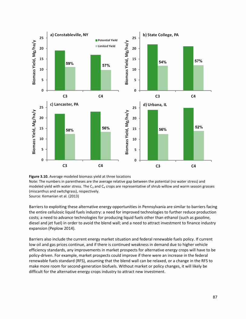
87

Figure 3.10. Average modeled biomass yield at three locations Note: The numbers in parentheses are the average relative gap between the potential (no water stress) and modeled yield with water stress. The C3 and C4 crops are representative of shrub willow and warm season grasses (miscanthus and switchgrass), respectively. Source: Kemanian et al. (2013) Barriers to exploiting these alternative energy opportunities in Pennsylvania are similar to barriers facing the entire cellulosic liquid fuels industry: a need for improved technologies to further reduce production costs; a need to advance technologies for producing liquid fuels other than ethanol (such as gasoline, diesel and jet fuel) in order to avoid the blend wall; and a need to attract investment to finance industry expansion (Peplow 2014). Barriers also include the current energy market situation and federal renewable fuels policy. If current low oil and gas prices continue, and if there is continued weakness in demand due to higher vehicle efficiency standards, any improvements in market prospects for alternative energy crops will have to be policy-driven. For example, market prospects could improve if there were an increase in the federal renewable fuels standard (RFS), assuming that the blend wall can be relaxed, or a change in the RFS to make more room for second-generation biofuels. Without market or policy changes, it will likely be difficult for the alternative energy crops industry to attract new investment.

88

In addition to energy crops, another opportunity for Pennsylvania agriculture for mitigating greenhouse gas emissions is storage of atmospheric CO2 in agricultural soils. Options for storing atmospheric carbon include conversion of cropland to forestry or pasture, planting of winter cover crops, reduced tillage practices, and planting energy crops on marginal agricultural land (Rosenzweig and Tubiello 2007). Estimates of the amount of carbon that might be sequestered by these options vary significantly (Rosenzweig and Tubiello 2007). Soil carbon storage is transient in the sense that stored soil carbon can be re-emitted depending on soil management (e.g. by turning cropland into pastureland and then back into cropland). The potential demand for land for installing solar photovoltaic (PV) arrays might affect agriculture, displacing some land from agricultural production but at the same time providing agricultural landowners the opportunity to earn income from selling or renting land. An increase the frequency of extreme weather events may have a negative effect on soil carbon sequestration if extreme events reduce production and therefore carbon inputs to the soil, which usually results in soil organic carbon losses (Kemanian and Stöckle 2010), or if extreme events increase the average soil moisture content and temperature, thereby increasing microbial soil respiration and CO2 emissions. Climate change may create an opportunity for Pennsylvania agriculture in the form of cover crops, because increases in average temperature improve the chances of successfully establishing cover crops. Cover crop challenges emerge from higher operational demands for both planting the cover crop and planting the crop that follows it, potential competition for water, demand for nitrogen (if grass cover crops), and cost. However, there are substantial environmental benefits for soil quality, reduction in erosion, retention of nutrients, habitat for natural predators, and pollination services (Schipanski et al. 2014). Cover crops can improve eight out of 11 ecosystems services without impacting negatively crop yields, and these benefits are expected to be retained or become more important under climate change (Schipanski et al. 2014).

3.6 Conclusions Pennsylvania agriculture can continue to prosper in a warmer climate, but changes will be required. Any producers who fail to adjust to climate change are likely to see their yields and profitability decline. Fortunately, Pennsylvania agriculture is an industry very familiar with continual and rapid change. An increase in the frequency of extreme events may require a higher level of intervention, flexibility and availability of production inputs for timely planting, harvesting and other operations. With regard to feed crops and feed cropping systems, it is likely that different hybrids of corn and varieties of soybean will need to be planted if growing seasons become longer and the weather more variable. A vast array of genetic options for these crops already exist as evidenced by their cultivation across a range of climatic conditions, but it will be necessary to identify and improve crop varieties specific to Pennsylvania’s future climate. While corn and soybean production are likely to remain dominant, the effects of climate change on the prevalence of alfalfa are uncertain. Alfalfa is a leguminous crop that fixes nitrogen in the soil. A reduction in the area of alfalfa may require shifting to other legumes or perhaps increased use of synthetic fertilizers. More investigation is necessary to determine how alfalfa yields and quality are likely to be impacted by climate change, and how these impacts will affect the rest of the crop mix. Once

89

again, the availability of a diverse set of species and genotypes within species seems critical to secure adaptability. With respect to the food crops that are grown in Pennsylvania, the effects of climate change on mushroom production are ambiguous. Yields of cool-temperature adapted fruits and vegetables such as potatoes and apples are likely to decline as a result of climate change, while yields of fruits and vegetables better suited to a warmer climate such as sweet corn are likely to rise. Pennsylvania farmers are likely to adapt to climate change by changing the types and varieties of fruits and vegetables grown. Pennsylvania wineries may choose to replace some of their native American grape varieties with European varieties. This would entail up-front costs in replacing vines but could be beneficial in the long run because wines from European varieties tend to command higher prices than wines from Native American varieties. For bedding/garden plants and nursery stock, climate change is likely to necessitate changes in the types of species that are grown and sold to consumers. There is unlikely to be a significant threat to the economic health of the industry—there will still be a demand for landscaping products in a warmer climate, just as there is in southern states today. The effects of climate change on Pennsylvania livestock producers are likely to be mixed. In the dairy industry, heat stress and a decline in feed quality are likely to drive milk yields downward and increase production costs. For operations that rely on grazing and on-farm production such as dairy and beef herds, changes in pasture yields and feed quality will impact production costs. For the state’s hog and poultry producers, while climate control costs are likely to increase with warmer summer months, this same effect in southern states may make Pennsylvania more attractive to these industries and could induce a northward shift in production operations. This may create a tension between the expansion of animal production and the ability of Pennsylvania to meet its water quality obligations under the Chesapeake Bay TMDL. Crop and livestock and producers are likely to encounter changing pest, weed, and disease management challenges. Just as a changing climate may require new crop and animal species in production, it may also make the environment suitable for different species of insects and weeds as well as types of disease. Improvements in crop and livestock genetics may ameliorate these issues. The main energy crop in the U.S. today is corn. If cellulosic energy crops become important in the future, they may benefit from warmer climate and help reduce the carbon footprint of agriculture. When the 2009 and 2011 versions of the Pennsylvania Climate Impact Assessment were written, there was limited information on energy crops in Pennsylvania. Today there are several trials with warm season grasses and shrub willow in the state and the Mid-Atlantic region. This is a dynamic area of research and development that holds promise for Pennsylvania agriculture.

References Abler, D.G., and Shortle, J.S. (2000). Climate change and agriculture in the Mid-Atlantic region. Climate

Research, 14 (3), 185–194. Abler, D., Shortle, J., Rose, A., and Oladosu, G. (2000). Characterizing regional economic impacts and

responses to climate change. Global and Planetary Change, 25 (1–2), 67–81.

90

Abler, D., Fisher-Vanden, K., McDill, M., Ready, R., Shortle, J., Sue Wing, I., and Wilson, T. (2009). Economic Impacts of Projected Climate Change in Pennsylvania. Report to Pennsylvania Department of Environmental Protection.

Alexandratos, N., and Bruinsma, J. (2012). World Agriculture towards 2030/2050: The 2012 Revision. ESA Working Paper No. 12-03, Food and Agriculture Organization. Retrieved from http://www.fao.org/docrep/016/ap106e/ap106e.pdf.

Bartomeus, I., Ascher, J.S., Wagner, D., Danforth, B.N., Colla, S., Kornbluth, S., and Winfree, R. (2011). Climate-associated phenological advances in bee pollinators and bee-pollinated plants. Proceedings of the National Academy of Sciences, 108 (51), 20645-20649.

Bassu, S, Brisson, N., Durand, J-L., Boote, K., Lizaso, J., Jones, J.W., Rosenzweig, C., Ruane, A.C., Adam, M., Baron, C., Basso, B., Biernath, C., Boogaard, H., Conijn, S., Corbeels, M., Deryng, D., DiSanctis, G., Gayler, S., Grassini, P., Hatfield, J., Hoek, S., Izaurralde, C., Jongschaap, R., Kemanian, A.R., Kersebaum, C.K., Kumar, N.S., Makowski, D., Müller, C., Nendel, C., Priesack, E., Pravia, M.V., Kim, S-H., Sau, F., Shcherbak, I., Tao, F., Teixeira, E., Timlin, D., and Waha, K. (2014). How do various maize crop models vary in their responses to climate change factors? Global Change Biology, 20 (7), 2301–2320.

Behney, M., Copella, S., Shultz, and J., Bowalick, D. (2014). Pennsylvania Population Projections 2010-2040. Report to the Center for Rural Pennsylvania. Retrieved from http://www.rural.palegislature.us/documents/reports/Population_Projections_Report.pdf.

Boesch, D.F. (editor) (2008). Global Warming and the Free State: Comprehensive Assessment of Climate Change Impacts in Maryland. Report of the Scientific and Technical Working Group of the Maryland Commission on Climate Change. University of Maryland Center for Environmental Science, Cambridge, Maryland.

Chesapeake Bay Commission (2007). Biofuels and the Bay: Getting It Right to Benefit Farms, Forests and the Chesapeake. Annapolis, MD: Chesapeake Bay Commission. Retrieved from http://www.chesbay.us/Publications/BiofuelsAndTheBay1.pdf

Chesapeake Bay Program (2008). Chesapeake Bay Counties. Retrieved from http://www.chesapeakebay.net/images/maps/cbp_297301.pdf.

Cook, R., and L. Calvin (2005). Greenhouse Tomatoes Change the Dynamics of the North American Fresh Tomato Industry. USDA, Economic Research Service, Economic Research Report No. 2. Retrieved from http://www.ers.usda.gov/media/307225/err2_1_.pdf.

Craine, J.M., Elmore, A.J., Olson, K.C., and Tolleson, D. (2010). Climate change and cattle nutritional stress. Global Change Biology, 16 (10), 2901–2911.

Curran, W.S., and Lingenfelter, D.D. (2014). Palmer Amaranth, a New Threat to Pennsylvania Agriculture. Penn State Cooperative Extension. Retrieved from http://extension.psu.edu/pests/weeds/herbicide-resistant-weed-information/palmer-amaranth-a-new-threat-to-pennsylvania-agriculture.

Davis, S.C., Parton, W.J., Del Grosso, S.J., Keough, C., Marx, E., Adler, P.R., and DeLucia, E.H. (2012). Impact of second-generation biofuel agriculture on greenhouse-gas emissions in the corn-growing regions of the US. Frontiers in Ecology and the Environment, 10, 69–74.

DeLucia, E.H., Nabity, P.D., Zavala, J.A., and Berenbaum, M.R. (2012). Climate change: Resetting plant-insect interactions. Plant Physiology, 160 (4), 1677–1685.

Dunn, J.B., Mueller, S., Kwon, H., and Wang, M.Q. (2013). Land-use change and greenhouse gas emissions from corn and cellulosic ethanol. Biotechnology for Biofuels, 6:51. Retrieved from http://www.biomedcentral.com/content/pdf/1754-6834-6-51.pdf.

GAO (U.S. Government Accountability Office) (2014). Climate Change: Better Management of Exposure to Potential Future Losses Is Needed for Federal Flood and Crop Insurance. GAO-15-28. Retrieved from http://www.gao.gov/assets/670/666698.pdf.

91

Gassmann, A.J., Petzold-Maxwell, J.L., Keweshan, R.S., and Dunbar, M.W. (2011). Field-evolved resistance to Bt maize by western corn rootworm. PLoS One, 6 (7), e22629. Retrieved from http://www.plosone.org/article/info:doi/10.1371/journal.pone.0022629.

Hutchison, W.D., Burkness, E.C., Mitchell, P.D., Moon, R.D., Leslie, T.W., Fleischer, S.J., Abrahamson, M., and Raun, E.S. (2010). Areawide suppression of European corn borer with Bt maize reaps savings to non-Bt maize growers. Science, 330 (6001), 222–225.

Izaurralde, R.C., Thomson, A.M., Morgan, J.A., Fay, P.B., Polley, H.W., and Hatfield, J.L. (2011). Climate impacts on agriculture: implications for forage and rangeland production. Agronomy Journal, 103 (2), 371–381.

Kaufman, Z., Abler, D., Shortle, J., Harper, J., Hamlett, J., and Feather, P. (2014). Agricultural costs of the Chesapeake Bay Total Maximum Daily Load. Environmental Science & Technology, 48 (24), 14131-14138.

Kemanian, A.R., and Stöckle, C.O. (2010). C-Farm: A simple model to estimate the carbon balance of soil profiles. European Journal of Agronomy, 32 (1), 22–29.

Kemanian, A.R., Fabio, E., Smart, L., Woodbury, P.B., Montes, F., Volk, T., Jiang, W., and Richards, B.K. (2013). Biomass production potential of miscanthus, switchgrass, and willow in the northeastern United States. 137th ASA/CSSA/SSSA International Annual Meetings, November 3-6, Tampa, FL.

Key, N., Sneeringer, S., and Marquardt, D. (2014). Climate Change, Heat Stress, and U.S. Dairy Production. USDA, Economic Research Service, Economic Research Report No. 175. Retrieved from http://www.ers.usda.gov/media/1679930/err175.pdf.

Khanna, M., Dhungana, B., and Clifton-Brown, J. (2008). Costs of producing miscanthus and switchgrass for bioenergy in Illinois. Biomass and Bioenergy, 32 (6), 482–493.

Low, S.A., and Vogel, S. (2011). Direct and Intermediated Marketing of Local Foods in the United States. USDA, Economic Research Service, Research Report No. 128. Retrieved from http://www.ers.usda.gov/media/138324/err128_2_.pdf.

Massetti, E., and Mendelsohn, R. (2011). Estimating Ricardian models with panel data. Climate Change Economics, 2 (4), 301–319.

Mendelsohn, R., Nordhaus, W.D., and Shaw, D. (1994). The impact of global warming on agriculture: A Ricardian analysis. American Economic Review, 84 (4), 753–771.

Nardone, A., Ronchi, B., Lacetera, N., Ranieri, M.S., and Bernabucci, U. (2010). Effects of climate changes on animal production and sustainability of livestock systems. Livestock Science, 130 (1–3), 57–69.

Newton, A.C., Johnson, S.N., and Gregory, P.J. (2011). Implications of climate change for diseases, crop yields and food security. Euphytica 179 (1), 3–18.

Niggli, U., Schmid, H., and Fliessbach, A. (2007). Organic Farming and Climate Change. International Trade Centre UNCTAD/WTO, Research Institute of Organic Agriculture (FiBL), Geneva, Switzerland.

Peplow, M. (2014). Cellulosic ethanol fights for life. Nature, 507 (7491), 152–153. Retrieved from http://www.nature.com/news/cellulosic-ethanol-fights-for-life-1.14856.

Porter, J.R., Xie, L., Challinor, A.J., Cochrane, K., Howden, S.M., Iqbal, M.M., Lobell, D.B., and Travasso, M.I. (2014). Food security and food production systems. In: Climate Change 2014: Impacts, Adaptation, and Vulnerability. Part A: Global and Sectoral Aspects. Contribution of Working Group II to the Fifth Assessment Report of the Intergovernmental Panel on Climate Change [Field, C.B., V.R. Barros, D.J. Dokken, K.J. Mach, M.D. Mastrandrea, T.E. Bilir, M. Chatterjee, K.L. Ebi, Y.O. Estrada, R.C. Genova, B. Girma, E.S. Kissel, A.N. Levy, S. MacCracken, P.R. Mastrandrea, and L.L. White (eds.)]. Cambridge University Press, Cambridge, United Kingdom and New York, NY, USA, pp. 485–533.

Pritchard, S.G., and Amthor, J.S. (2005). Crops and Environmental Change: An Introduction to Effects of Global Warming, Increasing Atmospheric CO2 and O3 Concentrations, and Soil Salinization on Crop Physiology and Yield. Food Products Press, Binghamton, New York.

92

Ray, D.K., Mueller, N.D., West, P.C., and Foley, J.A. (2013). Yield trends are insufficient to double global crop production by 2050. PLoS One, 8 (6), e66428. Retrieved from http://www.plosone.org/article/info%3Adoi%2F10.1371%2Fjournal.pone.0066428.

Richardson, A.D., Keenan, T.F., Migliavacca, M., Ryu, Y., Sonnentag, O., and Toomey, M. (2013). Climate change, phenology, and phenological control of vegetation feedbacks to the climate system. Agricultural and Forest Meteorology, 169, 156–173.

Rosenzweig, C., and Tubiello, F.N. (2007). Adaptation and mitigation strategies in agriculture: An analysis of potential synergies. Mitigation and Adaptation Strategies for Global Change 12 (5), 855–873.

Schipanski, M.E., Barbercheck, M., Douglas, M.R., Finney, D.M., Haider, K., Kaye, J.P., Kemanian, A.R., Mortensen, D.A., Ryan, M.R., Tooker, J., and White, C. (2014). A framework for evaluating ecosystem services provided by cover crops in agroecosystems. Agricultural Systems 125, 12–22.

Schlenker, W., Hanemann, W.M., and Fisher, A.C. (2006). The impact of global warming on U.S. agriculture: An econometric analysis of optimal growing conditions. Review of Economics and Statistics, 88 (1), 113–125.

Schlenker, W., and Roberts, M.J. (2009). Nonlinear temperature effects indicate severe damages to US crop yields under climate change. Proceedings of the National Academy of Sciences, 106 (37), 15594–15598.

Smart, L.B., and Cameron, K.D. (2008). Genetic improvement of willow (Salix spp.) as a dedicated bioenergy crop. In: Genetic Improvement of Bioenergy Crops. Springer, New York, pp. 377–396.

U.S. Census Bureau (2012). Pennsylvania: 2010 Population and Housing Unit Counts. CPH-2-40. Retrieved from http://www.census.gov/prod/cen2010/cph-2-40.pdf.

U.S. Census Bureau (2014). 2014 National Population Projections. Retrieved from http://www.census.gov/population/projections/data/national/2014.html.

USDA, Economic Research Service (2014a). Methodology for Measuring International Agricultural Total Factor Productivity (TFP) Growth. Retrieved from http://www.ers.usda.gov/data-products/international-agricultural-productivity/documentation-and-methods.aspx.

USDA, Economic Research Service (2014b). Recent Trends in GE Adoption. Retrieved from http://www.ers.usda.gov/data-products/adoption-of-genetically-engineered-crops-in-the-us/recent-trends-in-ge-adoption.aspx.

USDA, Economic Research Service (2014c). Organic Market Overview. Retrieved from http://www.ers.usda.gov/topics/natural-resources-environment/organic-agriculture/organic-market-overview.aspx.

USDA, National Agricultural Statistics Service (2008). Mushrooms. Retrieved from http://usda.mannlib.cornell.edu/usda/current/Mush/Mush-08-22-2008.pdf.

USDA, National Agricultural Statistics Service (2014). 2012 Census of Agriculture: 2012 Census Publications. Retrieved from http://www.agcensus.usda.gov/Publications/2012/.

USDA, Office of the Chief Economist (2014). USDA Agricultural Projections to 2023. Long-term Projections Report OCE-2014-1. Retrieved from http://www.usda.gov/oce/commodity/projections/USDA_Agricultural_Projections_to_2023.pdf.

USDA, Risk Management Agency (2013). 2012 Pennsylvania Crop Insurance Profile. Retrieved from http://www.rma.usda.gov/pubs/2013/stateprofiles/pennsylvania12.pdf.

U.S. Department of Energy (2011). U.S. Billion-Ton Update: Biomass Supply for a Bioenergy and Bioproducts Industry. R.D. Perlack and B.J. Stokes (Leads), ORNL/TM-2011/224. Oak Ridge National Laboratory, Oak Ridge, TN. Retrieved from http://www1.eere.energy.gov/bioenergy/pdfs/billion_ton_update.pdf.

Van der Veken, S., Hermy, M., Vellend, M., Knapen, A., and Verheyen, K. (2008). Garden plants get a head start on climate change. Frontiers in Ecology and the Environment 6 (4), 212–216.

93

Wolfe, D.W., Ziska, L., Petzoldt, C., Seaman, A., Chase, L., and Hayhoe, K. (2008). Projected change in climate thresholds in the northeastern U.S.: Implications for crops, pests, livestock, and farmers. Mitigation and Adaptation Strategies for Global Change, 13 (5–6), 555–575.

Ziska, L.H., Blumenthal, D.M., Runion, G.B., Hunt, E.R., and Diaz-Soltero, H. (2011). Invasive species and climate change: An agronomic perspective. Climatic Change, 105 (1–2), 13–42.

94

4 Energy Impacts of Pennsylvania’s Climate Futures

4.1 Introduction This section updates Chapter 7 of the 2011 Pennsylvania Climate Impacts Assessment, focusing on the interactions between climate change and the production, delivery and consumption of energy in Pennsylvania. The 2011 assessment suggested a few broad implications:

1. Warming in Pennsylvania is likely to increase demand for energy, particularly electric power, during the summer months. This increase is likely to be larger than any decline in wintertime energy consumption. Thus, overall energy utilization in the Commonwealth is likely to increase as a result of climate change. Concerns over greenhouse gases and more localized emissions are likely to increase demand for natural gas produced in Pennsylvania.

2. Existing policies, such as the Alternative Energy Portfolio Standard and some aspects of Pennsylvania Act 129, have addressed opportunities for the Commonwealth to facilitate the adaptation to climate change as well as mitigation of further greenhouse gas emissions. Additional opportunities exist, particularly in the areas of energy efficiency and demand-side management of electric energy consumption.

3. Increased seasonal variations on freshwater supplies may impact the ability of Pennsylvania’s energy sector (particularly power generation facilities that require cooling water) to produce reliable supplies under some scenarios.

These conclusions, by and large, have not changed significantly since the 2011 PCIA. This section updates some information from the 2009 and 2011 PCIA reports, and highlights a few areas of interaction between climate change and Pennsylvania’s energy sector that have emerged as major research themes. First, declines in energy commodity prices, particularly for electricity and natural gas present challenges to some technology options that could contribute to climate change mitigation. With current market conditions, large-scale renewable energy projects in Pennsylvania face increasing costs due primarily to locational factors (i.e., many of the best wind sites have already been developed). Second, the impacts of recent extreme weather events have focused attention on how climate change may affect the reliability of energy delivery systems. Recent work has attempted to quantify the reliability benefits of a more distributed model of electric power production and delivery. Third, updated climate models suggest that pressures on water quantity available for the energy sector in Pennsylvania may not represent a significant energy system stressor, although the models do project some changes in seasonal variation.

4.2 Pennsylvania’s Energy Sector Pennsylvania’s status as a major energy-producing state has grown over the past two years. Based on 2012 data (the latest year for which official data were available from the U.S. Department of Energy (EIA, 2014) at the time of this writing), Pennsylvania is now the third-largest energy producing state in the U.S. (on a BTU basis), behind Texas and Wyoming. This change is almost entirely attributable to impressive growth in natural gas production. Pennsylvania is now the second-largest natural gas producer in the U.S., with output exceeding ten billion cubic feet per day. Of particular relevance to greenhouse-gas mitigation, Pennsylvania has the second-largest wind generation fleet (in terms of capacity) on the eastern seaboard. (New York’s installed wind capacity is larger than Pennsylvania’s.) The Commonwealth continues to be a major producer of electric power and coal (ranking fourth in the nation in the production of both energy commodities). Pennsylvania is a relatively minor producer of

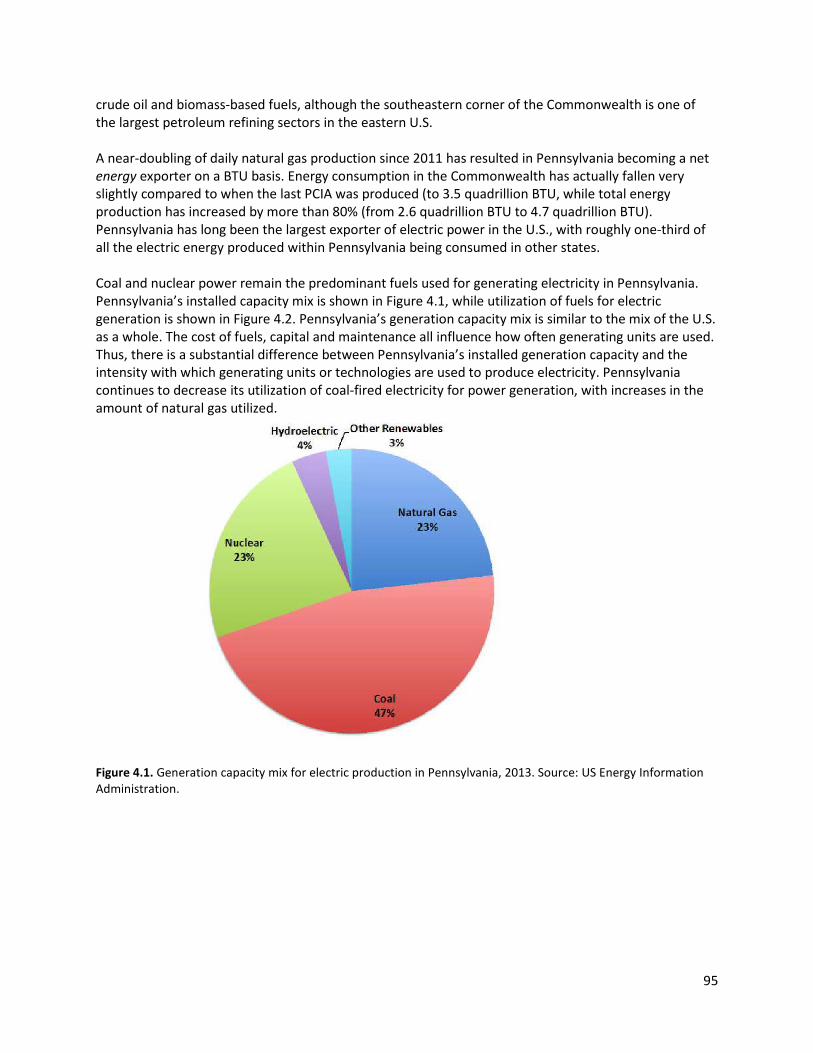
95

crude oil and biomass-based fuels, although the southeastern corner of the Commonwealth is one of the largest petroleum refining sectors in the eastern U.S. A near-doubling of daily natural gas production since 2011 has resulted in Pennsylvania becoming a net energy exporter on a BTU basis. Energy consumption in the Commonwealth has actually fallen very slightly compared to when the last PCIA was produced (to 3.5 quadrillion BTU, while total energy production has increased by more than 80% (from 2.6 quadrillion BTU to 4.7 quadrillion BTU). Pennsylvania has long been the largest exporter of electric power in the U.S., with roughly one-third of all the electric energy produced within Pennsylvania being consumed in other states. Coal and nuclear power remain the predominant fuels used for generating electricity in Pennsylvania. Pennsylvania’s installed capacity mix is shown in Figure 4.1, while utilization of fuels for electric generation is shown in Figure 4.2. Pennsylvania’s generation capacity mix is similar to the mix of the U.S. as a whole. The cost of fuels, capital and maintenance all influence how often generating units are used. Thus, there is a substantial difference between Pennsylvania’s installed generation capacity and the intensity with which generating units or technologies are used to produce electricity. Pennsylvania continues to decrease its utilization of coal-fired electricity for power generation, with increases in the amount of natural gas utilized.

Figure 4.1. Generation capacity mix for electric production in Pennsylvania, 2013. Source: US Energy Information Administration.

96

Figure 4.2. Fuel mix for electric production in Pennsylvania, 2013. Source: US Energy Information Administration. Prices for most energy commodities have continued to decline at the wholesale level in Pennsylvania. The most striking price declines have occurred in natural gas, where prices at Pennsylvania’s wholesale “trading hubs” have remained at levels well below the continental “Henry Hub” benchmark for most of 2014. These recent price trends for Pennsylvania trading hubs and the Henry Hub (a trading point in Louisiana that has long been the reference price for North American natural gas) are shown in Figure 4.3. The current and anticipated pace of Marcellus gas production is responsible for these pricing trends. Daily production has roughly doubled over the past two years, and Pennsylvania has seen the largest increase in proved natural gas reserves of any state in the U.S. In part due to regulatory structures for natural gas pricing, there is often a lag between a decline in wholesale prices for natural gas and changes in retail prices. While wholesale gas prices in Pennsylvania have been among the lowest in the U.S., citygate and retail prices have been 8 to 12 percent higher than the national average in Pennsylvania. The observed pricing trends are in part a reflection of an imbalance between supply and demand in the Marcellus producing area. Existing pipeline capacity is generally insufficient to move natural gas produced from the Pennsylvania Marcellus to other consumption regions during high-demand periods. The “stranded gas” that results depresses natural gas prices in Pennsylvania and increases prices in neighboring states. This has been most evident during the winter heating period, when wholesale natural gas prices in Maryland and Virginia rose to nearly forty times the level of prices in Pennsylvania. A number of pipeline projects are currently underway to increase Pennsylvania’s export capacity, although it is not clear whether the existing slate of projects will be sufficient to balance export capacity with Pennsylvania supply during high-demand periods.

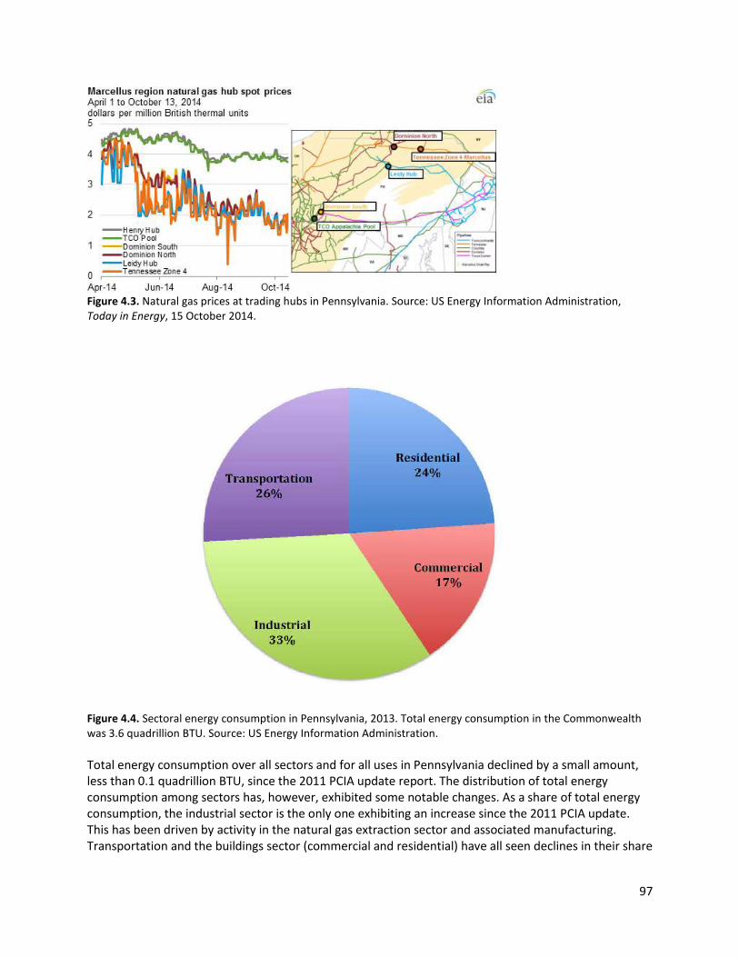
97

Figure 4.3. Natural gas prices at trading hubs in Pennsylvania. Source: US Energy Information Administration, Today in Energy, 15 October 2014.

Figure 4.4. Sectoral energy consumption in Pennsylvania, 2013. Total energy consumption in the Commonwealth was 3.6 quadrillion BTU. Source: US Energy Information Administration. Total energy consumption over all sectors and for all uses in Pennsylvania declined by a small amount, less than 0.1 quadrillion BTU, since the 2011 PCIA update report. The distribution of total energy consumption among sectors has, however, exhibited some notable changes. As a share of total energy consumption, the industrial sector is the only one exhibiting an increase since the 2011 PCIA update. This has been driven by activity in the natural gas extraction sector and associated manufacturing. Transportation and the buildings sector (commercial and residential) have all seen declines in their share

98

of total energy consumption. Figure 4.4 shows a breakdown of total energy consumption in Pennsylvania by sector. The industrial and transportation sectors consumed the largest amount of total energy, although industrial energy use declined by the largest amount.

4.3 Greenhouse-gas impacts of energy production and consumption in Pennsylvania The primary sources of energy-related greenhouse gas emissions in Pennsylvania continue to be associated with the electric power, transportation and industrial sectors. The burning of fossil fuels for space conditioning in homes or commercial buildings also contributes, but these effects are small by comparison, particularly since the majority of homes in Pennsylvania use natural gas for heating. Table 4.1 shows average and total carbon dioxide emissions from the burning of fossil fuels for various consumptive uses, including the generation of electricity. The increased use of natural gas for power generation in Pennsylvania, relative to coal and petroleum, has led to a decline in the greenhouse-gas footprint of Pennsylvania’s electric generation sector. It has likely also led to an increase in the greenhouse-gas footprint of Pennsylvania’s natural gas production sector, due to methane leakage across various portions of the production and delivery chain. While these leakages are difficult to quantify with precision, the Pennsylvania DEP has estimated 10 tons per year for the average drilling site in the Commonwealth in 2013 (PA DEP, 2015). Transportation-related emissions have also exhibited a decline since the 2011 PCIA update, in large part due to lower consumption figures for gasoline and diesel fuel reported by the U.S. Energy Information Administration. The figures for electricity generation are based on data specific to Pennsylvania, from the US Energy Information Administration and the Emissions and Generation Resource Integrated Database (eGRID) available through the US Environmental Protection Agency.5 The figures for home heating from fuel oil or natural gas are taken from Blumsack et al. (2009). The electric generation sector continues to be the largest source of greenhouse gas emissions in the Pennsylvania economy. As Table 4.1 demonstrates, Pennsylvania’s coal plants emit on average more than one ton of CO2 per megawatt-hour generated, while natural gas emits half as much CO2. The burning of refined petroleum for electricity is more carbon-intensive than burning coal, but oil-fired generation accounts for only a small portion of the Commonwealth’s electric-sector emissions.

5 http://www.epa.gov/cleanenergy/energy-resources/egrid/index.html.

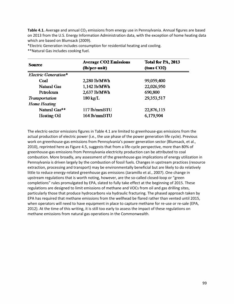
99

Table 4.1. Average and annual CO2 emissions from energy use in Pennsylvania. Annual figures are based on 2013 from the U.S. Energy Information Administration data, with the exception of home heating data which are based on Blumsack (2009). *Electric Generation includes consumption for residential heating and cooling. **Natural Gas includes cooking fuel.

The electric-sector emissions figures in Table 4.1 are limited to greenhouse-gas emissions from the actual production of electric power (i.e., the use phase of the power generation life cycle). Previous work on greenhouse-gas emissions from Pennsylvania’s power generation sector (Blumsack, et al., 2010), reprinted here as Figure 4.5, suggests that from a life-cycle perspective, more than 80% of greenhouse-gas emissions from Pennsylvania electricity production can be attributed to coal combustion. More broadly, any assessment of the greenhouse-gas implications of energy utilization in Pennsylvania is driven largely by the combustion of fossil fuels. Changes in upstream practices (resource extraction, processing and transport) may be environmentally beneficial but are likely to do relatively little to reduce energy-related greenhouse gas emissions (Jaramillo et al., 2007). One change in upstream regulations that is worth noting, however, are the so-called closed-loop or “green completions” rules promulgated by EPA, slated to fully take effect at the beginning of 2015. These regulations are designed to limit emissions of methane and VOCs from oil and gas drilling sites, particularly those that produce hydrocarbons via hydraulic fracturing. The phased approach taken by EPA has required that methane emissions from the wellhead be flared rather than vented until 2015, when operators will need to have equipment in place to capture methane for re-use or re-sale (EPA, 2012). At the time of this writing, it is still too early to assess the impact of these regulations on methane emissions from natural gas operations in the Commonwealth.

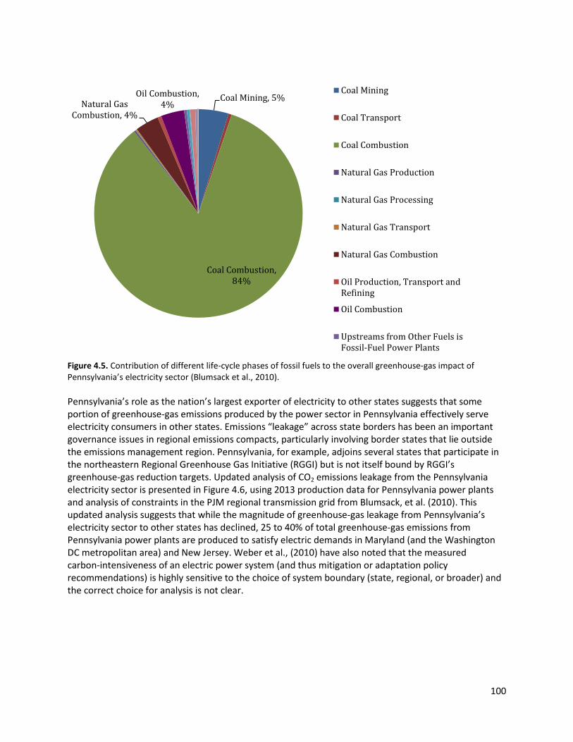
100

Figure 4.5. Contribution of different life-cycle phases of fossil fuels to the overall greenhouse-gas impact of Pennsylvania’s electricity sector (Blumsack et al., 2010). Pennsylvania’s role as the nation’s largest exporter of electricity to other states suggests that some portion of greenhouse-gas emissions produced by the power sector in Pennsylvania effectively serve electricity consumers in other states. Emissions “leakage” across state borders has been an important governance issues in regional emissions compacts, particularly involving border states that lie outside the emissions management region. Pennsylvania, for example, adjoins several states that participate in the northeastern Regional Greenhouse Gas Initiative (RGGI) but is not itself bound by RGGI’s greenhouse-gas reduction targets. Updated analysis of CO2 emissions leakage from the Pennsylvania electricity sector is presented in Figure 4.6, using 2013 production data for Pennsylvania power plants and analysis of constraints in the PJM regional transmission grid from Blumsack, et al. (2010). This updated analysis suggests that while the magnitude of greenhouse-gas leakage from Pennsylvania’s electricity sector to other states has declined, 25 to 40% of total greenhouse-gas emissions from Pennsylvania power plants are produced to satisfy electric demands in Maryland (and the Washington DC metropolitan area) and New Jersey. Weber et al., (2010) have also noted that the measured carbon-intensiveness of an electric power system (and thus mitigation or adaptation policy recommendations) is highly sensitive to the choice of system boundary (state, regional, or broader) and the correct choice for analysis is not clear.

Coal Mining, 5%

Coal Combustion, 84%

Natural Gas Combustion, 4%

Oil Combustion, 4%

Coal Mining

Coal Transport

Coal Combustion

Natural Gas Production

Natural Gas Processing

Natural Gas Transport

Natural Gas Combustion

Oil Production, Transport andRefining

Oil Combustion

Upstreams from Other Fuels isFossil-Fuel Power Plants

101

Figure 4.6. Estimated carbon dioxide exports from Pennsylvania, based on 2013 generation data and the analysis framework in Blumsack (2010). The figure is suggestive of how fossil-fired generation in Pennsylvania is utilized to satisfy electric demands in other states.

4.4 Climate change is likely to increase overall energy demand in Pennsylvania Analysis of Pennsylvania’s climate futures presented earlier in this report (Figure 2.23) suggests average temperature increases ranging from roughly 2 to 5 degrees Celsius by mid-century. Modeled temperature increases are generally smaller during the spring months of March, April and May. The models do not predict that mean temperatures will decline in any month in Pennsylvania by mid-century. The impacts of higher temperatures on Pennsylvania’s energy sector are likely to be most pronounced in the demand for electric power. Electricity is a commodity whose demand is driven largely by overall economic conditions and by weather conditions. Higher temperatures suggest an increase in air-conditioning demand and a decline in heating demand. Roughly 30% of Pennsylvania households currently use electricity for home heating, while there are few technological substitutes for electricity to supply cooling services (consumers could choose different cooling technologies, such as ceiling fans versus air conditioners, but all run on electric energy). The increase in electricity demand for cooling can thus be expected to be larger in magnitude than the decline in electricity demand for heating. The impacts of climate change in Pennsylvania on transportation and energy production are less certain. The overall demand for transportation is likely to be affected more by overall economic conditions (employment levels, disposable income) than by climate change per se. Mills and Andrey (2002) outline

102

aspects of climate change that are most likely to affect transportation systems. Some of these aspects would impact Pennsylvania’s transportation infrastructure positively and negatively. Extreme weather events can have negative impacts on air travel (as was observed during the “polar vortex” of 2013/14, which resulted in the cancellation of thousands of flights from the Philadelphia International Airport) and on shipping, though the economic consequences for Pennsylvania specifically have not been estimated. On the other hand, reductions in freeze-thaw cycles that may accompany a warming climate in Pennsylvania would suggest lower costs to maintain the Commonwealth’s highways, bridges and transportation infrastructure. Again, the economic benefits of these reduced costs have not been quantified. How climate change might impact production and harvesting of primary energy resources in Pennsylvania (which includes wind and solar harvesting as well as fossil fuels) is also uncertain. Relatively little research has been done on how climate change might impact the renewable energy industry, aside from the large body of work discussing renewable power generation resources as climate mitigation pathways. None of this research has focused on Pennsylvania specifically. Pryor and Barthelmie (2010) provide an assessment of how climate change might affect wind energy production, though their examples are focused on the European context. Overall, however, they suggest that impacts on overall wind resources are likely to be small, though the magnitude (higher or lower frequencies of wind speeds sufficient for power generation) are uncertain. Changes in wind resources may also be seasonal in nature (Sailor, Smith and Hart 2008). Specific to Pennsylvania’s wind industry, warmer temperatures could be expected to reduce the frequency of icing events, which would benefit the wind industry through higher levels of turbine availability during winter months. Modern oil and gas drilling rigs are designed to withstand extreme temperatures, well beyond heat extremes that climate assessments predict for Pennsylvania. Extreme cold conditions, such as those during the polar vortex of 2013/14, have been known to cause natural gas wells to freeze up and to cause disruptions in pipeline transportation of natural gas (PJM, 2014). Pennsylvania climate assessments for the mid-century period would suggest that these extreme cold-weather events would become less frequent. In this sense, climate change would not pose a threat to (and may contribute to the improvement of) reliability of energy production and delivery systems during cold-weather periods. Extreme weather events during warmer seasons may have very different impacts. Section 4.4 will address reliability issues in more detail. To address the implications of warming assessments for electricity demand in Pennsylvania, we have updated analysis originally performed for the 2009 PICA. We use hourly electricity demand for Pennsylvania from the PJM Interconnection, LLC for the period 2010 to the present to estimate a simple econometric model relating electricity demand to temperature. 6 Using 2013 demand as a base case combined with the warming assessments presented earlier in this report, we estimate changes in seasonal and annual electricity demand. The econometric model that we estimate is:

6 The geographic scope of PJM has grown since its inception as an Independent System Operator in 1998. Originally, portions of Pennsylvania lay outside the geographic footprint of PJM. We choose the period since 2010 to estimate our econometric model since nearly all of Pennsylvania was part of PJM by this time (and no part of Pennsylvania has since left PJM).

103

Electricityt = b0 + b1×HDDt + b2×CDDt + et, where Electricity represents hourly electricity demand in Pennsylvania, HDD measures heating degree days for a given hour (defined as the magnitude by which temperature during a given hour is below 65 degrees Fahrenheit) and CDD measures cooling degree days for a given hour (defined as the magnitude by which temperature during a given hour is higher than 70 degrees Fahrenheit), and et is the error term of the econometric equation. Heating and cooling degree days were calculated using an average temperature from weather stations at the Philadelphia and Pittsburgh International Airports. Figure 4.7 shows our estimates relating electricity demand in Pennsylvania to the warming assessments for the Commonwealth outlined in Section 2. This modeling exercise does not incorporate load growth due to population growth, but focuses only on that element of electricity demand influenced by the weather. The model also does not account for policies that will increase the market penetration of renewable generation, distributed generation, or peak load reduction such as Pennsylvania’s Alternative Energy Portfolio Standard (AEPS) or Act 129 beyond that which has actually been realized. For each season, we use the mean, 25th percentile, 75th percentile, minimum and maximum projected temperature changes, and we apply that temperature difference to hourly average temperatures for Pennsylvania for 2013. Changes in temperature (translated into changes into heating degree days and cooling degree days) were mapped into changes in overall electricity demand using the regression model described above. Each line in Figure 4.7 shows the percentage change in the distribution of hourly electricity demand throughout a year, relative to a “base case” of electricity demand in PJM in 2013. The figure suggests summer peaks in the PJM territory will become significantly more pronounced, and that increased cooling demand will more than offset decreases in electric heating demand. Changes in the total amount of electricity demanded during the course of a year, relative to the 2013 base case, are shown in Figure 4.8.

104

Figure 4.8. Increase in annual electricity demand in Pennsylvania for a range of warming projections.

Figure 4.7. Hourly percentage differences between Pennsylvania electricity demand for a range of warming projections, relative to a “base case” demand scenario based on 2013 data. Negative numbers indicate reductions in electric heating demand.

105

Electricity is generally the only energy source used for cooling, particularly at the residential level, though there are a variety of electricity-dependent technologies available, aside from electric compressors. The use of ice or deep-water thermal for cooling commercial spaces is beginning to gain in popularity, but even these systems depend on electricity to some degree (electricity is required to make the ice, for example). A variety of different fuels are used for space heating, the most common of which in Pennsylvania are natural gas, fuel oil and electricity. Space conditioning represents perhaps the most direct impact of climate change on energy use in Pennsylvania. The climate scenarios that make up the focus of this report all point towards an increase in the demand for cooling in the summer and a decline in the demand for heating in the winter; this is consistent with other impact assessments for Pennsylvania (Union of Concerned Scientists 2008, Shorr et al., 2009). We examine the net impact of climate change scenarios on the demand for heating and cooling using the model of space-conditioning demand for a Pennsylvania residence described in Blumsack, et al. (2009). We focus attention on this model due to its direct applicability to Pennsylvania’s climate. Figures 4.9 and 4.10 show the decline in heating demand and the increase in cooling demand for each of the six climate scenarios.

Figure 4.9. Proportional decline in household heating demand under six climate change scenarios, relative to a base case using 2007 temperatures. Only the top 6,200 hours are shown.

106

Figure 4.10. Proportional increase in household heating demand under six climate change scenarios, relative to a base case using 2013 temperatures. Only the top 2,500 hours are shown in the figure. Most economic research has focused on regulating greenhouse-gas emissions through price-based or market mechanisms, such as taxes on greenhouse gases or establishing a system of tradable permits for greenhouse-gas emissions. To date, Pennsylvania has not adopted these types of policies, though it acts as an “observing state” in the Regional Greenhouse Gas Initiative for trading of carbon dioxide credits in the northeastern US. Pennsylvania has adopted different types of policies that are relevant to the reduction of greenhouse gas emissions.

4.5 Climate Change and the Reliability of Energy Delivery Changes in average and extreme weather events associated with climate change can affect the reliability of energy delivery systems in two ways. First, extreme weather events such as hurricanes or ice storms can damage infrastructure. Recent examples affecting Pennsylvania over the past two years include superstorm Sandy in 2012 and the polar vortex winter weather event of 2013/14. The former of these extreme events damaged electricity delivery infrastructure, while the latter affected the ability of the natural gas pipeline system to respond to simultaneously high demands for heating of buildings and running of gas-fired power plants. Whether such extreme weather events (and what types) will become more common with a changing climate over multi-decadal time frames is uncertain. Second, increased cooling demand places higher demands on energy delivery infrastructure at times when these systems are already likely to be stressed. This stress alone may lead to equipment or component failures, particularly in electricity delivery systems. Electrical blackouts are a persistent problem, despite more than a decade of attention following the August 2003 northeastern blackout. There is no strong evidence that the frequency of large blackouts is decreasing (Hines, Talukdar and Apt,

107

2008), and the frequency of smaller blackouts may actually be increasing, for reasons that are not clear (Eto, et al, 2012). Small backup power generators have long been in use to allow electricity customers to continue to receive services when the power goes out. An increasingly economical alternative is “distributed generation,” which refers to small-scale power plants located at or near the end-use customer. Distributed generators can either serve a single customer or group of customers in an islanded operational mode, or they could be interconnected with one another or existing electric grids to operate in a “micro-grid” mode. Large, highly interconnected power grids such as those in North America allow utilities and customers to take advantage of economies of scale and inter-regional trade. This has both operational and economic advantages and can actually improve overall system reliability by providing more redundancy in the face of small-scale equipment failures. It does, however, leave all users on the system more vulnerable to large-scale blackouts. The distributed generation and micro-grid models may be economically advantageous to some type of users by allowing customers to avoid large peak-time demand charges for electricity provided by the grid (King and Morgan 2007; Siler-Evans, Morgan, and Azevedo 2012). A more distributed (rather than interconnected system) can be a more advantageous architecture when the risk of large-scale contingencies due to attacks or natural disasters becomes high (Zerriffi, Dowlatabadi and Farrell, 2007). The potential for distributed generation to provided needed electrical services in the face of natural disasters is clear, conditional upon fuel delivery infrastructures being operational in the aftermath of extreme weather events. Renewable generators such as small-scale wind turbines and solar panels are not dependent on infrastructure, so their performance will depend on resource availability. Gas-fired micro-turbines or combined heat and power (CHP) plants can continue to operate if natural gas pipelines are not interrupted for sustained periods of time. Because gas is effectively stored in pipelines at high pressures, the pipeline network can continue to deliver energy for a period of time after, say, a compressor station is rendered inoperable. It is worth noting, however, that the ability of customers to draw down linepack storage will depend on the type and location of the customer in question. Outages on the gas pipeline system do not, generally, affect all customers equally. In particular, there is some evidence that the polar vortex of 2013/14 impacted the ability of the natural gas system to deliver fuel reliably (PJM, 2014). In the face of climate-induced warming, distributed generation has two sources of value in helping to maintain electrical grid reliability. The first is that if blackouts do occur, distributed generation can substitute directly for grid-provided power. These benefits accrue largely to the owners and operators of distributed generation units, and will depend largely on the frequency of blackouts and the value that owners place on being able to continue to consume electricity. The second source of value is in helping to prevent blackouts from occurring in the first place. The experience of electric system operators with peak-time load curtailment programs has shown that reducing demand on the grid during lowers the risk of blackouts. Distributed generation could work in much the same way (indeed, many customers engaged in load-curtailment or electricity demand response programs shift from the grid to private generators when the curtailment call comes from the grid operator). This benefit accrues to all customers taking power from the grid and thus has some properties of a public good. Walawalkar, et al. (2008) have shown how these types of load curtailment programs can increase the efficiency of electric-grid operations, even when participants are given subsidies to take demand off the grid.

108

Using a framework developed by Govindarajan, et al. (2014), we provide some relatively simple estimates of the public-good value of distributed generation in preventing blackouts associated with rising temperatures (not extreme events, which are more difficult to model). The framework involves two steps. First, the likelihood of a blackout is modeled statistically as a function of electricity demand and temporal variables (like season of the year or time of day). Second, the duration of a blackout (conditional on one occurring) is modeled statistically as a function of these same types of variables – electricity demand, season and time of day that the blackout was instigated.7 We implemented the Govindarajan, et al. framework to focus on the likelihood of blackouts affecting Pennsylvania specifically, and to estimate the economic value of reducing blackout risk through increased use of distributed generation. We note that our analysis would also be relevant for increased energy conservation or peak-time electric load curtailment, since in our statistical approach the use of distributed generation is equivalent to simply removing demand from the grid. To estimate the economic value of blackout risk reduction, we use a method introduced by Sullivan (2010), which models blackout costs as a function of blackout size (number of customers or megawatts of demand interrupted) and duration. Because our statistical model is effectively based on past blackouts, it may be difficult to project the results of these models onto scenarios involving very large-scale adoption of distributed generation. We thus illustrate our results using a smaller-scale distributed generation scenario of up to 1,000 MW, which would represent at most a few percentage points of electrical demand in Pennsylvania. Figure 4.11 illustrates summer blackout risk reduction associated with two operational strategies for a building-integrated combined heat and power plant that operates in a manner to reduce peak-time electrical loads in the building (Following Electrical Load, or FEL) or in a manner to provide as much of the building’s thermal energy as possible (Following Thermal Load, or FTL). In the literature on combined heat and power operations, the FTL mode is generally considered to be more economically advantageous, but does not offer the same magnitude of reliability benefits as the FEL operational mode.

7 Large blackouts are required to be reported to the Department of Energy and the North American Electric Reliability Corporation (NERC), from whence the blackout data is drawn to conduct the econometric modeling. Electricity demand data is taken from the relevant system operator, in this case PJM.

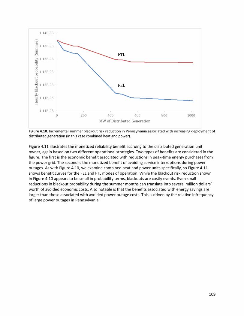
109

Figure 4.10. Incremental summer blackout risk reduction in Pennsylvania associated with increasing deployment of distributed generation (in this case combined heat and power). Figure 4.11 illustrates the monetized reliability benefit accruing to the distributed generation unit owner, again based on two different operational strategies. Two types of benefits are considered in the figure. The first is the economic benefit associated with reductions in peak-time energy purchases from the power grid. The second is the monetized benefit of avoiding service interruptions during power outages. As with Figure 4.10, we examine combined heat and power units specifically, so Figure 4.11 shows benefit curves for the FEL and FTL modes of operation. While the blackout risk reduction shown in Figure 4.10 appears to be small in probability terms, blackouts are costly events. Even small reductions in blackout probability during the summer months can translate into several million dollars’ worth of avoided economic costs. Also notable is that the benefits associated with energy savings are larger than those associated with avoided power outage costs. This is driven by the relative infrequency of large power outages in Pennsylvania.

1.11E-03

1.11E-03

1.12E-03

1.12E-03

1.13E-03

1.13E-03

1.14E-03

0 200 400 600 800 1000

Hou

rly

blac

kout

pro

babi

lity

(Sum

mer

)

MW of Distributed Generation

FTL FEL

110

Figure 4.11. Monetized owner benefits of distributed generation units in Pennsylvania. The left-hand axis shows the benefits to distributed generation owners in terms of avoided costs of power outages. The right-hand axis shows the benefits to distributed generation owners in terms of avoided peak-time energy purchases.

0

1

2

3

4

5

6

7

8

9

0

0.5

1

1.5

2

2.5

0 200 400 600 800 1000

Net

Ene

rgy

savi

ngs(

$ m

illio

n)

Ann

ual p

ower

out

age

cost

s ($

mill

ion)

Number of CHP units

Reliabilty benefitsFELReliability benefitsFTLEnergy savings FEL

Energy savings FTL

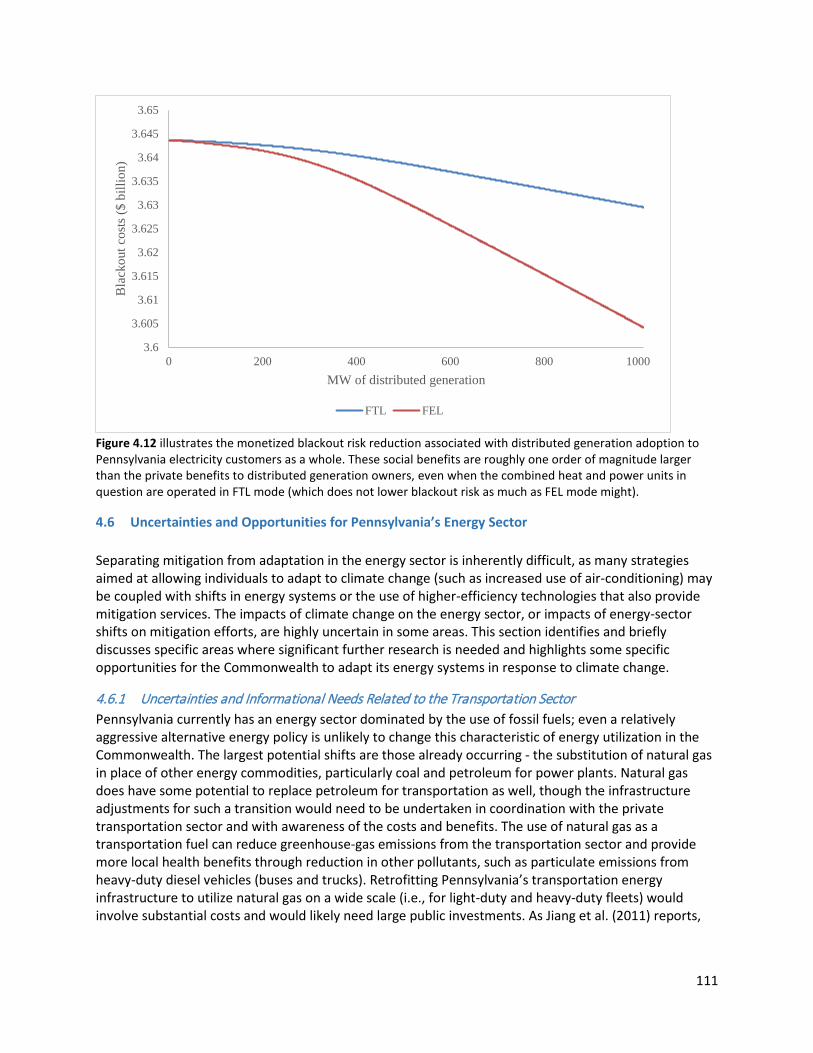
111

Figure 4.12 illustrates the monetized blackout risk reduction associated with distributed generation adoption to Pennsylvania electricity customers as a whole. These social benefits are roughly one order of magnitude larger than the private benefits to distributed generation owners, even when the combined heat and power units in question are operated in FTL mode (which does not lower blackout risk as much as FEL mode might).

4.6 Uncertainties and Opportunities for Pennsylvania’s Energy Sector Separating mitigation from adaptation in the energy sector is inherently difficult, as many strategies aimed at allowing individuals to adapt to climate change (such as increased use of air-conditioning) may be coupled with shifts in energy systems or the use of higher-efficiency technologies that also provide mitigation services. The impacts of climate change on the energy sector, or impacts of energy-sector shifts on mitigation efforts, are highly uncertain in some areas. This section identifies and briefly discusses specific areas where significant further research is needed and highlights some specific opportunities for the Commonwealth to adapt its energy systems in response to climate change.

4.6.1 Uncertainties and Informational Needs Related to the Transportation Sector Pennsylvania currently has an energy sector dominated by the use of fossil fuels; even a relatively aggressive alternative energy policy is unlikely to change this characteristic of energy utilization in the Commonwealth. The largest potential shifts are those already occurring - the substitution of natural gas in place of other energy commodities, particularly coal and petroleum for power plants. Natural gas does have some potential to replace petroleum for transportation as well, though the infrastructure adjustments for such a transition would need to be undertaken in coordination with the private transportation sector and with awareness of the costs and benefits. The use of natural gas as a transportation fuel can reduce greenhouse-gas emissions from the transportation sector and provide more local health benefits through reduction in other pollutants, such as particulate emissions from heavy-duty diesel vehicles (buses and trucks). Retrofitting Pennsylvania’s transportation energy infrastructure to utilize natural gas on a wide scale (i.e., for light-duty and heavy-duty fleets) would involve substantial costs and would likely need large public investments. As Jiang et al. (2011) reports,

3.6

3.605

3.61

3.615

3.62

3.625

3.63

3.635

3.64

3.645

3.65

0 200 400 600 800 1000

Bla

ckou

t cos

ts ($

bill

ion)

MW of distributed generation

FTL FEL

112

natural gas transportation may be most socially beneficial if limited to fleets of buses and some trucks, although the greenhouse-gas reduction impacts would not be that large. Natural gas vehicles are not the only option to reduce greenhouse-gas emissions from the transportation sector. Electrified transportation can, with appropriate changes in the power generation fleet, reduce greenhouse-gas emissions. Falling prices for fuels used in electric power plants are improving the economic case for electric vehicles. The situation with electric vehicles is largely the same as when the 2011 PCIA update came out. Consumers have some options to choose electric vehicle transportation, but other than in some fleet circumstances adoption rates have been very low. A combination of declines in vehicle prices, improvements in battery energy storage technology and a system to manage vehicle charging acceptable to both drivers and electric utilities are all needed before wide-scale electrification of the light-duty vehicle fleet would be a feasible option. More fundamentally, the costs (and possible benefits) of climate change to Pennsylvania’s transportation infrastructure have not been systematically investigated and are thus highly uncertain. Pennsylvania acts as a major hub for both shipping (by truck) and air travel. Both could be negatively affected if extreme weather events become more common with climate change. On the other hand, a warmer climate in Pennsylvania would have some positive impacts on the cost of maintaining transportation infrastructure in the Commonwealth. Formulating a coherent transportation policy related to climate change will be difficult without such analysis in hand.

4.6.2 Uncertainties related to coupled energy and water systems Electric power generation continues to represent the largest use of surface water in Pennsylvania, primarily in steam turbines for cooling. While not all of this water use is consumptive, Pennsylvania’s electricity infrastructure is dependent on reliable water supplies, particularly along the Commonwealth’s major rivers. The climate assessments presented in Section 2 do not suggest that Pennsylvania faces high risk of drought because of climate change. The opposite conclusion may indeed be drawn, that Pennsylvania will, on average, become wetter. Modeled drought conditions are most likely in the fall, a season when electricity demand in Pennsylvania is generally low. While climate change does not have the same drought implications for Pennsylvania as for southwestern areas, the models do suggest a higher drought probability for the month of September, relative to other times of the year. Particularly as Pennsylvania becomes warmer, electricity demand in September could become more similar to the levels that have historically been observed in the warmer months of July and August. Whether streamflow-induced plant curtailments could occur at Pennsylvania’s major generating facilities during these late-summer periods, and how often, represents a strong need for further research. Water-related curtailments are generally not considered in power system planning in the Mid-Atlantic region; this was the case when the 2011 PCIA update was completed as well. It continues to be unclear how or whether incorporating hydrologic constraints (or climate-induced uncertainty in the hydrologic cycle) would lead to different system planning decisions than those currently made.

4.7 Conclusions Broadly, the likely impacts of climate change on energy production and utilization in Pennsylvania have not changed significantly from the 2011 PCIA. Warming in Pennsylvania is likely to increase the demand for electricity for cooling in the summertime, and can be expected to decrease demand for heating fuels

113

(in Pennsylvania, the primary fuels used for heating are natural gas, fuel oil and electricity). The increase in cooling demand is likely to outweigh the decline in heating demand, implying that electricity consumption is likely to increase as a result of climate change. Perhaps more notably, peak-time electricity demand is likely to increase. Particularly in light of a recent ruling that states, not the federal government through the Federal Energy Regulatory Commission, should determine appropriate electric rate structures for demand reduction, Pennsylvania has a good opportunity, with historically low natural gas prices and abundant supplies, to consider comprehensive policies to encourage efficient building-integrated sources of backup power.

References Blumsack, S., 2010. “Implications of Marcellus Shale Natural Gas Development for the Economics of

Combined Heat and Power in the Mid-Atlantic U.S.,” report for the Mid-Atlantic Clean Energy Application Center.

Blumsack, S., P. Jaramillo, W. M. Griffin and H.S. Matthews, 2009. “Life-Cycle Greenhouse Gas Emissions Inventory for Electricity Generation in Pennsylvania,” report to the Pennsylvania Department of Environmental Protection.

Govindarajan, A. and S. Blumsack, 2014. “The Private and Social Value of Blackout Risk Reduction,” working paper.

Energy Information Administration, 2014. “State Energy Profiles,” http://www.eia.gov/state, last viewed on April 29, 2015.

Eto, J., LaCommare, K., P. Larsen, A. Todd and E. Fisher, 2012. “An Examination of Temporal Trends in Electricity Reliability Based on Reports from U.S. Electric Utilities,” Berkeley National Laboratory report, available at http://eetd.lbl.gov/publications/view/50191.

Fthenakis, V. and H. Kim. 2006. “Greenhouse-gas Emissions from Solar Electric- and Nuclear Power: A Life-Cycle Study,” Energy Policy 35, pp. 2549 – 2557.

Hines, P., S. Talukdar and J. Apt, 2008. “Large Blackouts in North America: Historical Trends and Policy Implications,” Energy Policy 37:12, pp. 5249-5259.

Jaramillo, P.; W. M. Griffin, and H. S. Matthews, 2007. “Comparative Life Cycle Air Emissions of Coal, Domestic Natural Gas, LNG, and SNG for Electricity Generation.” Environmental Science & Technology 41:17, pp.6290-6296.

Jiang, M., W.M. Griffin, C. Henrickson, P. Jaramillo, J. van Briesen and A. Venkatesh, 2011. “Life Cycle Greenhouse Gas Emissions of Marcellus Shale Gas,” Environmental Research Letters 6 034014.

King, Douglas E., and M. Granger Morgan, 2007. Customer-Focused Assessment of Electric Power Micro grids. Journal of Energy Engineering 133 (3) (September): 150–164. doi:10.1061/(ASCE)0733-9402(2007)133:3(150).

Mills, B. and J. Andrey, 2002. “Climate Change and Transportation: Potential Interactions and Impacts,” in The Potential Impacts of Climate Change on Transportation, U.S. Department of Transportation Workshop. Available online at http://2climate.dot.gov/documents/workshop1002/workshop.pdf.

Pennsylvania Department of Environmental Protection, 2015. “Air Emissions Data from Natural Gas Operations,” available at http://www.portal.state.pa.us/portal/server.pt/community/Emission%20Inventory/21810/Marcellus%20Inventory/1829967, last viewed on April 29, 2015.

PJM Interconnect, LLC. “Analysis of Operational Events and Weather Impacts During the January 2014 Cold Weather Events.”

Pryor, S. and R. Barthelmie, 2010. “Climate Change Impacts on Wind Energy: A Review,” Renewable and Sustainable Energy Reviews 14:1, pp. 430-437.

114

Sailor, D., M. Smith and M. Hart, 2008. “Climate Change Impacts for Wind Resources in the Northwest United States,” Renewable Energy 33:11, pp. 2393-2406.

Schorr, N., R. Najjar, A. Amato and S. Graham, 2009. “Household Heating and Cooling Energy Use in the Northeast USA: Comparing the Effect of Climate Change with those of Purposeful Behaviors,” Climate Research 39:1, pp. 19-30.

Siler-Evans, Kyle, M. Granger Morgan, and Inês Lima Azevedo, 2012. Distributed Cogeneration for Commercial Buildings: Can We Make the Economics Work? Energy Policy 42 (March): 580–590. doi:10.1016/j.enpol.2011.12.028.

Union of Concerned Scientists, 2008. “Climate Change in Pennsylvania: Impacts and Solutions for the Keystone State,” available online at http://www.ucsusa.org/global_warming/science_and_impacts/impacts/climate-change-pa.html#.VVEHUJNxpdc. Last viewed on April 29, 2015.

U.S. Environmental Protection Agency, 2012. “Summary of Requirements for Processes and Equipment at Natural Gas Well Sites,” available online at http://www.epa.gov/airquality/oilandgas/pdfs/20120417summarywellsites.pdf.

Walawalkar, R., S. Blumsack, J. Apt and S. Fernands, 2008. “An Economic Welfare Analysis of Demand Response in the PJM Electricity Market,” Energy Policy 36:10, pp. 3692-3702.

Zerriffi, Hisham, Hadi Dowlatabadi, and Alex Farrell, 2007. Incorporating Stress in Electric Power Systems Reliability Models. Energy Policy 35 (1) (January): 61–75. doi:10.1016/j.enpol.2005.10.007.

5 Forest Resources

5.1 Introduction The eastern hardwood forests of North America are resilient ecosystems. Pennsylvania’s forests have endured massive disturbances over the past two centuries, including their near-complete harvest during the late 19th and early 20th centuries (Whitney, 1990; Brose, Shuler, Van Lear & Berst, 2001). During this period millions of acres also burned as sparks and hot cinders from the coal-fired locomotives passing through cut-over areas ignited the slash left from the harvest. Exotic pests and diseases, including the chestnut blight, the gypsy moth, Dutch elm disease, the hemlock woolly adelgid, beech bark disease, and now the emerald ash borer, have or will soon also dramatically change Pennsylvania’s forests (Liebhold, MacDonald, Bergdahl & Mastro, 1995; Gottschalk, 2007). In addition, non-native plants, including trees such as ailanthus and Norway maple, shrubs such as bush honeysuckle, multiflora rose, Japanese knotweed, and privet, and herbaceous plants like Japanese stiltgrass and mile-a-minute weed, are invading the state’s forests (Webster, Jenkins & Jose 2006; Pennsylvania Department of Conservation and Natural Resources (DCNR), 2014). Overabundant deer populations have impaired the regeneration of tree species that they prefer to browse (Pedersen & Wallis, 2004; Latham et al., 2005; McShea, 2012) and accelerated the spread of invasive species (Knight et al., 2009). Unsustainable harvest practices such as high-grading and diameter-limit cutting have also taken their toll (Nyland, 1992). Finally, the soil chemistry of the state’s forest soils is being altered by atmospheric deposition (Horsley, Long, Bailey, Hallett, & Hall, 2000, 2008; Driscoll et al. 2001; Fenn et al. 2006). In spite of these assaults, Pennsylvania’s forests remain remarkably diverse and productive today. Climate change represents one additional stressor on Pennsylvania’s forests. Climate change is already radically affecting some forests around the world and, to a lesser degree, the forests of Pennsylvania. Climate change will likely continue to affect them in increasingly dramatic ways in the future. This chapter assesses the current state of our understanding of how Pennsylvania’s forests are likely to be

115

affected by climate change. It builds on similar chapters from two previous reports (McDill 2009, 2013) and focuses on new research that has been done since those reports or research that they did not cover. The most important results from those reports are sometimes repeated in less detail in order to keep this chapter somewhat self-contained. None of the new research reviewed here substantially changes the key findings of the previous reports. Key previous findings are:

1. Suitable habitat for plant and wildlife species is expected to shift to higher latitudes and elevations. This will reduce the amount of suitable habitat in Pennsylvania for species that are at the southern extent of their range in Pennsylvania or that are found primarily at high latitudes; the amount of habitat in the state that is suitable for species that are at the northern extent of their range in Pennsylvania will increase.

2. The warming climate will cause species inhabiting decreasingly suitable habitat to become stressed. Tree mortality rates are expected to increase and regeneration success is expected to decline for these species, resulting in declining importance of those species in the state.

3. Longer growing seasons, warmer temperatures, higher rainfall, nitrogen deposition, and increased atmospheric CO2 may increase overall forest growth rates in the state, but the increased growth rates for some species may be offset by increased mortality for others (see conclusion 2 above).

4. The state’s forest products industry will need to adjust to a changing forest resource. The industry could benefit from planting faster-growing species and from salvaging dying stands of trees. Substantial investments in artificial regeneration may be needed if large areas of forests begin to die back due to climate-related stress.

5. As with plants, some wildlife species will benefit from climate change and others will be negatively affected. A significant concern for wildlife is mis-timing of key events, such as broods hatching later or earlier than times of peak food supply.

6. Forests can contribute to the mitigation of climate change by sequestering carbon. It would be difficult to substantially increase the growth rates of Pennsylvania hardwoods, so the best opportunities most likely lie in preventing forest loss.

7. Forests can also be a significant source of biomass to replace fossil fuels. With regard to point 2 above, it should be noted that current forest inventory data do not show significant increases in tree mortality due to climate change. It is, nevertheless, still considered likely that such mortality will be observed in the future as the climate continues to change and climate envelopes shift further northward.

5.2 Projected climate change impacts Climate change is expected to affect Pennsylvania’s forests in a number of ways. The most dramatic effects are likely to be due to northward shifts in the regions of suitable habitat (habitat envelopes) for various tree species. Trees that were within their habitat envelope when they were established, especially those that are established at the southern extent of that envelop, may no longer be within that envelope decades later when they are mature. This will likely increase the stress on these individuals, potentially leading to directly to higher mortality rates or making them more susceptible to mortality from other causes, including, among other things, diseases, pests, and air pollution. On the other hand, climate change could lead to higher growth rates for some trees, through longer growing seasons, warmer temperatures, higher rainfall, greater nitrogen deposition, and a phenomenon termed

116

“CO2 fertilization.” A warming and wetter climate will also increase the metabolic rates of insect pests and allow them to spread further north. While there is broad scientific consensus about the general nature of the projected effects of climate change on eastern North American forests, there is nevertheless considerable uncertainty (Lindner et al. 2014) beginning with uncertainty about future emissions scenarios, which science cannot predict. In addition, the predictions of global circulation models (GCMs) vary among models and among runs of individual models. The process of downscaling output from GCMs using Regional Climate Models (RCMs) introduces additional uncertainty. Finally, forest sector models contribute even more uncertainty (Lindner et al. 2014). This combination of modeling efforts does, however, represent the scientific community’s best current understanding of how climate change is likely to affect our forest resources in the coming century. Furthermore, a number of effects have already been observed, and these observed effects are generally consistent with the predictions of the models. This combination of modeling projections and empirical validation provides some confidence in our general understanding of potential climate impacts. However, complex systems such as the earth’s climate and forested ecosystems do not always follow linear trends. It is possible – even likely – that thresholds exist that, when crossed, can lead to rapid and unexpected changes (Anderson, Carstensen, Hernández-García & Duarte 2009; Fagre et al. 2009).

5.2.1 Tree species distributions In general, the habitat envelopes for tree species are expected to move northward in the northern hemisphere and southward in the southern hemisphere, and to higher elevations globally (McKenney Pedlar, Lawrence, Campbell & Hutchinson, 2007; Iverson, Prasad and Matthews, 2008a; Mohan et al., 2009; McKenney, Pedlar, Rood & Price, 2011). The specific nature of these shifts will likely vary from one species to another (Higgins & Harte, 2006; Pucko, Beckage, Perkins & Keeton, 2011). Iverson et al. (2008a) and Iverson, Prasad, Matthews and Peters (2008b) used the Forest Service’s extensive Forest Inventory and Analysis (FIA) database to develop models that project shifts in the suitable habitat for 134 tree species in eastern North America under different climate change scenarios. McDill (2009) summarized their work and classified 35 of the tree species into six categories based on their projected response to the changing climate of the state: 1) species most at risk of being extirpated from the state, 2) species most likely to decline substantially in importance in the state, 3) species most likely to decline moderately in importance in the state, 4) species that are projected to either increase or decrease marginally, 5) species that are currently relatively common in the state and are most likely to increase in importance in the state, 6) species that are currently not common in the state and are most likely to increase in importance in the state (Table 5.1). The results in Table 5.1 are still the most current projections of tree species habitat suitability for Pennsylvania, and they are generally consistent with the silvics of the various species. Species that are at the southern extent of their range in Pennsylvania tend to be the most vulnerable, and species that are at the northern extent of their range in Pennsylvania are expected to thrive under climate change and increase in importance within the state. Note that some species – such as flowering dogwood, American beech, American elm, eastern hemlock and white ash – are declining or have already declined dramatically, but this is due to invasive pests and diseases, and not directly attributable to climate change. It is noteworthy that the species that are currently increasing most rapidly in importance – sweet birch and red maple (McWilliams et al., 2007) – are both in the category that is projected to decline moderately as climate change progresses. Uncertainty in the projections shown in Table 5.1 stem from many sources, including uncertainty about future emissions scenarios, from the GCMs used

117

to build the future climate scenarios, and from the models used to project how species habitat envelopes will shift in response to projected climate change. While there is considerable evidence from around the world that the suitable habitat envelopes of tree species are already shifting in response to climate change (c.f., Peñuelas & Boada, 2003; Jump, Hunt & Peñuelas, 2006; Lenoir et al., 2008; Bertin, 2008; Kelly & Goulden, 2008; Landhausser, Deshaies & Lieffers, 2010; Chen, Hill, Ohlemüller, Roy & Thomas, 2011; Delzon et al. 2013; Urli et al., 2014), evidence of such shifts in eastern North America is less abundant and more subtle. Examples from this region include Beckage et al. (2008) and Pucko, Beckage, Perkins & Keeton (2011), who observed an upslope shift in the northern hardwood–boreal forest ecotone in the Green Mountains of Vermont between 1962 and 2005, and Woodall et al. (2009), who observed that seedling densities of northeastern tree species were higher in the northern parts of their ranges than in the southern parts of their ranges, suggesting that tree migration in response to climate change is occurring through better regeneration success at the northern end of the species’ ranges. More recently, Potter & Woodall (2012) assessed 5-year patterns of change in the phylogenetic diversity of trees on 7,000 FIA plots in the eastern United States (US) and found shifts in biodiversity that are consistent with those expected under climate change. These include 1) greater change in seedling diversity than in tree diversity, 2) greater change in seedling diversity at higher latitudes and elevations, and 3) greater change in seedling diversity among species with higher dispersal capacity (Potter & Woodall 2012). An important question is whether natural migration of tree species will be able to keep up with shifts in their suitable habitat. If shifts in suitable habitat increase mortality along the southern boundaries of species’ ranges and if northern expansion fails to occur, then species ranges would contract. Zhu, Woodall, & Clark (2012) measured observed range shifts for 92 tree species in the eastern US and found that the ranges of 58.7% of the species were contracting. Only 20.7% of the species exhibited a northward range shift, and the ranges of 16.3% of the species appeared to be shifting southward. Thus, it does not appear that tree species are able to migrate effectively as their suitable habitat shifts, and that the primary response to shifting habitat envelopes is range contraction. Thus, active human intervention may be necessary to mitigate range contraction of most tree species. The study also suggests that the responses of tree species to climate change may be more complex than simply a northward shifting of their range.

118

Table 5.1. Classification of tree species in Pennsylvania by projected vulnerability to climate change (From McDill (2009) based on data from Iverson et al. (2008b)). Scientific Name Common Name Category Betula papyrifera paper birch Species most at risk of being extirpated from

the state Populus tremuloides quaking aspen Populus grandidentata bigtooth aspen Betula alleghaniensis yellow birch Fagus grandifolia American beech Species most likely to decline substantially in

importance in the state Prunus serotina black cherry Acer pensylvanicum striped maple Tsuga Canadensis eastern hemlock Acer rubrum red maple Species most likely to decline moderately in

importance in the state Acer saccharum sugar maple Pinus strobus eastern white pine Betula lenta sweet birch Fraxinus Americana white ash Tilia Americana American basswood Quercus rubra northern red oak Species that are projected to either increase

or decrease marginally Quercus prinus chestnut oak Liriodendron tulipifera yellow-poplar Sassafras albidum sassafras Carya glabra pignut hickory Nyssa sylvatica blackgum Juglans nigra black walnut Quercus alba white oak Ulmus Americana American elm Cornus florida flowering dogwood Carya tomentosa mockernut hickory Species that are currently relatively common

in the state and are most likely to increase in importance in the state

Quercus velutina black oak Acer saccharinum silver maple Juniperus virginiana eastern redcedar Pinus taeda loblolly pine Species that are currently not common in the

state and are most likely to increase in importance in the state

Pinus echinata shortleaf pine Diospyros virginiana common persimmon Morus rubra red mulberry Carya texana black hickory Quercus marilandica blackjack oak Ulmus alata winged elm Quercus stellate post oak

5.2.2 Tree mortality Pennsylvania is projected to be warmer and wetter in the future under climate change (Chapter 2, this report). While the state is projected to be wetter, much of the additional rain is projected to fall in the winter, with smaller increases in the summer and fall. Warmer temperatures increase evapotranspiration rates, which could lead to drier soil moisture conditions in the summer and fall (Hayhoe et al., 2007). High temperatures combined with drought have been shown to cause high rates of tree mortality in other regions (Adams et al., 2009; van Mantegem et al., 2009; Allen et al., 2010;

119

Anderegg, Kane, & Anderegg, 2013). While these conditions could occur more frequently in Pennsylvania as a result of climate change, at present there is little evidence of increased tree mortality in eastern North America that can be attributed to climate change. In their analysis of causes of tree mortality in the eastern US, Dietze and Moorcroft (2011) found that air pollution and stand characteristics such as age and density are far more important factors driving tree mortality than climate. This could be because climate envelopes in Pennsylvania have not shifted substantially at present and because mature trees are less sensitive to climate extremes than younger trees and tree regeneration. Thus, climate impacts are more likely to be observed first in tree regeneration rates, rather than in mortality rates of mature trees. There has been some speculation in the literature (e.g., Hänninen 2006) that trees will experience greater frost damage, and hence mortality, as leaves tend to unfold earlier in the year when the risk of frost is still high. However, there is little empirical evidence to support this hypothesis, and the results of at least one recent modeling study (Morin & Chuine 2014) contradict the hypothesis. Weather extremes, including both high and low temperatures, have been increasing in recent decades (Rummukainen, 2012). Huntington et al. (2009) derived an index of potential hurricane destructiveness and found that it has been increasing over the past 30 years. Increasing storm severity could lead to increased tree mortality, but our understanding of the impact of climate on the frequency and severity of storms is highly uncertain at present (Rummukainen, 2012).

5.2.3 Forest growth rates Climate change should increase average tree growth rates in Pennsylvania due to higher atmospheric CO2 concentrations, longer growing seasons, and increased precipitation. Nitrogen (N) deposition could also play a role in increasing growth rates. Free air CO2 enrichment (FACE) experiments have consistently shown substantial positive growth responses to CO2 concentrations in the atmosphere (Norby et al., 2005). However, potential growth increases from increased atmospheric CO2 concentrations are often constrained by other factors, including soil fertility – particularly N limitations – and water availability (Finzi et al., 2006; Johnson, 2006; Norby et al., 2010), so the size of the increase in productivity is difficult to predict. The warming of the climate is also expected to increase plant growth (Gunderson et al., 2012), primarily because of the longer growing season. In the eastern US, where water availability and soil nutrients are less likely to constrain forest growth, and where N deposition is relatively high, climate change will most likely lead to increased average forest growth rates (Luo et al., 2008; Campbell et al. 2008). For example, in one study of upland oak forests in Tennessee, carbon storage rates were projected to increase by 20% by 2100 (Hanson et al., 2005). If warmer temperatures lead to drier soil moisture conditions, growth could be reduced, however. Growth increases could also be offset by increased mortality rates due to species that are no longer well adapted to the climate where they are located or due to increased insect and disease outbreaks.

5.2.4 Plant diseases and insect pests Even without climate change, a variety of insect pests, including the elm spanworm, the emerald ash borer, the gypsy moth, the hemlock woolly adelgid, and the two-lined chestnut borer, have caused substantial mortality in Pennsylvania’s forests (Dukes et al., 2009). Rising temperatures increase insect metabolic and reproductive rates (Gillooly et al., 2002; Clark & Fraser, 2004; Robinet & Roques 2010), so climate change could make outbreaks of these pests more destructive and harder to control. Furthermore, insect ranges are often limited by minimum winter temperatures, so as the climate warms they, like other organisms, are able to migrate further northward and to higher elevations (Logan et al., 2003; Robinet & Roques 2010). The northern limit of the hemlock woolly adelgid is currently believed to be determined by minimum winter temperatures, and it has been able to spread to the north and east

120

in recent years due to warmer winters (Dukes et al., 2009, Fitzpatrick et al., 2012). Southern pines are not currently common in Pennsylvania, but in the future they could become increasingly important in the state as the climate warms (Table 5.1). However, the warming climate may also allow the southern pine beetle, which can cause devastating mortality in southern pine stands, to spread into the state as well (Tran et al., 2007). As with insects, climate can influence the life histories and ranges of plant diseases. For example, the virulence of sudden oak death outbreaks has been increased by climate change (Sturrock et al. 2011), and Swiss needle cast outbreaks are enhanced by warm winters and wet springs (Stone et al. 2008). Both of these diseases are found in Pennsylvania, but mainly on urban trees. Pennsylvania’s forests are affected by a variety of tree pathogens, such as armillaria root rot, elm yellows, beech bark disease, chestnut blight, dogwood anthracnose, Dutch elm disease, and oak wilt, among others (Dukes et al., 2009). Because of their diversity, general conclusions about how they will fare under climate change are not possible. It is, however, likely that some of these pathogens will benefit from climate change and others will not. Climate change can also increase the vulnerability of trees to pests and pathogens if they are stressed by drought or high temperatures (Sturrock et al. 2011; Vose, Peterson, & Patel-Weynand, 2012).

5.2.5 Wildlife In general, as with plants, wildlife species’ ranges have been observed to be and are projected to continue to move northward and to higher elevations (Parmesan & Yohe 2003). Species at the southern extent of their range in Pennsylvania, such as the marten (Martes americana) (Carroll, 2007) and Canada lynx (Lynx canadensis) will likely decline. The Canada lynx, which is already rare in Pennsylvania, will likely be extirpated from the state (Hone, et al., 2011; Yan et al., 2013). Bobcats (Lynx rufus), on the other hand, will likely expand their ranges to the north. Range shifts in animals are driven by both direct effects – shifts in the region where climatic factors are optimal – and indirect effects, such as shifts in the range of the plant communities that provide key habitat conditions or shifts in the range of key prey species (Matthews et al., 2011). Since it is not likely that all of these factors will shift equally, it is also likely that species will have to adapt to changing conditions. Matthews et al. (2011) developed statistical models to project the climate suitability for 39 tree species under a range of climate scenarios and then used a combination of climate projections and tree range projections to project the regions of habitat suitability for 147 bird species. Results varied with different climate models and emissions scenarios, but they projected declining ranges for 61-79 bird species and increasing ranges for 38-52 species. In addition to range shifts, the timing of key life-cycle events is changing for both plants and animals. Birds are one of the most-studied wildlife taxa, and migratory birds are arriving and breeding earlier in the spring (Marra et al., 2005; Vitale & Schlesinger, 2011) and migrating later in autumn (Schummer et al., 2010; Notaro et al., 2014). Studies in Europe of tits (Paridae) and flycatchers (Muscicapidae) have found (Visser et al., 1998; Both 2010) found that earlier breeding resulted in lower breeding success because it resulted in mis-timing of brooding with peak prey abundance. However, in a study of the North American Black-Throated Blue Warbler, Townsend et al. (2013) found that early breeding increased the incidence of double-brooding and led to higher overall fecundity. Changing climatic conditions outside of Pennsylvania can also impact the demographics of migratory bird species. For example, changes in tropical overwintering areas (Central and South America, the Caribbean) can influence the populations of neotropical migrants that breed in Pennsylvania. Wilson et al. (2011) observed that American redstart (Setophaga ruticilla) populations responded to climate in the Caribbean, where they overwinter, which is in turn influenced by variation in the El Niño Southern

121

Oscillation (ENSO). Sillet et al. (2000) found similar results for Black-Throated Blue Warblers (Dendroica caerulescens), and Mazzerole et al. (2005) observed similar responses in the populations of Yellow Warblers (Dendroica petechia) in Manitoba. Paxton et al. (2014) also found that migratory birds that overwinter in South America were negatively affected during El Niño years, but they did not observe significant effects for birds that overwinter in Central America and the Caribbean. Bats provide another example of the complex ways climate change can potentially impact wildlife species. Populations of hibernating bat species in the northeastern U.S. have already been substantially reduced as a result of White-Nose Syndrome. It is hard to say whether climate change will exacerbate these losses or ameliorate them (Frick et al. 2010). On the one hand, bats could benefit from shorter winters through reduced hibernation times and lower stored energy requirements, and longer foraging seasons provide more time for building up fat stores for hibernation. On the other hand, warmer winters could result in more frequent periods of arousal, increasing energy requirements for hibernation. Furthermore, drier summers could result in fewer insects for insectivorous bats to feed on.

5.3 Mitigation and adaptation Climate change is already occurring and will continue to occur, albeit at different rates, under all emissions scenarios. However, forest carbon management can lessen the amount of change that will occur. Furthermore, because climate change is also inevitable, forests must also be managed to increase their resiliency in the face of climate change.

5.3.1 Forest management for climate change mitigation Forests represent one of the significant pools of terrestrial carbon (Jandl et al., 2007). The size of this pool can be increased through forest management, primarily by increasing stand densities, increasing rotation lengths, and reducing mortality. Furthermore, removal rates from this pool can be decreased by reducing conversion of forests to non-forest land uses. Nearly three quarters of Pennsylvania’s 16.6 million acres of forestland are privately owned (McWilliams et al., 2007). Private forests in Pennsylvania are managed for a wide range of objectives, and carbon storage seldom ranks high among them (Butler & Leatherberry, 2004). Policy-makers’ ability to influence the management of these privately-owned lands is also currently limited, but education and incentives can make some difference without being overly heavy-handed. New mechanisms to increase incentives for carbon sequestration on private lands, such as carbon banking and trading, are being developed, but are currently in their infancy and many issues remain regarding how they should be designed to maximize their efficacy (Galik and Cooley, 2012). While Pennsylvania’s public forests make up only 29% of the forest land in the state, this is still a fairly substantial amount of land, representing a significant carbon pool. Even on public forests, however, carbon storage is only one of many management objectives (DCNR, 1992). Of all the options for increasing the pool of carbon stored in Pennsylvania’s forests, the greatest immediate impact will likely be achieved by reducing conversion of forestland to non-forest land uses. In the longer run, afforestation of economically marginal lands and restocking of poorly stocked forestland could also be effective ways to increase forest carbon storage in the state. In the long run, producing energy with wood rather than fossil fuels could also mitigate the buildup of greenhouse gasses in the atmosphere. So-called “low-use wood” is abundant in Pennsylvania and has relatively little value for alternative uses (Pennsylvania Hardwoods Development Council (PA HDC), 2008). However, while many consider woody biomass to be “carbon neutral,” the true picture is somewhat complicated. Harvesting more wood biomass for energy production inevitably leads, at least in the short run, to less carbon stored in forests and emission of this carbon to the atmosphere.

122

Furthermore, because the energy content per ton of carbon emitted in the burning of wood is less than with coal, and significantly less than with natural gas, replacing these fossil fuels with biomass energy will in the short run require emitting more carbon into the atmosphere per unit of energy produced. Assuming that the harvested wood is eventually replaced by new growth, this “carbon debt” will be offset over time by the regrowth of the forest, ultimately resulting in a net carbon benefit. But the time required to achieve a net reduction in atmospheric carbon by substituting woody biomass for fossil fuels ranges from a few years to more than a century (Manomet, 2010; McKechnie et al., 2011). The length of time needed to offset this carbon debt varies with 1) the efficiency of the process used to convert the wood to energy, 2) the type of fossil fuel technology that is replaced, 3) whether the wood used is from standing trees (that presumably would not have been harvested or died anyway) or whether it is from harvest residues (which would have eventually released their carbon through decomposition), and 4) the rate of regrowth of the harvested forest (McKechnie et al., 2011). According to Manomet (2010), which only considers the harvest of live trees, the length of time required to pay off this carbon debt ranges from 5 years when woody biomass from harvested trees (that wouldn’t have been harvested or died otherwise) is used to replace oil-fired thermal and CHP facilities to more than 90 years when natural gas electrical generation capacity is replaced. McKechnie et al. (2011) found that the time required to repay the carbon debt ranged from 16 to more than 100 years for a variety of scenarios. A more recent study (Sathre and Gustavsson, 2011) compared the climate impacts of combustion of forest residues (harvest slash and stumps) with combustion of coal and natural gas and found that climate effects (as measured by cumulative radiative forcing (CRF)) were detrimental (CRF was increased) for 10-25 years, but beneficial after that. Cumulatively, over the modeled 240-year time period, the climate impacts of substituting woody biomass for fossil fuels was significantly beneficial (Sathre and Gustavsson, 2011).

5.3.2 Adapting Pennsylvania’s forests for a changing climate As mentioned at the beginning of this chapter, Pennsylvania’s forests are resilient. Much of this resilience comes from the diversity of tree and plant species found in these forests. This diversity has been and is being negatively affected by a number of problems, including invasive insects and diseases, such as the chestnut blight, Dutch elm disease, elm yellows, the hemlock woolly adelgid, and the emerald ash borer. Efforts to address these problems and to maintain and restore the native diversity of Pennsylvania’s forests will make them healthier, more productive, and more resilient to climate change. Regeneration of diverse tree species is critical to maintaining healthy, resilient forests. Overabundant deer populations can impair the successful regeneration of diverse tree species (Latham et al., 2005). Thus, management of deer populations to allow for a diversity of tree regeneration can also increase the ability of the state’s forests to adapt successfully to a changing climate. Ecosystems have never been static entities and have always adapted to change. The challenge with climate change is the rate at which change is happening. “Climate velocity” estimates attempt to measure of how far plants and animals would have to shift their ranges each year to stay in their climate envelope (Loarie et al., 2009). Loarie et al.’s (2009) estimate of climate velocity (°C per km divided by °C per year) is 2.6 miles (4.2 km) per decade under the IPCC A1B emissions scenario. Using a different methodology and a different time period (1916 and 2005), Dobrowski et al. (2013) calculated climate velocity for minimum temperature (Tmin), actual evapotranspiration (AET), and deficit over the contiguous US and found average rates of only 0.50 miles (0.81 km), 0.61 miles (0.98 km), and 0.52 miles (0.84 km) per decade. Migration rates such as these are likely achievable for mobile species. For example, Chen et al. (2011) estimated that mobile populations of plants and animals have moved to higher latitudes at a median rate of 10.5 miles (16.9 km) per decade and to higher elevations at a median rate of 36 feet (0.011 km) per decade in response to recent climate changes. Iverson et al.

123

(2004) estimate that tree species can migrate at rates of up to 0.6 to 1.2 miles (1-2 km) per decade. However, habitat fragmentation may impede such migration rates. One possible solution, termed “assisted migration,” is to move species or genotypes to new locations that are further north or at higher elevations than where they are currently found (Appell, 2009; Hewitt et al., 2011). However, there is considerable uncertainty about how to do this in practice (Davidson & Simkanin, 2008). A more promising solution is to maintain and increase the connectivity of the state’s forests. Minimizing forest loss and fragmentation, combined with strategic restoration efforts to improve connectivity, is an important strategy for enhancing the resilience of the state’s forests under climate change.

5.4 Forest management opportunities related to climate change The primary forest management opportunities related to climate change are: 1) carbon trading, 2) increased markets for low-use wood for energy production, and 3) potentially renewed interest and will to manage forests for their long-term health and resiliency. Current options for Pennsylvania landowners to engage in carbon trading are limited. Currently the only active carbon registries for forestry projects in the US are the Climate Action Reserve (CAR), which is primarily active in California, and the Regional Greenhouse Gas Initiative (RGGI), which is active in Connecticut, Delaware, Maine, Maryland, Massachusetts, New Hampshire, New York, Rhode Island, and Vermont. Forest landowners in Pennsylvania can voluntarily participate in these programs, but they are unlikely to receive any monetary compensation for commitments to increase the carbon storage on their properties. This may change, however, if the political climate results in a more states joining these initiatives, or if a carbon cap and trade program is passed at the national level. Markets for wood energy were strong in 2008 when oil prices peaked at over $140 per barrel. Since then, however, oil and gas production in the US has boomed and energy prices have fallen dramatically. Thus, it is unlikely that the market for wood energy will grow significantly in the near future. This will likely only change if there is a substantial political commitment to decrease our use of fossil fuels. Even if this happens, solar energy costs continue to decline, and wood will have a hard time competing with solar energy for many applications. In the medium run, wood energy is likely to be used mainly for small-scale heating applications. However, if the potential of cellulosic biofuels is realized, cellulose-based ethanol and other advanced biofuels could potentially replace more than one third of the liquid fuels used in the US (Perlack et al., 2005; Zerbe, 2006; Bergman and Zerbe, 2008). In the coming decades, climate change will significantly alter the forest landscapes of Pennsylvania. The amount of change will challenge the ability of forest ecosystems to adapt through natural mechanisms. Humans will need to be more actively involved in the management of these ecosystems if we wish to have forests that provide the level of ecosystem services that we have come to expect from them. One can hope that this outcome will lead to a greater commitment by society to manage these resources to maintain their health and resiliency.

5.5 Forest management barriers related to climate change The primary barriers to managing Pennsylvania’s forests for health and resiliency in the face of climate change are: 1) lack of knowledge, 2) the large number of private forest landowners, 3) continued fragmentation of forest landscapes, and 4) the host of confounding, interrelated challenges to managing forests for diversity, health and resiliency.

124

Lack of knowledge regarding how forests will fare under a changed climate is a huge problem for forest managers. In the past, forest managers believed that they could learn from their experience and apply those lessons to future forests. However, with a rapidly changing climate, what worked in the past may not work in the future. Adaptive management, or learning as you go, will become increasingly important in the future. Pennsylvania’s private forests are owned by roughly half a million forest owners (Butler 2008). Influencing the management of this many ownerships is a daunting task; merely communicating with this many people is a challenge. Education and incentives have been tried and have had only a marginal effect on the management of these forests. Large enough incentives to make a difference would likely be very expensive. Heavy-handed regulation would be unpopular and likely politically unviable. A key challenge in the coming decades will be maintaining forest habitat connectivity in the more heavily forested parts of the Marcellus Shale region where natural gas development has resulted in expansion of existing roads, development of new roads, and development of pipeline corridors, all of which have contributed to further fragmentation of the landscape. Finally, if Pennsylvania’s forests are to remain resilient in the face of climate change, forest managers and policymakers must address all of the other major threats to their health and diversity. These include insect pests, diseases, invasive plants and animals, overabundant deer populations, unsustainable harvest practices, and atmospheric deposition. All of these problems are interrelated and must be addressed holistically with the goal of maintaining, restoring, and possibly creating healthy forest ecosystems. This is, of course, easier said than done.

References Adams, H.D., Guardiola-Claramonte, M., Barron-Gafford, G.A., Villegas, J.C., Breshears,D.D., Zou, C.B.,

Troch, P.A., Huxman, T.E., (2009). Temperature sensitivity of drought-induced tree mortality: implications for regional die-off under global-change-type drought. Proceedings of the National Academy of Sciences of the United States of America, 106, 7063–7066.

Allen, C. D., Macalady, A. K., Chenchouni, H., Bachelet, D., McDowell, N., Vennetier, M., Kitzberger, T., Rigling, A., Breshears, D. D., Hogg, E. H., et al. (2010). A global overview of drought and heat-induced tree mortality reveals emerging climate change risks for forests. Forest Ecology and Management, 259, 660–684.

Anderegg, W.R.L., Kane, J.M., & Anderegg, L.D.L. (2013). Consequences of widespread tree mortality triggered by drought and temperature stress. Nature Climate Change, 3, 30–36.

Anderson, T., Carstensen, J., Hernández-García, E., & Duarte, C.M. (2009). Ecological thresholds and regime shifts: approaches to identification. Trends in Ecology and Evolution, 24, 49–57.

Appell, D., 2009. Can ‘‘Assisted Migration’’ Save Species from Global Warming? Scientific American Magazine, March 2009.

Beckage , B., Osborne, B., Gavin, D.G., Pucko, C., Siccama, T., & Perkins, T. (2008). A rapid upward shift of a forest ecotone during 40 years of warming in the Green Mountains of Vermont. Proceedings of the National Academy of Sciences, 105(11), 4197-4202.

Bergman, R. & Zerbe, J. (2008). Primer on Wood Biomass for Energy. USDA Forest Service Forest Products Laboratory. Madison, Wisconsin. http://www.fpl.fs.fed.us/documnts/tmu/biomass_energy/primer_on_wood_biomass_for_energy.pdf

125

Bertin, R.I. (2008). Plant phenology and distribution in relation to recent climate change. Journal of the Torrey Botanical Society, 135, 126–146.

Both, C. (2010). Food availability, mistiming, and climatic change. In: Møller AP, Fielder W, Berthold P, editors. Effects of Climate Change on Birds. Oxford: Oxford University Press. 129–147.

Brose, P., Schuler, T. Van Lear, D., & Berst, J.( 2001). Bringing fire back: The changing regimes of the Appalachian mixed-oak forests. Journal of Forestry, 99(11), 30-35.

Butler, B.J. & Leatherberry, E.C. (2004). America’s family forest owners. Journal of Forestry 102(7), 4-9. Butler B.J. (2008). Family forest owners of the United States, 2006: A technical document supporting the

Forest Service 2010 RPA assessment. US For. Serv. Gen. Tech. Rep. NRS-27, North.Res. Stn., Newtown Square, PA. 72 p.

Campbell, J.L.; Rustad, L.E.; Boyer, E.W. [et al.]. (2009). Consequences of climate change for biogeochemical cycling in forests of northeastern North America. Canadian Journal of Forest Research, 39, 264–284.

Carroll, C. (2007). Interacting effects of climate change, landscape conversion, and harvest on carnivore populations at the range margin: marten and lynx in the northern Appalachians. Conservation Biology 21(4), 1092–1104.

Chen, I-C., Hill, J.K., Ohlemüller, R., Roy, D.B., & Thomas, C.D. (2011). Rapid range shifts of species associated with high levels of climate warming. Science, 333 (6045), 1024-1026.

Clark, A., & Fraser, K.P.P. (2004). Why does metabolism scale with temperature? Functional Ecology, 18, 243-251.

Davidson, I., and Simkanin, C. (2008). Skeptical of assisted colonization. Science 322, 1048–1049. Delzon, S., Urli, M., Samalens, J.-C., Lamy, J.-B., Lischke, H., Sin, F., Zimmermann, N.E., & Porté, A.J.

(2014). Field evidence of colonisation by Holm oak, at the northern margin of its distribution range, during the Anthropocene period. PLOS ONE, 8(11), e80443.

Dobrowski, S. Z., Abatzoglou, J., Swanson, A. K., Greenberg, J. A., Mynsberge, A. R., Holden, Z. A. and Schwartz, M. K. (2013), The climate velocity of the contiguous United States during the 20th century. Global Change Biology, 19, 241–251

Driscoll, C.T., Lawrence, G.B., Bulger, A.J., Butler, T.J., Cronan, C.S., Eagar, G., Lambert, K.F., Likens, G.E., Stoddard, J.L., & Weathers, K.C. (2001). Acidic deposition in the northeastern United States: Sources and inputs, ecosystem effects, and management strategies. BioScience, 51, 180–198.

Dukes, J.S., Pontius, J., Orwig, D., Garnas, J.R., Rodgers, V.L., Brazee, N., Cooke, B., Theoharides, K.A., Stange, E.E., Harrington, R., Ehrenfeld, J., Gurevitch, J., Lerdau, M., Stinson, K., Wick, R., & Ayres, M. (2009). Responses of insect pests, pathogens, and invasive plant species to climate change in the forests of northeastern North America: What can we predict? Canadian Journal of Forest Research, 39(2), 231-248.

Fagre, D.B.; Charles, C.W.; Allen, C.D. [et al.]. (2009). Thresholds of Climate Change in Ecosystems: Final Report, Synthesis, and Assessment Product 4.2. U.S. Climate Change Science Program and the Subcommittee on Global Change Research. Reston, VA: U.S. Department of the Interior, Geological Survey. 70 p.

Fenn, M.E., Huntington, T.G., McLaughlin, S. B. Eager, C., Gomez, A., & Cook, R.B.. (2006). Status of soil acidification in North America. Journal of Forest Science, 52, 3-13.

Finzi, A.C.; Moore, D.J.P.; DeLucia, E.H. [et al.]. (2006). Progressive nitrogen limitation of ecosystem processes under elevated CO2 in a warm-temperate forest. Ecology, 87: 15–25.

Fitzpatrick, M.C.; Preisser, E.L.; Porter, A. [et al.]. (2012). Modeling range dynamics in heterogeneous landscapes: invasion of the hemlock woolly adelgid in eastern North America. Ecological Applications. 22: 472–486.

Frick, W.F., Reynolds, D.S., & Kunz, T.H. (2010) Influence of climate and reproductive timing on demography of little brown myotis Myotis lucifugus. J. of Animal Ecol. 79, 128–136.

126

Galik, C.S., & Cooley, D.M. (2012). What makes carbon work? A sensitivity analysis of factors affecting forest offset viability. Forest Science, 58(5), 540-548.

Gillooly, J.F.; Charnov, E.L.; West, G.B. [et al.]. (2002). Effects of size and temperature on developmental time. Nature, 417, 70–73.

Gottschalk, K.W., ed. (2007). Proceedings, 18th U.S. Department of Agriculture Interagency Research Forum on Gypsy Moth and Other Invasive Species 2007; 2007 January 9-12; Annapolis, MD. Gen. Tech. Rep. NRS-P-28. Newtown Square, PA: U.S. Department of Agriculture, Forest Service, Northern Research Station, 84 p.

Gunderson, C.A.; Edwards, N.T.; Walker, A.V. [et al.]. (2012). Forest phenology and a warmer climate—growing season extension in relation to climatic provenance. Global Change Biology, 18, 2008–2025.

Hänninen, H. (2006). Climate warming and the risk of frost damage to boreal forest trees: identification of critical ecophysiological traits. Tree Physiol. 26: 889–898.

Hanson, P.J.; Wullschleger, S.D.; & Norby, R.J. (2005). Importance of changing CO2, temperature, precipitation, and ozone on carbon and water cycles of an upland-oak forest: incorporating experimental results into model simulations. Global Change Biology, 11, 1402–1423.

Hayhoe, K., Wake, C.P., Huntington, T.G., Luo, L., Schwartz, M.D., Sheffield, J., Wood, E., Anderson, B., Bradbury, J., DeGaetano, A., Troy, T.J., & Wolfe, D. (2007). Past and future changes in climate and hydrological indicators in the US Northeast. Climate Dynamics, 28, 381-407.

Hewitt, N., Klenk, N., Smith, A.L., Bazely, D.R., Yan, N., Wood, S., MacLellan, J.I., Lipsig-Mumme, C., and Henriques, I. (2011). Taking stock of the assisted migration debate. Biological Conservation 144: 2560–2572.

Higgins, P.A.T., & Harte, J. (2006). Biophysical and biogeochemical responses to climate change depend on dispersal and migration. Bioscience, 56(5), 407–417.

Hone, J., Krebs, C.J& ., O’Donoghue, M. (2011). Is the relationship between predator and prey abundances related to climate for lynx and snowshoe hares? Wildlife Research 38: 419–425.

Horsley, S.B., Long, R.P., Bailey, S.W., Hallett, R.A., & Hall, T.J. (2000). Factors associated with the decline disease of sugar maple on the Allegheny Plateau. Canadian Journal of Forest Research, 30, 1365–1378.

Huntington, T.G., Richardson, A.D., McGuire, K.J., & Hayhoe, K. (2009). Climate and hydrological changes in the northeastern US: recent trends and implications for forested and aquatic ecosystems. Canadian Journal of Forest Research, 39, 199-212.

Iverson, L., Prasad, A., and Matthews, S. (2008a). Modeling potential climate change impacts on the trees of the northeastern United States. Mitigation and Adaptation Strategies for Global Change, 13, 487-516.

Iverson, L., Prasad, A., Matthews, S., & Peters, M. (2008b). Estimating potential habitat for 134 eastern US tree species under six climate scenarios. Forest Ecology and Management, 254, 390–406.

Jandl, R., Vesterdal, L., Olsson, M., Bens, O., Badeck, F., & Rock, J. (2007). Carbon sequestration and forest management. CAB Reviews: Perspectives in Agriculture, Veterinary Science, Nutrition and Natural Resources 2(17), 16 p.

Johnson, D.W. (2006). Progressive N limitation in forests: review and implications for long-term responses to elevated CO2. Ecology, 87, 64–75.

Jump, A.S., Hunt, J.M., & Peñuelas, J., (2006). Rapid climate change-related growth decline at the southern range edge of Fagus sylvatica. Global Change Biology, 12(11), 2163-2174.

Kelly, A. E., & Goulden, M. L. (2008). Rapid shifts in plant distribution with recent climate change. Proceedings of the National Academy of Sciences, 105, 11823–11826.

Knight, T.M., Dunn, J.L., Smith, L.A., et al. (2009). Deer facilitate invasive plant success in a Pennsylvania forest understory. Natural Areas Journal, 29, 110–116.

127

Landhausser, S.M., Deshaies, D., & Lieffers, V.J. (2010). Disturbance facilitates rapid range expansion of aspen into higher elevations of the Rocky Mountains under a warming climate. Journal of Biogeography, 37, 68–76.

Latham, R.E., Beyea,, J., Benner, M., Adams Dunn, C., Fajvan, M.A., Freed, R.R., Grund, M., Horsley, S.B., Rhoads, A.F., & Shissler, B.P. (2005). Managing White-tailed Deer in Forest Habitat From an Ecosystem Perspective – Pennsylvania Case Study. Audubon Pennsylvania and the Pennsylvania Habitat Alliance. Harrisburg, PA. http://deerinbalance.files.wordpress.com/2010/01/dcnr_005406.pdf, accessed December 31, 2014.

Lenoir, J., Gegout, J.C., Marquet, P.A., De Ruffray, P., & Brisse, H., (2008). A significant upward shift in plant species optimum elevation during the 20th century. Science, 320, 1768-1771.

Liebhold, A.M., MacDonald, W.L. Bergdahl, D. & Mastro, V.C. (1995). Invasion by exotic forest pests: A threat to forest ecosystems. Forest Science Monograph 30, 49 p.

Loarie, S.R., Duffy, P.B., Hamilton, H., Asner, G.P., Field, C.B., & Ackerly. D.D. (2009). The velocity of climate change. Nature, 462, 1052–1055.

Logan, J.A., & Powell, J.A. (2009). Ecological consequences of climate change-altered forest insect disturbance regimes. In Climate Change in Western North America: Evidence and Environmental Effects. Edited by F.H. Wagner. Allen Press, Lawrence Kans. USA.

Luo, Y.Q.; Gerten, D.; Le Maire, G. [et al.]. (2008). Modeled interactive effects of precipitation, temperature, and CO2 on ecosystem carbon and water dynamics in different climatic zones. Global Change Biology, 14, 1986–1999.

Manomet Center for Conservation Sciences (Manomet). (2010). Massachusetts Biomass Sustainability and Carbon Policy Study. Report to the Commonwealth of Massachusetts Department of Energy Resources. Walker, T. (Ed.). Contributors: Cardellichio, P., Colnes, A., Gunn, J., Kittler, B., Perschel, R., Recchia, C., Saah, D., and Walker, T. Natural Capital Initiative Report NCI-2010-03. Available at: http://www.mass.gov/eea/docs/doer/renewables/biomass/manomet-biomass-report-full-hirez.pdf, Accessed December 31, 2014.

Marra, P.P., Francis, C.M. Mulvihill, R.S., & Moore, F.R.. (2005). The influence of climate on the timing and rate of spring bird migration. Oecologia, 142: 307-315.

Matthews, S. N., Iverson, L. R., Prasad, A. M. and Peters, M. P. (2011). Changes in potential habitat of 147 North American breeding bird species in response to redistribution of trees and climate following predicted climate change. Ecography, 34, 933-945.

Mazzerole, D. F., K. W. Dufour, K. A. Hobson, and H. E. den Haan. 2005. Effects of large-scale fluctuations on survival and production of young in a Neotropical migrant songbird, the yellow warbler Dendroica petechia. Journal of Avian Biology 36:155–163.

McDill, M.E., (2009). Forests and Wildlife, Chapter 7 in Shortle, J., Abler, D., Blumsack, S., Crane, R., Kaufman, Z., McDill, M., Najjar, R., Ready, R., Wagener, T., and Wardrop, D. Pennsylvania Climate Impact Assessment. Environmental and Natural Resources Institute, The Pennsylvania State University. Report to the Pennsylvania Department of Environmental Protection. June 29, 2009.

McDill, M.E., (2013). Forests, Chapter 8 in Ross, A., Benson, C., Abler, D., Wardrop, D. Shortle, J., McDill, M., Rydzik, M., Najjar, R., Ready, R., Blumsack, S., & Wagener, T. Pennsylvania Climate Impacts Assessment Update. Environmental and Natural Resources Institute, The Pennsylvania State University. Report to the Pennsylvania Department of Environmental Protection. October, 2013.

McKechnie, J., Colombo, S., Jiaxin, C., Mabee, W., & MacLean, H. (2011). Forest bioenergy or forest carbon? Assessing trade-offs in greenhouse gas mitigation with wood-based fuels. Environmental Science & Technology, 45(2), 789-795.

McKenney, D.W., Pedlar, J.H., Lawrence, K., Campbell, K., & Hutchinson, M.F. (2007). Potential impacts of climate change on the distribution of North American trees. BioScience, 57(11), 939–948.

128

McKenney, D.W., Pedlar, J.H., Rood, R.B., & Price, D. (2011). Revisiting projected shifts in the climate envelopes of North American trees using updated general circulation models. Global Change Biology, 17, 2720-2730.

McShea, W.J., (2012). Ecology and management of white-tailed deer in a changing world. Annals of the New York Academy of Sciences, 1249, 45–56.

McWilliams, W.H., Cassell, S.P., Alerich, C.L., Butler, B.J., Hoppus, M.L., Horsley, S.B., Lister, A.J., Lister, T.W., Morin, R.S., Perry, C.H., Westfall, J.A., Wharton, E.H., & Woodall, C.W. (2007). Pennsylvania’s Forest, 2004. Resour. Bull. NRS-20. Newtown Square, PA: U.S. Department of Agriculture, Forest Service, Northern Research Station. 86 p

Mohan, J.E., Cox, R.M., & Iverson, L.R. (2009). Composition and carbon dynamics of forests in northeastern North America in a future, warmer world. Canadian Journal of Forest Research, 39(2), 213-230.

Morin, X., & Chuine, I. (2014) Will tree species experience increased frost damage due to climate change because of changes in leaf phenology? Can. J. For. Res. 44: 1555–1565.

Norby, R.J.; DeLucia, E.H.; Gielen, B. [et al.]. (2005). Forest response to elevated CO2 is conserved across a broad range of productivity. Proceedings of the National Academy of Sciences, USA, 102, 18052–18056.

Norby, R.J.; Warren, J.M.; Iversen, C.M. [et al.]. (2010). CO2 enhancement of forest productivity constrained by limited nitrogen availability. Proceedings of the National Academy of Sciences, USA, 107, 19368–19373.

Notaro, M., Lorenz, D., Hoving, C., & Schummer, M. (2014). Twenty-first-century projections of snowfall and winter severity across central-eastern North America. J. of Climate, 27, 6526-6550.

Michigan Department Of Natural Resources–Wildlife Division, Lansing, Michigan Nyland, R.D., 1992. Exploitation and greed in eastern hardwood forests. Journal of Forestry, 90(1), 33-37. Parmesan C, Yohe G (2003) A globally coherent fingerprint of climate change impacts across natural

systems. Nature 421: 37–42. Paxton, K. L., Cohen, E.B., Paxton, E.H., Németh, Z., and Moore, F.R. (2014). El Niño-Southern Oscillation

is linked to decreased energetic condition in long-distance migrants. PLOS ONE 9(5): 11p. Pedersen, B.S. & Wallis, A.M. (2004). Effects of white-tailed deer herbivory on forest gap dynamics in a

wildlife preserve, Pennsylvania, USA. Natural Areas Journal, 24, 82–94. Pennsylvania Department of Conservation and Natural Resources (DCNR). (1992). Penn's Woods

Sustaining Our Forests. http://www.dcnr.state.pa.us/cs/groups/public/documents/document/dcnr_20026631.pdf, Accessed December 31, 2014.

Pennsylvania Department of Conservation and Natural Resources (DCNR). (2014). Invasive Plants. http://www.dcnr.state.pa.us/forestry/plants/invasiveplants/index.htm, Accessed December 31, 2014.

Pennsylvania Hardwoods Development Council (PA HDC). 2008. Report of the Blue Ribbon Task Force on the Low-Use Wood Resource. Accessible on-line at http://www.agriculture.state.pa.us/portal/server.pt/gateway/PTARGS_6_2_75292_10297_0_43/AgWebsite/Files/Publications/low_use_wood_energy_report_08.pdf, Accessed December 31, 2014.

Peñuelas, J., & Boada, M., (2003). A global change-induced biome shift in the Montseny Mountains (NE Spain). Global Change Biology, 9, 131-140.

129

Perlack R.D., L.L. Wright, A.F. Turhollow, R.L. Graham, B.J. Stokes, D.C. Erbach. (2005). Biomass as Feedstock for a Bioenergy and Bioproducts Industry: The Technical Feasibility of a Billion-ton Annual Supply. U.S. Department of Energy, Oak Ridge National Laboratory, DOE/GO-102005-2135, ORNL/TM-2005/66. Available from: http://www1.eere.energy.gov/biomass/pdfs/final_billionton_vision_report2.pdf

Potter, K.M., & Woodall, C.W. (2012). Trends over time in tree and seedling phylogenetic diversity indicate regional differences in forest biodiversity change. Ecological Applications, 22(2), 517–531.

Pucko, C., Beckage, B., Perkins, T., & Keeton, W.S. (2011). Species shifts in response to climate change: Individual or shared responses? Journal of the Torrey Botanical Society, 138(2), 156–176.

Robinet, C., & Roques, A., (2010). Direct impacts of recent climate warming on insect populations. Integrative Zoology, 5, 132-142.

Rodenhouse, N.L., Matthews, S.N., McFarland, K.P., Lambert, J.D., Iverson, L.R. Prasad, A., Sillett, T.S., & Holmes, R.T. (2008). Potential effects of climate change on birds of the Northeast. Mitig Adapt Strat Glob Change 13:517–540

Rummukainen, M., (2012). Changes in climate and weather extremes in the 21st century. WIREs Climate Change, 3, 115-129.

Sathre, R., & Gustavsson, L. (2011). Time-dependent climate benefits of using forest residues to substitute fossil fuels. Biomass and Bioenergy 35: 2506-2516.

Schummer, M. L., R. M. Kaminski, A. H. Raedeke, & D. A. Graber, (2010): Weather-related indices of autumn–winter dabbling duck abundance in middle North America. J. Wildl. Manage., 74, 94–101

Sillett, T. S., R. T. Holmes, and T. W. Sherry. 2000. Impacts of a global climate cycle on population dynamics of a migratory songbird. Science 288:2040–2042.

Staudinger, M. D., Carter, S. L., Cross, M. S., Dubois, N. S., Duffy, J. E., Enquist, C., Griffis, R., Hellmann, J. J., Lawler, J. J. O'Leary, J., Morrison, S. A., Sneddon, L., Stein, B. A., Thompson, L. M., & Turner, W. (2013). Biodiversity in a changing climate: A synthesis of current and projected trends in the US. Frontiers in Ecology and the Environment, 11, 465-473,

Stone, J.K.; Coop, L.B.; & Manter, D.K. (2008). Predicting effects of climate change on Swiss needle cast disease severity in Pacific Northwest forests. Canadian Journal of Plant Pathology, 30, 169–176.

Sturrock, R.N.; Frankel, S.J.; Brown, A.V. [et al.]. (2011). Climate change and forest diseases. Plant Pathology, 60, 133–149.

Townsend, A.K., Sillett, T.S., Lany, N.K., Kaiser, N.K., Rodenhouse, N.L, Webster, M.S., & Holmes, R.T. (2013). Warm springs, early lay dates, and double brooding in a North American migratory songbird, the black-throated blue warbler. PLOS ONE 8(4): 9p.

Trần, J.K.; Ylioja, T.; Billings, R.F. [et al.]. (2007). Impact of minimum winter temperatures on the population dynamics of Dendroctonus frontalis. Ecological Applications, 17, 882–899

Urli, M., Delzon, S., Couallier, V., Eyermann, A., García-Valdés, R., de Zavala, M.A., & Porté, A.J., (2014). Rapid altitudinal shifts in tree species distribution in response to global change in two Iberian mountains. Journal of Vegetation Science, 25 (1), 147-159.

Visser, M.E., van Noordwijk, A.J., Tinbergen, J.M., & Lessells, C.M. (1998) Warmer springs lead to mistimed reproduction in great tits (Parus major). Proc R Soc Lond B Biol Sci 265: 1867–1870.

Vitale, J. & W.H. Schlesinger. (2011). Historical analysis of the spring arrival of migratory birds to Dutchess County, New York: a 123-year record. Northeastern Naturalist 18(3): 335-346.

Vose, J.M.; Peterson, D.L.; Patel-Weynand, T., eds. (2012). Effects of climatic variability and change on forest ecosystems: a comprehensive science synthesis for the U.S. forest sector. Gen. Tech. Rep. PNW-GTR-870. Portland, OR: U.S. Department of Agriculture, Forest Service, Pacific Northwest Research Station. 265 p.

130

Webster, C.R., Jenkins, M.A., & Jose, S. (2006). Woody invaders and the challenges they pose to forest ecosystems in the eastern United States. Journal of Forestry, 104(7), 366-374.

Whitney, G.G. (1990). The history and status of the hemlock-hardwood forests of the Allegheny Plateau. Journal of Ecology, 78, 443-458.

Wilson, S. S.L. Ladeau, A.P. Tøttrup, and P.P. Marra. 2011. Range-wide effects of breeding- and nonbreeding-season climate on the abundance of a Neotropical migrant songbird. Ecology 92(9): 1789–1798.

Woodall, C.W., Oswalt, C.M., Westfall, J.A., Perry, C.H., Nelson, M.D, & Finley, A.O. (2009). An indicator of tree migration in forests of the eastern United States. Forest Ecology and Management, 257, 1434–1444.

Yan, C., Stenseth, N.C., Krebs, C.J. & Zhang, Z. (2013). Linking climate change to population cycles of hares and lynx. Global Change Biology 19, 3263–3271.

Zerbe, J.I. (2006). Thermal energy, electricity, and transportation fuels from wood. Forest Products Journal 56(1), 6-14.

Zhu, K., Woodall, C.W., & Clark, J.S. (2012). Failure to migrate: lack of tree range expansion in response to climate change. Global Change Biology, 18 (3), 1042-1052.

131

6 Human Health Impacts

6.1 Introduction Chapter 11 of the 2009 Pennsylvania Climate Impacts Assessment and Chapter 9 of the 2013 Pennsylvania Climate Impacts Assessment Update identified the following pathways through which climate change could impact human health:

• Mortality from temperature stress • Respiratory and heart disease caused by worsened air quality • Illness caused by worsened water quality • Mortality and injuries associated with extreme weather events • Changes in the geographical distribution and prevalence of vector-borne disease • Change in air-borne infectious disease

A consistent finding highlighted in the 2013 Update was that the impacts of climate change on human health will vary within the population; persons with low resources and/or poor access to health care are particularly vulnerable to health impacts from climate change. This chapter will summarize new knowledge of these pathways that has been developed since the 2013 Update. Temperature-related Mortality The 2009 Assessment and the 2013 Update reviewed what was known about the impact that short term temperature anomalies (heat waves and cold snaps) have on human mortality. These reviews revealed that mortality is lowest when temperatures are moderate, and that high and low temperatures are both associated with increased mortality rates, due to increased stress on the body. Global warming will therefore increase heat-related deaths but reduce cold-related deaths. While Pennsylvania currently experiences more cold-related deaths than heat-related deaths, the literature was divided on whether warming from climate change would increase or decrease total temperature-related mortality in the state. This is because the relationship between heat and mortality is steeper than the relationship between cold and mortality. Recent research confirms that climate change will increase heat-related mortality. Greene et al (2011) projected the number of excessive heat event (EHE) days and heat-related mortality for 40 large U.S. cities. Table 6.1 summarizes their projections for Pittsburgh and Philadelphia. By 2100, the number of excessive heat event days is projected to increase by a factor of 10 in both cities, and the number of heat-related deaths is projected to nearly double. The authors also found that the projected number of deaths in 2100 was sensitive to the emissions scenario. Under the lower-emissions B1 scenario, the projected number of deaths was 37 for Pittsburgh and 94 for Philadelphia, decreases of 8 and 39, respectively.

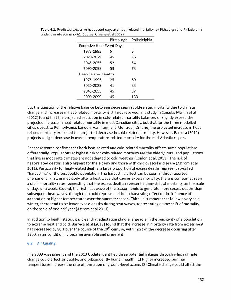
132

Table 6.1. Predicted excessive heat event days and heat-related mortality for Pittsburgh and Philadelphia under climate scenario A1 (Source: Greene et al 2012)

Pittsburgh Philadelphia Excessive Heat Event Days 1975-1995 5 6 2020-2029 45 46 2045-2055 52 54 2090-2099 59 73 Heat-Related Deaths 1975-1995 25 69 2020-2029 41 83 2045-2055 45 97 2090-2099 45 133

But the question of the relative balance between decreases in cold-related mortality due to climate change and increases in heat-related mortality is still not resolved. In a study in Canada, Martin et al (2012) found that the projected reduction in cold-related mortality balanced or slightly exceed the projected increase in heat-related mortality in most Canadian cities, but that for the three modelled cities closest to Pennsylvania, London, Hamilton, and Montreal, Ontario, the projected increase in heat related mortality exceeded the projected decrease in cold-related mortality. However, Barreca (2012) projects a slight decrease in overall temperature-related mortality for the mid-Atlantic region. Recent research confirms that both heat-related and cold-related mortality affects some populations differentially. Populations at highest risk for cold-related mortality are the elderly, rural and populations that live in moderate climates are not adapted to cold weather (Conlon et al. 2011). The risk of heat-related deaths is also highest for the elderly and those with cardiovascular disease (Astrom et al 2011). Particularly for heat-related deaths, a large proportion of excess deaths represent so-called “harvesting” of the susceptible population. The harvesting effect can be seen in three reported phenomena. First, immediately after a heat wave that causes excess mortality, there is sometimes seen a dip in mortality rates, suggesting that the excess deaths represent a time-shift of mortality on the scale of days or a week. Second, the first heat wave of the season tends to generate more excess deaths than subsequent heat waves, though this could represent either a harvesting effect or the influence of adaptation to higher temperatures over the summer season. Third, in summers that follow a very cold winter, there tend to be fewer excess deaths during heat waves, representing a time shift of mortality on the scale of one half year (Astrom et al 2011). In addition to health status, it is clear that adaptation plays a large role in the sensitivity of a population to extreme heat and cold. Barreca et al (2013) found that the increase in mortality rate from excess heat has decreased by 80% over the course of the 20th century, with most of the decrease occurring after 1960, as air conditioning became available and prevalent.

6.2 Air Quality The 2009 Assessment and the 2013 Update identified three potential linkages through which climate change could affect air quality, and subsequently human health. [1] Higher increased summer temperatures increase the rate of formation of ground-level ozone. [2] Climate change could affect the

133

concentration of small airborne particulates. [3] Pollen and mold concentrations could increase as a consequence of climate change. Ground-level ozone is a respiratory irritant that has been linked through epidemiological studies to higher rates of respiratory symptoms (coughing, sneezing, wheezing), aggravation of asthma, and higher rates of respiratory infections, and increased mortality. Ground-level ozone concentrations are highest in summer, when warm temperatures and sunshine facilitate ozone creation from volatile organic compounds. The 2009 Assessment and the 2013 Update concluded that higher summer temperatures due to climate change would be expected to result in more ozone creation, and higher concentrations, resulting in more respiratory morbidity and mortality. Subsequent research has confirmed this conclusion. Sheffield et al. (2011) project that by 2020, climate change will result in increases in the 8-hour maximum ozone concentrations in New York City of 2.7 to 5.3 ppb, which would in turn result in a 7.3% increase in emergency room visits for childhood asthma. Orru et al. (2013) projects that the incidence of ozone-related respiratory illness will increase by 10-14% by 2050 due to climate change. Post et al. (2012) projected the expected change in ozone-related mortality from climate change using several different climate models. They found that most models gave projected increases in ozone-related mortality, but that the size of the increase varied by a factor of 4. While warmer summers will increase ozone formation, the emissions of ozone precursors (including volatile organic compounds and nitrogen oxides) are expected to decline over time as a consequence of tightening emission standards. Lam et al (2011) project that the reduction in emissions will outweigh the increase in summer temperatures in the Northeast U.S., so that maximum ground level ozone concentrations will decline by 10% by 2050. Climate change could affect airborne particulate concentrations, which have been shown to affect both respiratory and cardiovascular health. However, there is no clear consensus on whether climate change will result in an increase or decrease in particulate concentrations. Tai et al (2012) finds that particulate concentrations are correlated with temperature, particularly in the Eastern U.S., but that the relationship is complicated and depends on regional weather patterns. Warmer summers with longer dry spells could also increase the risk of wildfires and of airborne dust from soil, which are important sources of airborne particulates (De Sario 2103). Still, the anticipated increase in particulate concentrations due to climate change is small. Anticipated reductions in emissions from combustion will tend to reduce particulate concentrations in the future by more than any increase due to climate change. Lam et al (2011) project that airborne particulate concentrations could decrease by as much as 40% by 2050, continuing the ongoing downward trend in particulate concentrations. The impact that climate change could have on respiratory allergens such as pollen and molds is not well understood, but it is conjectured that climate change could result in higher pollen loads due to faster plant growth, more pollen produced by each plant, increased allergenicity of the pollen grains, and a longer pollen season (D’Amato et al 2013). Recent warming has caused the ragweed season to lengthen in the Midwest (Ziska et al 2011). Thunderstorms, which are projected to increase in frequency as a result of climate change, have been shown to serve as a trigger for pollen-induced asthma (Dabrera et al 2012).

6.3 Water Quality The two most important pathways that climate change can affect human health through changes in water quality are 1) increased water-borne pathogens from increased water temperature and increased

134

runoff during heavy rain events and 2) increased occurrence of harmful algal blooms in eutrophic lakes due to increased higher nutrient runoff and warmer waters. The risk of disease from water-borne pathogens depends on the concentration of the pathogens in the water and on exposure. Water-borne pathogens pose risk to bathers and to those who use surface water as a drinking source. While public drinking water systems treat drinking water to reduce risk from pathogens, the risk is still there. In 1993, an outbreak of Cryptosporidium in Milwaukee sickened over 400,000 people. Heavy rainfall is thought to have been a factor, coupled with inadequate filtration at one water treatment plant (MacKenzie et al 1994). Climate change can affect the concentration of pathogens in surface waters in complex ways (Hofstra 2011). Higher water temperatures could speed pathogen growth in some cases, but has also been linked to higher rates of inactivation. More extreme precipitation events will cause more surface flow runoff that can carry pathogens into streams and river, particularly from livestock farms, and increase the risk of sewer overflows. More extreme rainfall events will also increase turbulence in rivers and lakes, potentially re-suspending pathogens in sediments (Coffee et al 2014). Finally, dry periods in summer will increase the concentration of pathogens discharged in wastewater. While the potential qualitative impact of climate change on water-borne pathogen concentrations can be conjectured, little research has been conducted that quantitatively measures the size of the potential effect (Hofstra 2011). In summer of 2014, a harmful algal bloom (HAB) occurred in the western basin of Lake Erie. The algal bloom affected the city of Toledo’s water intakes, and 500,000 residents were told to stop using tap water for cooking, drinking or bathing. The algae (a cyanobacteria) produced toxins called microcystins that damage the liver if consumed. Boiling the water does not remove the toxins, so residents were forced to use bottled and trucked water. The bloom also posed health risks to those who bathed in the lake and those who consumed fish caught in the lake. This was the second large bloom in Lake Erie in four years. These recent blooms are the result of a combination of factors, including high nutrient usage (particularly phosphorous) on agricultural fields, high springtime runoff that flushed nutrients into the lake, and then warm, calm weather that allowed the algae to grow without being disrupted by vertical mixing of the lake waters. The meteorological conditions that encouraged the algal blooms in 2011 and 2014 (high spring runoff and warm summers) are expected to become more prevalent with climate change, suggesting these types of blooms will become more common in eutrophic waters (Michalak et al 2013; Paerl and Paul 2012). Harmful algal blooms are more prevalent in warm, shallow lakes than in colder lakes or in rivers. Algal blooms in Lake Erie have tended to be worse in the western basin. Although they do sometimes spread into the central basin of Lake Erie, blooms that cause potential health effects have not yet reached Pennsylvania waters, which tend to be colder, better mixed and less nutrient rich. With continued warming, however, the potential exists for harmful blooms in the Pennsylvania waters of Lake Erie and in inland lakes and reservoirs in the state.

6.4 Extreme Weather Events The greatest risks to human health from extreme weather events are those from heat waves (discussed in Section 7.1) and flooding from severe storms, both tropical cyclones and extra-tropical storms. Hurricane Sandy in 2012 caused 72 direct deaths in the United States, including two in Pennsylvania,

135

making it the deadliest U.S. cyclone outside of the southern states since Hurricane Agnes in 1972 (Blake et al 2013). There is building a consensus in the published literature that climate change will not necessarily increase the frequency of tropical cyclones in the North Atlantic, but that climate change will increase the likelihood that individual storms will be stronger and with heavier rainfall (Villarini and Vecchi 2013; Horton and Liu 2014). Non-tropical extreme rain events have increased in frequency in North American (Kunkel et al 2013) and are projected to continue to increase in frequency as a result of climate change. For the Eastern U.S., a storm with a 24-hour rain total that used to occur with a frequency of once every 20 years is projected to recur every 12 to 16 years by mid-century and every 8-10 years by the end of the century (IPCC 2012), though there are expected to be fewer rain-on-snow events (Chapter 8, this report), However, future risk to human health from flooding will depend more on changes in exposure and vulnerability (where humans choose to live and how they choose to build) than it will on changes in precipitation due to climate change (Kundzewicz 2014). The frequency of severe snowstorms has increased nationally, with the frequency after 1960 double that of the frequency between 1900 and 1960. However, there has not been a detectible trend in the frequency of ice storms for the United States as a whole (Kunkel et al 2013).

6.5 Vector-borne Disease Mosquito-borne diseases, such as malaria, are projected to increase in some lower-income countries as a consequence of climate change, but are not expected to increase higher income countries such as the United States (Beguin et al. 2011). Malaria was endemic in Pennsylvania up through the 1800s but was eradicated by the mid 1900s. Regardless of climate change, malaria is not expected to become re-established in the United States. West Nile disease is endemic in Pennsylvania. It is currently most prevalent in Southeastern and Central parts of the state, and less prevalent in the Laurel Highlands and the Allegheny Plateau. However, climate change is expected to increase the prevalence of West Nile disease in the higher-elevation areas, due to higher temperatures, but decrease its prevalence in the lower elevation areas, due to increased rainfall, which is associated with reduced prevalence of West Nile disease (Figure 6.1). In addition to its range, the duration of the transmission season for West Nile disease is sensitive to climate. Warmer temperatures result in a longer transmission season, and therefore greater infection risk (Chen et al 2013).

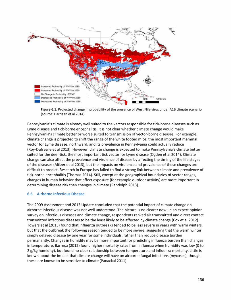
136

Figure 6.1. Projected change in probability of the presence of West Nile virus under A1B climate scenario (source: Harrigan et al 2014)

Pennsylvania’s climate is already well suited to the vectors responsible for tick-borne diseases such as Lyme disease and tick-borne encephalitis. It is not clear whether climate change would make Pennsylvania’s climate better or worse suited to transmission of vector-borne diseases. For example, climate change is projected to shift the range of the white footed mice, the most important mammal vector for Lyme disease, northward, and its prevalence in Pennsylvania could actually reduce (Roy-Dufresne et al 2013). However, climate change is expected to make Pennsylvania’s climate better suited for the deer tick, the most important tick vector for Lyme disease (Ogden et al 2014). Climate change can also affect the prevalence and virulence of disease by affecting the timing of the life stages of the diseases (Altizer et al 2013), but the impacts on virulence and prevalence of these changes are difficult to predict. Research in Europe has failed to find a strong link between climate and prevalence of tick-borne encephalitis (Thomas 2014). Still, except at the geographical boundaries of vector ranges, changes in human behavior that affect exposure (for example outdoor activity) are more important in determining disease risk than changes in climate (Randolph 2013).

6.6 Airborne Infectious Disease The 2009 Assessment and 2013 Update concluded that the potential impact of climate change on airborne infectious disease was not well understood. The picture is no clearer now. In an expert opinion survey on infectious diseases and climate change, respondents ranked air transmitted and direct contact transmitted infectious diseases to be the least likely to be affected by climate change (Cox et al 2012). Towers et al (2013) found that influenza outbreaks tended to be less severe in years with warm winters, but that the outbreak the following season tended to be more severe, suggesting that the warm winter simply delayed disease by one year for some individuals, rather than reduce disease burden permanently. Changes in humidity may be more important for predicting influenza burden than changes in temperature. Barreca (2012) found higher mortality rates from influenza when humidity was low (0 to 2 g/kg humidity), but found no clear relationship between temperature and influenza mortality. Little is known about the impact that climate change will have on airborne fungal infections (mycoses), though these are known to be sensitive to climate (Panackal 2011).

137

6.7 Adaptation Opportunities and Barriers For almost every human health risk discussed in this chapter, there is a non-climate stressor or factor that mediates the relationship between climate and the health risk. For example:

• Respiratory and cardiovascular disease associated with ozone and airborne particulates are sensitive to climate change, but are more sensitive to air pollutant emissions than climate.

• The weather patterns that favor harmful algal blooms are more likely to happen with climate change, but the risk of HABs is more sensitive to nutrient runoff than climate.

• The prevalence and distribution of vector-borne diseases could be affected by climate change (in complex, difficult to predict ways), but the disease burden from vector-borne diseases will depend more on behavior (outdoor activity) and access to health care.

• Risk from flood events is likely to increase due to climate change, but is more sensitive to where and how people settle on the landscape than to climate

In each case, there are adaptation opportunities that will mitigate the impact that climate change will have on human health. A common adaptation strategy when health risks are due to multiple stressors is to reduce stressors other than climate. For example, to minimize the risk of harmful algal blooms in the face of a warming climate, reduce nutrient runoff. To minimize the risk of water-borne pathogens in the face of increased frequency of extreme precipitation events, control runoff from livestock operations and maintain drinking water treatment facilities. To reduce respiratory and cardiovascular disease from air pollution in the face of a warming climate, reduce emissions of air pollutants. To reduce flood risk in the face of increased extreme precipitation events, build out the landscape in a way that puts humans and infrastructure at less risk. The incidence of vector-borne disease could change as climate changes, but is more sensitive to how much time people spend in outdoor activities and where they spend that time. Public education to minimize infection risk could reduce disease burden. Access to health care will reduce the severity of vector-borne diseases when they are contracted. Adaptation strategies to reduce heat-related mortality include 1) improve air quality, which is a contributing factor to heat-related disease, 2) provide cooling shelters to low income residents who cannot afford air conditioning, and 3) public education and alert systems, so that residents can plan for heat waves (Kravchenko et al 2013).

References Altizer, S., Ostfield, R.S., Johnson, P.T.J., Kutz, S., & Harvell, C.D., (2013). Climate Change and Infectious

Diseases: From Evidence to a Predictive Framework. Science 341(6145), 514-519. Astrom, D.O., Forsberg, B., & Rocklov, J., (2011). Heat wave impact on morbidity and mortality in the

elderly population: A review of recent studies. Maturitas 69, 99-105. Barreca, A.I. (2012). Climate change, humidity, and mortality in the United States. Journal of

Environmental Economics and Management 63, 19-34. Barrece, A., Clay, K., Deschenes, O., Greenstone, M., & Shapiro, J.S. (2013). Adapting to Climate Change:

The Remarkable Decline in the U.S. Temperature-Mortality Relationship over the 20th Century. National Bureau of Economic Research Working Paper 18692. Cambridge, MA.

138

Beguin, A., Hales, S., Rocklov, J., Astrom, C., Louis, V.R., & Sauerborn, R. (2011). The opposing effects of climate change and socio-economic development on the global distribution of malaria. Global Environmental Change 21(4), 1209-1214.

Blake, E.S., Kimberlain, T.B., Berg, R.J., Cangialosi, J.P., & Beven, J.L. (2013). Tropical Cyclone Report: Hurricane Sandy. National Hurricane Center, NOAA.

Chen, S., Blanford, J.I., Fleischer, S.J., Hutchinson, M., Saunders, M.C., & Thomas, M.B. (2013). Estimating West Nile Virus Transmission Period in Pennsylvania Using an Optimized Degree-Day Model. Vector Borne and Zoonotic Diseases 13(7), 489-497.

Coffee, R., Benham, B., Krometis, L.A., Wolfe, M.L., & Cummins, E. (2014). Assessing the Impact of Climate Change and Land Use Variation on Microbial Transport Using Watershed-scale Modeling. Online Journal of Public Health Informatics 6(1):e15, 2014

Conlon, K.C., Rajkovich, N.B., White-Newsome, J.L., Larsen, L., & O’Neill, M.S. (2011). Preventing cold-related morbidity and mortality in a changing climate. Maturitas 69, 197-202.

Cox, R., Revie, C.W., & Sanchez, J. (2012). The Use of Expert Opinion to Assess the Risk of Emergence or Re-emergence of Infectious Diseases in Canada Associated with Climate Change. PLOS One DOI: 10.1371/journal.pone.0041590

D’Amato, G., Baena-Cagnani, C.E., Cecchi, L., Annesi-Maesano, I., Nunes, C., Ansotegui, I., D’Amato, M., Liccardi, G., Sofia, M., & Canonica, W.G. (2013). Multidisciplinary Respiratory Medicine 8:12,

Dabrera, G., Murray, V., Emberlin, J., Ayres, J.G., Collier, C., Clewlow, Y., & Sachon, P. (2012). Thunderstorm asthma: an overview of the evidence base and implications for public health advice. QJM: An International Journal of Medicine doi:10.1093/qjmed/hcs234

De Sario, M., Katsouyanni, K., & Michelozzi, P., (2013). Climate Change, Extreme Weather Events, and Respiratory Health in Europe. European Respiratory Journal doi: 10.1183/09031936.00074712

Greene, S., Kalkstein, L.S., Mills, D.M., & Samenow, J. (2011). An Examination of Climate Change on Extreme Heat Events and Climate-Mortality Relationships in Large U.S. Cities. Weather, Climate and Society 3, 281-292.

Harrigan, R.J., Thomassen, H.J., Beurmann, W., & Smith, T.B. (2014). A Continental Risk Assessment of West Nile Virus Under Climate Change. Global Change Biology 20(8), 2417-2425.

Hofstra, N. (2011). Quantifying the impact of climate change on enteric waterborne pathogen concentrations in surface water. Current Opinion in Environmental Sustainability 3, 471-479.

Horton, R.M., & Liu, J.P. (2014) Beyond Hurricane Sandy: What might the future hold for tropical cyclones in the North Atlantic? Journal of Extreme Events 1(1), 1450007, doi:10.1142/ S2345737614500079.

IPCC (2012). Managing the Risks of Extreme Events and Disasters to Advance Climate Change Adaptation. A Special Report of Working Groups I and II of the Intergovernmental Panel on Climate Change [Field, C.B., V. Barros, T.F. Stocker, D. Qin, D.J. Dokken, K.L. Ebi, M.D. Mastrandrea, K.J. Mach, G.-K. Plattner, S.K. Allen, M. Tignor, and P.M. Midgley (eds.)]. Cambridge University Press, Cambridge, UK, and New York, NY, USA, 582 pp.

Kravchenko, J., Abernethy, A.P., Fawzy, M., & Lyerly, H.K. (2013). Minimization of Heatwave Morbidity and Mortality. American Journal of Preventive Medicine 44(3), 274-282.

Kundzewicz, Z.W., Kanae, S., Seneviratne, S.I., Handmer, J., Nicholls, N., Peduzzi, P., Mechler, R., Bouwer, L.M., Arnell, N., Mach, K., Muir-Wood, R., Brakenridge, G.R., Kron, W., Benito, G., Honda, Y., Takahashi, K., & Sherstyukov, B. (2014). Flood risk and climate change: global and regional perspectives. Hydrological Sciences Journal 59(1), 1-28.

139

Kunkel, K.E., Karl, T.R., Brooks, H., Kossin, J., Lawrimore, J.H., Arndt, D., Bosart, L., Changnon, D., Cutter, S.L., Doesken, N., Emanuel, K., Groisman, P.Y., Katz, R.W., Knutson, T., O'Brien, J., Paciorek, C.J., Peterson, T.C., Redmond, K., Robinson, D., Trapp, J., Vose, R., Weaver, S., Wehner, M., Wolter, K., & Wuebbles, D. (2013) Monitoring and Understanding Trends in Extreme Storms: State of Knowledge. Bulletin of the American Meteorological Society, 94, 499–514.

Lam, Y.F., Fu, J.S., Wu, S., & Mickley, L.J. (2011). Impacts of future climate change and effects of biogenic emissions on surface ozone and particulate matter concentrations in the United States. Atmospheric Chemistry and Physics 11, 4789-4806.

MacKenzie, W.R., Hoxie, N.J., Proctor, M.E., Gradus, M.S., Blair, K.A., Peterson, D.E., Kazmierczak, J.J., Addiss, D.G., Fox, K.R., Rose, J.B., & Davis, J.P. (1994). A Massive Outbreak of Cryptosporidium Infection Transmitted Through the Public Water Supply. New England Journal of Medicine 331(3), 161-167.

Martin, S.L., Cakmak, S., Hebbern, C.A., Avramescu, M.L., & Tremblay, N. (2012). Climate change and future temperature-related mortality in 15 Canadian cities. International Journal of Biometeorology 56, 605-619.

Michalak, A.M., Anderson, E.J., Deletsky, D., Boland, S., Bosch, N.S., Bridgeman, T.B., Chaffin, J.D., Cho, K., Confesor, R., Daloglu, I., DePinto, J.V., Evans, M.A., Fahnensteil, G.L., He, L., Ho, J.C., Jenkins, L., Johengen, T.H., Kuo, K.C., LaPorte, E., Liu, X., McWilliams, M.R., Moore, M.R., Posselt, D.J., Richard, R.P., Scavia, D., Steiner, A.L., Verhamme, E., Wright, D.M., & Zagorski, M.A. (2013). Record-setting algal bloom in Lake Erie caused by agricultural and meteorological trends consistent with expected future conditions. Proceedings of the National Academy of Sciences 110(16), 6448-6452.

Ogden, N.H., Radojevic, M., Wu, X., Duvvuri, V.R., Leighton, P.A., & Wu, J. (2014). Estimated Effects of Projected Climate Change on the Basic Reproductive Number of the Lyme Disease Vector Ixodes scapularis. Environmental Health Perspectives 122(6), 631-638.

Orru, H., Andersson, C., Ebi, K.L., Langner, J., Astrom, C., & Forsberg, B. (2013). Impact of climate change on ozone-related mortality and morbidity in Europe. European Respiratory Journal 41, 295-294.

Paerl, H.W., & Paul, V.J. (2012). Climate change: Links to global expansion of harmful cyanobacteria. Water Research 5(1), 1349-1363.

Panackal, A.A. (2011). Global Climate Change and Infectious Diseases: Invasive Mycoses. Journal of Earth Science and Climatic Change 1:108 doi:10.4172/2157-7617.1000108

Post, E.S., Grambsch, A., Weaver, C., Morefield, P., Huang, J., Leung, L.Y., Nolte, C.G., Adams, P., Liang, X.Z., Zhu, J.H., & Mahoney, H. (2012). Variation in Estimated Ozone-Related Health Impacts of Climate Change due to Modeling Choices and Assumptions. Environmental Health Perspectives 120(11), 1559-1564.

Randolph, S.E. (2013). Is expert opinion enough? A critical assessment of the evidence for potential impacts of climate change on tick-borne diseases. Animal Health Research Reviews 14(2), 133-137.

Roy-Dufresne, E., Logan, T., Simon, J.A., Chmura, G.L., & Millien, V., (2013). Poleward Expansion of the White-Footed Mouse (Peromyscus leucopus) under Climate Change: Implications for the Spread of Lyme Disease. PLOS One DOI: 10.1371/journal.pone.0080724

Sheffield, P.E., Knowlton, K., Carr, J.L., & Kinney, P.L. (2011). Modeling of Regional Climate Change Effects on Ground Level Ozone. American Journal of Preventive Medicine 41(3), 251-257.

Tai, A.P.K., Mickley, L.J., & Jacob, D.J. (2012). Impact of 2000-2050 climate change on fine particulate matter (PM2.5) air quality inferred from a multi-model analysis of meteorological modes. Atmospheric Chemistry and Physics 12, 11329-11337.

Thomas, P.R. (2014). Tick-Borne Encephalitis Transmission Risk: Its Dependence on Host Population Dynamics and Climate Effects. Vector-Borne and Zoonotic Diseases 14(5), 346-352.

140

Towers, S., Chowell, G., Hameed, R., Jastrebski, M., Khan, M., Meeks, J., Mubayi, A., & Harris, G. (2013). Climate change and influenza: the likelihood of early and severe influenza seasons following warm winters. PLOS Currents doi: 10.1371/currents.flu.3679b56a3a5313dc7c043fb944c6f138

Villarini, G., & Vecchi, G.A. (2013). Projected Increases in North Atlantic Tropical Cyclone Intensity from CMIP5 Models. Journal of Climate 26, 3231-3240.

Ziska, L., Knowlton, K., Rogers, C., Dalan, D., Tierney, N., Elder, M.A., Filley, W., Shropshire, J., Ford, L.B., Hedberg, C., Fleetwood, P., Hovanky, K.T., Kavanaugh, T., Fulford, G., Vrtis, R.F., Patz, J.A., Portney, J., Coates, F., Bielory, L., & Frenz, D. (2011). Recent warming by latitude associated with increased length ragweed pollen season in central North America. Proceedings of the National Academy of Sciences 108(10), 4248-4251.

141

7 Outdoor Recreation

7.1 Introduction Chapter 12 of the 2009 Pennsylvania Climate Impacts Assessment (2009 Assessment) and Chapter 10 of the 2013 Pennsylvania Climate Impacts Assessment Update (2013 Update) reviewed available information on the potential impacts of climate change on outdoor recreation and tourism in Pennsylvania. Those reviews concluded that climate change would affect outdoor recreation in several ways. The most important impacts identified were:

1. Higher spring and fall temperatures will lengthen the outdoor recreation season resulting in a general increase in outdoor recreation participation;

2. Higher summer temperatures will particularly increase demand for water-based recreation; 3. Higher summer temperatures will decrease the amount of habitat suitable for trout in

Pennsylvania, but total participation in recreational fishing may increase, because of the longer season;

4. Reduced summer streamflows could negatively affect sport fish populations; 5. Higher winter temperatures and reduced snowfall will negatively impact snow-based recreation

such as skiing and snowmobiling. In this chapter we review research that has been conducted since the 2013 Update.

7.2 National Estimates of Changes in Outdoor Recreation Since 1960, the US Forest Services has periodically conducted a survey now called the National Survey on Recreation and the Environment (NSRE). The most recent survey was conducted in 2010. This is a telephone survey of U.S. households asking about their participation in outdoor, resource-based recreation. While the survey cannot be used to track changes in recreation that have occurred as a result of climate change since 1960, it can be used to determine whether recreation participation is correlated with spatial differences in climate. For example, the survey will reveal whether households who live in warmer areas participate in outdoor recreation more or less frequently than household who live in cooler areas. This is the approach that was taken by Bowker et al (2012), who estimated statistical models of outdoor recreation behavior. The models included information on the household surveyed (income, age, ethnicity) as well as the climate and other geographic information about the location of the household’s residence. For seventeen different outdoor recreation activities, Bowker et al. estimated models that explain differences in participation rates (whether the household engaged in the activity at all) and frequency (for households that engage in the activity, how many days per year). For each activity, the authors included in the models the climate measure that best explained variation. For most outdoor recreation activities, the authors projected increases in the total number of participant days nationally of 40 to 80%, both with and without climate change factored in. This is mostly due to population growth and increases in household income. Pennsylvania’s population is projected to grow more slowly than the national average, so increases in outdoor recreation in Pennsylvania will be smaller than those projected by Bowker et al.

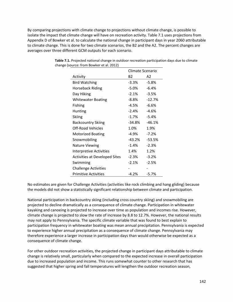
142

By comparing projections with climate change to projections without climate change, is possible to isolate the impact that climate change will have on recreation activity. Table 7.1 uses projections from Appendix D of Bowker et al. to calculate the national change in participant days in year 2060 attributable to climate change. This is done for two climate scenarios, the B2 and the A2. The percent changes are averages over three different GCM outputs for each scenario.

Table 7.1. Projected national change in outdoor recreation participation days due to climate change (source: from Bowker et al. 2012)

Climate Scenario Activity B2 A2 Bird Watching -3.3% -5.8% Horseback Riding -5.0% -6.4% Day Hiking -2.1% -3.5% Whitewater Boating -8.8% -12.7% Fishing -4.5% -6.6% Hunting -2.4% -4.6% Skiing -1.7% -5.4% Backcountry Skiing -34.8% -46.1% Off-Road Vehicles 1.0% 1.9% Motorized Boating -4.9% -7.2% Snowmobiling -43.2% -53.5% Nature Viewing -1.4% -2.3% Interpretive Activities 1.4% 1.2% Activities at Developed Sites -2.3% -3.2% Swimming -2.1% -2.5% Challenge Activities - - Primitive Activities -4.2% -5.7%

No estimates are given for Challenge Activities (activities like rock climbing and hang gliding) because the models did not show a statistically significant relationship between climate and participation. National participation in backcountry skiing (including cross country skiing) and snowmobiling are projected to decline dramatically as a consequence of climate change. Participation in whitewater kayaking and canoeing is projected to increase over time as population and incomes rise. However, climate change is projected to slow the rate of increase by 8.8 to 12.7%. However, the national results may not apply to Pennsylvania. The specific climate variable that was found to best explain to participation frequency in whitewater boating was mean annual precipitation. Pennsylvania is expected to experience higher annual precipitation as a consequence of climate change. Pennsylvania may therefore experience a larger increase in participation days than would otherwise be expected as a consequence of climate change. For other outdoor recreation activities, the projected change in participant days attributable to climate change is relatively small, particularly when compared to the expected increase in overall participation due to increased population and income. This runs somewhat counter to other research that has suggested that higher spring and fall temperatures will lengthen the outdoor recreation season,

143

increasing total participation. Again, because the Bowker et al. study is national in scope, it includes areas where high heat may be a limiting factor in participation. It is of particular interest to note that the projected impact of climate change on participation in downhill skiing and snowboarding is relatively small. The authors did find that participation in downhill skiing and snowboarding was negatively correlated with winter temperatures at the survey respondent’s residence, but the relationship was not strong enough to suggest large impacts on participation. Part of this could be because the survey does not distinguish between skiing that occurs near the respondent’s residence and skiing that occurs at destination resorts in colder climates.

7.3 Winter Recreation The 2009 Assessment and 2013 Update identified winter recreation as the outdoor recreation activity most sensitive to climate change, because of its reliance on ice and snow. Previous research has shown that commercial downhill ski areas can adapt to climate change by increasing investment in snowmaking, but that there are limits to snowmaking to replace natural snowfall. Snowmaking requires temperatures low enough to allow the sprayed water to freeze. The 2009 Assessment and the 2013 Update reviewed published literature that showed that Pennsylvania ski resorts will experience shorter seasons, higher snowmaking costs, and lower profits as a consequence of climate change. Recent research has reached similar results. Dawson and Scott (2013) projected the impact of climate change on ski area operations in New York and New England states (Pennsylvania ski areas were not included in the study). They evaluated which ski areas would still be economically viable under different climate scenarios. Their definition of an economically viable ski area was one that could maintain an average season length of 100 days and a 75% probability of being open over the winter holiday season. Using that criterion, with one exception, only ski areas in Maine, New Hampshire, Vermont and the Adirodack Mountains of New York are projected to remain economically viable through mid-century. This result was true both under the B1 and the A1fi scenarios. The one ski area location south of the Adirondack Mountains that was projected to remain economically viable was Bobcat Ski Center, in the western Catskills.1 While no ski areas remained viable in southern or western New York under either climate scenario, the survival of more northern ski areas was sensitive to the climate scenario analyzed. For example, under the B1 (lower emissions) scenario, seven ski areas in northern New York are projected to be economically viable through the end of the century. Under the A1fi (higher emissions) scenario, only two are. While snowfall and temperatures low enough to make snow are important factors in determining the economic viability of ski areas, they are not the only factors. A study pf resort closings in Austria (Falk 2013) found that adoption of snowmaking was an important factor in maintaining viability, but that regional effects (customer base) and macroeconomic effects were at least as important as snowfall in predicting which resorts would close. The implication for Pennsylvania is that resorts located closer to cities will be able to maintain viability longer. A second implication is that closures are more likely to occur during economic downturns.

1 Unfortunately, Bobcat Ski Center has been closed since the end of the 2005 ski season. Bobcat was a small ski area that chose not to invest in modern snowmaking equipment.

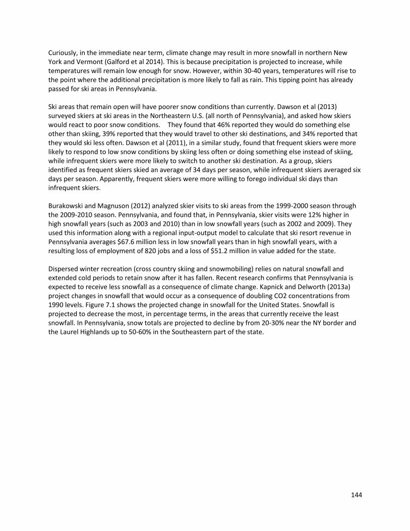
144

Curiously, in the immediate near term, climate change may result in more snowfall in northern New York and Vermont (Galford et al 2014). This is because precipitation is projected to increase, while temperatures will remain low enough for snow. However, within 30-40 years, temperatures will rise to the point where the additional precipitation is more likely to fall as rain. This tipping point has already passed for ski areas in Pennsylvania. Ski areas that remain open will have poorer snow conditions than currently. Dawson et al (2013) surveyed skiers at ski areas in the Northeastern U.S. (all north of Pennsylvania), and asked how skiers would react to poor snow conditions. They found that 46% reported they would do something else other than skiing, 39% reported that they would travel to other ski destinations, and 34% reported that they would ski less often. Dawson et al (2011), in a similar study, found that frequent skiers were more likely to respond to low snow conditions by skiing less often or doing something else instead of skiing, while infrequent skiers were more likely to switch to another ski destination. As a group, skiers identified as frequent skiers skied an average of 34 days per season, while infrequent skiers averaged six days per season. Apparently, frequent skiers were more willing to forego individual ski days than infrequent skiers. Burakowski and Magnuson (2012) analyzed skier visits to ski areas from the 1999-2000 season through the 2009-2010 season. Pennsylvania, and found that, in Pennsylvania, skier visits were 12% higher in high snowfall years (such as 2003 and 2010) than in low snowfall years (such as 2002 and 2009). They used this information along with a regional input-output model to calculate that ski resort revenue in Pennsylvania averages $67.6 million less in low snowfall years than in high snowfall years, with a resulting loss of employment of 820 jobs and a loss of $51.2 million in value added for the state. Dispersed winter recreation (cross country skiing and snowmobiling) relies on natural snowfall and extended cold periods to retain snow after it has fallen. Recent research confirms that Pennsylvania is expected to receive less snowfall as a consequence of climate change. Kapnick and Delworth (2013a) project changes in snowfall that would occur as a consequence of doubling CO2 concentrations from 1990 levels. Figure 7.1 shows the projected change in snowfall for the United States. Snowfall is projected to decrease the most, in percentage terms, in the areas that currently receive the least snowfall. In Pennsylvania, snow totals are projected to decline by from 20-30% near the NY border and the Laurel Highlands up to 50-60% in the Southeastern part of the state.

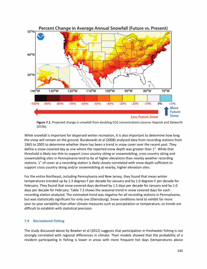
145

Figure 7.1. Projected change in snowfall from doubling CO2 concentrations (source: Kapnick and Delworth 2013b).

While snowfall is important for dispersed winter recreation, it is also important to determine how long the snow will remain on the ground. Burakowski et al (2008) analyzed data from recording stations from 1965 to 2005 to determine whether there has been a trend in snow cover over the recent past. They define a snow-covered day as one where the reported snow depth was greater than 1”. While that threshold is likely too thin to support cross country skiing or snowmobiling, cross country skiing and snowmobiling sites in Pennsylvania tend to be at higher elevations than nearby weather recording stations. 1” of cover at a recording station is likely closely correlated with snow depth sufficient to support cross country skiing and/or snowmobiling at nearby, higher elevation sites. For the entire Northeast, including Pennsylvania and New Jersey, they found that mean winter temperatures trended up by 1.3 degrees F per decade for January and by 1.0 degrees F per decade for February. They found that snow-covered days declined by 1.5 days per decade for January and by 1.0 days per decade for February. Table 7.2 shows the seasonal trend in snow covered days for each recording station analyzed. The estimated trend was negative for all recording stations in Pennsylvania, but was statistically significant for only one (Ebensburg). Snow conditions tend to exhibit far more year-to-year variability than other climate measures such as precipitation or temperature, so trends are difficult to establish with statistical precision.

7.4 Recreational Fishing The study discussed above by Bowker et al (2012) suggests that participation in freshwater fishing is not strongly correlated with regional differences in climate. Their models showed that the probability of a resident participating in fishing is lower in areas with more frequent hot days (temperatures above

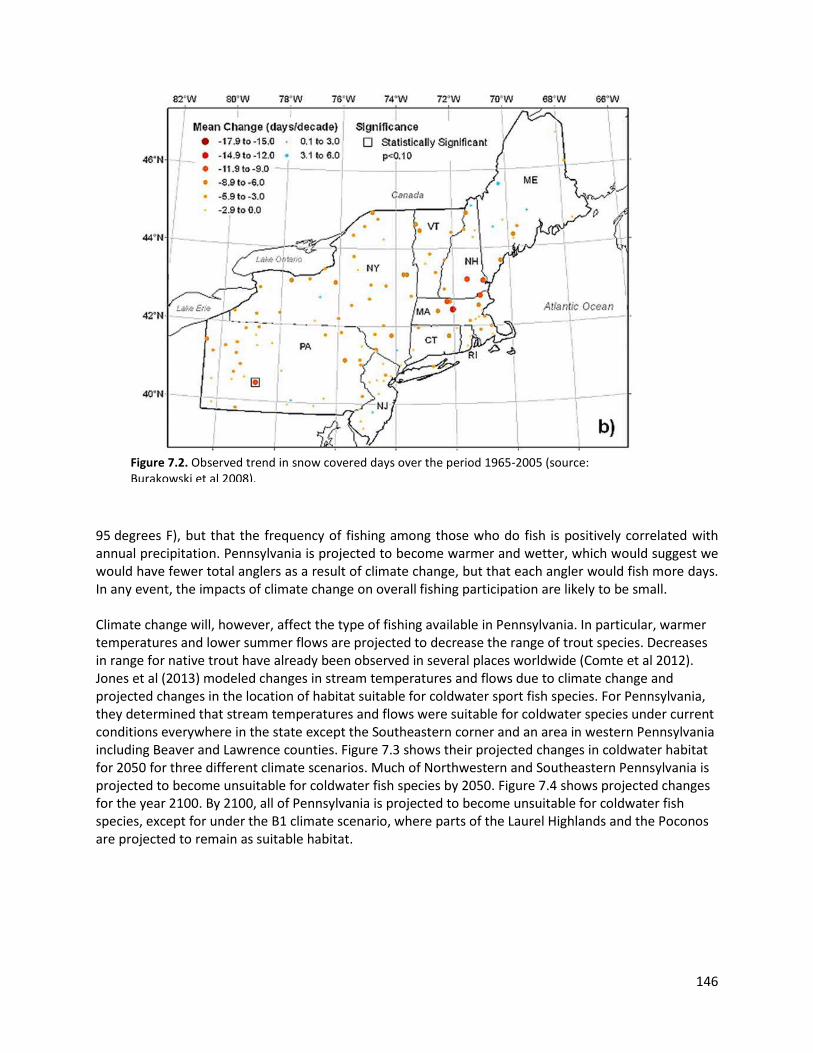
146

95 degrees F), but that the frequency of fishing among those who do fish is positively correlated with annual precipitation. Pennsylvania is projected to become warmer and wetter, which would suggest we would have fewer total anglers as a result of climate change, but that each angler would fish more days. In any event, the impacts of climate change on overall fishing participation are likely to be small. Climate change will, however, affect the type of fishing available in Pennsylvania. In particular, warmer temperatures and lower summer flows are projected to decrease the range of trout species. Decreases in range for native trout have already been observed in several places worldwide (Comte et al 2012). Jones et al (2013) modeled changes in stream temperatures and flows due to climate change and projected changes in the location of habitat suitable for coldwater sport fish species. For Pennsylvania, they determined that stream temperatures and flows were suitable for coldwater species under current conditions everywhere in the state except the Southeastern corner and an area in western Pennsylvania including Beaver and Lawrence counties. Figure 7.3 shows their projected changes in coldwater habitat for 2050 for three different climate scenarios. Much of Northwestern and Southeastern Pennsylvania is projected to become unsuitable for coldwater fish species by 2050. Figure 7.4 shows projected changes for the year 2100. By 2100, all of Pennsylvania is projected to become unsuitable for coldwater fish species, except for under the B1 climate scenario, where parts of the Laurel Highlands and the Poconos are projected to remain as suitable habitat.

Figure 7.2. Observed trend in snow covered days over the period 1965-2005 (source: Burakowski et al 2008).

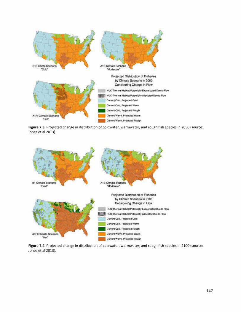
147

Figure 7.3. Projected change in distribution of coldwater, warmwater, and rough fish species in 2050 (source: Jones et al 2013).

Figure 7.4. Projected change in distribution of coldwater, warmwater, and rough fish species in 2100 (source: Jones et al 2013).

148

7.5 Water-Based Recreation The 2009 Assessment and the 2013 Update suggested that higher summer temperatures and warmer spring and fall temperatures would result in more participation in water-based outdoor recreation, particularly swimming and bathing in lakes and rivers. In the analysis by Bowker et al. (2012), it was found that higher temperatures increased the likelihood that a resident participated in swimming, but decreased the frequency of participation for residents who go swimming at least once. The net effect, nationally, is a small decrease in swimming as a consequence of climate change. That analysis, however, did not control for regional differences in water quality that may have been correlated with regional differences in climate. Climate, and climate change, can affect water quality in important ways (Murdoch et al 2000). For example, higher evapotranspiration due to higher summertime temperature are expected to lead to reduced summer streamflows, and increased potential for eutrophication due to higher nutrient concentrations (from less dilution) and higher productivity. This in turn can lead to lower dissolved oxygen levels. A particular concern regarding water quality is the potential increase in the prevalence of harmful algal blooms, like the bloom that occurred in western Lake Erie near Toledo in summer 2014. Climate change is expected to result in warmer summer temperatures, flashier hydrology, and increased eutrophication, which together favor increases in the occurrence of harmful algal blooms (Paerl and Huisman 2009; Oneil et al 2011).

7.6 Outdoor Sports and Exercise Activities In the 2009 Assessment and the 2013 Update, evidence was provided that suggests that frequency of participation in outdoor sports and exercise activities (golf, running, bicycling, soccer, etc.) will increase in spring and fall, as those seasons become warmer, but that participation in these activities is limited by heat only at very high temperatures. Recent research is consistent with that finding. Zivin and Neidell (2014) use data from the American Time Use Survey to investigate the relationship between daily behavior and weather. Figure 7.5 shows how time spent working, in outdoor leisure, and in indoor leisure vary with daytime maximum temperature. The relationships shown in Figure 1 are adjusted to account for differences in day length, so the pattern is due only to differences in temperature, not season. Time spent working is relatively insensitive to temperature except at higher temperatures. Above, 85 degrees F, time spent working decreases as daytime maximum temperature increases. Ziving and Neidell found that this relationship was particularly strong for people who work in outdoor jobs such as agriculture, forestry, mining and construction. Time spent in outdoor leisure increases as temperature increases up to about 75 degrees F. On average, people spend 37 minutes more per day in outdoor leisure at 75-80 degrees F than at 25 degrees F. Time spent in outdoor leisure is fairly stable between temperatures of 75 degrees and 100 degrees F, and only drops when daytime high temperatures exceed 100 degrees F. Currently, days with maximum temperature over 100 degrees F are rare in Pennsylvania (fewer than 1 per year on average). However, by 2100, Philadelphia is projected to experience between 6 and 25 days per year with temperature exceeding 100 degrees, depending on the emissions scenario (UCS 2008). Other Pennsylvania cities will experience slightly fewer such hot days, but even Erie is projected to face 3 to 16 days with maximum temperatures above 100 degrees F.

149

Figure 7.5. Time spent working, in outdoor leisure, and in indoor leisure as a function of daytime maximum temperature (source: Zivin and Neidell 2014).

While higher temperatures, by themselves, are expected to affect outdoor leisure only on the hottest days, increased temperatures can lead to higher concentrations of ozone and pollen, which can exacerbate respiratory illness, including asthma, and further limit outdoor activity (Barnes et al 2013). An important consideration in predicting changes in outdoor leisure activity in response to climate change is the design of outdoor spaces. Chen and Ng (2012) point out that while air temperature and solar radiation are important predictors of duration of outdoor use, design (location of seating and shade, for example) also plays an important role.

7.7 Adaptation Opportunities and Barriers Participation in outdoor recreation, measured in user days, is expected to increase over the century, mostly due to increases in population and incomes. Regardless of the future climate, Pennsylvania needs to plan for and capitalize on increased demand for outdoor recreation. For most outdoor recreation activities, the impact of climate on participation is expected to be small. The important exception is winter activities (downhill skiing, snowboarding, cross country skiing, snowmobiling, ice skating). Participation in these activities is projected to decline due to higher winter temperatures, lower snowfall, and increased snow melt. Developed downhill ski areas can maintain viability by investing in snowmaking, but are not expected to remain economically viable past mid-century. Individual winter sports enthusiasts will respond by travelling farther to reach destinations that still provide winter recreation opportunities and by engaging in winter recreation less frequently, switching to alternative activities. In many cases, negative impacts on outdoor recreation from climate change are due to a combination of climate change and other stressors. Outdoor activity is likely to be limited by worsened air quality that will occur as the result of higher temperatures combined with air emissions. Swimming in lakes and rivers can be limited by poor water quality that is the result of higher temperatures, lower summer

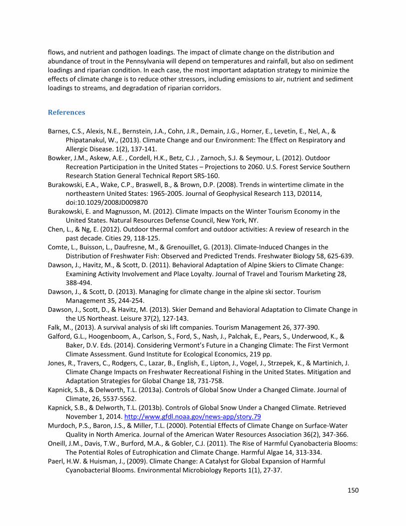
150

flows, and nutrient and pathogen loadings. The impact of climate change on the distribution and abundance of trout in the Pennsylvania will depend on temperatures and rainfall, but also on sediment loadings and riparian condition. In each case, the most important adaptation strategy to minimize the effects of climate change is to reduce other stressors, including emissions to air, nutrient and sediment loadings to streams, and degradation of riparian corridors.

References Barnes, C.S., Alexis, N.E., Bernstein, J.A., Cohn, J.R., Demain, J.G., Horner, E., Levetin, E., Nel, A., &

Phipatanakul, W., (2013). Climate Change and our Environment: The Effect on Respiratory and Allergic Disease. 1(2), 137-141.

Bowker, J.M., Askew, A.E. , Cordell, H.K., Betz, C.J. , Zarnoch, S.J. & Seymour, L. (2012). Outdoor Recreation Participation in the United States – Projections to 2060. U.S. Forest Service Southern Research Station General Technical Report SRS-160.

Burakowski, E.A., Wake, C.P., Braswell, B., & Brown, D.P. (2008). Trends in wintertime climate in the northeastern United States: 1965-2005. Journal of Geophysical Research 113, D20114, doi:10.1029/2008JD009870

Burakowski, E. and Magnusson, M. (2012). Climate Impacts on the Winter Tourism Economy in the United States. Natural Resources Defense Council, New York, NY.

Chen, L., & Ng, E. (2012). Outdoor thermal comfort and outdoor activities: A review of research in the past decade. Cities 29, 118-125.

Comte, L., Buisson, L., Daufresne, M., & Grenouillet, G. (2013). Climate-Induced Changes in the Distribution of Freshwater Fish: Observed and Predicted Trends. Freshwater Biology 58, 625-639.

Dawson, J., Havitz, M., & Scott, D. (2011). Behavioral Adaptation of Alpine Skiers to Climate Change: Examining Activity Involvement and Place Loyalty. Journal of Travel and Tourism Marketing 28, 388-494.

Dawson, J., & Scott, D. (2013). Managing for climate change in the alpine ski sector. Tourism Management 35, 244-254.

Dawson, J., Scott, D., & Havitz, M. (2013). Skier Demand and Behavioral Adaptation to Climate Change in the US Northeast. Leisure 37(2), 127-143.

Falk, M., (2013). A survival analysis of ski lift companies. Tourism Management 26, 377-390. Galford, G.L., Hoogenboom, A., Carlson, S., Ford, S., Nash, J., Palchak, E., Pears, S., Underwood, K., &

Baker, D.V. Eds. (2014). Considering Vermont’s Future in a Changing Climate: The First Vermont Climate Assessment. Gund Institute for Ecological Economics, 219 pp.

Jones, R., Travers, C., Rodgers, C., Lazar, B., English, E., Lipton, J., Vogel, J., Strzepek, K., & Martinich, J. Climate Change Impacts on Freshwater Recreational Fishing in the United States. Mitigation and Adaptation Strategies for Global Change 18, 731-758.

Kapnick, S.B., & Delworth, T.L. (2013a). Controls of Global Snow Under a Changed Climate. Journal of Climate, 26, 5537-5562.

Kapnick, S.B., & Delworth, T.L. (2013b). Controls of Global Snow Under a Changed Climate. Retrieved November 1, 2014. http://www.gfdl.noaa.gov/news-app/story.79

Murdoch, P.S., Baron, J.S., & Miller, T.L. (2000). Potential Effects of Climate Change on Surface-Water Quality in North America. Journal of the American Water Resources Association 36(2), 347-366.

Oneill, J.M., Davis, T.W., Burford, M.A., & Gobler, C.J. (2011). The Rise of Harmful Cyanobacteria Blooms: The Potential Roles of Eutrophication and Climate Change. Harmful Algae 14, 313-334.

Paerl, H.W. & Huisman, J., (2009). Climate Change: A Catalyst for Global Expansion of Harmful Cyanobacterial Blooms. Environmental Microbiology Reports 1(1), 27-37.

151

Union of Concerned Scientists (UCS) (2008). Climate Change in Pennsylvania: Impacts and Solutions for the Keystone State. Cambridge, MA.

Zivin, J.G., & Neidell, M. (2014). Temperature and Allocation of Time: Implications for Climate Change. Journal of Labor Economics 32(1), 1-26.

152

8 Water Resources

8.1 Introduction This chapter is an update on Chapter 5 of the 2013 Pennsylvania Climate Impacts Assessment. The table below summarizes the projections made in the past report: Table 8.1. Summary of projections for Pennsylvania water resources, reprinted from Table 5.3 of the 2013 Pennsylvania Climate Impact Assessment.

Since projected changes in the water cycle over the next few decades are continued increases in temperature and precipitation (Stocker et al., 2013, also Section 2 of this report), it is important to examine past, substantiated change trends to make informed decisions for the future. Recently, research activities in hydrologic science have been profoundly transformed by the availability of (a) large-scale satellite-based observations of various aspects of the hydrologic cycle; and (b) large-scale, high-resolution hydrologic modeling results with reasonable accuracy achieved through data assimilation. These new datasets and products allow unprecedented spatial and temporal coverage of the hydrologic cycle. Several satellite missions, e.g., the Gravity Recovery and Climate Experiment (GRACE) (JPL, 2014; Landerer and Swenson, 2012; Swenson and Wahr, 2006), which was launched in mid-2002, only recently started to possess a decade of records. There is also a wealth of hydrologic data recorded by national agencies that have extensive coverage in Pennsylvania. All of the above sources provide data for the past decade or longer to validate climate change predictions that were made years ago. Quantitative analysis of past trends forms the basis for future predictions. Although predictions have been made in the past, little validation has been conducted. Therefore, it is of great value to synthesize and analyze the historical records in addition to existing literature. As a focus of the Water

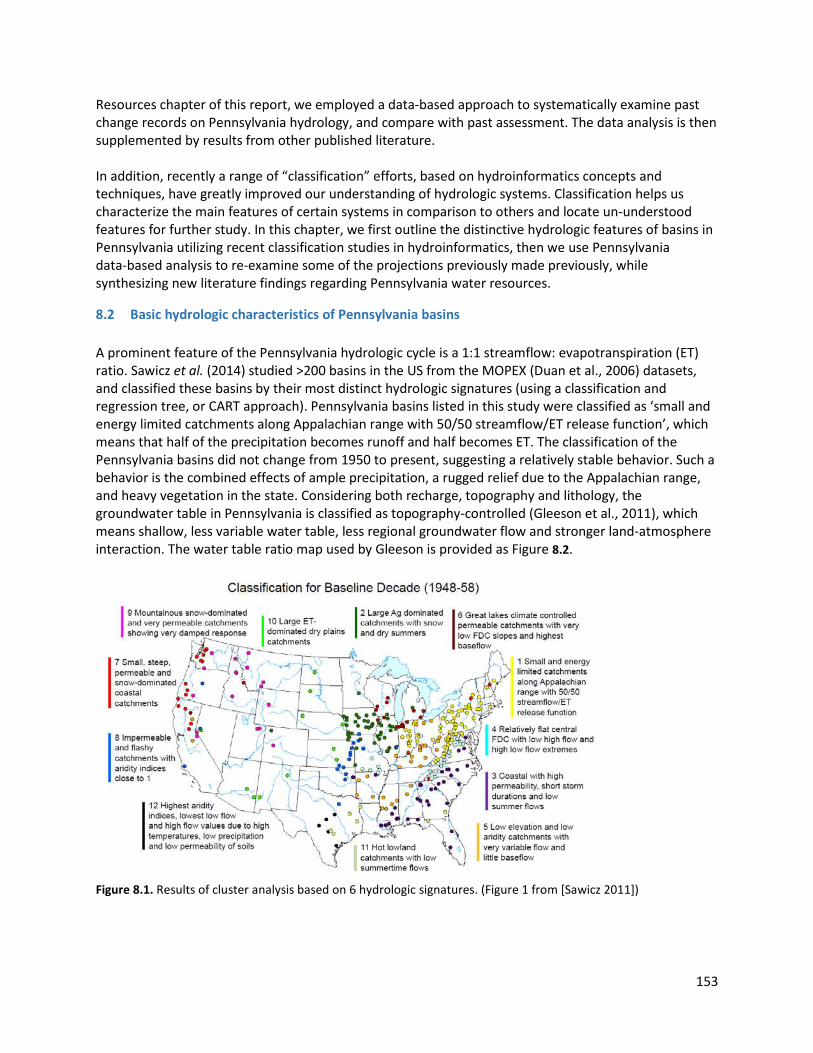
153

Resources chapter of this report, we employed a data-based approach to systematically examine past change records on Pennsylvania hydrology, and compare with past assessment. The data analysis is then supplemented by results from other published literature. In addition, recently a range of “classification” efforts, based on hydroinformatics concepts and techniques, have greatly improved our understanding of hydrologic systems. Classification helps us characterize the main features of certain systems in comparison to others and locate un-understood features for further study. In this chapter, we first outline the distinctive hydrologic features of basins in Pennsylvania utilizing recent classification studies in hydroinformatics, then we use Pennsylvania data-based analysis to re-examine some of the projections previously made previously, while synthesizing new literature findings regarding Pennsylvania water resources.

8.2 Basic hydrologic characteristics of Pennsylvania basins A prominent feature of the Pennsylvania hydrologic cycle is a 1:1 streamflow: evapotranspiration (ET) ratio. Sawicz et al. (2014) studied >200 basins in the US from the MOPEX (Duan et al., 2006) datasets, and classified these basins by their most distinct hydrologic signatures (using a classification and regression tree, or CART approach). Pennsylvania basins listed in this study were classified as ‘small and energy limited catchments along Appalachian range with 50/50 streamflow/ET release function’, which means that half of the precipitation becomes runoff and half becomes ET. The classification of the Pennsylvania basins did not change from 1950 to present, suggesting a relatively stable behavior. Such a behavior is the combined effects of ample precipitation, a rugged relief due to the Appalachian range, and heavy vegetation in the state. Considering both recharge, topography and lithology, the groundwater table in Pennsylvania is classified as topography-controlled (Gleeson et al., 2011), which means shallow, less variable water table, less regional groundwater flow and stronger land-atmosphere interaction. The water table ratio map used by Gleeson is provided as Figure 8.2.

Figure 8.1. Results of cluster analysis based on 6 hydrologic signatures. (Figure 1 from [Sawicz 2011])

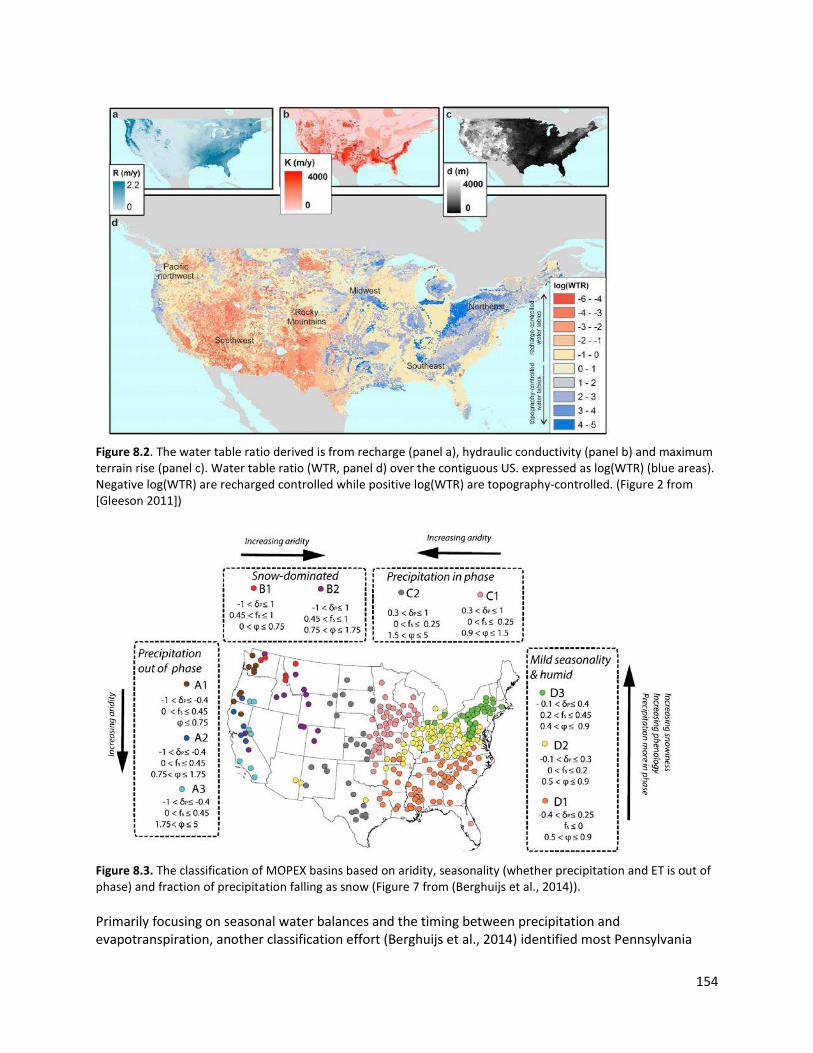
154

Figure 8.2. The water table ratio derived is from recharge (panel a), hydraulic conductivity (panel b) and maximum terrain rise (panel c). Water table ratio (WTR, panel d) over the contiguous US. expressed as log(WTR) (blue areas). Negative log(WTR) are recharged controlled while positive log(WTR) are topography-controlled. (Figure 2 from [Gleeson 2011])

Figure 8.3. The classification of MOPEX basins based on aridity, seasonality (whether precipitation and ET is out of phase) and fraction of precipitation falling as snow (Figure 7 from (Berghuijs et al., 2014)). Primarily focusing on seasonal water balances and the timing between precipitation and evapotranspiration, another classification effort (Berghuijs et al., 2014) identified most Pennsylvania

155

catchments as D3: humid with mild seasonality (precipitation and ET are slightly in phase), also using the MOPEX dataset. Using the above understanding, we can place some first-order estimate of how Pennsylvania water balance is likely to shift as a result of climate change in precipitation: ET is expected to increase in proportion to increase in precipitation. As total precipitation is expected to increase and snow fraction is decreasing, we expect more winter runoff and the catchment exhibiting more flow variability.

8.3 Data-based assessment of climate change impacts in the past decade This chapter of the report includes analysis of the following data products to give a comprehensive view of the changes in the hydrologic cycle in the past decade:

1. Terrestrial water storage anomalies from GRACE (2002-2013) 2. USGS streamflow records (1974-2014) 3. USGS groundwater records from the climate change response network 4. USGS stream temperature records 5. Soil moisture fields from the North American Land Data Assimilation System (NLDAS)

Due to the lack of data, we synthesize literature studies on river bed elevation and bank erosion.

8.3.1 Terrestrial water storage anomalies from GRACE (2002-2013) The GRACE satellite mission (http://www.nasa.gov/mission_pages/Grace/) allows unprecedented observation of global-scale water storage trends. The twin satellites were launched in mid-2002 and have since been lauded as a scientific triumph. GRACE data has been used to detect groundwater depletion in the US (California and Texas) (Famiglietti et al., 2011; Scanlon et al., 2012), China (Feng et al., 2013), India (Chen et al., 2014), Arabic peninsula (Voss et al., 2013), and other parts of the world (Döll et al., 2014), monitor mass loss in arctic glaciers (Gardner et al., 2011), identify basin hydrologic behavior (Reager and Famiglietti, 2013), infer flooding potential (Reager and Famiglietti, 2009; Reager et al., 2014) and identify decadal water storage changes after mega-drought (Chen et al., 2010; Wang et al., 2012). The mission consists of an array of two satellites making detailed measurements of the Earth’s gravity fields, whose tiny changes are mostly attributed to changes in the total amounts of water in all forms of storages on land (JPL, 2014; Landerer and Swenson, 2012; Swenson and Wahr, 2006), including groundwater, soil moisture, snow, streams and surface reservoirs. GRACE data products are provided as terrestrial water storage anomalies (TWSA). Simply put, imagine all water on land is evenly distributed as a thin layer mantling Earth’s surface, the deviation of the thickness of the water layer from its long-term average is the TWSA, in cm (1 cm = 0.393 inch). Therefore GRACE data reflect the changes of the total mass stored on land, which should be correlated with storages in different compartments. Over the long-term, groundwater and, less so, soil moisture, are the main components whose changes contribute to the changes in TWSA. GRACE data is limited by spatial and temporal resolution, with TWSA provided at 1 latitude-longitude degree resolution and monthly intervals. Extensive post-processing steps are involved to extract the TWSA data presented here, in equivalent water thickness in cm. The state of Pennsylvania intersects with 21 GRACE cells. For reader’s convenience, a latitude-longitude map, whose boxes correspond to GRACE cells, has been provided in Figure 8A.1 in the appendix. The time series of 8 of these cells are provided in Figure 8.4. We estimated the long-term average change rate (Mann-Kendall tau-b test with Sen’s method), and the trend lines have also been shown in the

156

Figure. In summary, TWSA in Pennsylvania show a large seasonal variation but overall small inter-annual trends. The average peak-to-trough variation of the TWSA can be from 10cm to -10cm (3.9in to-3.9in). Trend analysis from 2003 to 2013 of TWSA over the state shows a small positive trend in the state, with generally higher change rate in the northeast direction (Figure 8.5). Only two southwestern pixels (surrounding Pittsburgh) showed a small negative trend. To put Pennsylvania into a national context, Pennsylvania’s seasonal variation is relatively large, mainly due to higher precipitation, compared to more western states. Storage trend from 2003 to 2012 was analyzed and presented in (Famiglietti and Rodell, 2013) and shown in Figure 8.6. Pennsylvania is at the interface between a declining-storage center that extends northeast-ward from North Carolina and the rising-storage region in New York state. Compared to the small trend experienced by Pennsylvania, many other parts of the nation are undergoing significant changes: the central valley in CA, the Southern High Plains and eastern part of Texas, Alabama and the Mid-Atlantic states all show substantial storage decline (>2 cm/year, or 0.79 in/year). The Upper Missouri River basin (North, South Dakota and Nebraska) are experiencing a rising storage trend as the area is recovering from the extreme Canadian Prairies drought between 1999 and 2005 (Wang et al., 2012). In comparison, Pennsylvania underwent only mild long-term changes (maximum change is ~0.22 cm/year, or 0.08 in/year) and had a short memory of drought. We notice several large dips in the time series in Figure 8.4, in years 2002, 2007 and 2012, respectively, indicating relatively dry summers in these years. However, the TWSA fully recovered in the following years, suggesting a resilient terrestrial water storage system in Pennsylvania. This short storage memory is attributed to (a) the abundance of precipitation in most years; and (b) a topography-controlled groundwater table that prevents much over-year storage. In humid areas, higher storage often suggest higher flood potential (Reager et al., 2014) . The trending up storage in PA in the last decade suggested increasing risk of floods. However, because GRACE data is not available before April 2002, we cannot establish historical trend before 2002.

Figure 8.4. Sample time series of TWSA for 6 GRACE cells located in PA. Longitudes/latitudes have been provided in the title. These 1 degree by 1 degree cells, in the order of a-f, contain the following cities, respectively: Tionesta, Wellsboro, Scranton, Greensburg/Pittsburg, Lewistown and Allentown.

a b c

d e f

157

Figure 8.5. Change trends of GRACE TWSA and USGS groundwater CRN in PA from 2003 to 2014.

Figure 8.6. Change trend of TWSA of conterminous USA from 2003 to 2013 from (Famiglietti and Rodell, 2013)

8.3.2 Streamflow (1964-2014) In the past report, changes in runoff were expected to “overall increase, but mainly due to winter runoff. Decrease in summer runoff due to higher evapotranspiration” with moderate confidence. This was based on global scale analysis and similarity of Pennsylvania to Eastern U.S. from the 4th Annual IPCC

158

assessment, i.e., (Bates et al., 2008). Here we examine the trend in the past 5 decades using local datasets to provide a basis to evaluate future projections. We selected USGS streamflow stations in Pennsylvania that have more than 50 years of consecutive records (with more 95% data during 2004-2014 and more than 80% data during 1964-2014) and analyzed the change trends of flow distributions. 127 stations have been identified, which are shown in Figure 8.7. Out of the 127 streamflow stations we analyzed, 41 stations (32%) have seen the 50-year-largest (water years 1965-2014) event in the most recent decade, 2005-2014. This is significantly (P ≈ 0) higher frequency than would be from a stationary-in-time distribution (20%). While data is not shown, the trend is more obvious when compared to the previous decade (1995-2004): 93 stations (73%) have seen a higher event in the most recent decade than in 1995-2004. In fact, there are broad rises of streamflow across all flow regimes (Figure 8.8). Most rivers (~90% of the analyzed stations) show an increase in runoff in all percentile flows and only ~10% of the stations show small decreases. This is consistent with the descriptions in IPCC reports (Bates et al., 2008) and summarized in past Pennsylvania Climate Change impact assessment. However, on the high flow side, the increase of the 99 percentile flow (𝑄99, close to the annual 4-day high flow), the annually high flows that could potentially cause damage, is most significant: 10% of the stations show a 30% higher annual 𝑄99, 27% of the stations show a 20% higher 𝑄99, and 56% stations show a 10% higher 𝑄99 (Figure 8.8a). On the low flow side, most stations also observed a higher flow during low flow periods. For example, for 2 percentile flow (𝑄2 , close to annual 7-day low flow) Figure 8.8b shows that for 9% of the stations, there are large increases (more than 100%) in 𝑄2 , 20% stations saw more than 56% increase in 𝑄2 , 80% saw more than 10% increase in 𝑄2 and only 7 stations, or 5.5%, observed a decrease in 𝑄2 , although these decreases can be substantial in percentage (see insert in Figure 8.8b). In these few streams, the decrease (up to -30% change in 𝑄2 ) can have adverse impacts on stream ecology. The increases in low flows are suspected to be due to higher subsurface water storage and sustained baseflow that gradually releases during the year. To see how the changes are correlated with stream order and streamflow variability, we show the scatter plot of median flow (2005-2014), 𝑄99 percentage change from 1965-2004 and slope of the flow duration curve (SFDC) in Figure 8.9. SFDC is the slope between the 66% and 33% flow exceedance percentiles, and characterizes flow variability (Yadav et al., 2007; Zhang et al., 2008). Streams with low SFDC are expected to be dominated by relatively constant input such as baseflow. As we can see, most stations that underwent >20% 𝑄99 changes are small-to-medium streams with annual median flow between 1 to 20 m3/s (706 cfs), especially streams with low SFDC. This suggests smaller, low-variability streams, typically dominated by baseflow, now see more flash flows. 𝑄99 changes experienced by high-variability streams, shows as orange-yellow colored dots in the figure, are mostly between -5% to 20%, except for the two smallest, quick-flow dominated streams that have an annual median flow of less than 0.2 m3/s. Their peaks have become more flashy. The stations measuring the largest flows, located near the right end of the scatter plot, typically have an intermediate SFDC of ~1.2. The flow variability is damped as large basins averages out pulses from tributaries. 𝑄99 of these stations with largest flows have increased 5-20% compared to 1965-2004. Figure 8.7 also shows the map of 𝑄99 percent changes in the past decade compared to water years 1995-2004. There is a discernible spatial pattern in 𝑄99 percent change. The southwest quadrant, except for the Pittsburg area, observed many more streams with decreasing 𝑄99 than rest of the state, which experienced significant rise of annual 1% high flows.

159

In summary, the recent change trends strongly support previous predictions of higher flooding potential in the state due to higher precipitation. As was suggested, the extreme flows have become more extreme in much of the state except for the south-west quadrant, where some lower high flows were observed. The changes in high flow volumes are most substantial (>20%) with some small to medium streams, while the largest streams saw moderate (5-20%) increases. However, except for a few streams, we did not notice lower streamflow in summer and fall. Instead most low flow discharges increased as well. As climate models predicted higher precipitation in the coming decades, the flooding risks is expected to continue to rise. Although dry periods are projected to be longer, its impacts should be evaluated using physically-based hydrologic models that better describes groundwater flow.

Figure 8.7. Map of selected USGS gages for streamflow and stream temperature analysis. Stream temperature gages have been labeled.

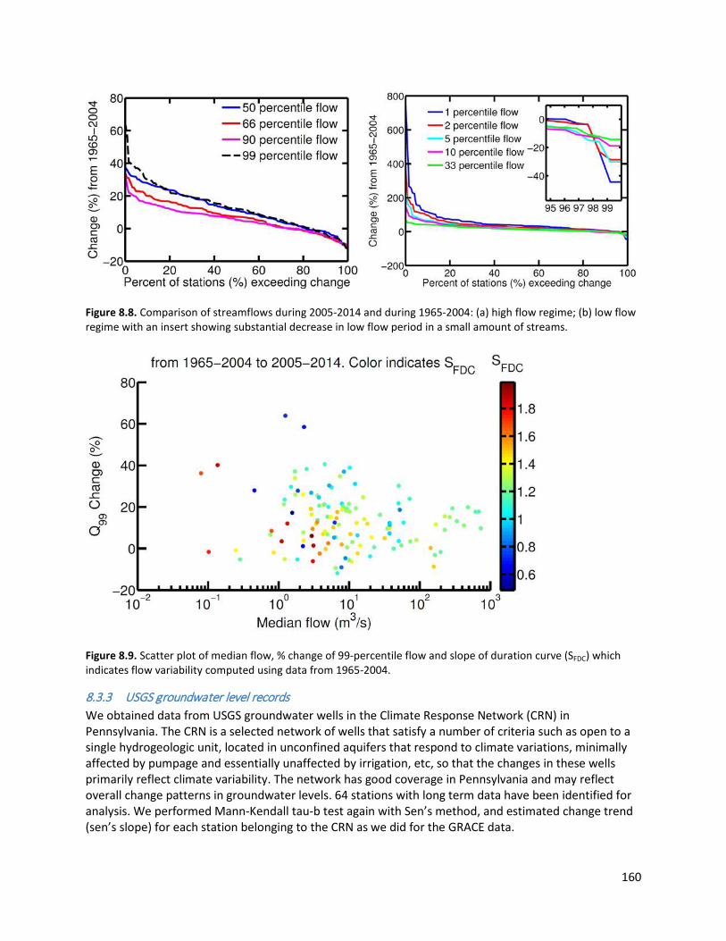
160

Figure 8.8. Comparison of streamflows during 2005-2014 and during 1965-2004: (a) high flow regime; (b) low flow regime with an insert showing substantial decrease in low flow period in a small amount of streams.

Figure 8.9. Scatter plot of median flow, % change of 99-percentile flow and slope of duration curve (SFDC) which indicates flow variability computed using data from 1965-2004.

8.3.3 USGS groundwater level records We obtained data from USGS groundwater wells in the Climate Response Network (CRN) in Pennsylvania. The CRN is a selected network of wells that satisfy a number of criteria such as open to a single hydrogeologic unit, located in unconfined aquifers that respond to climate variations, minimally affected by pumpage and essentially unaffected by irrigation, etc, so that the changes in these wells primarily reflect climate variability. The network has good coverage in Pennsylvania and may reflect overall change patterns in groundwater levels. 64 stations with long term data have been identified for analysis. We performed Mann-Kendall tau-b test again with Sen’s method, and estimated change trend (sen’s slope) for each station belonging to the CRN as we did for the GRACE data.

161

The change trends based on USGS CRN data has been shown in Figure 8.5, together with the GRACE TWSA change trend. The histogram of the 64 stations is provided in Figure 8.11. The state-averaged CRN trend generally agrees with the mildly increasing trend from GRACE. However, the spatial trend of the CRN data is not in good agreement with TWSA. GRACE shows an overall higher rising trend in the Northern half while the CRN data produces mixed trends. Some wells in the northern half showed small declining trends. There is no discernible spatial pattern from the CRN data. Many researchers have found it difficult to link GRACE data with well observations, and some discrepancy is to be expected. Many local factors such as topography, location of the wells on the slope, and local geologic complexity contribute to the different responses of the wells. Especially, as the groundwater dynamics in Pennsylvania is topography-controlled (Figure 8.2), groundwater head gradient can be significant at local hillslope scale. This means that influence on local hydrology needs to be examined using more detailed, physically-based models that resolve local flow processes.

Figure 8.10. Examples of changes in the flow duration curve during the past five decades. To highlight the high flows, the x-axis is shown on the log scale.

162

Figure 8.11. Histogram of the groundwater level change trends from USGS Climate Response Network, based on data from 2003 to 20148.0.1 Stream temperature trends (1994-2014)

8.3.4 USGS stream temperature In 2013 report, the change trend of PA stream temperature was“increase in stream temperature for most streams likely. Some spring fed headwater streams less affected” with high confidence. This was based on analysis of correlation between stream temperature and air temperature. This is indeed a conclusion we confirmed in our analysis here. However the analysis did not include winter stream temperature. We identified USGS gages with sufficient stream temperature records to establish trends from the 1990 to current and with more than 8 years of data in the most recent decade, resulting in only 15 gages in the state. We removed years that have less than 85% valid entries from the analysis. The gage IDs and gage names are provided in Table 8A.1. Due to the paucity of data, our analysis is just for reference and does not provide an adequate picture of the state-wide stream temperature trends. Table 8.2 shows the results for the 15 selected USGS gages whose locations are shown in Figure 8.7. Some of these gages have data only in the summer time so only mean summer-time (June 15th- August 15th) change trend (𝑠𝑠𝑠𝑠𝑠𝑠𝑠

𝑦𝑠𝑦𝑠𝑦𝑦 ) was possible. The data showed a mixed message. 6 stations, three of which are on the Brandywine Creek, showed apparent cooling trends (𝑠𝑠𝑠𝑠𝑠𝑠𝑠

𝑦𝑠𝑦𝑠𝑦𝑦 < −0.01) during the hot season. Among these 6 stations, 3 are likely Spring-fed headwater streams, but the other 3 have relatively large catchment areas and unlikely to be dominated by baseflow. Two stations on the Delaware River showed a very small negative trend. The rest of the stations experienced apparent rising summer-time temperature. 5 stations (1427207, 1460200, 1480617, 1480870 and 1481000) saw lower 7-day and 15-day annual high temperatures (𝑇98ℎ > 𝑇98 and 𝑇96ℎ > 𝑇96), but the differences between historical and most-recent decade values are quite minor. 7 stations, on the other hand, saw increases in the hottest temperatures (𝑇98ℎ < 𝑇98 and 𝑇96ℎ < 𝑇96) which are more substantial. Especially, hot-season temperatures have become significantly hotter in the upstream and midstream Delaware River. Among the 12 stations with whole year record, many showed elongation of the hottest days (7 stations with 𝐷7𝑑ℎ > 7 and 8 with 𝐷15𝑑ℎ > 15) which could have negative impact on salmon population.

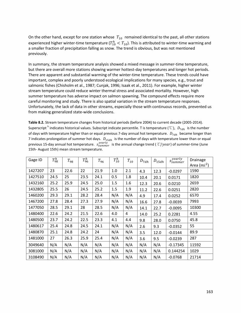
163

On the other hand, except for one station whose 𝑇10 remained identical to the past, all other stations experienced higher winter-time temperature (𝑇10ℎ < 𝑇10). This is attributed to winter-time warming and a smaller fraction of precipitation falling as snow. The trend is obvious, but was not mentioned previously. In summary, the stream temperature analysis showed a mixed message in summer-time temperature, but there are overall more stations showing warmer hottest-day temperatures and longer hot periods. There are apparent and substantial warming of the winter-time temperature. These trends could have important, complex and poorly understood ecological implications for many species, e.g., trout and salmonic fishes (Chisholm et al., 1987; Cunjak, 1996; Isaak et al., 2011). For example, higher winter stream temperature could reduce winter thermal stress and associated mortality. However, high summer temperature has adverse impact on salmon spawning. The compound effects require more careful monitoring and study. There is also spatial variation in the stream temperature responses. Unfortunately, the lack of data in other streams, especially those with continuous records, prevented us from making generalized state-wide conclusions. Table 8.2. Stream temperature changes from historical periods (before 2004) to current decade (2005-2014). Superscript h indicates historical values. Subscript indicate percentile. T is temperature (℃), 𝐷7𝑑ℎ is the number of days with temperature higher than or equal previous 7-day annual hot temperature. 𝐷7𝑑ℎ became longer than 7 indicates prolongation of summer hot days. 𝐷15𝑑ℎ is the number of days with temperature lower than or equal previous 15-day annual hot temperature. 𝑠𝑠𝑠𝑠𝑠𝑠𝑠

𝑦𝑠𝑦𝑠𝑦𝑦 is the annual change trend (℃/𝑦𝑒𝑦𝑦) of summer-time (June 15th- August 15th) mean stream temperature. Gage ID 𝑇98ℎ 𝑇98 𝑇96ℎ 𝑇96 𝑇10ℎ 𝑇10 𝐷7𝑑ℎ 𝐷15𝑑ℎ 𝑠𝑠𝑠𝑠𝑠𝑠𝑠

𝑦𝑠𝑦𝑠𝑦𝑦 Drainage Area (𝑚𝑚2)

1427207 23 22.6 22 21.9 1.0 2.1 4.3 12.3 -0.0297 1590 1427510 24.5 25 23.5 24.1 0.5 1.8 10.4 20.1 0.0171 1820 1432160 25.2 25.9 24.5 25.0 1.5 1.6 12.3 20.6 0.0210 2659 1432805 25.5 26 24.5 25.2 1.5 1.9 11.2 22.6 0.0251 2820 1460200 29.3 29.1 28.2 28.4 N/A N/A 4.9 17.4 0.0252 6570 1467200 27.8 28.4 27.3 27.9 N/A N/A 16.6 27.8 -0.0039 7993 1477050 28.5 29.1 28 28.5 N/A N/A 14.1 22.7 -0.0095 10300 1480400 22.6 24.2 21.5 22.6 4.0 4 14.0 25.2 0.2281 4.55 1480500 23.7 24.2 22.5 23.3 4.1 4.4 9.8 28.0 0.0750 45.8 1480617 25.4 24.8 24.5 24.1 N/A N/A 2.6 9.3 -0.0352 55 1480870 25.1 24.8 24.2 24 N/A N/A 3.5 12.0 -0.0144 89.9 1481000 27 26.3 25.9 25.4 N/A N/A 3.6 9.5 -0.0239 287 3049640 N/A N/A N/A N/A N/A N/A N/A N/A -0.17345 11592 3081000 N/A N/A N/A N/A N/A N/A N/A N/A 0.144254 1029 3108490 N/A N/A N/A N/A N/A N/A N/A N/A -0.0768 21714

164

8.3.5 Simulated soil moisture change (2004-2014) In-situ soil moisture measurements tend to be scattered in space and time and unable to support conclusions about state-wide trends in soil moisture. Instead we have employed simulated datasets from the North American Land Data Assimilation System (NLDAS) (http://ldas.gsfc.nasa.gov/nldas/). We used the Noah-LSM model for the results in this section. NLDAS simulations have been validated extensively (Xia et al., 2012) and therefore its simulated soil moisture should be considered reasonable. Figure 8.13. shows change trends of monthly mean top 1m soil moisture for the months of April, June and August in the past decade. In April, the northern half of the state shows some drying over the past decade, with a maximum trend of -0.2 cm/year, approximately 0.5% per year change from 2004. Over a period of 10 years this amounted to a 5% difference. There are some wetting trends along the Appalachian Mountains, with a maximum annual trend of 0.25 cm/year. Rest of the state stayed stationary. The entire state showed small increases in moisture in June, with the magnitude less than 0.156 cm/year. In August, most of the state shows a mild wetting (0.02-0.1 cm/year) while pockets of land, e.g., an area near McConnellsburg, showed some drying.

Figure 8.12. Sample temperature exceedance curves In summary, soil moisture changes are relatively minor, staying within a range of 5% change over the last decade. Some parts of the northern half of the state saw a drying trend in April most other areas experienced mild wetting in the last 10 years, consistently with the GRACE observations. Wetter soil on the mountain ranges could contribute to flash flood in spring during storms that coincide with snowmelt.

165

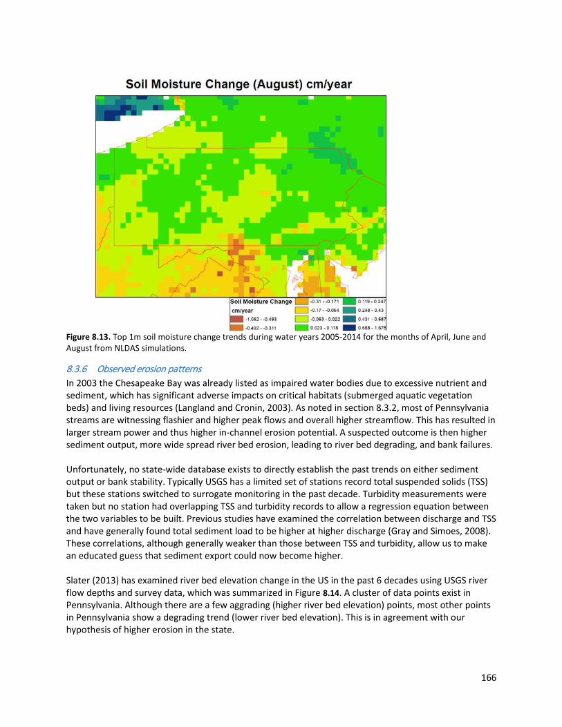
166

Figure 8.13. Top 1m soil moisture change trends during water years 2005-2014 for the months of April, June and August from NLDAS simulations.

8.3.6 Observed erosion patterns In 2003 the Chesapeake Bay was already listed as impaired water bodies due to excessive nutrient and sediment, which has significant adverse impacts on critical habitats (submerged aquatic vegetation beds) and living resources (Langland and Cronin, 2003). As noted in section 8.3.2, most of Pennsylvania streams are witnessing flashier and higher peak flows and overall higher streamflow. This has resulted in larger stream power and thus higher in-channel erosion potential. A suspected outcome is then higher sediment output, more wide spread river bed erosion, leading to river bed degrading, and bank failures. Unfortunately, no state-wide database exists to directly establish the past trends on either sediment output or bank stability. Typically USGS has a limited set of stations record total suspended solids (TSS) but these stations switched to surrogate monitoring in the past decade. Turbidity measurements were taken but no station had overlapping TSS and turbidity records to allow a regression equation between the two variables to be built. Previous studies have examined the correlation between discharge and TSS and have generally found total sediment load to be higher at higher discharge (Gray and Simoes, 2008). These correlations, although generally weaker than those between TSS and turbidity, allow us to make an educated guess that sediment export could now become higher. Slater (2013) has examined river bed elevation change in the US in the past 6 decades using USGS river flow depths and survey data, which was summarized in Figure 8.14. A cluster of data points exist in Pennsylvania. Although there are a few aggrading (higher river bed elevation) points, most other points in Pennsylvania show a degrading trend (lower river bed elevation). This is in agreement with our hypothesis of higher erosion in the state.

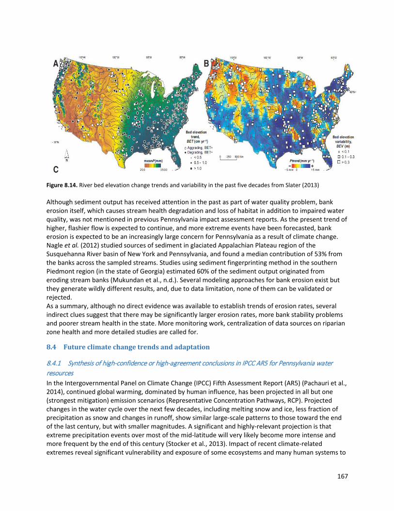
167

Figure 8.14. River bed elevation change trends and variability in the past five decades from Slater (2013) Although sediment output has received attention in the past as part of water quality problem, bank erosion itself, which causes stream health degradation and loss of habitat in addition to impaired water quality, was not mentioned in previous Pennsylvania impact assessment reports. As the present trend of higher, flashier flow is expected to continue, and more extreme events have been forecasted, bank erosion is expected to be an increasingly large concern for Pennsylvania as a result of climate change. Nagle et al. (2012) studied sources of sediment in glaciated Appalachian Plateau region of the Susquehanna River basin of New York and Pennsylvania, and found a median contribution of 53% from the banks across the sampled streams. Studies using sediment fingerprinting method in the southern Piedmont region (in the state of Georgia) estimated 60% of the sediment output originated from eroding stream banks (Mukundan et al., n.d.). Several modeling approaches for bank erosion exist but they generate wildly different results, and, due to data limitation, none of them can be validated or rejected. As a summary, although no direct evidence was available to establish trends of erosion rates, several indirect clues suggest that there may be significantly larger erosion rates, more bank stability problems and poorer stream health in the state. More monitoring work, centralization of data sources on riparian zone health and more detailed studies are called for.

8.4 Future climate change trends and adaptation

8.4.1 Synthesis of high-confidence or high-agreement conclusions in IPCC AR5 for Pennsylvania water resources In the Intergovernmental Panel on Climate Change (IPCC) Fifth Assessment Report (AR5) (Pachauri et al., 2014), continued global warming, dominated by human influence, has been projected in all but one (strongest mitigation) emission scenarios (Representative Concentration Pathways, RCP). Projected changes in the water cycle over the next few decades, including melting snow and ice, less fraction of precipitation as snow and changes in runoff, show similar large-scale patterns to those toward the end of the last century, but with smaller magnitudes. A significant and highly-relevant projection is that extreme precipitation events over most of the mid-latitude will very likely become more intense and more frequent by the end of this century (Stocker et al., 2013). Impact of recent climate-related extremes reveal significant vulnerability and exposure of some ecosystems and many human systems to

168

climate variability, consistent with a significant lack of preparedness for climate-related extremes. Climate change is projected to increase risks for people, assets, economies and ecosystems in urban areas, including risks from extreme precipitation, flooding and storm surges, while increase water availability issues in rural areas. Climate change will amplify risks to water resources already affected by non-climatic stressors, with potential impacts associated with decreased snowpack, decreased water quality, urban flooding, and decreased water supplies for urban areas and irrigation. Climate change is projected to reduce raw water quality and pose risks to drinking water quality even with conventional treatment, due to interacting factors: increased temperature; increased sediment, nutrient, and pollutant loadings from heavy rainfall; increased concentration of pollutants during droughts; and disruption of treatment facilities during floods. As flow and thermal regime in streams change, so will aquatic species and habitat. (Field et al., 2014) Adaptation planning and implementation, both place- and context-specific processes, can be enhanced through complementary actions across levels, from individuals to governments. Effective adaption and risk reduction strategies consider vulnerability, exposure and equity. Adaptation and mitigation in the near term can substantially reduce the impacts in the latter decades in the century. A first step toward adaptation is reducing vulnerability and exposure to present climate variability. Significant co-benefits, synergies and trade-offs exist between mitigation and adaptation and among different adaptation responses, while poor planning, especially those resulting from over-emphasizing short-term outcomes, can lead to maladaptation. Opportunities to take advantage of positive synergies between adaptation and mitigation may decrease with time. Transformations in economic, social, technological, and political decisions and actions can enable climate-resilient pathways (Field et al., 2014).

8.4.2 Adaptation suggestions for Pennsylvania water resources Combining the findings from our data-based studies and IPCC reports, we make the following statements regarding climate change impacts and adaptation for Pennsylvania water resources, in addition to the actions recommended in the last impact update: 1. ‘Low-regret’ adaptation methods that reduces vulnerability and exposure to present climate

variability with co-benefits, are preferred methods to create resilience under uncertain hydrological changes. Examples of these strategies include less impervious surfaces, green infrastructure, rooftop gardens and conservation of wetlands.

2. The impacts of droughts are likely to be short-term in Pennsylvania. However there are risks associated with short-term disasters, e.g., wetlands degradation and competition for water resources in low-flow, high-temperature periods between different sectors. Water availability issues for vulnerable communities may exist for due to multidimensional inequalities.

3. There are substantial and increasing flooding risks in Pennsylvania for both urban areas and infrastructure in rural areas. Adaptation strategies that focus on increasing flood preparedness, reducing vulnerabilities and increasing resilience in more extreme and more frequent flooding scenarios are of high priority. It is important to consider differential risks and vulnerabilities in adaptation strategies.

4. The state should initiate programs for monitoring, assessing, estimating and abating stream bank erosion (see Information Needs section) from not only water quality but also stream health standpoints.

169

8.5 Information needs New data collection effort should first examine multi-agency coordination, existing datasets and available remotely-sensed data products. However, some state-level effort will facilitate better hydrologic analysis. Below is a list of such potential datasets. Floods are localized, short-term features that may not be adequately captured by streamflow gages. Complete descriptions of past floods, including causes, extent, discharge, etc, in addition to conventionally available flooding risk map, can be of great value in future forecasting. There are also some nation-level efforts (e.g., http://pubs.er.usgs.gov/publication/70048422, http://www.dartmouth.edu/~floods/), which are somewhat limited in temporal coverage. Colorado has established their flood database (Kohn, 2014). As Pennsylvania basins are characterized by small basin sizes, rugged relief and a topography-controlled water table, groundwater changes are more strongly controlled by local processes instead of large-scale trends, as we have shown in the trends between GRACE and USGS CRN data. Physically-based, integrated hydrologic modeling may better resolve the local hydrologic processes and help better predict changes in groundwater resources. To apply physically-based hydrologic models, however, geologic inputs such as soil thickness and aquifer thickness and conductivity is required. There is no state-wide hydrogeologic database that details these attributes, especially vertical stratigraphic information. A stronger monitoring program for sediment sources and bank retreat is encouraged. Currently data regarding existing bank erosion rates is critically lacking. Lots of survey data may exist as proprietary holdings of contractors. However, they are decentralized and inaccessible. The effort may start from collecting and compiling existing survey data from previous stream restoration projects, and set forth better data sharing policies for future projects. More systematic estimates of contributions of sediment output from bank material will be helpful.

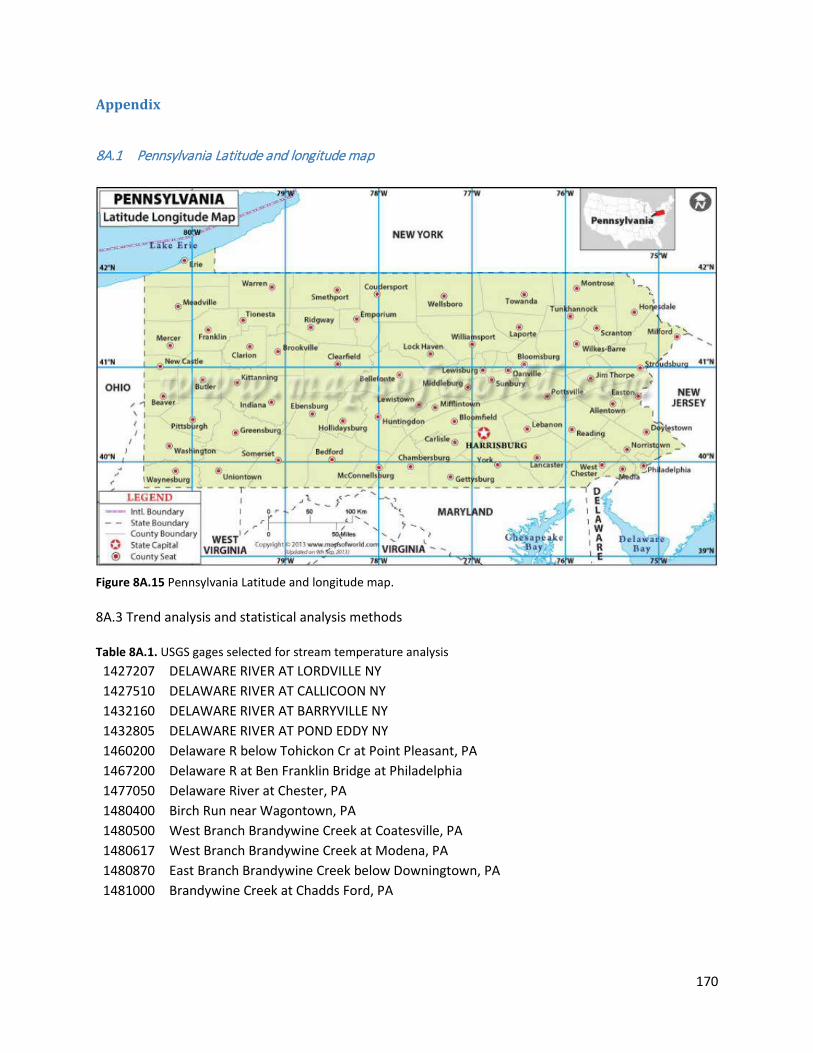
170

Appendix

8A.1 Pennsylvania Latitude and longitude map

Figure 8A.15 Pennsylvania Latitude and longitude map. 8A.3 Trend analysis and statistical analysis methods Table 8A.1. USGS gages selected for stream temperature analysis

1427207 DELAWARE RIVER AT LORDVILLE NY 1427510 DELAWARE RIVER AT CALLICOON NY 1432160 DELAWARE RIVER AT BARRYVILLE NY 1432805 DELAWARE RIVER AT POND EDDY NY 1460200 Delaware R below Tohickon Cr at Point Pleasant, PA 1467200 Delaware R at Ben Franklin Bridge at Philadelphia 1477050 Delaware River at Chester, PA 1480400 Birch Run near Wagontown, PA 1480500 West Branch Brandywine Creek at Coatesville, PA 1480617 West Branch Brandywine Creek at Modena, PA 1480870 East Branch Brandywine Creek below Downingtown, PA 1481000 Brandywine Creek at Chadds Ford, PA

171

References Bates, B. C., Kundzewicz, Z. W., Wu, S. and Palutikof, J. P.: Climate Change and Water, IPCC Technical

Paper VI., Intergovernmental Panel on Climate Change, Geneva., 2008. Berghuijs, W. R., Sivapalan, M., Woods, R. A. and Savenije, H. H. G.: Patterns of similarity of seasonal

water balances: A window into streamflow variability over a range of time scales, Water Resource. Res., 50(7), 5638–5661, doi:10.1002/2014WR015692, 2014.

Chen, J. L., Wilson, C. R. and Tapley, B. D.: The 2009 exceptional Amazon flood and interannual terrestrial water storage change observed by GRACE, Water Resource. Res., 46(12), doi:10.1029/2010WR009383, 2010.

Chen, J., Li, J., Zhang, Z. and Ni, S.: Long-term groundwater variations in Northwest India from satellite gravity measurements, Glob. Planet. Change, 116, 130–138, doi:10.1016/j.gloplacha.2014.02.007, 2014.

Chisholm, I. M., Hubert, W. A. and Wesche, T. A.: Winter Stream Conditions and Use of Habitat by Brook Trout in High-Elevation Wyoming Streams, Trans. Am. Fish. Soc., 116(2), 176–184, doi:10.1577/1548-8659(1987)116<176:WSCAUO>2.0.CO;2, 1987.

Cunjak, R. A.: Winter habitat of selected stream fishes and potential impacts from land-use activity, Can. J. Fish. Aquat. Sci., 53(S1), 267–282, doi:10.1139/f95-275, 1996.

Döll, P., Fritsche, M., Eicker, A. and Müller Schmied, H.: Seasonal Water Storage Variations as Impacted by Water Abstractions: Comparing the Output of a Global Hydrological Model with GRACE and GPS Observations, Surv. Geophys., doi:10.1007/s10712-014-9282-2, 2014.

Duan, Q., Schaake, J., Andréassian, V., Franks, S., Goteti, G., Gupta, H. V., Gusev, Y. M., Habets, F., Hall, A., Hay, L., Hogue, T., Huang, M., Leavesley, G., Liang, X., Nasonova, O. N., Noilhan, J., Oudin, L., Sorooshian, S., Wagener, T. and Wood, E. F.: Model Parameter Estimation Experiment (MOPEX): An overview of science strategy and major results from the second and third workshops, J. Hydrol., 320(1-2), 3–17, doi:10.1016/j.jhydrol.2005.07.031, 2006.

Famiglietti, J. S., Lo, M., Ho, S. L., Bethune, J., Anderson, K. J., Syed, T. H., Swenson, S. C., de Linage, C. R. and Rodell, M.: Satellites measure recent rates of groundwater depletion in California’s Central Valley, Geophys. Res. Lett., 38(3), n/a–n/a, doi:10.1029/2010GL046442, 2011.

Famiglietti, J. S. and Rodell, M.: Water in the balance., Science (80-. )., 340(6138), 1300–1, doi:10.1126/science.1236460, 2013.

Feng, W., Zhong, M., Lemoine, J.-M., Biancale, R., Hsu, H.-T. and Xia, J.: Evaluation of groundwater depletion in North China using the Gravity Recovery and Climate Experiment (GRACE) data and ground-based measurements, Water Resour. Res., 49(4), 2110–2118, doi:10.1002/wrcr.20192, 2013.

Field, C. B., Barros, V. R., Mach, K. J., Mastrandrea, M. D., Aalst, M. van, Adger, W. N., Arent, D. J., Barnett, J., Betts, R., Bilir, T. E., Birkmann, J., Carmin, J., Chadee, D. D., Challinor, A. J., Chatterjee, M., Cramer, W., Davidson, D. J., Estrada, Y. O., Gattuso, J.-P., Hijioka, Y., Hoegh-Guldberg, O., Huang, H. Q., Insarov, G. E., Jones, R. N., Kovats, R. S., Romero-Lankao, P., Larsen, J. N., Losada, I. J., Marengo, J. A., McLean, R. F., Mearns, L. O., Mechler, R., Morton, J. F., Niang, I., Oki, T., Olwoch, J. M., Opondo, M., Poloczanska, E. S., Pörtner, H.-O., Redsteer, M. H., Reisinger, A., Revi, A., Schmidt, D. N., Shaw, M. R., Solecki, W., Stone, D. A., Stone, J. M. R., Strzepek, K. M., Suarez, A. G., Tschakert, P., Valentini, R., Vicuña, S., Villamizar, A., Vincent, K. E., Warren, R., White, L. L., Wilbanks, T. J., Wong, P. P. and Yohe, G. W.: Technical summary, in Climate Change 2014: Impacts, Adaptation, and Vulnerability. Part A: Global and Sectoral Aspects. Contribution of Working Group II to the Fifth Assessment Report of the Intergovernmental Panel on Climate Change, edited by C. B. Field, V. R. Barros, D. J. Dokken, K. J. Mach, M. D. Mastrandrea, T. E. Bilir, M. Chatterjee, K. L. Ebi, Y. O. Estrada, R. C. Genova, B. Girma, E. S. Kissel, A. N. Levy, S. MacCracken, P. R.

172

Mastrandrea, and L. L. White, Cambridge University Press, Cambridge, United Kingdom and New York, NY, USA., 2014.

Gardner, A. S., Moholdt, G., Wouters, B., Wolken, G. J., Burgess, D. O., Sharp, M. J., Cogley, J. G., Braun, C. and Labine, C.: Sharply increased mass loss from glaciers and ice caps in the Canadian Arctic Archipelago., Nature, 473(7347), 357–60, doi:10.1038/nature10089, 2011.

Gleeson, T., Marklund, L., Smith, L. and Manning, A. H.: Classifying the water table at regional to continental scales, Geophys. Res. Lett., 38(5), doi:10.1029/2010GL046427, 2011.

Gray, J. R. and Simoes, F. J. M.: Estimating sediment discharge, in Sedimentation Engineering: Processes, Measurements, Modeling, and Practice, pp. 1057–1088. [online] Available from: http://www.jlakes.org/web/wrir00-4191.pdf, 2008.

Isaak, D. J., Wollrab, S., Horan, D. and Chandler, G.: Climate change effects on stream and river temperatures across the northwest U.S. from 1980–2009 and implications for salmonid fishes, Clim. Change, 113(2), 499–524, doi:10.1007/s10584-011-0326-z, 2011.

JPL: GRACE monthly mass grids - land, Jet Propuls. Lab. GRACE Tellus, data Process. by Sean Swenson [online] Available from: http://grace.jpl.nasa.gov, 2014.

Kohn, M.: Colorado Flood Database, [online] Available from: http://co.water.usgs.gov/projects/COFloodDB/, 2014.

Landerer, F. W. and Swenson, S. C.: Accuracy of scaled GRACE terrestrial water storage estimates, Water Resource. Res., 48(4), n/a–n/a, doi:10.1029/2011WR011453, 2012.

Langland, M. and Cronin, T.: A Summary Report of Sediment Processes in Chesapeake Bay and Watershed., USGS Water-Resources Investig. Rep. 03-4123 [online] Available from: http://pa.water.usgs.gov/reports/wrir03-4123.pdf, 2003.

Mukundan, R., Radcliffe, D. E., Ritchie, J. C., Risse, L. M. and McKinley, R. A.: Sediment fingerprinting to determine the source of suspended sediment in a southern Piedmont stream, J. Environ. Qual., 39(4), 1328–37 [online] Available from: http://www.ncbi.nlm.nih.gov/pubmed/20830921 (Accessed 22 December 2014), n.d.

Nagle, G. N., Fahey, T. J., Woodbury, P. B. and Ritchie, J. C.: Bank Erosion in Fifteen Tributaries in the Glaciated Upper Susquehanna Basin of New York and Pennsylvania, Phys. Geogr., 33(3), 229–251, doi:10.2747/0272-3646.33.3.229, 2012.

Pachauri, R. K., Allen, M. R., Barros, V. R., Broome, J., Cramer, W., Christ, R., Church, J. A., Clarke, L., Dahe, Q., Dasgupta, P., Dubash, N. K., Edenhofer, O., Elgizouli, I., Field, C. B., Forster, P., Friedlingstein, P., Fuglestvedt, J., Gomez-Echeverri, L., Hallegatte, S., (United, G. H., Howden, M., Jiang, K., Cisneros, B. J., Kattsov, V., Lee, H., Mach, K. J., Marotzke, J., Mastrandrea, M. D., Meyer, L., Minx, J., Mulugetta, Y., O’Brien, K., Oppenheimer, M., Pereira, J. J., Pichs-Madruga, R., Plattner, G.-K., Pörtner, H.-O., Power, S. B., Preston, B., N.H., R., Reisinger, A., Riahi, K., Rusticucci, M., (South, R. S., Seyboth, K., Sokona, Y., Stavins, R., Stocker, T. F., Tschakert, P., Vuuren, D. van and Ypersele, J.-P. van: Summary for Policy Makers, Synth. Rep. Fifth Assess. Rep. Intergov. Panel Clim. Chang. [online] Available from: http://www.ipcc.ch/pdf/assessment-report/ar5/syr/SYR_AR5_SPMcorr1.pdf, 2014.

Reager, J. T. and Famiglietti, J. S.: Global terrestrial water storage capacity and flood potential using GRACE, Geophys. Res. Lett., 36(23), L23402, doi:10.1029/2009GL040826, 2009.

Reager, J. T. and Famiglietti, J. S.: Characteristic mega-basin water storage behavior using GRACE., Water Resour. Res., 49(6), 3314–3329, doi:10.1002/wrcr.20264, 2013.

Reager, J. T., Thomas, B. F. and Famiglietti, J. S.: River basin flood potential inferred using GRACE gravity observations at several months lead time, Nat. Geosci., 7(8), 588–592, doi:10.1038/ngeo2203, 2014.

173

Sawicz, K. A., Kelleher, C., Wagener, T., Troch, P., Sivapalan, M. and Carrillo, G.: Characterizing hydrologic change through catchment classification, Hydrol. Earth Syst. Sci., 18(1), 273–285, doi:10.5194/hess-18-273-2014, 2014.

Scanlon, B. R., Faunt, C. C., Longuevergne, L., Reedy, R. C., Alley, W. M., McGuire, V. L. and McMahon, P. B.: Groundwater depletion and sustainability of irrigation in the US High Plains and Central Valley., Proc. Natl. Acad. Sci. U. S. A., 109(24), 9320–5, doi:10.1073/pnas.1200311109, 2012.

Slater, L. J. and Singer, M. B.: Imprint of climate and climate change in alluvial riverbeds: Continental United States, 1950-2011, Geology, 41(5), 595–598, doi:10.1130/G34070.1, 2013.

Stocker, T. F., Qin, D., Plattner, G.-K., Alexander, L. V., Allen, S. K., Bindoff, N. L., Bréon, F.-M., Church, J. A., Cubasch, U., Emori, S., Forster, P., Friedlingstein, P., Gillett, N., Gregory, J. M., Hartmann, D. L., Jansen, E., Kirtman, B., Knutti, R., Kumar, K. K., Lemke, P., Marotzke, J., Masson-Delmotte, V., Meehl, G. A., Mokhov, I. I., Piao, S., Ramaswamy, V., Randall, D., Rhein, M., Rojas, M., Sabine, C., Shindell, D., Talley, L. D., Vaughan, D. G. and Xie, S.-P.: Technical summary, in Climate Change 2013: The Physical Science Basis. Contribution of Working Group I to the Fifth Assessment Report of the Intergovernmental Panel on Climate Change, edited by S. T.F., D. Qin, G.-K. Plattner, M. Tignor, S. K. Allen, J. Boschung, A. Nauels, Y. Xia, V. Bex, and P. M. Midgley, Cambridge University Press, Cambridge, United Kingdom and New York, NY, USA. [online] Available from: http://www.ipcc.ch/pdf/assessment-report/ar5/wg1/WG1AR5_TS_FINAL.pdf, 2013.

Swenson, S. and Wahr, J.: Post-processing removal of correlated errors in GRACE data, Geophys. Res. Lett., 33(8), L08402, doi:10.1029/2005GL025285, 2006.

Voss, K. A., Famiglietti, J. S., Lo, M., Linage, C., Rodell, M. and Swenson, S. C.: Groundwater depletion in the Middle East from GRACE with implications for transboundary water management in the Tigris-Euphrates-Western Iran region., Water Resour. Res., 49(2), 904–914, doi:10.1002/wrcr.20078, 2013.

Wang, H., Jia, L., Steffen, H., Wu, P., Jiang, L., Hsu, H., Xiang, L., Wang, Z. and Hu, B.: Increased water storage in North America and Scandinavia from GRACE gravity data, Nat. Geosci., 6(1), 38–42, doi:10.1038/ngeo1652, 2012.

Xia, Y., Mitchell, K., Ek, M., Sheffield, J., Cosgrove, B., Wood, E., Luo, L., Alonge, C., Wei, H., Meng, J., Livneh, B., Lettenmaier, D., Koren, V., Duan, Q., Mo, K., Fan, Y. and Mocko, D.: Continental-scale water and energy flux analysis and validation for the North American Land Data Assimilation System project phase 2 (NLDAS-2): 1. Intercomparison and application of model products, J. Geophys. Res., 117(D3), D03109, doi:10.1029/2011JD016048, 2012.

Yadav, M., Wagener, T. and Gupta, H.: Regionalization of constraints on expected watershed response behavior for improved predictions in ungauged basins, Adv. Water Resour., 30(8), 1756–1774 [online] Available from: http://www.sciencedirect.com/science/article/pii/S0309170807000140 (Accessed 18 November 2013), 2007.

Zhang, Z., Wagener, T., Reed, P. and Bhushan, R.: Reducing uncertainty in predictions in ungauged basins by combining hydrologic indices regionalization and multiobjective optimization, Water Resour. Res., 44(12), doi:10.1029/2008WR006833, 2008.

174

9 Wetlands

9.1 Introduction Aquatic resources of Pennsylvania are primarily freshwater, and are a significant natural resource. While precise inventory accounts do not agree, the Pennsylvania State Water Plan (2009) presents the following census:

• about 86,000 miles of streams • nearly 4000 lakes, reservoirs and ponds • about 80 trillion gallons of groundwater • over 404,000 acres of wetlands • 56 miles of coast along the Delaware Estuary and 64 miles along Lake Erie

While lakes, reservoirs, and ponds present significant and important habitat and resources, many of these features represent manmade impoundments in the Commonwealth where natural hydrology and the corresponding aquatic ecosystems have already been modified to meet either functional (e.g. irrigation, drinking water supply) or aesthetic requirements. Since they are actively managed for a specific purpose, we cannot assess their future functioning and do not include them here. The Commonwealth’s coastal systems, the potential impacts of climate change, and recommended management actions have been extensively covered in other studies, and can be found at: Partnership for the Delaware Estuary Inc. (Kreeger et al., 2010) and the Model Forest Policy Program (Beecher et al., 2013). We therefore direct this assessment to the aquatic resources represented by freshwater streams and wetlands that are the signature feature of the Commonwealth. These resources are intertwined and dependent upon one another for ecological integrity. For example, the trout population of a headwater stream is dependent upon wetland habitat along its edge. For that reason, we discuss the impacts of climate change on wetlands and headwater streams as a riparian ecosystem, and as representative of the majority of the aquatic ecosystems of the Commonwealth. Pennsylvania’s streams and rivers are classified into 124,181 segments by Pennsylvania Department of Environmental Protection and Department of Transportation (data from Pennsylvania Spatial Data Access, www.pasda.psu.edu, accessed 2012) and are second only to Alaska in total stream miles in any state. The largest area of stream miles can be found in Ridge and Valley eco-region (21,605 miles), Pittsburgh Low Plateau (14,588), and Allegheny High Plateau eco-region (16,526), as reported in (http://www.dcnr.state.pa.us/wlhabitat/aquatic/streams.aspx). Nationally, the United States has destroyed over half of its original wetlands throughout the past 200 years, leaving approximately 100 million acres, while Pennsylvania has lost an estimated two-thirds of its original wetland acreage. Estimates of the total amount of current wetland area in the Commonwealth vary; the State Water Plan references the 404,000 acres reported by the U.S. Fish and Wildlife Service. The National Wetland Inventory data, as reported by the Pennsylvania Game Commission (http://www.pgc.state.pa.us/pgc/cwp/view.asp?a=496&q=165868) reports a total of 729,535 wetland acres found in more than 160,000 wetlands across the state. These occur in two major categories: a total of 146,816 acres are defined as lacustrine (lakes and ponds primarily), and 410,009 acres are defined as palustrine habitat (marshes, etc.). An additional 643 acres of estuarine habitat are located in the southeastern region along the Delaware River. Most of Pennsylvania’s wetlands (97 percent) are palustrine (bogs, fens, swamps, shallow pools). Emergent wetlands (marshes,

175

meadows) and shrub swamps comprise 10-20 percent of state wetlands. Generally, natural wetlands are concentrated in northeast and northwestern counties, with more than 50 percent of the wetlands in the state occurring in these areas (Tiner 1990). This update on the potential impacts of climate change on these resources concentrates on the ecosystem services of water quality improvement and habitat, describes the vulnerability of these valuable services, and expands previous analyses by presenting modeled case studies of seven watersheds across the Commonwealth.

9.2 Definition and Description of Ecosystem Services Wetlands and streams are diverse and productive, and provide a number of tangible and intangible benefits to society and the environment. These goods and services are termed “ecosystem services”, and the realization that they are critical for human health and well-being (Millennium Ecosystem Assessment, 2005) has heightened the need for assessments that can estimate the level of service provided, detect the impact of human activities (including climate change) on these ecosystem services, and guide us to restoration of these services (Zedler, 2003). The MEA defines four types of ecosystem services, termed regulating, provisioning, cultural, and supporting, that are provided by, or derived from, wetlands and headwater streams (Table 9.1). Many of the ecosystem services most highly valued by society are the regulating ones, including water quality improvement and flood control; provisioning ones such as production of fish and game are also valuable and are more commonly recognized as

Table 9.1. Ecosystem services provided by wetlands, as per the Millennium Ecosystem Assessment

176

“habitat”. The freshwater wetlands of Pennsylvania represent critical areas of aquatic ecosystem function, serving as nursery areas, sources of dissolved organic carbon, critical habitat, and stabilizers of available nitrogen, atmospheric sulfur, carbon dioxide, and methane [Mitsch and Gosselink, 2000]. Regulating ecosystem services of primary interest are (1) water regulation and (2) water quality improvement, which are tightly coupled to the provisioning services (hereafter referred to as habitat). We concentrate on water quality improvement and habitat ecosystem services in this chapter. Wetlands remove excess nitrate and sediment in runoff and groundwater from upland sources, preventing eutrophication in lakes and rivers (Johnston 1990; Haycock and Pinay 1993; Gilliam 1994; Jordan et al. 2003). Wetlands are also important sources of carbon to streams and lakes. In one study, wetlands were found to have contributed 63% of the total organic carbon flux to streams (Dosskey and Bertsch 1994). Often the vast majority of carbon exported to streams is in the form of dissolved organic carbon (DOC), which affects nutrient cycling within streams and lakes, the transport and toxicity of metallic ions, and light penetration in the water column (Mulholland 1981; Cuffney 1988; Schiff et al. 1990; Dosskey and Bertsch 1994; Dillon and Molot 1997). The export of particulate organic matter from wetlands is an important source of food for fish and invertebrates in streams and rivers (Taylor et al. 1990; Smock 1990). Headwater wetlands are known to be especially important as a carbon source to streams and rivers (Palmer et al. 2001). The maintenance and/or improvement of water quality, the contribution of carbon and organic matter, and the provision of additional habitat is a vital link between wetlands and the ecosystem services provided by streams. Pennsylvania’s streams provide productive and diverse habitats for fish, shellfish, and other wildlife; upstream freshwater reaches provide critical habitat for eastern brook trout and other resident species, and lower reaches provide spawning and nursery habitats for migratory fish species such as alewife, Atlantic sturgeon, and the federally endangered short-nose sturgeon. Wetlands also are spawning and nursery grounds for fish. In fact, most freshwater fish feed in wetlands or upon food produced in wetlands. Pennsylvania wetland habitat statistics for other types of wildlife are significant; of the 38 species of amphibians, 32 (84 percent) find a home in wetlands the majority of the time. Twenty-seven percent (11 of the 41 species) of all reptiles spend nearly 99 percent of their life in wetlands. Approximately 122 species of shore and wading birds, waterfowl and some songbirds perform most of their activities in, on or around water. While all wetland types serve valuable roles, headwater wetland/stream systems may contribute a disproportionate share to watershed functioning and the larger drainage areas and regional watersheds into which they drain. Brinson [1993] described how headwater streams tend to set the biogeochemical state of downstream river networks. These low-order headwater streams account for 60 to 75% of the nation’s total stream and river lengths, making their riparian communities extremely important for overall water quality [Leopold et al., 1964]. Lowrance et al. [1997] emphasized the importance of riparian ecosystems along first-, second-, and third-order streams for nutrient abatement, pollution reduction of overland flow, and other ecosystem-level processes in the Chesapeake Bay watershed.

9.3 Vulnerability of Wetlands, Streams, Lakes, and Rivers to Climate Change Effects In order to respond to potential negative impacts of climate change in an effective manner, it is necessary to properly scope the vulnerability of these systems and the ecosystem services that they provide, so that we understand what management tools may be available. Though an exact definition of vulnerability varies depending on academic discipline, here we define vulnerability as “ …the state of susceptibility to harm from exposure to stresses associated with environmental and social change and

177

from the absence of capacity to adapt.” (Adger 2006). There are three main dimensions to vulnerability: exposure, sensitivity, and adaptation (Polsky et al. 2007). In general terms exposure is the introduction of a stress to the system, sensitivity is the tendency of that system to be affected by the stress, and adaptation is the ability of the system to change so that the stress is mitigated. By mapping out the components of exposure, sensitivity, and adaptability of a system for a stressor (hereafter referred to as a ‘hazard’) through a Vulnerability Scoping Diagram (VSD) (Polsky et al. 2007), we can better understand the necessary data to collect and steps to take in order to mitigate the hazard. A VSD consists of three concentric circles. In the innermost circle are the three dimensions of vulnerability: exposure, sensitivity, and adaptation. In the middle circle are the components of the dimensions, which characterize the hazard and entities under stress, the effects of the stress, and the responses to the effects of the stress. On the outside of the diagram are the measurements, or the recorded observations of the components. Though VSDs are somewhat subjective by nature, in utilizing the VSD we provide ourselves with a roadmap through which we can understand and navigate multiple hazards. To better understand the vulnerability of water quality in Pennsylvania’s lakes and rivers, a VSD was composed (Figure 9.1). The components and measurements for each dimension of vulnerability are described as follows.

Figure 9.1. VSD for reduction of water quality in Pennsylvania lakes and streams through a reduction of wetlands mediated by climate change Exposure. The components of exposure are potential wetland loss through climate change, anthropogenic activity that can impact wetland acreage and/or condition, aquatic animals and plants of

178

interest, and exposed human populations. With climate change, there is concern that we will lose wetlands and that they will thus no longer be able to provide the ecosystem service of water quality improvements. Anthropogenic activity can also negatively impact wetlands, lakes, and rivers, which would then also reduce water quality. Aquatic animals and plants living in lakes and rivers would be negatively affected by a reduction in water quality, as would the human populations that rely on these lakes and rivers for recreation, fishing, and drinking water. In order to understand the potential impact of climate change on the elements of exposure, it is instructive to recognize the major drivers of freshwater resources. Watersheds and their freshwater elements are defined by a set of inherent physical factors; climate, soils, geomorphology/topography, and hydrology (Myers et al. 2006, Griscom et al. 2007). Hydrologic processes and patterns, as delivered by regional climate forces and modified by the underlying physical features, fundamentally define and sustain wetlands, streams and lakes. Either directly or indirectly, the ecosystem services provided by these freshwater ecosystems are derived from how water is delivered to and maintained in each type of aquatic resource. While temperature and carbon dioxide levels have direct effects of their own, the clear driver in wetlands and streams are the combined effects of temperature, carbon dioxide, and precipitation on the resulting flow regime (for streams) and hydroperiod (for wetlands). Flow regime and/or hydroperiod are the defining factors in the structure and function of these systems. The amount of water, its rate of flow, and the timing of delivery all significantly determine the type of organisms present, the cycling and removal of nutrients, the occurrence of flooding, the amount of recharge, and the growth and survival of plants and animals. A change in the timing, seasonality, and magnitude of water delivery can severely alter these systems, which may be reflected by changing seasonal patterns of water levels, reduced stream flows during dry periods, larger floods and longer droughts (Moore et al. 1997, Rogers and McCarty 2000). Some surface-water supported wetlands, which are believed to be the most vulnerable to these changes, may disappear completely. This loss of water from the system will stem mainly from greater runoff during severe storm events, longer drought periods, and increased evaporation and transpiration, rather than decreased precipitation (Moore et al. 1997). More severe storm events and extensive dry periods will create substantially altered flow patterns, essentially eliminating the flow pulse (below bankfull flood events) and resulting in major changes in channel morphology and aquatic habitat (Poff et al. 1996, Tockner et al. 2000, Amoros and Bornette 2002). In addition, water quality in streams is expected to decline due to increased flushing of contaminants from adjacent lands via surface run-off and delivery of higher sediment loads to downstream reaches through runoff and erosion of stream banks during more intense storm flows (Moore et al. 1997, Rogers and McCarty 2000). Such changes in temperature, water quantity and water quality will most certainly affect stream and wetland biological communities. Climate change impacts across a number of natural systems at the global scale have shown significant range shifts averaging 6.1 km per decade towards the poles (Parmesan and Yohe, 2003); this includes fish. The largest negative impact may be in lost biodiversity (Fisher 2000, Tockner et al. 2000), the effects of which are exacerbated by human disturbance (Moore et al. 1997, Rogers and McCarty 2000). Habitat fragmentation from agriculture and urban development creates migration barriers that will prevent many species from moving to colder climates to offset warming temperature trends (Rogers and McCarty 2000). Although typically considered within terrestrial settings (e.g., forest patch sizes), fragmentation also applies to aquatic habitats, as well. Hydrologic modification and stream-bank erosion disconnect streams from adjacent floodplains and nearby riparian wetlands, effectively reducing areas for flood refuge, larval development, and oviposition sites (Sedell et al. 1990, Tockner et al. 2000). This loss of hydrological connectivity not only reduces aquatic biodiversity, it also makes it more difficult for species to adapt to altered precipitation

179

and temperature patterns. The predictability of timing and duration of high flow events has been shown to be important in determining the use of floodplain habitats by some fish species (Humphries et al., 1999). Temperature is a critical component in aquatic systems, executing both physiological and behavioral influence on the survival and growth of nearly all macroinvertebrate and fish species (Sweeney et al. 1991, Ward 1992, Mountain 2002, Harper and Peckarsky 2006). For example, emergence of mayfly populations is initiated primarily by increases in water temperature (Sweeney et al. 1991, Watanabe et al. 1999, Harper and Peckarsky 2006). Consistently warmer temperatures earlier in the year can have negative consequences for the long-term health of mayfly populations, since early emergence coincides with reduced growth during the larval period, which reduces the size and fecundity of the adult mayfly (Peckarsky et al. 2001, Harper and Peckarsky 2006). Pennsylvania contains a vast multitude of headwater streams that provide high quality habitat for numerous coldwater species, including the brook trout (Salvelinus fontinalis) and the majority of intolerant mayfly, stonefly, and caddisfly species. Increased stream temperatures can negatively impact these organisms by exceeding their thermal tolerance levels, lowering dissolved oxygen concentrations, and biomagnifying toxins (Mountain 2002, Moore et al. 1997). Unlike intolerant species that typically cannot withstand high temperatures, many tolerant species respond to warmer temperatures through increased growth rates and fecundity (Sweeney et al. 1991). In addition, the general tolerance and opportunistic nature of these species will enable them to adjust to shorter and unpredictable hydroperiods. As a result, the Commonwealth may see a decline in some of our most valued coldwater communities and a simultaneous increase in the abundance of less desirable biological assemblages, especially invasive species that outcompete and often decimate native populations (Rogers and McCarty 2000, Dukes and Mooney 1999). Of special concern is the impact of higher temperatures and altered flow regimes on eastern brook trout, not only because of its status as a recreationally and culturally important species, but because it is an indicator of high water quality and may be an early victim of deleterious consequences of climate change. A population status assessment of eastern brook trout was performed by the Eastern Brook Trout Joint Venture (Hudy et al., 2008; Hudy et al., 2005), and utilized known and predicted brook trout status to classify eastern U.S. subwatersheds according to the percentage of historical brook trout habitat that still maintained self-sustaining populations. The data for Pennsylvania (among all eastern U.S. states in the native range) identified 143 subwatersheds (10%) in which over 50% of brook trout habitat was intact; 550 subwatersheds (40%) in which less than 50% of brook trout habitat was intact; 612 subwatersheds (44%) from which self-sustaining populations were extirpated; and 72 subwatersheds (5%) where brook trout were absent but the explanation for the absence was unknown (i.e., either extirpation from or a lack of historical occurrence in those subwatersheds). Hudy et al, 2008 utilized this data to assess whether classification of subwatersheds could be reasonably well-predicted by utilizing the five factors of percent total forest, sulfate and nitrate deposition, percent mixed forest in the water corridor, percent agriculture, and road density; the classification was correct 71% of the time. The classification model was corroborated by a ranking of threats by resource managers; EBTJV (2006) interviewed regional fishery managers and asked them to rank perturbations and threats for all subwatersheds that historically supported reproducing brook trout populations, according to three categories of severity: (1) eliminates brook trout life cycle component; (2) reduces brook trout population; and (3) potentially impacts brook trout population. Across the entire study area of eastern states supporting brook trout, the top five perturbations listed as a category 1 or 2 severity for streams were high water temperature, agriculture, riparian condition, one or more non-native fish species, and urbanization; increased stream temperatures were ranked by biologists as the top threat to Appalachian brook trout (EBTJV 2006). While increased stream temperature may be the first and most

180

direct impact, climate change will exacerbate all of these perturbations, either alone or synergistically with continued land cover changes. Increases in hydrological variability (larger floods and longer droughts) could have severe long-term effects on both stream and wetland communities (Harper and Peckarsky 2006, Humphries and Baldwin 2003). Larger peak flows will result in higher rates of sedimentation and increased scouring of stream banks and floodplains, both of which decrease survival and reproductive success for fish and macroinvertebrates (Chapman 1988, Fisher 2000). Fine sediment reduces stream insect and salmonid spawning habitats, and lowers survival rates of many insect species and salmonid embryos (Chapman 1988, Roy et al. 2003). Large flood events reduce survival rates for eggs laid alongside stream banks and floodprone areas and crush species lacking flood refugia (Karr and Chu 1999, Sedell et al. 1990). The greatest impacts will occur in urban areas with a high percentage of impervious surface where runoff is quickly routed to streams (Rogers and McCarty 2000). Furthermore, loss of seasonally predictable flood events and reduced groundwater recharge would affect many species that have adapted their life cycles to coincide with times of high water (Tockner et al. 2000, Amoros and Bornette 2002, Suen 2008). Climate change can negatively impact these populations in a multitude of ways, including mismatched timing of life cycle stages and aquatic habitat availability (e.g., aestivating eggs that rely on inundation to initiate hatching in seasonal wetlands), insufficient duration of inundation (e.g., aquatic life cycle stages dependent on longer hydroperiods), and lack of sufficient habitat refugia (e.g., young insect larvae and fish fry that depend on seasonal backwater areas to escape predation and ensure adequate food supply) (Poff and Ward 1989, Sedell et al. 1990, Firth and Fisher 1991, Sweeney et al. 1991, Bunn and Arthington 2002, Suen 2008). Hydrological factors are significant variables in structuring fish assemblages; alterations in the hydrology could greatly modify fish assemblage structure (Poff and Allan, 1995). Measurements of exposure include measuring or projecting loss of wetland area and documenting which types of wetlands are losing acreage (these measurements are provided in the following case studies). Anthropogenic activity can be measured by calculating the current and projected number of acres in agricultural production and also urban and suburban acreage. Aquatic animals and plants can be assessed by examining species assemblages within streams and lakes, and also by assessing Indices of Biological Integrity (IBIs), to determine habitat quality (Fore et al. 1993; Miller et al. 2006). Exposed populations can be measured by determining the number and location of people who use streams and lakes for recreation or fishing, or rely on streams and lakes for drinking water. It is estimated that over 8 million people in Pennsylvania rely on intermittent, ephemeral, or headwater streams alone for their drinking water (U.S. EPA 2009). In 2005 Pennsylvanians extracted 1,210 million gallons of water per day from surface water sources for public use, the fifth highest extraction rate in the US (Kenny et al 2009). Thus the potential for exposure to the population of Pennsylvania is quite high. Sensitivity. The components of sensitivity are wetland condition, stream and lake condition, and wetland connectivity. The link between the delivery of ecosystem services and condition lies in the assumption that measures of condition reflect wetland ecosystem processes, which in turn drive the delivery of services. For instance, if condition is excellent (i.e., least-disturbed, or equal to reference condition), then the ecological integrity of the wetland is intact and the provision of services characteristic of that wetland type should occur at reference levels. Thus, the current condition of Pennsylvania’s wetlands, streams, and lakes will determine how sensitive they are to changing climate and also how well they can provide water quality improvements. Previous research has shown that wetlands, streams, and lakes surrounded by agricultural and urban activity often have a reduced water quality to begin with (Omernick 1976; Lenat and Crawford 1994;

181

Crosbie and Chow-Fraser 1999; Trebitz et al. 2007). These systems are currently under stress from anthropogenic activity, and may be more sensitive to further damage from climate change via altered precipitation or temperature regimes (Rosenzweig et al. 2007). Thus, climate-induced impacts to wetlands will be layered onto an already compromised resource. An assessment of wetland condition in the upper Juniata River watershed in Pennsylvania [Wardrop et al., 2007b] reported that over 68% of the total wetland area was in medium or low condition, correlating with increased agricultural and urban land use in the watershed. Two regional assessments of wetland condition found that the ability of wetlands in both the Upper Juniata (Pennsylvania) and Nanticoke (Delaware) watersheds to perform valuable functions, such as removal of inorganic nitrogen and retention of inorganic particulates, is already significantly reduced [Wardrop et al., 2007a; Whigham et al., 2007]. The majority of these wetlands are functioning below reference standard levels. These impacts are expressed primarily by modification of supporting hydrology [Brooks et al., 2004]. The condition of streams shows similar patterns; an in-depth stream assessment conducted through most of Pennsylvania by EPA using a systematic statistical sampling during 1993 and 1994 revealed that 27% of streams were in poor condition based on fish and insect populations (Mid-Atlantic Highlands Stream Assessment 2000). Wetland condition can be determined by examining surrounding land-use, which has been found to be an excellent first approximation of general wetland condition (Brooks et al. 2004; Wardrop et al. 2007), and by examining wetland size, as the interiors of larger wetlands are buffered from surrounding land-use effects (Castelle et al. 1994; Houlahan and Findley 2004). IBIs and rapid assessments, of which there are many, can also be used as a measure of wetland, stream, and lake condition (Fennessy et al. 2007). Streams and lake condition can also be assessed by examining surrounding land use, as studies have found that stream and lakes surrounded by a buffer of wetlands or forest have higher water quality (Johnston et al. 1990; Castelle et al. 1994). Wetland connectivity consists of the position of wetlands in a landscape and how they are connected to each other. Wetlands that are connected to other wetlands, or to streams and lakes may be more resilient to climate change, whereas wetland that are isolated from other water sources may be more likely to be impacted (Angeler and Alvarez-Cobelas 2005). Wetlands that are connected to streams and lakes are also better positioned to provide water quality improvements, and thus more highly connected wetlands are able prevent decreases in water quality (Whigham et al 1988). Wetland connectivity can be assessed with spatial analysis, which examines landscape features and the location of wetlands to determine metrics of connectivity (Cedfeldt et al. 2000; Leibowitz and Vining 2003). Adaptive Capacity. The components of adaptive capacity are environmental management and information access. Environmental management includes wetland conservation, stream restoration, and climate change mitigation. This can include creating legislation and taking actions that preserve and/or restore wetlands and streams, maintain and/or create buffers around these resources, and mitigate and/or replace lost functions. Climate change mitigation includes creating legislation that reduces anthropogenic carbon emissions as well as promoting carbon sequestration. Given the global nature of climate change, climate change mitigation is more difficult to achieve by the Commonwealth of Pennsylvania alone. Information access is our knowledge of the situation and of the relative vulnerability of these resources (such as presented in this report). Information access includes performing research to further our understanding of wetlands, water quality, and climate change and then disseminating that research through professional publications and reports to policy makers. Access to education is also important for policy makers and the general public to be aware of the potential harmful effects of reduced water quality and know what steps they can take to preserve wetlands as well as prevent water quality reductions through anthropogenic activity.

182

9.4 Vulnerability of Pennsylvania Watersheds and Wetlands to Climate Change Impacts The potential impact of climate change on the provision of wetland and stream-provided ecosystem services has been largely unspecified because of the difficulty in predicting resultant hydrologic scenarios, which is the major driver of structure and function in these ecosystems. However, the recent development of hydrologic modeling tools and the availability of national data sets (e.g., soils, geology, land cover) allow investigation of future scenarios of climate change and the resulting hydrologic shifts, giving us a window into the vulnerability of these systems and their associated ecosystem services. We used nationally available data sets, NWI-identified wetlands, and the Penn State Integrated Hydrologic Model (PIHM) to generate groundwater depth conditions across entire watersheds and in a range of Hydrogeomorphic (HGM) wetland types within these watersheds, spanning a range of ecoregions in Pennsylvania under both historical and future climate scenarios. Our chosen expression of vulnerability is a future change in depth to groundwater, articulated as stable, wetter, or drier. HGM and ecoregion-specific vulnerability assessments provide insight into the range of watershed and wetland sensitivities to changes in the drivers of aquatic ecosystem structure and function (e.g., hydrology) and offer a surrogate for the estimation of which ecosystem services will be the most vulnerable to future climate change. The following sections present modeled changes for both watershed-wide conditions and for wetlands. The wetland results are also presented by wetland type and by surrounding land cover, as an indication of the relative vulnerabilities originating from differences in exposure (wetland type) and sensitivity (surrounding land cover as a surrogate for condition). By understanding these aspects, we will be better able to increase our adaptive capacity to meeting the primary threats posed by climate change. Methods. Changes in groundwater elevation were modeled on a daily time-step using the Penn State Integrated Hydrologic Model (PIHM) producing a 20-year (1979-1998) historical scenario and a 20-year (2046-2065) future scenario. Landscape elements including soil, geology, and land cover data were held constant while climate forcing variables were changed to reflect a moderate predicted emission scenario. Seven watersheds across four ecoregions were examined using the PIHM model (Figure 9.2). Average watershed size was 468 ± 290 km2 (Table 9.2). Of the seven watersheds, three (Shaver’s Creek, East Mahantango, and Little Juniata River), were completely in the Ridge and Valley Ecoregion, while the Lackawanna River watershed is partly in the Ridge and Valley and partly in the Glaciated Plateau. The Ridge and Valley ecoregion is marked by alternating parallel high ridges and narrow valleys (Woods et al. 1999), while the Glaciated Plateau ecoregion is defined by rolling high hills, steep valleys, and glacial features (Woods et al. 1999). Two watersheds (Young Woman’s Creek and Kettle Creek) are in the Unglaciated Plateau Ecoregion, which has sharp ridgetops, narrow valleys, and fast moving, channelized streams (Woods et al. 1999). One watershed (Muddy Creek) was located within the Piedmont ecoregion, which is defined by open valleys and plains (Woods et al. 1999).

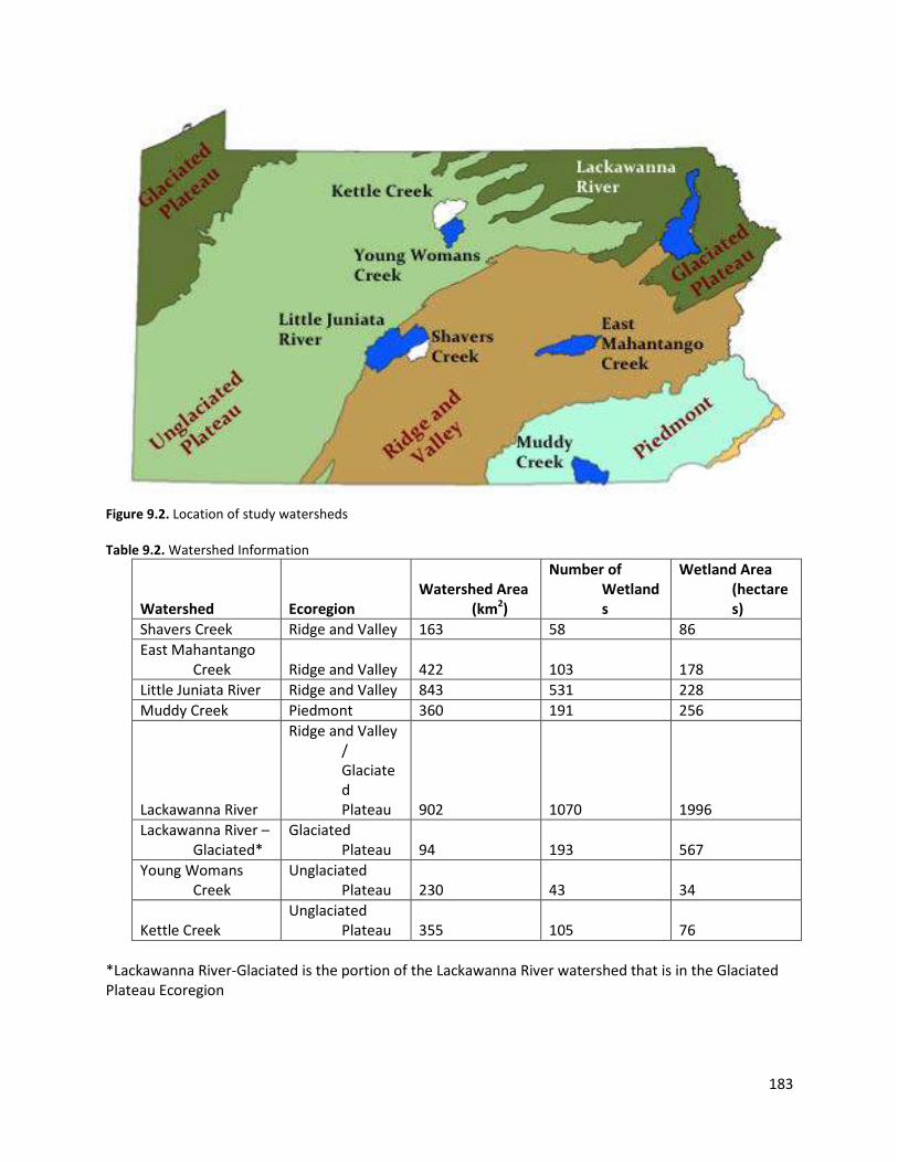
183

Figure 9.2. Location of study watersheds Table 9.2. Watershed Information

Watershed Ecoregion Watershed Area

(km2)

Number of Wetlands

Wetland Area (hectares)

Shavers Creek Ridge and Valley 163 58 86 East Mahantango

Creek Ridge and Valley 422 103 178 Little Juniata River Ridge and Valley 843 531 228 Muddy Creek Piedmont 360 191 256

Lackawanna River

Ridge and Valley / Glaciated Plateau 902 1070 1996

Lackawanna River – Glaciated*

Glaciated Plateau 94 193 567

Young Womans Creek

Unglaciated Plateau 230 43 34

Kettle Creek Unglaciated

Plateau 355 105 76 *Lackawanna River-Glaciated is the portion of the Lackawanna River watershed that is in the Glaciated Plateau Ecoregion

184

Land-use varied across each watershed (Figure 9.3), with watersheds in the Ridge and Valley dominated by forest (50-70%) and agriculture (20-40%), with few developed areas (5-10%). Muddy Creek watershed, within the Piedmont ecoregion, was dominated by agriculture (67%) and forested land-use (30%). The Lackawanna River watershed was primarily forested (66%), with some development (20%). While the portion of the Lackawanna River watershed that was within the Glaciated Plateau ecoregion was similarly forested (67%), it had proportionally more agriculture (22%) compared with the entire watershed (7%). The Unglaciated Plateau watersheds were primarily dominated by forested land-use (> 93%).

Figure 9.3. Land-use by watershed Projected Changes to Watersheds. Changes in groundwater levels between the historic and future climate scenarios were categorized as lower (drier) for drops greater than 3cm, higher (wetter) for increases greater than 3cm, and stable if changes in the future groundwater elevation were within 3cm of the historic level. The 3cm change value was selected because it represents 10% of the rooting depth of most wetland vegetation. On an annual basis, 11% of the approximately 2400 km2 in the 7 modeled Pennsylvania watersheds experienced drier conditions, 37% of the area was wetter, and the remaining 51% (1266 km2) remained stable. These values changed significantly when seasonal data was extracted from the annual results. For example, during the winter (December, January, February), 61% of the modeled land experienced wetter conditions, with only 32% remaining stable. Conversely, during the summer (June, July, August) 70% of the modeled land was drier, with only 19% remaining stable (Figure 9.4).

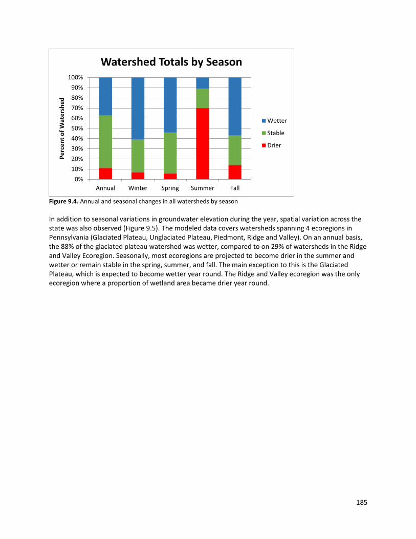
185

Figure 9.4. Annual and seasonal changes in all watersheds by season In addition to seasonal variations in groundwater elevation during the year, spatial variation across the state was also observed (Figure 9.5). The modeled data covers watersheds spanning 4 ecoregions in Pennsylvania (Glaciated Plateau, Unglaciated Plateau, Piedmont, Ridge and Valley). On an annual basis, the 88% of the glaciated plateau watershed was wetter, compared to on 29% of watersheds in the Ridge and Valley Ecoregion. Seasonally, most ecoregions are projected to become drier in the summer and wetter or remain stable in the spring, summer, and fall. The main exception to this is the Glaciated Plateau, which is expected to become wetter year round. The Ridge and Valley ecoregion was the only ecoregion where a proportion of wetland area became drier year round.

0%10%20%30%40%50%60%70%80%90%

100%

Annual Winter Spring Summer Fall

Perc

ent o

f Wat

ersh

ed

Watershed Totals by Season

Wetter

Stable

Drier

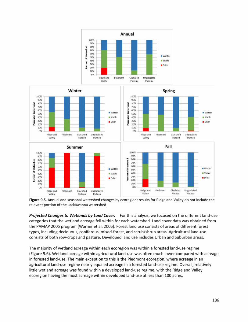
186

Figure 9.5. Annual and seasonal watershed changes by ecoregion; results for Ridge and Valley do not include the relevant portion of the Lackawanna watershed Projected Changes to Wetlands by Land Cover. For this analysis, we focused on the different land-use categories that the wetland acreage fell within for each watershed. Land cover data was obtained from the PAMAP 2005 program (Warner et al. 2005). Forest land use consists of areas of different forest types, including deciduous, coniferous, mixed-forest, and scrub/shrub areas. Agricultural land-use consists of both row-crops and pasture. Developed land use includes Urban and Suburban areas. The majority of wetland acreage within each ecoregion was within a forested land-use regime (Figure 9.6). Wetland acreage within agricultural land-use was often much lower compared with acreage in forested land-use. The main exception to this is the Piedmont ecoregion, where acreage in an agricultural land-use regime nearly equaled acreage in a forested land-use regime. Overall, relatively little wetland acreage was found within a developed land-use regime, with the Ridge and Valley ecoregion having the most acreage within developed land-use at less than 100 acres.

187

Figure 9.6. Total wetland acreage within each land-use regime by ecoregion; results for Ridge and Valley do not include the relevant portion of the Lackawanna watershed Of the wetland acreage within an agricultural land-use regime, the majority is projected to remain stable or become wetter (Figure 9.7). Only the Ridge and Valley ecoregion had any wetland acreage projected to become drier, though the majority of wetland acreage was still projected to remain stable within this ecoregion. In both the Glaciated Plateau and the Piedmont, more wetland acreage was projected to become wetter than to remain stable, while in the Unglaciated Plateau, all wetland acreage within agricultural land-use regimes was projected to remain stable. These results, in combination with the seasonal signal, can be used to outline some broad areas of management actions to consider. For example, the Ridge and Valley ecoregion was the only ecoregion that had any wetland acreage projected to become drier on an annual basis in both forested and agricultural land cover, and drier conditions were most pronounced in summer. Suggested management actions would therefore be those that emphasize infiltration and water retention during the wetter times of the year.

0

100

200

300

400

500

600

700

800

900

1000

Gla

ciat

ed P

late

au

Pied

mon

t

Ridg

e an

d Va

lley

Ung

laci

ated

Pla

teau

Gla

ciat

ed P

late

au

Pied

mon

t

Ridg

e an

d Va

lley

Ung

laci

ated

Pla

teau

Gla

ciat

ed P

late

au

Pied

mon

t

Ridg

e an

d Va

lley

Ung

laci

ated

Pla

teau

Agriculture Forest Developed

Acre

s

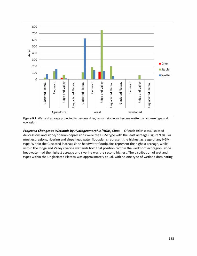
188

Figure 9.7. Wetland acreage projected to become drier, remain stable, or become wetter by land-use type and ecoregion Projected Changes to Wetlands by Hydrogeomorphic (HGM) Class. Of each HGM class, isolated depressions and slope/riparian depressions were the HGM type with the least acreage (Figure 9.8). For most ecoregions, riverine and slope headwater floodplains represent the highest acreage of any HGM type. Within the Glaciated Plateau slope headwater floodplains represent the highest acreage, while within the Ridge and Valley riverine wetlands hold that position. Within the Piedmont ecoregion, slope headwater had the highest acreage and riverine was the second highest. The distribution of wetland types within the Unglaciated Plateau was approximately equal, with no one type of wetland dominating.

0

100

200

300

400

500

600

700

800

Gla

ciat

ed P

late

au

Pied

mon

t

Ridg

e an

d Va

lley

Ung

laci

ated

Pla

teau

Gla

ciat

ed P

late

au

Pied

mon

t

Ridg

e an

d Va

lley

Ung

laci

ated

Pla

teau

Gla

ciat

ed P

late

au

Pied

mon

t

Ridg

e an

d Va

lley

Ung

laci

ated

Pla

teau

Agriculture Forest Developed

Acre

s

Drier

Stable

Wetter

189

Figure 9.8. Total wetland acreage within each HGM class by ecoregion Isolated depression acreage was projected to become wetter or remain stable in all ecoregions with the exception of the Ridge and Valley (Figure 9.9). Riverine wetland acreage was projected to become wetter in the Glaciated Plateau and the Piedmont ecoregions. The majority of Riverine acreage was projected to remain stable in the Ridge and Valley and the Unglaciated Plateau ecoregions, with a small amount of riverine acreage projected to become drier in the Ridge and Valley. The majority of Slope Headwater Floodplain acreage was projected to remain stable across the Piedmont, Ridge and Valley, and Unglaciated Plateau, while the majority of slope headwater floodplains in the Glaciated Plateau are projected to become wetter. Again, the Ridge and Valley was the only ecoregion where slope headwater floodplain acreage was projected to become drier. Slope/riparian depression acreage was projected to become wetter in the Glaciated Plateau, while the majority of slope/riparian depression acreage in the Piedmont, Ridge and Valley, and Unglaciated Plateau were projected to remain stable. The Ridge and Valley was the only ecoregion where slope/riparian depression acres were projected to become drier. Because of their direct connection to the bodies of water that people use for drinking water and recreation, riverine, slope headwater floodplains, and slope/riparian depression wetlands are often targeted for protection and restoration. While the majority of wetland acreage for these three wetland types is projected to remain stable across most ecoregions, some riverine and slope headwater wetlands in the Ridge and Valley may become drier. Thus any management efforts to protect wetlands from the effects of climate change should be focused on these wetlands so that they are able to continue providing water quality improvements to nearby water-bodies.

0

200

400

600

800

1000

1200

Gla

ciat

ed P

late

au

Pied

mon

t

Ridg

e an

d Va

lley

Ung

laci

ated

Pla

teau

Gla

ciat

ed P

late

au

Pied

mon

t

Ridg

e an

d Va

lley

Ung

laci

ated

Pla

teau

Gla

ciat

ed P

late

au

Pied

mon

t

Ridg

e an

d Va

lley

Ung

laci

ated

Pla

teau

Gla

ciat

ed P

late

au

Pied

mon

t

Ridg

e an

d Va

lley

Ung

laci

ated

Pla

teau

Isolated Depression Riverine Slope HeadwaterFloodplain

Slope/ RiparianDepression

Acre

s

190

Figure 9.9. Wetland acreage projected to become drier, remain stable, or become wetter by HGM type and ecoregion Projecting Changes to Specific Ecosystem Services. Because of the importance of water quality improvements provided by wetlands, there is great interest in being able to predict how climate change may affect the ability of wetlands to provide these services. However, while the evolution of hydrologic modeling tools has proceeded at a rapid rate, the necessary fine-grain resolution needed to answer these questions may not be presently available. For example, one water quality improvement provided by wetlands is the removal of excess nitrate from upland runoff via denitrification. Denitrification is an anaerobic process, and previous research has found that depth to water table has a large impact on denitrification rates (Hefting et al. 2004). Denitrification has been found to be minimal when the water table is lower than 40cm below ground level, and is most prominent when the water table is between 10cm and 30cm below ground level (Hefting et al. 2004). Because PIHM is able to predict water table elevations over geographic space under future climate scenarios, we tried to use the PIHM model to predict if wetland capacity for denitrification would increase, remain stable, or decrease under future climate conditions. Hydrologic criterion important to denitrification (10 to 30cm depth to water table) were selected, and we examined whether the acreage within the hydrologic criterion changed between the historic and future PIHM scenarios. It soon became apparent that the grain of the modeling elements were not small enough to properly assess this question (the elements, while of varying sizes, often span multiple acres). This makes detection of a loss or gain of wetland acreage difficult, especially if loss or gain occurs at the edges of wetlands less than an acre in size. In order to properly assess loss or gain of wetland acreage at the edge of wetlands, where it is likely to occur, modeling elements will need to be of a much finer grain, likely smaller than an acre. However, general specification of wetter/stable/drier conditions may be appropriate for general statements concerning changes in habitat conditions, such as plant community composition. Preliminary results of a study examining the impact of climate change on wetland plant community composition across the commonwealth suggests decreases

0

100

200

300

400

500

600

700

800

900

Gla

ciat

ed P

late

au

Pied

mon

t

Ridg

e an

d Va

lley

Ung

laci

ated

Pla

teau

Gla

ciat

ed P

late

au

Pied

mon

t

Ridg

e an

d Va

lley

Ung

laci

ated

Pla

teau

Gla

ciat

ed P

late

au

Pied

mon

t

Ridg

e an

d Va

lley

Ung

laci

ated

Pla

teau

Gla

ciat

ed P

late

au

Pied

mon

t

Ridg

e an

d Va

lley

Ung

laci

ated

Pla

teau

Isolated Depression Riverine Slope HeadwaterFloodplain

Slope/ RiparianDepression

Acre

s

Drier

Stable

Wetter

191

in Floristic Quality Assessment Index (FQAI) scores in slope wetlands of the Ridge and Valley ecoregion under a modeled future climate scenario. This decrease in FQAI scores is partially caused by an increase of both native and non-native invasive plant species in the study wetlands. While these early results only focus on a small portion of the resource within the commonwealth, ongoing research intends to further explore the impact of climate change on wetland plant community composition across additional ecoregions and HGM classes.

9.5 Conclusions and Recommendations The concept of vulnerability and its components (exposure, sensitivity, and adaptive capacity) allows a more informed examination of the potential impacts of climate change on aquatic resources, and the identification of potential management techniques to mitigate some of these. Because it is the driver of aquatic ecosystem processes, we chose to articulate vulnerability through changes in hydrologic regime, explicitly as wetter/stable/drier conditions. Vulnerabilities were able to be more explicitly evaluated in this update, due to the analysis of hydrologic conditions in seven watersheds selected to be representative of a range of ecoregions, wetland HGM classes, and predominant land cover types. The analysis reveals that exposure will vary across the Commonwealth by ecoregion and wetland type. Although annual conditions showed little change, seasonal changes in hydrologic regime are the primary story, with one watershed showing much wetter conditions annually and most watersheds exhibiting profoundly drier conditions in summer; our analysis showed striking results in the Ridge and Valley, Piedmont, and Unglaciated Plateau ecoregions. Sensitivity is based primarily on condition, which is generally determined by anthropogenic activity. While the majority of wetlands are found in forested land cover settings, the high percentage of agricultural and developed land covers in certain ecoregions and around certain wetland types reveals aquatic resources that are already compromised in their ability to provide ecosystem services. Thus, these systems will suffer even further decline if the local hydrologic conditions change as a result of climate. Recommendations for increasing adaptive capacity are the following:

• Protection of existing stream and wetland habitat, especially intact habitat for identified species of interest, such as eastern brook trout (EBTJV 2008).

• Maintenance of riparian forests for moderation of stream temperature and treatment of run-off from adjoining lands, especially in forested and agricultural land use settings

• Restoration of aquatic ecosystems such as streams and wetlands wherever possible • Minimize groundwater pumping for irrigation, human consumption, etc., that removes water

from high importance aquatic and wetland ecosystems. Maintenance of groundwater levels across all wetland systems are especially important, due to a projected drying of some systems during the growing season.

References Adger, W. N. 2006. Vulnerability. Global Environmental Change 16:268–281. Amoros, C., and G. Bornette. 2002. Connectivity and biocomplexity in waterbodies of riverine

floodplains. Freshwater Biology 47:761-776. Angeler, D. G., and M. Alvarez-Cobelas. 2005. Island biogeography and landscape structure: integrating

ecological concepts in a landscape perspective of anthropogenic impacts in temporary wetlands. Environmental Pollution 138:420–424.

192

Balcombe, C.K., J.T. Anderson, J.S. Rentch, W.N. Grafton, R.H. Fortney, W.S. Kordek. 2005a. A comparison of plant communities in mitigation and reference wetlands in the mid-Appalachians. Wetlands. 25: 130-142.

Balcombe, C.K., J.T. Anderson, R.H. Fortney, and W.S. Kordek 2005b. Vegetation, invertebrate, and wildlife community rankings and habitat analysis of mitigation wetlands in West Virginia. Wetlands Ecology and Management. 13: 517-530.

Bayley, P.B. 1995. Understanding large river-floodplain ecosystems. Bioscience 45: 53-75. Beecher, S., & Thaler, T., Griffith, G., Perry, A.., Crossett, T., Rasker, R. (Eds). 2013. Adapting to a

Changing Climate: Risks & Opportunities for the Upper Delaware River Region. Model Forest Policy Program in association with Common Waters Partnership, Pinchot Institute for Conservation the Cumberland River Compact and Headwaters Economics; Sagle, ID

Brinson, M.M. 1993. A Hydrogeomorphic Classification for Wetlands. Vicksburg, MS, USA. Brooks, R. P., D. H. Wardrop, and J. A. Bishop. 2004. Assessing wetland condition on a watershed basis in

the mid-Atlantic region using synoptic land-cover maps. Environmental monitoring and assessment 94:9–22.

Bunn, S. E., and A. H. Arthington. 2002. Basic principles and ecological consequences of altered flow regimes for aquatic biodiversity. Environmental Management 30(4):492-507.

Burkett, V.R., and J. Kusler. 2000. Climate change: potential impacts and interactions in wetlands of the United States. JAWA 36(2): 313-320.

Castelle, A. J., A. W. Johnson, and C. Conolly. 1994. Wetland and stream buffer size requirements—a review. Journal of Environment Quality 23:878–882.

Cedfeldt, P. T., M. Watzin, and B. Richardson. 2000. Using GIS to identify functionally significant wetlands in the northeastern United States. Environmental Management 26:13–24.

Crosbie, B., and P. Chow-fraser. 1999. Percentage land use in the watershed determines the water and sediment quality of 22 marshes in the Great Lakes basin. Canadian journal of fisheries and aquatic sciences 56:1781–1791.

Cuffney, T. F. 1988. Input , movement and exchange of organic matter within a subtropical coastal blackwater river-floodplahi system. Freshwater Biology 19:305–320.

Dillon, P. J., and L. Molot. 1997. Effect of landscape form on export of dissolved organic carbon, iron, and phosphorus from forested stream catchments. Water Resources Research 33:2591–2600.

Dosskey, M. G., and P. M. Bertsch. 1994. Forest sources and pathways of organic matter transport to a blackwater stream: a hydrologic approach. Biogeochemistry 24:1–19.

Dukes, J. S., and H. A. Mooney. 1999. Does global change increase the success of biological invaders? Trends in Ecology and Evolution 14:135-139.

EBTJV (Eastern Brook Trout Joint Venture), Conservation Strategy/Habitat Workgroup. 2008. Conserving the Eastern Brook Trout: Action Strategies. Available: www.easternbrooktrout.org. (May 2009).

EBTJV (Eastern Brook Trout Joint Venture). 2006. Eastern brook trout: status and threats. Prepared by Trout Unlimited, Arlington, Virginia, for the Eastern Brook Trout Joint Venture. 36 p. Available: www.easternbrooktrout.org. (May 2009).

Fennessy, M. S., A. D. Jacobs, and M. E. Kentula. 2007. An evaluation of rapid methods for assessing the ecological condition of wetlands. Wetlands 27:543–560.

Firth, P., and S. G. Fisher. 1991. Global climate change and freshwater ecosystems. Springer-Verlag, New York, New York, USA.

Fisher, A. 2000. Preliminary findings from the Mid-Atlantic regional assessment. Climate Research 14:261-269.

Fore, L. S., J. W. Karr, and L. Conquest. 1994. Statistical properties of an index of biological integrity used to evaluate water resources. Canadian Journal of Fisheries and Aquatic Sciences 51:1077–1087.

Gilliam, J. W. 1994. Riparian Wetlands and Water Quality. Journal of Environment Quality 23:896–900.

193

Gitay, H., Brown, S., Easterling, W., Jallow, B., 2001. Ecosystems and their goods and services. In: McCarthy, J., Canziani, O., Leary, N., Dokken, D., White, K. (Eds.), Climate Change 2001: Impacts, Adaptation, and Vulnerability. Cambridge University Press, NewYork, pp. 235–342.

Godwin, C.M., Arthur, M.A., and Carrick, H.J. 2009. Periphyton nutrient status in a temperate stream with mixed land-uses: implications for watershed nitrogen storage. Hydrobiologia 623(1): 141-152.

Godwin, C.M., and Carrick, H.J. 2007. Spatio-temporal variation of periphyton biomass and production in a temperate spring-fed stream. Aquatic Ecology 42: 583–595.

Griscom, B., M. McKenney-Easterling, W.L. Myers, A. McQueen, J.A. Bishop, G. Rocco, J. French, K.C. Hychka, A. Bayard, T. O’Connell, G.P. Patil, C. Taillie, G. D. Constantz and R.P. Brooks. 2007. Classifying and prioritizing watersheds for protection and restoration. Final report to U.S. Environmental Protection Agency, Agreement No. R830593.

Harper, M. P., and B. L. Peckarsky. 2006. Emergence cues of a mayfly in a high-altitude stream ecosystem: potential response to climate change. Ecological Applications 16(2):612-621.

Haycock, N. E., and G. Pinay. 1993. Groundwater nitrate dynamics in grass and poplar vegetated riparian buffer strips during the winter. Journal of environmental quality 22:273–278.

Hefting, M., J. C. Clément, D. Dowrick, a. C. Cosandey, S. Bernal, C. Cimpian, a. Tatur, T. P. Burt, and G. Pinay. 2004. Water table elevation controls on soil nitrogen cycling in riparian wetlands along a European climatic gradient. Biogeochemistry 67:113–134.

Houlahan, J. E., and C. S. Findlay. 2004. Estimating the “critical” distance at which adjacent land-use degrades wetland water and sediment quality. Landscape Ecology 19:677–690.

Hudy, M., T. M. Thieling, N. Gillespie, and E. P. Smith. 2008. Distribution, status, and land use characteristics of subwatersheds within the native range of brook trout in the eastern United States. North American Journal of Fisheries Management 28: 1069-1085.

Hudy, M., T. M. Thieling, N. Gillespie, and E. P. Smith. 2005. Distribution, status, and threats to brook trout within the eastern United States. Final report to the steering committee of the Eastern Brook Trout Joint Venture. 77 pp. Available: www.easternbrooktrout.org. (May 2009).

Humphries, P., A.J. King, and J.D. Koehn. 1999. Fish, flows and flood plains: links between freshwater fishes and their environment in the Murray-Darling River system, Australia. Environmental Biology of Fishes 56: 129-151.

Jordan, T. E., D. F. Whigham, K. H. Hofmockel, and M. a Pittek. 2003. Nutrient and sediment removal by a restored wetland receiving agricultural runoff. Journal of environmental quality 32:1534–47.

Karr, J. R., and E. W. Chu. 1999. Restoring life in running waters: better biological monitoring. Island Press, Washington, D. C.

Keller, W. T. 1979. Management Humphries, P., and D. S. Baldwin. 2003. Drought and aquatic ecosystems: an introduction. Freshwater Biology 48:1141-1146.

Kenny, J.F., Barber, N.L., Hutson, S.S., Linsey, K.S., Lovelace, J.K., and Maupin, M.A., 2009, Estimated use of water in the United States in 2005: U.S. Geological Survey Circular 1344, 52 p

Kreeger, D., J. Adkins, P. Cole, R. Najjar, D. Velinsky, P. Conolly, and J. Kraeuter. June 2010. Climate Change and the Delaware Estuary: Three Case Studies in Vulnerability Assessment and Adaptation Planning. Partnership for the Delaware Estuary, PDE Report No. 10-01. 1 –117 pp.

Leibowitz, S. G., and K. C. Vining. 2003. Temporal connectivity in a prairie pothole complex. Wetlands 23:13–25.

Lenat, D. R., and J. K. Crawford. 1994. Effects of land use on water quality and aquatic biota of three North Carolina Piedmont streams. Hydrobiologia 294:185–199.

Leopold, L.B., M.G. Wolman, and J.P. Miller. 1964. Fluvial processes in geomorphology. San Francisco, California: W.H. Freeman.

194

Lowrance R, L.S. Altier, J.D. Newbold, R.R. Schnabel, P.M. Groffman, J.M. Denver, D.L. Correll, J.W. Gilliam, and J.L. Robinson. 1997. Water quality functions of riparian forest buffers in Chesapeake Bay watersheds. Environmental Management. 21:687–712

McIlnay, D. P. 2002. Juniata, River of Sorrows. Seven Oaks Press, Hollidaysburg, PA, USA. McKnight, D. 2001. Freshwater ecosystems and climate change: recent assessments and

recommendations. Limnology and Oceanography Bulletin 10:61-65. Millennium Ecosystem Assessment, 2005. ECOSYSTEMS AND HUMAN WELL-BEING: WETLANDS AND

WATER Synthesis. World Resources Institute, Washington, DC. http://www.millenniumassessment.org/documents/document.358.aspx.pdf

Miller, S. J., D. H. Wardrop, W. M. Mahaney, and R. P. Brooks. 2006. A plant-based index of biological integrity (IBI) for headwater wetlands in central Pennsylvania. Ecological Indicators 6:290–312.

Mitsch, W.J. and J.G. Gosselink. 1993. Wetlands. New York: Wiley & Sons. Moore, M. V., M. L. Pace, J. R. Mather, P. S. Murdoch, R. W. Howarth, C. L. Folt, C. Y. Chen, H. F.

Hemond, P. A. Flebbe, and C. T. Driscoll. 1997. Potential effects of climate change in freshwater ecosystems of the New England/Mid-Atlantic Region. Hydrological Processes 11:925-947.

Moorhead, K.K. 2001. Seasonal water table dynamics of a southern Appalachian floodplain and associated fen. Journal of the American Water Resources Association. 37: 105-114.

Mountain, D. G. 2002. Potential consequences of climate change for the fish resources in the Mid-Atlantic Region. American Fisheries Society 32:185-194.

Mulholland, P. J. 1981. Organic carbon flow in a swamp-stream ecosystem. Ecological Monographs 51:307–322.

Myers, W.L., M. McKenney-Easterling, K.C. Hychka, B. Griscom, J.A. Bishop, A. Bayard, G.L. Rocco, R.P. Brooks, G. Constantz, G. P. Patil and C. Taillie. 2006. Contextual clustering for configuring collaborative conservation of watersheds in the Mid-Atlantic Highlands. Environmental and Ecological Statistics, http://www.springerlink.com/content/1573-3009/ 13(4):391-407.

Omernick, J. 1976. The influence of land use on stream nutrient levels. United States Environmental Protection Agency. EPA-60013-76-014US

Palmer, S. M., D. Hope, M. F. Billett, J. J. C. Dawson, and C. L. Bryant. 2001. Sources of organic and inorganic carbon in a headwater stream : Evidence from carbon isotope studies. Biogeochemistry 52:321–338.

Parmesan, C., and G. Yohe. 2003. A globally coherent fingerprint of climate change impacts across natural systems. Nature 421 (2 January 2003): 37-42.

Peckarsky, B. L., B. W. Taylor, A. R. McIntosh, M. A. McPeek, and D. A. Lytle. 2001. Variation in mayfly size at metamorphosis as a developmental response to risk of predation. Ecology 82:740-757.

Poff, N.L., and J.D. Allan. Functional organization of stream fish assemblages in relation to hydrological variability. Ecology 76(2): 606-627.

Poff, N.L., M.M. Brinson, and J.W. Day. 2002. Aquatic Ecosystems and Global Climate Change: Potential Impacts on Inland Freshwater and Coastal Wetland Ecosystems in the United States. Prepared for the Pew Center on Global Climate Change, January 2002. 56 pp.

Poff, N. L., S. Tokar, and P. Johnson. 1996. Stream hydrological and ecological responses to climate change assessed with an artificial neural network. Limnology and Oceanography 41(5):857-863.

Poff, N. L. and J. V. Ward. 1989. Implications of streamflow variability and predictability for lotic community structure: a regional analysis of streamflow patterns. Canadian Journal of Fisheries and Aquatic Science 46:1805-1818.

Polsky, C., R. Neff, and B. Yarnal. 2007. Building comparable global change vulnerability assessments: The vulnerability scoping diagram. Global Environmental Change 17:472–485.

Postel, S.L., and S.R. Carpenter. 1997. “Freshwater Ecosystem Services.” In Nature’s Services: Societal Dependence on Natural Ecosystems. G.D. Daily, ed. Island Press, Washington, DC, pp. 195-214.

195

Qu, Y. and C.J. Duffy. 2007. A semidiscrete finite volume formulation for multiprocess watershed simulation. Water Res. Research. 43, W08419, doi:10.1029/2006WR005752

Rogers, C. E., and J. P. McCarty. 2000. Climate change and ecosystems of the Mid-Atlantic Region. Climate Research 14(3):235-244.

Rosenzweig, C., G. Casassa, D.J. Karoly, A. Imeson, C. Liu, A. Menzel, S. Rawlins, T.L. Root, B. Seguin, P. Tryjanowski, 2007: Assessment of observed changes and responses in natural and managed systems. Climate Change 2007: Impacts, Adaptation and Vulnerability. Contribution of Working Group II to the Fourth Assessment Report of the Intergovernmental Panel on Climate Change, M.L. Parry, O.F. Canziani, J.P. Palutikof, P.J. van der Linden and C.E. Hanson, Eds., Cambridge University Press, Cambridge, UK, 79-131.

Rossell, I.M. and Kesgen, J.M. 2003. The distribution and fruiting of red and black chokecherry (Aronia arbutifolia and A. melanocarpa) in a southern Appalachian fen. Journal of the Torrey Botanical Society. 130: 202-205.

Roth, N. E., M. T. Southerland, G. M. Rogers, and J. H. Volstad. 2004. Maryland Biological Stream Survey 200-2004: Volume III. Ecological assessment of watersheds sampled in 2002. Maryland Department of Natural Resources, Annapolis, MD, U.S.A.

Roy, A. H., A. D. Rosemond, D. S. Leigh, M. J. Paul, and J. B. Wallace. 2003. Habitat-specific responses of stream insects to land cover disturbance: biological consequences and monitoring implications. Journal of the North American Benthological Society 22(2):292-307.

Schiff, S., R. Aravena, S. Trumbore, and P. Dillon. 1990. Dissolved organic carbon cycling in forested watersheds: a carbon isotope approach. Water Resources Research 26:2949–2957.

Sedell, J. R., G. H. Reeves, F. R. Hauer, J. A. Stanford, and C. P. Hawkins. 1990. Role of refugia in recovery from disturbances: modern fragmented and disconnected river systems. Environmental Management 14(5):711-724.

Sheldon, F., A.J. Boulton, and J.T. Puckridge. 2002. Conservation value of variable connectivity: aquatic invertebrate assemblages of channel and floodplain habitats of a central Australian arid-zone river, Cooper Creek. Biol. Cons. 103:13-31.

Snyder, C.D., J.A. Young, and B.M. Stout, III. 2006. Aquatic habitats of Canaan Valley, West Virginia: diversity and environmental threats. Northeastern Naturalist. 13: 333-352.

Smock, L. A. 1990. Spatial and temporal variation in organic matter storage in low-gradient, headwater streams. Archives of Hydrobiolgy 118:169-184.

Sweeney, B. W., J. K. Jackson, J. D. Newbold, and D. H. Funk. 1991. Climate change and the life histories and biogeography of aquatic insects in eastern North America. Pages 143-176 in P. Firth and S. G. Fisher, editors. Global climate change and freshwater ecosystems. Springer-Verlag, New York, New York, USA.

Suen, J. P. 2008. Potential impacts to freshwater ecosystems caused by flow regime alteration under changing climate conditions in Taiwan. Hydrology and Earth Systems Sciences Discussions 5:3005-30032.

Taylor, J. R., M. A. Cardamone, and W. J. Mitsch. 1990. Pages 13-86 in J. G. Gosselink, L. C.Lee, and T. A. Muir, editors. Ecological Processes and Cumulative Impacts: Illustrated by Bottomland Hardwood Wetland Ecosystems. Lewis Publishers, MI.

Tiner, R.W. 1990. Pennsylvania's Wetlands: Current Status and Recent Trends. Pennsylvania Bureau of Water Resources Management. Harrisburg, Pennsylvania.USA.

Tockner, K., F. Malard, and J. V. Ward. 2000. An extension of the flood pulse concept. Hydrological Processes 14:2861-2883.

Trebitz, A. S., J. C. Brazner, A. M. Cotter, M. L. Knuth, J. a. Morrice, G. S. Peterson, M. E. Sierszen, J. A. Thompson, and J. R. Kelly. 2007. Water Quality in Great Lakes Coastal Wetlands: Basin-wide

196

Patterns and Responses to an Anthropogenic Disturbance Gradient. Journal of Great Lakes Research 33:67–85.

US EPA. 2006. Draft Wadeable Streams Assessment: A Collaborative Survey of the Nation’s Streams. U.S. Environmental Protection Agency, Office of Water, Washington, DC, U.S.A. EPA 841-B-06-002.

U.S. EPA. 2009. Geographic information systems analysis of the surface drinking water provided by intermittent, ephemeral, and headwater streams in the U.S. http://water.epa.gov/lawsregs/guidance/wetlands/surface_drinking_water_index.cfm, last accessed 12/18/2014.

Vörösmarty, C.J., P. Green, J. Salisbury, and R.B. Lammers. 2000. “Global Water Resources: Vulnerability from Climate Change and Population Growth.” Science 289:284-288.

Ward, J. V. 1992. Aquatic insect ecology. 1. Biology and habitat. John Wiley and Sons, New York, New York, USA.

Wardrop, D. H., M. E. Kentula, S. F. Jensen, D. L. Stevens, K. C. Hychka, and R. P. Brooks. 2007. Assessment of wetlands in the Upper Juniata watershed in Pennsylvania, USA using the hydrogeomorphic approach. Wetlands 27:432–445.

Warner, E., Myers, W., Bishop, J., Miller, D 2005 Land cover classification for Pennsylvania. Digital map data. Penn State Institutes of Energy and the Environment, Pennsylvania State University, University Park, Pennsylvania. In cooperation with the Pennsylvania Department of Conservation of Natural Resources, Harrisburg, Pennsylvania.

Watanabe, N. C., I. Mori, and I. Yoshitaka. 1999. Effect of water temperature on the mass emergence of the mayfly, Ephoron shigae, in a Japanese river (Ephemeroptera: Polymitarcyidae). Freshwater Biology 41:537-541.

Whigham, D. F., C. Chitterling, and B. Palmer. 1988. Impacts of freshwater wetlands on water quality: a landscape perspective. Environmental Management 12:663–671.

Winter, T.C. 2000. The vulnerability of wetlands to climate change: A hydrologic landscape perspective. JAWA 36(2): 305-311.

Woods, A., J. Omernick, and D. Brown. 1999. Level III and IV ecoregions of Delaware, Maryland, Pennsylvania, Virginia, and West Virginia. Page 57.

Zedler, Joy B. 2003. Wetlands at Your Service: Reducing Impacts of Agriculture at the Watershed Scale. Frontiers in Ecology and the Environment. 1(2): 65-72.

197

10 Coastal resources 10.1 Potential impact of climate change on southeastern Pennsylvania’s coastal resources Pennsylvania’s coastline on the Delaware Estuary extends from Morrisville, PA (across the river from Trenton, NJ) to Marcus Hook, PA (just north of the Delaware State border), a distance of 56 miles. This portion of the estuary is mostly fresh water and is home to diverse flora and fauna. Economic activity along this portion of the Delaware Estuary has long been very high and has resulted in severe water quality problems. Inputs of untreated or poorly treated sewage from large cities, such as Philadelphia and Camden, caused dramatic declines in oxygen concentration throughout the much of the 20th century, with severe impacts on economically and ecologically important anadromous fishes, such as sturgeon, shad, and striped bass (Breese et al., 2012). Other fauna, such as freshwater bivalve shellfish, which serve important ecological roles, including water filtration and habitat construction, were likely influenced by the dramatic changes in water quality. As a result of the Federal Clean Water Act, improvements in wastewater treatment were implemented, which led to substantial improvements in water quality and living resources. Climate change poses a threat to the fauna of the tidal freshwater portion of the Delaware estuary for two main reasons. First, warming will decrease the solubility of oxygen in water and will increase respiration rates, both of which will result in declines in dissolved oxygen concentration. Najjar (2015) estimates that, under the A2 emissions scenario, water temperature during the summer (when growth rates are highest) in the tidal freshwater region will increase 2.7 to 3.5 °C (4.9-6.3°F) (95% confidence range) by mid-century (2041-2070) with respect to the late 20th century. Building on the dissolved oxygen modeling of Tomaso and Najjar (2015), it is estimated that this warming will result in a dissolved oxygen concentration decline of about 20 mmol m-3 or 13% at the Ben Franklin Bridge (BFB, Philadelphia). Kahn et al. (2014) argue that a safe level of the 24-hour average oxygen concentration in the Delaware Estuary is 190 mmol m-3, which is above the current average summer level near the BFB (150 mmol m-3). Thus climate change will worsen the currently substandard water quality in the tidal freshwater region of the Delaware Estuary. The second reason that climate change threatens tidal freshwater fauna is through salt intrusion associated with sea-level rise and summertime streamflow declines. Najjar (2015) estimate that, by mid-century in the upper Delaware Estuary, sea level will increase by 0.40 m and summer streamflow will decrease by 19%. Using the statistical salinity models of Ross et al. (2015), the streamflow decline corresponds to a salinity increase at the Ben Franklin Bridge (Philadelphia) of less than 0.01 part per thousand (ppt), which is small compared to the current annual-mean salinity of 0.12 ppt. Sea-level rise is also expected to cause a small increase in salinity in the tidal freshwater region, moving the mean position of the 0.5-ppt isohaline landward by 4 km. Hence, the existing research suggests modest impact of climate change on salinity of the upper Delaware Estuary. The freshwater tidal wetlands along Pennsylvania’s southeastern coast are a rare, diverse, and ecologically important resource. Miller et al. (2012) estimate that there are 1195 acres of tidal wetlands in southeastern Pennsylvania, 55% unvegetated, 26% with emergent vegetation, and 19% with scrub/shrub and forested wetland. The present tidal wetland area in Pennsylvania is probably a few percent of its pre-European levels (Kreeger and Padeletti, 2011). Furthermore, Miller et al. (2012) document declines in tidal wetland area in southeastern Pennsylvania that continue to the present. Climate change poses a threat to these wetlands because of salinity intrusion and sea-level rise. As

198

noted above, salt intrusion impacts may be modest. Sea-level rise, however, has the potential to drown wetlands if their accretion rates are less than rates of sea-level rise. The potential for horizontal migration is low in southeastern Pennsylvania due to extensive development. In summary, climate change has the potential to exacerbate the currently highly stressed state of Pennsylvania’s tidal wetlands.

References Breese, G., Bright, G., Burke, D., Clark, J., Kahn, D., Kreeger, D., Kraeuter, J., Mohler, J., Wong, R., 2012.

Chapter 6 -- Living Resources. Technical Report for the Delaware Estuary and Basin, PDE Report No. 12-01. Partnership for the Delaware Estuary, pp. 166-224.

Kahn, D., Kreeger, D.A., Mohler, J., Silldorff, E., Kilham, S., Eldridge, W., 2014. Dissolved oxygen standards to protect aquatic life in the tidal freshwater Delaware River, A brief of the Science and Technical Advisory Committee, Partnership for the Delaware Estuary, 21 pp.

Kreeger, D., Padeletti, A., 2011. The condition of tidal freshwater wetlands in Pennsylvania, PDE Report No. 11-07. Partnership for the Delaware Estuary, 33 pp.

Miller, D., Padeletti, A., Kreeger, D., Homsey, A., Tudor, R., Creveling, E., DePhilip, M.M., Pindar, C., 2012. Chapter 5 -- Aquatic Habitats. Technical Report for the Delaware Estuary and Basin, PDE Report No. 12-01. Partnership for the Delaware Estuary, pp. 119-165.

Najjar, R.G., 2015. Potential impact of climate change on bivalves in the tidal freshwater region of the Delaware River: Final report to Pennsylvania Sea Grant. The Pennsylvania State University, University Park, Pennsylvania.

Ross, A.C., Najjar, R.G., Li, M., Mann, M.E., Ford, S.E., Katz, B., 2015. Sea-level rise and other influences on decadal-scale variations of salinity in a coastal plain estuary. Estuarine Coastal and Shelf Science 157, 79-92.

Tomaso, D., Najjar, R., 2015. Seasonal and interannual variations in the dissolved oxygen budget of an urbanized tidal river: The Upper Delaware Estuary. Journal of Geophysical Research: Biogeosciences, in revision.

2700-BK-DEP4494 8/2015