impacts of comprehensive climate and energy policy...
TRANSCRIPT
Impacts of Comprehensive Climate and Energy Policy Options
on the U.S. Economy » July 2010


Impacts of Comprehensive Climate and Energy Policy Options on the U.S. Economy !1
Foreword 3
Acronyms and Abbreviations 5
Executive Summary 6
Sections
Section 1 Introduction 16
Section 2 National Scale-up of State Actions: GHG Reduction Potential and Microeconomic Analysis of Climate Mitigation Options 18
Section 3Macroeconomic E!ects of Mitigation Options: REMI Model Analysis 28
Section 4Mitigation Option Implementation Jurisdiction and Programmatic Issues 55
Section 5Conclusions 62
Section 6References and Data Sources 70
AnnexesThe following Annexes to this report are available at energypolicyreport.jhu.edu:
Annex A Estimation Methodology for GHG Reduction Potential and Cost-E!ectiveness of Super Options
Annex BSuper Mitigation Options Descriptions
Annex C Description of the REM PI+ Model
Annex D Scale-up Approach for National REMI Inputs Preparation
Annex E Detailed REMI Model Simulation Results
Annex F Methodology for Analyzing Cap-and-Trade and Other Policies and Measures Using the REMI Model
» Table of Contents

Impacts of Comprehensive Climate and Energy Policy Options on the U.S. Economy !3
In environmental policymaking, states frequently act in advance of federal action and provide critical guidance and experience for national solutions. This is the case with climate change mitigation policy, which has evolved quickly in over 30 states in the last 5 years. Ironically, this wave of policy development has occurred during a time of economic uncertainty and high unemployment, when many question whether adopting mitigation measures to reduce greenhouse gas (GHG) emissions, including conserving or diversifying energy sources, might put overly burdensome and costly demands on the nation’s economic sectors or force energy cost increases that would further slow the economy and negatively impact jobs. Despite these concerns, many governors acted to address climate change in recognition of the urgency of the problem, the responsibility of the nation as a leading emi"er, and the opportunity for important benefits. At the same time, they have shown a"ention to the economic impacts and cost e!ectiveness of climate policies and measures.
To address economic security concerns related to national climate and energy policy, The Center for Climate Strategies (CCS) examined the likely impacts of nationwide climate policy implementation based upon climate actions plans developed in 16 states. Since 2004, CCS has worked with in 24 states with over 1,500 state-level stakeholders to formulate comprehensive, sector-based strategies to reduce GHG emissions and achieve energy and environmental co-benefits. The economic analysis of these plans reported in this paper indicates that these stakeholder-recommended policies can, if designed properly, actually spur the economy, create jobs and reduce energy prices while significantly reducing emissions.
Specifically, the policies developed address several sectors of the economy, including heat and power energy supply, manufacturing and industry, agriculture and forestry, transportation and land use, buildings and facilities, and waste management. A key finding is that carefully selected and designed sector-based GHG reduction policies can be highly cost e!ective, expand the economy, save consumers energy and money, improve public health, and reduce reliance on imported oil. For example, this analysis finds that 2.5 million net new jobs and a $159.6 billion expansion in U.S. GDP could result by 2020 if 23 major sector-based policies and measures in state climate action plans are implemented nationwide, while reducing projected energy prices. Furthermore, the nature of jurisdictional di!erences among local, state and federal governments indicates that to achieve these results all levels of government should have a role in implementing these measures. It is critically important that the design of new federal climate and energy policy take into account the innovative and e!ective measures many states and municipalities have already adopted or planned. This report should be highly useful to federal lawmakers and the administration as they continue to work to formulate a comprehensive national policy for climate and energy.
The study was primarily completed at the Center of Climate Strategies, a non-partisan, non-profit NGO, based in Washington, D.C., which is the leading organization in the nation providing support for state and regional climate action planning. CCS has provided technical assistance to more than forty states. Its signature stakeholder-based consensus-building process was used in the 16 states whose climate plan policies are the basis of this study. Additional states are using this stakeholder-based process and CCS is now working in other countries as well, to formulate and integrate state and federal climate and energy policy. CCS combines expertise in facilitation, technical analysis, and policy design to provide cu"ing-edge, collaborative decision-making. The CCS stakeholder approach builds high levels of consensus for the implementation of specific policy actions that address multiple public policy objectives including economic and energy security.
» Foreword

4! Johns Hopkins University and Center for Climate Strategies
The Johns Hopkins Washington, D.C. Center o!ers a range of advanced academic programs leading to the M.A. and M.B.A. degrees. Governmental Studies at the Hopkins Washington Center includes two master’s degree programs, the M.A. in Government and the M.A. in Global Security, and partnership programs for professional development and policy studies. In its partnerships for policy studies, the Center periodically publishes timely reports of pathbreaking work that can be"er inform an ongoing policy debate. This report to produce the work of CCS is such an e!ort and is intended to positively contribute to the current national debate over the economic implications of climate and energy policy options.
The primary authors of the study are: Thomas Peterson, President and CEO of CCS and Teaching Fellow, Johns Hopkins University and Je!rey Wennberg, Senior Project Manager at CCS, who coordinated the project, and organized and wrote major sections. Adam Rose, Research Professor at the University of Southern California’s School of Policy, Planning and Development (SPPD) and Dan Wei, Postdoctoral Research Associate, SPPD, USC, performed the macroeconomic analysis, deriving the employment, income and gross domestic product estimates for the scenarios that are the heart of this study. They were assisted by Noah Dormady, PhD student in SPPD. In addition, CCS’s team of experts updated sector analyses from the 16 states to develop of the microeconomic inputs to the study: Bill Dougherty of the Climate Change Research Group; David von Hippel of the Nautilus Institute; Hal Nelson of Claremont-McKenna College; Lewison Lem, Mike Lawrence, Jonathan Skolnik, Rami Chami and Sco" Williamson of Jack Fauce" Associates; and Steve Roe, Jim Wilson, Maureen Mullen, Brad Strode, Jackson Schreiber, Juan Maldonado, Jonathan Dorn, and Rachel Anderson of E.H. Pechan & Associates. This analysis was achieved using Regional Economic Models, Inc. (REMI) Policy Insight Plus (PI+) Modeling. Valuable consultation about the use of the model was provided by REMI sta! member Rod Motamedi.
The authors also acknowledge the contributions of external reviewers who provided comments on various dra#s of this report: Charles Colgan, Michael Lahr, Skip Laitner, Douglas Meade, and Dan Rickman. We also benefi"ed from comments on earlier dra#s by Carolyn Fischer. Additionally, June Taylor and Joan O’Callaghan of CCS and Kathy Wagner of Johns Hopkins University (JHU) provided editorial support. Stacey Maloney of JHU designed this publication. The contents and opinions expressed in this report are those of the authors, who are solely responsible for any errors and omissions. Funding was provided by the Town Creek Foundation, the Sea Change Foundation, the Emily Hall Tremaine Foundation, the Rockefeller Brothers Fund, the Merck Family Fund, the Mertz Gilmore Foundation, and the Turner Foundation.
Kathy Wagner, Ph.D.Director, Governmental Studies Johns Hopkins University , School of Arts and Sciences
Thomas Peterson, M.E.M. and M.B.A.President and CEO, Center for Climate Strategies Teaching Fellow Johns Hopkins University

Impacts of Comprehensive Climate and Energy Policy Options on the U.S. Economy !5
ACEEE American Council for an Energy-E$cient Economy
AEO Annual Energy Outlook
AFW Agriculture, Forestry and Waste Management [sector]
AASHTO American Association of State Highway and Transportation O$cials
APA American Power Act [Senate climate bill]
BRT bus rapid transit
CCS Center for Climate Strategies
CCSR carbon capture and storage or reuse
CGE computable generated equilibrium [model]
CHP combined heat and power
CO2 carbon dioxide
CO2e carbon dioxide equivalent
C&T cap-and-trade
DSM demand side management
E85 ethanol 85 [gasoline blend with up to 85% ethanol]
EEC energy e$ciency and conservation
EIA Energy Information Agency
EIS Energy-Intensive [Industrial] sector
ES Energy/Electricity Supply [sector]
ESD energy supply and demand
GAAMP Generally Accepted Agricultural Management Practices
GDP gross domestic product
GREET Greenhouse Gases, Regulated Emissions, and Energy Use in Transportation [model]
HDV heavy duty vehicles
HHS [U.S. Department of] Health and Human Services
HVAC heating, ventilating and air conditioning
IGCC integrated gasification combined cycle
Ind Industrial [sector]
I-O input-output [model]
K-L Kerry-Lieberman [Senate climate bill]
kgCO2!/gge kilograms of carbon dioxide per gasoline gallon equivalent
LDV light duty vehicles
LFG land fill gas
ME macroeconometric [model]
MMtCO2e million metric tons of carbon dioxide equivalent
MP mathematical programming [model]
MPG miles per gallon
MSW municipal solid waste
NG natural gas
NPS new-source performance standards
NPV net present value
N2O nitrous oxide
O&M operation and maintenance
ORNL Oak Ridge National Laboratory
PI+ Policy Insight Plus
RCI Residential, Commercial and Industrial [sector]
RECs Renewable Energy Certificates
REMI Regional Economic Models, Inc.
REMI PI+ Regional Economic Models, Inc. Policy Insight Plus [model]
RPS Renewable Portfolio Standard
SGA Southern Governors’ Association
TLU Transportation and Land Use [sector]
TRB Transportation Research Board
TRUs trailer refrigeration units
TSE truck stop electrification
USDOE United States Department of Energy
USEPA United States Environmental Protection Agency
VMT vehicle miles traveled
VISION Voluntary Innovative Sector Initiatives [of USDOE]
» Acronyms and Abbreviations

6! Johns Hopkins University and Center for Climate Strategies
The national debate over federal climate policy and its impact on the broader economy should be informed by the experience of the states and their stakeholders, which have been engaged in broad scale comprehensive climate policy planning, analysis and implementation since 2005. This study compiles and updates the findings of 16 comprehensive state climate action plans and extrapolates the results to the nation. The study then takes those results and using a widely accepted econometric model projects the national impact of these policies on employment, incomes, gross domestic product (GDP) and consumer energy prices. Finally, using the bo"om-up data developed by the states and aggregated here, the study models the national impact of major features of the Kerry-Lieberman (K-L) bill currently under consideration in Congress.
These state action plans and supporting assessments were proposed by over 1,500 stakeholders and technical work group experts appointed by 16 governors and state legislatures to address climate, energy and economic needs through comprehensive, fact-based, consensus-driven, climate action planning processes conducted over the past five years with facilitative and technical assistance by the Center for Climate Strategies (CCS).
Findings show potential national improvements from implementation of a top set of 23 major sector-based policies and measures drawn from state plans. If implemented U.S.-wide at all levels of government, the measures yield:
"» 2.5 million net new jobs in 2020 and a $159.6 billion (in 2007$) expansion in GDP in 2020;
"» Over $5 billion net direct economic savings in 2020, at an average net savings of $1.57 per ton of GHG emissions avoided or removed; and
"» Consumer energy price reductions of 0.56% for gasoline and oil; 0.60% for fuel oil and coal; 2.01% for electricity; and 0.87% for natural gas by 2020.
Assuming full and appropriately scaled implementation of all 23 actions in all U.S. states, the resulting greenhouse gas (GHG) reductions would surpass national GHG targets proposed by President Obama and congressional legislation, and would reduce U.S. emissions to 27% below 1990 levels in 2020, equal to 4.46 billion metric tons of carbon dioxide equivalent (BMtCO2e).
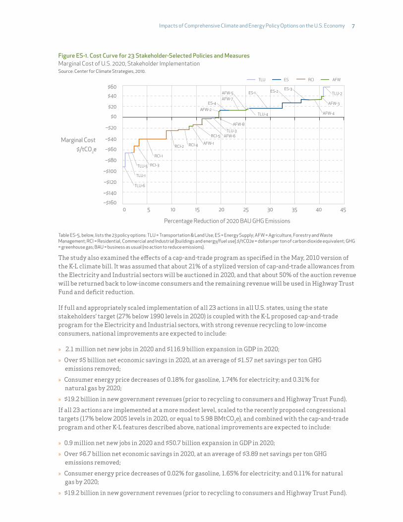
The cost curve of the 23 options in Figure ES-1 shows the GHG reduction potential (horizontal axis) as well as the cost or savings (positive for cost or negative for savings dollar figures on the vertical axis). See Table ES-5 for list of the names and the specific GHG reductions and costs or savings of the 23 actions. For example, Transportation and Land Use option 1 (TLU-1) is Vehicle Purchase Incentives, Including Rebates, and Energy Supply option 1 (ES-1) is a Renewable Portfolio Standard.
» Executive Summary
Impacts of Comprehensive Climate and Energy Policy Options on the U.S. Economy !7
Figure ES-1. Cost Curve for 23 Stakeholder-Selected Policies and Measures Marginal Cost of U.S. 2020, Stakeholder ImplementationSource: Center for Climate Strategies, 2010.
Marginal Cost $/tCO2e
Percentage Reduction of 2020 BAU GHG Emissions
–$1600 5 10 15 20 25 30 35 40 45
–$140
–$120
–$100
–$80
–$60
–$40
–$20
$0
$20
$40
$60
TLU-6
TLU-1
TLU-5
TLU-3
TLU-4
TLU-2
RCI-3
RCI-1
RCI-2 RCI-4 AFW-1
AFW-6
AFW-8
AFW-2
AFW-7AFW-5
AFW-3
AFW-4
ES-4
ES-1 ES-2 ES-3
RCI-5
TLU ES AFWRCI
Table ES-5, below, lists the 23 policy options: TLU = Transportation & Land Use; ES = Energy Supply; AFW = Agriculture, Forestry and Waste Management; RCI"="Residential, Commercial and Industrial [buildings and energy/fuel use].$/tCO2e = dollars per ton of carbon dioxide equivalent; GHG = greenhouse gas; BAU = business as usual (no action to reduce emissions). The study also examined the e!ects of a cap-and-trade program as specified in the May, 2010 version of the K-L climate bill. It was assumed that about 21% of a stylized version of cap-and-trade allowances from the Electricity and Industrial sectors will be auctioned in 2020, and that about 50% of the auction revenue will be returned back to low-income consumers and the remaining revenue will be used in Highway Trust Fund and deficit reduction.
If full and appropriately scaled implementation of all 23 actions in all U.S. states, using the state stakeholders’ target (27% below 1990 levels in 2020) is coupled with the K-L proposed cap-and-trade program for the Electricity and Industrial sectors, with strong revenue recycling to low-income consumers, national improvements are expected to include:
"» 2.1 million net new jobs in 2020 and $116.9 billion expansion in GDP in 2020;
"» Over $5 billion net economic savings in 2020, at an average of $1.57 net savings per ton GHG emissions removed;
"» Consumer energy price decreases of 0.18% for gasoline, 1.74% for electricity; and 0.31% for natural gas by 2020;
"» $19.2 billion in new government revenues (prior to recycling to consumers and Highway Trust Fund).
If all 23 actions are implemented at a more modest level, scaled to the recently proposed congressional targets (17% below 2005 levels in 2020, or equal to 5.98 BMtCO2e), and combined with the cap-and-trade program and other K-L features described above, national improvements are expected to include:
"» 0.9 million net new jobs in 2020 and $50.7 billion expansion in GDP in 2020;
"» Over $6.7 billion net economic savings in 2020, at an average of $3.89 net savings per ton GHG emissions removed;
"» Consumer energy price decreases of 0.02% for gasoline, 1.65% for electricity; and 0.11% for natural gas by 2020;
"» $19.2 billion in new government revenues (prior to recycling to consumers and Highway Trust Fund).

8! Johns Hopkins University and Center for Climate Strategies
This moderate implementation scenario does not perform as well economically as the full implementation scenarios because it does not provide the same level of cost-saving actions, or high employment and income stimulating actions, as the more aggressively targeted scenarios.
The 16 states on whose climate plans the work is based are: Alaska, Arkansas, Arizona, Colorado, Florida, Iowa, Maryland, Michigan, Minnesota, Montana, New Mexico, North Carolina, Pennsylvania, South Carolina, Vermont, and Washington. These were selected because they used consistent, transparent and formal procedures to develop and quantify measures, and they followed standard methodological guidelines that are peer reviewed and well accepted in practice. The selection, design, and specifications for analysis of these policy recommendations were made by stakeholders with facilitative and technical assistance by CCS.
To ensure that the results are consistent and current, the 16 state climate action plans were updated to account for recent federal and state actions, the e!ects of the recession, and more recent fuel price projections. Policy action results for the remaining 34 states were projected to national level implementation through customized extrapolation using 37 state and sector-specific characterizing factors and a method that estimates the scaled e!ects of state-level implementation and performance of each of the 23 policies. (See Section 2 and Annex A.*)
Recommended actions by state climate change stakeholders included policies and measures in all sectors, at all levels of government (under a national framework), and a variety of specific matching policy instruments (including price and non price approaches) needed for achieving GHG targets, economic and energy benefits. For instance, policy tools for the 23 actions selectively include targeted funding support, tax incentives, price incentives, reform of codes and standards, technical assistance, information and education, reporting and disclosure, and voluntary or negotiated agreements.
Analysis also shows the importance of integrating local, state and federal actions, as well as policy instruments, to minimize costs and maximize co-benefits. For example, as shown in Figure ES-2:
"» 38% of total potential emission reductions from these 23 options can be achieved through measures under shared federal and state jurisdiction;
"» 31% of potential emissions reductions can be achieved through measures primarily under state jurisdiction;
"» 31% of potential emissions reductions can be achieved through measures primarily under local or shared local/state jurisdiction.
Figure ES-2. State Government and Shared Responsibility for GHG Reductions 2020 Stakeholder Implementation Potential GHG Emissions Reductions by Jurisdiction Source: Center for Climate Strategies, 2010.
SharedState/Federal
38%
Primary State31%
SharedLocal/State
28%
Primary Local 3%
* The Annexes to this report are available at energypolicyreport.jhu.edu.

Impacts of Comprehensive Climate and Energy Policy Options on the U.S. Economy !9
Figure ES-3 indicates the potential GHG reductions from the 23 policies and measures showing the reductions based on the levels of government with key or shared responsibility.
Figure ES-3. GHG Reduction Potential of Stakeholder Policies by Level of Government U.S. 1990-2020 GHG Reduction Potential by Jurisdiction, Stakeholder ImplementationSource: Center for Climate Strategies, 2010.
MMtCO2e
0
19901992
19941996
19982000
20022004
20062008
20102012
20142016
20182020
1,000
2,000
3,000
4,000
5,000
6,000
7,000
8,000
1990 GHG Emissions Level
Shared State/Federal
Shared State/Local
Primary State
Primary Local
Gross Emissions(Consumption Basis excluding sinks)
MMtCO2e = million metric tons carbon dioxide equivalent; GHG = greenhouse gas.
The study underscores the strategic benefits of comprehensive approaches to managing GHG emissions and the need for a national framework to support a “balanced portfolio” of actions—one that takes actions across all sectors of the economy to find the most cost e!ective measures. It also underscores the importance of stakeholder involvement in policy development.
Figure ES-4 shows the potential emission reductions from multiple sectors of the economy using the state stakeholders’ target (27% below 1990 levels in 2020).
Figure ES-4. GHG Reduction Potential of Stakeholder Options by Sector U.S. 2020 GHG Reduction Potential by Sector, Stakeholder Implementation (Total from Individual Options)Source: Center for Climate Strategies, 2010.
MMtCO2e
0
19901992
19941996
19982000
20022004
20062008
20102012
20142016
20182020
1,000
2,000
3,000
4,000
5,000
6,000
7,000
8,000
1990 GHG Emissions Level
ES Reduction
RCI Reduction
TLU Reduction
AFW Reduction
Gross Emissions(Consumption Basis excluding sinks)
MMtCO2e = million metric tons carbon dioxide equivalent; GHG = greenhouse gas; ES = Energy Supply: RCI = Residential, Commercial and Industrial [buildings and energy/fuel use]; TLU"="Transportation & Land Use; AFW = Agriculture, Forestry and Waste Management.
10! Johns Hopkins University and Center for Climate Strategies
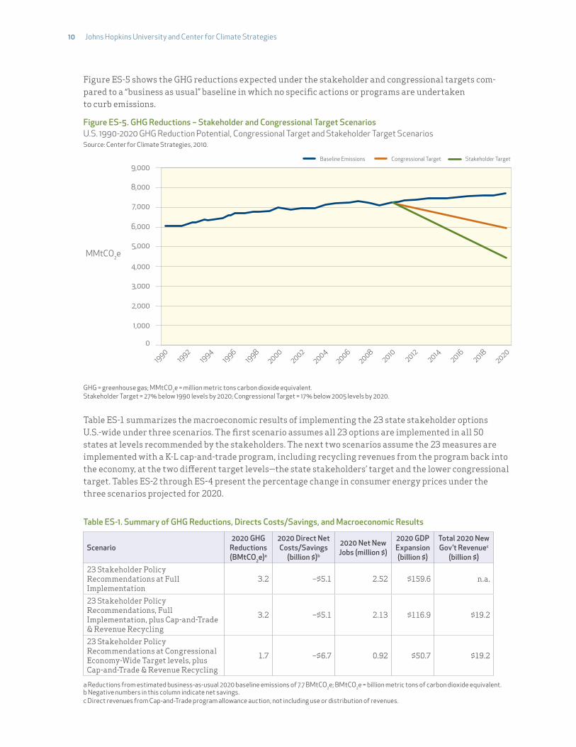
Figure ES-5 shows the GHG reductions expected under the stakeholder and congressional targets com-pared to a “business as usual” baseline in which no specific actions or programs are undertaken to curb emissions.
Figure ES-5. GHG Reductions – Stakeholder and Congressional Target Scenarios U.S. 1990-2020 GHG Reduction Potential, Congressional Target and Stakeholder Target ScenariosSource: Center for Climate Strategies, 2010.
MMtCO2e
0
19901992
19941996
19982000
20022004
20062008
20102012
20142016
20182020
1,000
2,000
3,000
4,000
5,000
6,000
7,000
8,000
9,000Baseline Emissions Stakeholder TargetCongressional Target
GHG = greenhouse gas; MMtCO2e = million metric tons carbon dioxide equivalent.Stakeholder Target = 27% below 1990 levels by 2020; Congressional Target = 17% below 2005 levels by 2020.
Table ES-1 summarizes the macroeconomic results of implementing the 23 state stakeholder options U.S.-wide under three scenarios. The first scenario assumes all 23 options are implemented in all 50 states at levels recommended by the stakeholders. The next two scenarios assume the 23 measures are implemented with a K-L cap-and-trade program, including recycling revenues from the program back into the economy, at the two di!erent target levels—the state stakeholders’ target and the lower congressional target. Tables ES-2 through ES-4 present the percentage change in consumer energy prices under the three scenarios projected for 2020.
Table ES-1. Summary of GHG Reductions, Directs Costs/Savings, and Macroeconomic Results
Scenario2020 GHG
Reductions (BMtCO2e)a
2020 Direct Net Costs/Savings
(billion $)b
2020 Net New Jobs (million $)
2020 GDP Expansion (billion $)
Total 2020 New Gov’t Revenuec
(billion $)23 Stakeholder Policy Recommendations at Full Implementation
3.2 –$5.1 2.52 $159.6 n.a.
23 Stakeholder Policy Recommendations, Full Implementation, plus Cap-and-Trade & Revenue Recycling
3.2 –$5.1 2.13 $116.9 $19.2
23 Stakeholder Policy Recommendations at Congressional Economy-Wide Target levels, plus Cap-and-Trade & Revenue Recycling
1.7 –$6.7 0.92 $50.7 $19.2
a Reductions from estimated business-as-usual 2020 baseline emissions of 7.7 BMtCO2e; BMtCO2e = billion metric tons of carbon dioxide equivalent. b Negative numbers in this column indicate net savings.c Direct revenues from Cap-and-Trade program allowance auction, not including use or distribution of revenues.

Impacts of Comprehensive Climate and Energy Policy Options on the U.S. Economy !11
REMI Results on Consumer Energy Prices for Year 2020 (percentage price change from baseline level)
Table ES-2. Scenario 1: Stakeholder Target Only
Energy Source Mitigation Activities (full implementation of the 23 super options)
Gasoline –0.56%
Electricity –2.01%
Natural Gas –0.87%
Table ES-3. Scenario 2: Stakeholder Target + C&T + Revenue Recycling
Energy Source
Mitigation Activities (full implementation
of the 23 super options)
Allowance Purchases
from Auction
Allowance Auction Revenue
Recycling
Sectoral Trading — Allowance Purchases
Sectoral Trading — Allowance
Sales
International O"set
PurchasesTotal
Gasoline –0.56% 0.27% 0.01% 0.06% –0.07% 0.11% –0.18%
Electricity –2.01% 0.20% 0.01% 0.04% –0.06% 0.08% –1.74%
Natural Gas –0.87% 0.50% 0.01% 0.04% –0.06% 0.07% –0.31%
Table ES-4. Scenario 3: Congressional Target + C&T + Revenue Recycling
Energy Source
Mitigation Activities (scale-back
implementation of the 23 super options)
Allowance Purchases
from Auction
Allowance Auction Revenue
Recycling
Sectoral Trading — Allowance Purchases
Sectoral Trading — Allowance
Sales
Total
Gasoline –0.35% 0.29% 0.01% 0.15% –0.12% –0.02%
Electricity –1.25% 0.21% 0.01% 0.11% –0.73% –1.65%
Natural Gas –0.55% 0.60% 0.01% 0.10% –0.27% –0.11%
Table ES-5 presents a listing of the 23 stakeholder-selected policies showing the annual GHG reductions each is projected to achieve in 2020 if implemented nationwide. Each option’s costs or cost savings and macroeconomic impacts (net employment and gross domestic product estimates) are also shown. Table ES-6 presents the same information for the 23 options combined with a cap-and-trade program, revenue recycling, and lower target embodied in the K-L legislation.

12! Johns Hopkins University and Center for Climate Strategies
Table ES-5. Impacts of 23 Stakeholder-Recommended, Sector-Based Climate and Energy Policy Options on the U.S. Economy – Fully Implemented Stakeholder Proposals Plus Cap-and-Trade and Revenue Recycling
Sector Climate Mitigation Actions
2020 Annual GHG Reduction (MMtCO2e)
Cost or Cost Savings per
Ton GHG Removed ($)
2020 Annual Cost or Cost
Savings (million $)
2020 Net Employment
Impact (thousands)
2020 GDP Impact
(billion $)
Impact on GDP 2010–2020 NPV (billion $)
AFW–1 Crop Production Practices to Achieve GHG Benefits 65.01 –$15.69 –$1,020 87.7 $4.55 $17.50
AFW–2 Livestock Manure – Anaerobic Digestion and Methane Utilization 19.25 $11.27 $217 –0.9 –$0.17 –$0.58
AFW–3 Forest Retention 39.21 $39.38 $1,544 71.2 $0.48 $3.45
AFW–4 Reforestation/A!orestation 178.77 $33.18 $5,932 –117.8 –$11.07 –$73.47
AFW–5 Urban Forestry 39.96 $15.35 $613 505.3 $5.44 $40.12
AFW–6 MSW Source Reduction 147.09 –$3.20 –$471 25.7 $2.53 $10.37
AFW–7 Enhanced Recycling of Municipal Solid Waste 249.27 $13.39 $3,339 114.4 $10.38 $51.61
AFW–8 Landfill Gas Management 48.38 $0.34 $17 94 $10.44 $26.47
Agriculture, Forestry, Waste Management (AFW) Totals 786.96 $12.92 $10,170 779.6 $22.58 $75.46
ES–1 Renewable Portfolio Std. 508.39 $17.84 $9,071 –58.6 –$5.35 –$35.52
ES–2 Nuclear 300.77 $26.98 $8,116 –73.3 –$6.85 –$8.14
ES–3 Carbon Capture Sequestration/Reuse 130.23 $32.92 $4,287 –35.4 –$4.47 –$16.57
ES–4 Coal Plant E$ciency Improvements and Repowering 151.05 $12.95 $1,956 1.1 $0.48 $0.86
Energy Supply (ES) Totals 1,090.45 $21.49 $23,430 –166.2 –$16.19 –$59.38
RCI–1 Demand Side Management Programs 424.80 –$40.71 –$17,293 886.2 $90.05 $305.05
RCI–2 High Performance Buildings (Private and Public) 193.88 –$24.99 –$4,845 183.3 $12.12 $40.14
RCI–3 Appliance standards 80.86 –$53.21 –$4,302 25.1 $0.05 –$0.43
RCI–4 Building Codes 161.08 –$22.86 –$3,682 181.1 $13.65 $49.05
RCI–5 Combined Heat and Power 136.37 –$13.18 –$1,798 –127.9 –$21.17 –$104.38
Residential, Commercial and Industrial (RCI) Totals 996.98 –$32.02 –$31,920 1,147.80 $94.70 $289.44
TLU–1 Vehicle Purchase Incentives, Including Rebates 103.07 –$66.37 –$6,841 179.5 $16.51 $39.64
TLU–2 Renewable Fuel Standard (Biofuels Goals) 92.34 $57.14 $5,277 –25.2 –$4.78 –$17.08
TLU–3 Smart Growth/Land Use 71.04 –$1.11 –$79 165.7 $6.15 $19.54
TLU–4 Transit 27.05 $16.72 $452 52.2 $1.18 $2.46
TLU–5 Anti–Idling Technologies and Practices 33.82 –$65.19 –$2,205 16.7 $1.92 $2.96
TLU–6 Mode Shi# - Truck to Rail 36.85 –$91.56 –$3,374 40.9 $6.69 $2.92
Transportation and Land Use (TLU) Totals 364.17 –$18.59 –$6,770 429.8 $27.68 $50.44
23 Policy Totals (summation) 3,238.57 –$1.57 –$5,090 2,191 $128.77 $355.97
Stakeholder Recommendations Scenario Results (simultaneous) 3,238.57 –$1.57 –$5,090 2,524 $159.60 $406.74
Stakeholder Recommendations w/Cap & Trade + Revenue Recycling 3,238.57 –$1.57 –$5,090 2,132 $116.90 n.a.
GHG = greenhouse gas; MMtCO2e = million metric tons carbon dioxide equivalent; GDP = gross domestic product: MSW = municipal solid waste; NPV = net present value. Negative numbers indicate cost savings.Note: The 23 Policy Totals are a simple summation of each policy’s estimated results; interactions and double counting between policies have been accounted for in individual policy results; the Stakeholder Scenario simultaneous results of the REMI analysis take into account the interactive economic e#ects of policies.
Impacts of Comprehensive Climate and Energy Policy Options on the U.S. Economy !13
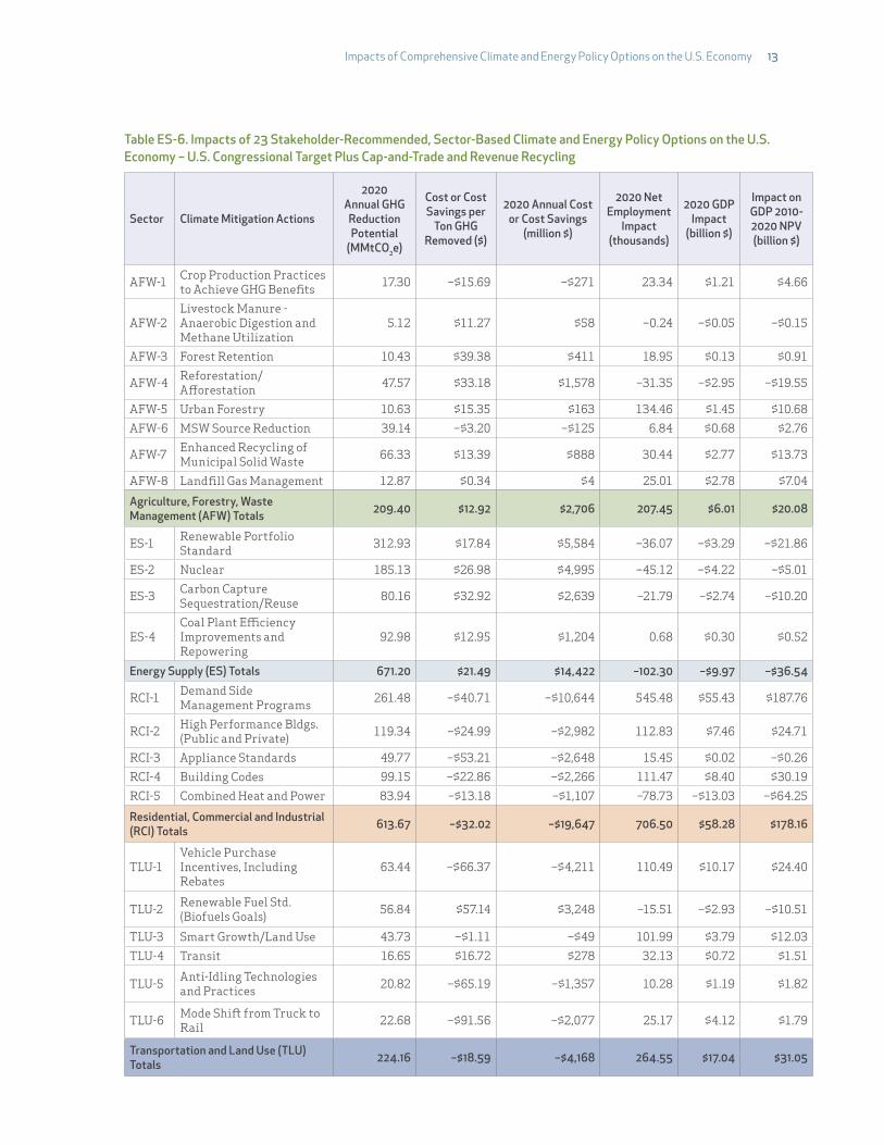
Table ES-6. Impacts of 23 Stakeholder-Recommended, Sector-Based Climate and Energy Policy Options on the U.S. Economy – U.S. Congressional Target Plus Cap-and-Trade and Revenue Recycling
Sector Climate Mitigation Actions
2020 Annual GHG Reduction Potential
(MMtCO2e)
Cost or Cost Savings per
Ton GHG Removed ($)
2020 Annual Cost or Cost Savings
(million $)
2020 Net Employment
Impact (thousands)
2020 GDP Impact
(billion $)
Impact on GDP 2010-2020 NPV (billion $)
AFW-1 Crop Production Practices to Achieve GHG Benefits 17.30 –$15.69 –$271 23.34 $1.21 $4.66
AFW-2Livestock Manure - Anaerobic Digestion and Methane Utilization
5.12 $11.27 $58 –0.24 –$0.05 –$0.15
AFW-3 Forest Retention 10.43 $39.38 $411 18.95 $0.13 $0.91
AFW-4 Reforestation/A!orestation 47.57 $33.18 $1,578 –31.35 –$2.95 –$19.55
AFW-5 Urban Forestry 10.63 $15.35 $163 134.46 $1.45 $10.68
AFW-6 MSW Source Reduction 39.14 –$3.20 –$125 6.84 $0.68 $2.76
AFW-7 Enhanced Recycling of Municipal Solid Waste 66.33 $13.39 $888 30.44 $2.77 $13.73
AFW-8 Landfill Gas Management 12.87 $0.34 $4 25.01 $2.78 $7.04
Agriculture, Forestry, Waste Management (AFW) Totals 209.40 $12.92 $2,706 207.45 $6.01 $20.08
ES-1 Renewable Portfolio Standard 312.93 $17.84 $5,584 –36.07 –$3.29 –$21.86
ES-2 Nuclear 185.13 $26.98 $4,995 –45.12 –$4.22 –$5.01
ES-3 Carbon Capture Sequestration/Reuse 80.16 $32.92 $2,639 –21.79 –$2.74 –$10.20
ES-4Coal Plant E$ciency Improvements and Repowering
92.98 $12.95 $1,204 0.68 $0.30 $0.52
Energy Supply (ES) Totals 671.20 $21.49 $14,422 –102.30 –$9.97 –$36.54
RCI-1 Demand Side Management Programs 261.48 –$40.71 –$10,644 545.48 $55.43 $187.76
RCI-2 High Performance Bldgs. (Public and Private) 119.34 –$24.99 –$2,982 112.83 $7.46 $24.71
RCI-3 Appliance Standards 49.77 –$53.21 –$2,648 15.45 $0.02 –$0.26
RCI-4 Building Codes 99.15 –$22.86 –$2,266 111.47 $8.40 $30.19
RCI-5 Combined Heat and Power 83.94 –$13.18 –$1,107 –78.73 –$13.03 –$64.25
Residential, Commercial and Industrial (RCI) Totals 613.67 –$32.02 –$19,647 706.50 $58.28 $178.16
TLU-1Vehicle Purchase Incentives, Including Rebates
63.44 –$66.37 –$4,211 110.49 $10.17 $24.40
TLU-2 Renewable Fuel Std. (Biofuels Goals) 56.84 $57.14 $3,248 –15.51 –$2.93 –$10.51
TLU-3 Smart Growth/Land Use 43.73 –$1.11 –$49 101.99 $3.79 $12.03
TLU-4 Transit 16.65 $16.72 $278 32.13 $0.72 $1.51
TLU-5 Anti-Idling Technologies and Practices 20.82 –$65.19 –$1,357 10.28 $1.19 $1.82
TLU-6 Mode Shi# from Truck to Rail 22.68 –$91.56 –$2,077 25.17 $4.12 $1.79
Transportation and Land Use (TLU) Totals 224.16 –$18.59 –$4,168 264.55 $17.04 $31.05
14! Johns Hopkins University and Center for Climate Strategies
Sector Climate Mitigation Actions
2020 Annual GHG Reduction Potential
(MMtCO2e)
Cost or Cost Savings per
Ton GHG Removed ($)
2020 Annual Cost or Cost Savings
(million $)
2020 Net Employment
Impact (thousands)
2020 GDP Impact
(billion $)
Impact on GDP 2010-2020 NPV (billion $)
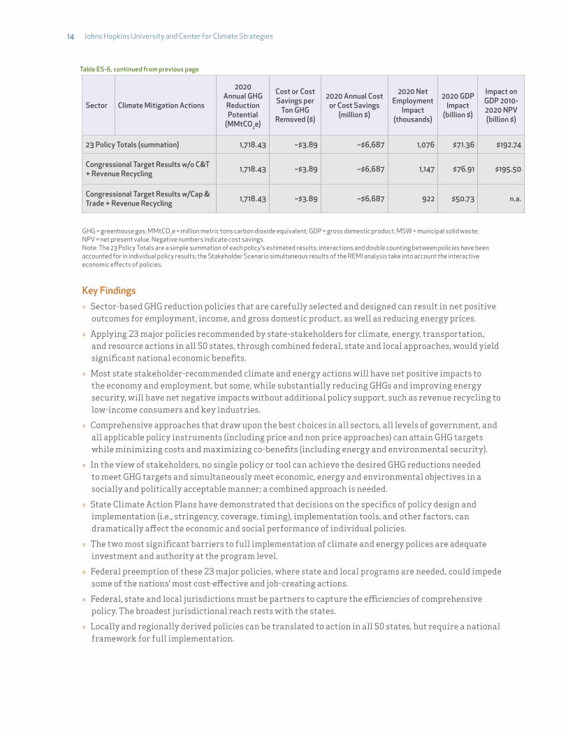
23 Policy Totals (summation) 1,718.43 –$3.89 –$6,687 1,076 $71.36 $192.74
Congressional Target Results w/o C&T + Revenue Recycling 1,718.43 –$3.89 –$6,687 1,147 $76.91 $195.50
Congressional Target Results w/Cap & Trade + Revenue Recycling 1,718.43 –$3.89 –$6,687 922 $50.73 n.a.
GHG = greenhouse gas; MMtCO2e = million metric tons carbon dioxide equivalent; GDP = gross domestic product; MSW = municipal solid waste; NPV = net present value. Negative numbers indicate cost savings.Note: The 23 Policy Totals are a simple summation of each policy’s estimated results; interactions and double counting between policies have been accounted for in individual policy results; the Stakeholder Scenario simultaneous results of the REMI analysis take into account the interactive economic e#ects of policies.
Key Findings"» Sector-based GHG reduction policies that are carefully selected and designed can result in net positive
outcomes for employment, income, and gross domestic product, as well as reducing energy prices.
"» Applying 23 major policies recommended by state-stakeholders for climate, energy, transportation, and resource actions in all 50 states, through combined federal, state and local approaches, would yield significant national economic benefits.
"» Most state stakeholder-recommended climate and energy actions will have net positive impacts to the economy and employment, but some, while substantially reducing GHGs and improving energy security, will have net negative impacts without additional policy support, such as revenue recycling to low-income consumers and key industries.
"» Comprehensive approaches that draw upon the best choices in all sectors, all levels of government, and all applicable policy instruments (including price and non price approaches) can a"ain GHG targets while minimizing costs and maximizing co-benefits (including energy and environmental security).
"» In the view of stakeholders, no single policy or tool can achieve the desired GHG reductions needed to meet GHG targets and simultaneously meet economic, energy and environmental objectives in a socially and politically acceptable manner; a combined approach is needed.
"» State Climate Action Plans have demonstrated that decisions on the specifics of policy design and implementation (i.e., stringency, coverage, timing), implementation tools, and other factors, can dramatically a!ect the economic and social performance of individual policies.
"» The two most significant barriers to full implementation of climate and energy polices are adequate investment and authority at the program level.
"» Federal preemption of these 23 major policies, where state and local programs are needed, could impede some of the nations’ most cost-e!ective and job-creating actions.
"» Federal, state and local jurisdictions must be partners to capture the e$ciencies of comprehensive policy. The broadest jurisdictional reach rests with the states.
"» Locally and regionally derived policies can be translated to action in all 50 states, but require a national framework for full implementation.
Table ES-6, continued from previous page

Impacts of Comprehensive Climate and Energy Policy Options on the U.S. Economy !15
"» If caps and taxes are combined with appropriate sector-based policies and measures, their cost will be significantly lower and their co-benefits will be higher than if they are implemented alone.
"» Auctions of allowances in key sectors will have negative impacts on economic performance if funds are not recycled e!ectively. However, reinvestment to targeted support for low-income consumers and key industries can significantly reverse these impacts.
"» Policy strategies applicable to the next decade must be combined with longer term policies to address future decades, and provide an important transition.
16! Johns Hopkins University and Center for Climate Strategies
%&'()*+ *+&
» IntroductionAs Congress si#s through the complex programmatic, economic, environmental, political, jurisdictional, and equity issues associated with national climate policy, the work already done by the states and their stakeholders can provide critical policy and analytical guidance. Since 2000, 34 U.S. states have completed or are developing comprehensive greenhouse gas (GHG) reduction plans that identify, design, evaluate and recommend specific policy options for application at the local, state and federal levels to achieve climate change stabilization targets and important co-benefits such as economic growth and energy security.
This growing database of state-level stakeholder-recommended GHG reduction measures presents an opportunity to model the potential for national application of similar policies and measures, including the GHG reduction potential and cost e!ectiveness of each measure. This report presents the methods, findings and conclusions of this research, and carries the investigation two steps further; in addition to projecting the performance of successful state-level climate policies on a national scale, the authors have examined the likely impact of national climate policy implementation on U.S. employment, gross domestic product, incomes and consumer energy prices; and second, analysis of the Kerry-Lieberman (K-L) bill using the national data developed above.
The three modeling scenarios presented here are intended to o!er Congressional leaders highly relevant information. The first two scenarios demonstrate the potential for full implementation of stakeholder recommended policies and measures. The third, Scenario 3, reflects the application of the stakeholder-recommended measures using the framework of the K-L bill. Like Scenario 2, this scenario incorporates a limited national cap-and-trade program modeled on the bill and utilizes the K-L GHG reduction targets and other features, but it limits application of the sector-based policies and measures to levels equal to congressional economy-wide targets.
The results of this study reflect what the authors believe to be the best estimation of GHG reduction opportunities, direct costs and savings, and indirect or macroeconomic impacts on a national level. The analysis is constructed from the bo"om-up and is based upon policy measures selected, designed and recommended by diverse stakeholders from every region in the U.S. Furthermore, key analytical methods used in this study were subjected to external review.
These state climate plans were the product of thousands of formal, intensive stakeholder deliberations, and represent what is politically achievable and institutionally feasible. Stakeholders were tasked not only to meet GHG reduction goals, but other objectives such as cost containment, economic growth and job creation, energy security, improved public health outcomes, equity issues, and a range of policy implementation feasibility constraints.
The results of state climate action plans in the U.S. have varied from state to state and over time, and include many similar and overlapping recommendations and findings. But the fundamental approaches to policy development and analysis have been consistent for the 16 states that retained the Center for Climate Strategies (CCS) for facilitation and technical assistance, whose results are part of this study. Today, over 1,000 specific policy options have been designed and analyzed for these state action plans and converted to microeconomic or cost e!ectiveness analysis.
For macroeconomic analysis of state climate action plans, and for national macroeconomic analysis, a linked modeling system that integrates microeconomic and macroeconomic models was developed.

Impacts of Comprehensive Climate and Energy Policy Options on the U.S. Economy !17
The national macroeconomic analysis of climate policy measures uses the Regional Economic Models, Inc. (REMI) Policy Insight tool, in combination with this cost e!ectiveness database from state climate plans, to model the macroeconmic impacts of 23 major policies and measures recommended by state stakeholders.
The authors and their associates previously conducted six macroeconomic analyses1 of state climate action plans. These studies used state-of-the-art econometric models to estimate the impact of the stakeholder-recommended climate policies on jobs, income, gross domestic product, and consumer energy prices. The Florida study was successfully submi"ed for peer review. Due to the confluence of economic, energy and climate change related concerns of the public and the policy community, this information has been in great demand by governors, policy makers and legislators as they contemplate the best ways to advance climate and clean energy plans into rule, law or program.
This report contains an Executive Summary that presents key findings and results of this work. Available online at energypolicyreport.jhu.edu are a series of Annexes that contain significant detail concerning the data sources, methods used and assumptions employed in this research, including illustrative examples of calculations. The report sections that follow provide an overview of the detail found in the Annexes and the findings and results of the study.
Section 2 National Scale-up of State Actions: Greenhouse Gas Reduction Potential and Microeconomic Analysis of Mitigation Options, presents the approach used to document, update and extrapolate the analysis of state climate action plan results to the national scale. Findings reflect the direct cost or savings resulting from the implementation of the GHG reduction policies and projections of GHG reduction potential for the policies, both individually and in the aggregate, under three national implementation scenarios.
Section 3 Macroeconomic E!ects of Mitigation Options: REMI Model Analysis, presents the expected macroeconomic impacts of policy implementation at the national level. As noted above, the model used in this analysis is the Regional Economic Models, Inc. Policy Insight Plus (PI+), which is described in detail in Annex C.*
Section 4 Mitigation Option Implementation: Jurisdictional and Programmatic Issues, examines the practical realities of local, state and federal jurisdictional authority over highly diverse climate mitigation policies that a!ect all sectors of the economy. This section o!ers some insight for policy makers at all three government levels regarding apparent prerequisites for successful comprehensive climate policy implementation.
Section 5 Conclusions, o!ers what the authors see as the key insights provided by this work. Until recently the major focus of state climate plans has been on the direct impacts of individual mitigation options. However, the indirect or macroeconomic impacts of climate and energy policies are o#en of greater interest to policy makers as political decisions are made. This section pinpoints key issues, impacts and dynamics of the economy to be considered and addressed in the national policy formulation process, and the value of sub national guidance.
1. North Carolina, Arizona, Florida, Michigan, Pennsylvania, and Wisconsin.* The Annexes to this report are available at energypolicyreport.jhu.edu.

18! Johns Hopkins University and Center for Climate Strategies
%&'()*+ (,*
» National Scale-up of State Actions: GHG Reduction Potential and Microeconomic Analysis of Climate Mitigation Options
Over the last 6 years the Center for Climate Strategies (CCS) has facilitated and provided technical support for the development of climate action plans through a sequential fact-finding and consensus building process for 24 U.S. states. The identification, design and analysis of policy option recommendations in the states’ action planning processes involved preliminary fact finding that included the development of a dra# inventory and forecast of greenhouse gas (GHG) emissions for each state engaged in plan development, plus a dra# inventory and catalog of existing and planned emissions-reduction actions, combined with actions considered or undertaken in other U.S. states (over 300 actions in all sectors). Next, stakeholder advisory groups engaged in joint fact-finding and policy development processes that involved the following sequential steps and stakeholder decisions:
1.-Development of a preliminary inventory and forecast of GHG emissions, and a full range of potential options in the form of a catalog of states’ actions, including actions from other states’ climate action planning as well as the state in question.
2.-Expansion of the initial states’ catalog of actions to fill gaps and provide a full range of potential actions of relevance to the state.
3.-Narrowing of the catalog of actions to a set of top ten or so dra# policy options for each sector, based on screening criteria that included: GHG reduction potential, cost-e!ectiveness, co-benefits or costs, and feasibility considerations.
4.-Development of dra# policy design parameters for each individual policy option (timing, level of e!ort, coverage of implementing parties, etc.).
5.-Modifications of inventory and forecast estimates if/as needed.
6.-Identification of preferred data sources, methods, and assumptions for analysis of individual policy options, including overarching policies and guidelines, as well as common assumptions and guidelines for each sector.
7.-Identification of preferred or potentially applicable policy implementation tools for individual policy options.
8.-Development of estimated GHG reduction potential and costs/savings per metric ton of GHG removed for specific individual policy options.
9.-Identification and qualitative or quantitative assessment of co-benefits and costs for specific individual policy options.
10.-Development of estimated GHG reduction potential and costs or savings per metric ton of GHG removed for all policy options combined (aggregate, system wide analysis).
11.-Final approval of individual policy option recommendations and related planning goals based on iterative feedback and consensus building.
12.-Development of final report language.
13.-Transmi"al of the final report to the convening body, typically the Governor’s o$ce.

Impacts of Comprehensive Climate and Energy Policy Options on the U.S. Economy !19
This work with the 24 states has identified more than 1,000 specific policy options that have been considered by the various states. However, due to the limitations of this project, the authors could not reanalyze all of these policy options, and the policy community needed a streamlined understanding of policy solutions for national application. As a result, a list of 23 so-called “super options” was proposed and evaluated, following review and approval by the 18 governors’ o$ces of the Southern Governors’ Association (SGA).1 These super options are actually categories or groupings of more specific policies that have been or could be implemented at the federal, state or local level. They were chosen because they typically (1) have the greatest GHG reduction potential; (2) are commonly recommended gateway options, sometimes with limited near-term reduction potential but holding great promise in later years (carbon capture and storage or reuse, nuclear); or (3) are highly cost-e!ective and important and commonly recommended for other reasons (e.g., state lead by example).
Table 2-1. 23 Climate Policy “Super Options” by Sector
Agriculture, Forestry and Waste
AFW-1 Crop Production Practices to Achieve GHG Benefits
AFW-2 Livestock Manure—Anaerobic Digestion and Methane Utilization
AFW-3 Forest Retention
AFW-4 Reforestation/A!orestation
AFW-5 Urban Forestry
AFW-6 Municipal Solid Waste Source Reduction
AFW-7 Enhanced Recycling of Municipal Solid Waste
AFW-8 MSW Landfill Gas Management
Energy Supply
ES-1 Renewable Portfolio Standard
ES-2 Nuclear
ES-3 Carbon Capture Storage and Reuse, also known as Geologic Sequestration
ES-4 Coal Plant E$ciency Improvements and Repowering
Residential, Commercial and Industrial
RCI-1 Demand Side Management Programs
RCI-2 High-Performance Buildings (Private and Public Sector)
RCI-3 Appliance Standards
RCI-4 Building Codes
RCI-5 Combined Heat and Power
Transportation and Land Use
TLU-1 Vehicle Purchase Incentives, Including Rebates
TLU-2 Renewable Fuel Standard (Biofuels Goals)
TLU-3 Smart Growth/Land Use
TLU-4 Transit
TLU-5 Anti-Idling Technologies and Practices
TLU-6 Mode Shi# from Truck to Rail
CCSR = carbon capture and storage or reuse; GHG = greenhouse gas; MSW = municipal solid waste.
1. This national scale-up project is in part an outgrowth of work CCS performed for the SGA. The ve$ing of the 23 super options through those governors’ o%ces was performed as part of that e#ort. The final SGA report can be found at h$p://www.climatestrategies.us/template.cfm?FrontID=6081.

20! Johns Hopkins University and Center for Climate Strategies
These 23 “super options” were found to be responsible for approximately 90% of the total GHG emissions reductions potential of all the quantified options the state plans. Annex B* contains brief description of each super option by sector.
Because each state process was conducted independently and focused on individual state needs, and because they were stakeholder-driven and conducted at di!erent times over the past few years, di!erences exist between their specific choices on policy portfolios, policy designs, analytical specifications, prioritized final outcomes, and results. But the states’ plans also share many common issues and characteristics, therefore the results also overlap substantially in key policy areas. A#er reviewing the plans of all candidate states, 16 states’ results were chosen to serve as the base for this study.2 These 16 states are Alaska, Arkansas, Arizona, Colorado, Florida, Iowa, Maryland, Michigan, Minnesota, Montana, North Carolina, New Mexico, Pennsylvania, South Carolina, Vermont, and Washington. These states were deemed to have the most complete and methodologically consistent policy recommendation results and o!ered excellent geographic, climatological, economic, and demographic diversity.
To ensure consistency of analytical methods, assumptions and data sources across all 23 super options in all 16 state plans, the policy-level results of the state plans were individually updated using methods that addressed:
"» The e!ects of the recession and changes in future economic growth forecasts on projected levels of economic growth and other economy-driven assumptions;
"» The e!ects of changes in energy price forecasts; and
"» The impacts of recent state or federal actions on projected future levels of GHG emissions in the absence of the proposed new GHG reduction policies.
The updated results for GHG reductions and the cost-e!ectiveness of the mitigation options in the 16 states were utilized to extrapolate the results to the remaining states in the U.S. The 50-state data were then aggregated to determine the GHG reduction potential and direct cost or cost savings resulting from national implementation of the policies under three scenarios. This work served as the basis of the national marginal abatement cost curve development and the subsequent macroeconomic analysis.
For most policies, the modeling of policy performance in the 34 states without climate plans was conducted on a policy by policy basis using 37 published factors in order to capture state and sector-specific characteristics that would a!ect application of the standard set of 23 options to new geographical areas. These factors enabled the use of a ‘weighted average’ of the 16 states’ results to serve as the basis for the extrapolation. These 37 factor-based weighted averages were recalculated for each of the 23 super options, allowing sector and policy-level distinctions to be captured and reflected. Most of the transportation policies were modeled with the assistance of the U.S. Department of Energy VISION Model. Please refer to Annex A* for a detailed discussion of the methodology used in the extrapolation process.
2. California was not a state where CCS facilitated a stakeholder planning process and provided analysis, however a similar plan was developed there. The authors used partial results from the California plan where the analytical methods and assumptions were consistent with other states’ methods.* The Annexes to this report are available at energypolicyreport.jhu.edu.
Impacts of Comprehensive Climate and Energy Policy Options on the U.S. Economy !21
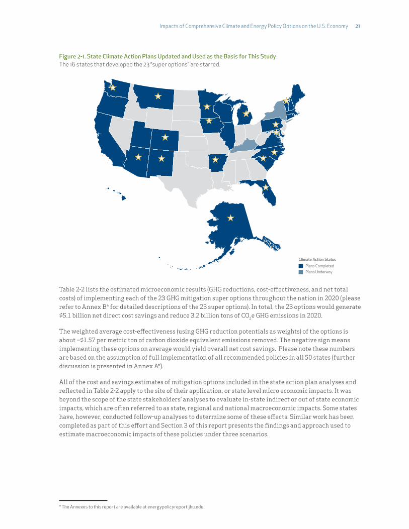
Figure 2-1. State Climate Action Plans Updated and Used as the Basis for This Study The 16 states that developed the 23 “super options” are starred.
Plans CompletedClimate Action Status
Plans Underway
Table 2-2 lists the estimated microeconomic results (GHG reductions, cost-e!ectiveness, and net total costs) of implementing each of the 23 GHG mitigation super options throughout the nation in 2020 (please refer to Annex B* for detailed descriptions of the 23 super options). In total, the 23 options would generate $5.1 billion net direct cost savings and reduce 3.2 billion tons of CO2e GHG emissions in 2020.
The weighted average cost-e!ectiveness (using GHG reduction potentials as weights) of the options is about –$1.57 per metric ton of carbon dioxide equivalent emissions removed. The negative sign means implementing these options on average would yield overall net cost savings. Please note these numbers are based on the assumption of full implementation of all recommended policies in all 50 states (further discussion is presented in Annex A*).
All of the cost and savings estimates of mitigation options included in the state action plan analyses and reflected in Table 2-2 apply to the site of their application, or state level micro economic impacts. It was beyond the scope of the state stakeholders’ analyses to evaluate in-state indirect or out of state economic impacts, which are o#en referred to as state, regional and national macroeconomic impacts. Some states have, however, conducted follow-up analyses to determine some of these e!ects. Similar work has been completed as part of this e!ort and Section 3 of this report presents the findings and approach used to estimate macroeconomic impacts of these policies under three scenarios.
* The Annexes to this report are available at energypolicyreport.jhu.edu.

22! Johns Hopkins University and Center for Climate Strategies
Table 2-2. Estimated GHG Reductions and Costs/Savings of the 23 GHG Mitigation Super Options
Sector Climate Mitigation Actions2020 Annual
GHG Reduction (MMtCO2e)
Cost or Cost Savings per Ton
GHG Removed ($)
2020 Annual Cost or Cost Savings
(million $)AFW–1 Crop Production Practices to Achieve GHG Benefits 65.01 –$15.69 –$1,020
AFW–2 Livestock Manure—Anaerobic Digestion and Methane Utilization 19.25 $11.27 $217
AFW–3 Forest Retention 39.21 $39.38 $1,544
AFW–4 Reforestation/A!orestation 178.77 $33.18 $5,932
AFW–5 Urban Forestry 39.96 $15.35 $613
AFW–6 MSW Source Reduction 147.09 –$3.20 –$471
AFW–7 Enhanced Recycling of Municipal Solid Waste 249.27 $13.39 $3,339
AFW–8 Landfill Gas Management 48.38 $0.34 $17
Agriculture, Forestry, Waste Management (AFW) Totals 786.96 $12.76# $10,170ES–1 Renewable Portfolio Standard 508.39 $17.84 $9,071
ES–2 Nuclear 300.77 $26.98 $8,116
ES–3 Carbon Capture Sequestration/Reuse 130.23 $32.92 $4,287
ES–4 Coal Plant E$ciency Improvements and Repowering 151.05 $12.95 $1,956
Energy Supply (ES) Totals 1,090.45# #$21.49 $23,430RCI–1 Demand Side Management Programs 424.80 –$40.71 –$17,293
RCI–2 High-Performance Buildings (Private and Public) 193.88 –$24.99 –$4,845
RCI–3 Appliance Standards 80.86 –$53.21 –$4,302
RCI–4 Building Codes 161.08 –$22.86 –$3,682
RCI–5 Combined Heat and Power 136.37 –$13.18 –$1,798
Residential, Commercial and Industrial (RCI) Totals 996.98# #–$32.02 –$31,919TLU–1 Vehicle Purchase Incentives, Including Rebates 103.07 –$66.37 –$6,841
TLU–2 Renewable Fuel Standard (Biofuels Goals) 92.34 $57.14 $5,277
TLU–3 Smart Growth/Land Use 71.04 –$1.11 –$79
TLU–4 Transit 27.05 $16.72 $452
TLU–5 Anti–Idling Technologies and Practices 33.82 –$65.19 –$2,205
TLU–6 Mode Shi#—Truck to Rail 36.85 –$91.56 –$3,374
Transportation and Land Use (TLU) Totals 364.17 –$18.59 –$6,771
23 Policy Totals 3,238.56 –$1.57 –$5,090
GHG = greenhouse gas; MMtCO2e = million metric tons carbon dioxide equivalent.Note: Positive numbers in the table represent net positive costs; negative numbers represent net negative costs, i.e., net savings.
The first scenario of analysis for the study modeled the policy options shown above; full implementation of all 23 super options in all 50 states. This scenario most directly reflects the full potential of the stakeholder recommendations and agreements. The second scenario models the same program with the added feature of a limited cap-and-trade program operating in the Electric Generation and Industrial sectors consistent with current congressional legislative proposals. The third scenario scales back the implementation of the 23 super options to exactly meet President Obama’s and congressional goal of 17% below 2005 levels in 2020, or equal to 5.98 billion metric tons carbon dioxide equivalent (BMtCO2e), and incorporates the same programmatic features as the second scenario. This third scenario most closely models the current congressional legislative plan for a national program.
The national GHG reduction potential and direct costs and savings of the 23 super options fully implemented (with or without the cap-and-trade) are graphically presented in Figures 2-2 and 2-3.
Figure 2-2 shows the national GHG reduction potential of the 23 options in ascending order. The options with the greatest GHG reduction potential in 2020 are the Renewable Portfolio Standard, Demand Side Management Programs and Nuclear energy. It is important to note that the reduction potential is

Impacts of Comprehensive Climate and Energy Policy Options on the U.S. Economy !23
dependent on the stringency or aggressiveness of the policy design. This analysis is based upon state-specific policies designed by stakeholders in up to 16 states. Within this sample there is some diversity of program design, as each option is tailored to the opportunities, needs and desires of each state. The scale-up methodology captures this diversity and applies the 16-state plan results on a weighted-average basis to each of the remaining states. The national stringency of each of these options therefore reflects a weighted average blend of the stakeholder-recommended policy designs found within those state climate action plans.
Figure 2-2. 2020 Reduction Potential of Super Options, Stakeholder Implementation
MMtCO2e
0
Livestock Manure
Transit
Anti-Idlin
g Techologies and Practices
Mode Shi! from Truck to Rail
Forest Retention
Urban Forestry
MSW Landfill Gas M
anagement
Crop Production Practices
Smart Growth/Land Use
Appliance Standards
Renewable Fuel Standard
Vehicle Purchase IncentivesCCSR
Combined Heat and Power
MSW Source Reduction
Coal Plant E"
ciency Improvements
Building Codes
Reforestation/A#orestation
High Performance Buildings
Enhanced Recycling of M
SW
Nuclear
Demand Side Management Programs
Renewable Portfolio Standard
100.00
200.00
300.00
400.00
500.00
600.00
ES RCI AFW TLU
MMtCO2e = million metric tons carbon dioxide equivalent; GHG = greenhouse gas; BAU = business as usual (no action to reduce emissions); CCSR = carbon capture and storage or reuse; TLU = Transportation and Land Use; ES = Energy Supply; AFW = Agriculture, Forestry, and Waste Management; RCI"="Residential, Commercial, and Industrial [buildings and energy/fuel use].
Figure 2-3 ranks the 23 super options in ascending order of marginal cost e!ectiveness, measured in net dollars per ton of carbon dioxide equivalent ($/tCO2e) avoided or removed. Note that the bars to the le# fall below the $0 line. These negative cost options represent a net direct savings, while those options having bars that reach above the $0 line have a net direct cost. Direct cost and savings indicate the cost or savings to society, and not to any particular entity. For example, the most cost e!ective policy is Mode Shi# from Truck to Rail, with an expected net cost of –$91 (or a $91 savings). The railroad freight industry clearly stands to benefit from this policy but the trucking industry and the diesel fuel refiners, distributors and retailers will lose business. Overall, however, the net impact to society as represented by the broader economy represents a significant overall savings.

24! Johns Hopkins University and Center for Climate Strategies
Figure 2-3. Cost-E"ectiveness of Super Options, Stakeholder Implementation
Marginal Cost
($/tCO2e)
–$150.00
Mode Shi! from Truck to Rail
Vehicle Purchase Incentives
Anti-Idlin
g Techologies and Practices
Appliance Standards
Demand Side Management Programs
High Perform
ance Buildings
Building Codes
Crop Production Practices
Combined Heat and Power
MSW Source Reduction
Smart Growth/Land Use
MSW Landfill/Gas Management
Livestock Manure
Coal Plant E"
ciency Improvements
Enhanced Recycling of M
SWUrban Forestry
Transit
Renewable Portfolio Standard
NuclearCCSR
Reforestation/A#orestation
Forest Retention
Renewable Fuel Standard
–$100.00
–$50.00
$0
$50.00
$100.00ES RCI AFW TLU
$/tCO2e = dollars per ton of carbon dioxide equivalent; GHG = greenhouse gas; BAU = business as usual (no action to reduce emissions); CCSR = carbon capture and storage or reuse; MSW = municipal solid waste; TLU = Transportation and Land Use; ES = Energy Supply; AFW = Agriculture, Forestry, and Waste Management; RCI"="Residential, Commercial, and Industrial [buildings and energy/fuel use].
The most cost-e!ective options tend to be in the Transportation and Land Use (TLU) and Residential, Commercial and Industrial (RCI) sectors.
One way to convey both the cost and GHG reduction benefits is through a cost curve, or step function. This representation shows the policies ranked in ascending order of cost-e!ectiveness as in Figure 2-3, but instead of bars the policies are represented by steps of varying widths, with the width representing the GHG reduction potential of that policy. Figure 2-4 is the U.S. National Cost Curve for the 23 super options. The reduction potential, or step width, is given as a percentage reduction compared to the 2020 business-as-usual (BAU) emissions. For example, RCI-1 (Demand Side Management Programs) stretches from about 3% to 8%, or a “width” of about 5% on the X axis. This means that this single policy option has the potential to reduce national GHG emissions 5% below where they would otherwise be in 2020, and at a net savings of $40 per ton CO2e reduced.
Of interest is where the cost curve crosses the $0 line. The graph indicates that 2020 GHG emissions can be reduced about 20% below BAU before any measures that impose a net direct cost to society are used.
The areas between the curve and the $0 line represent the total cost and savings of all 23 policies. The total of the savings (negative) cost area to the le# and positive cost area to the right is an overall net savings of $5.1 billion or $1.57 per ton avoided or sequestered.
Figure 2-5 is another representation of the cost curve, with the sectors being displayed as overlapping separate lines. This shows that as a group, the Residential, Commercial, and Industrial options are the most cost-e!ective (all o!er net cost savings), and among the most e!ective in GHG reduction potential. The Energy Supply options o!er the greatest total GHG reductions, but all options impose positive net costs. Transportation and Land Use contains both the least and most cost-e!ective options, and Agriculture, Forestry and Waste o!er substantial reduction potential with both negative and positive cost options.

Impacts of Comprehensive Climate and Energy Policy Options on the U.S. Economy !25
Figure 2-4. Cost Curve for 23 Stakeholder-Selected Policies and Measures Marginal Cost of U.S. 2020, Stakeholder ImplementationSource: Center for Climate Strategies, 2010.
Marginal Cost ($/tCO2e)
Percentage Reduction of 2020 BAU GHG Emissions
–$1600 5 10 15 20 25 30 35 40 45
–$140
–$120
–$100
–$80
–$60
–$40
–$20
$0
$20
$40
$60
TLU-6
TLU-1
TLU-5
TLU-3
TLU-4
TLU-2
RCI-3
RCI-1
RCI-2 RCI-4 AFW-1
AFW-6
AFW-8
AFW-2
AFW-7AFW-5
AFW-3
AFW-4
ES-4
ES-1 ES-2 ES-3
RCI-5
TLU ES AFWRCI
Table 2-1, above, lists the policy options: TLU = Transportation and Land Use; ES = Energy Supply; AFW = Agriculture, Forestry, and Waste Management; RCI"="Residential, Commercial, and Industrial [buildings and energy/fuel use].$/tCO2e = dollars per ton of carbon dioxide equivalent; GHG = greenhouse gas; BAU = business as usual (no action to reduce emissions).
Figure 2-5. Sector Marginal Cost Curves, 2020 Sectoral Marginal Cost Curves of U.S. 2020 Stakeholder ImplementationSource: Center for Climate Strategies, 2010.
Marginal Cost ($/tCO2e)
Percentage Reduction of 2020 Economy-wide BAU GHG Emissions
–$1600 2 4 6 8 10 12 14 16 18 20
–$140
–$120
–$100
–$80
–$60
–$40
–$20
$0
$20
$40
$60TLU ES AFWRCI
$/tCO2e = dollars per ton of carbon dioxide equivalent; GHG = greenhouse gas; BAU = business as usual (no action to reduce emissions); TLU = Transpor-tation and Land Use; ES = Energy Supply; AFW = Agriculture, Forestry, and Waste Management; RCI"="Residential, Commercial, and Industrial [buildings and energy/fuel use].
26! Johns Hopkins University and Center for Climate Strategies
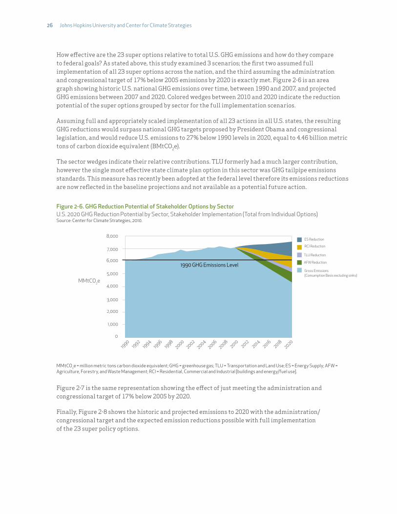
How e!ective are the 23 super options relative to total U.S. GHG emissions and how do they compare to federal goals? As stated above, this study examined 3 scenarios; the first two assumed full implementation of all 23 super options across the nation, and the third assuming the administration and congressional target of 17% below 2005 emissions by 2020 is exactly met. Figure 2-6 is an area graph showing historic U.S. national GHG emissions over time, between 1990 and 2007, and projected GHG emissions between 2007 and 2020. Colored wedges between 2010 and 2020 indicate the reduction potential of the super options grouped by sector for the full implementation scenarios.
Assuming full and appropriately scaled implementation of all 23 actions in all U.S. states, the resulting GHG reductions would surpass national GHG targets proposed by President Obama and congressional legislation, and would reduce U.S. emissions to 27% below 1990 levels in 2020, equal to 4.46 billion metric tons of carbon dioxide equivalent (BMtCO2e).
The sector wedges indicate their relative contributions. TLU formerly had a much larger contribution, however the single most e!ective state climate plan option in this sector was GHG tailpipe emissions standards. This measure has recently been adopted at the federal level therefore its emissions reductions are now reflected in the baseline projections and not available as a potential future action.
Figure 2-6. GHG Reduction Potential of Stakeholder Options by Sector U.S. 2020 GHG Reduction Potential by Sector, Stakeholder Implementation (Total from Individual Options)Source: Center for Climate Strategies, 2010.
MMtCO2e
0
19901992
19941996
19982000
20022004
20062008
20102012
20142016
20182020
1,000
2,000
3,000
4,000
5,000
6,000
7,000
8,000
1990 GHG Emissions Level
ES Reduction
RCI Reduction
TLU Reduction
AFW Reduction
Gross Emissions(Consumption Basis excluding sinks)
MMtCO2e = million metric tons carbon dioxide equivalent; GHG = greenhouse gas; TLU = Transportation and Land Use; ES = Energy Supply; AFW = Agriculture, Forestry, and Waste Management; RCI"="Residential, Commercial and Industrial [buildings and energy/fuel use].
Figure 2-7 is the same representation showing the e!ect of just meeting the administration and congressional target of 17% below 2005 by 2020.
Finally, Figure 2-8 shows the historic and projected emissions to 2020 with the administration/congressional target and the expected emission reductions possible with full implementation of the 23 super policy options.

Impacts of Comprehensive Climate and Energy Policy Options on the U.S. Economy !27
Figure 2-7. Stakeholder Policies Scaled to Achieve Congressional GHG Target U.S. 2020 GHG Reduction Potential by Sector, Congressional Implementation (Total from Individual Options)Source: Center for Climate Strategies, 2010.
MMtCO2e
0
19901992
19941996
19982000
20022004
20062008
20102012
20142016
20182020
1,000
2,000
3,000
4,000
5,000
6,000
7,000
8,000
1990 GHG Emissions Level
ES Reduction
RCI Reduction
TLU Reduction
AFW Reduction
Gross Emissions(Consumption Basis excluding sinks)
MMtCO2e = million metric tons carbon dioxide equivalent; GHG = greenhouse gas; TLU = Transportation and Land Use; ES = Energy Supply; AFW = Agriculture, Forestry, and Waste Management; RCI"="Residential, Commercial, and Industrial [buildings and energy/fuel use].
Figure 2-8. GHG Reductions – Stakeholder and Congressional Target Scenarios U.S. 1990-2020 GHG Reduction Potential, Congressional Target and Stakeholder Target ScenariosSource: Center for Climate Strategies, 2010.
GHG = greenhouse gas; MMtCO2e = million metric tons carbon dioxide equivalent.
MMtCO2e
0
19901992
19941996
19982000
20022004
20062008
20102012
20142016
20182020
1,000
2,000
3,000
4,000
5,000
6,000
7,000
8,000
9,000Baseline Emissions Stakeholder TargetCongressional Target

28!Johns Hopkins University and Center for Climate Strategies
I. IntroductionSince 2000, 34 U.S. states have completed or are developing Greenhouse Gas (GHG) reduction plans that evaluate and recommend specific policy options to achieve climate change stabilization targets and other important policy objectives including economic, energy and environmental security. The major focus has typically been on the direct, or on-site, impacts (such as cost-e!ectiveness or microeconomic analysis) of individual mitigation options and aggregate portfolios of actions (see section 2). However, the political needs of implementation also typically require assessment of indirect e!ects, including macroeconomic impacts, and in some cases detailed distributional impacts.
The importance of indirect and distributional impacts are clear to policy makers. For instance, some policy options can result in cost-savings directly to those who implement them as well as gains to their customers if the savings are passed on in the form of lower prices. However, these gains may come at the cost of others who provide investment outlays or su!er reduced sales of energy. Some policy options will incur additional costs to businesses, households, nonprofit institutions, and government operations, and the likely cutback in economic activity will also a!ect their suppliers. The 23 climate mitigation policy option results presented in Section 2 reflect the net direct costs or savings associated with their implementation, but they do not include the ripple e!ects of decreased or increased spending on mitigation, and the interaction of demand and supply in various markets. For example, reduction in consumer demand for electricity reduces the demand for generation by all sources, including both fossil energy and renewables. It therefore reduces the demand for fuel inputs such as coal and natural gas. Moreover, the investment in new equipment may partially or totally o!set expenditures on ordinary plant operations and equipment. At the same time, businesses and households whose electricity bills have decreased have more money to spend on other goods and services. If the households purchase more food or clothing, this stimulates the production of these goods, at least in part, within the state. Food processing and clothing manufacturers in turn purchase more raw materials and hire more employees. Then raw material suppliers in turn purchase more of the inputs they need, and the additional employees of all these firms in the supply chain purchase more goods and services from their wages and salaries. The sum total of these “indirect” impacts is some multiple of the original direct on site impact; hence this is o#en referred to as the multiplier e!ect, a key aspect of macroeconomic impacts. It applies to both increases and decreases in economic activity. It can be further stimulated by price decreases and muted by price increases.
The extent of the many types of linkages in the economy and macroeconomic impacts is extensive and cannot be traced by a simple set of calculations. It requires the use of a sophisticated model that reflects the major structural features of an economy, the workings of its markets, and all of the interactions between them. In this study, we used the Regional Economic Models, Inc. (REMI) Policy Insight Plus (PI+) modeling so#ware to be discussed below (REMI, 2009) to evaluate the macroeconomic impacts to the U.S. of implementing the 23 GHG mitigation super options across the states. The REMI model is the most widely used economic modeling so#ware package in the U.S. and has been heavily peer reviewed. The model is used extensively to measure proposed legislative and other program and policy economic impacts across the private and public sectors by government agencies in nearly every state of the U.S. In addition, it is o#en the tool of choice to measure these impacts by a number of university researchers and private research groups that evaluate economic impacts across a state and nation.
%&'()*+ (./&&
» Macroeconomic E#ects of Mitigation Options: REMI Model Analysis
Impacts of Comprehensive Climate and Energy Policy Options on the U.S. Economy !29
In order to perform macroeconomic impact analysis of climate action plans using REMI, information is needed on basic microeconomic considerations, such as the direct costs and direct savings of each GHG mitigation option, as well as on aspects that relate to macro linkages. The results reported in the state action plans include GHG reduction potentials, net cost/savings in Net Present Value (NPV), and cost-e!ectiveness (per ton cost/saving of GHG removed). The macro study needs more detailed and disaggregated information on both the costs and savings aspects. For example, program costs need to be disaggregated into capital cost, operation and maintenance (O&M) cost, and fuel cost; energy savings need to be specified in di!erent types of energy and for specific economic sectors. In addition, all these data are needed for individual years in the study period (2010-2020).
This level of detailed information may not always be reported in the state action plans for each option. Therefore, it was necessary to obtain the calculation workbooks used to quantify the policy options, and to extract the data needed by the REMI analysis from the workbooks. Because of the time limitation of this study, our study focused our data collection for macroeconomic linkage variables on seven states (Colorado, Florida, Iowa, Michigan, North Carolina, Pennsylvania, and Washington) that we believe are representatives of national diversity, and used the weighted average costs and savings of each individual super option to get the scaled-up estimates at the national level. Please refer to the separate document Annex D* for a summary of the methodology used in the scale-up estimation.
This report is structured as follows: Subsection II describes the 3 modeling scenarios analyzed, Subsection III is an overview of the REMI model (see greater detail in Annex C*), Subsection IV reviews how the data from the climate plan was used in the REMI analysis, Subsection V reviews the setup of the REMI simulation, Subsection VI presents the REMI results for Scenario 1, Subsection VII summarizes the major features of the Kerry-Lieberman Senate bill, and Subsection VIII presents the analyses of two hybrid scenarios of the Kerry-Lieberman bill and the Stakeholder recommended policies and measures.
II. Three Modeling ScenariosThe purpose of this section is to estimate the macroeconomic impacts of three scenarios representing di!erent applications of stakeholder recommended policies and measures, including recent climate change legislation in the form of the U.S. Senate bill sponsored by Senators Kerry and Lieberman. The impacts are expressed in terms of major macroeconomic indicators – output, employment, and income— for the economy as a whole and for each of 169 sectors of the economy, for all years in the study period under Scenario 1 (2010-2020) and the year 2020 under Scenarios 2 and 3.
For Scenarios 2 and 3 we identify the major features of the Senate bill relating to the emission cap, sectors covered by cap and trade and other major policy instruments, the allocation of allowances, and the potential to use o!sets from domestic and international sources, and the government spending (“recycling”) of allowance auction revenue.
Scenario 1. Stakeholder ScenarioThis case assumes the full implementation of all 23 mitigation options described and presented in Section 2. It assumes that all measures described in Annex B* are implemented in all 50 states using the national scale-up methodology described in Annex A.*
Scenario 2. Stakeholder/Senate Scenario This case assumes full implementation of the 23 measures in all 50 states, but it also includes the application of a limited federal cap-and-trade program as contemplated in the Kerry-Lieberman (K-L) bill and described in detail in Annex F.*
* The Annexes to this report are available at energypolicyreport.jhu.edu.

30!Johns Hopkins University and Center for Climate Strategies
Scenario 3. Senate ScenarioIn this simulation case we model the major features of the K-L bill, including cap-and-trade, using the 23 super option measures as in Scenario 2, except in this case we limit the GHG reduction benefits to precisely match the national reduction goal stated in the legislation.
III. REMI Model AnalysisSeveral modeling approaches can be used to estimate the total regional economic impacts of environmental policy, including both direct (on-site) e!ects and various types of indirect (o!-site) e!ects. These include: input-output (I-O), computable generated equilibrium (CGE), mathematical programming (MP), and macroeconometric (ME) models. Each has its own strengths and weaknesses (see, e.g., Rose and Miernyk, 1989; Partridge and Rickman, 1998).1
The choice of which model to use depends on the purpose of the analysis and various considerations that can be considered as performance criteria, such as accuracy, transparency, manageability, and costs. A#er careful consideration of these criteria, we chose to use the REMI PI+ model. The REMI model is superior to the other reviewed in terms of its forecasting ability1 and is comparable to CGE models in terms of analytical power and accuracy. With careful explanation of the model, its application, and its results, it can be made as transparent as any of the others.
The REMI model has evolved over the course of 30 years of refinement (see, e.g., Treyz, 1993). It is a packaged so#ware program, but is built with a combination of national and region-specific data. Government agencies in practically every state in the U.S. have used a REMI model for a variety of purposes, including evaluating the impacts of the change in tax rates, the exit or entry of major businesses in particular or economic programs in general, and, more recently, the impacts of energy and/or environmental policy actions.
A detailed discussion of the major features of the REMI PI+ model is presented in Annex C.* We simply provide a summary for general readers here. A macroeconometric forecasting model covers the entire economy, typically in a “top-down” manner, based on macroeconomic aggregate relationships, such as consumption and investment. REMI di!ers somewhat in that it includes some key relationships, such as exports, in a bo"om-up approach. In fact, it makes use of the finely grained sectoring detail of an I-O model, i.e., in the version we used it divides the economy into 169 sectors, thereby allowing important di!erentials between them. This is especially important in a context of analyzing the impacts of GHG mitigation actions, where various options were fine-tuned to a given sector or where they directly a!ect several sectors somewhat di!erently.
The macroeconomic character of the model is able to analyze the interactions between sectors (ordinary multiplier e!ects) but with some refinement for price changes not found in I-O models. The REMI PI+ model also brings into play features of labor and capital markets, as well as trade with other states or countries, including changes in competitiveness.
The econometric feature of the model refers to two considerations. The first is that the model is based on inferential statistical estimation of key parameters based on pooled time series and regional (panel) data across all states of the U.S. (the other candidate models use “calibration,” based on a single year’s data).2 This gives the REMI PI+ model an additional capability of being be"er able to extrapolate3 the future course of the economy, a capability the other models lack. The major limitation of the REMI PI+ model versus the others is that it is pre-packaged and not readily adjustable to any unique features of the case in point. The other models, because they are based on less data and a less formal estimation procedure,
1. Statistically estimated time series models are best suited to forecasting, but were not among the candidates considered here because our emphasis was on policy analysis.2. REMI is the only one of the models reviewed that really addresses the fact that many impacts take time to materialize and that the size of impacts changes over time as prices and wages adjust. In short, it be$er incorporates the actual dynamics of the economy. 3. The model can be used alone for forecasting with some caveats, or used in conjunction with other forecast “drivers.“
Impacts of Comprehensive Climate and Energy Policy Options on the U.S. Economy !31
can more readily accommodate data changes in technology that might be inferred, for example from engineering data. However, our assessment of the REMI PI+ model is that these adjustments were not needed for the purpose at hand.
The use of the REMI PI+ model involves the generation of a baseline forecast of the economy through 2020. Then simulations are run of the changes brought about through the implementation of the various GHG mitigation options. Again, this includes the direct e!ects in the sectors in which the options are implemented, and then the combination of multiplier (purely quantitative interactions) general equilibrium (price-quantity interactions) and macroeconomic (aggregate interactions) impacts. The di!erences between the baseline and the “counter-factual” simulation represent the total regional economic impacts of these policy options.
IV. Input Data 1. REMI PI+ Model Input Development The quantification analysis of the costs/savings undertaken by the state stakeholder processes and the updates performed for this study by the sectoral analysts were limited to the direct e!ects of implementing the options. For example, the direct costs of an energy e$ciency option include the ratepayers’ payment for the program and the energy customers’ expenditure on energy e$ciency equipments and devices. The direct benefits of this option include the savings on energy bills of the customers.
As described in Section 2, these state level microeconomic analyses have been scaled up to the national level. To supplement the microeconomic analysis the REMI PI+ model was selected to evaluate macroeconomic impacts (such as gross domestic output, employment, and personal income) of every major option (the super options) that had been identified by various states. The U.S. two-region REMI PI+ model used in this study is based on panel data through 2007.4 In addition, we chose the larger 169-sector U.S. REMI model over the 70-sector model to undertake the macroeconomic analysis. The standard 70-sector REMI model is not as adequate as the 169-sector model to evaluate the impacts of the various GHG mitigation policy options because the former combines electricity, gas and water into a single Utilities sector, while the la"er separates the three activities into individual sectors.
Before undertaking any economic simulations, the costs and savings for each policy option are translated to model inputs that can be utilized in the model. This step involves the selection of appropriate policy levers in the REMI PI+ model to simulate the policy’s changes. The input data include sectoral spending and savings over the full time horizon (2010-2020) of the analysis. In Tables 2-5, we choose one example option from each of the Residential, Commercial and Industrial (RCI), Energy Supply (ES), Agriculture, Forestry and Waste Management (AFW), and Transportation and Land Use (TLU) sectors to illustrate how we translate, or map, the TWG results into REMI PI+ economic variable inputs.
Using RCI-1 Demand Side Management (DSM) as an example, the first set of inputs in Table 3-1 is the increased cost to the Commercial, Industrial, and Residential sectors due to the purchases of energy e$cient equipment and appliances. For the Commercial and Industrial sectors, this is simulated in REMI by increasing the value of the “Capital Cost” variable of individual Commercial sectors and individual Industrial sectors under the “Compensation, Prices, and Costs Block.” For the Residential sector, the program costs (which represent total incremental costs of new equipment over conventional equipment) are simulated by increasing the “Consumer Spending” on “Kitchen & Other Household Appliances” (and decreasing all the other consumptions correspondingly). The “Consumer Spending (amount)” and “Consumption Reallocation (amount)” variables can be found in the “Output and Demand Block” in the REMI model.
4. The REMI model construction methodology is typically applied at the regional level, with at least a two-region set-up (the target region and the rest of the U.S.). Even the national model must be constructed in this manner. In this study, the two regions are Esmeralda County, NV and the rest of U.S. Given the low population (less than 700) and small economy size (less than 14 million GDP) of Esmeralda County, there is negligible inaccuracy in treating the second region (the rest of U.S.) as the entire country. One di#erence in this “single entity” approximation is that there is no interregional migration e#ect.

32!Johns Hopkins University and Center for Climate Strategies
The second set of inputs are the corresponding stimulus e!ect to the economy of the spending on e$cient equipment and appliances, i.e., the increase in the final demand for goods and services from the industries that supply energy e$cient equipment and appliances. This is simulated in REMI by increasing the “Exogenous Final Demand” (in the “Output and Demand Block”) of the following sectors: Ventilation, Heating, Air-conditioning, and Commercial Refrigeration Equipment Manufacturing sector; Electric Lighting Equipment Manufacturing sector; Electrical Equipment Manufacturing sector; and Other Electrical Equipment and Component Manufacturing sector. The interest payment due to the financing of the capital investment is simulated as the “Exogenous Final Demand” increase of the Monetary Authorities, Credit Intermediation sector.5 The administrative cost of the DSM program is simulated as the “Exogenous Final Demand” increase of the Management, Scientific, and Technical Consulting Services sector.
Table 3-1. Mapping the Direct Economic Impacts of RCI-1 Demand Side Management into REMI VariablesDirect Economic Impacts Policy Variable Selection in REMI
Customer Outlay on Energy E$ciency (EE)
Businesses (Commercial and Industrial Sectors)
Compensation, Prices, and Costs Block 0Capital Cost (amount) of individual commercial sectors 0 Increase
Households (Residential Sector)
Output and Demand Block 0 Consumer Spending (amount) 0 Kitchen & other household appliancesa 0 Increase
Output and Demand Block 0 Consumer Spending (amount) 0 Bank Service Charges 0 Increase
Output and Demand Block 0Consumption Reallocation (amount) 0 All Consumption Sectors 0Decrease
Investment in EE Technologies
Output and Demand Block 0 Exogenous Final Demand (amount) for Ventilation, Heating, Air-conditioning, and Commercial Refrigeration Equipment Manufacturing sector; Electric Lighting Equipment Manufacturing sector; Electrical Equipment Manufacturing sector; and Other Electrical Equipment and Component Manufacturing sector 0 Increase
Interest Payment of Financing Capital Investment
Output and Demand Block 0 Exogenous Final Demand (amount) for Monetary Authorities, Credit Intermediation sector0Increase
Administrative OutlaysOutput and Demand Block 0 Exogenous Final Demand (amount) for Management, Scientific, and Technical Consulting Services sector 0 Increase
Energy Savings of the Customers
Businesses (Commercial and Industrial Sectors)
Compensation, Prices, and Costs Block 0 Electricity, Natural Gas, and Residual (Commercial Sectors) Fuel Cost (share) of All Commercial Sectors 0 Decrease
Compensation, Prices, and Costs Block0 Electricity, Natural Gas, and Residual (Industrial Sectors) Fuel Cost (share) of All Industrial Sectors0 Decrease
Households (Residential Sector)
Output and Demand Block 0 Consumer Spending (amount) 0 Electricity, Gas, and Fuel Oil 0 Decrease
Output and Demand Block 0 Consumption Reallocation (amount) 0 All Consumption Sectors 0 Increase
Energy Demand Decrease from the Energy Supply Sectorsb
Output and Demand Block 0 Exogenous Final Demand (amount) for Electric Power Generation, Transmission, and Distribution sector; Natural Gas Distribution sector; and Petroleum and Coal Products Manufacturing sector 0 Decrease
a. Since there is no specific consumer expenditure category for furnaces, it is included in the investment in EE technologies in the row below. Home insulation and sealing services and other associated measures are included in the simulations of RCI-2 High Performance Buildings and RCI-4 Building Codes policy options. b. The final demand change here only reflects the energy consumption reductions from the Commercial and Industrial sectors; Residential sector reductions are entered in the model’s “Consumer Spending” variable.
5. The opportunity cost of the interest payment is included in the increase of the “Capital Cost” variable for the Commercial and Industrial sectors (row 1 in Table 3-1). As for the Residential sector, it is reflected in the reduction in consumption of all other commodities (i.e., this is reflected in a decrease in the “Consumption Reallocation” variable shown in row 2 in Table 3-1).

Impacts of Comprehensive Climate and Energy Policy Options on the U.S. Economy !33
Table 3-2. Mapping the Direct Economic Impacts of ES-1 Renewable Portfolio Standard into REMI Variables
Direct Economic Impacts Policy Variable Selection in REMI
Incremental Capital Cost of Electricity Generation (Renewable minus Avoided Traditional)
Compensation, Prices, and Costs Block 0 Capital Cost (amount) of Electric Power Generation, Transmission, and Distribution sectors0Increase
Incremental O&M Cost of Electricity Generation (Renewable minus Avoided Traditional)
Compensation, Prices, and Costs Block 0 Production Cost (amount) of Electric Power Generation, Transmission, and Distribution sectors0Increase
Reduction on Fuel Cost of Electricity Generation
Compensation, Prices, and Costs Block 0 Production Cost (amount) of Electric Power Generation, Transmission, and Distribution sectors0Decrease
Incremental Investment in Generation Technologies (Renewable minus Avoided Traditional)
Output and Demand Block 0 Exogenous Final Demand (amount) for Construction sector 0 Increase
Output and Demand Block 0 Exogenous Final Demand (amount) for Engine, Turbine, and Power Transmission Equipment Manufacturing sector 0 Increase
Interest Payment of Financing Capital Investment
Output and Demand Block 0 Exogenous Final Demand (amount) for Monetary Authorities, Credit Intermediation sector 0 Increase
Renewable (Biomass) Fuel InputsOutput and Demand Block 0 Exogenous Final Demand (amount) for Waste Collection; Waste Treatment and Disposal and Waste Management Services sector and Forestry sector 0 Increase
Fossil Fuel Savings Output and Demand Block 0 Exogenous Final Demand (amount) for Coal Mining sector, Oil and Gas Extraction sector, and Pipeline Transportation sector 0 Decreasea
Tax Credits to Renewable Electricity Generation Output and Demand Block 0 State Government spending (amount) 0 Decrease
a Assume the displaced electricity generations are 50% coal-fired electricity and 50% NG-fired electricity.
Table 3-3. Mapping the Direct Economic Impacts of AFW-5 Urban Forestry into REMI Variables
Direct Economic Impacts Policy Variable Selection in REMI
Spending StimulationOutput and Demand Block 0 Exogenous Final Demand (amount) for Forestry; Fishing, Hunting and Trapping sector and Support Activities for Agriculture and Forestry sector 0 Increase
Cost of Urban Forestry Output and Demand Block 0 Local Government spending (amount) 0 Decreasea
Energy Savings (reduction in electricity consumption)
Commercial Sectors Compensation, Prices, and Costs Block 0 Electricity (Commercial Sectors) Fuel Cost (amount) of All Commercial Sectors 0 Decreaseb
Households (Residential Sector)
Output and Demand Block 0 Consumer Spending (amount) 0 Electricity 0 Decreaseb
Output and Demand Block 0 Consumption Reallocation (amount) 0All Consumption Categories 0 Increase
Government Output and Demand Block 0 Local Government spending (amount) 0 Decreaseb
Electricity Demand Decrease from the Utility Sectorc
Output and Demand Block 0 Exogenous Final Demand (amount) for Electric Power Generation, Transmission, and Distribution sector 0 Decrease
a It is assumed that all the costs of urban forestry program will be borne by the local government. Accordingly, we assume the local government spend-ing elsewhere will be reduced by the same amount of spending on the urban forestry program. b It is assumed that energy savings resulted from shading of structures will be split between the Commercial sector, Residential sector, and Government by 40%, 40%, and 20%.c The final demand change here only reflects the energy consumption reductions from the Commercial and Industrial sectors. The Residential sector energy consumption reductions will be entered into the model through the “Consumer Spending” variable.

34!Johns Hopkins University and Center for Climate Strategies
Table 3-4. Mapping the Direct Economic Impacts of TLU-6 Mode Shi% from Truck to Rail into REMI Variables
Direct Economic Impacts Policy Variable Selection in REMI
Cost of Additional Terminal and Track Upgrades
Compensation, Prices, and Costs Block 0 Capital Cost of Rail Transportation sector 0 Increase
Investment to Improve Rail Transportation System
Output and Demand Block 0Exogenous Final Demand (amount) for Construction sector 0 Increase
Interest Payment of Financing Capital Investment
Output and Demand Block 0 Exogenous Final Demand (amount) for Monetary Authorities, Credit Intermediation sector 0 Increase
Fuel Savings
Compensation, Prices, and Costs Block 0 Residual Fuel Costa for Truck Transportation sector 0 Decrease
Compensation, Prices, and Costs Block 0 Residual Fuel Cost (amount) of All Commercial and Industrial sectors 0Decrease
Fuel Demand Decrease of Fuel Output and Demand Block 0 Exogenous Final Demand (amount) for Petroleum and Coal Products Manufacturing sector 0Decrease
a In the REMI model, residual fuel includes all energy fuels other than electricity and natural gas.
The third set of inputs to REMI presents the energy savings of the Commercial, Industrial, and Residential sectors resulting from the DSM program. For the Commercial and Industrial sectors, the energy savings are simulated in REMI by decreasing the value of the “Electricity/Natural Gas/Residual Fuel Cost of All Commercial/Industrial Sectors” variables. These variables can be found in the “Compensation, Prices, and Costs Block.” For the Residential sector, the energy savings are simulated by decreasing the “Consumer Spending” on “Electricity,” “Gas” and “Fuel Oil” (and increasing all the other consumption categories correspondingly). Again, the “Consumer Spending (amount)” and “Consumption Reallocation (amount)” variables can be found in the “Output and Demand Block” in the REMI model.
The last set of inputs are the corresponding damping e!ects to the Energy Supply sector due to the decrease in the demand from the customer sectors. These e!ects are simulated by reducing the “Exogenous Final Demand” of the Electric Power Generation, Transmission, and Distribution sector, Natural Gas Distribution sector, and Petroleum and Coal Products Manufacturing sector in REMI.6 In this step, the final demand change is only modeled for the non-residential sectors, i.e., only the decreased demand from the Commercial and Industrial sectors need to be manually entered into the model as final demand change for the energy supply sectors. For the Residential sector, the model will internally convert the change in the Consumer Spending (amount) policy variable into changes in final demand for the corresponding sectors.
2. Modeling AssumptionsThe major data sources of the analysis are the scaled-up quantification results on costs and savings of various mitigation policy options. However, we supplement these with some additional data and assumptions in the REMI analysis in cases where these costs and some conditions relating to the implementation of the options are not specified in the micro analysis or are not known with certainty. Below is the list of major assumptions we adopted in the analysis:
1.-In the base case analysis, for all the policy options that involve capital investment, we simulated a stimulus from only 50% of the capital investment requirements. This is based on the assumption that 50% of the incremental investment in new equipment will simply displace other investment in the state.
6. The values of energy demand reductions are scaled up from the state level estimates of energy consumption changes in di#erent customer sectors due to the implementation of various mitigation options. They are not derived from the REMI model runs, instead they are exogenously computed and fed into the REMI model as simulation inputs.
Impacts of Comprehensive Climate and Energy Policy Options on the U.S. Economy !35
2.-Capital investment in power generation is split 60:40 between sectors that provide generating equipment and the Construction sector for large power plants (such as coal-fired power plants), and 80:20 for smaller installations (mainly renewables).
3.-For the RCI options, the energy consumers’ participant costs of energy e$ciency programs are computed for the Residential, Commercial, and/or Industrial sectors by the state level technical working groups (TWGs). For the Commercial and Industrial sectors, the TWGs’ analyses only provide the aggregated costs for the entire Commercial sector and the entire Industrial sector. Since in the REMI model capital cost and production cost variables can only be simulated for individual Commercial sectors or Industrial sectors, we distributed these costs among the 169 REMI sectors based on the national input-output data provided in the REMI model in relation to the delivery of utility services to individual sectors.
4.-The interest payment and the administrative cost are split out from the levelized cost using the following assumptions: a. For the RCI options, it is assumed that 50% of the RCI costs will be covered by private-sector financing and 50% will be covered by the utility expenditures, such as those supported by public benefit charges. The administrative costs are assumed to account for 10% of the 50% utility portion of the capital costs. b. For the ES, AFW, and TLU options that involve capital investment, we assume 100% of the total costs will be covered by financing.
5.-For the Combined Heat and Power option, the total costs of installing the CHP systems are only available for the Commercial and Industrial sectors as a whole from the micro analysis. We used the energy consumption data by sector as the basis to distribute the costs among the REMI sectors.
6.-For the Restoration/A!orestation option, it is assumed that the costs are borne by the private sector (farmers). The potential future cost savings from forest products (e.g., merchantable timber or bioenergy feedstocks) are not taken into account, since these cost savings would most likely not be realized during the period of this analysis.
7.-For the Urban Forestry option, it is assumed that all the costs will be borne by the local government. It is also assumed that increasing the government spending in the urban forestry program will be o!set by a decrease in the same amount of government spending on other goods and services. The energy savings breakout is 20% Government, 40% Commercial sector, and 40% Residential sector.
8.-For the TLU options related to fuel cost changes for heavy duty trucks, we distribute 45% of the fuel savings (or cost increase) to the Truck Transportation sector based on the Vehicle Inventory and Use Survey data that about 45% of the miles accumulated by heavy trucks are for the “For-Hire” transportation and 55% are for the “Own Account Transportation” (U.S. Census Bureau, 2002). Further, the 55% of the fuel savings (or cost increase) are distributed across sectors other than the Truck Transportation sector in the economy in proportion to the petroleum inputs for each sector.
9.-For the RPS option and the nuclear power option, we assume that the displaced electricity generation from fossil fuels is split half and half between coal-fired electricity and gas-fired electricity. This assumption is based on the fact that in Iowa and Pennsylvania, all displaced electricity is assumed to be coal, in Florida and Arkansas, it is assumed to be all gas, while in other CCS-facilitated states, the displacement is a mix of the two.

36!Johns Hopkins University and Center for Climate Strategies
V. Simulation Set-up in REMIFigure 3-1 shows how a policy simulation process is undertaken in the REMI PI+ model. First, a policy question is formulated (such as what would be the economic impacts of implementing the Demand Side Management Programs). Second, external policy variables that would embody the e!ects of the policy are identified (take DSM as an example, relevant policy variables would include incremental costs and investment in energy e$cient appliances; final demand increase in the sectors that produce the equipments and appliances; and the avoided consumption of electricity, natural gas, etc.). Third, baseline values for all the policy variables are used to generate the control forecast (baseline forecast). In REMI PI+, the baseline forecast uses the most recent data available (i.e., 2007 data) for the study region and the external policy variables are set equal to their baseline values. Fourth, an alternative forecast is generated by changing the values of the external policy variables. Usually, the changing values of these variables represent the direct e!ects of the simulated policy scenario. For example, in our analysis of the DSM option, the costs to the Commercial and Residential sectors and the avoided consumption of energy were based on the scale-up of the technical assessment of implementing this mitigation option in the CCS facilitated states. Fi#h, the e!ects of the policy scenario are measured by comparing the baseline forecast and the alternative forecast. Sensitivity analysis can be undertaken by running a series of alternative forecasts with di!erent assumptions on the values of the policy variables.
In this study, we first ran the REMI PI+ model for each of the 23 super options individually in a comparative static manner, i.e., one at a time, holding everything else constant. Next, we ran a simultaneous simulation in which we assume that all the super options are implemented together.
Figure 3-1. Process of Policy Simulation in REMI
What e!ect wouldPolicy X have?
Changes in policy variablesassociated with
Policy X
Baseline values for all
policy variables
Control ForecastAlternative Forecast
The REMI Model
Compare Forecasts
REMI = Regional Economic Models, Inc.
Then the simple summation of the e!ects of individual options was compared to the simultaneous simulation results to determine whether the “whole” is di!erent from the “sum” of the parts. Di!erences can arise from non-linearities and/or synergies. The la"er would stem from complex functional relationships in the REMI PI+ model.
Before performing the simulations in REMI PI+, overlaps between options within the same sector and across di!erent sectors were eliminated.

Impacts of Comprehensive Climate and Energy Policy Options on the U.S. Economy !37
VI. Presentation of the Results – Scenario 1- Stakeholder Recommendations 1. Basic ResultsThe results of the macroeconomic simulation of Scenario 1, the stakeholder recommendations without cap-and-trade or other features of proposed legislation are presented here. Following a discussion of the Kerry-Lieberman bill in Subsection VII, the results of the 2 scenarios involving provisions of the K-L bill are presented in Subsection VIII.
A summary of the basic results of the application of the REMI PI+ model to determine the macroeconomic impacts of the individual mitigation super options analyzed in this study is presented in Tables 3-5 and 3-6. Table 3-5 includes the GDP impacts for each super option for three selected years, as well as a net present value (NPV) calculation for the entire period of 2010 to 2020. Table 3-6 presents analogous results for employment impacts, though, for reasons noted below, an NPV calculation of employment impacts is not appropriate.
Table 3-5. Gross Domestic Product Impacts of the 23 GHG Mitigation Policy Options (billions of fixed 2007 dollars)
Policy Options 2010 2012 2015 2020 NPV
ES-1 Renewable Portfolio Standard –$0.25 –$2.27 –$5.32 –$5.35 –$35.52
ES-2 Nuclear $0.00 –$0.07 –$0.46 –$6.85 –$8.14
ES-3 Carbon Capture and Storage or Reuse (CCSR) $0.00 $0.00 –$2.80 –$4.47 –$16.57
ES-4 Coal Plant E$ciency Improvements $0.01 $0.02 $0.04 $0.48 $0.86
Subtotal – Energy Supply (ES) –$0.24 –$2.32 –$8.57 –$16.19 –$59.38
RCI-1 Demand Side Management Programs $4.82 $16.17 $36.19 $90.05 $305.05
RCI-2 High Performance Buildings $0.84 $1.73 $4.72 $12.12 $40.14
RCI-3 Appliance standards $0.02 –$0.04 –$0.12 $0.05 –$0.43
RCI-4 Building Codes $0.89 $2.68 $6.06 $13.65 $49.05
RCI-5 Combined Heat and Power –$3.79 –$8.57 –$14.08 –$21.17 –$104.38
Subtotal – Residential Commercial and Industrial (RCI) $2.79 $11.99 $32.77 $94.68 $289.44
AFW-1 Crop Production Practices $0.08 $1.05 $2.28 $4.55 $17.50
AFW-2 Livestock Manure –$0.01 –$0.02 –$0.07 –$0.17 –$0.58
AFW-3 Forest Retention $0.06 $0.31 $0.57 $0.48 $3.45
AFW-4 Reforestation/A!orestation –$5.92 –$7.67 –$9.23 –$11.07 –$73.47
AFW-5 Urban Forestry $1.32 $4.75 $5.95 $5.44 $40.12
AFW-6 Source Reduction $0.04 $0.62 $1.45 $2.53 $10.37
AFW-7 Enhanced Recycling of MSW $0.88 $3.49 $7.94 $10.38 $51.61
AFW-8 MSW Landfill Gas Management $1.02 $1.57 $2.61 $10.44 $26.47
Subtotal – Agriculture, Forestry & Waste (AFW) –$2.52 $4.09 $11.51 $22.58 $75.46
TLU-1 Vehicle Purchase Incentives $0.02 $0.62 $3.78 $16.51 $39.64
TLU-2 Renewable Fuel Standard –$0.02 –$0.27 –$2.38 –$4.78 –$17.08
TLU-3 Smart Growth $0.18 $0.89 $2.32 $6.15 $19.54
TLU-4 Transit –$0.05 $0.00 $0.23 $1.18 $2.46
TLU-5 Anti-Idling Technologies and Practices –$0.08 $0.01 $0.18 $1.92 $2.96
TLU-6 Mode Shi# from Truck to Rail –$0.44 –$2.39 –$0.56 $6.69 $2.92
Subtotal – Transportation and Land Use (TLU) –$0.38 –$1.15 $3.56 $27.68 $50.45
Summation Total –$0.34 $12.60 $39.28 $128.76 $355.97
Simultaneous Total –$0.34 $12.68 $41.34 $159.60 $406.74
GHG = greenhouse gas; MSW = municipal solid waste; NPV = net present value. Note: A positive number in this table means a positive stimulus to the economy, or an increase in the gross domestic product (GDP); a negative number in this table means a negative impact to the economy, or a decrease in the GDP.
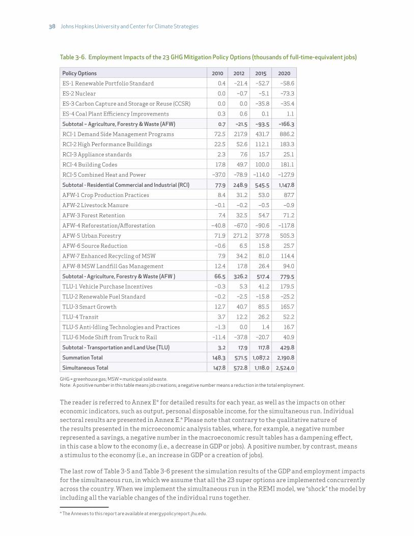
38!Johns Hopkins University and Center for Climate Strategies
Table 3-6. Employment Impacts of the 23 GHG Mitigation Policy Options (thousands of full-time-equivalent jobs)
Policy Options 2010 2012 2015 2020
ES-1 Renewable Portfolio Standard 0.4 –21.4 –52.7 –58.6
ES-2 Nuclear 0.0 –0.7 –5.1 –73.3
ES-3 Carbon Capture and Storage or Reuse (CCSR) 0.0 0.0 –35.8 –35.4
ES-4 Coal Plant E$ciency Improvements 0.3 0.6 0.1 1.1
Subtotal – Agriculture, Forestry & Waste (AFW) 0.7 –21.5 –93.5 –166.3
RCI-1 Demand Side Management Programs 72.5 217.9 431.7 886.2
RCI-2 High Performance Buildings 22.5 52.6 112.1 183.3
RCI-3 Appliance standards 2.3 7.6 15.7 25.1
RCI-4 Building Codes 17.8 49.7 100.0 181.1
RCI-5 Combined Heat and Power –37.0 –78.9 –114.0 –127.9
Subtotal - Residential Commercial and Industrial (RCI) 77.9 248.9 545.5 1,147.8
AFW-1 Crop Production Practices 8.4 31.2 53.0 87.7
AFW-2 Livestock Manure –0.1 –0.2 –0.5 –0.9
AFW-3 Forest Retention 7.4 32.5 54.7 71.2
AFW-4 Reforestation/A!orestation –40.8 –67.0 –90.6 –117.8
AFW-5 Urban Forestry 71.9 271.2 377.8 505.3
AFW-6 Source Reduction –0.6 6.5 15.8 25.7
AFW-7 Enhanced Recycling of MSW 7.9 34.2 81.0 114.4
AFW-8 MSW Landfill Gas Management 12.4 17.8 26.4 94.0
Subtotal - Agriculture, Forestry & Waste (AFW#) 66.5 326.2 517.4 779.5
TLU-1 Vehicle Purchase Incentives –0.3 5.3 41.2 179.5
TLU-2 Renewable Fuel Standard –0.2 –2.5 –15.8 –25.2
TLU-3 Smart Growth 12.7 40.7 85.5 165.7
TLU-4 Transit 3.7 12.2 26.2 52.2
TLU-5 Anti-Idling Technologies and Practices –1.3 0.0 1.4 16.7
TLU-6 Mode Shi# from Truck to Rail –11.4 –37.8 –20.7 40.9
Subtotal - Transportation and Land Use (TLU) 3.2 17.9 117.8 429.8
Summation Total 148.3 571.5 1,087.2 2,190.8
Simultaneous Total 147.8 572.8 1,118.0 2,524.0
GHG = greenhouse gas; MSW = municipal solid waste. Note: A positive number in this table means job creations; a negative number means a reduction in the total employment.
The reader is referred to Annex E* for detailed results for each year, as well as the impacts on other economic indicators, such as output, personal disposable income, for the simultaneous run. Individual sectoral results are presented in Annex E.* Please note that contrary to the qualitative nature of the results presented in the microeconomic analysis tables, where, for example, a negative number represented a savings, a negative number in the macroeconomic result tables has a dampening e!ect, in this case a blow to the economy (i.e., a decrease in GDP or jobs). A positive number, by contrast, means a stimulus to the economy (i.e., an increase in GDP or a creation of jobs).
The last row of Table 3-5 and Table 3-6 present the simulation results of the GDP and employment impacts for the simultaneous run, in which we assume that all the 23 super options are implemented concurrently across the country. When we implement the simultaneous run in the REMI model, we “shock” the model by including all the variable changes of the individual runs together.
* The Annexes to this report are available at energypolicyreport.jhu.edu.

Impacts of Comprehensive Climate and Energy Policy Options on the U.S. Economy !39
For the simple summation results, the NPV of the total GDP impact for the period 2010-2020 is about $356 billion (constant 2007 dollars), with the impacts being slightly negative in 2010 and increasing steadily over the years to an annual high of $129 billion in 2020. In that year, the impacts represent an increase of 0.75% in GDP. For the simultaneous simulation case, the 2010-2020 NPV of the GDP impacts is about $407 billion, or an increase of 0.93%.
Table 3-5 highlights several important points:
"» The macroeconomic impacts of 15 of the 23 options are positive, which means implementing these policy options will bring about a positive stimulus to the nation’s economy by increasing the GDP and creating more jobs.
"» Super option RCI-1 (Demand Side Management) yields the highest positive impacts on the economy— an NPV of $305.05 billion; Super option RCI-5 (Combined Heat and Power) results in the highest negative impacts to the economy—a net present value (NPV) of –$104.38 billion.
"» From a sectoral perspective, super options from the Residential, Commercial, and Industrial sector would yield the highest positive impacts on the economy, followed by the super options from the Agriculture and Waste Management sector, and the Transportation and Land Use sector.
Most of the policy options that generate positive impacts do so because they result in cost-savings, and thus lower production costs in their own operation and that of their customers. This raises business profits and the purchasing power of consumers in the country, thus stimulating the economy. The cost-savings emanate both from direct reductions in lower fuel/electricity costs, by simply using existing resources more prudently, or through the payback on initial investment in more e$cient technologies. Those policy options that result in negative macroeconomic impacts do so because, while they do reduce GHG’s, the payback on investment from a purely economic perspective is negative, i.e., they don’t pay for themselves in a narrow economic sense. This also raises the cost for production inputs or consumer goods to which they are related.7
Note that several of these gains would not be forthcoming through market forces alone. Several market failures (e.g., split incentives, myopia) exist that inhibit the optimal spending on energy e$ciency improvements (see National Commission on Energy Policy, 2004). State climate action plans specifically address such barriers by recommending appropriate barrier removal policies and tools. Note that such direct economic stimulus considerations reflect the input data and not the internal workings of the REMI model. The model, does, however, calculate their indirect, or macroeconomic e!ects.
The employment impacts, which represent impacts on full-time-equivalent jobs, are summarized in Table 3-6 and are qualitatively similar to those in Table 3-5. In this case, 16 of 23 options yield positive employment impacts. By the year 2020, for the simple summation results, these new jobs accumulate to the level of about 2.19 million full-time-equivalent jobs generated directly and indirectly in the U.S. economy. This represents an increase over baseline projections of 1.19%. For the simultaneous simulation case, the job gains are projected to be 2.52 million full-time-equivalent jobs, or an increase of 1.37%.
The employment impacts in the REMI model are presented in terms of annual di!erences from the baseline scenario and as such cannot be summed across years to obtain cumulative results. For example, a new business opens its doors in 2010 and creates 100 new jobs. As long as the business is open, that area will have 100 more jobs than it would have had without the business. In other words, it will have 100 more jobs in 2010, 2011, 2012, etc. Every year it is the same 100 jobs that persist over time, not an additional 100 jobs. The simulation results indicate that options in the Residential, Commercial, and Industrial sector would create the largest number of new jobs, followed by the options from the Agriculture, Forestry, and Waste Management sector and then from the Transportation and Land Use sector.
7. The results for RCI-5 (Combined Heat and Power), for example, can be decomposed into negative and positive stimuli, with the net e#ects being negative. The negative economic stimuli of this option include the increased cost (including annualized capital costs, operation and maintenance costs, and fuel costs) to the Commercial and Industrial sectors due to the installation of the CHP systems; reduced final demand from the conventional electricity generation (which equals the sum of electricity output from the CHP plus avoided electricity use in boilers/space heaters/water heaters). The positive stimuli include various fuel cost savings (e.g., electricity, oil, and other fuel cost savings) to the Commercial and Industrial sectors from displaced heating fuels for all kinds of CHP systems; increase in final demand to the Construction and Engine, Turbine, and Power Transmission Equipment Manufacturing sectors; and increase in final demand in Natural Gas Distribution sectors due to the increased demand of fuels to supply the CHP facilities.

40!Johns Hopkins University and Center for Climate Strategies
These GHG mitigation options also have the ability to lower the nation’s Price Index by 0.77% from baseline by the Year 2020. This price decrease, of course, has a positive stimulus on GDP and employment.
A comparison between the simultaneous simulation and the summation of simulations of individual option shows that the former yields higher positive impacts to the economy—the GDP NPV is 14.3% higher and the job increase in 2020 is 15.2% higher. The overlaps between super options have been accounted for in the microeconomic analysis and have been eliminated before performing the macroeconomic analysis. The di!erence between the simultaneous simulation and the ordinary sum can be explained by the non-linearity in the REMI model and synergies in economic actions it captures. In other words, the relationship between the model inputs and the results of REMI is not one of constant proportions. The higher positive impact from the simultaneous simulation is due to non-linearities and synergies in the model that reflect real world considerations. In actuality, few phenomenon scale-up in a purely proportional manner. For example, in REMI, labor market responses are highly non-linear, and a much larger scale stimulus sets o! a significant shi# from capital to labor. Given that the simulation results are magnitude-dependent and are not calculated through fixed multipliers, it is not surprising that when we model all the mitigation options together, the increased magnitude of the total stimulus to the economy causes wage, price, cost, and population adjustments to occur di!erently than if each option is run by itself.
Table E-2 and Table E-3 in the Annex E* present the impacts on GDP and employment of each individual economic sector for the simultaneous simulation. The impacts of the various mitigation options vary significantly by sector of the economy. One would expect producers of energy e$cient equipment to benefit from increased demand for their products, as will most consumer goods and trade sectors because of increased demand stemming from increased purchasing power. The top five positively impacted sectors in terms of the NPV of GDP are, in descending order, Monetary Authorities, Credit Intermediation,8 Real Estate, Transit and Ground Passenger Transportation, O$ces of Health Practitioners,9 and Securities, Commodity Contracts, and Other Financial Investments and Related Activities.
One would expect Electric Utilities related to fossil fuels, including coal mining and gas pipelines to witness a decline. In fact, the Electric Power Generation, Transmission, and Distribution sector is expected to have the largest negative impact by far — $238 billion (NPV). Other negatively a!ected sectors in descending order of impacts are Oil and Gas Extraction, Coal Mining, Natural Gas Distribution, Construction, and Pipeline Transportation. However, none of these sectors is expected to have a decline of more than $35 billion.
Overall, employment increases by a higher percentage than GDP for several reasons. Increased capital costs shi# production processes toward relatively greater labor intensity. Also, results from spending shi#s to sectors with greater labor intensities such as retail trade and away from capital-intensive sectors such as energy production.
Finally, we have simulated the impacts of all the major mitigation options. Clearly, the impacts would be even more positive had we selectively included only those options that would yield only a positive stimulus to either GDP or employment. Moreover, the reader should keep in mind that this strategy would also lead to a relatively lower level of GHG mitigation than that provided by implementing all options.10
8. The increased activity in this sector reflects the demand increases of financing to fund the investment on energy e%ciency technologies, new power plants construction, enhancement of transit systems, etc. 9. The increased activity in this sector stems not from any increase in healthcare needs per se but rather from the fact that consumer disposable income has increased.10. Our results are similar to several other studies that have found positive stimulus e#ects of climate mitigation plans (see, e.g., Granade et al., 2009; Roland-Holst and Karhl, 2009), and di#er from others that find negative impacts (e.g., Ross et al., 2008; Montgomery et al., 2009). Even within the category of studies that yield positive impacts there are some significant di#erences, however. For example, Laitner (2009) identified relatively larger direct cost-savings than are presented here, but lower stimulus e#ects. One reason is the di#erence in the macroeconomic models used (IMPLAN vs. REMI)." Another is the di#erence in mitigation options considered. For example,"we have evaluated a more comprehensive set of AFW options than the Laitner ACEEE study (the GHG reduction potentials of the CCS AFW options are more than 3 times of those yield by similar types of
* The Annexes to this report are available at energypolicyreport.jhu.edu.
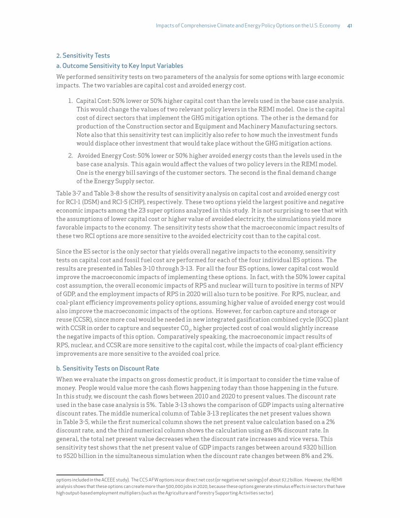
Impacts of Comprehensive Climate and Energy Policy Options on the U.S. Economy !41
2. Sensitivity Testsa. Outcome Sensitivity to Key Input VariablesWe performed sensitivity tests on two parameters of the analysis for some options with large economic impacts. The two variables are capital cost and avoided energy cost.
1.-Capital Cost: 50% lower or 50% higher capital cost than the levels used in the base case analysis. This would change the values of two relevant policy levers in the REMI model. One is the capital cost of direct sectors that implement the GHG mitigation options. The other is the demand for production of the Construction sector and Equipment and Machinery Manufacturing sectors. Note also that this sensitivity test can implicitly also refer to how much the investment funds would displace other investment that would take place without the GHG mitigation actions.
2.- Avoided Energy Cost: 50% lower or 50% higher avoided energy costs than the levels used in the base case analysis. This again would a!ect the values of two policy levers in the REMI model. One is the energy bill savings of the customer sectors. The second is the final demand change of the Energy Supply sector.
Table 3-7 and Table 3-8 show the results of sensitivity analysis on capital cost and avoided energy cost for RCI-1 (DSM) and RCI-5 (CHP), respectively. These two options yield the largest positive and negative economic impacts among the 23 super options analyzed in this study. It is not surprising to see that with the assumptions of lower capital cost or higher value of avoided electricity, the simulations yield more favorable impacts to the economy. The sensitivity tests show that the macroeconomic impact results of these two RCI options are more sensitive to the avoided electricity cost than to the capital cost.
Since the ES sector is the only sector that yields overall negative impacts to the economy, sensitivity tests on capital cost and fossil fuel cost are performed for each of the four individual ES options. The results are presented in Tables 3-10 through 3-13. For all the four ES options, lower capital cost would improve the macroeconomic impacts of implementing these options. In fact, with the 50% lower capital cost assumption, the overall economic impacts of RPS and nuclear will turn to positive in terms of NPV of GDP, and the employment impacts of RPS in 2020 will also turn to be positive. For RPS, nuclear, and coal-plant e$ciency improvements policy options, assuming higher value of avoided energy cost would also improve the macroeconomic impacts of the options. However, for carbon capture and storage or reuse (CCSR), since more coal would be needed in new integrated gasification combined cycle (IGCC) plant with CCSR in order to capture and sequester CO2, higher projected cost of coal would slightly increase the negative impacts of this option. Comparatively speaking, the macroeconomic impact results of RPS, nuclear, and CCSR are more sensitive to the capital cost, while the impacts of coal-plant e$ciency improvements are more sensitive to the avoided coal price.
b. Sensitivity Tests on Discount Rate When we evaluate the impacts on gross domestic product, it is important to consider the time value of money. People would value more the cash flows happening today than those happening in the future. In this study, we discount the cash flows between 2010 and 2020 to present values. The discount rate used in the base case analysis is 5%. Table 3-13 shows the comparison of GDP impacts using alternative discount rates. The middle numerical column of Table 3-13 replicates the net present values shown in Table 3-5, while the first numerical column shows the net present value calculation based on a 2% discount rate, and the third numerical column shows the calculation using an 8% discount rate. In general, the total net present value decreases when the discount rate increases and vice versa. This sensitivity test shows that the net present value of GDP impacts ranges between around $320 billion to $520 billion in the simultaneous simulation when the discount rate changes between 8% and 2%.
options included in"the ACEEE study)." The CCS AFW options incur direct net cost (or negative net savings) of about $7.2 billion." However, the REMI analysis shows that these options can create more than 500,000 jobs in 2020, because these options generate stimulus e#ects in sectors that have high output-based employment multipliers (such as the Agriculture and Forestry Supporting Activities sector).
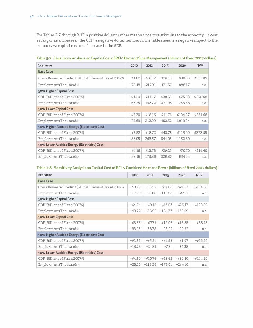
42!Johns Hopkins University and Center for Climate Strategies
For Tables 3-7 through 3-13, a positive dollar number means a positive stimulus to the economy — a cost saving or an increase in the GDP; a negative dollar number in the tables means a negative impact to the economy—a capital cost or a decrease in the GDP.
Table 3-7. Sensitivity Analysis on Capital Cost of RCI-1 Demand Side Management (billions of fixed 2007 dollars)
Scenarios 2010 2012 2015 2020 NPV
Base Case
Gross Domestic Product (GDP) (Billions of Fixed 2007$) $4.82 $16.17 $36.19 $90.05 $305.05
Employment (Thousands) 72.48 217.91 431.67 886.17 n.a.
50% Higher Capital Cost
GDP (Billions of Fixed 2007$) $4.29 $14.17 $30.63 $75.93 $258.68
Employment (Thousands) 66.25 193.72 371.08 753.88 n.a.
50% Lower Capital Cost
GDP (Billions of Fixed 2007$) $5.30 $18.16 $41.76 $104.27 $351.66
Employment (Thousands) 78.69 242.09 492.52 1,019.34 n.a.
50% Higher Avoided Energy (Electricity) Cost
GDP (Billions of Fixed 2007$) $5.52 $18.72 $43.78 $113.09 $373.55
Employment (Thousands) 86.95 263.67 544.05 1,152.30 n.a.
50% Lower Avoided Energy (Electricity) Cost
GDP (Billions of Fixed 2007$) $4.16 $13.73 $29.25 $70.70 $244.60
Employment (Thousands) 58.16 173.36 326.30 654.64 n.a.
Table 3-8. Sensitivity Analysis on Capital Cost of RCI-5 Combined Heat and Power (billions of fixed 2007 dollars)
Scenarios 2010 2012 2015 2020 NPV
Base Case
Gross Domestic Product (GDP) (Billions of Fixed 2007$) –$3.79 –$8.57 –$14.08 –$21.17 –$104.38
Employment (Thousands) –37.05 –78.88 –113.98 –127.91 n.a.
50% Higher Capital Cost
GDP (Billions of Fixed 2007$) –$4.04 –$9.43 –$16.07 –$25.47 –$120.29
Employment (Thousands) –40.22 –88.92 –134.77 –165.09 n.a.
50% Lower Capital Cost
GDP (Billions of Fixed 2007$) –$3.55 –$7.71 –$12.06 –$16.85 –$88.45
Employment (Thousands) –33.95 –68.78 –93.20 –90.52 n.a.
50% Higher Avoided Energy (Electricity) Cost
GDP (Billions of Fixed 2007$) –$2.39 –$5.24 –$4.98 $1.07 –$26.60
Employment (Thousands) –13.75 –24.81 –7.31 84.38 n.a.
50% Lower Avoided Energy (Electricity) Cost
GDP (Billions of Fixed 2007$) –$4.69 –$10.76 –$18.62 –$32.40 –$144.29
Employment (Thousands) –53.70 –113.58 –173.61 –244.16 n.a.

Impacts of Comprehensive Climate and Energy Policy Options on the U.S. Economy !43
Table 3-9. Sensitivity Analysis on Capital Cost of ES-1 Renewable Portfolio Standard (billions of fixed 2007 dollars)
Scenarios 2010 2012 2015 2020 NPV
Base Case
Gross Domestic Product (GDP) (Billions of Fixed 2007$) –$0.25 –$2.27 –$5.32 –$5.35 –$35.52
Employment (Thousands) 0.44 –21.42 –52.73 –58.61 n.a.
50% Higher Capital Cost
GDP (Billions of Fixed 2007$) –$0.69 –$4.23 –$9.93 –$16.61 –$73.69
Employment (Thousands) –5.59 –44.33 –99.56 –153.20 n.a.
50% Lower Capital Cost
GDP (Billions of Fixed 2007$) $0.19 –$0.31 –$0.62 $6.33 $3.75
Employment (Thousands) 6.39 1.39 –5.00 39.31 n.a.
50% Higher Avoided Energy (Coal and Natural Gas) Cost
GDP (Billions of Fixed 2007$) $0.04 –$1.50 –$2.93 $6.31 –$8.91
Employment (Thousands) 4.63 –13.63 –34.50 22.27 n.a.
50% Lower Avoided Energy (Coal and Natural Gas) Cost
GDP (Billions of Fixed 2007$) –$1.25 –$3.80 –$7.00 –$12.05 –$53.56
Employment (Thousands) –14.39 –42.41 –73.45 –112.22 n.a.
Table 3–10. Sensitivity Analysis on Capital Cost of ES–2 Nuclear (billions of fixed 2007 dollars)
Scenarios 2010 2012 2015 2020 NPV
Base Case
Gross Domestic Product (GDP) (Billions of Fixed 2007$) $0.00 –$0.07 –$0.46 –$6.85 –$8.14
Employment (Thousands) 0.00 –0.69 –5.08 –73.34 n.a.
50% Higher Capital Cost
GDP (Billions of Fixed 2007$) $0.00 –$0.20 –$1.01 –$12.75 –$17.36
Employment (Thousands) 0.00 –2.06 –10.48 –123.41 n.a.
50% Lower Capital Cost
GDP (Billions of Fixed 2007$) $0.00 $0.06 $0.08 –$0.83 $1.10
Employment (Thousands) 0.00 0.66 0.31 –22.20 n.a.
50% Higher Avoided Energy (Coal and Natural Gas) Cost
GDP (Billions of Fixed 2007$) $0.00 $0.05 –$0.10 –$2.35 –$1.24
Employment (Thousands) 0.00 0.53 –1.64 –35.67 n.a.
50% Lower Avoided Energy (Coal and Natural Gas) Cost
GDP (Billions of Fixed 2007$) $0.00 –$0.18 –$0.82 –$11.20 –$14.91
Employment (Thousands) 0.00 –1.94 –8.45 –109.75 n.a.
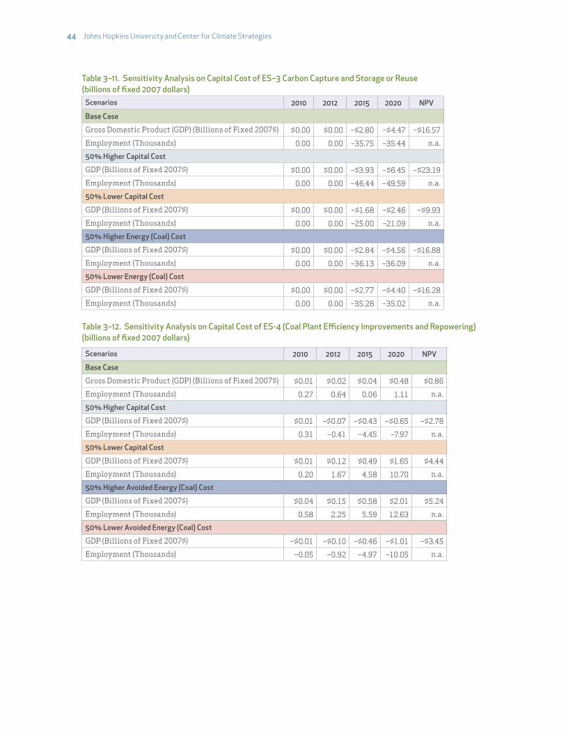
44!Johns Hopkins University and Center for Climate Strategies
Table 3–11. Sensitivity Analysis on Capital Cost of ES–3 Carbon Capture and Storage or Reuse (billions of fixed 2007 dollars)
Scenarios 2010 2012 2015 2020 NPV
Base Case
Gross Domestic Product (GDP) (Billions of Fixed 2007$) $0.00 $0.00 –$2.80 –$4.47 –$16.57
Employment (Thousands) 0.00 0.00 –35.75 –35.44 n.a.
50% Higher Capital Cost
GDP (Billions of Fixed 2007$) $0.00 $0.00 –$3.93 –$6.45 –$23.19
Employment (Thousands) 0.00 0.00 –46.44 –49.59 n.a.
50% Lower Capital Cost
GDP (Billions of Fixed 2007$) $0.00 $0.00 –$1.68 –$2.46 –$9.93
Employment (Thousands) 0.00 0.00 –25.00 –21.09 n.a.
50% Higher Energy (Coal) Cost
GDP (Billions of Fixed 2007$) $0.00 $0.00 –$2.84 –$4.56 –$16.88
Employment (Thousands) 0.00 0.00 –36.13 –36.09 n.a.
50% Lower Energy (Coal) Cost
GDP (Billions of Fixed 2007$) $0.00 $0.00 –$2.77 –$4.40 –$16.28
Employment (Thousands) 0.00 0.00 –35.28 –35.02 n.a.
Table 3–12. Sensitivity Analysis on Capital Cost of ES-4 (Coal Plant E$ciency Improvements and Repowering) (billions of fixed 2007 dollars)
Scenarios 2010 2012 2015 2020 NPV
Base Case
Gross Domestic Product (GDP) (Billions of Fixed 2007$) $0.01 $0.02 $0.04 $0.48 $0.86
Employment (Thousands) 0.27 0.64 0.06 1.11 n.a.
50% Higher Capital Cost
GDP (Billions of Fixed 2007$) $0.01 –$0.07 –$0.43 –$0.65 –$2.78
Employment (Thousands) 0.31 –0.41 –4.45 –7.97 n.a.
50% Lower Capital Cost
GDP (Billions of Fixed 2007$) $0.01 $0.12 $0.49 $1.65 $4.44
Employment (Thousands) 0.20 1.67 4.58 10.70 n.a.
50% Higher Avoided Energy (Coal) Cost
GDP (Billions of Fixed 2007$) $0.04 $0.15 $0.58 $2.01 $5.24
Employment (Thousands) 0.58 2.25 5.59 12.63 n.a.
50% Lower Avoided Energy (Coal) Cost
GDP (Billions of Fixed 2007$) –$0.01 –$0.10 –$0.46 –$1.01 –$3.45
Employment (Thousands) –0.05 –0.92 –4.97 –10.05 n.a.

Impacts of Comprehensive Climate and Energy Policy Options on the U.S. Economy !45
Table 3-13. Comparing Net Present Values with Alternative Discount Rates (billions of fixed 2007 dollars)
Policy Options
Discount Rate (NPV)
2% 5% 8% ES–1 Renewable Portfolio Standard –$43.88 –$35.52 –$29.07
ES–2 Nuclear –$10.75 –$8.14 –$6.23
ES=3 Carbon Capture and Storage or Reuse (CCSR) –$20.86 –$16.57 –$13.31
ES–4 Coal Plant E$ciency Improvements $1.10 $0.86 $0.67
Subtotal – ES –$74.40 –$59.38 –$47.94RCI–1 Demand Side Management Programs $382.64 $305.05 $246.18
RCI–2 High Performance Buildings $50.43 $40.14 $32.35
RCI–3 Appliance Standards –$0.51 –$0.43 –$0.36
RCI–4 Building Codes $61.34 $49.05 $39.71
RCI–5 Combined Heat and Power –$127.76 –$104.38 –$86.36
Subtotal – RCI $366.14 $289.44 $231.52
AFW–1 Crop Production Practices $21.84 $17.50 $14.18
AFW–2 Livestock Manure –$0.74 –$0.58 –$0.48
AFW–3 Forest Retention $4.18 $3.45 $2.87
AFW–4 Reforestation/A!orestation –$88.10 –$73.47 –$62.05
AFW–5 Urban Forestry $48.07 $40.12 $33.87
AFW–6 Source Reduction $12.94 $10.37 $8.41
AFW–7 Enhanced Recycling of MSW $63.57 $51.61 $42.40
AFW–8 MSW Landfill Gas Management $33.17 $26.47 $21.41
Subtotal – AFW $94.93 $75.46 $60.62
TLU–1 Vehicle Purchase Incentives $51.12 $39.64 $31.08
TLU–2 Renewable Fuel Standard –$21.68 –$17.08 –$13.59
TLU–3 Smart Growth $24.64 $19.54 $15.68
TLU–4 Transit $3.22 $2.46 $1.90
TLU–5 Anti–Idling Technologies and Practices $3.93 $2.96 $2.26
TLU–6 Mode Shi# from Truck to Rail $5.62 $2.92 $1.06
Subtotal –TLU $66.85 $50.45 $38.38
Summation Total $453.53 $355.97 $282.59
Simultaneous Total $520.74 $406.74 $321.29
MSW = municipal solid waste; NPV = net present value; ES = Energy Supply; RCI = Residential, Commercial, and Industrial; AFW = Agriculture, Forestry, and Waste Management; TLU = Transportation and Land Use.Note: A positive dollar number in the tables above means a positive stimulus to the economy – a cost saving or an increase in the GDP; a negative dollar number means a negative impact to the economy – a capital cost or a decrease in the GDP.
VII. Current Legislation The Kerry-Lieberman bill (K-L, 2010) has the following major features:
1.-Emission Caps: The emission caps for the covered sources are specified as 95.25% of the 2005 level in 2013; 83% of the 2005 level in 2020; 58% of the 2005 level in 2030; and 17% of the 2005 level in 2050 (i.e., 4.75%, 17%, 42%, and 83% below the 2005 level in 2013, 2020, 2030, and 2050, respectively).
2.-Covered Sectors and Phase-in Schedule: Starting in 2013, the Electric Power sector and Refined Petroleum Products Manufacturing sector will be covered by the cap. Starting in 2016, the Industrial sector (for entities that emit > 25,000 tons of CO2 equivalent from either fuel combustion or industrial processes) and the Natural Gas Distribution sector will be covered by the cap. Entities covered by the cap a#er year 2016 collectively contribute about 85% of gross GHG emissions in the U.S. (Doniger, 2010).

46!Johns Hopkins University and Center for Climate Strategies
3.-Allowance Price: The reserve price of an allowance at auction will be set at $12 per ton (2009$) starting in 2013, and this price will increase at the rate of inflation (as measured by the CPI) plus 3% for each year a#erwards. The allowance price of the cost containment reserve will be set at $25 per ton (2009$) starting in 2013 and will increase at the rate of inflation (as measured by the CPI) plus 5% for each year a#erwards. In our simulation cases, we will determine the allowance price internally based on the U.S. marginal mitigation cost curve developed in Section 2. Where this approach will not yield a reasonable allowance price (such as in the Stakeholder Full Implementation scenario), we will use the reserve price to compute the auction payments/revenues.
4.-Banking and Borrowing: The bill allows unlimited banking. The bill will also establish a two-year rolling compliance period that allows the covered entities to borrow an unlimited number of allowances from one year into the future. However, they need to pay back the borrowed allowances in the second year to avoid any penalty. Covered entities can also use future five years’ allowances for up to 15% of current year compliance with an 8% penalty.
5.-O!sets: O!set credits can be used to achieve compliance for up to a maximum of 2 billion tons of GHG emissions annually. In general, the limit on the use of international o!set credits is 0.5 billion tons. However, if the use of domestic o!sets is less than 1.5 billion tons, the limit on the international o!set credits can be increased to a maximum of 1 billion tons. In addition, covered entities can use 1 domestic o!set credit or 1.25 international o!set credits to demonstrate compliance. In our analysis, the domestic o!set price is determined endogenously based on the cost curve of the methane and forestry mitigation options from the Agricultural, Forestry, and Waste sector.
6.-Disposition of Allowances and Auction Percentage: Table 1 summarizes the use of auction revenues and is based on the provisions specified in Sec. 2101 of the K-L bill. The disposition of the allowances to di!erent sectors and objectives are summarized for three key years within the study period of our analysis (years 2013, 2015, and 2020). The table is divided into two sections. The first section lists the direct (free) allocation of the allowances. The second section lists the allowances distribution through the spending of auction proceeds.
7.-Auction Revenue Recycling: According to Table 1, the auction proceeds will be devoted to “Consumer Relief,” “Universal Trust Fund,” “Highway Trust Fund,” and “Deficit Reduction Fund.” The consumer relief program includes the working families refundable credit program and the energy refund program. For the working families refundable credit program, an eligible taxpayer is defined as an individual whose household income is less than 150% of the poverty line minus $1,000. For the energy refund program, there are many criteria to define an eligible household, such as a household that has income less than 150% of the poverty line, that is participating in the Supplemental Nutrition Assistant Program, Food Distribution Program, etc. In our simulation, we will use the 150 percent federal poverty level to define the household income group that will be covered by consumer relief programs. In addition, all households are likely eligible for the “Universal Trust Fund.” However, this fund will not be established until 2026, and, therefore, it will not be simulated in our analysis.

Impacts of Comprehensive Climate and Energy Policy Options on the U.S. Economy !47
Table 3-14. Allowance Allocation Scheme of the K-L Bill (based on Section 2101)
Allowance Allocation Schemes 2013 2015 2020 CCS SectorsDirect Allocation of Allowances # # #Electricity Consumers (first distributed to local distribution companies) 51.0% 51.0% 35.0% ES
Natural Gas Consumers (first distributed to local distribution companies) 0.0% 0.0% 9.0%
Res, Com, Ind-EIS, and Ind-Other
Home Heating Oil and Propane Consumers (first distributed to states) 1.9% 1.9% 1.5% Res
Trade-exposed Industries 2.0% 2.0% 15.0% Ind-EIS
Industrial Energy E$ciency 0.5% 0.5% 0.0% Ind-EIS and Ind-Other
Refiners 4.3% 4.3% 3.8% Ind-Other
Deployment of Carbon Capture and Sequestration Technology 0.0% 0.0% 4.5% ES
Clean Vehicle Technology 1.0% 1.0% 1.0% TLU
Low-carbon Industrial Technologies Research and Development 1.0% 1.0% 1.0% Com (R&D sector)
Clean Energy Technology Research and Development 2.0% 2.0% 2.0% Com (R&D sector)
Investment in Energy E$ciency and Renewable Energy 2.5% 2.5% 1.0%
Split between ES, Ind-EIS, Ind-Other, and Com sectors
Early Action 1.0% 1.0% 0.0%
Split between ES, Ind-EIS, Ind-Other, and Com sectors
National Surface Transportation System 4.0% 4.0% 2.0% TLU
Investment in Transportation GHG Emission Reduction Programs 4.0% 4.0% 2.0%
Ind-Other (auto manufacturing and refiner sectors)
Total Free Allocation Percentage 75.2% 75.2% 78.8%Adaptation (1/2 to domestic adaptation and 1/2 to international adaptation)a 0.0% 0.0% 1.5%
Distribution of Spending of Allowance Auction Proceeds # # #Consumer Relief 12.3% 12.3% 10.6%
Universal Trust Fund 0.0% 0.0% 0.0%
Highway Trust Fund 4.0% 4.0% 2.0%
Deficit Reduction Fund 8.5% 8.5% 8.1%
Total Auction Percentage 24.8% 24.8% 20.8% Notes: ES = Electricity Supply sector; Res = Residential sector; Com = Commercial sector; Ind-EIS = Energy-Intensive Industrial sector; Ind-Other = Other Industrial sector; R&D = research and development; TLU = Transportation sector. a Allowances to adaptation will not be simulated as allowance distribution to any capped sectors; instead, we will simulate it as a lump-sum payment to state and local government for domestic adaptation and as a foreign transfer for international adaptation.
VIII. Analysis of the Senate Bill 1. Scenario 1. Stakeholder Recommendation CaseThis is the implementation of all mitigation options presented in Table 3-15 as described in Subsection VI above. This scenario excludes consideration of major features of the K-L bill.

48!Johns Hopkins University and Center for Climate Strategies
Table 3-15. 2020 GHG Reduction Potentials and Cost-E"ectiveness of 23 GHG Mitigation “Super Options” for the U.S., 2020
Sector Climate Mitigation Actions
Estimated 2020
Annual GHG Reduction Potential
(MMtCO2e)
Estimated Cost or Cost Savings per
Ton GHG Removed ($)
GHG Reduction
Potential as Percentage
of 2020 Baseline
Emissions
Cumulative GHG
Reduction Potentials
Price-Responsive
Options
TLU-6 Mode Shi# from Truck to Rail 36.85 –$91.56 0.48% 0.48% No
TLU-1 Vehicle Purchase Incentives, Including Rebates 103.07 –$66.37 1.34% 1.82% Yes
TLU-5 Anti-Idling Technologies and Practices 33.82 –$65.19 0.44% 2.26% No
RCI-3 Appliance Standards 80.86 –$53.21 1.05% 3.31% No
RCI-1 Demand Side Management Programs 424.80 –$40.71 5.52% 8.83%
30% of the emission reductions are price-responsive
RCI-2 High Performance Buildings (Private and Public Sector) 193.88 –$24.99 2.52% 11.35%
30% of the emission reductions are price-responsive
RCI-4 Building Codes 161.08 –$22.86 2.09% 13.44% No
AFW-1 Crop Production Practices to Achieve GHG Benefits 65.01 –$15.69 0.84% 14.29%
50% of the emission reductions are price-responsive
RCI-5 Combined Heat and Power 136.37 –$13.18 1.77% 16.06%
30% of the emission reductions are price-responsive
AFW-6 MSW Source Reduction 147.09 –$3.20 1.91% 17.97% NoTLU-3 Smart Growth/Land Use 71.04 –$1.11 0.92% 18.89% NoAFW-8 MSW Landfill Gas Management 48.38 $0.34 0.63% 19.52% Yes
AFW-2Livestock Manure – Anaerobic Digestion and Methane Utilization
19.25 $11.27 0.25% 19.77% Yes
ES-4 Coal Plant E$ciency Improvements and Repowering 151.05 $12.95 1.96% 21.74% Yes
AFW-7 Enhanced Recycling of Municipal Solid Waste 249.27 $13.39 3.24% 24.97% No
AFW-5 Urban Forestry 39.96 $15.35 0.52% 25.49% YesTLU-4 Transit 27.05 $16.72 0.35% 25.85% NoES-1 Renewable Portfolio Standard 508.39 $17.84 6.61% 32.45% No
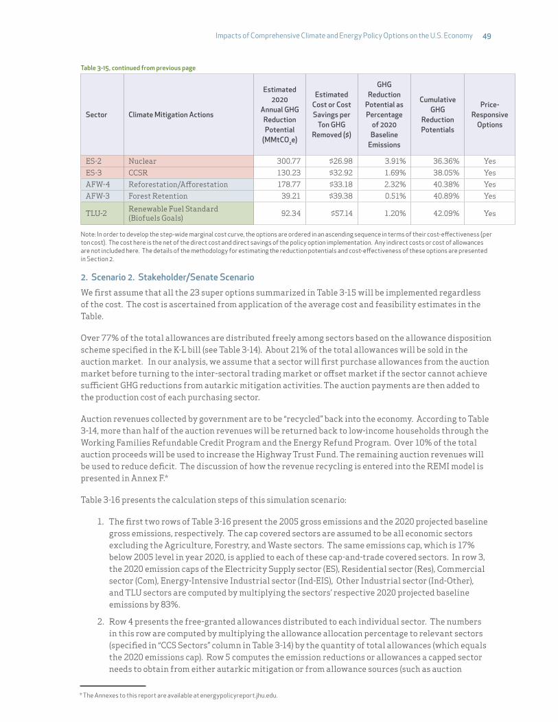
Impacts of Comprehensive Climate and Energy Policy Options on the U.S. Economy !49
Sector Climate Mitigation Actions
Estimated 2020
Annual GHG Reduction Potential
(MMtCO2e)
Estimated Cost or Cost Savings per
Ton GHG Removed ($)
GHG Reduction
Potential as Percentage
of 2020 Baseline
Emissions
Cumulative GHG
Reduction Potentials
Price-Responsive
Options
ES-2 Nuclear 300.77 $26.98 3.91% 36.36% YesES-3 CCSR 130.23 $32.92 1.69% 38.05% YesAFW-4 Reforestation/A!orestation 178.77 $33.18 2.32% 40.38% YesAFW-3 Forest Retention 39.21 $39.38 0.51% 40.89% Yes
TLU-2 Renewable Fuel Standard (Biofuels Goals) 92.34 $57.14 1.20% 42.09% Yes
Note: In order to develop the step-wide marginal cost curve, the options are ordered in an ascending sequence in terms of their cost-e#ectiveness (per ton cost). The cost here is the net of the direct cost and direct savings of the policy option implementation. Any indirect costs or cost of allowances are not included here. The details of the methodology for estimating the reduction potentials and cost-e#ectiveness of these options are presented in Section 2.
2. Scenario 2. Stakeholder/Senate ScenarioWe first assume that all the 23 super options summarized in Table 3-15 will be implemented regardless of the cost. The cost is ascertained from application of the average cost and feasibility estimates in the Table.
Over 77% of the total allowances are distributed freely among sectors based on the allowance disposition scheme specified in the K-L bill (see Table 3-14). About 21% of the total allowances will be sold in the auction market. In our analysis, we assume that a sector will first purchase allowances from the auction market before turning to the inter-sectoral trading market or o!set market if the sector cannot achieve su$cient GHG reductions from autarkic mitigation activities. The auction payments are then added to the production cost of each purchasing sector.
Auction revenues collected by government are to be “recycled” back into the economy. According to Table 3-14, more than half of the auction revenues will be returned back to low-income households through the Working Families Refundable Credit Program and the Energy Refund Program. Over 10% of the total auction proceeds will be used to increase the Highway Trust Fund. The remaining auction revenues will be used to reduce deficit. The discussion of how the revenue recycling is entered into the REMI model is presented in Annex F.*
Table 3-16 presents the calculation steps of this simulation scenario:
1. The first two rows of Table 3-16 present the 2005 gross emissions and the 2020 projected baseline gross emissions, respectively. The cap covered sectors are assumed to be all economic sectors excluding the Agriculture, Forestry, and Waste sectors. The same emissions cap, which is 17% below 2005 level in year 2020, is applied to each of these cap-and-trade covered sectors. In row 3, the 2020 emission caps of the Electricity Supply sector (ES), Residential sector (Res), Commercial sector (Com), Energy-Intensive Industrial sector (Ind-EIS), Other Industrial sector (Ind-Other), and TLU sectors are computed by multiplying the sectors’ respective 2020 projected baseline emissions by 83%.
2. Row 4 presents the free-granted allowances distributed to each individual sector. The numbers in this row are computed by multiplying the allowance allocation percentage to relevant sectors (specified in “CCS Sectors” column in Table 3-14) by the quantity of total allowances (which equals the 2020 emissions cap). Row 5 computes the emission reductions or allowances a capped sector needs to obtain from either autarkic mitigation or from allowance sources (such as auction
Table 3-15, continued from previous page
* The Annexes to this report are available at energypolicyreport.jhu.edu.

50!Johns Hopkins University and Center for Climate Strategies
market, inter-sectoral trading market, or o!set market). This is computed as the di!erence between the 2020 baseline emission of a sector (row 2) and the free allocated allowances to this sector (row 4). Please note the numbers for the Commercial sector and the Energy-Intensive Industrial sector in this row are negative. This means according to our calculation, these two sectors will receive more free allowances than their projected baseline emissions.
3. Row 6 presents the reductions that can be achieved from the full implementation of the CCS options in the respective sectors. The total e!orts of the 23 super options can help reduce the 2020 baseline emissions by 42.09%.
4. Row 7 computes the allowances each sector purchases from auction. The values are zero for the ES sector and Residential sector because their respective reductions from mitigation (row 6) are greater than the emissions reductions or allowances they need to obtain as indicated in row 5. The values are zero for the Commercial sector and the Energy-Intensive Industrial sector because they even get free allowances above their baseline emissions. Ind-Other and TLU are the only two sectors that need to purchase allowances a#er their own-source mitigation. The number for the Ind-Other sector is computed as the di!erence between the reductions and allowances this sector needs (row 5) and the mitigation this sector can achieve from implementing sectoral mitigation options (row 6). The allowances the TLU sector will buy from the auction market is computed as the residual of the total allowances available in the auction market and the allowances purchased by the Ind-Other sector from the auction market. Comparing the numbers in rows 5 to 7 in the TLU column, we can see that the TLU sector cannot acquire enough reductions from TLU mitigation and the auction market (row 6 + row 7 < row 5).
5. In row 8, we compute the allowances transactions in the inter-sectoral trading market. Since Scenario 2 assumes that the 23 super options will be fully implemented under regulations, even though many sectors will achieve over-compliance, they cannot sell the excess reductions to the other sectors. Therefore, we assume in this step that only the free-allocated allowances that exceed the baseline emissions of a sector will be sold to the other sectors. Thus, the TLU sector can buy 11 million tons of allowances from the Commercial sector and 368 million tons from the Ind-EIS sector.
6. Domestic o!sets will not be available in this scenario since all sectors are “covered” by either cap and trade or other policies and measures. Therefore, the numbers in row 9 are all zero.
7. The remaining need for allowances of the TLU sector is then assumed to be achieved from purchasing allowances from the international o!set market. Since 1.25 tons of international o!set credits are needed for 1 ton of emissions, a factor of 1.25 is applied to get the total international o!sets purchased in tons in row 10. The o!set price is assumed to be same as the allowance price.
8. Row 11 computes the allowances banking by sector. Based on all the above assumptions, no allowances are available for banking in this scenario.
The macroeconomic impacts and its decomposition of the Stakeholder/Senate scenario 2 are presented in Table 3-17. The overall impacts of this simulation case are projected to be a $116.9 billion increase in GDP (or a 0.68% increase from the baseline level) and a 2.13 million increase in employment (or a 1.15% increase from the baseline level) in 2020. The decomposition of the results is as follows:
"» Implementation of the 23 super options will increase GDP by $159.5 billion and create 2.5 million more jobs in 2020. These reflect the total impacts of the 23 super options implemented simultaneously.
"» Production cost increase of the Ind-Other and TLU sectors due to the purchases of allowances in the auction market will cause a decrease in GDP of $43.0 billion and a decrease in employment of 432,000.
"» Recycling of the auction revenue would generate an increase in GDP of $19.0 billion and an increase in employment of 240,000.
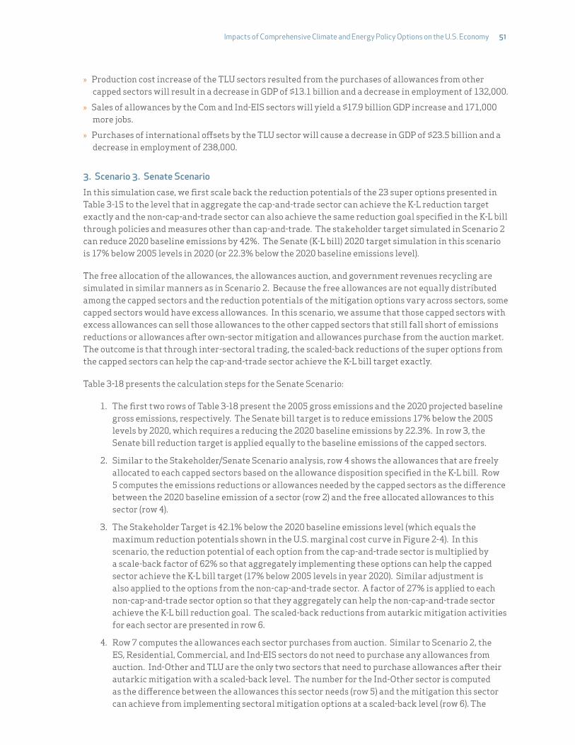
Impacts of Comprehensive Climate and Energy Policy Options on the U.S. Economy !51
"» Production cost increase of the TLU sectors resulted from the purchases of allowances from other capped sectors will result in a decrease in GDP of $13.1 billion and a decrease in employment of 132,000.
"» Sales of allowances by the Com and Ind-EIS sectors will yield a $17.9 billion GDP increase and 171,000 more jobs.
"» Purchases of international o!sets by the TLU sector will cause a decrease in GDP of $23.5 billion and a decrease in employment of 238,000.
3. Scenario 3. Senate ScenarioIn this simulation case, we first scale back the reduction potentials of the 23 super options presented in Table 3-15 to the level that in aggregate the cap-and-trade sector can achieve the K-L reduction target exactly and the non-cap-and-trade sector can also achieve the same reduction goal specified in the K-L bill through policies and measures other than cap-and-trade. The stakeholder target simulated in Scenario 2 can reduce 2020 baseline emissions by 42%. The Senate (K-L bill) 2020 target simulation in this scenario is 17% below 2005 levels in 2020 (or 22.3% below the 2020 baseline emissions level).
The free allocation of the allowances, the allowances auction, and government revenues recycling are simulated in similar manners as in Scenario 2. Because the free allowances are not equally distributed among the capped sectors and the reduction potentials of the mitigation options vary across sectors, some capped sectors would have excess allowances. In this scenario, we assume that those capped sectors with excess allowances can sell those allowances to the other capped sectors that still fall short of emissions reductions or allowances a#er own-sector mitigation and allowances purchase from the auction market. The outcome is that through inter-sectoral trading, the scaled-back reductions of the super options from the capped sectors can help the cap-and-trade sector achieve the K-L bill target exactly.
Table 3-18 presents the calculation steps for the Senate Scenario:
1. The first two rows of Table 3-18 present the 2005 gross emissions and the 2020 projected baseline gross emissions, respectively. The Senate bill target is to reduce emissions 17% below the 2005 levels by 2020, which requires a reducing the 2020 baseline emissions by 22.3%. In row 3, the Senate bill reduction target is applied equally to the baseline emissions of the capped sectors.
2. Similar to the Stakeholder/Senate Scenario analysis, row 4 shows the allowances that are freely allocated to each capped sectors based on the allowance disposition specified in the K-L bill. Row 5 computes the emissions reductions or allowances needed by the capped sectors as the di!erence between the 2020 baseline emission of a sector (row 2) and the free allocated allowances to this sector (row 4).
3. The Stakeholder Target is 42.1% below the 2020 baseline emissions level (which equals the maximum reduction potentials shown in the U.S. marginal cost curve in Figure 2-4). In this scenario, the reduction potential of each option from the cap-and-trade sector is multiplied by a scale-back factor of 62% so that aggregately implementing these options can help the capped sector achieve the K-L bill target (17% below 2005 levels in year 2020). Similar adjustment is also applied to the options from the non-cap-and-trade sector. A factor of 27% is applied to each non-cap-and-trade sector option so that they aggregately can help the non-cap-and-trade sector achieve the K-L bill reduction goal. The scaled-back reductions from autarkic mitigation activities for each sector are presented in row 6.
4. Row 7 computes the allowances each sector purchases from auction. Similar to Scenario 2, the ES, Residential, Commercial, and Ind-EIS sectors do not need to purchase any allowances from auction. Ind-Other and TLU are the only two sectors that need to purchase allowances a#er their autarkic mitigation with a scaled-back level. The number for the Ind-Other sector is computed as the di!erence between the allowances this sector needs (row 5) and the mitigation this sector can achieve from implementing sectoral mitigation options at a scaled-back level (row 6). The

52!Johns Hopkins University and Center for Climate Strategies
allowances the TLU sector will buy from the auction market is computed as the residual of the total allowances available in the auction market and the allowances purchased by the Ind-Other sector from the auction market. Comparing the numbers in rows 5 to 7 in the TLU column, we can see that the TLU sector cannot acquire enough reductions or allowances from its own mitigation and the auction market (row 6 + row 7 < row 5).
5. Row 8 computes the allowance transactions in the inter-sectoral trading market. Since the objective of this Scenario is that the proportional scaled-back reductions of the cap-and-trade sector mitigation options will enable the cap-and-trade sector to achieve the Senate bill target exactly, we assume that the capped sectors with excess emission reductions can sell the allowances to the TLU sector. The negative numbers in this row represent allowance selling and positive numbers represent allowance purchasing.
6. Domestic and international o!sets will not be needed in this scenario since the proportional scaled-back reductions of the cap-and-trade sector mitigation options will enable the cap-and-trade sector achieve the Senate bill target exactly.
7. Finally, no allowances can be banked since there are no excess allowances.
The macroeconomic impact and its decomposition of the Senate Scenario are presented in Table 3-19. The overall impacts of this simulation case are projected to be a $50.7 billion increase in GDP (or a 0.30% increase from the baseline level) and a 0.92 million increase in employment (or a 0.50% increase from the baseline level) in 2020. The decomposition of the results is as follows:
"» The scaled-back implementation of the 23 super options will increase GDP by $76.9 billion and create 1.15 million more jobs in 2020. These impacts are computed by applying the scale-back factor of 62% and 27% to the simultaneous impacts of the cap-and-trade sector options and the simultaneous impacts of the non-cap-and-trade sector options, respectively.
"» The production cost increase of the Ind-Other and TLU sectors due to the purchases of allowances in the auction market will cause a decrease in GDP of $43.6 billion and a decrease in employment of 438,000.
"» Recycling of the auction revenue would generate an increase in GDP of $19.0 billion and an increase in employment of 240,000.
"» The production cost increase of the TLU sectors resulted from the purchases of allowances from other capped sectors will result in a decrease in GDP of $33.7 billion and a decrease in employment of 341,000.
"» The sales of allowances by the Com and Ind-EIS sectors will yield a $32.1 billion GDP increase and 314,000 more jobs.
Several findings are summarized for a comparison of the Stakeholder/Senate Scenario results and the Senate Scenario results:
"» The Senate Scenario yields less positive impacts to the economy compared with the Stakeholder/Senate Scenario.
"» The major positive impacts in both scenarios come from the implementation of the 23 super options. As expected, with scaled-back e!orts of the 23 super options in the Senate Scenarios, the stimulus is lower.
"» In the Stakeholder/Senate Scenario, since the 23 super options will be implemented in full under regulations, we assume that a sector cannot sell its excess reductions achieved from mitigation to other sectors. In the Senate Scenario, we assume that the excess reductions can be traded among the capped sectors. Therefore, compared with the Stakeholder/Senate Scenario, there will be more allowances transactions among the capped sectors and no allowance purchases from the international o!set market in the Senate Scenario. Since the inter-sectoral trading will generate stimulus e!ects to the allowances selling sectors, while the international o!set purchases will be a pure out-flow of money to outside of the country, the Senate Scenario results in higher stimulus e!ects in the inter-sectoral trading aspect.
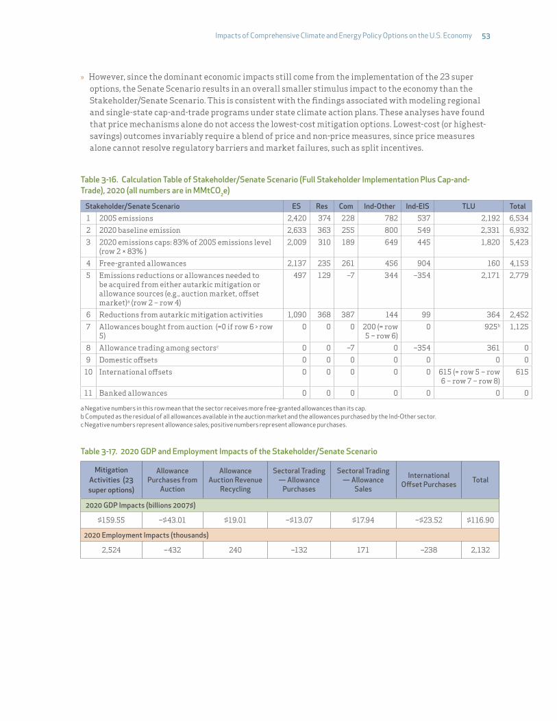
Impacts of Comprehensive Climate and Energy Policy Options on the U.S. Economy !53
"» However, since the dominant economic impacts still come from the implementation of the 23 super options, the Senate Scenario results in an overall smaller stimulus impact to the economy than the Stakeholder/Senate Scenario. This is consistent with the findings associated with modeling regional and single-state cap-and-trade programs under state climate action plans. These analyses have found that price mechanisms alone do not access the lowest-cost mitigation options. Lowest-cost (or highest-savings) outcomes invariably require a blend of price and non-price measures, since price measures alone cannot resolve regulatory barriers and market failures, such as split incentives.
Table 3-16. Calculation Table of Stakeholder/Senate Scenario (Full Stakeholder Implementation Plus Cap-and-Trade), 2020 (all numbers are in MMtCO2e)
#Stakeholder/Senate Scenario ES Res Com Ind-Other Ind-EIS TLU Total1 2005 emissions 2,420 374 228 782 537 2,192 6,534
2 2020 baseline emission 2,633 363 255 800 549 2,331 6,932
3 2020 emissions caps: 83% of 2005 emissions level (row 2 1 83% )
2,009 310 189 649 445 1,820 5,423
4 Free-granted allowances 2,137 235 261 456 904 160 4,153
5 Emissions reductions or allowances needed to be acquired from either autarkic mitigation or allowance sources (e.g., auction market, o!set market)a (row 2 – row 4)
497 129 –7 344 –354 2,171 2,779
6 Reductions from autarkic mitigation activities 1,090 368 387 144 99 364 2,452
7 Allowances bought from auction (=0 if row 6 > row 5)
0 0 0 200 (= row 5 – row 6)
0 925b 1,125
8 Allowance trading among sectorsc 0 0 –7 0 –354 361 0
9 Domestic o!sets 0 0 0 0 0 0 0
10 International o!sets 0 0 0 0 0 615 (= row 5 – row 6 – row 7 – row 8)
615
11 Banked allowances 0 0 0 0 0 0 0
a Negative numbers in this row mean that the sector receives more free-granted allowances than its cap. b Computed as the residual of all allowances available in the auction market and the allowances purchased by the Ind-Other sector.c Negative numbers represent allowance sales; positive numbers represent allowance purchases.
Table 3-17. 2020 GDP and Employment Impacts of the Stakeholder/Senate Scenario
Mitigation Activities (23 super options)
Allowance Purchases from
Auction
Allowance Auction Revenue
Recycling
Sectoral Trading — Allowance
Purchases
Sectoral Trading — Allowance
Sales
International O"set Purchases Total
2020 GDP Impacts (billions 2007$)
$159.55 –$43.01 $19.01 –$13.07 $17.94 –$23.52 $116.90
2020 Employment Impacts (thousands)
2,524 –432 240 –132 171 –238 2,132
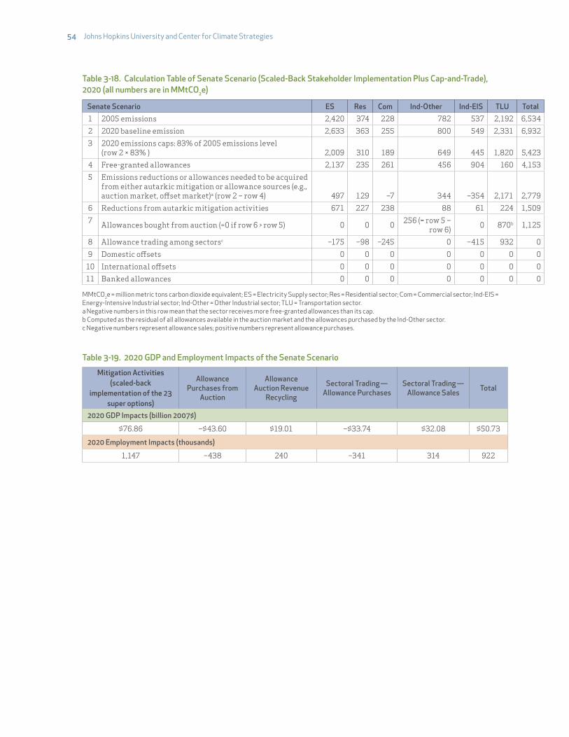
54!Johns Hopkins University and Center for Climate Strategies
Table 3-18. Calculation Table of Senate Scenario (Scaled-Back Stakeholder Implementation Plus Cap-and-Trade), 2020 (all numbers are in MMtCO2e)
#Senate Scenario ES Res Com Ind-Other Ind-EIS TLU Total1 2005 emissions 2,420 374 228 782 537 2,192 6,534
2 2020 baseline emission 2,633 363 255 800 549 2,331 6,932
3 2020 emissions caps: 83% of 2005 emissions level (row 2 1 83% ) 2,009 310 189 649 445 1,820 5,423
4 Free-granted allowances 2,137 235 261 456 904 160 4,153
5 Emissions reductions or allowances needed to be acquired from either autarkic mitigation or allowance sources (e.g., auction market, o!set market)a (row 2 – row 4) 497 129 –7 344 –354 2,171 2,779
6 Reductions from autarkic mitigation activities 671 227 238 88 61 224 1,509
7 Allowances bought from auction (=0 if row 6 > row 5) 0 0 0 256 (= row 5 – row 6) 0 870b 1,125
8 Allowance trading among sectorsc –175 –98 –245 0 –415 932 0
9 Domestic o!sets 0 0 0 0 0 0 0
10 International o!sets 0 0 0 0 0 0 0
11 Banked allowances 0 0 0 0 0 0 0
MMtCO2e = million metric tons carbon dioxide equivalent; ES = Electricity Supply sector; Res = Residential sector; Com = Commercial sector; Ind-EIS = Energy-Intensive Industrial sector; Ind-Other = Other Industrial sector; TLU = Transportation sector. a Negative numbers in this row mean that the sector receives more free-granted allowances than its cap. b Computed as the residual of all allowances available in the auction market and the allowances purchased by the Ind-Other sector. c Negative numbers represent allowance sales; positive numbers represent allowance purchases.
Table 3-19. 2020 GDP and Employment Impacts of the Senate Scenario
Mitigation Activities (scaled-back
implementation of the 23 super options)
Allowance Purchases from
Auction
Allowance Auction Revenue
Recycling
Sectoral Trading!—Allowance Purchases
Sectoral Trading!— Allowance Sales Total
2020 GDP Impacts (billion 2007$)
$76.86 –$43.60 $19.01 –$33.74 $32.08 $50.73
2020 Employment Impacts (thousands)
1,147 –438 240 –341 314 922

Impacts of Comprehensive Climate and Energy Policy Options on the U.S. Economy !55
State climate plans developed in the past decade were designed to develop comprehensive policy in all sectors, using all implementation tools at all appropriate levels of government (e.g. local, state, federal) in order to capture the broadest and most e!ective choices for low cost, high co-benefit solutions. Many of these policies were understandably focused on actions available to states and localities where federal jurisdiction was not applicable, or where federal willpower was lacking. But the recommendations are not restricted to state and local jurisdiction. Indeed, many policy options were viewed as more appropriate for federal or shared federal/state implementation. Nearly all state plans contain advisory or advocacy statements regarding the need for federal action for specific policy options and categories. O#en these statements are a preface to state or regional (multi-state) policy recommendations, and typically take the form,
“The Council strongly recommends that this state advocates for adoption of an aggressive federal [state policy type] program, as only a comprehensive national program can address all of the complexities associated with implementation of a single-state or regional plan. In the event the federal government does not take action or delays action in this area, we recommend the following. Should a federal program be established a"er the recommended program is in place, it is our recommendation that the program described here be discontinued.”
Jurisdictional issues are a major consideration in any comprehensive economy-wide climate plan. As seen in Sections 2 and 3, no single policy or action can achieve national or state reduction goals at acceptable cost levels. However, if done properly, a portfolio of measures across all sectors and employing a wide range of policy instruments can achieve reductions beyond national goals, strengthen the economy, and increase income.
The task of implementing this portfolio is no less complex than the diversity of measures it contains. Measures such as automobile emissions standards, threshold appliance or building e$ciency standards, renewable fuel standards, most market-based mechanisms such as cap-and-trade, and many others are clearly be"er suited to federal or shared federal/state implementation. Issues of boundary e!ects, equity and competitiveness are dramatically reduced or eliminated through this approach.
On the other hand, the state action plan portfolio also contains land use measures sometimes referred to as ‘location e$ciency’ and other action areas more applicable to state and local jurisdiction. The problems and opportunities for improved location e$ciency, for instance, vary from state to state and locality to locality. Likewise, opportunities for cost-e!ective transit policies vary dramatically based upon population density and historical development pa"erns. E!ective transit and location e$ciency climate policy measures need to be embraced and enacted by the levels of government with traditional jurisdiction over such ma"ers – local, metropolitan, and state. As a result, stakeholder representatives did not recommend national land use policies.
To be"er understand the jurisdictional issues of comprehensive climate action, the 23 super options were reclassified from their economic sectors to the level of government traditionally exercising sole, primary or shared jurisdiction. Authority over these policies varies from state to state, with some states exercising li"le or no control over local jurisdictional authority (typically “Home Rule” states),
%&'()*+ 2*3/
» Mitigation Option Implementation:Jurisdiction and Programmatic Issues

56!Johns Hopkins University and Center for Climate Strategies
while others may exercise a great deal (typically “Dillon’s Rule” states). The classifications used here are therefore generalized to show what is typical but by no means universal.
Figure 4-1 shows the breakdown of emissions reductions o!ered by full stakeholder implementation of the 23 super option policies by the level of government most likely to possess traditional jurisdiction.
Figure 4-1. Potential 2020 Emission Reductions by Government Level 2020 Stakeholder Implementation Potential GHG Emissions Reductions by Jurisdiction Source: Center for Climate Strategies, 2010.
SharedState/Federal
38%
Primary State31%
SharedLocal/State
28%
Primary Local 3%
Not surprisingly, much government authority is shared between levels, meaning either level typically has the authority to enact the policy or measure. Some examples of shared state and federal authority include agriculture incentive programs, waste management regulations and appliance standards. Shared state and local jurisdiction include smart growth, transit and building codes.
This analysis shows the importance of integrating local, state and federal actions, as well as policy instruments, to minimize costs and maximize co-benefits. For example:
"» 38% of total potential emissions reductions can be achieved through measures under shared federal and state jurisdiction;
"» 31% of potential emissions reductions can be achieved through measures primarily under state jurisdiction; and
"» 31% of potential emissions reductions can be achieved through measures primarily under local or shared local/state jurisdiction.
While the source of these data (state climate action plans) introduces some bias against exclusively federal policies (particularly due to the time period of federal recalcitrance in which they were developed), the role of the states and localities is undeniable. And the critical partner among the three levels of government appears to be the states; 97% of all emissions reductions are achievable by policies where the states have either primary or shared jurisdiction.
Of course, the underlying assumption here is that these 23 super policy options are implemented nationally, and while many states have led the nation in the design and implementation of climate programs, there is no immediate prospect that all 50 states will independently adopt such measures. The federal role in bringing about comprehensive and cost-e!ective climate action is clear. Equally clear from this study, however, is that only a national partnership among government levels can achieve the most comprehensive and economically beneficial reductions.
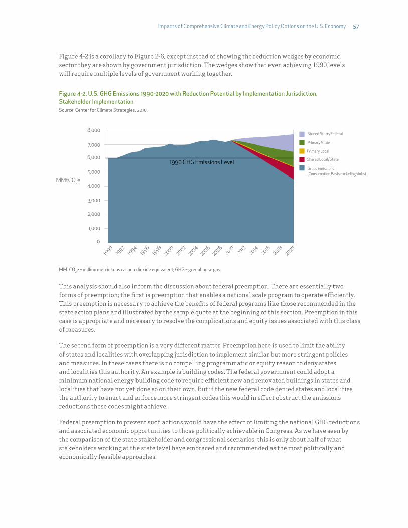
Impacts of Comprehensive Climate and Energy Policy Options on the U.S. Economy !57
Figure 4-2 is a corollary to Figure 2-6, except instead of showing the reduction wedges by economic sector they are shown by government jurisdiction. The wedges show that even achieving 1990 levels will require multiple levels of government working together.
Figure 4-2. U.S. GHG Emissions 1990-2020 with Reduction Potential by Implementation Jurisdiction, Stakeholder Implementation Source: Center for Climate Strategies, 2010.
Shared State/Federal
Primary State
Primary Local
Shared Local/State
Gross Emissions(Consumption Basis excluding sinks)
MMtCO2e
0
19901992
19941996
19982000
20022004
20062008
20102012
20142016
20182020
1,000
2,000
3,000
4,000
5,000
6,000
7,000
8,000
1990 GHG Emissions Level
MMtCO2e = million metric tons carbon dioxide equivalent; GHG = greenhouse gas.
This analysis should also inform the discussion about federal preemption. There are essentially two forms of preemption; the first is preemption that enables a national scale program to operate e$ciently. This preemption is necessary to achieve the benefits of federal programs like those recommended in the state action plans and illustrated by the sample quote at the beginning of this section. Preemption in this case is appropriate and necessary to resolve the complications and equity issues associated with this class of measures.
The second form of preemption is a very di!erent ma"er. Preemption here is used to limit the ability of states and localities with overlapping jurisdiction to implement similar but more stringent policies and measures. In these cases there is no compelling programmatic or equity reason to deny states and localities this authority. An example is building codes. The federal government could adopt a minimum national energy building code to require e$cient new and renovated buildings in states and localities that have not yet done so on their own. But if the new federal code denied states and localities the authority to enact and enforce more stringent codes this would in e!ect obstruct the emissions reductions these codes might achieve.
Federal preemption to prevent such actions would have the e!ect of limiting the national GHG reductions and associated economic opportunities to those politically achievable in Congress. As we have seen by the comparison of the state stakeholder and congressional scenarios, this is only about half of what stakeholders working at the state level have embraced and recommended as the most politically and economically feasible approaches.

58!Johns Hopkins University and Center for Climate Strategies
Have climate action plan stakeholders o!ered any advice to state and national policy makers regarding what should be done to implement these policies? The answer is yes, although like the policies themselves there is significant diversity of opinion regarding how this should be accomplished. Recommendations for similar policies can take many forms. A renewable portfolio standard, for example, can call for aggressive mandatory contributions of renewable power or they can be voluntary. They can include energy e$ciency measures in addition to renewables, and can even be defined as a clean energy portfolio standard to include generation from non-renewable low or zero GHG generation. The specifics may vary, but the mechanism is essentially the same.
Table 4-1 summarizes guidance from state climate action plans and CCS sector-expert analysts who performed the policy analysis and worked with the stakeholders as the policies were developed. Some of the non-federal actions have already been taken by states and localities, on a limited basis. This guidance reflects the most common or relevant recommendations for implementation of the action plan policies, but they are by no means all-inclusive. Readers interested in the detailed state-specific policy designs are encouraged to review the individual state plan documents, available at www.climatestrategies.us.
The guidance in Table 4-1 is organized by government level. At the federal level there are two columns, one titled “Existing Authority” and the other, “New Authority.” Existing authority comments reflect actions available to the administration and agencies under current law, although new appropriations may be required. New authority comments reflect actions the Congress would most likely have to authorize. A careful review of Table 4-1 illustrates the principles of shared jurisdictional and interlocking authority between levels of government discussed above.
Table 4-1. Potential Federal, State and Local Actions to Implement the 23 Super Options
Sector Climate Mitigation Actions
Federal State Local
Existing Authority New Authority
Actions by Governors, Executive Branch, Public
Utilities Commissions, Legislatures
Actions by Municipalities
Agriculture, Forestry, Waste Management (AFW)
AFW-1Crop Production Practices to Achieve GHG Benefits
Continue funding and associated R&D under the Farm Bill.
Enact a national GHG program that allows for carbon o!sets from the agricultural sector.
State agriculture commodities purchasing programs that recognize in-state production with lower carbon content.
Enhance programs of county extension o$ces in nutrient management and technology transfer.
AFW-2Livestock Manure - Anaerobic Digestion and Methane Utilization
Continue funding and associated R&D under the Farm Bill.
Enact a national GHG program that allows for carbon o!sets from the agricultural sector.
Provide cost share for demonstration programs.
Local extension o$ces provide technology transfer.
AFW-3 Forest Retention
Regional Plans under National Forest Management Act (NFMA).
Enact a national GHG program that allows for carbon o!sets from the forest sector.
State programs to incentivize local smart growth planning and development.
Implement smart growth programs; urban growth boundaries.
AFW-4 Reforestation/ A!orestation
Reforestation Trust Fund under NFMA for National Forest Lands.
Enact a national GHG program that allows for carbon o!sets from the forest sector.
State/local tax incentives for working forest lands or lands with permanent conservation easements; Establish bioenergy markets as a way to promote the establishment/ maintenance of working forests.
Local tax incentives for working lands or lands with permanent conservation easements.

Impacts of Comprehensive Climate and Energy Policy Options on the U.S. Economy !59
Sector Climate Mitigation Actions
Federal State Local
Existing Authority New Authority
Actions by Governors, Executive Branch, Public
Utilities Commissions, Legislatures
Actions by Municipalities
AFW-5 Urban Forestry
Enact a national GHG program that allows for carbon o!sets from the forest sector.
State cost share programs to promote expansion and maintenance of urban forests.
Partner with state on cost share programs; explore programs with local electrical utilities on shade tree planting programs.
AFW-6 MSW Source Reduction
National programs with industry associations to develop cradle to grave to cradle management of products and packaging; programs to reduce junk mail.
Government lead by example source reduction programs; programs to reduce junk mail.
Government lead by example source reduction programs.
AFW-7 Enhanced Recycling of Municipal Solid Waste
Programs to assist states in the development of end use markets for recycled commodities.
Provide incentives for use of recycled construction materials; mandatory targets for landfill diversion.
Increased disposal fees; pay-as-you-throw programs.
AFW-8 MSW Landfill Gas Management
Enact a national GHG program that allows for carbon o!sets from the waste management sector.
Mandatory programs for landfill gas collection and control or beneficial use.
Energy/Electricity Supply (ES)
ES-1 Renewable Portfolio Standard
State-level public utility commissions.
Enact national minimum RPS overseen by Department of Energy.
Enact or make more stringent RPS; extend beyond current expirations.
Promote renewable energy procurement at municipal agencies.
ES-2 Nuclear
Resolve spent fuel issue; address accident risks; resolve accident insurance subsidies.
Enhanced authority for nuclear Regulatory Commission.
Address siting issues perhaps by pro-actively identifying acceptable new facility sites.
Monitor siting developments to ensure adequate emergency evacuation plans.
ES-3 CCSR
Fund R&D, develop CCSR-specific UIC regulations for safe reliable storage.
Examine and address liability issues, monitoring, and verification.
Support federal RD&D, commission technical feasibility studies of potential reservoir sites.
Facilitate/share right-of-way exclusions, if/as needed, through metropolitan corridors for transmission pipelines.
ES-4Coal Plant E$ciency Improvements and Repowering
Work with industry to address NSR issues.
None needed.
PUC to enact minimum performance standards for coal station combustion e$ciency.
Support PUC activities to increase coal station e$ciency.
Table 4-1, continued from previous page

60!Johns Hopkins University and Center for Climate Strategies
Sector Climate Mitigation Actions
Federal State Local
Existing Authority New Authority
Actions by Governors, Executive Branch, Public
Utilities Commissions, Legislatures
Actions by Municipalities
Residential, Commercial and Industrial (RCI)
RCI-1 Demand Side Management Programs
Expand funding and eligibility criteria for weatherization programs
Incentivize states to meet DSM performance standard; fund state or utility DSM through national CO2 allowance auction revenue.
Decoupling of utility sales from profits in regulated markets. Performance incentives for DSM. Establish systems benefits charges to fund DSM.
Implement local DSM peer competition programs between municipalities or school districts.
RCI-2High Performance Buildings (Private and Public Sector)
Establish stringent federal facility carbon footprint standard; fund agency budgets as needed to comply
O!er incentives for “beyond code” private-sector building performance
Establish public sector lead by example standard; O!er incentives for “beyond code” building performance. Develop a retained savings policy where energy bill savings can be retained for capital investments.
Establish public sector lead by example standard; O!er incentives for “beyond code” building performance.
RCI-3 Appliance StandardsFederal government has authority to set appliance standards.
Establish annual process to include new equipment and existing appliances not already subject to federal standards in federal standard se"ing. Mandate testing for appliances to receive Energy Star label.
Implement standards for appliances not covered under federal rules. Implement Energy Star or other appliance e$ciency procurement requirement for state purchasing.
Implement Energy Star or other appliance e$ciency procurement requirement for local government purchasing.
RCI-4 Building Energy Codes
ARRA (2009) requires states applying for federal energy grants to meet most recent building energy codes and demonstrate plan for enforcement.
Enact mandatory minimum EE codes for new and retrofit construction based on state climate zones. Require enforcement by state or local jurisdictions. Require building benchmarking and labeling as part of code process.
Enact state “stretch” codes more stringent than federal minimums. Require enforcement by state or local jurisdictions. Give code agency authority to update codes rather than legislature. Require building benchmarking and labeling as part of code process.
Adopt local “stretch” codes more stringent than federal or state minimums; establish lower thresholds for retrofits to meet new code compliance. Require building benchmarking and labeling as part of code process.
RCI-5 Combined Heat and Power
Energy Improvement and Extension Act (2008) provides for a 10% investment tax credit (ITC) up to 15 megawa"s. CHP can also receive accelerated depreciation.
Net metering and interconnection standards for all distributed generation. Increase accelerated depreciation allowance for CHP. Federal CHP feed in tari!. Implement reasonable standby rates, backup rates, and exit fees. Include CHP/heat recovery in federal EE/renewable performance standard.
Output-Based Environmental Regulations for new generation facilities. Net metering and interconnection standards for all distributed generation. Feed in tari! for CHP. Include CHP/heat recovery in EE/renewable performance standard. Implement reasonable standby rates, backup rates, and exit fees.
Output-Based Environmental Regulations for new generation facilities. Net metering and interconnection standards for all distributed generation. Feed in tari! for CHP.
Table 4-1, continued from previous page
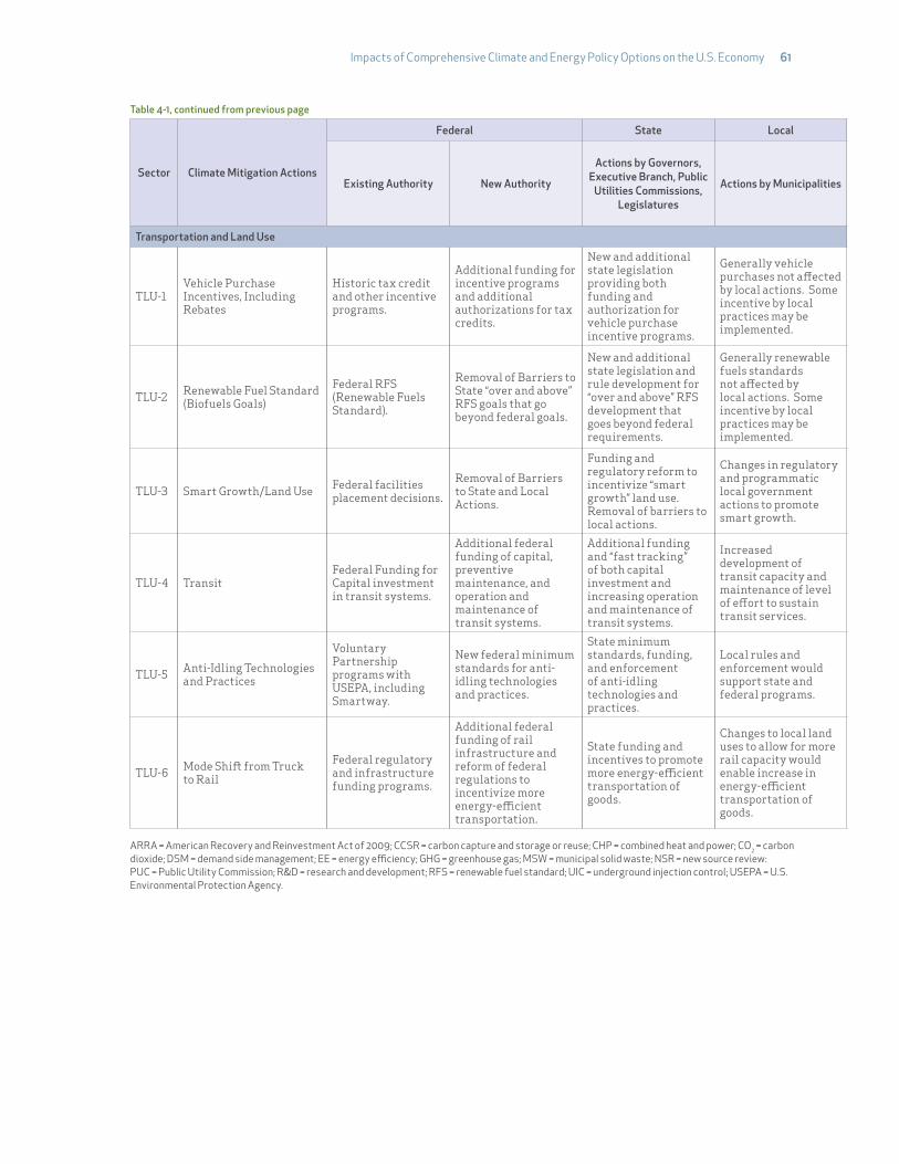
Impacts of Comprehensive Climate and Energy Policy Options on the U.S. Economy !61
Sector Climate Mitigation Actions
Federal State Local
Existing Authority New Authority
Actions by Governors, Executive Branch, Public
Utilities Commissions, Legislatures
Actions by Municipalities
Transportation and Land Use
TLU-1Vehicle Purchase Incentives, Including Rebates
Historic tax credit and other incentive programs.
Additional funding for incentive programs and additional authorizations for tax credits.
New and additional state legislation providing both funding and authorization for vehicle purchase incentive programs.
Generally vehicle purchases not a!ected by local actions. Some incentive by local practices may be implemented.
TLU-2 Renewable Fuel Standard (Biofuels Goals)
Federal RFS (Renewable Fuels Standard).
Removal of Barriers to State “over and above” RFS goals that go beyond federal goals.
New and additional state legislation and rule development for “over and above” RFS development that goes beyond federal requirements.
Generally renewable fuels standards not a!ected by local actions. Some incentive by local practices may be implemented.
TLU-3 Smart Growth/Land Use Federal facilities placement decisions.
Removal of Barriers to State and Local Actions.
Funding and regulatory reform to incentivize “smart growth” land use. Removal of barriers to local actions.
Changes in regulatory and programmatic local government actions to promote smart growth.
TLU-4 TransitFederal Funding for Capital investment in transit systems.
Additional federal funding of capital, preventive maintenance, and operation and maintenance of transit systems.
Additional funding and “fast tracking” of both capital investment and increasing operation and maintenance of transit systems.
Increased development of transit capacity and maintenance of level of e!ort to sustain transit services.
TLU-5 Anti-Idling Technologies and Practices
Voluntary Partnership programs with USEPA, including Smartway.
New federal minimum standards for anti-idling technologies and practices.
State minimum standards, funding, and enforcement of anti-idling technologies and practices.
Local rules and enforcement would support state and federal programs.
TLU-6 Mode Shi# from Truck to Rail
Federal regulatory and infrastructure funding programs.
Additional federal funding of rail infrastructure and reform of federal regulations to incentivize more energy-e$cient transportation.
State funding and incentives to promote more energy-e$cient transportation of goods.
Changes to local land uses to allow for more rail capacity would enable increase in energy-e$cient transportation of goods.
ARRA = American Recovery and Reinvestment Act of 2009; CCSR = carbon capture and storage or reuse; CHP = combined heat and power; CO2 = carbon dioxide; DSM = demand side management; EE = energy e%ciency; GHG = greenhouse gas; MSW = municipal solid waste; NSR = new source review: PUC = Public Utility Commission; R&D = research and development; RFS = renewable fuel standard; UIC = underground injection control; USEPA = U.S. Environmental Protection Agency.
Table 4-1, continued from previous page
62!Johns Hopkins University and Center for Climate Strategies
This study summarizes the analysis of the impacts of 23 major, sector-based GHG mitigation policy options on the U.S. economy in combination with U.S. Senate proposed cap and trade programs for the Electricity and Industrial sectors. We linked state of the art microeconomic analyses and macroeconometric model to perform this analysis. The data, assumptions, and methods used in this study are based on the results of formal agreements by over 1,500 stakeholders made through intensive, deliberative processes that used formal consensus building, fact finding, and analysis techniques. They further include scale-up of costs and savings estimates reported in the climate action plans of sixteen U.S. states to the national level.
Findings show potential national improvements from implementation of a top set of major sector-based policies and measures, to be implemented at all levels of government, of:
"» 2.5 million net new jobs in 2020 and a $159.6 billion expansion in GDP in 2020;
"» Over $5 billion net direct economic savings in 2020, at an average net savings of $1.57 per ton of GHG emissions avoided or removed;
"» Consumer energy price reductions of 0.56% for gasoline and oil; 0.60% for fuel oil and coal; 2.01% for electricity; and 0.87% for natural gas by 2020.
Assuming full and appropriately scaled implementation of all 23 actions in all U.S. states, the resulting GHG reductions would surpass national GHG targets proposed by President Obama and congressional legislation, and would reduce U.S. emissions to 27% below 1990 levels in 2020, equal to 4.46 billion metric tons of carbon dioxide equivalent (BMtCO2e) (see Figure 5-1).
The study also examined the e!ects of a stylized version of a cap-and-trade program as specified in the May, 2010 version of the Kerry-Lieberman climate bill. It was assumed that about 21% of cap-and-trade allowances from the Electricity and Industrial sectors will be auctioned in 2020, and that about 50% of the auction revenue will be returned back to low-income consumers and the remaining revenue will be used in Highway Trust Fund and deficit reduction.
If full and appropriately scaled implementation of all 23 actions in all U.S. states is coupled with the Senate proposed cap-and-trade program for the Electricity and Industrial sectors, with strong revenue recycling to low-income consumers, national improvements are expected to include:
"» 2.1 million net new jobs in 2020 and $116.9 billion expansion in GDP in 2020;
"» Over $5 billion net economic savings in 2020, at an average of $1.57 net savings per ton GHG emissions removed;
"» Consumer energy price decreases of 0.18% for gasoline, 1.74% for electricity; and 0.31% for natural gas by 2020;
"» $19.2 billion in new government revenues (prior to recycling to consumers and Highway Trust Fund).
%&'()*+ 2)4&
» Conclusions
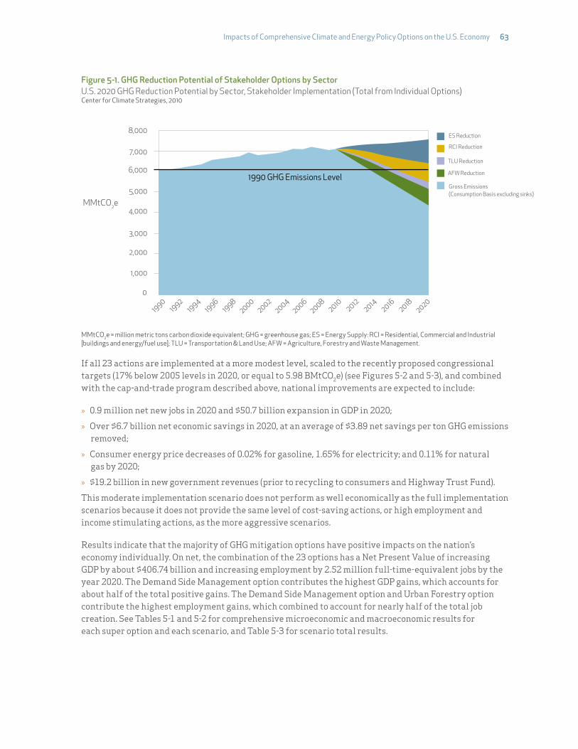
Impacts of Comprehensive Climate and Energy Policy Options on the U.S. Economy !63
Figure 5-1. GHG Reduction Potential of Stakeholder Options by Sector U.S. 2020 GHG Reduction Potential by Sector, Stakeholder Implementation (Total from Individual Options)Center for Climate Strategies, 2010
MMtCO2e
0
19901992
19941996
19982000
20022004
20062008
20102012
20142016
20182020
1,000
2,000
3,000
4,000
5,000
6,000
7,000
8,000
1990 GHG Emissions Level
ES Reduction
RCI Reduction
TLU Reduction
AFW Reduction
Gross Emissions(Consumption Basis excluding sinks)
MMtCO2e = million metric tons carbon dioxide equivalent; GHG = greenhouse gas; ES = Energy Supply: RCI = Residential, Commercial and Industrial [buildings and energy/fuel use]; TLU"="Transportation & Land Use; AFW = Agriculture, Forestry and Waste Management.
If all 23 actions are implemented at a more modest level, scaled to the recently proposed congressional targets (17% below 2005 levels in 2020, or equal to 5.98 BMtCO2e) (see Figures 5-2 and 5-3), and combined with the cap-and-trade program described above, national improvements are expected to include:
"» 0.9 million net new jobs in 2020 and $50.7 billion expansion in GDP in 2020;
"» Over $6.7 billion net economic savings in 2020, at an average of $3.89 net savings per ton GHG emissions removed;
"» Consumer energy price decreases of 0.02% for gasoline, 1.65% for electricity; and 0.11% for natural gas by 2020;
"» $19.2 billion in new government revenues (prior to recycling to consumers and Highway Trust Fund).
This moderate implementation scenario does not perform as well economically as the full implementation scenarios because it does not provide the same level of cost-saving actions, or high employment and income stimulating actions, as the more aggressive scenarios.
Results indicate that the majority of GHG mitigation options have positive impacts on the nation’s economy individually. On net, the combination of the 23 options has a Net Present Value of increasing GDP by about $406.74 billion and increasing employment by 2.52 million full-time-equivalent jobs by the year 2020. The Demand Side Management option contributes the highest GDP gains, which accounts for about half of the total positive gains. The Demand Side Management option and Urban Forestry option contribute the highest employment gains, which combined to account for nearly half of the total job creation. See Tables 5-1 and 5-2 for comprehensive microeconomic and macroeconomic results for each super option and each scenario, and Table 5-3 for scenario total results.

64!Johns Hopkins University and Center for Climate Strategies
Figure 5-2. GHG Reductions – Stakeholder and Congressional Target Scenarios U.S. 1990-2020 GHG Reduction Potential, Congressional Target and Stakeholder Target ScenariosCenter for Climate Strategies, 2010
MMtCO2e
0
19901992
19941996
19982000
20022004
20062008
20102012
20142016
20182020
1,000
2,000
3,000
4,000
5,000
6,000
7,000
8,000
9,000Baseline Emissions Stakeholder TargetCongressional Target
MMtCO2e = million metric tons carbon dioxide equivalent; GHG = greenhouse gas.Stakeholder Target = 27% below 1990 levels by 2020; Congressional Target = 17% below 2005 levels by 2020.
Figure 5-3. Stakeholder Policies Scaled to Achieve Congressional GHG Target U.S. 2020 GHG Reduction Potential by Sector, Congressional Implementation (Total from Individual Options)Center for Climate Strategies, 2010
MMtCO2e
0
19901992
19941996
19982000
20022004
20062008
20102012
20142016
20182020
1,000
2,000
3,000
4,000
5,000
6,000
7,000
8,000
1990 GHG Emissions Level
ES Reduction
RCI Reduction
TLU Reduction
AFW Reduction
Gross Emissions(Consumption Basis excluding sinks)
MMtCO2e = million metric tons carbon dioxide equivalent; GHG = greenhouse gas; ES = Energy Supply: RCI = Residential, Commercial and Industrial [buildings and energy/fuel use]; TLU"="Transportation & Land Use; AFW = Agriculture, Forestry and Waste Management.
Impacts of Comprehensive Climate and Energy Policy Options on the U.S. Economy !65
The economic gains result primarily from the ability of mitigation options to lower the cost of production. This stems primarily from their ability to improve energy e$ciency and thus lower production costs and higher consumer purchasing power. The results are also due to the stimulus of increased investment in plant and equipment.
Several tests were performed to determine the sensitivity of the results to major changes in key variables such as capital costs and avoided fuel costs. The sensitivity tests indicate that lower capital cost or higher value of avoided energy costs of the mitigation policy options would result in more favorable outcomes to the economy.
The estimates of economic benefits reported in this study represent a lower bound from a broader perspective. They do not include the avoidance of damage from the climate change that continued baseline GHG emissions would bring forth, the reduction in damage from the associated decrease in ordinary pollutants, the reduction in the use of natural resources, the reduction in tra$c congestion, etc.
Overall, the findings from this study suggest that implementing the various mitigation policy options recommended in the state climate change action plans at the federal level would generate net positive economic impacts to the nation’s economy.
Recommended actions by state climate change stakeholders included policies and measures in all sectors, at all levels of government (under a national framework), and a variety of specific matching policy instruments (including price and non price approaches) needed for achieving GHG targets, economic and energy benefits. For instance, policy tools for the 23 actions selectively include targeted funding support, tax incentives, price incentives, reform of codes and standards, technical assistance, information and education, reporting and disclosure, and voluntary or negotiated agreements.
Analysis also shows the importance of integrating local, state and federal actions, as well as policy instruments, to minimize costs and maximize co-benefits. For example:
"» 38% of total potential emissions reductions can be achieved through measures under shared federal and state jurisdiction;
"» 31%of potential emissions reductions can be achieved through measures primarily under state jurisdiction;
"» 31% of potential emissions reductions can be achieved through measures primarily under local or shared local/state jurisdiction.
The study underscores the strategic benefits of comprehensive approaches to managing GHG emissions, the need for a national framework to support a “balanced portfolio” of actions, and the importance of stakeholder involvement in policy development and management of the economy.
Key findings of this study include:"» Sector-based GHG reduction policies that are carefully selected and designed can result in net positive
outcomes for employment, income, and gross domestic product, as well as reducing energy prices.
"» Applying 23 major policies recommended by state-stakeholders for climate, energy, transportation, and resource actions in all 50 states, through combined federal, state and local approaches, would yield significant national economic benefits.
"» Most state stakeholder-recommended climate and energy actions will have net positive impacts to the economy and employment, but some, while substantially reducing GHGs and improving energy security, will have net negative impacts without additional policy support, such as revenue recycling to low income consumers and key industries.

66!Johns Hopkins University and Center for Climate Strategies
"» Comprehensive approaches that draw upon the best choices in all sectors, all levels of government, and all applicable policy instruments (including price and non price approaches) can a"ain GHG targets while minimizing costs and maximizing co-benefits (including energy and environmental security).
"» In the view of stakeholders, no single policy or tool can achieve the desired GHG reductions needed to meet GHG targets and simultaneously meet economic, energy and environmental objectives in a socially and politically acceptable manner; a combined approach is needed.
"» State Climate Action Plans have demonstrated that decisions on the specifics of policy design and implementation (i.e., stringency, coverage, timing), implementation tools, and other factors, can dramatically a!ect the economic and social performance of individual policies.
"» The two most significant barriers to full implementation of climate and energy polices are adequate investment and authority at the program level.
"» Federal preemption of these 23 policies where state and local programs are needed could impede some of the nations’ most cost-e!ective and job-creating actions.
"» Federal, state and local jurisdictions must be partners to capture the e$ciencies of comprehensive policy. The broadest jurisdictional reach rests with the states.
"» Locally and regionally derived policies can be translated to action in all 50 states, but require a national framework for full implementation.
"» If caps and taxes are combined with appropriate sector-based policies and measures, their cost will be lower and their co-benefits will be significantly higher than if they are implemented alone.
"» Auctions of allowances in key sectors will have negative impacts on economic performance if funds are not recycled e!ectively. However, reinvestment to targeted support for low-income consumers and key industries can significantly reverse these impacts.
"» Policy strategies applicable to the next decade must be combined with longer term policies to address future decades, and provide an important transition.

Impacts of Comprehensive Climate and Energy Policy Options on the U.S. Economy !67
Table 5-1. Impacts of 23 Stakeholder-Recommended, Sector-Based Climate and Energy Policy Options on the U.S. Economy – Fully Implemented Stakeholder Proposals Plus Cap-and-Trade and Revenue Recycling
Sector Climate Mitigation Actions
2020 Annual GHG Reduction (MMtCO2e)
Cost or Cost Savings per
Ton GHG Removed ($)
2020 Annual Cost or
Cost Savings
(million $)
2020 Net Employment
Impact (thousands)
2020 GDP Impact
(billion $)
Impact on GDP 2010–2020 NPV (billion $)
AFW–1 Crop Production Practices to Achieve GHG Benefits 65.01 –$15.69 –$1,020 87.7 $4.55 $17.50
AFW–2Livestock Manure – Anaerobic Digestion and Methane Utilization
19.25 $11.27 $217 –0.9 –$0.17 –$0.58
AFW–3 Forest Retention 39.21 $39.38 $1,544 71.2 $0.48 $3.45
AFW–4 Reforestation/A!orestation 178.77 $33.18 $5,932 –117.8 –$11.07 –$73.47
AFW–5 Urban Forestry 39.96 $15.35 $613 505.3 $5.44 $40.12
AFW–6 MSW Source Reduction 147.09 –$3.20 –$471 25.7 $2.53 $10.37
AFW–7 Enhanced Recycling of Municipal Solid Waste 249.27 $13.39 $3,339 114.4 $10.38 $51.61
AFW–8 Landfill Gas Management 48.38 $0.34 $17 94 $10.44 $26.47
Agriculture, Forestry, Waste Management (AFW) Totals 786.96 $12.92 $10,170 779.6 $22.58 $75.46
ES–1 Renewable Portfolio Std. 508.39 $17.84 $9,071 –58.6 –$5.35 –$35.52
ES–2 Nuclear 300.77 $26.98 $8,116 –73.3 –$6.85 –$8.14
ES–3 Carbon Capture Sequestration/Reuse 130.23 $32.92 $4,287 –35.4 –$4.47 –$16.57
ES–4 Coal Plant E$ciency Improvements and Repowering 151.05 $12.95 $1,956 1.1 $0.48 $0.86
Energy Supply (ES) Totals 1,090.45 $21.49 $23,430 –166.2 –$16.19 –$59.38
RCI–1 Demand Side Management Programs 424.80 –$40.71 –$17,293 886.2 $90.05 $305.05
RCI–2 High Performance Buildings (Private and Public) 193.88 –$24.99 –$4,845 183.3 $12.12 $40.14
RCI–3 Appliance standards 80.86 –$53.21 –$4,302 25.1 $0.05 –$0.43
RCI–4 Building Codes 161.08 –$22.86 –$3,682 181.1 $13.65 $49.05
RCI–5 Combined Heat and Power 136.37 –$13.18 –$1,798 –127.9 –$21.17 –$104.38
Residential, Commercial and Industrial (RCI) Totals 996.98 –$32.02 –$31,920 1,147.80 $94.70 $289.44
TLU–1 Vehicle Purchase Incentives, Including Rebates 103.07 –$66.37 –$6,841 179.5 $16.51 $39.64
TLU–2 Renewable Fuel Standard (Biofuels Goals) 92.34 $57.14 $5,277 –25.2 –$4.78 –$17.08
TLU–3 Smart Growth/Land Use 71.04 –$1.11 –$79 165.7 $6.15 $19.54
TLU–4 Transit 27.05 $16.72 $452 52.2 $1.18 $2.46
TLU–5 Anti–Idling Technologies and Practices 33.82 –$65.19 –$2,205 16.7 $1.92 $2.96
TLU–6 Mode Shi# - Truck to Rail 36.85 –$91.56 –$3,374 40.9 $6.69 $2.92
Transportation and Land Use (TLU) Totals 364.17 –$18.59 –$6,770 429.8 $27.68 $50.4423 Policy Totals (summation) 3,238.57 –$1.57 –$5,090 2,191 $128.77 $355.97Stakeholder Recommendations Scenario Results (simultaneous) 3,238.57 –$1.57 –$5,090 2,524 $159.60 $406.74
Stakeholder Recommendations w/Cap & Trade + Revenue Recycling 3,238.57 –$1.57 –$5,090 2,132 $116.90 n.a.
GDP = gross domestic product; GHG = greenhouse gas; MMtCO2e = million metric tons carbon dioxide equivalent; MSW = municipal solid waste; NPV = net present value. Note: The 23 Policy Totals are a simple summation of each policy’s estimated results; interactions and double counting between policies have been accounted for in indi-vidual policy results; the Stakeholder Scenario simultaneous results of the REMI analysis take into account the interactive economic e#ects of policies.

68!Johns Hopkins University and Center for Climate Strategies
Table 5-2. Impacts of 23 Stakeholder-Recommended, Sector-Based Climate and Energy Policy Options on the U.S. Economy – U.S. Congressional Target Plus Cap-and-Trade and Revenue Recycling
Sector Climate Mitigation Actions
2020 Annual GHG Reduction Potential
(MMtCO2e)
Cost or Cost Savings per
Ton GHG Removed ($)
2020 Annual Cost or Cost Savings
(million $)
2020 Net Employment
Impact (thousands)
2020 GDP Impact
(billion $)
Impact on GDP 2010-2020 NPV (billion $)
AFW-1 Crop Production Practices to Achieve GHG Benefits 17.30 –$15.69 –$271 23.34 $1.21 $4.66
AFW-2Livestock Manure - Anaerobic Digestion and Methane Utilization
5.12 $11.27 $58 –0.24 –$0.05 –$0.15
AFW-3 Forest Retention 10.43 $39.38 $411 18.95 $0.13 $0.91
AFW-4 Reforestation/A!orestation 47.57 $33.18 $1,578 –31.35 –$2.95 –$19.55
AFW-5 Urban Forestry 10.63 $15.35 $163 134.46 $1.45 $10.68
AFW-6 MSW Source Reduction 39.14 –$3.20 –$125 6.84 $0.68 $2.76
AFW-7 Enhanced Recycling of Municipal Solid Waste 66.33 $13.39 $888 30.44 $2.77 $13.73
AFW-8 Landfill Gas Management 12.87 $0.34 $4 25.01 $2.78 $7.04
Agriculture, Forestry, Waste Management (AFW) Totals 209.40 $12.92 $2,706 207.45 $6.01 $20.08
ES-1 Renewable Portfolio Standard 312.93 $17.84 $5,584 –36.07 –$3.29 –$21.86
ES-2 Nuclear 185.13 $26.98 $4,995 –45.12 –$4.22 –$5.01
ES-3 Carbon Capture Sequestration/Reuse 80.16 $32.92 $2,639 –21.79 –$2.74 –$10.20
ES-4Coal Plant E$ciency Improvements and Repowering
92.98 $12.95 $1,204 0.68 $0.30 $0.52
Energy Supply (ES) Totals 671.20 $21.49 $14,422 –102.30 –$9.97 –$36.54
RCI-1 Demand Side Management Programs 261.48 –$40.71 –$10,644 545.48 $55.43 $187.76
RCI-2 High Performance Bldgs. (Public and Private) 119.34 –$24.99 –$2,982 112.83 $7.46 $24.71
RCI-3 Appliance Standards 49.77 –$53.21 –$2,648 15.45 $0.02 –$0.26
RCI-4 Building Codes 99.15 –$22.86 –$2,266 111.47 $8.40 $30.19
RCI-5 Combined Heat and Power 83.94 –$13.18 –$1,107 –78.73 –$13.03 –$64.25
Residential, Commercial and Industrial (RCI) Totals 613.67 –$32.02 –$19,647 706.50 $58.28 $178.16
TLU-1Vehicle Purchase Incentives, Including Rebates
63.44 –$66.37 –$4,211 110.49 $10.17 $24.40
TLU-2 Renewable Fuel Std. (Biofuels Goals) 56.84 $57.14 $3,248 –15.51 -$2.93 -$10.51
TLU-3 Smart Growth/Land Use 43.73 –$1.11 –$49 101.99 $3.79 $12.03
TLU-4 Transit 16.65 $16.72 $278 32.13 $0.72 $1.51
TLU-5 Anti-Idling Technologies and Practices 20.82 -$65.19 –$1,357 10.28 $1.19 $1.82
TLU-6 Mode Shi# from Truck to Rail 22.68 –$91.56 –$2,077 25.17 $4.12 $1.79
Transportation and Land Use (TLU) Totals 224.16 –$18.59 –$4,168 264.55 $17.04 $31.05

Impacts of Comprehensive Climate and Energy Policy Options on the U.S. Economy !69
Sector Climate Mitigation Actions
2020 Annual GHG Reduction Potential
(MMtCO2e)
Cost or Cost Savings per
Ton GHG Removed ($)
2020 Annual Cost or Cost Savings
(million $)
2020 Net Employment
Impact (thousands)
2020 GDP Impact
(billion $)
Impact on GDP 2010-2020 NPV (billion $)
23 Policy Totals (summation) 1,718.43 –$3.89 –$6,687 1,076 $71.36 $192.74
Congressional Target Results w/o C&T + Revenue Recycling 1,718.43 –$3.89 –$6,687 1,147 $76.91 $195.50
Congressional Target Results w/Cap & Trade + Revenue Recycling 1,718.43 –$3.89 –$6,687 922 $50.73 n.a.
GHG = greenhouse gas; MMtCO2e = million metric tons carbon dioxide equivalent; GDP = gross domestic product: MSW = municipal solid waste; NPV = net present value. Negative numbers indicate cost savings.Note: The 23 Policy Totals are a simple summation of each policy’s estimated results; interactions and double counting between policies have been ac-counted for in individual policy results; the Stakeholder Scenario simultaneous results of the REMI analysis take into account the interactive economice#ects of policies.
Table 5-3. Summary of GHG Reductions, Direct Costs/Savings, and Macroeconomic Results
Scenario2020
GHG Reductions (BMtCO2e)a
2020 Direct Net Cost
(billion $)b
2020 Net New Jobs
(million $)
2020 GDP Expansion (billion $)
Total 2020 New Gov’t Revenue
(billion $)c
23 Stakeholder Policy Recommendations at Full Implementation
3.2 –$5.1 2.52 $159.6 n.a.
23 Stakeholder Policy Recommendations, Full Implementation, plus Cap-and-Trade & Revenue Recycling
3.2 –$5.1 2.13 $116.9 $19.2
23 Stakeholder Policy Recommendations at Congressional Economy-Wide Target levels, plus Cap-and-Trade & Revenue Recycling
1.7 –$6.7 0.92 $50.7 $19.2
a Reductions from estimated business-as-usual 2020 baseline emissions of 7.7 BMtCO2e; BMtCO2e = billion metric tons of carbon dioxide equivalent.b Negative numbers indicate net savings; positive numbers indicate net costs.c Direct revenues from Cap-and-Trade program allowance auction, not including use or distribution of revenues.
Table 5-2, continued from previous page

70!Johns Hopkins University and Center for Climate Strategies
In addition to these references and data sources used directly in the study, each of the individual state plans that served as the basis for this report relied on a significant number of additional studies and information sources. For listings of these studies and sources, see the appendixes of the individual state reports available on the CCS Web site at www.climatestrategies.us.
ReferencesAmerican Association of State Highway and Transportation O$cials. Transportation Invest in America Freight-Rail Bo#om Line Report. Available at: www.freight.transportation.org/doc/FreightRailReport.pdf.
Center for Climate Strategies (CCS). 2009. Southern Regional Economic Assessment of Climate Policy Options and Review of Economic Studies of Climate Policy. Available at: www.climatestrategies.us/template.cfm?FrontID=6081.
Coase, R. 1960. “The Problem of Social Cost,” Journal of Law and Economics 3(1): 1-44.
Doniger, David. May 2010. American Power Act: “First Read” of the Kerry-Lieberman Climate and Energy Legislation, Natural Resources Defense Council.
Ellerman, A.D. 2008. “The EU Emission Trading Scheme: Prototype of a Global System?” Discussion Paper 08-02, The Harvard Project on International Climate Agreements.
Ellerman, A.D., Joskow, P.L., Schmalensee, R., Montero, J., and Bailey, E.M. 2000. Markets for Clean Air: The U.S. Acid Rain Program. Cambridge, UK: Cambridge University Press
Granade, H.C., Creyts, J., Derkach, A., Farese, P, Nyquist, S., and Ostrowski, K. 2009. Unlocking Energy E$ciency in the U.S. Economy. McKinsey Global Energy and Materials.
Kerry, John, and Lieberman, Joseph. 2010. American Power Act. U.S. Senate. www.lieberman.senate.gov/assets/pdf/APA_full.pdf.
Laitner, J.A. “Skip.” 2009. Climate Change Policy as an Economic Redevelopment Opportunity: The Role of Productive Investments in Mitigating Greenhouse Gas Emissions. ACEEE Report E098. Washington, DC, American Council for an Energy-E$cient Economy.
McKinstry, R.B., Peterson, T.D., Rose, A., and Wei, D. 2009. “The New Climate World: Achieving Economic E$ciency in a Federal System for GHG Regulation through State Planning,” North Carolina Journal of International Law and Commercial Regulation 34(3): 767-850.
Miller, S., Wei, D., and Rose, A. 2010. The Economic Impact of the Michigan Climate Change Action Plan on the State’s Economy. Report to the Michigan Department of Environmental Quality, The Center for Climate Strategies, Washington DC.
Montgomery, W. D., Plewes, J., Smith, A.E., and Tuladhar, S.D. 2007. Economic Analysis of Florida’s Executive Order 07-127. Charles Rivers Associates. Prepared for Florida Chamber of Commerce and US Chamber of Commerce.
%&'()*+ %)5
» References and Data Sources
Impacts of Comprehensive Climate and Energy Policy Options on the U.S. Economy !71
National Commission on Energy Policy. 2004. Ending the Energy Stalemate: A Bipartisan Strategy to Meet America’s Energy Challenge, www.energycommission.org.
Partridge, M.D., and Richman, D.S. 1998. “Regional Computable General Equilibrium Modeling: A Survey and Critical Appraisal,” International Regional Science Review 21(3), 205-248.
Regional Economic Models, Inc. 2009. REMI PI+ Model Document. Available at: www.remi.com.
Roland-Holst, D., and Karhl, F. The Florida Economy and a Federal Carbon Cap: A Quantitative Analysis. 2009. Department of Agricultural and Resources Economics Working Paper, University of California, Berkeley.
Rose, A. 2009. The Economics of Climate Change Policy: International, National and Regional Strategies, Cheltenham, UK: Edward Elgar Publishing Company.
Rose, A., and Miernyk, W. 1989. “Input-Output Analysis: The First Fi#y Years,” Economic Systems Research 1(2): 229-271.
Rose, A., and G. Oladosu. 2002. “Greenhouse Gas Reduction in the U.S.: Identifying Winners and Losers in an Expanded Permit Trading System,” Energy Journal 23(1): 1-18.
Rose, A., and Wei, D. 2009a. The Economic Impact of the Florida Energy and Climate Change Action Plan on the State’s Economy. Report to the O$ce of the Governor of the State of Florida, The Center for Climate Strategies, Washington DC.
Rose, A., and Wei, D. 2009b. “Macroeconomic Assessment,” Chapter 11 in Pennsylvania Climate Action Plan. www.depweb.state.pa.us/energy/cwp/view.asp?q=539829.
Rose, A., Wei, D., Wennberg, J., and Peterson, T. 2009. “Climate Change Policy Formation in Michigan: The Case for Integrated Regional Policies,” International Regional Science Review 32(4): 445-465.
Ross, M.T., Murray, B.C., Beach, R.H., Depro, B.M., and RTI International. 2008. State-level Economic Impacts of a National Climate Change Policy. Pew Center on Global Climate Change. White Paper.
Tietenberg, T. 1985. Emissions Trading: An Exercise in Reforming Pollution Policy. Washington, DC: Resources for the Future).
Tietenberg, T. 2007. “Tradable Permits in Principle and Practice,” in J. Freemand and C. Kolstad (eds.), Moving to Markets: Lessons from Twenty Years of Experience. New York: Oxford University Press.
Transportation Research Board. 2004. “Long-Haul Tractor Idling Alternative.” Table 1. See epa.gov/smartway/documents/dewi"-study.pdf.
Treyz, G. 1993. Regional Economic Modeling: A Systematic Approach to Economic Forecasting and Policy Analysis. Boston: Kluwer.
U.S. Census Bureau. 2002. 2002 Economic Census: Vehicle Inventory and Use Survey. Available at: www.census.gov/prod/ec02/ec02tv-us.pdf.
U.S. Environmental Protection Agency (EPA). 2009. The E!ects of H.R.2454 on International Competitiveness and Emission Leakage in Energy-Intensive Trade-Exposed Industries. An interagency Report Responding to a Request from Senators Bayh, Specter, Stabenow, McCaskill, and Brown. Available at: www.epa.gov/climatechange/economics/economicanalyses.html#interagency.
Ward, J. VISION 2008 User’s Guide. Washington, DC: U.S. Department of Energy. October, 2008.
72!Johns Hopkins University and Center for Climate Strategies
Data SourcesAmerican Council for an Energy-E$cient Economy. 2008. The 2008 State Energy E$ciency Scorecard. www.aceee.org/pubs/e086_es.pdf.
Central Intelligence Agency. 2009. The World Factbook. h"ps://www.cia.gov/library/publications/the-world-factbook/rankorder/2004rank.html.
ONSITE SYCOM Energy Corporation. 2000. The Market and Technical Potential for Combined Heat and Power in the Commercial/Institutional Sector, pp.57–58. www.eere.energy.gov/de/pdfs/chp_comm_market_potential.pdf.
U.S. Bureau of the Census. 2002. 2002 Economic Census: Vehicle Inventory and Use Survey. Available at: www.census.gov/prod/ec02/ec02tv–us.pdf.
U.S. Bureau of the Census, Population Division. 2004. State Interim Population Projections by Age and Sex: 2004–2030. www.census.gov/population/www/projections/projectionsagesex.html.
U.S. Bureau of the Census. 2009. Heating- and Cooling-Degree Days. www.census.gov/compendia/statab/tables/09s0379.xls.
U.S. Bureau of Economic Analysis. 2009. Gross Domestic Product by State. www.bea.gov/regional/gsp.
U.S. Bureau of Economic Analysis and Bureau of the Census. 2008. State Personal Income 2008. www.bea.gov/newsreleases/regional/spi/spi_newsrelease.htm.
U.S. Department of Energy, Energy Information Administration. 2008. State Energy Data System. www.eia.doe.gov/emeu/states/hf.jsp?incfile=sep_sum/plain_html/sum.
U.S. Department of Energy, Energy Information Administration. 2009. Electric Power Annual 2007. www.eia.doe.gov/cneaf/electricity/epa/epa_sprdshts.html.
U.S. Department of Energy, Energy Information Administration. 2009. State Electric Profile. www.eia.doe.gov/cneaf/electricity/st_profiles/e_profiles_sum.html.

About the Governmental Studies Programs at Johns Hopkins UniversityThe Johns Hopkins MA in Government o!ers concentrations in security studies, legal studies, and political communication. The courses are designed to give students comprehensive knowledge of governmental institutions, their political development, and how they interact in the policy making process. With this knowledge the students are be"er equipped to examine governmental and social institutions, assess prospects for reform, e!ect change, and become tomorrow’s leaders.
Students may also pursue the MA in Global Security Studies which examines global security in the context of the 21st century. Students take courses which focus on three key sectors of security: military, economic, environmental and energy. The Master of Arts in Global Security Studies prepares students to lead the e!orts to meet challenges within each of these sectors and to help ensure a more secure future for the nation and globe.
Find out more atgovernment.jhu.edu
global-security.jhu.edu

1717 Massachuse!s Avenue NW Suite 104 Washington, DC 20036
advanced.jhu.edu
FPO FSC Logo
FPO Soy Ink Logo
GOV1031
» energypolicyreport.jhu.edu