3

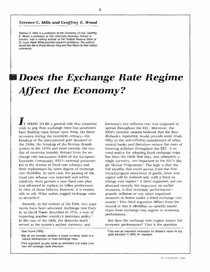
Terence C. Mills and Geoffrey F. Wood

Terence C. Mills is a professor at the University of Hull. GeoffreyE. Wood, a professor at City University Business School inLondon, was a visiting scholar at the Federal Reserve Bank ofSt Louis. Kevin White provided research assistanca The authorswould also like to thank Mervyn King and Paul Mizon for their helpfulcomments.

U Does the Exchange Rate RegimeAffect the Economy?

T SEEMS TO BE a general rule that countrieswish to peg their exchange rates but sometimeshave floating rates thrust upon them. On threeoccasions during the twentieth century—thebreakup of the international gold standald inthe l930s, the breakup of the Bretton Woodssystem in the 1970s and most recently the exo-dus of countries (notably Britain) from the ex-change rate mechanism (ERM) of the EuropeanEconomic Community (EEC)—external pi-essuresled to the demise of fixed rate schemes andtheir replacement by some degree of exchangerate flexibility. In each case, the passing of thefixed t-ate scheme was mourned and withinrelatively short periods a new fixed rate planwas advanced to replace its fallen predecessor.In view of these failures, however, it is reason-able to ask: What makes pegged exchange ratesso attractive?

Recently, in the context of the ERM, two argu-ments have been advanced. Exchange rate fixityis, as David flume described in 1752, a way ofimporting another country’s monetary policy.iIn the case of the ERM, the deutsche markserved as the system’s anchor currency, and

1See Flume (1970).2We do not consider whether a single currency really is anatural development of fixed exchange rates.

~Thisargument usually takes as axiomatic that trade crea-tion will outweigh trade diversion.

Germany’s low inflation i-ate was supposed tospread throughout the EEC. Moreover, theERM’s member nations believed that the Bun-desbank’s reputation would provide some credi-bility to the anti-inflation commitment of othercentral banks and therefore reduce the costs oflowering inflation throughout the EEC. A se-cond motive for adopting fixed exchange rateshas been the claim that they, and ultimately asingle currency, are important to the EEC’s Sin-gle Market Progt-amme.2 ‘I’he logic is that thefull benefits that could accrue fiom the freeintra-European movement of goods, labor andcapital will be realized only with a fixed ex-change rate regime.~A third argument, not em-phasized recently but important on earlieroccasions, is that economic perfot-mance-----growth, inflation or any other importantmeasure—is better under a fixed exchange ratesystem.4 This third argument differs from thesecond in that it identifies no specific causalchain ft’om exchange rate regime to economicperformance.

But does the exchange rate regime matter foreconomic performance? That is the question

4lhis was an important motivation for Britain’s return to thegold standard in 1925, for example.

4

addressed in this paper. We examine empiricallythe relationship between the exchange mate re-gime and a number of key macroeconomic vati-ables to see whether any systematic relationshipexists between the behavior of these variablesand the exchange rate regime. We have chosento investigate this question for the United King-dom because data over long periods are ayaila-ble for the variables we ivish to examine andbecause the United Kingdom experienced awide variety of exchange rate regimes over theperiod covered by these data.

TRADE -AND THE EXCHANGERATE REGIME

The claim that exchange rate flexibility ham-pers international trade in goods and in capitaland thus depresses welfare amid perhaps growthis based on the existence of uncertainty.

It is argued that removing the possibility ofexchange rate change will remove an importantnontarif F barrier, because the possibility of ex-change rate changes will deter some tradersand investors altogether, whereas others willhave to pay a substantial cost to fix the domes-tic value of their foreign currency receipts.Floating exchange rates, in other words, are be-lieved to impose additional volatility, and hencecosts, on international markets. If this is cor-rect, a case for pegged exchange rates exists,and the case is particularly strong fot anygroup of countries (such as the EEC) that wantsto encourage mutual international trade and in-vestment.

‘The proposition seems unexceptional, and fora number of years studies supported the propo-sition. For example, Cushman (1983) and de-Grauwe and deBellefroid (1937), which arerepresentative of the early literature, found thatfloating rates did impede trade. But as timepassed, an increasing number’ of studies sup-ported it.i

By the early I 990s, not only had evidenceshifted to support the notion that floating ex-change rates do not impede trade, but Feldstein(1992) even went so far as to suggest that float-

ing rates are more favorable to trade than arefixed rates.t Attention is thus directed to otherreasons for favoring pegged exchange tates.

‘rhere are two rather distinct types of effectsof exchange rate fixing. ‘I’he first arises becauseif a fixed exchange rate is in place, it is unlikelyto stay fixed without policy actions. These cantake several form& Most common are foreignexchange intervention and short-term interestrate manipulation. Accurate figures on officialintervention or the stock of foreign exchangereserves are not always availabla Interest ratefigures, however, are ayailable, and severalauthors have found that unpredictable interestrate variability increased after exchange ratesare pegged.~These actions in turn make moneygrowth more volatile, and this can have impor-tant consequences for the economy. It may cre-ate additional uncertainty about the futurehehayior of the price level and thus about realtates of return, which would affect investment.If future prices were uncertain, wage bargain-ing would he more complex because it wouldbe harder to judge the future purchasing powerof an agreed money wage. This uncertaintywould also affect nominal variables. Risk-averseinvestors would be more reluctant to buygovernment bonds because they would he un-certain what the coupons would be worth andwhat the capital would be worth at maturity.This would raise nominal interest rates, the costof debt service and thus the taxes necessary toservice the debt. All these factors could have anadvem’se effect on long-term growth, depressingits trend.

In summary, the choice of exchange rate re-gime could affect the long-run behavior of theeconomy, influencing trends or cycles in impor-tant macroeconomic variables.

If the choice of exchange rate regime does nothave these long-run consequences, then interms of macroeconomic effects, all that thechoice of exchange rate regime does is shift thedistribution of short-run fluctuations from onemarket to another. This is the second type ofeffect noted above.

‘The question we examine is whether any as-

tExamples of these studies are Gotur (1985); the IMF’s(1984) extension of Cushman (1983) to cover the bilateraltrade of the seven largest industrial countries; Bryant(1987), Bailey, Tavlas and Ulan (1986 and 1987), Bailey andTavlas (1988) and Ascheim, Bailey and Tavlas (1987).

tHaberler (1986) suggested the same thing some yearsearlier.

7See Batchelor and Wood (1982), Wood (1983) and Belongia(1988). Wood and Belongia’s research was conducted inthe context of the ERM. In Wood (1983) there was an ex-ception to this—Erie (South Ireland) after it joined theERM. Unpredictable interest rate variability fell in thatcountry, although it increased in every other ERM membercountry.

sociation exists between the exchange rate re-gime and the trend or cyclical behavior of somekey macroeconomic variables—in other words,whether there is any evidence for the first typeof effect. If no such association exists, then theonly macroeconomic consequence of the choiceof exchange rate regime is the change in thedistribution of short-term volatility between theforeign exchange market and the short-termmoney markets. If, in contrast, such an associa-tion exists, then the choice of exchange rate re-gime may be a macroeconomic policy decisionof considerable impot-tance for national well-heing.8

It is now appropriate to present the data weuse for exploring this question. We then exa-mine the properties of those data in light of thepreceding discussion.

THE STOCHASTIC PROPERTIESOF U.K. MACROECONOMIC SERIESACROSS EXCHANGE RATEREGIMES

In this section we consider the stochasticproperties of five major U.K. macroeconomicseries since the mid-nineteenth century. The ex-change rate regimes since then have encom-passed every possible type except the crawlingpeg. Until 1914, the United Kingdom was on thegold standard. That was suspended (that is, theUnited Kingdom left the standard but with thedeclared intention of returning) at the outbreakof World War I in 1914. After the war, theUnited Kingdom implemented a deliberate, dis-cussed and announced policy of a return to thegold standard at the prewar parity. Monetat-ypolicy and foreign exchange intervention wereused to this end, and the policy succeeded in1925. The United Kingdom left the gold stan-dard in 1931, however, and the exchange ratefloated with varying degrees of intervention un-til the outbreak of World Wat 11 in 1939.~Therate was then pegged to the U.S. dollat. After

5

the wat-, the United Kingdom joined the BrettonWoods system. Several sterling devaluations oc-curred under Bretton Woods, but sterling didnot finally float until 1972. Again, there werevatying degrees of intervention under this re-gime of dirty floating, hut the United Kingdomdid not formally peg sterling until it joined theERM in 1990 after shadowing the deutschemark in 1988 and 1989. The United Kingdomsubsequently left the ERM in 1992 to float oncemore. The series we examine across these vari-ous regimes are output, prices, money, andshort- and long-term interest rates.

Our particular interest, and the focus of theempirical work that follows, is the trend andthe cycle in output and prices primarily, hutalso in money and interest rates. We look to seehow these var-iahles have behaved over- ourclose to a century-and-a-quarter- of data, seekingchanges in trend and changes in cyclical pat-tern. When these are identified, we examinewhether any of these changes are associatedwith exchange rate regime changes and, if so,considei why this might he.

Output

Annual output in the United Kingdom (incas-ured in logarithms) over’ the period 1855-1990is shown in figure 1. Detailed econometric ana-lyses of this series in Mills (1991) and Mills andWood (1993) show that it can he represented asthe sum of a segmented linear trend, withbreaks at 1918 and 1921 and a stationary, au-toregressive, cyclical component.1°Thus theseresults indicate that if output can he decom-posed as = + ri, then the trend function t~,is

(1) ~, = a + Bt + A,D,, + A7])2,,

where D~=(t—T)if t>T,. and zero otherwise.The identified breakpoints are at = 64 andT

2=67, which coincide with 1918 and 1921. The

cyclical component, n,, on the other hand, isfound to be adequately modeled as an AR(2)

°Itis, of course, possible that the exchange rate regime is aproduct of the behavior of the economy; it need not be anexogenous choice.

tFor a review and evaluation of explanations that have beenadvanced to explain the United Kingdom’s abandonment ofthe gold standard, see Capie, Mills and Wood (1986a).

‘tTesting for stationarity has no direct economic significance.Rather, it lets us separate the cycle from the trend. Thenotion is that the trend and the cycle are economically

separate. The cycle comprises fluctuations about a horizon-tal average; growth is all in the trend- This separation isconsistent with most views of the cycle, but it should benoted that some scholars see the cycle as an integral partof the growth process- For an example, see Schumpeter(1950).

6

Figure 1Annual U.K. Output (1855-1990)Logarithms

6,50

6.00

5.50

5.00

4.50

4.00

3.50

process, leading to the fitted model (standarderrors shown in parentheses),

(2) Y, = 3.474 + 0.0196t —

(0.026) (0.0007J

0.1170Th + ri

(0.0 101)

0.1137]),, +

(0.0103)

= 1.099n, — 0.346rr, -, + a,(0.083) (0.083)

‘rhis model has some simple properties. Trendgrowth is 1.96 percent per year until 1919 and2.29 percent per year from 1922 on, with thelevel of trend output falling 28.3 percent in theintervening three years. The component n, im-plies that output exhibits stationary cyclical fluc-tuations around the trend growth path, withcycles averaging 8.1 year-s. The residual stan-dard error of the equation is 2.33 percent.

The trend component is shown superimposed

on the output series in figure 1, and we thusconclude that, apart from the three years im-mediately after World War I, during which theseries fell dramatically, the stochastic processgenerating output has remained remarkably sta-ble. Output is a trend stationary process, ir-respective of the exchange rate regime in force.

Prices

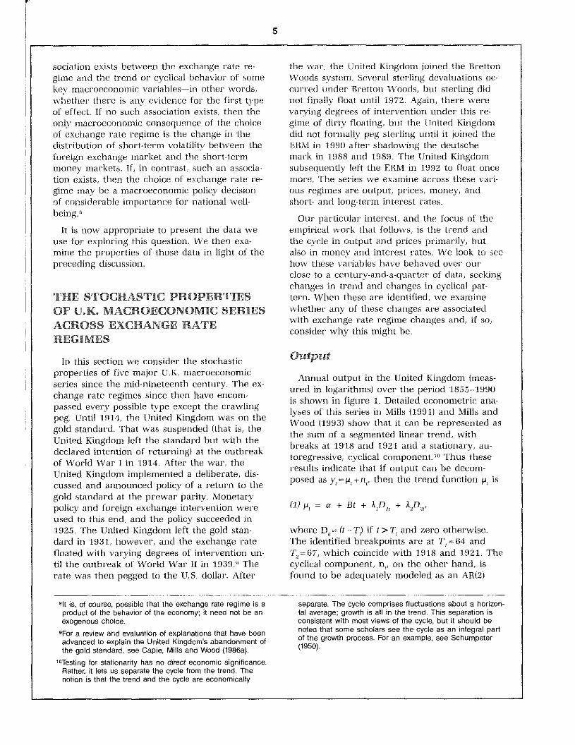
Figures 2 and 3 present plots of the (logarith-mic) U.K. price level annually from 1870 to1990 and monthly froni January 1922 to May1992, respectively, excluding the war yearsfrom 1940 to 1945. Unit root tests, calculatedover various sample periods, provide little or noevidence against the hypothesis that prices aredifference stationary, that is, 1(1).’’ Thepost-1973 era may differ and is discussed later.

Tivo aspects of price behavior are worth fur-

1860 70 80 90 1900 10 20 30 40 50 60 70 80 1990

“Details of these tests and similar tests for the other seriesinvestigated are reported in Mills and Wood (1993).

7

Figure 2Annual U.K. Price Level (1 870-1 939)

Logarithms

Annual UK. Price Level (1 946-1 990)

Logarithms

8.5-

8.0—

7.5—

7.0—

6.5—

6.0—

5.5—

5.0— I I I I I I I I I I I I I I I I I I I I I I

19464850525456586062646668707274767880828486881990

1870 75 80 85 90 95 1900 5 10 15 20 25 30 1935

8

Figure 3U.K. Price Level (1 922-1 939)

Logarithms

3

1922 23 24 25 26

U.K. Price Level (1 946-1 992)

27 28 29 30 31 32 33 34 35 36 37 381939

Logarithms

6.

6

5.

5.25

4

4.25

3.

3..194648 5052545658 6062 646668 7072 747678 8082 848688 901992

9

ther investigation. The first is the behavior ofthe price level before the United Kingdom aban-doned the gold standard in 1931. Mills (1990)analyzes the long gold standard period from1729 to 1931 and obtains an estimate of the lar-gest autoregressive root of 0.93, identical to thatobtained for the shorter sample beginning in1870. The corresponding unit root test, though,rejects the unit root null hypothesis at the 5percent significance level, and the processfound to generate the price level (an autoregres-sion of order two) yields cycles of around 50years, close to the long swings thought to havecharacterized prices during this period.”

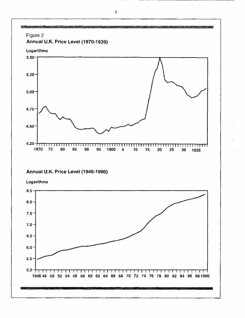
The second aspect concerns the post-1946 be-havior of prices. Figures 2 and 3 show the ser-ies to have undergone slope changes around1973 and 1983; possible explanations for theseare discussed in the next paragraph and in theInterpretation and Conclusions section. Statisti-cally, this behavior is typical of an 1(2) process,and repeating the unit root tests for the (log-arithmic) price changes, that is, for inflation,yields some evidence that postwar prices can bemodeled as an 1(2) process (evidence that infla-tion is nonstationary), particularly for the post-Bretton Woods era beginning in 1973.

The results are therefore suggestive of theU.K. price level undergoing two shifts in itsgenerating process. The first might be associat-ed with the abandonment of the gold standard,shifting the series from 1(0) to an 1(1) process.(From figure 3 it is in fact clear that prices didnot start a secular increase until mid-1933, sometwo years after the move from the gold stan-dard.)” A stable price level is certainly in accor-dance with what would be expected under thegold standard (or, in principle, any commoditystandard). There were fluctuations in the supplyof gold, but in countries such as the UnitedKingdom, which had developed and stable bank-ing systems, these fluctuations had only modestprice level effects. The system was to some ex-tent self-stabilizing. If prices were falling (thevalue of money rising) because the supply ofgold was falling short of demand, them-c was anincentive to produce more gold. And if priceswere rising (the value of money falling), then asthe costs of gold production rose relative towhat the monetary authorities would pay for

gold, the incentive to produce gold woulddiminish.” The second shift is around 1973 andcould be associated with both the move to float-ing exchange rates and the first oil price shock.

Money

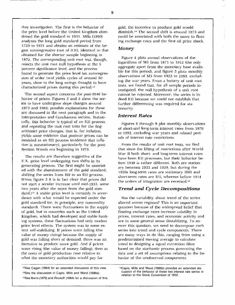
Figure 4 plots annual observations of thelogarithms of M3 from 1871 to 1912 (the onlyaggregate apart from the monetary base availa-ble for this period), and figure 5 plots monthlyobservations of M3 from 1922 to 1989, exclud-ing the war years. From a battery of unit roottests, we found that, for all sample periods in-vestigated, the null hypothesis of a unit rootcannot be rejected. Moreover, the series is in-deed 1(1) because we could not establish thatfurther differencing was required for sta-tionarity.

Interest Rates

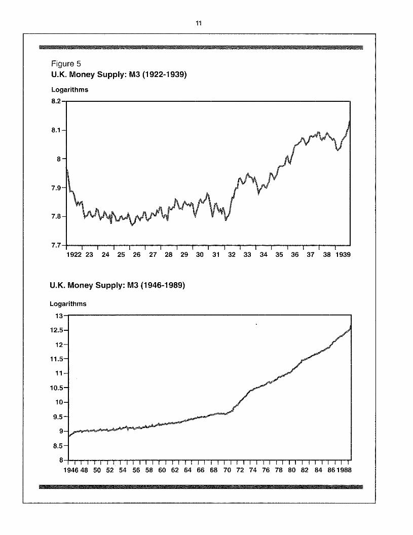
Figures 6 through 8 plot monthly observationsof short-and long-term interest rates from 1870to 1992, excluding war years and related peri-ods of interest rate restrictions.

From the results of unit root tests, we findthat since the lifting of restrictions after WorldWar II both short- and long-term interest rateshave been 1(1) processes, but their behavior be-fore 1939 is rather different. Both are station-ary between 1932 and 1939, but during the1920s long-term rates are stationary (1(0)) andshort-term rates are 1(1), whereas before 1914the orders of integration are reversed.”

Trend and Cycle Decompositions

Has the variability about trend of the seriesaltered across regimes? This is an importantquestion because of the widespread belief thatfloating exchange rates increase volatility inprices, interest rates, and economic activity andare in some general sense destablizing. To an-swer this question, we need to decompose eachseries into trend and cycle components. Thereare many ways to do this, ranging from using apredetermined moving average to calculatetrend to designing a signal extraction filterbased on the stochastic process generating thedata and a set of assumptions relating to the be-havior of the unobserved components.

ltSee Cagan (1984) for an extended discussion of this view,

ltSee the discussion in Capie, Mills and Wood (1986a).

‘4See Barro (1979) and Rockoff (1984) for a discussion of this.

‘tCapie, Mills and Wood (1986b) provides an extended dis-cussion of the behavior of these two interest rate series inrelation to the Stock Conversion of 1932.

10

Figure 4Annual U. K. Money Supply: M3 (1871-1912)

Logarithms

13.9

13.8—

13.7—

13.6—

13.5—

13.4—

13.3—

13.2—

13.1— —

1870

For output, equation (1) provides the appropri-ate decomposition. Table 1 thus reports thestandamd deviations of the cyclical component n,for a variety of sample periods. the sampleperiods shown were chosen by two quite dis-tinct criteria—output trend change and ex-change rate regime alteration. The 1922 breakwas used because after the 1919—22 discontinui-ty, output resumed a new trend, 1855—1913were gold standard years, and 1925—31 wereyears during which the United Kingdom waseither on or committed to returning to the goldstandard. The period comprising 1855—1913 and1922—31 is the same period omitting war andthe postwar years of the break in output’strend. The period 1922—31 has a stable outputtrend combined with commitment to gold; theperiod 1922—39 has a stable output trend with achange in exchange rate regime. ‘the period1932—90 is our whole sample period after gold.The years 1932—39 and 1946—90 are, of course,the same period excluding the World War Iiyears. The period 1946—90 is~~sh~plypostwar;1946—72 is Bretton Woods; and 1973—90 is theperiod of vam-ious degrees of float. (Further sub-division of the series to examine the association

with various exchange rate regimes moreminutely, although appealing, is ruled out bymany of these regimes having too few outputobservations for our statistical techniques.)From all these statistics, one gets the impressionthat variability about trend has increased duringthe twentieth century. In particular, the aban-donment of the gold standard in 1931 seems tohave been accompanied by an increased varia-bility of output about trend, even after the waryears are excluded. In summary, the standarddeviation almost doubled (from 2.87 percent to5.49 percent) after 1931. But it should be notedthat variability fell after the pound floated in1972. From 1946 to 1972 the standard deviationwas 4.45 percent; from 1973 to 1990 it was 3.64percent.

For the other series, we have presented evi-dence of shifts in the stochastic processesgenerating them, so signal extraction techniqueswould be rather difficult to apply. We havechosen therefore to use a technique that hasproved popular in recent years for re-examiningthe stylized facts of macroeconomic time series,namely the detrending filter proposed for use ineconomics by Flodrick and Prescott and used,

I I I~~1 I I75 80 85 90 95 1900 5 1910

11

Figure 5U.K. Money Supply: M3 (1 922-1 939)

Logarithms

8.2

8.1

8

79.

7.8

7.7

U.K. Money Supply: M3 (1946-1989)

Logarithms

12.5

11.5-

10.5•

10•

9.5

8.5

1922232425262728293031323334353637381939

13

12-

11

194648505254565860626466687072747678808284861988

12

Figure 6U.K. Interest Rates (1870-1913)

Percent

Figure 7U.K. Interest Rates (1922-1939)

Percent

187073 76 79 82 85 88 91 94 971900 3 6 91912

192223 24 25 26 27 28 29 30 31 32 33 34 35 36 37 381939

13

Figure 8U.K. Interest Rates (1 954-1 992)

Percent20

15

10

5

0

for example, in Kvdland and Prescott.’°’I’his isan alternative to the method used earlier in thepaper for separating a series into trend and cy-cle. It is described in the appendix, which alsocontains a summary of when this method is ap-propriate and when it may be misleading.

Tables 2 through S report statistics assessingthe variability of the trend and cycle compo-nents of the price level, money supply andshort- and long-interest rates, and figures 9through 12 present graphs for these compo-nents. Although these tables report results from

the examination of monthly data, the break-points are at year ends except for 1992, whosedata end with June.

‘this choice of breakpoints reflects two con-siderations. The first relates to when an ex-change rate regime changed. Does change forour purposes relate to when the change wasformally announced or to when it became ex-pected and affected behavior? The latter is themore significant, but it is not clear a pr-ion

when it would he. Nor as it turns out doesdetailed examination of the data case by casegive clear-cut answers.’’ Accordingly, the simpleexpedient of using calendar years as break-points was adopted, on the gm-ounds that usingother dales close to these would not change theresults.

For the interwar years, the trend of the pricelevel was relatively flat, with a slow decline un-til 1933 and an upward drift thereafter. The cv-clical component, in contrast, is relativelyvolatile, no doubt, in view of the unchanged be-havior of money, reflecting the changes in ex-change rate policy in the United Kingdom, aswell as the disturbed external environment. Notonly did the interwar years include the Gm’eatDepression in the United States, with the as-sociated severely depressing effects on thepmices of commodities, hut in continental Eu-rope there wet-c inflations—hvperinflations insome cases—civil war and revolutions. Mean-while Britain’s exchange rate regime was chang-ing rapidly. Between 1919 and 1925 there was a

1954 58 62 66 70 74 78 82 86 1990

“See Hodrick and Prescoft (1980) and Kydland and Prescott(1990).

“See Mills and Wood (1993). For a subset covering theyears 1870—1939, see Capie and Wood (forthcoming).

Table 1 TabLe 3Variability of the Cyclical Component Component Variability of Moneyof Output —

Standard 192201 193912 790 0.10 010 002Period Deviation 1946 Ot4992 05 1004 105 1.00 00294601 191212 9 7 027 027 002

1855—1913 2.69 197 .01 198906 1129 067 067 oog1855—leSt 2071855—1913 and 1922—1931 29 x. sample mean

~ :; ~ S , tamp andard deviation1932 ~ 58 s~tamp e standard deviation of trend omponen932 1990 549 s $ pie stand 0 dew tion of cycle component932 1939 slid 1946— 990 4271946—1990 4 2194e—187~ 4451973 1990 364

Table 4

Table ~ Component Variability of Shod-TermInterest RatesComponent Variab~hWØRn. eq.. ~ s,

it ~1t 197001—191 2 1 1 077 064

19 01— 93912 3.12 009 009 002 1922,01 1 3 1 7 07 GSa 076194601 199205 460 094 094 001 oSo 19391 0 ~ 071 0~i 0539460 19112 368 0.30 030 001 195401197 54 176 154 0.970 199~0 661 01 05 QOl 197301199204 143 24 164 2

sample mean ample mean

~ sample standard devmation ample stan ard de t moo

ample standa 8 deviation of rend componen ST~sample standard devia ton of I end component

$ sample start am deviation Of cycle component S~ sample standard deviation o cyc e ‘compon n

commitment to return to gold at the prewar 3 percent although the fam greater stability of

parity, and the exchange rate iosc steadily long-term rates is reflected in the almost cons-

toi~ard that. Gold rs as abandoned in 1931 md tant components of this series u lathe to shott-

the exchange rate thereafter floated t%ith van- term rates.18

~ olatilit is indeed fairly stable un-

ous degrees of in en ention until the outbreak til 1972 after u hich both trend and cycle com-of u ar in 1939. ponents became constdcrahly more vat iahle

Xfter 1946 the trend is smooth and monoton-ic, and the c clical component is less ~olatile 1

than before. trend monex is rather similar to

trend prices. Its ~amiahilit~ i- stable throughout

the sample period, supporting the suggestion . .Vt hen discussing the preceding findings, mt isthat external factors v~en’ important in interwam-

cons enient to consmder the trend and cyclicalprice tolatihtv.

behavior of each series together. We start ~ ithPre 1914 trend intei cst rates fluctuate around output. As noted pre~iously, the trend grouth

“We have noted this result In a series of previous papers and Wood (1992) was unable to reject this hypothesis afterMills and Wood (1982) suggested it was due to the stable exhaustive testing.price expectations provided by the gold standard. Mills

15

of output changed from 1.96 percent per yearto 2.29 percent per year between 1919 and1922. speculating on what produced that wel-come change is outside the scope of this paper’.What we would note is the stability of thepost-1922 trend in the face of a wide variety ofmonetary experiences and exchange rate re-gimes, a finding clearly consistent with the long-run neutrality of money.

In contrast to that long-run neutrality, the cy-clical behavior was affected. The variability ofoutput rose substantially with the abandonmentof the gold standard. The significance of this isdiscussed later.

Turning now to prices, what do we find? Thefirst notable feature is the essentially flat trend,with long swings around it, under the gold stan-dard. More dramatic and equally revealingabout the nature of the monetary regime is thepost-1946 period. The trend of pm-ices was posi-tive after 1946, accelerated sharply around 1973and slowed around 1983. The United Kingdomwent to a floating exchange rate in 1972, but ataround the same time there was also the firstoil price shock and the Heath-Barber monetaryexpansion. That the acceleration of prices wasthe result of these factors rather- than the newexchange rate system is suggested by the slow-ing of prices around 1983, when the United

Kingdom was still under a floating rate regimebut had a government strongly committed toreducing inflation by introducing money supplytargets and a commitment to budget balanceover the cycle.” The cyclical component ofprices became much smoother and was un-affected by the exchange rate regime; its varia-bility was unchanged from 1946 to 1992 andidentical over subperiods and the period as awhole.

And finally, interest rates. The striking con-trast is between the behavior in the pre-WorldWar tI period, when long-term rates were sta-ble and short-term rates were volatile, an obser-vation usually interpreted as reflectingexpectations of long-run price level stability aridbehavior in the post-1972 period, when inflationfirst accelerated and then slowed, and both in-terest rate series displayed markedly increasedvariability.”

How do these findings as a whole bear on thehypothesis that the exchange rate regime is nota source of volatility? They support it. Of thevariety of exchange rate regimes after 1913 (weturn to the gold standard in a moment), noneseemed to increase the volatility of any seriesexamined to any significant extent. The policychanges necessary to hold rates pegged mayhave appeared in foreign exchange reserves, aseries that we did not examine because reliabledata were not available. The policy changes didappear in movements that had higher’ frequen-cies than the trends and cycles we isolate.hm In-terest rate cyclical variability did increase withthe move to floating exchange rates in 1972, butthere arc numerous other factors to explainthis. shocks to the price of oil disturbed finan-cial markets very substantially in this period.Two other shocks were superimposed on the oilprice shocks. There was a commitment toreduce nflation—particulanly after 1979. Whatthis me~’.~t in terms of the operation of mone-tary policy was unknown, so the commitmentincreased uncertainty for a time. And further,monetary targets were adopted. These affectedhow the authorities used short-term interestrates; and as commitment to monetary targets

“The role of the exchange rate regime in the 1970s episodeis also discussed in Williamson and Wood (1976). The con-clusion that the exchange rate regime was not at fault wasalso, by different means, argued there.

“See Mills and Wood (1982). Fisher (1930), Friedman andSchwartz (1982), and Mills and Wocd (1992). All have ex-

planations of the Gibson paradox that depend on slow-moving price expectations.

21See Batchelor and Wood (1982), Wood (1983) and Belongia(1988).

-S..

S-S

0N

)I

II

In

m~

i~”~

”-I ‘

““S

Sm

Stifl?ffo,

-

w-~

fl

\._

~,c%

%t.,

fl~3

r

;4N

CD‘~

ats

’”~

---

-9 ElI

em-r

~-

--

1-———

_i_

uS

,in—

---’-’---—

—I

--

--

-I

-nif

lffl

w 5--

&ltI

-S

‘~a

MIw

fl~

-‘—

—sta

t-

Ip

00

0b

b01

01

-S (-3

r 20(0

A)~

C—

CD

’ 0-I

.-

3cn

~(n

C -u V ‘C Ca CD a. A) a C) ‘C C, CD -S (0 I’)

-S (0 Co

r 0 (0em F;

a3

em

-5 to N) F’)

F’)

0)

C,)

0 C-) a (‘3 01 a F’) a 0)

C/i 0 01 a 01 01 0)

N)

0)

—4 0 -3 a --4 01 0,

N) 01 0) -S (0 CO 0

N)

<,~

ao~

0~

—J

r~

11g

acc

i0)

o-,

I—.- r

r3

CD CD a 0) a C) ‘C C, CD 0~

~-S (0 N

)

-S Co (0 N)

EsEs

00

(11

N)

UI

r 0 (0 emo

p oor

N)

UI

em

—4-S Co N

)-N

)-N

)-0

)-

(‘3-

0-

(9-

a-

C,)

-0

1-

a-

N)-

a-

0)-

C/i

-0-

01-

a-

01

-

0)-

N)-

0)-

0)-

—I-

0-

—3-

a-

0,-

0,~

N)-

—I-

-

(0-

0,-

0)~

6 0 -4 U)

17

Figure 11Short Interest Rate Trend and Cycle (1 870-1 992)

Percent20

15

10

5

01870 80 90 1900 10 20 30 40 50 60 70 80 1990

Figure 12Long Interest Rate Trend and Cycle (1 870-1 992)Percent

20

1 5

10~

5

0

Percent

Percent

1670 80 90 1900 10 20 30 40 50 60 70 80 1990

18

became increasingly credible, the relationshipbetween movements in short- and long-termrates changed.”

It cannot but be observed that there wasgreater stability of output, interest rates andprices under the gold standard than under anysubsequent exchange rate regime. But, ofcourse, the gold standard was more than an ex-change rate regime. It was a system, a set ofrules, for the conduct of monetary policy. AsBordo (1993) wrote, “The gold standard rule canbe viewed as a form of contingent rule or arule with escape clauses. The monetary authori-ty maintains the standard—that is, keeps theprice of the currency in terms of gold fixed—except in the event of a well-understood emer-gency, such as a major war or a financial crisis.In wartime it may suspend gold convertibilityand issue paper money to finance its expendi-tures, and it can sell debt issues in terms of thenominal value of its currency on the under-standing that debt will eventually be paid off ingold. The rule is contingent in the sense thatthe public understands that the suspension willlast only for the duration of the wartime etner-gency plus some period of adjustment. It as-sumes that afterward the government willfollow the deflationary policies necessary to re-sume payments at the original parity.” lt may beconsistent with this interpretation of the goldstandard that with the floating exchange rate ofthe 1970s, output variability fell, but not towhere it had been under the gold standard. Theargument would be that monetary policy wasnow clearly focused on internal objectives andnot subject to the vicissitudes of a multitude ofshocks from the outside world.

All in all, then, it appears clear that the ex-change rate regime in the United Kingdom hasnot been a source of volatility for the mainmacroeconomic variables. For that reason weneed not consider why exchange rate regimesmight affect real economic performance—in theUnited Kingdom they did not. The case fora fixed i—ate regime in the United Kingdom ap-parently must depend only on its traditionalsource of support—the desire to import pricelevel performance.

It is, of course, important to consider whetherthese results generalize to other economies.

There is virtually no feature of the U.K. econo-my to indicate that they should not.23 The com-position of output is not unusual; the U.K.economy has always been fairly open. It was adominant economy internationally for only amodest part of our period, and it has not gonethrough hyperinflation or recessions as severeas those in some other economies, so suchproblems cannot have biased our results.Though we would not claim that our findingsare more than those of a case study, we wouldsuggest that they are findings we would not besurprised to see roughly repeated in studies ofother countries.

REFERENCES

Aschheim, Joseph, Martin J. Bailey and George S. Tavlas.“Dollar Variability, the New Protectionism, Trade and Finan-cial Performance,” in Dominick Salvatore, ed., The NewProtectionist Threat to World We/fare (NorthHolland 1987),pp. 424—49.

Bailey, Martin J., George S. Tavlas and Michael Ulan. “Ex-change Rate Variability and Trade Performance:Evidence for ihe Big Seven Industrial Countries,”Weltwirtch Archly (Volume 122,1986), pp. 466—77.

_______ “The Impact of Exchange-Rate Volatility on ExportGrowth: Some Theoretical Considerations and EmpiricalResults,” Journal of Policy Modeling (Spring 1987),pp. 225—43.

Barro, Robert J. “Money and the Price Level Under the GoldStandard,” Economic Journal (March 1979), pp. 13—33.

Batchelor, Roy A., and Geoffrey E. Wood, “Floating ExchangeRates: The Lessons of Experience,” in Roy A. Batchelorand Geoffrey E. Wood, eds., Exchange RatePolicy (St. Martin’s Press, 1982), pp. 12—34.

Belongia, Michael T. “Prospects for International Policy Coor-dination: Some Lessons for the EMS,” this Review(JulylAugust 1988), pp. 19—27.

Bordo, Michael D. “The Gold Standard, Bretton Woods, andOther Monetary Regimes: A Historical Appraisal,” thisReview (MarchlApril 1993). pp. 123—87.

Bryant, Ralph C. International Financial Intermediation(The Brookings Institution, 1987).

Cagan, Phillip. “Mr. Gibson’s Paradox—Was it There?” inMichael D. Bordo and Anna J. Schwartz, eds., A Retro-spective on the Classical Gold Standard, 1821—1931 (Univer-sity of Chicago Press, 1984), pp. 604—10.

Capie, Forrest H., Terence C. Mills and Geoffrey E. Wood.“What Happened in 1931?” in Forrest H. Capie andGeoffrey E. Wood, eds., Financial Crises and the WorldBanking System (St. Martin’s Press, 1986a), pp. 120—48.

~Initially,rises in short-term rates produced rises in long-term rates, But as markets became convinced that theauthorities were serious, short- and long-term rates startedto move much more independently of each other,

~‘)Thisis also suggested by the similar structure of modelsused to explain and predict the economies of a wide rangeof countries.

19

_______ “Debt Management and Interest Rates: the British King, Robert G., and Sergio Rebelo. “Low Frequency FilteringStock Conversion of 1932,” Applied Economics (Volume 18, and Real Business Cycles,” University of Rochester Work-1986b), pp. 1111—26. ing Paper No. 205 (1989).

Capie, Forrest H., and Geoffrey E. Wood. “Money in the Kyland, Finn E., and Edward C. Prescott. “Business Cycles:Economy, 1870—1939,” in Roderick Floud and Donald Real Facts and a Monetary Myth,” Federal Reserve BankMcClosky, eds., An Economic History of Britain (Cambridge of Minneapolis Quarterly Review (Spring 1990), pp. 3—18.University Press, forthcoming). Mills, Terence C. “Are Fluctuations in U.K. Output Transitory

Cushman, David 0. “The Etfects of Real Exchange Rate Risk or Permanent?” Manchester School of Business (Volumeon International Trade,” Journal of International 59, 1991), pp. 1—11.Economics (August 1983), pp. 45—63.

“A Note on the Gibson Paradox During the GolddeGrauwe, Paul, and Bernard deBellefroid. “Long-Run Ex- ~R~äard,” Explorations in Economic History (July 1990), pp.

change Rate Variability and International Trade,” in Sven 277—86.Arndt and J. David Richardson, eds., Real Financial Link-ages Among Open Economies (MIT Press, 1987), Mills, Terence C., and Geoffrey E. Wood, “Capital Flows andpp. 193—212. the Excess Burden of the Exchange Rate Regime;’ Hull

Economic Research Paper (1993).Feldstein, Martin. “The Case Against EMU’ The Economist(June 13, 1992), pp. 1922. _______. “Econometric Evaluation of Alternative Money

Fisher, Irving. The Theory of Interest (Macmillan, 1930). Stock Series, 1880—1913,” Journal of Money, Credit andBanking (May 1982), pp. 265—77.

Friedman, Milton, and Anna J. Schwartz. Monetary Trends inthe United States and the United Kingdom (University of _______. “Money and Interest Rates in Britain FromChicago Press, 1982). 1870—1913[ in Nick Crafts and Stephen Broadberry, eds.,

Britain in the International Economy 1870—1939 (CambridgeGotur, Padma. “Effects of Exchange Rate Volatility on Trade:

Some Further Evidence,” IMF StaffPapers (September 1985), University Press, 1992), pp. 199—217.pp. 475—512. Rockoff, Hugh. “Some Evidence on the Real Price of Gold,

Haberler, Gottfried. “The International Monetary System;’ The Its Costs of Production, and Commodity Prices;’ in MichaelAET Economist (July 1986). D. Bordo and Anna J. Schwartz, eds., A Retrospective onthe Classical Gold Standard, 1821—1931 (The University of

Harvey, AC., and Alfred Jaeger. “Detrending, Stylized Facts Chicago Press, 1984), pp. 613—44.and the Business Cycle;’ London School of EconomicsDiscussion Paper No. EM1911230, 1991. Schumpeter, Joseph Alois. Capitalism, Socialism, and

Democracy 3rd ed. (Harper, 1950).Hodrick, Robert J., and Edward C. Prescott. “Postwar U.S.Business Cycles: An Empirical Investigation;’ Carnegie- Williamson, John, and Geoffrey E. Wood. “The British Inf Ia-Mellon University Discussion Paper No. 451 (1980). tion: Indigenous or Imported?” American Economic Review

Hume, David. “Of the Balance of Trade, “in Eugene Rotwein, (September 1976), pp. 520—31.ed., David flume, Writings on Economics (The University of Wood, Geoffrey E. “The European Monetary System: PastWisconsin Press, 1970), pp. 60—77. Developments, Future Prospects and Economic Rationale,”

International Monetary Fund. “Exchange Rate Volatility and in Richard Jenkins, ed,, Britain and the EEC (Macmillan,World Trade;’ Occasional Paper No. 28 (1984). 1983).

AppendixThe Hodrick-Preseott Filter

The filter proposed by Hodrick and Prescott (2)y, = A[p~2—4M+,+(6+A-’)y ‘-4~,+p.J(1980) has a long tradition as a method of fittinga smooth curve through a set of points, ver- Using the lag operator B, defined such thatsions of it being used as an actuai’ial graduation B’p=p1, this can he written asformula. Given the traditional decompositiony,=p,+n,, the trend series p, is obtained as the (3) Y, =

solution to the problem of minimizing = AE(1 — BY( I — B’)2 + A -

‘V I’

(1) E Ey .~]2 + A [(~.i~y) ~ so that if an infinite series of y values wereavailable, M, would be given by the two-sidedmoving average

with respect to ji,, M7’ ~. The first order con- = a V , a = a-= I ‘-I I -idition for this minimization problem is /-

20

where the weights can be calculated from

(5~a(B) = [Mi -BY(I -B~)2

+ nt

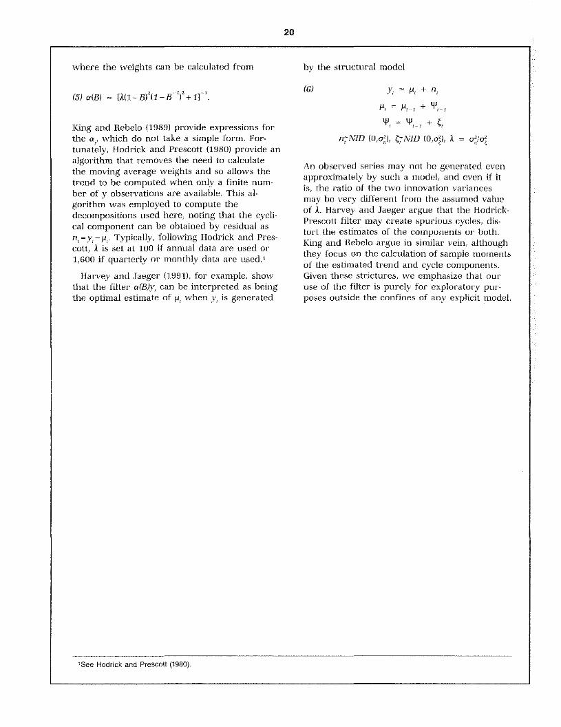
King and Rebelo (1989) provide expressions forthe a1, which do not take a simple form. For-tunately, Hodrick and Prescott (1980) provide analgorithm that removes the need to calculatethe moving average weights and so allows thetrend to he computed when only a finite num-ber of y observations are available. This al-gorithm was employed to compute thedecompositions used here, noting that the cycli-cal component can be obtained by residual as

‘~=v — p. Typically, following Hodrick and Pres-cott, A is set at 100 if annual data are used or1,600 if quarterly or monthly data are used.’

Harvey and Jaeger (1991), for example, showthat the filter a(BLv, can be interpreted as beingthe optimal estimate of p when y, is generated

by the structural model

(6) = ji, +

P, = +

Pr =4Jr~i +

rçNID (0,02), ~~NID ~~,°V’A =

An observed series may not be generated evenapproximately by such a model, and even if itis, the ratio of the two innovation vat’iancesmay be very different from the assumed valueof A. Harvey and Jaeger argue that the Hodrick-Prescott filter may create spurious cycles, dis-tort the estimates of the components or both.King and Rebelo argue in similar vein, althoughthey focus on the calculation of sample momentsof the estimated trend and cycle components.Given these strictures, we emphasize that ouruse of the filter is purely for explor’atory pur-poses outside the confines of any explicit model.

‘See Hodrick and Prescott (1980).