parameterized post-newtonian limit of horndeski’s gravity theory - …kodu.ut.ee › ~manuel ›...

Parameterized post-Newtonian limitof Horndeski’s gravity theory

Phys. Rev. D 92 064019

Manuel Hohmann

Laboratory of Theoretical PhysicsInstitute of PhysicsUniversity of Tartu

13. January 2016

Manuel Hohmann (University of Tartu) Horndeski PPN - Phys. Rev. D 92 064019 13. January 2016 1 / 29

Overview

1 Introduction

2 Massive scalar field

3 Massless scalar field

4 Experimental consistency

5 Particular models

6 Conclusion

Overview

1 Introduction

5 Particular models

6 Conclusion

Motivation

So far unexplained cosmological observations:Accelerating expansion of the universeHomogeneity of cosmic microwave background

Models for explaining these observations:ΛCDM model / dark energyInflation

Physical mechanisms are not understood:Unknown type of matter?Modification of the laws of gravity?

Scalar field in addition to metric mediating gravity?

Quantum gravity effects?

Horndeski gravity [G. W. Horndeski ’74]:Scalar-tensor theory of gravity.Most general STG with second order field equations.Healthy, ghost-free theory.Contains many interesting cases (Galileons, Higgs inflation. . . ).

Motivation

Physical mechanisms are not understood:Unknown type of matter?Modification of the laws of gravity?

Scalar field in addition to metric mediating gravity?

Quantum gravity effects?

Motivation

Physical mechanisms are not understood:Unknown type of matter?Modification of the laws of gravity?Scalar field in addition to metric mediating gravity?Quantum gravity effects?

Motivation

Physical mechanisms are not understood:Unknown type of matter?Modification of the laws of gravity?Scalar field in addition to metric mediating gravity?Quantum gravity effects?

Context: scalar-tensor theories of gravity

Appear as effective theories of more fundamental models:Low-energy limit of string theoryBraneworld models

“Classical” scalar tensor theories:Action:

∫d4x√−g[A(φ)R − B(φ)gµν∇µφ∇νφ− 2

[e2α(φ)gµν , χm

PPN parameters γ and β calculated [MH, L. Järv, P. Kuusk, E. Randla ’13].Invariance of the action under conformal transformations:

Different functions A,B,V, α describe the same theory.PPN parameters expressed by invariants [L. Järv, P. Kuusk, M. Saal, O. Vilson ’15].

Horndeski’s theory: generalizes aforementioned theories.

PPN parameters γ and β calculated [MH, L. Järv, P. Kuusk, E. Randla ’13].

Invariance of the action under conformal transformations:Different functions A,B,V, α describe the same theory.PPN parameters expressed by invariants [L. Järv, P. Kuusk, M. Saal, O. Vilson ’15].

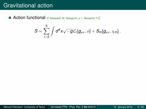
Gravitational action

Action functional [T. Kobayashi, M. Yamaguchi, J. ’i. Yokoyama ’11]:

S =5∑

∫d4x√−gLi [gµν , φ] + Sm[gµν , χm] .

Gravitational Lagrangian with X = −∇µφ∇µφ/2:

L2 = K (φ,X ) ,

L3 = −G3(φ,X )�φ ,

L4 = G4(φ,X )R + G4X (φ,X )[(�φ)2 − (∇µ∇νφ)2

L5 = G5(φ,X )Gµν∇µ∇νφ

− 16

G5X (φ,X )[(�φ)3 − 3(�φ)(∇µ∇νφ)2 + 2(∇µ∇νφ)3

Free functions K ,G3,G4,G5.

S =5∑

L2 = K (φ,X ) ,

L3 = −G3(φ,X )�φ ,

L4 = G4(φ,X )R + G4X (φ,X )[(�φ)2 − (∇µ∇νφ)2

− 16

G5X (φ,X )[(�φ)3 − 3(�φ)(∇µ∇νφ)2 + 2(∇µ∇νφ)3

S =5∑

L2 = K (φ,X ) ,

L3 = −G3(φ,X )�φ ,

L4 = G4(φ,X )R + G4X (φ,X )[(�φ)2 − (∇µ∇νφ)2

− 16

G5X (φ,X )[(�φ)3 − 3(�φ)(∇µ∇νφ)2 + 2(∇µ∇νφ)3

Field equations

Structure of the field equations:

5∑i=2

G iµν =

Tµν ,5∑

∇µJ iµ =

5∑i=2

P iφ .

More convenient: trace-reversed field equations:

5∑i=2

Riµν =

T̄µν =12

(Tµν −

gµνT).

Geometry tensors:

Riµν = G i

µν −12

gµνgρσG iρσ .

Field equations

5∑i=2

G iµν =

Tµν ,5∑

∇µJ iµ =

5∑i=2

P iφ .

5∑i=2

Riµν =

T̄µν =12

(Tµν −

gµνT).

Geometry tensors:

Riµν = G i

µν −12

gµνgρσG iρσ .

Field equations

5∑i=2

G iµν =

Tµν ,5∑

∇µJ iµ =

5∑i=2

P iφ .

5∑i=2

Riµν =

T̄µν =12

(Tµν −

gµνT).

Geometry tensors:

Riµν = G i

µν −12

gµνgρσG iρσ .

Perturbative expansion

Background solution:Minkowski metric ηµνConstant scalar field value Φ

Perturbation of dynamical fields:

gµν = ηµν + hµν , φ = Φ + ψ , X = −12∇µψ∇µψ .

Taylor expansion of free functions:

K (φ,X ) =∞∑

K(m,n)ψmX n .

Expansion coefficients:

K(m,n) =1

∂m+n

∂φm∂X n K (φ,X )

∣∣∣∣φ=Φ,X=0

Similar expansion for G3,G4,G5.

K (φ,X ) =∞∑

K(m,n)ψmX n .

K(m,n) =1

∂m+n

∣∣∣∣φ=Φ,X=0

K (φ,X ) =∞∑

K(m,n)ψmX n .

K(m,n) =1

∂m+n

∣∣∣∣φ=Φ,X=0

Post-Newtonian approximation

Perfect fluid energy-momentum tensor:

Tµν = (ρ+ ρΠ + p)uµuν + pgµν .Four-velocity uµ.Matter density ρ.Specific internal energy Π.Pressure p.

Slow-moving source matter:

v i =ui

u0 � 1 .

Assign velocity orders |v i |n ∼ O(n) based on solar system.Relevant terms for dynamical fields:

g00 = −1 + h(2)00 + h(4)

00 +O(6) , g0j = h(3)0j +O(5) ,

gij = δij + h(2)ij +O(4) , φ = Φ + ψ(2) + ψ(4) +O(6) .

Time dependence only through motion of source matter.⇒ Assign time derivative ∂0 ∼ O(1).

Tµν = (ρ+ ρΠ + p)uµuν + pgµν .Four-velocity uµ.Matter density ρ ∼ O(2).Specific internal energy Π ∼ O(2).Pressure p ∼ O(4).

v i =ui

u0 � 1 .

Assign velocity orders |v i |n ∼ O(n) based on solar system.

Relevant terms for dynamical fields:

g00 = −1 + h(2)00 + h(4)

00 +O(6) , g0j = h(3)0j +O(5) ,

v i =ui

u0 � 1 .

g00 = −1 + h(2)00 + h(4)

00 +O(6) , g0j = h(3)0j +O(5) ,

v i =ui

u0 � 1 .

g00 = −1 + h(2)00 + h(4)

00 +O(6) , g0j = h(3)0j +O(5) ,

Overview

1 Introduction

5 Particular models

6 Conclusion

Spherically symmetric solution

Static, point-like mass source:

ρ = Mδ(~x) , Π = 0 , p = 0 , vi = 0 .

Spherically symmetric metric:

g00 = −1 + 2Geff(r)U(r)− 2G2eff(r)β(r)U2(r) + Φ(4)(r) +O(6) ,

g0j = O(5) ,

gij = [1 + 2Geff(r)γ(r)U(r)] δij +O(4) .

Newtonian potential: U(r) = M/r .Gravitational self energy Φ(4)(r).Effective gravitational constant Geff(r).PPN parameters γ(r) and β(r).

Consistency condition:

K(0,0) = K(1,0) = 0 .

ρ = Mδ(~x) , Π = 0 , p = 0 , vi = 0 .

g0j = O(5) ,

K(0,0) = K(1,0) = 0 .

ρ = Mδ(~x) , Π = 0 , p = 0 , vi = 0 .

g0j = O(5) ,

K(0,0) = K(1,0) = 0 .

Scalar field ψ(2)

Scalar field equation at O(2) is screened Poisson equation:

ψ(2),ii −mψ

2ψ(2) = −cψρ .

Solution:ψ(2)(r) =

cψe−mψr .

Constants:

√√√√ −2K(2,0)

K(0,1) − 2G3(1,0) + 3G2

4(1,0)

G4(0,0)

cψ =G4(1,0)

2G4(0,0)

(K(0,1) − 2G3(1,0) + 3

G24(1,0)

G4(0,0)

Scalar field ψ(2)

ψ(2),ii −mψ

2ψ(2) = −cψρ .

Solution:ψ(2)(r) =

cψe−mψr .

Constants:

√√√√ −2K(2,0)

K(0,1) − 2G3(1,0) + 3G2

4(1,0)

G4(0,0)

cψ =G4(1,0)

2G4(0,0)

(K(0,1) − 2G3(1,0) + 3

G24(1,0)

G4(0,0)

Scalar field ψ(2)

ψ(2),ii −mψ

2ψ(2) = −cψρ .

Solution:ψ(2)(r) =

cψe−mψr .

Constants:

√√√√ −2K(2,0)

K(0,1) − 2G3(1,0) + 3G2

4(1,0)

G4(0,0)

cψ =G4(1,0)

2G4(0,0)

(K(0,1) − 2G3(1,0) + 3

G24(1,0)

G4(0,0)

Effective gravitational constant Geff(r)

Metric field equation:

h(2)00,ii = c1ψ

(2) − c2ρ .

Solve and read off effective gravitational constant:

Geff(r) =1

c1cψm2ψ

(e−mψr − 1)

Constants:

c1 = −2G4(1,0)K(2,0)

G4(0,0)

(K(0,1) − 2G3(1,0) + 3

G24(1,0)

G4(0,0)

4(1,0)

2G4(0,0)

(K(0,1) − 2G3(1,0) + 3

G24(1,0)

G4(0,0)

)−1 .

h(2)00,ii = c1ψ

(2) − c2ρ .

Geff(r) =1

c1cψm2ψ

(e−mψr − 1)

Constants:

c1 = −2G4(1,0)K(2,0)

G4(0,0)

(K(0,1) − 2G3(1,0) + 3

G24(1,0)

G4(0,0)

4(1,0)

2G4(0,0)

(K(0,1) − 2G3(1,0) + 3

G24(1,0)

G4(0,0)

)−1 .

h(2)00,ii = c1ψ

(2) − c2ρ .

Geff(r) =1

c1cψm2ψ

(e−mψr − 1)

Constants:

c1 = −2G4(1,0)K(2,0)

G4(0,0)

(K(0,1) − 2G3(1,0) + 3

G24(1,0)

G4(0,0)

4(1,0)

2G4(0,0)

(K(0,1) − 2G3(1,0) + 3

G24(1,0)

G4(0,0)

)−1 .

PPN parameter γ

h(2)ij,kk =

(2) − c4ρ)δij .

Solve and read off PPN parameter γ:

γ(r) =c4 +

c3cψm2ψ

(e−mψr − 1)

c2 +c1cψm2ψ

(e−mψr − 1).

Constants:

c3 = 2G4(1,0)K(2,0)

G4(0,0)

(K(0,1) − 2G3(1,0) + 3

G24(1,0)

G4(0,0)

G24(1,0)

2G4(0,0)

(K(0,1) − 2G3(1,0) + 3

G24(1,0)

G4(0,0)

)−1 .

PPN parameter γ

h(2)ij,kk =

(2) − c4ρ)δij .

γ(r) =c4 +

c3cψm2ψ

(e−mψr − 1)

c2 +c1cψm2ψ

(e−mψr − 1).

Constants:

c3 = 2G4(1,0)K(2,0)

G4(0,0)

(K(0,1) − 2G3(1,0) + 3

G24(1,0)

G4(0,0)

G24(1,0)

2G4(0,0)

(K(0,1) − 2G3(1,0) + 3

G24(1,0)

G4(0,0)

)−1 .

PPN parameter γ

h(2)ij,kk =

(2) − c4ρ)δij .

γ(r) =c4 +

c3cψm2ψ

(e−mψr − 1)

c2 +c1cψm2ψ

(e−mψr − 1).

Constants:

c3 = 2G4(1,0)K(2,0)

G4(0,0)

(K(0,1) − 2G3(1,0) + 3

G24(1,0)

G4(0,0)

G24(1,0)

2G4(0,0)

(K(0,1) − 2G3(1,0) + 3

G24(1,0)

G4(0,0)

)−1 .

PPN parameter γ

h(2)ij,kk =

(2) − c4ρ)δij .

γ(r) =2ω + 3− e−mψr

2ω + 3 + e−mψr .

Constants:

ω =G4(0,0)

2G24(1,0)

(K(0,1) − 2G3(1,0)

√√√√ −2K(2,0)

K(0,1) − 2G3(1,0) + 3G2

4(1,0)

G4(0,0)

PPN parameter β

Calculate β from fourth order solution:

β(r) = 1 +1

(2ω + 3 + e−mψr )2

{ω + τ − 4ωσ

2ω + 3e−2mψr

+ (2ω + 3)mψr[e−mψr ln(mψr)− 1

2e−2mψr

− (mψr + emψr ) Ei(−2mψr)

6µr + 3(3ω + τ + 6σ + 3)mψ2r

2(2ω + 3)mψ

[emψr Ei(−3mψr)

− e−mψr Ei(−mψr)]}

Constants mψ, ω, τ , σ, µ.

PPN parameter β

Calculate β from fourth order solution:

β(r) = 1 +1

(2ω + 3 + e−mψr )2

{ω + τ − 4ωσ

2ω + 3e−2mψr

+ (2ω + 3)mψr[e−mψr ln(mψr)− 1

2e−2mψr

− (mψr + emψr ) Ei(−2mψr)

6µr + 3(3ω + τ + 6σ + 3)mψ2r

2(2ω + 3)mψ

[emψr Ei(−3mψr)

− e−mψr Ei(−mψr)]}

Constants mψ, ω, τ , σ, µ.

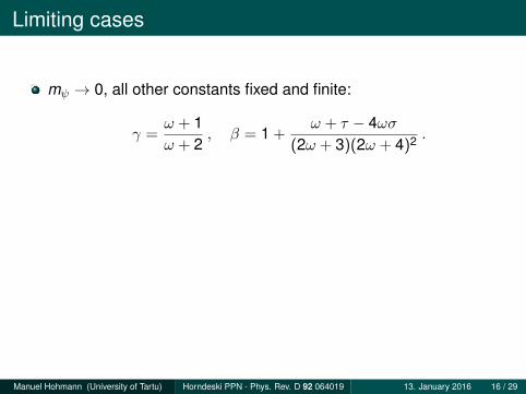
Limiting cases

mψ → 0, all other constants fixed and finite:

γ =ω + 1ω + 2

, β = 1 +ω + τ − 4ωσ

(2ω + 3)(2ω + 4)2 .

ω →∞, all other constants fixed and finite:

γ = β = 1 .

mψr →∞, large distance from the matter source:

γ = β = 1 .

Limiting cases

γ =ω + 1ω + 2

, β = 1 +ω + τ − 4ωσ

(2ω + 3)(2ω + 4)2 .

γ = β = 1 .

Limiting cases

γ =ω + 1ω + 2

, β = 1 +ω + τ − 4ωσ

(2ω + 3)(2ω + 4)2 .

γ = β = 1 .

Overview

1 Introduction

5 Particular models

6 Conclusion

Full PPN parameters for massless theory

Consider more restricted theory:

K(2,0) = K(3,0) = 0 .

⇒ All mass-like terms for ψ vanish.

⇒ PPN limit assumes standard form with constant PPN parameters.PPN parameters:

γ =ω + 1ω + 2

, β = 1 +ω + τ − 4ωσ

4(ω + 2)2(2ω + 3),

α1 = α2 = α3 = ζ1 = ζ2 = ζ3 = ζ4 = ξ = 0 .

⇒ Only γ and β potentially deviate from observed values.

Full PPN parameters for massless theory

Consider more restricted theory:

K(2,0) = K(3,0) = 0 .

⇒ All mass-like terms for ψ vanish.⇒ PPN limit assumes standard form with constant PPN parameters.

PPN parameters:

γ =ω + 1ω + 2

, β = 1 +ω + τ − 4ωσ

4(ω + 2)2(2ω + 3),

α1 = α2 = α3 = ζ1 = ζ2 = ζ3 = ζ4 = ξ = 0 .

⇒ Only γ and β potentially deviate from observed values.

Overview

1 Introduction

5 Particular models

6 Conclusion

Large mass limit

Asymptotic behavior of exponential integral:

Ei(−x) ≈ e−x

(1− 1!

x2 −3!

x3 + . . .

⇒ Terms involving σ, τ , µ ∼ e−2mψr are subleading.⇒ Consider simplified PPN parameters for mψr � 1:

γ(r) = 1− 22ω + 3

e−mψr +O(e−2mψr ) ,

β(r) = 1 +mψr

2ω + 3ln(mψr)e−mψr +O(e−2mψr ) .

Only depend on constants mψ, ω.⇒ Need experiments with fixed interaction distance r .

Most stringent bounds from Cassini tracking [B. Bertotti, L. Iess, P. Tortora ’03]:

γ − 1 = (2.1± 2.3) · 10−5 at r ≈ 7.44 · 10−3AU .

Large mass limit

Ei(−x) ≈ e−x

(1− 1!

x2 −3!

x3 + . . .

γ(r) = 1− 22ω + 3

β(r) = 1 +mψr

Only depend on constants mψ, ω.

⇒ Need experiments with fixed interaction distance r .Most stringent bounds from Cassini tracking [B. Bertotti, L. Iess, P. Tortora ’03]:

γ − 1 = (2.1± 2.3) · 10−5 at r ≈ 7.44 · 10−3AU .

Large mass limit

Ei(−x) ≈ e−x

(1− 1!

x2 −3!

x3 + . . .

γ(r) = 1− 22ω + 3

β(r) = 1 +mψr

Only depend on constants mψ, ω.⇒ Need experiments with fixed interaction distance r .

Most stringent bounds from Cassini tracking [B. Bertotti, L. Iess, P. Tortora ’03]:

γ − 1 = (2.1± 2.3) · 10−5 at r ≈ 7.44 · 10−3AU .

Excluded parameter ranges at 2σ

Small mass limit

PPN parameters independent of r for mψr � 1:

γ =ω + 1ω + 2

, β = 1 +ω + τ − 4ωσ

4(ω + 2)2(2ω + 3).

⇒ Possible to use observations where r is not well-defined.INPOP13 ephemeris [A. Fienga, P. Exertier, M. Gastineau, J. Laskar, H. Manche, A. Verma ’13/’14]:

γ − 1 = (−0.3± 2.5) · 10−5 , β − 1 = (0.2± 2.5) · 10−5 .

Still more stringent bounds by including Cassini tracking:

−2.5 · 1010 ≤ τ − 4ωσ ≤ 2.7 · 1010 for ω = 4.0 · 104 .

Less stringent bounds for larger values of ω.

Small mass limit

γ =ω + 1ω + 2

, β = 1 +ω + τ − 4ωσ

4(ω + 2)2(2ω + 3).

γ − 1 = (−0.3± 2.5) · 10−5 , β − 1 = (0.2± 2.5) · 10−5 .

−2.5 · 1010 ≤ τ − 4ωσ ≤ 2.7 · 1010 for ω = 4.0 · 104 .

Small mass limit

γ =ω + 1ω + 2

, β = 1 +ω + τ − 4ωσ

4(ω + 2)2(2ω + 3).

γ − 1 = (−0.3± 2.5) · 10−5 , β − 1 = (0.2± 2.5) · 10−5 .

−2.5 · 1010 ≤ τ − 4ωσ ≤ 2.7 · 1010 for ω = 4.0 · 104 .

How to get better bounds?

Stringency of bounds depends on interaction distance r0.Experiments with smaller r0 are more sensitive to mψ > 0.Measure γ and β at shorter distances.Earth-moon system? Satellite missions?

Can lunar laser ranging help?Nordvedt effect depends on γ and β.But: Nordvedt effect concerns motion in solar gravitational field.Interaction distance r0 = 1AU is large.Not the kind of experiment we need.

How to get better bounds?

Stringency of bounds depends on interaction distance r0.Experiments with smaller r0 are more sensitive to mψ > 0.Measure γ and β at shorter distances.Earth-moon system? Satellite missions?

Can lunar laser ranging help?Nordvedt effect depends on γ and β.But: Nordvedt effect concerns motion in solar gravitational field.Interaction distance r0 = 1AU is large.Not the kind of experiment we need.

Overview

1 Introduction

5 Particular models

6 Conclusion

Scalar-tensor gravity with potential

Gravitational action:

∫d4x√−g(φR − ω(φ)

φ∂ρφ∂

ρφ− 2κ2V (φ)

PPN parameters [MH, L. Järv, P. Kuusk, E. Randla ’13]:

γ(r) =2ω0 + 3− e−mψr

2ω0 + 3 + e−mψr ,

β(r) = 1 +1

(2ω0 + 3 + e−mψr )2

{Φω1

2ω0 + 3e−2mψr + (2ω0 + 3)mψr

×[e−mψr ln(mψr)− (mψr + emψr ) Ei(−2mψr)− 1

2e−2mψr

3mψr2

(1− ΦV3

2ω0 + 3

)[emψr Ei(−3mψr)− e−mψr Ei(−mψr)

Scalar-tensor gravity with potential

Gravitational action:

∫d4x√−g(φR − ω(φ)

φ∂ρφ∂

ρφ− 2κ2V (φ)

PPN parameters [MH, L. Järv, P. Kuusk, E. Randla ’13]:

γ(r) =2ω0 + 3− e−mψr

2ω0 + 3 + e−mψr ,

β(r) = 1 +1

(2ω0 + 3 + e−mψr )2

{Φω1

2ω0 + 3e−2mψr + (2ω0 + 3)mψr

×[e−mψr ln(mψr)− (mψr + emψr ) Ei(−2mψr)− 1

2e−2mψr

3mψr2

(1− ΦV3

2ω0 + 3

)[emψr Ei(−3mψr)− e−mψr Ei(−mψr)

Non-minimal Higgs inflation

Gravitational action [F. L. Bezrukov, M. Shaposhnikov ’08]:

∫d4x√−g

Pl − ξφ2

2R + X − V (φ)

PPN parameters:

γ = 1− 4ξ2e−mψr Φ2

β = 1 +{

2ξ3e−2mψr − ξ2mψr[e−2mψr − 2e−mψr ln(mψr)

+2(mψr + emψr )Ei(−2mψr)]} Φ2

Higgs field: mψ = 125GeV, Φ = 246GeV.⇒ γ = β = 1 on any astrophysical scale.

∫d4x√−g

Pl − ξφ2

2R + X − V (φ)

PPN parameters:

γ = 1− 4ξ2e−mψr Φ2

β = 1 +{

∫d4x√−g

Pl − ξφ2

2R + X − V (φ)

PPN parameters:

γ = 1− 4ξ2e−mψr Φ2

β = 1 +{

Overview

1 Introduction

5 Particular models

6 Conclusion

Summary

Horndeski’s gravity theory:Most general scalar-tensor theory with second order equations.Four free functions of φ and X = −∇µφ∇µφ/2.

Example theories:Classical scalar-tensor gravity with arbitrary potential.Models of Higgs inflation.Galileons.

PPN parameters:Most general theory: obtained PPN parameters γ(r) and β(r).Massless scalar field: only γ and β potentially deviate.Reproduces and generalizes well-known results.Many example theories compatible with solar system observations.

Summary

Outlook

Extend analysis to more general theories:Allow time-dependent scalar background field Φ̇ 6= 0.Theories beyond Horndeski / G3-inflation.Multi-scalar Horndeski gravity.

Take screening mechanisms into account:Vainshtein mechanism.Chameleon mechanism.Symmetron mechanism.

Outlook

Extend analysis to more general theories:Allow time-dependent scalar background field Φ̇ 6= 0.Theories beyond Horndeski / G3-inflation.Multi-scalar Horndeski gravity.

Take screening mechanisms into account:Vainshtein mechanism.Chameleon mechanism.Symmetron mechanism.

parameterized post-newtonian limit of horndeski’s gravity theory - …kodu.ut.ee › ~manuel ›...

Documents