package ‘limsolve’ limsolve ... (system.file(package="limsolve"), "/doc",...

Package ‘limSolve’August 14, 2017

Version 1.5.5.3

Title Solving Linear Inverse Models

Author Karline Soetaert [aut, cre],Karel Van den Meersche [aut],Dick van Oevelen [aut],LAPACK authors [cph]

Maintainer Karline Soetaert <[email protected]>

Depends R (>= 2.10)

Imports quadprog, lpSolve, MASS

Description Functions that (1) find the minimum/maximum of a linear or quadratic function:min or max (f(x)), where f(x) = ||Ax-b||^2 or f(x) = sum(a_i*x_i)subject to equality constraints Ex=f and/or inequality constraints Gx>=h,(2) sample an underdetermined-or overdetermined system Ex=f subject to Gx>=h, and if applicable Ax~=b,(3) solve a linear system Ax=B for the unknown x. It includes banded and tridiagonal linear sys-tems.The package calls Fortran functions from 'LINPACK'.

License GPL

Copyright inst/COPYRIGHTS

LazyData yes

Repository CRAN

Repository/R-Forge/Project limsolve

Repository/R-Forge/Revision 115

Repository/R-Forge/DateTimeStamp 2017-08-14 11:40:30

Date/Publication 2017-08-14 15:14:43 UTC

NeedsCompilation yes

R topics documented:limSolve-package . . . . . . . . . . . . . . . . . . . . . . . . . . . . . . . . . . . . . . 2Blending . . . . . . . . . . . . . . . . . . . . . . . . . . . . . . . . . . . . . . . . . . . 4

1

2 limSolve-package

Chemtax . . . . . . . . . . . . . . . . . . . . . . . . . . . . . . . . . . . . . . . . . . . 6E_coli . . . . . . . . . . . . . . . . . . . . . . . . . . . . . . . . . . . . . . . . . . . . 9ldei . . . . . . . . . . . . . . . . . . . . . . . . . . . . . . . . . . . . . . . . . . . . . 11ldp . . . . . . . . . . . . . . . . . . . . . . . . . . . . . . . . . . . . . . . . . . . . . . 14linp . . . . . . . . . . . . . . . . . . . . . . . . . . . . . . . . . . . . . . . . . . . . . 15lsei . . . . . . . . . . . . . . . . . . . . . . . . . . . . . . . . . . . . . . . . . . . . . . 18Minkdiet . . . . . . . . . . . . . . . . . . . . . . . . . . . . . . . . . . . . . . . . . . . 21nnls . . . . . . . . . . . . . . . . . . . . . . . . . . . . . . . . . . . . . . . . . . . . . 24resolution . . . . . . . . . . . . . . . . . . . . . . . . . . . . . . . . . . . . . . . . . . 25RigaWeb . . . . . . . . . . . . . . . . . . . . . . . . . . . . . . . . . . . . . . . . . . . 26Solve . . . . . . . . . . . . . . . . . . . . . . . . . . . . . . . . . . . . . . . . . . . . 28Solve.banded . . . . . . . . . . . . . . . . . . . . . . . . . . . . . . . . . . . . . . . . 29Solve.block . . . . . . . . . . . . . . . . . . . . . . . . . . . . . . . . . . . . . . . . . 31Solve.tridiag . . . . . . . . . . . . . . . . . . . . . . . . . . . . . . . . . . . . . . . . . 33varranges . . . . . . . . . . . . . . . . . . . . . . . . . . . . . . . . . . . . . . . . . . 35varsample . . . . . . . . . . . . . . . . . . . . . . . . . . . . . . . . . . . . . . . . . . 36xranges . . . . . . . . . . . . . . . . . . . . . . . . . . . . . . . . . . . . . . . . . . . 38xsample . . . . . . . . . . . . . . . . . . . . . . . . . . . . . . . . . . . . . . . . . . . 39

Index 44

limSolve-package Solving Linear Inverse Models

Description

Functions that:

(1.) Find the minimum/maximum of a linear or quadratic function: min or max (f(x)), wheref(x) = ||Ax − b||2 or f(x) = sum(ai ∗ xi) subject to equality constraints Ex = f and/orinequality constraints Gx >= h.

(2.) Sample an underdetermined- or overdetermined system Ex = f subject to Gx >= h, and ifapplicable Ax = b.

(3.) Solve a linear system Ax = B for the unknown x. Includes banded and tridiagonal linearsystems.

The package calls Fortran functions from LINPACK

Details

Package: limSolveType: PackageVersion: 1.5.4Date: 2013-23-01License: GNU Public License 2 or above

limSolve is designed for solving linear inverse models (LIM).

limSolve-package 3

These consist of linear equality and, or inequality conditions, which can be solved either by leastsquares or by linear programming techniques.

Amongst the possible applications are: food web quantification, flux balance analysis (e.g. metabolicnetworks), compositional estimation, and operations research problems.

The package contains several examples to exemplify its use

Author(s)

Karline Soetaert (Maintainer),

Karel Van den Meersche

Dick van Oevelen

References

Van den Meersche K, Soetaert K, Van Oevelen D (2009). xsample(): An R Function for SamplingLinear Inverse Problems. Journal of Statistical Software, Code Snippets, 30(1), 1-15.

http://www.jstatsoft.org/v30/c01/

See Also

Blending, Chemtax, RigaWeb, E_coli, Minkdiet the examples.

ldei, lsei,linp, ldp, nnls to solve LIM

xranges, varranges to estimate ranges of unknowns and variables

xsample, varsample to create a random sample of unknowns and variables

Solve, Solve.banded, Solve.tridiag, to solve non-square, banded and tridiagonal linear systemsof equations.

resolution row and column resolution of a matrix

package vignette limSolve

Examples

## Not run:## show examples (see respective help pages for details)example(Blending)example(Chemtax)example(E_coli)example(Minkdiet)

## run demosdemo("limSolve")

## open the directory with original E_coli input filebrowseURL(paste(system.file(package="limSolve"), "/doc", sep=""))

## show package vignette with tutorial about xsamplevignette("xsample")


4 Blending

## show main package vignettevignette("limSolve")

## End(Not run)

Blending A linear inverse blending problem

Description

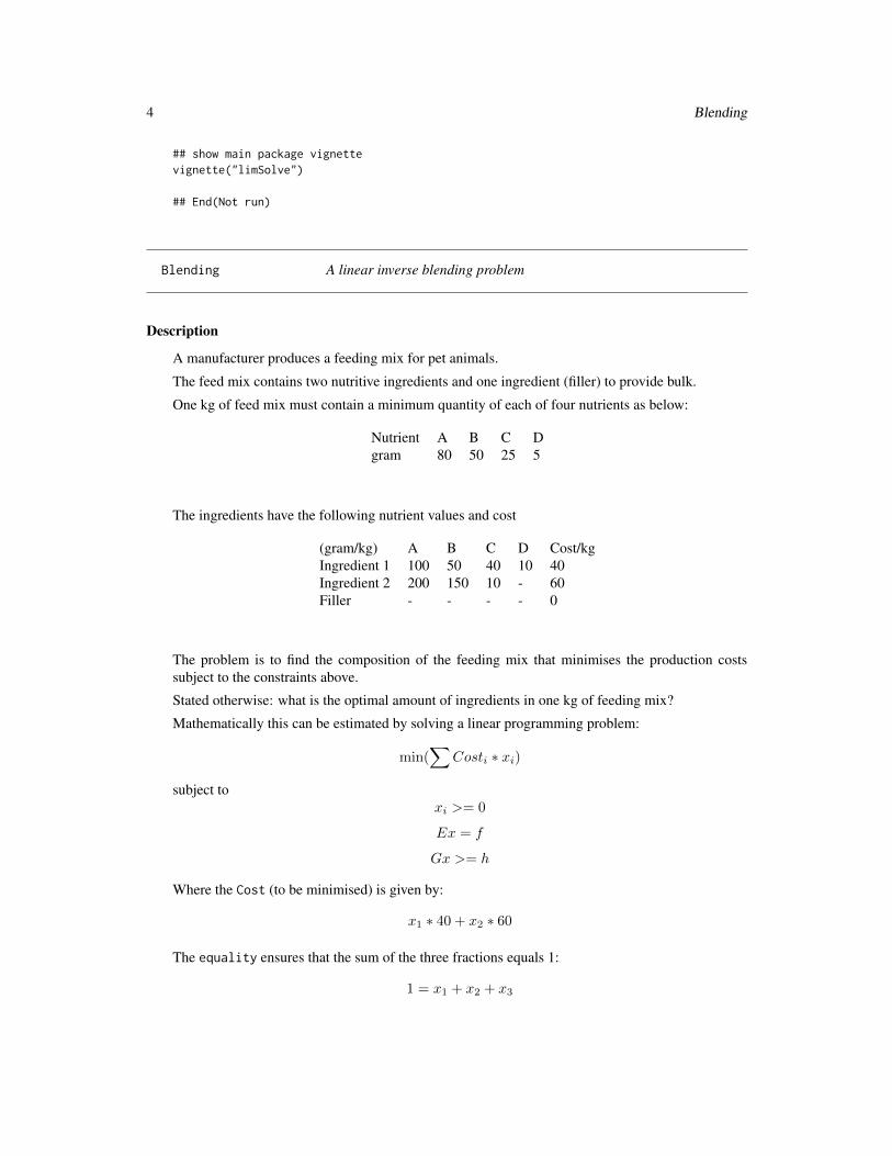
A manufacturer produces a feeding mix for pet animals.

The feed mix contains two nutritive ingredients and one ingredient (filler) to provide bulk.

One kg of feed mix must contain a minimum quantity of each of four nutrients as below:

Nutrient A B C Dgram 80 50 25 5

The ingredients have the following nutrient values and cost

(gram/kg) A B C D Cost/kgIngredient 1 100 50 40 10 40Ingredient 2 200 150 10 - 60Filler - - - - 0

The problem is to find the composition of the feeding mix that minimises the production costssubject to the constraints above.

Stated otherwise: what is the optimal amount of ingredients in one kg of feeding mix?

Mathematically this can be estimated by solving a linear programming problem:

min(∑

Costi ∗ xi)

subject toxi >= 0

Ex = f

Gx >= h

Where the Cost (to be minimised) is given by:

x1 ∗ 40 + x2 ∗ 60

The equality ensures that the sum of the three fractions equals 1:

1 = x1 + x2 + x3

Blending 5

And the inequalities enforce the nutritional constraints:

100 ∗ x1 + 200 ∗ x2 > 80

50 ∗ x1 + 150 ∗ x2 > 50

and so on

The solution is Ingredient1 (x1) = 0.5909, Ingredient2 (x2)=0.1364 and Filler (x3)=0.2727.

Usage

Blending

Format

A list with matrix G and vector H that contain the inequality conditions and with vector Cost, defin-ing the cost function.

Columnnames of G or names of Cost are the names of the ingredients, rownames of G and names ofH are the nutrients.

Author(s)

Karline Soetaert <[email protected]>.

See Also

linp to solve a linear programming problem.

Examples

# Generate the equality condition (sum of ingredients = 1)E <- rep(1, 3)F <- 1

G <- Blending$GH <- Blending$H

# add positivity requirementG <- rbind(G, diag(3))H <- c(H, rep(0, 3))

# 1. Solve the model with linear programmingres <- linp(E = t(E), F = F, G = G, H = H, Cost = Blending$Cost)

# show resultsprint(c(res$X, Cost = res$solutionNorm))

dotchart(x = as.vector(res$X), labels = colnames(G),main = "Optimal blending with ranges",sub = "using linp and xranges", pch = 16,xlim = c(0, 1))

6 Chemtax

# 2. Possible ranges of the three ingredients(xr <- xranges(E, F, G, H))segments(xr[,1], 1:ncol(G), xr[,2], 1:ncol(G))legend ("topright", pch = c(16, NA), lty = c(NA, 1),

legend = c("Minimal cost", "range"))

# 3. Random sample of the three ingredients# The inequality that all x > 0 has to be added!xs <- xsample(E = E, F = F, G = G, H = H)$X

pairs(xs, main = "Blending, 3000 solutions with xsample")

# Cost associated to these random samplesCosts <- as.vector(varsample(xs, EqA = Blending$Cost))hist(Costs)legend("topright", c("Optimal solution",

format(res$solutionNorm, digits = 3)))

Chemtax An overdetermined linear inverse problem: estimating algal composi-tion based on pigment biomarkers.

Description

Input files for assessing the algal composition of a field sample, based on the pigment compositionof the algal groups (measured in the laboratory) and the pigment composition of the field sample.

In the example there are 8 types of algae:

• Prasinophytes

• Dinoflagellates

• Cryptophytes

• Haptophytes type 3 (Hapto3s)

• Haptophytes type 4 (Hapto4s)

• Chlorophytes

• Cynechococcus

• Diatoms

and 12 pigments:

Perid = Peridinin, 19But = 19-butanoyloxyfucoxanthin, Fucox = fucoxanthin,

19Hex = 19-hexanoyloxyfucoxanthin, Neo = neoxanthin, Pras = prasinoxanthin,

Viol = violaxanthin, Allox = alloxanthin, Lutein = lutein,

Zeax = zeaxanthin, Chlb = chlorophyll b, Chla = chlorophyll a

The input data consist of:

Chemtax 7

1. the pigment composition of the various algal groups, for instance determined from cultures(the Southern Ocean example -table 4- in Mackey et al., 1996)

2. the pigment composition of a field sample.

Based on these data, the algal composition of the field sample is estimated, under the assumptionthat the pigment composition of the field sample is a weighted avertage of the pigment compositionof algae present in the sample, where weighting is proportional to their biomass.

As there are more measurements (12 pigments) than unknowns (8 algae), the resulting linear systemis overdetermined.

It is thus solved in a least squares sense (using function lsei):

min(||Ax− b||2)

subject toEx = f

Gx >= h

If there are 2 algae A,B, and 3 pigments 1,2,3 then the 3 approximate equalities (A∗x = B) wouldbe:

f1,S = pA ∗ fA,1 + pB ∗ fB,1

f2,S = pA ∗ fA,2 + pB ∗ fB,3

f3,S = pA ∗ fA,3 + pB ∗ fB,3

where pA and pb are the (unknown) proportions of algae A and B in the field sample (S), and fA,1

is the relative amount of pigment 1 in alga A, etc...

The equality ensures that the sum of fractions equals 1:

1 = pA + pb

and the inequalities ensure that fractions are positive numbers

pA > 0

pB > 0

It should be noted that in the actual Chemtax programme the problem is solved in a more complexway. In Chemtoz, the A-coefficients are also allowed to vary, while here they are taken as theyare (constant). Chemtax then finds the "best fit" by fitting both the fractions, and the non-zerocoefficients in A.

Usage

Chemtax

8 Chemtax

Format

A list with the input ratio matrix (Ratio) and a vector with the field data (Field)

• The input ratio matrix Ratio contains the pigment compositions (columns) for each algalgroup (rows); the compositions are scaled relative to Chla (last column).

• The vector with the Field data contains the pigment composition of a sample in the field, alsoscaled relative to Chla; the pigments are similarly ordened as for the input ratio matrix.

The rownames of matrix Ratio are the algal group names, columnames of Ratio (=names of Field)are the pigments

Author(s)


References

Mackey MD, Mackey DJ, Higgins HW, Wright SW, 1996. CHEMTAX - A program for estimatingclass abundances from chemical markers: Application to HPLC measurements of phytoplankton.Marine Ecology-Progress Series 144 (1-3): 265-283.

Van den Meersche, K., Soetaert, K., Middelburg, J., 2008. A Bayesian compositional estimator formicrobial taxonomy based on biomarkers. Limnology and Oceanography Methods, 6, 190-199.

R-package BCE

See Also

lsei, the function to solve for the algal composition of the field sample.

Examples

# 1. Graphical representation of the chemtax example input datapalette(rainbow(12, s = 0.6, v = 0.75))

mp <- apply(Chemtax$Ratio, MARGIN = 2, max)pstars <- rbind(t(t(Chemtax$Ratio)/mp) ,

sample = Chemtax$Field/max(Chemtax$Field))stars(pstars, len = 0.9, key.loc = c(7.2, 1.7),scale=FALSE,ncol=4,

main = "CHEMTAX pigment composition", draw.segments = TRUE,flip.labels=FALSE)

# 2. Estimating the algal composition of the field sampleNx <-nrow(Chemtax$Ratio)

# equations that have to be met exactly Ex=f:# sum of all fraction must be equal to 1.EE <- rep(1, Nx)FF <- 1

# inequalities, Gx>=h:# all fractions must be positive numbers

E_coli 9

GG <- diag(nrow = Nx)HH <- rep(0, Nx)

# equations that must be reproduced as close as possible, Ax ~ b# = the field data; the input ratio matrix and field data are rescaledAA <- Chemtax$Ratio/rowSums(Chemtax$Ratio)BB <- Chemtax$Field/sum(Chemtax$Field)

# 1. Solve with lsei methodX <- lsei(t(AA), BB, EE, FF, GG, HH)$X(Sample <- data.frame(Algae = rownames(Chemtax$Ratio),

fraction = X))

# plot resultsbarplot(X, names = rownames(Chemtax$Ratio), col = heat.colors(8),

cex.names = 0.8, main = "Chemtax example solved with lsei")

# 2. Bayesian sampling;# The standard deviation on the field data is assumed to be 0.01# jump length not too large or NO solutions are found!xs <- xsample(t(AA), BB, EE, FF, GG, HH, sdB = 0.01, jmp = 0.025)$Xpairs(xs, main= "Chemtax, Bayesian sample")

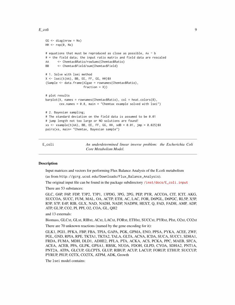
E_coli An underdetermined linear inverse problem: the Escherichia ColiCore Metabolism Model.

Description

Input matrices and vectors for performing Flux Balance Analysis of the E.coli metabolism

(as from http://gcrg.ucsd.edu/Downloads/Flux_Balance_Analysis).

The original input file can be found in the package subdirectory /inst/docs/E_coli.input

There are 53 substances:

GLC, G6P, F6P, FDP, T3P2, T3P1, 13PDG, 3PG, 2PG, PEP, PYR, ACCOA, CIT, ICIT, AKG,SUCCOA, SUCC, FUM, MAL, OA, ACTP, ETH, AC, LAC, FOR, D6PGL, D6PGC, RL5P, X5P,R5P, S7P, E4P, RIB, GLX, NAD, NADH, NADP, NADPH, HEXT, Q, FAD, FADH, AMP, ADP,ATP, GL3P, CO2, PI, PPI, O2, COA, GL, QH2

and 13 externals:

Biomass, GLCxt, GLxt, RIBxt, ACxt, LACxt, FORxt, ETHxt, SUCCxt, PYRxt, PIxt, O2xt, CO2xt

There are 70 unknown reactions (named by the gene encoding for it):

GLK1, PGI1, PFKA, FBP, FBA, TPIA, GAPA, PGK, GPMA, ENO, PPSA, PYKA, ACEE, ZWF,PGL, GND, RPIA, RPE, TKTA1, TKTA2, TALA, GLTA, ACNA, ICDA, SUCA, SUCC1, SDHA1,FRDA, FUMA, MDH, DLD1, ADHE2, PFLA, PTA, ACKA, ACS, PCKA, PPC, MAEB, SFCA,ACEA, ACEB, PPA, GLPK, GPSA1, RBSK, NUOA, FDOH, GLPD, CYOA, SDHA2, PNT1A,PNT2A, ATPA, GLCUP, GLCPTS, GLUP, RIBUP, ACUP, LACUP, FORUP, ETHUP, SUCCUP,PYRUP, PIUP, O2TX, CO2TX, ATPM, ADK, Growth

The lsei model contains:

/inst/docs/E_coli.input

10 E_coli

• 54 equalities (Ax=B): the 53 mass balances (one for each substance) and one equation thatsets the ATP drain flux for constant maintenance requirements to a fixed value (5.87)

• 70 unknowns (x), the reaction rates

• 62 inequalities (Gx>h). The first 28 inequalities impose bounds on some reactions. The last34 inequalities impose that the reaction rates have to be positive (for unidirectional reactionsonly).

• 1 function that has to be maximised, the biomass production (growth).

As there are more unknowns (70) than equations (54), there exist an infinite amount of solutions (itis an underdetermined problem).

Usage

E_coli

Format

A list with the matrices and vectors that constitute the mass balance problem: A, B, G and H and

Maximise, with the function to maximise.

The columnames of A and G are the names of the unknown reaction rates; The first 53 rownames ofA give the names of the components (these rows consitute the mass balance equations).

Author(s)

Karline Soetaert <[email protected]>

References

originated from the urlhttp://gcrg.ucsd.edu/Downloads/Flux_Balance_Analysis

Edwards,J.S., Covert, M., and Palsson, B., (2002) Metabolic Modeling of Microbes: the Flux Bal-ance Approach, Environmental Microbiology, 4(3): pp. 133-140.

Examples

# 1. parsimonious (simplest) solutionpars <- lsei(E = E_coli$A, F = E_coli$B, G = E_coli$G, H = E_coli$H)$X

# 2. the optimal solution - solved with linear programming# some unknowns can be negative

LP <- linp(E = E_coli$A, F = E_coli$B,G = E_coli$G, H = E_coli$H,Cost = -E_coli$Maximise, ispos = FALSE)

(Optimal <- LP$X)

# 3.ranges of all unknowns, including the central value and all solutionsxr <- xranges(E = E_coli$A, F = E_coli$B, G = E_coli$G, H = E_coli$H,

central = TRUE, full = TRUE)

# the central point is a valid solution:

ldei 11

X <- xr[ ,"central"]max(abs(E_coli$A%*%X - E_coli$B))min(E_coli$G%*%X - E_coli$H)

# 4. Sample solution space; the central value is a good starting point# for algorithms cda and rda - but these need many iterations## Not run:xs <- xsample(E = E_coli$A, F = E_coli$B, G = E_coli$G,H = E_coli$H,

iter = 50000, out = 5000, type = "rda", x0 = X)$Xpairs(xs[ ,10:20], pch = ".", cex = 2, main = "sampling, using rda")

## End(Not run)

# using mirror algorithm takes less iterations,# but an iteration takes more time ; it is better to start in a corner...# (i.e. no need to use X as starting value)xs <- xsample(E = E_coli$A, F = E_coli$B, G = E_coli$G, H = E_coli$H,

iter = 2000, out = 500, jmp = 50, type = "mirror")$Xpairs(xs[ ,10:20], pch = ".", cex = 2, main = "sampling, using mirror")

# Print results:data.frame(pars = pars, Optimal = Optimal, xr[ ,1:2],

Mean = colMeans(xs), sd = apply(xs, 2, sd))

# Plot resultspar(mfrow = c(1, 2))nr <- length(Optimal)/2

ii <- 1:nrdotchart(Optimal[ii], xlim = range(xr), pch = 16)segments(xr[ii,1], 1:nr, xr[ii,2], 1:nr)

ii <- (nr+1):length(Optimal)dotchart(Optimal[ii], xlim = range(xr), pch = 16)segments(xr[ii,1], 1:nr, xr[ii,2], 1:nr)mtext(side = 3, cex = 1.5, outer = TRUE, line = -1.5,

"E coli Core Metabolism, optimal solution and ranges")

ldei Weighted Least Distance Programming with equality and inequalityconstraints.

Description

Solves the following underdetermined inverse problem:

min(∑

xi2)

subject toEx = f

12 ldei

Gx >= h

uses least distance programming subroutine ldp (FORTRAN) from Linpack

The model has to be UNDERdetermined, i.e. the number of independent equations < number ofunknowns.

Usage

ldei(E, F, G = NULL, H = NULL,tol = sqrt(.Machine$double.eps), verbose = TRUE)

Arguments

E numeric matrix containing the coefficients of the equality constraints Ex = F ;if the columns of E have a names attribute, they will be used to label the output.

F numeric vector containing the right-hand side of the equality constraints.

G numeric matrix containing the coefficients of the inequality constraints Gx >=H; if the columns of G have a names attribute and the columns of E do not, theywill be used to label the output.

H numeric vector containing the right-hand side of the inequality constraints.

tol tolerance (for singular value decomposition, equality and inequality constraints).

verbose logical to print ldei error messages.

Value

a list containing:

X vector containing the solution of the least distance with equalities and inequali-ties problem.

unconstrained.solution

vector containing the unconstrained solution of the least distance problem, i.e.ignoring Gx >= h.

residualNorm scalar, the sum of absolute values of residuals of equalities and violated inequal-ities; should be zero or very small if the problem is feasible.

solutionNorm scalar, the value of the quadratic function at the solution, i.e. the value of∑wi ∗ xi

2.

IsError logical, TRUE if an error occurred.

type the string "ldei", such that how the solution was obtained can be traced.

numiter the number of iterations.

Note

One of the steps in the ldei algorithm is the creation of an orthogonal basis, constructed by SingularValue Decomposition. As this makes use of random numbers, it may happen - for problems thatare difficult to solve - that ldei sometimes finds a solution or fails to find one for the same problem,depending on the random numbers used to create the orthogonal basis. If it is suspected that this ishappening, trying a few times may find a solution. (example RigaWeb is such a problem).

ldei 13

Author(s)


References

Lawson C.L.and Hanson R.J. 1974. Solving Least Squares Problems, Prentice-Hall

Lawson C.L.and Hanson R.J. 1995. Solving Least Squares Problems. SIAM classics in appliedmathematics, Philadelphia. (reprint of book)

See Also

Minkdiet, for a description of the Mink diet example.

lsei, linp

ldp

Examples

#-------------------------------------------------------------------------------# A simple problem#-------------------------------------------------------------------------------# minimise x1^2 + x2^2 + x3^2 + x4^2 + x5^2 + x6^2# subject to:#-x1 + x4 + x5 = 0# - x2 - x4 + x6 = 0# x1 + x2 + x3 > 1# x3 + x5 + x6 < 1# xi > 0

E <- matrix(nrow = 2, byrow = TRUE, data = c(-1, 0, 0, 1, 1, 0,0,-1, 0, -1, 0, 1))

F <- c(0, 0)G <- matrix(nrow = 2, byrow = TRUE, data = c(1, 1, 1, 0, 0, 0,

0, 0, -1, 0, -1, -1))H <- c(1, -1)ldei(E, F, G, H)

#-------------------------------------------------------------------------------# parsimonious (simplest) solution of the mink diet problem#-------------------------------------------------------------------------------E <- rbind(Minkdiet$Prey, rep(1, 7))F <- c(Minkdiet$Mink, 1)

parsimonious <- ldei(E, F, G = diag(7), H = rep(0, 7))data.frame(food = colnames(Minkdiet$Prey),

fraction = parsimonious$X)dotchart(x = as.vector(parsimonious$X),

labels = colnames(Minkdiet$Prey),main = "Diet composition of Mink extimated using ldei",xlab = "fraction")

14 ldp

ldp Least Distance Programming

Description

Solves the following inverse problem:

min(∑

xi2)

subject toGx >= h

uses least distance programming subroutine ldp (FORTRAN) from Linpack

Usage

ldp(G, H, tol = sqrt(.Machine$double.eps), verbose = TRUE)

Arguments

G numeric matrix containing the coefficients of the inequality constraints Gx >=H; if the columns of G have a names attribute, they will be used to label theoutput.


tol tolerance (for inequality constraints).

verbose logical to print ldp error messages.

Value

a list containing:

X vector containing the solution of the least distance problem.

residualNorm scalar, the sum of absolute values of residuals of violated inequalities; should bezero or very small if the problem is feasible.

solutionNorm scalar, the value of the quadratic function at the solution, i.e. the value of∑wi ∗ xi

2.


type the string "ldp", such that how the solution was obtained can be traced.


Author(s)


linp 15

References



See Also

ldei, which includes equalities.

Examples

# parsimonious (simplest) solutionG <- matrix(nrow = 2, ncol = 2, data = c(3, 2, 2, 4))H <- c(3, 2)

ldp(G, H)

linp Linear Programming.

Description

Solves a linear programming problem,

min(∑

Costi.xi)

subject toEx = f

Gx >= h

xi >= 0

(optional)

This function provides a wrapper around lp (see note) from package lpSolve, written to be consis-tent with the functions lsei, and ldei.

It allows for the x’s to be negative (not standard in lp).

Usage

linp(E = NULL, F = NULL, G = NULL, H = NULL, Cost,ispos = TRUE, int.vec = NULL, verbose = TRUE, ...)

16 linp

Arguments

E numeric matrix containing the coefficients of the equality constraints Ex = F ;if the columns of E have a names attribute, they will be used to label the output.


G numeric matrix containing the coefficients of the inequality constraints Gx >=H; if the columns of G have a names attribute, and the columns of E do not, theywill be used to label the output.


Cost numeric vector containing the coefficients of the cost function; if Cost has anames attribute, and neither the columns of E nor G have a name, they will beused to label the output.

ispos logical, when TRUE then the unknowns (x) must be positive (this is consistentwith the original definition of a linear programming problem).

int.vec when not NULL, a numeric vector giving the indices of variables that are requiredto be an integer. The length of this vector will therefore be the number of integervariables.

verbose logical to print error messages.

... extra arguments passed to R-function lp.

Value

a list containing:

X vector containing the solution of the linear programming problem.

residualNorm scalar, the sum of absolute values of residuals of equalities and violated inequal-ities. Should be very small or zero for a feasible linear programming problem.

solutionNorm scalar, the value of the minimised Cost function, i.e. the value of∑

Costi.xi.


type the string "linp", such that how the solution was obtained can be traced.

Note

If the requirement of nonnegativity are relaxed, then strictly speaking the problem is not a linearprogramming problem.

The function lp may fail and terminate R for very small problems that are repeated frequently...

Also note that sometimes multiple solutions exist for the same problem.

Author(s)


References

Michel Berkelaar and others (2007). lpSolve: Interface to Lpsolve v. 5.5 to solve linear or integerprograms. R package version 5.5.8.

linp 17

See Also

ldei, lsei,

lp the original function from package lpSolve

Blending, a linear programming problem.

Examples

#-------------------------------------------------------------------------------# Linear programming problem 1, not feasible#-------------------------------------------------------------------------------

# maximise x1 + 3*x2# subject to#-x1 -x2 < -3#-x1 + x2 <-1# x1 + 2*x2 < 2# xi > 0

G <- matrix(nrow = 3, data = c(-1, -1, 1, -1, 1, 2))H <- c(3, -1, 2)Cost <- c(-1, -3)(L <- linp(E = NULL, F = NULL, Cost = Cost, G = G, H = H))L$residualNorm

#-------------------------------------------------------------------------------# Linear programming problem 2, feasible#-------------------------------------------------------------------------------

# minimise x1 + 8*x2 + 9*x3 + 2*x4 + 7*x5 + 3*x6# subject to:#-x1 + x4 + x5 = 0# - x2 - x4 + x6 = 0# x1 + x2 + x3 > 1# x3 + x5 + x6 < 1# xi > 0

E <- matrix(nrow = 2, byrow = TRUE, data = c(-1, 0, 0, 1, 1, 0,0,-1, 0, -1, 0, 1))

F <- c(0, 0)G <- matrix(nrow = 2, byrow = TRUE, data = c(1, 1, 1, 0, 0, 0,

0, 0, -1, 0, -1, -1))H <- c(1, -1)Cost <- c(1, 8, 9, 2, 7, 3)(L <- linp(E = E, F = F, Cost = Cost, G = G, H = H))L$residualNorm

#-------------------------------------------------------------------------------# Linear programming problem 3, no positivity#-------------------------------------------------------------------------------# minimise x1 + 2x2 -x3 +4 x4# subject to:

18 lsei

# 3x1 + 2x2 + x3 + x4 = 2# x1 + x2 + x3 + x4 = 2

# 2x1 + x2 + x3 + x4 >=-1# -x1 + 3x2 +2x3 + x4 >= 2# -x1 + x3 >= 1

E <- matrix(ncol = 4, byrow = TRUE,data =c(3, 2, 1, 4, 1, 1, 1, 1))

F <- c(2, 2)

G <- matrix(ncol = 4, byrow = TRUE,data = c(2, 1, 1, 1, -1, 3, 2, 1, -1, 0, 1, 0))

H <- c(-1, 2, 1)Cost <- c(1, 2, -1, 4)

linp(E = E, F = F, G = G, H = H, Cost, ispos = FALSE)

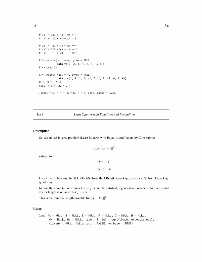
lsei Least Squares with Equalities and Inequalities

Description

Solves an lsei inverse problem (Least Squares with Equality and Inequality Constraints)

min(||Ax− b||2)

subject to

Ex = f

Gx >= h

Uses either subroutine lsei (FORTRAN) from the LINPACK package, or solve.QP from R-packagequadprog.

In case the equality constraints Ex = f cannot be satisfied, a generalized inverse solution residualvector length is obtained for f − Ex.

This is the minimal length possible for ||f − Ex||2.

Usage

lsei (A = NULL, B = NULL, E = NULL, F = NULL, G = NULL, H = NULL,Wx = NULL, Wa = NULL, type = 1, tol = sqrt(.Machine$double.eps),tolrank = NULL, fulloutput = FALSE, verbose = TRUE)

lsei 19

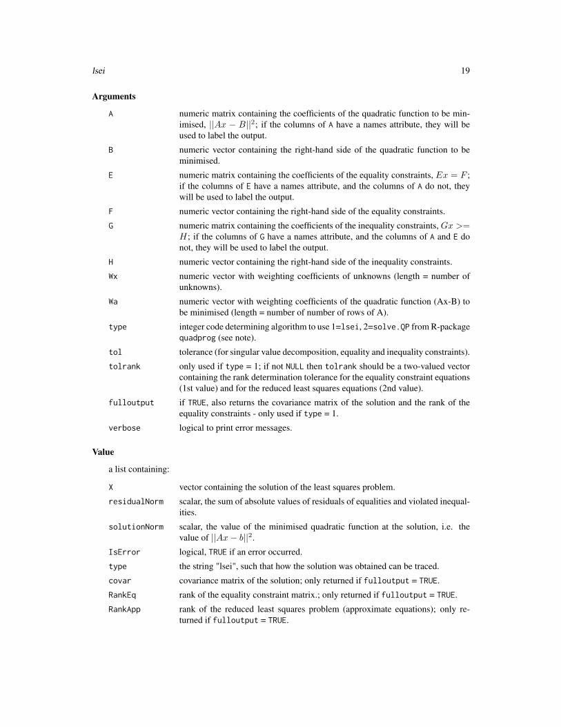
Arguments

A numeric matrix containing the coefficients of the quadratic function to be min-imised, ||Ax − B||2; if the columns of A have a names attribute, they will beused to label the output.

B numeric vector containing the right-hand side of the quadratic function to beminimised.

E numeric matrix containing the coefficients of the equality constraints, Ex = F ;if the columns of E have a names attribute, and the columns of A do not, theywill be used to label the output.


G numeric matrix containing the coefficients of the inequality constraints, Gx >=H; if the columns of G have a names attribute, and the columns of A and E donot, they will be used to label the output.


Wx numeric vector with weighting coefficients of unknowns (length = number ofunknowns).

Wa numeric vector with weighting coefficients of the quadratic function (Ax-B) tobe minimised (length = number of number of rows of A).

type integer code determining algorithm to use 1=lsei, 2=solve.QP from R-packagequadprog (see note).

tol tolerance (for singular value decomposition, equality and inequality constraints).

tolrank only used if type = 1; if not NULL then tolrank should be a two-valued vectorcontaining the rank determination tolerance for the equality constraint equations(1st value) and for the reduced least squares equations (2nd value).

fulloutput if TRUE, also returns the covariance matrix of the solution and the rank of theequality constraints - only used if type = 1.

verbose logical to print error messages.

Value

a list containing:

X vector containing the solution of the least squares problem.

residualNorm scalar, the sum of absolute values of residuals of equalities and violated inequal-ities.

solutionNorm scalar, the value of the minimised quadratic function at the solution, i.e. thevalue of ||Ax− b||2.


type the string "lsei", such that how the solution was obtained can be traced.

covar covariance matrix of the solution; only returned if fulloutput = TRUE.

RankEq rank of the equality constraint matrix.; only returned if fulloutput = TRUE.

RankApp rank of the reduced least squares problem (approximate equations); only re-turned if fulloutput = TRUE.

20 lsei

Note

See comments in the original code for more details; these comments are included in the ‘docs’subroutine of the package.

Author(s)


References

K. H. Haskell and R. J. Hanson, An algorithm for linear least squares problems with equality andnonnegativity constraints, Report SAND77-0552, Sandia Laboratories, June 1978.

K. H. Haskell and R. J. Hanson, Selected algorithms for the linearly constrained least squares prob-lem - a users guide, Report SAND78-1290, Sandia Laboratories,August 1979.

K. H. Haskell and R. J. Hanson, An algorithm for linear least squares problems with equality andnonnegativity constraints, Mathematical Programming 21 (1981), pp. 98-118.

R. J. Hanson and K. H. Haskell, Two algorithms for the linearly constrained least squares problem,ACM Transactions on Mathematical Software, September 1982.

Berwin A. Turlach R and Andreas Weingessel (2007). quadprog: Functions to solve QuadraticProgramming Problems. R package version 1.4-11. S original by Berwin A. Turlach R port byAndreas Weingessel.

See Also

ldei, linp,

solve.QR the original function from package quadprog.

Examples

# ------------------------------------------------------------------------------# example 1: polynomial fitting# ------------------------------------------------------------------------------x <- 1:5y <- c(9, 8, 6, 7, 5)plot(x, y, main = "Polynomial fitting, using lsei", cex = 1.5,

pch = 16, ylim = c(4, 10))

# 1-st orderA <- cbind(rep(1, 5), x)B <- ycf <- lsei(A, B)$Xabline(coef = cf)

# 2-nd orderA <- cbind(A, x^2)cf <- lsei(A, B)$Xcurve(cf[1] + cf[2]*x + cf[3]*x^2, add = TRUE, lty = 2)

# 3-rd order

Minkdiet 21

A <- cbind(A, x^3)cf <- lsei(A, B)$Xcurve(cf[1] + cf[2]*x + cf[3]*x^2 + cf[4]*x^3, add = TRUE, lty = 3)

# 4-th orderA <- cbind(A, x^4)cf <- lsei(A, B)$Xcurve(cf[1] + cf[2]*x + cf[3]*x^2 + cf[4]*x^3 + cf[5]*x^4,

add = TRUE, lty = 4)legend("bottomleft", c("1st-order", "2nd-order","3rd-order","4th-order"),

lty = 1:4)

# ------------------------------------------------------------------------------# example 2: equalities, approximate equalities and inequalities# ------------------------------------------------------------------------------

A <- matrix(nrow = 4, ncol = 3,data = c(3, 1, 2, 0, 2, 0, 0, 1, 1, 0, 2, 0))

B <- c(2, 1, 8, 3)E <- c(0, 1, 0)F <- 3G <- matrix(nrow = 2, ncol = 3, byrow = TRUE,

data = c(-1, 2, 0, 1, 0, -1))H <- c(-3, 2)

lsei(E = E, F = F, A = A, B = B, G = G, H = H)

Minkdiet An underdetermined linear inverse problem: estimating diet composi-tion of Southeast Alaskan Mink.

Description

Input data for assessing the diet composition of mink in southeast Alaska, using C and N isotoperatios (d13C and d15N).

The data consist of

1. the input matrix Prey, which contains the C (1st row) and N (2nd row) isotopic values of theprey items (columns), corrected for fractionation.

2. the input vector Mink, with the C and N isotopic value of the predator, mink

There are seven prey items as food sources:

• fish

• mussels

• crabs

• shrimp

• rodents

22 Minkdiet

• amphipods

• ducks

The d13C and d15N for each of these prey items, and for mink (the predator) was assessed. Theisotopic values of the preys were corrected for fractionation.

The problem is to find the diet composition of mink, e.g. the fraction of each of these food items inthe diet.

Mathematically this is by solving an lsei (least squares with equalities and inequalities) problem:Ex = f subject to Gx > h.

The equalities Ex = f :

d13CMink = p1 ∗ d13Cfish+ p2 ∗ d13Cmussels+ ....+ p7 ∗ d13Cducks

d15NMink = p1 ∗ d15Nfish+ p2 ∗ d15Nmussels+ ....+ p7 ∗ d15Nducks

1 = p1 + p2 + p3 + p4 + p5 + p6 + p7

and inequalities Gx > h:pi >= 0

are solved for p1,p2,...p7.

The first two equations calculate the isotopic ratio of the consumer (Mink) as a weighted average ofthe ratio of the food sources

Equation 3 assures that the sum of all fraction equals 1.

As there are 7 unknowns and only 3 equations, the model is UNDERdetermined, i.e. there exist aninfinite amount of solutions.

This model can be solved by various techniques:

1. least distance programming will select the "simplest" solution. See ldei.

2. the remaining uncertainty ranges of the fractions can be estimated using linear programming.See xranges

3. the statistical distribution of the fractions can be estimated using an MCMC algorithm whichtakes a sample of the solution space. See xsample

Usage

Minkdiet

Format

a list with matrix Prey and vector Mink.

• Prey contains the isotopic composition (13C and 15N) of the 7 possible food items of Mink

• Mink contains the isotopic composition (13C and 15N) of Mink

columnnames of Prey are the food items, rownames of Prey (=names of Mink) are the names ofthe isotopic elements.

Minkdiet 23

Author(s)


References

Ben-David M, Hanley TA, Klein DR, Schell DM (1997) Seasonal changes in diets of coastal andriverine mink: the role of spawning Pacific salmon. Canadian Journal of Zoology 75:803-811.

See Also

ldei to solve for the parsimonious solution

xranges to solve for the uncertainty ranges

xsample to sample the solution space

Examples

# 1. visualisation of the dataplot(t(Minkdiet$Prey), xlim = c(-25, -13), xlab = "d13C", ylab = "d15N",

main = "Minkdiet", sub = "Ben-David et al. (1979)")

text(t(Minkdiet$Prey)-0.1, colnames(Minkdiet$Prey))

points(t(Minkdiet$Mink), pch = 16, cex = 2)text(t(Minkdiet$Mink)-0.15, "MINK", cex = 1.2)legend("bottomright", pt.cex = c(1, 2), pch = c(1, 16),

c("food", "predator"))

# 2. Generate the food web model input matrices# the equalities:E <- rbind(Minkdiet$Prey, rep(1, 7))F <- c(Minkdiet$Mink, 1)

# the inequalities (all pi>0)G <- diag(7)H <- rep(0, 7)

# 3. Select the parsimonious (simplest) solutionparsimonious <- ldei(E, F, G = G, H = H)

# 4. show resultsdata.frame(food = colnames(Minkdiet$Prey),

fraction = parsimonious$X)

dotchart(x = as.vector(parsimonious$X), labels = colnames(Minkdiet$A),main = "Estimated diet composition of Mink",sub = "using ldei and xranges", pch = 16)

# 5. Ranges of diet compositioniso <- xranges(E, F, ispos = TRUE)segments(iso[,1], 1:ncol(E), iso[,2], 1:ncol(E))legend ("topright", pch = c(16, NA), lty = c(NA, 1),

24 nnls

legend = c("parsimonious", "range"))

pairs (xsample(E = E, F = F, G = diag(7), H = rep(0, 7), iter = 1000)$X,main = "Minkdiet 1000 solutions, using xsample")

nnls Nonnegative Least Squares

Description

Solves the following inverse problem:

min(||Ax− b||2)

subject tox >= 0

Uses subroutine nnls (FORTRAN) from Linpack

Usage

nnls(A, B, tol = sqrt(.Machine$double.eps), verbose = TRUE)

Arguments

A numeric matrix containing the coefficients of the equality constraints Ax = B;if the columns of A have a names attribute, the names will be used to label theoutput.

B numeric vector containing the right-hand side of the equality constraints.

tol tolerance (for singular value decomposition and for the "equality" constraints).

verbose logical to print nnls error messages.

Value

a list containing:

X vector containing the solution of the nonnegative least squares problem.

residualNorm scalar, the sum of absolute values of residuals of violated inequalities (i.e. sumofx[<0]); should be zero or very small if the problem is feasible.

solutionNorm scalar, the value of the quadratic function at the solution, i.e. the value ofmin(||Ax− b||2).


type the string "nnls", such that how the solution was obtained can be traced.


resolution 25

Author(s)


References



See Also

ldei, which includes equalities

Examples

A <- matrix(nrow = 2, ncol = 3, data = c(3, 2, 2, 4, 2, 1))B <- c(-4, 3)nnls(A, B)

resolution Row and column resolution of a matrix.

Description

Given an input matrix or its singular value decomposition,

calculates the resolution of the equations (rows) and of the unknowns (columns) of the matrix.

Usage

resolution (s, tol = sqrt(.Machine$double.eps))

Arguments

s either a matrix or its singular value decomposition.

tol tolerance for the singular values.

Value

a list containing:

row resolution of the rows (equations).

col resolution of the columns (variables).

nsolvable number of solvable unknowns - the rank of the matrix.

26 RigaWeb

Author(s)


Dick van Oevelen<[email protected]>

References

Menke, W., 1989. Geophysical Data Analysis: Discrete Inverse Theory. Revised edition. Interna-tional Geophysics Series. Academic Press, London.

See Also

svd, the singluar value decomposition

Examples

resolution (matrix(nrow = 3, runif(9))) #3rows,3columnsresolution (matrix(nrow = 3, runif(12))) #3rows,4columnsresolution (matrix(nrow = 3, runif(6))) #3rows,2columnsresolution (cbind(c(1, 2, 3), c(2, 3, 4), c(3, 5, 7))) # r3=r1+r2,c3=c1+c2

RigaWeb An underdetermined linear inverse problem: the Gulf of Riga *spring*planktonic food web

Description

Input matrices and vectors for estimating the flows in the planktonic food web of the Gulf of Riga.

(as in Donali et al. (1999)).

The original input file can be found in the package subdirectory /inst/docs/RigaSpring.input

There are 7 functional compartments: P1,P2,B,N,Z,D,OC (two phytoplankton groups, Bacteria,Nanozooplankton, Zooplankton, Detritus and DOC).

and 2 externals: CO2 and SED (sedimentation)

These are connected with 26 flows: P1->CO2, P2->CO2, Z->CO2, N->CO2, B->CO2, CO2->P1,CO2->P2, P1->Z, P1->N, P1->DOC, P1->SED, P2->DOC, P2->Z, P2->D, P2->SED, N->DOC,N->Z, Z->DOC, Z->D, Z->SED, D->Z, D->DOC, D->SED, B->N, B->SED, DOC->B

The lsei model contains:

• 14 equalities (Ax=B): the 7 mass balances (one for each compartment) and 7 measurementequations

• 26 unknowns (x), the flow values

• 45 inequalities (Gx>h). The first 19 inequalities impose bounds on some combinations offlows. The last 26 inequalities impose that the flows have to be positive.

As there are more unknowns (26) than equations (14), there exist an infinite amount of solutions (itis an underdetermined problem).

/inst/docs/RigaSpring.input

RigaWeb 27

Usage

RigaWeb

Format

A list with the matrices and vectors that constitute the mass balance problem: A, B, G and H.

The columnames of A and G are the names of the unknown reaction rates; The first 14 rownames ofA give the names of the components (these rows consitute the mass balance equations).

Author(s)


References

Donali, E., Olli, K., Heiskanen, A.S., Andersen, T., 1999. Carbon flow patterns in the planktonicfood web of the Gulf of Riga, the Baltic Sea: a reconstruction by the inverse method. Journal ofMarine Systems 23, 251..268.

Examples

E <- RigaWeb$AF <- RigaWeb$BG <- RigaWeb$GH <- RigaWeb$H

# 1. parsimonious (simplest) solutionpars <- lsei(E = E, F = F, G = G, H = H)$X

# 2.ranges of all unknowns, including the central valuexr <- xranges(E = E, F = F, G = G, H = H, central = TRUE)

# the central point is a valid solution:X <- xr[,"central"]max(abs(E%*%X - F))min(G%*%X - H)

## Not run: # this does not work on windows i386!# 3. Sample solution space; the central value is a good starting point# for algorithms cda and rda - but these need many iterationsxs <- xsample(E = E, F = F, G = G, H = H,

iter = 10000, out = 1000, type = "rda", x0 = X)$X# better convergence using 50000 iterations, but this takes a whilexs <- xsample(E = E, F = F, G = G, H = H,

iter = 50000, out = 1000, type = "rda", x0 = X)$X

pairs(xs, pch = ".", cex = 2, gap = 0, upper.panel = NULL)

# using mirror algorithm takes less iterations,

28 Solve

# but an iteration takes more time ; it is better to start in a corner...# (i.e. no need to use X as starting value)xs <- xsample(E = E, F = F, G = G, H = H,

iter = 1500, output = 500, type = "mirror")$Xpairs(xs, pch = ".", cex = 2, gap = 0, upper.panel = NULL,

yaxt = "n", xaxt = "n")

# Print results:data.frame(pars = pars, xr[ ,1:2], Mean = colMeans(xs), sd = apply(xs, 2, sd))

## End(Not run)

Solve Generalised inverse solution of Ax = B

Description

Generalised inverse solution ofAx = B

Usage

Solve (A, B = diag(nrow = nrow(A)), tol = sqrt(.Machine$double.eps))

Arguments

A numeric matrix containing the coefficients of the equations Ax = B.

B numeric matrix containing the right-hand sides of the equations; the default isthe unity matrix, in which case the function will return the Moore-Penrose gen-eralized inverse of matrix A.

tol tolerance for selecting singular values.

Value

a vector with the generalised inverse solution.

Note

Solve uses the Moore-Penrose generalized inverse of matrix A (function ginv from package MASS).

solve, the R default requires a square, positive definite A. Solve does not have this restriction.

Author(s)


Solve.banded 29

References

package MASS:

Venables, W. N. & Ripley, B. D. (2002) Modern Applied Statistics with S. Fourth Edition. Springer,New York. ISBN 0-387-95457-0

See Also

ginv to estimate the Moore-Penrose generalized inverse of a matrix, in package MASS,

solve the R default

Examples

A <- matrix(nrow = 4, ncol = 3, data = c(1:8, 6, 8, 10, 12)) # col3 = col1+col2B <- 0:3X <- Solve(A, B) # generalised inverse solutionA %*% X - B # should be zero (except for roundoff)(gA <- Solve(A)) # generalised inverse of A

Solve.banded Solution of a banded system of linear equations

Description

Solves the linear system of equationsAx = B

by Gaussion elimination

where A has to be square, and banded, i.e. with the only nonzero elements in bands near thediagonal.

The matrix A is either inputted as a full square matrix or as the non-zero bands.

uses lapack subroutine dgbsv (FORTRAN)

Usage

Solve.banded(abd, nup, nlow, B = rep(0, times = ncol(abd)),full = (nrow(abd) == ncol(abd)))

Arguments

abd either a matrix containing the (nonzero) bands, rotated row-wise (anti-clockwise)only, or a full square matrix.

nup number of nonzero bands above the diagonal; ignored if full matrix is inputted.

nlow number of nonzero bands below the diagonal; ignored if full matrix is inputted.

B Right-hand side of the equations, a vector with length = number of rows of A, ora matrix with number of rows = number of rows of A.

full if TRUE: full matrix is inputted, if FALSE: banded matrix is input.

30 Solve.banded

Details

If the input matrix abd is square, it is assumed that the full, square A is inputted, unless full is setto FALSE.

If abd is not square, then the number of columns denote the number of unknowns, while the numberof rows equals the nonzero bands, i.e. nup+nlow+1

Value

matrix with the solution, X, of the banded system of equations A X =B, the number of columns ofthis matrix = number of columns of B.

Note

A similar function but that requires a totally different input can now also be found in the Matrixpackage

Author(s)


References

J.J. Dongarra, J.R. Bunch, C.B. Moler, G.W. Stewart, LINPACK Users’ Guide, SIAM, 1979.

See Also

Solve.tridiag to solve a tridiagonal system of linear equations.

Solve the generalised inverse solution,

solve the R default

Examples

# 1. Generate a banded matrix of random numbers, full formatnup <- 2 # nr nonzero bands above diagonalndwn <- 3 # nr nonzero bands below diagonalnn <- 10 # nr rows and columns of AA <- matrix(nrow = nn, ncol = nn, data = runif(1 : (nn*nn)))A [row(A) < col(A) - nup | row(A) > col(A) + ndwn] <- 0diag(A) <- 1 # 1 on diagonal is easily recognised

# right hand sideB <- runif(nrow(A))

# solve it, using the default solver and banded (inputting full matrix)Full <- solve(A, B)Band1 <- Solve.banded(A, nup, ndwn, B)

# 2. create banded form of matrix AAext <- rbind(matrix(ncol = ncol(A), nrow = nup, 0),

A,

Solve.block 31

matrix(ncol = ncol(A), nrow = ndwn, 0))

abd <- matrix(nrow = nup + ndwn + 1, ncol = nn,data = Aext[col(Aext) <= row(Aext) &

col(Aext) >= row(Aext) - ndwn - nup])

# print both to screenAabd

# solve problem with banded versionBand2 <- Solve.banded(abd, nup, ndwn, B)

# compare 3 methods of solutioncbind(Full, Band1, Band2)

# same, now with 3 different right hand sidesB3 <- cbind(B, B*2, B*3)Solve.banded(abd, nup, ndwn, B3)

Solve.block Solution of an almost block diagonal system of linear equations

Description

Solves the linear system A*X=B where A is an almost block diagonal matrix of the form:

TopBlock

... Array(1) ... ... ...

... ... Array(2) ... ...

...

... ... ... Array(Nblocks)...

... ... ... BotBlock

The method is based on Gauss elimination with alternate row and column elimination with partialpivoting, producing a stable decomposition of the matrix A without introducing fill-in.

uses FORTRAN subroutine colrow

Usage

Solve.block(Top, AR, Bot, B, overlap)

Arguments

Top the first block of the almost block diagonal matrix A.

AR intermediary blocks; AR(.,.,K) contains the kth block of matrix A.

Bot the last block of the almost block diagonal matrix A.

32 Solve.block

B Right-hand side of the equations, a vector with length = number of rows of A, ora matrix with number of rows = number of rows of A.

overlap the number of columns in which successive blocks overlap, and where overlap = nrow(Top) + nrow(Bot).

Value

matrix with the solution, X, of the block diagonal system of equations Ax=B, the number of columnsof this matrix = number of columns of B.

Note

A similar function but that requires a totally different input can now also be found in the Matrixpackage

Author(s)


References

J. C. Diaz , G. Fairweather , P. Keast, 1983. FORTRAN Packages for Solving Certain Almost BlockDiagonal Linear Systems by Modified Alternate Row and Column Elimination, ACM Transactionson Mathematical Software (TOMS), v.9 n.3, p.358-375

See Also

Solve.tridiag to solve a tridiagonal system of linear equations.

Solve.banded to solve a banded system of linear equations.


solve the R default

Examples

# Solve the following system: Ax=B, where A is block diagonal, and

# 0.0 -0.98 -0.79 -0.15 Top# -1.00 0.25 -0.87 0.35 Top# 0.78 0.31 -0.85 0.89 -0.69 -0.98 -0.76 -0.82 blk1# 0.12 -0.01 0.75 0.32 -1.00 -0.53 -0.83 -0.98# -0.58 0.04 0.87 0.38 -1.00 -0.21 -0.93 -0.84# -0.21 -0.91 -0.09 -0.62 -1.99 -1.12 -1.21 0.07# 0.78 -0.93 -0.76 0.48 -0.87 -0.14 -1.00 -0.59 blk2# -0.99 0.21 -0.73 -0.48 -0.93 -0.91 0.10 -0.89# -0.68 -0.09 -0.58 -0.21 0.85 -0.39 0.79 -0.71# 0.39 -0.99 -0.12 -0.75 -0.68 -0.99 0.50 -0.88# 0.71 -0.64 0.0 0.48 Bot# 0.08 100.0 50.00 15.00 Bot

B <- c(-1.92, -1.27, -2.12, -2.16, -2.27, -6.08,

Solve.tridiag 33

-3.03, -4.62, -1.02, -3.52, 0.55, 165.08)

AA <- matrix (nrow = 12, ncol = 12, 0)AA[1,1:4] <- c( 0.0, -0.98, -0.79, -0.15)AA[2,1:4] <- c(-1.00, 0.25, -0.87, 0.35)AA[3,1:8] <- c( 0.78, 0.31, -0.85, 0.89, -0.69, -0.98, -0.76, -0.82)AA[4,1:8] <- c( 0.12, -0.01, 0.75, 0.32, -1.00, -0.53, -0.83, -0.98)AA[5,1:8] <- c(-0.58, 0.04, 0.87, 0.38, -1.00, -0.21, -0.93, -0.84)AA[6,1:8] <- c(-0.21, -0.91, -0.09, -0.62, -1.99, -1.12, -1.21, 0.07)AA[7,5:12] <- c( 0.78, -0.93, -0.76, 0.48, -0.87, -0.14, -1.00, -0.59)AA[8,5:12] <- c(-0.99, 0.21, -0.73, -0.48, -0.93, -0.91, 0.10, -0.89)AA[9,5:12] <- c(-0.68, -0.09, -0.58, -0.21, 0.85, -0.39, 0.79, -0.71)AA[10,5:12]<- c( 0.39, -0.99, -0.12, -0.75, -0.68, -0.99, 0.50, -0.88)AA[11,9:12]<- c( 0.71, -0.64, 0.0, 0.48)AA[12,9:12]<- c( 0.08, 100.0, 50.00, 15.00)

## Block diagonal input.Top <- matrix(nrow = 2, ncol = 4, data = AA[1:2 , 1:4] )Bot <- matrix(nrow = 2, ncol = 4, data = AA[11:12, 9:12])Blk1 <- matrix(nrow = 4, ncol = 8, data = AA[3:6 , 1:8] )Blk2 <- matrix(nrow = 4, ncol = 8, data = AA[7:10 , 5:12])

AR <- array(dim = c(4, 8, 2), data = c(Blk1, Blk2))overlap <- 4

# answer = (1, 1,....1)Solve.block(Top, AR, Bot, B, overlap = 4)

# Now with 3 different B valuesB3 <- cbind(B, 2*B, 3*B)Solve.block(Top, AR, Bot, B3, overlap = 4)

Solve.tridiag Solution of a tridiagonal system of linear equations

Description

Solves the linear system of equationsAx = B

where A has to be square and tridiagonal, i.e with nonzero elements only on, one band above, andone band below the diagonal.

Usage

Solve.tridiag ( diam1, dia, diap1, B=rep(0,times=length(dia)))

34 Solve.tridiag

Arguments

diam1 a vector with (nonzero) elements below the diagonal.

dia a vector with (nonzero) elements on the diagonal.

diap1 a vector with (nonzero) elements above the diagonal.

B Right-hand side of the equations, a vector with length = number of rows of A,or a matrix with number of rows = number of rows of A.

Details

If the length of the vector dia is equal to N, then the lengths of diam1 and diap1 should be equalto N-1

Value

matrix with the solution, X, of the tridiagonal system of equations Ax=B. The number of columnsof this matrix equals the number of columns of B.

Author(s)


See Also

Solve.banded, the function to solve a banded system of linear equations.

Solve.block, the function to solve a block diagonal system of linear equations.


solve the R default

Examples

# create tridagonal system: bands on diagonal, above and belownn <- 20 # nr rows and columns of Aaa <- runif(nn)bb <- runif(nn)cc <- runif(nn)

# full matrixA <- matrix(nrow = nn, ncol = nn, data = 0)diag(A) <- bbA[cbind(1:(nn-1), 2:nn)] <- cc[-nn]A[cbind(2:nn, 1:(nn-1))] <- aa[-1]B <- runif(nn)

# solve as full matrixsolve(A, B)

# same, now using tridiagonal algorithmas.vector(Solve.tridiag(aa[-1], bb, cc[-nn], B))

varranges 35

# same, now with 3 different right hand sidesB3 <- cbind(B, B*2, B*3)Solve.tridiag(aa[-1], bb, cc[-nn], B3)

varranges Calculates ranges of inverse variables in a linear inverse problem

Description

Given the linear constraints

Ex = f

Gx >= h

and a set of "variables" described by the linear equations

V ar = EqA.x+ EqB

finds the minimum and maximum values of the variables by successively minimising and maximis-ing each variable equation

Usage

varranges(E=NULL, F=NULL, G=NULL, H=NULL, EqA, EqB=NULL,ispos=FALSE, tol=1e-8)

Arguments

E numeric matrix containing the coefficients of the equalities Ex = F .

F numeric vector containing the right-hand side of the equalities.

G numeric matrix containing the coefficients of the inequalities Gx >= H .

H numeric vector containing the right-hand side of the inequalities.

EqA numeric matrix containing the coefficients that define the variable equations.

EqB numeric vector containing the right-hand side of the variable equations.

ispos if TRUE, it is imposed that unknowns are positive quantities.

tol tolerance for equality and inequality constraints.

Value

a 2-column matrix with the minimum and maximum value of each equation (variable)

Note

uses linear programming function lp from package lpSolve.

36 varsample

Author(s)


References

Michel Berkelaar and others (2010). lpSolve: Interface to Lp_solve v. 5.5 to solve linear/integerprograms. R package version 5.6.5. http://CRAN.R-project.org/package=lpSolve

See Also


xranges, to estimate ranges of inverse unknowns.

xsample, to randomly sample the lsei problem

lp: linear programming function from package lpSolve.

Examples

# Ranges in the contribution of food 3+4+5 in the diet of Mink (try ?Minkdiet)

E <- rbind(Minkdiet$Prey, rep(1, 7))F <- c(Minkdiet$Mink, 1)EqA <- c(0, 0, 1, 1, 1, 0, 0) # sum of food 3,4,5(isoA <- varranges(E, F, EqA = EqA, ispos = TRUE)) # ranges of part of food 3+4+5

# The same, but explicitly imposing positivityvarranges(E, F, EqA = EqA, G = diag(7), H = rep(0, 7))

varsample Samples the probability density function of variables of linear inverseproblems.

Description

Uses random samples of an under- or overdetermined linear problem to estimate the distribution ofequations

Based on a random sample of x (e.g. produced with xsample), produces the corresponding set of"variables" consisting of linear equations in the unknowns.

V ar = EqA.x+ EqB

Usage

varsample (X, EqA, EqB=NULL)

varsample 37

Arguments

X matrix whose rows contain the sampled values of the unknowns x in EqA ∗ x−EqB.

EqA numeric matrix containing the coefficients that define the variables.

EqB numeric vector containing the right-hand side of the variable equation.

Value

a matrix whose rows contain the sampled values of the variables.

Author(s)


See Also


varranges, to estimate ranges of inverse variables.

xsample, to randomly sample the lsei problem.

Examples

# The probability distribution of vertebrate and invertebrate# food in the diet of Mink# food items of Mink are (in that order):

# fish mussels crabs shrimp rodents amphipods ducks# V I I I V I V# V= vertebrate, I = invertebrate

# In matrix form:VarA <- matrix(ncol = 7, byrow = TRUE, data = c(

0, 1, 1, 1, 0, 1, 0, # invertebrates1, 0, 0, 0, 1, 0, 1)) # vertebrates

# first sample the Minkdiet problemE <- rbind(Minkdiet$Prey, rep(1, 7))F <- c(Minkdiet$Mink, 1)X <- xsample(E = E, F = F, G = diag(7), H = rep(0, 7), iter = 1000)$X

#then determine Diet Composition in terms of vertebrate and invertebrate foodDC <- varsample(X = X, EqA = VarA)hist(DC[,1], freq = FALSE, xlab = "fraction",

main = "invertebrate food in Mink diet", col = "lightblue")

38 xranges

xranges Calculates ranges of the unknowns of a linear inverse problem

Description

Given the linear constraintsEx = f

Gx >= h

finds the minimum and maximum values of all elements of vector x

This is done by successively minimising and maximising each x, using linear programming.

Usage

xranges(E = NULL, F = NULL, G = NULL, H = NULL,ispos = FALSE, tol = 1e-8, central = FALSE, full=FALSE)

Arguments

E numeric matrix containing the coefficients of the equalities Ex = F .

F numeric vector containing the right-hand side of the equalities.

G numeric matrix containing the coefficients of the inequalities Gx >= H .

H numeric vector containing the right-hand side of the inequalities.

ispos if TRUE, it is imposed that unknowns are positive quantities.

tol tolerance for equality and inequality constraints.

central if TRUE, the mean value of all range solutions is also outputted.

full if TRUE, all range solutions are also outputted.

Details

The ranges are estimated by successively minimising and maximising each unknown, and usinglinear programming (based on function lp from R-package lpSolve.

By default linear programming assumes that all unknowns are positive. If all unknowns are indeedto be positive, then it will generally be faster to set ispos equal to TRUE If ispos is FALSE, then asystem double the size of the original system must be solved.

xranges outputs only the minimum and maximum value of each flow unless:

full is TRUE. In this case, all the results of the successive minimisation and maximisation will beoutputted, i.e. for each linear programming application, not just the value of the unknown beingoptimised but also the corresponding values of the other unknowns will be outputted.

If central is TRUE, then the mean of all the results of the linear programming will be outputted.This may be a good starting value for xsample

Note: the columns corresponding to the central value and the full results are valid solutions ofthe equations Ex = F and Gx >= H . This is not the case for the first two columns (with theminimal and maximal values).

xsample 39

Value

a matrix with at least two columns:

column 1 and 2: the minimum and maximum value of each x

if central is TRUE: column 3 = the central value

if full is TRUE: next columns contain all valid range solutions

Author(s)


References

Michel Berkelaar and others (2010). lpSolve: Interface to Lp_solve v. 5.5 to solve linear/integerprograms. R package version 5.6.5. http://CRAN.R-project.org/package=lpSolve

See Also


varranges, for range estimation of variables,

xsample, to randomly sample the lsei problem

lp: linear programming from package lpSolve

Examples

# Estimate the ranges in the Diet Composition of MinkE <- rbind(Minkdiet$Prey, rep(1, 7))F <- c(Minkdiet$Mink, 1)(DC <- xranges(E, F, ispos = TRUE))

# The same, but explicitly imposing positivity(DC <- xranges(E, F, G = diag(7), H = rep(0, 7)))

xsample Randomly samples an underdetermined problem with linear equalityand inequality constraints

Description

Random sampling of inverse linear problems with linear equality and inequality constraints. Useseither a "hit and run" algorithm (random or coordinate directions) or a mirroring technique forsampling.

The Markov Chain Monte Carlo method produces a sample solution for

Ex = f

40 xsample

Ax ' B

Gx >= h

where Ex = F have to be met exactly, and x is distributed according to p(x) ∝ e−12 (Ax−b)TW2(Ax−b)

Usage

xsample(A = NULL, B = NULL, E = NULL, F =NULL,G = NULL, H = NULL, sdB = NULL, W = 1,iter = 3000, outputlength = iter, burninlength = NULL,type = "mirror", jmp = NULL, tol = sqrt(.Machine$double.eps),x0 = NULL, fulloutput = FALSE, test = TRUE)

Arguments

A numeric matrix containing the coefficients of the (approximate) equality con-straints, Ax ' B.

B numeric vector containing the right-hand side of the (approximate) equality con-straints.

E numeric matrix containing the coefficients of the (exact) equality constraints,Ex = F .

F numeric vector containing the right-hand side of the (exact) equality constraints.

G numeric matrix containing the coefficients of the inequality constraints, Gx >=H .


sdB vector with standard deviation on B. Defaults to NULL.

W weighting for Ax ' B. Only used if sdB=NULL and the problem is overdeter-mined. In that case, the error of B around the model Ax is estimated based onthe residuals of Ax ' B. This error is made proportional to 1/W. If sdB is notNULL, W = diag(sdB−1).

iter integer determining the number of iterations.

outputlength number of iterations kept in the output; at most equal to iter.

burninlength a number of extra iterations, performed at first, to "warm up" the algorithm.

type type of algorithm: one of: "mirror", (mirroring algorithm), "rda" (random direc-tions algorithm) or "cda" (coordinates directions algorithm).

jmp jump length of the transformed variables q: x = x0+Zq (only if type=="mirror");if jmp is NULL, a reasonable value is determined by xsample, depending on thesize of the NULL space.

tol tolerance for equality and inequality constraints; numbers whose absolute valueis smaller than tol are set to zero.

x0 initial (particular) solution.

fulloutput if TRUE, also outputs the transformed variables q.

test if TRUE, xsample will test for hidden equalities (see details). This may be neces-sary for large problems, but slows down execution a bit.

xsample 41

Details

The algorithm proceeds in two steps.

1. the equality constraints Ex = F are eliminated, and the system Ex = f , Gx >= h isrewritten as G(p + Zq) >= h, i.e. containing only inequality constraints and where Z is abasis for the null space of E.

2. the distribution of q is sampled numerically using a random walk (based on the Metropolisalgorithm).

There are three algorithms for selecting new samples: rda, cda (two hit-and-run algorithms) and anovel mirror algorithm.

• In the rda algorithm first a random direction is selected, and the new sample obtained byuniformly sampling the line connecting the old sample and the intersection with the planesdefined by the inequality constraints.

• the cda algorithm is similar, except that the direction is chosen along one of the coordinateaxes.

• the mirror algorithm is yet unpublished; it uses the inequality constraints as "reflectingplanes" along which jumps are reflected. In contrast to cda and rda, this algorithm alsoworks with unbounded problems (i.e. for which some of the unknowns can attain Inf).

For more information, see the package vignette vignette(xsample) or the file xsample.pdf in thepackages ‘docs’ subdirectory.

Raftery and Lewis (1996) suggest a minimum of 3000 iterations to reach the extremes.

If provided, then x0 should be a valid particular solution (i.e. E ∗ x0 = b and G ∗ x0 >= h), elsethe algorithm will fail.

For larger problems, a central solution may be necessary as a starting point for the rda and cdaalgorithms. A good starting value is provided by the "central" value when running the functionxranges with option central equal to TRUE.

If the particular solution (x0) is not provided, then the parsimonious solution is sought, see ldei.

This may however not be the most efficient way to start the algorithm. The parsimonious solutionis usually located near the edges, and the rda and cda algorithms may not get out of this corner.The mirror algorithm is insensitive to that. Here it may be even better to start in a corner (as thisposition will always never be reached by random sampling).

The algorithm will fail if there are hidden equalities. For instance, two inequalities may togetherimpose an equality on an unknown, or, inequalities may impose equalities on a linear combinationof two or more unknowns.

In this case, the basis of the null space Z will be deficient. Therefore, xsample starts by checkingif such hidden equalities exist. If it is suspected that this is NOT the case, set test to FALSE. Thiswill speed up execution slightly.

It is our experience that for small problems either the rda and cda algorithms are often more ef-ficient. For really large problems, the mirror algorithm is usually much more efficient; select ajump length (jmp) that ensures good random coverage, while still keeping the number of reflectionsreasonable. If unsure about the size of jmp, the default will do.

See E_coli for an example where a relatively large problem is sampled.

42 xsample

Value

a list containing:

X matrix whose rows contain the sampled values of x.

acceptedratio ratio of acceptance (i.e. the ratio of the accepted runs / total iterations).

Q only returned if fulloutput is TRUE: the transformed samples Q.

p only returned if fulloutput is TRUE: probability vector for all samples (e.g. onevalue for each row of X).

jmp the jump length used for the random walk. Can be used to check the automatedjump length.

Author(s)

Karel Van den Meersche


References

Van den Meersche K, Soetaert K, Van Oevelen D (2009). xsample(): An R Function for SamplingLinear Inverse Problems. Journal of Statistical Software, Code Snippets, 30(1), 1-15.


See Also


ldei, to find the least distance solution

lsei, to find the least squares solution

varsample, to randomly sample variables of an lsei problem.

varranges, to estimate ranges of inverse variables.

Examples

#-------------------------------------------------------------------------------# A simple problem#-------------------------------------------------------------------------------# Sample the probability density function of x1,...x4# subject to:# x1 + x2 + x4 = 3# x2 -x3 + x4 = -1# xi > 0

E <- matrix(nrow = 2, byrow = TRUE, data = c(1, 1, 0, 1,0, 1, -1, 1))

F <- c(3, -1)G <- diag (nrow = 4)H <- rep(0, times = 4)xs <- xsample(E = E, F = F, G = G, H = H)


xsample 43

pairs(xs)

#-------------------------------------------------------------------------------# Sample the underdetermined Mink diet problem#-------------------------------------------------------------------------------E <- rbind(Minkdiet$Prey, rep(1, 7))F <- c(Minkdiet$Mink, 1)

pairs(xsample(E = E, F = F, G = diag(7), H = rep(0, 7), iter = 5000,output = 1000, type = "cda")$X,main = "Minkdiet 1000 solutions, - cda")

Index

∗Topic algebraldei, 11ldp, 14linp, 15lsei, 18nnls, 24varranges, 35varsample, 36xranges, 38xsample, 39

∗Topic arrayldei, 11ldp, 14linp, 15lsei, 18nnls, 24resolution, 25Solve, 28Solve.banded, 29Solve.block, 31Solve.tridiag, 33varranges, 35varsample, 36xranges, 38xsample, 39

∗Topic datasetsBlending, 4Chemtax, 6E_coli, 9Minkdiet, 21RigaWeb, 26

∗Topic optimizeldei, 11ldp, 14linp, 15lsei, 18nnls, 24varranges, 35xranges, 38

xsample, 39∗Topic package

limSolve-package, 2

Blending, 3, 4, 17

Chemtax, 3, 6

E_coli, 3, 9, 41

ginv, 28, 29

ldei, 3, 11, 15, 17, 20, 22, 23, 25, 41, 42ldp, 3, 13, 14limSolve (limSolve-package), 2limSolve-package, 2linp, 3, 5, 13, 15, 20lp, 15, 17, 35, 36, 39lsei, 3, 8, 13, 17, 18, 42

Minkdiet, 3, 13, 21, 36, 37, 39, 42

nnls, 3, 24

resolution, 3, 25RigaWeb, 3, 26

Solve, 3, 28, 30, 32, 34solve, 28–30, 32, 34Solve.banded, 3, 29, 32, 34Solve.block, 31, 34Solve.tridiag, 3, 30, 32, 33svd, 26

varranges, 3, 35, 37, 39, 42varsample, 3, 36, 42

xranges, 3, 22, 23, 36, 38, 41xsample, 3, 22, 23, 36–39, 39

44

package ‘limsolve’ limsolve ... (system.file(package="limsolve"), "/doc",...

Documents