Mathematically Rigorous Quantum Field

Theories with a Nonlinear Normal

Ordering of the Hamiltonian Operator

A DissertationPresented to the Faculty of the Graduate School

ofYale University

in Candidacy for the Degree ofDoctor of Philosophy

byRachel Lash Maitra

Dissertation Director: Dr. Vincent Moncrief

December 2007

Abstract

Mathematically Rigorous Quantum Field Theories

with a Nonlinear Normal Ordering of the

Hamiltonian Operator

Rachel Lash Maitra

2007

The ongoing quantization of the four fundamental forces of nature represents one

of the most fruitful grounds for cross-pollination between physics and mathematics.

While remaining vastly open, substantial progress has been made in the last decades:

the expression of all basic physical theories in terms of geometry, specifically as

gauge theories. This is accomplished by the recognition of the strong, weak, and

electromagnetic fields as Yang-Mills (gauge) fields, and by the re-writing of general

relativity in terms of gauge connection variables.

The method of canonical quantization offers several advantages in treating gauge

theories: the gauge fields themselves are the basic variables, while gauge constraints

promote to quantum operators whose commutation relations reflect the classical

Poisson brackets.

In this thesis I construct a zero-energy ground state for canonically quantized

Yang-Mills theory, for a particular (“nonlinear normal”) factor ordering of the Hamil-

tonian operator. The inspiration for this project is to find an alternative to the

Chern-Simons and Kodama states. These are closely related ground state solutions

for (respectively) quantum Yang-Mills theory and quantum gravity with a positive

cosmological constant. Objections to the Chern-Simons and Kodama states come

from, among other arguments, their apparent lack of well-defined decay “at infinity.”

The ground state I have constructed, as the exponentiation of a strictly non-positive

functional, manifestly enjoys good decay properties. In addition, I have constructed

a similar ground state for scalar ϕ4 theory. The construction of these ground states

represents a generalization to quantum field theories of work done by my thesis advi-

sor V. Moncrief, in collaboration with M. Ryan, for quantum mechanical situations.

Gauge, rotation, and translation invariance are directly verifiable for the nonlin-

ear normal ordered Yang-Mills ground state; invariance under boosts remains as a

question for future work. The analogous state for the abelian case (free Maxwell

theory) enjoys full Poincare invariance.

ii

Copyright c© 2007 by Rachel Lash Maitra

All rights reserved.

i

Contents

1 Introduction 1

1.1 Quantized gauge theories . . . . . . . . . . . . . . . . . . . . . . . . . 1

1.2 The Chern-Simons and Kodama states . . . . . . . . . . . . . . . . . 3

1.3 Nonlinear normal ordering . . . . . . . . . . . . . . . . . . . . . . . . 5

1.4 Scope of this thesis . . . . . . . . . . . . . . . . . . . . . . . . . . . . 7

1.5 Layout . . . . . . . . . . . . . . . . . . . . . . . . . . . . . . . . . . . 11

2 Linear field theories 12

2.1 Free massive scalar field theory . . . . . . . . . . . . . . . . . . . . . 12

2.2 Gaussian measure . . . . . . . . . . . . . . . . . . . . . . . . . . . . . 16

2.3 Free Maxwell theory . . . . . . . . . . . . . . . . . . . . . . . . . . . 18

3 Scalar ϕ4 theory 23

3.1 Direct method: General results and techniques . . . . . . . . . . . . 24

3.2 Application to ϕ4 theory . . . . . . . . . . . . . . . . . . . . . . . . . 28

4 Yang-Mills theory 32

4.1 Mathematical formalism . . . . . . . . . . . . . . . . . . . . . . . . . 34

4.2 Canonical quantization . . . . . . . . . . . . . . . . . . . . . . . . . . 37

4.3 Preliminaries for minimizing procedure . . . . . . . . . . . . . . . . . 38

ii

4.4 Solving the Yang-Mills Dirichlet problem . . . . . . . . . . . . . . . . 40

4.5 The Euclidean Yang-Mills Hamilton-Jacobi functional . . . . . . . . . 49

4.6 Gauge and Poincare invariance . . . . . . . . . . . . . . . . . . . . . 53

5 Future work 56

5.1 Yang-Mills-Higgs theory . . . . . . . . . . . . . . . . . . . . . . . . . 57

5.2 General relativity . . . . . . . . . . . . . . . . . . . . . . . . . . . . . 57

5.3 Scalar ϕ4 non-Gaussian measure . . . . . . . . . . . . . . . . . . . . . 60

Appendix 62

Index of Notation 69

iii

Acknowledgments

My first thanks go to my advisor, Vincent Moncrief, for his generosity, encourage-

ment, and support throughout my graduate studies. He always made time to meet

with me, as long as we were in the same country, and when not, he never failed to

answer my many emailed questions with prompt and detailed replies. From these

meetings (or emails) I always came away inspired by new ideas, not only restricted to

my thesis project but extending to the larger concepts underpinning mathematics,

physics, and the relation of these two fields. I hope the completion of my thesis

under Vince marks only the beginning of a much longer collaboration on the many

avenues of inquiry left open by this project.

My gratitude extends to the whole Yale mathematics department, in whose lounge

I spent five happy years working, chatting, and eating cookies. Among our faculty, I

would especially like to thank Gregg Zuckerman, Howard Garland, Andrew Casson,

Roger Howe, and Igor Frenkel, for useful conversations, interesting classes, and good

advice. As for my fellow students, everyone deserves thanks for helping to create such

a friendly and collegial atmosphere, but I owe a special debt to Masood Aryapoor,

Ignacio Uriarte-Tuero, and Luke Rogers, for teaching me all the analysis I know; to

Helen Wong, Jon Hibbard, Arthur Szlam, and Raanan Schul, for their friendship both

mathematical and personal, and especially for their support during my early years of

qualifying exams; and to Josh Sussan and Manish Patnaik, for so many great games

iv

of Taboo. I would like to thank all of our wonderful staff, in particular Bernadette

Alston-Facey, for being omniscient, omnipotent, and beneficent; Karen Fitzgerald

and Mel del Vecchio, for helping me with everything from faxing my applications

to re-gluing my broken flip-flop; Mary Belton, Donna Younger, and Jo-Ann Ahearn,

for assistance on innumerable occasions with mailing and copying; Ella Sandor, for

sparing me any worry about financial arrangements; and Paul Lukasiewicz, for not

only knowing the appearance and whereabouts of every book in the library, but for

recommending to me many useful volumes as well.

During my final months of research and writing, I am very grateful to have been

generously hosted by the University of Amsterdam’s Korteweg-de Vries Institute for

Mathematics. Special thanks go to Eric Opdam, Jan Wiegerinck, Thomas Quella,

and Robbert Dijkgraaf, for kind hospitality, valuable discussions, and much help in

navigating the NWO. Thanks to Evelien Wallet for efficiently managing all official

matters.

During my graduate studies I have been fortunate to visit the Perimeter Institute

on several occasions, and wish to thank everyone at this wonderful place for hospi-

tality. In particular, many thanks to Lee Smolin, for hosting me, for guiding me as

I learned the Ashtekar/loop variables approach to quantum gravity, and for sharing

insights which helped inspire this project. To John Baez at University of California

Riverside, I am grateful for email correspondence which also inspired the direction

of my thesis research, and greatly contributed to my understanding of field quanti-

zation. Additional thanks are due to John Baez as well as to Gregg Zuckerman, for

acting as readers of this thesis. To Hans Lindblad at UC San Diego, I am grateful

for providing me his notes on the Euclidean Dirichlet problem for scalar ϕ4 theory.

Over the years many wonderful teachers have shared their knowledge and ideas

with me. My first teachers, and still my most admired and beloved mentors, are my

v

own parents Martha and Barry Lash, who educated me at home. As well as guiding

my early studies, they gave me the priceless gift of helping me learn how to think

for myself. They gave unstintingly of their time and energy to discuss and explore

ideas with me, and to this day they make time for my cell-phone calls, even if they

are in the mouthwash aisle in Wegmans when the phone rings.

For helping me first discover the beauties of mathematics and physics, I am

grateful to my teachers Dean Hoover, Paul Manikowski, Elaine Nye, Henry Nebel,

John Stull, and Dave Toot. Ten or fifteen years later, I still can recall moments of

understanding each helped me to achieve.

I am very lucky to have first learned differential geometry and general relativity as

an undergraduate at Alfred University from Stuart Boersma. Since the curriculum

had no formal course in these subjects, he taught them to me as independent studies.

I wish to thank him not only for his lucid explanations of tensors and abstract

indices, but for his insights into the meaning of general relativity and what it says

about space, time, and matter. I remember in particular his explanation to me of

Einstein’s equation: matter equals curvature; physics equals mathematics.

In my undergraduate advisor, Rob Williams, I found a generous mentor from

whom I learned uncountably many valuable pieces of mathematics, from the meaning

of De Moivre’s Theorem, to the methods of clear and succinct proof-writing. With

Debra Waugh at Alfred University and Juha Pohjanpelto at Oregon State University,

he guided me through the completion of my senior thesis project on topology and

knot theory of surfaces. Also while at Alfred, I am grateful to have learned much

topology and analysis from Roger Douglass. For many wonderful discussions of

philosophy and writing, I wish to thank Emrys and Vicky Westacott. From The

Pennsylvania State University’s Mathematics Advanced Study Semester Program,

thanks to Svetlana Katok, Adrian Ocneanu, Victor Nistor, and Sergei Tabachnikov,

vi

for a semester of fascinating mathematics as well as much good advice.

For making the non-academic side of my life such fun, I am indebted to many

friends far and near. Thank you to Rebecca Sawyer, Melody Lo, and LT Palmer,

for all the laughter, cooking sprees, and late-night conversations in Rosecliff and

Balmoral; to Nawreen Sattar, Sharon Ma, and Kee Chan, for Sunday Thai brunches,

Boggle, kettle corn, and cherry blossoms; and to Oana Catu, for gelato, movie nights,

and Romanian poetry. Thank you to Adam Poswolsky, for solidarity as a fellow Yalie

transplant to Northern Europe; and to Rashad Ullah, for afternoon teas and Bengali

conversation practice, as well as special thanks for printing out this thesis for me.

Finally, thank you to Missy Pritchard and Leah Sarat, for keeping in touch through

ten years all around the globe; and to my own sister Hannah Lash, my oldest and

dearest friend.

Along with my parents and sister, my heartfelt thanks and love go to my brother

Rob Lash, sister-in-law Amy Rees, and niece and nephew Michelle and John Sawyer.

My large and warm extended family are too numerous to be named individually, but

each one has my gratitude and love.

I am doubly lucky to belong to two wonderful families, once by birth and once

by marriage. I would like to thank the Maitras in Seattle and in Kolkata for the

warm and loving welcome they have shown me — pronam ar amar onek bhalobasa

neben. This brings me to my final and very great thanks, to my husband and friend,

Dipankar, for unwavering support and encouragement, for keeping me sane, and best

of all, for making life a joy.

Many more people have contributed to this thesis than I can acknowledge. Not all

contributions are neatly packaged for inclusion under this heading, but my gratitude

to those who have shared with me advice, friendship, and kindness is undiminished,

although not formally expressed. Any errors in this work are mine, and mine alone.

vii

Chapter 1

Introduction

1.1 Quantized gauge theories

The framing of our basic physical theories in terms of geometry is surely one of the

greatest advances of mathematical physics during the 20th century. Independently

of the concurrently developing mathematics of fiber bundle theory, Yang and Mills

developed a nonabelian gauge theory of physical fields, successfully describing the

strong and weak fundamental forces of nature by generalizing Maxwell’s theory of

electromagnetic fields. Subsequently, the remarkable convergence of ideas from the

physical theory of nonabelian gauge fields with the mathematics of connections on

principal bundles became a well-spring of new ideas and developments for both. In

its original Einsteinian form, general relativity encodes the gravitational field in a

space-time metric rather than a gauge connection, but over the last decades Sen,

Ashtekar, and Barbero have recast general relativity as a gauge theory ([2], and

references therein), adding gravity to complete the list of fundamental forces thus

describable. Gauge theories such as Yang-Mills theory and the theory of general

relativity identify fundamental physical fields with sections of principal bundles, and

1

describe physical interactions as dictated by the action of a structure group. These

theories represent a true reduction of natural phenomena to more basic geometrical

principles. In the words of J.A. Wheeler, we can begin to explain mass without

mass, charge without charge, and field without field.

Hand in hand with the conceptual simplification comes much greater challenge

in quantizing these theories. To borrow terminology from Ashtekar et al. [3], Yang-

Mills theory and general relativity exhibit two types of nonlinearity, dynamical and

kinematical. Dynamically, the field equations are nonlinear; kinematically, the space

of physically allowable connections is itself not a linear space, since it is composed

of connections modulo gauge transformations (A/G). Because of these subtleties as

well as the inherently geometrical character of the basic quantities, a mathematically

rigorous approach is fundamental to the development of a sound theory of quantized

gauge fields. Conversely, the search for rigorous quantizations of gauge theories

continues to generate new mathematics of independent interest, as in the search for

a well-defined measure on the space A/G ([3], [6]), and the correspondence of such

generalized measures on A/G with link invariants ([4], and references therein).

In quantizing gauge theories, there are several reasons to adopt a canonical ap-

proach. The gauge fields themselves can be taken as configuration variables, pro-

moting gauge constraints to quantum operators whose commutation relations should

reflect the classical Poisson brackets. Given a normalizable ground state wave func-

tional Ω(ϕ) well-behaved within the canonical approach, one hopes to define from it

a (non-)Gaussian measure heuristically given as dµ(ϕ) = Ω2(ϕ)dϕ, and from this in

turn a candidate state space L2(Q, dµ) (where Q denotes the space of field configu-

rations).

Consistency, Poincare/diffeomorphism invariance, and normalizability dictate the

following requirements for a good operator ordering and ground state wave functional

2

in a quantized gauge theory:

• Commutators of quantum constraint operators should be equal to Poisson

brackets of classical constraints, promoted to quantum operators using the

operator ordering.

• Quantum Hamiltonian operator should admit a zero-energy ground state (to

ensure time translation invariance).

• Ground state should be invariant under quantum constraints generating Poincare

transformations (in the case of quantum general relativity, constraints gener-

ating spacetime diffeomorphisms).

• Ground state should be normalizable with respect to some measure on config-

uration space.

1.2 The Chern-Simons and Kodama states

General relativity’s description as a gauge theory bypasses many of the operator

ordering problems which hindered its quantization as a theory of metrics. Moreover

the Ashtekar variables make available the use of results and techniques from Yang-

Mills theory, a notable instance being the construction of the Kodama state. At

present the only known candidate ground state for background-independent quantum

gravity, it is analogous to the Chern-Simons state in Yang-Mills theory ([19], [20]),

the exponential of the famous Chern-Simons functional

SCS(A) =

∫

Σ

Tr

(A ∧ dA− 2

3A ∧ A ∧ A

)dx, (1.1)

where Σ denotes a spacelike slice of the spacetime manifold M ∼= R× Σ.

3

The Kodama state exhibits many positive features, such as a semiclassical cor-

respondence to de Sitter space-time ([19], [20], [34]) and correspondence under the

loop transform to the Kauffman bracket link invariant ([4], [43]), as well as having

excitations resembling graviton states [34]. However the usual construction of the

Kodama state necessitates complexifying the tangent bundle, a rectifiable but unde-

sirable recourse. More seriously, as discussed in [4] and [42] both the Kodama and

Chern-Simons states lack CPT invariance, and are nonnormalizable due to the fact

that the Chern-Simons functional (1.1) is indefinite: under space inversion x → −x,

the sign of SCS(A) is reversed. In [42], Witten analyzes the Chern-Simons and

Kodama states by constructing analogous nonnormalizable ground states in linear

theories for which the correct normalizable ground state is known. States consisting

of a Chern-Simons-like indefinite Gaussian are easily constructible for the simple har-

monic oscillator as well as the free Maxwell theory of electromagnetism (an abelian

(U(1)) gauge theory).

The most important point which emerges from Witten’s analysis is the relative

ease of identifying a normalizable ground state for a linear theory, using methods

which immediately fail at the introduction of any nonlinearities as in nonabelian

gauge theory. In a linear theory, the classical Hamiltonian takes the form

H =1

2

(|p|2 + 〈x,Mx〉

), (1.2)

where x and p are the canonical position and momentum variables and M is a

positive self-adjoint operator on configuration space. Thus M has a unique positive

(self-adjoint) square root T , yielding a ground state for the quantum Hamiltonian

Ω(x) = N exp

(−〈x,Tx〉

2

)(1.3)

4

(N a normalization constant) with energy

Tr T

2.

Normalization of this ground state is made possible precisely by the positivity of T ,

which ensures rapid decay of the ground state for x sufficiently large. However for

a nonlinear theory, such a factorization clearly breaks down, leaving us without a

simple recipe for constructing a normalizable ground state. At this level, kinematical

nonlinearity is not even yet relevant; the difficulties in finding a positive functional

to exponentiate are caused solely by dynamical nonlinearity. This, then, must be

the first matter to address, in a manner which extends as smoothly as possible the

techniques successful in linear cases. We will find that the approach we develop in

fact lends itself especially well to gauge theories.

1.3 Nonlinear normal ordering

For nonlinear quantum mechanical situations, Moncrief [25] and Ryan [30] present

a “normal” ordering scheme for the Hamiltonian operator, yielding a well-behaved

associated ground state. Consider a nonlinear quantum mechanical Hamiltonian of

the form

H =1

2|p|2 + V (x),

where the generic function V (x) ≥ 0 has replaced the quadratic form 〈x,Mx〉 in

the Hamiltonian (1.2). The idea is to factorize V (x) by solving the imaginary-time

zero-energy Hamilton-Jacobi equation (iHJE)

1

2

∑

i

(∂S

∂xi

)2− V (x) = 0.

5

We can then order the quantum Hamiltonian operator as

H =1

2

∑

i

(∂S

∂xi− ipi

)(∂S

∂xi+ ipi

),

admitting the zero-energy ground state

N exp (−S(x))

under usual assignment of canonical quantum operators xi : ψ(x) → xiψ(x), pi :

ψ(x) → −i ∂∂xi

ψ(x).

This factorization can be illustrated with the anharmonic oscillator Hamiltonian

H =1

2p2 +

1

2x2 +

1

4λx4, (1.4)

in which case the Hamilton-Jacobi equation 12

(dSdx

)2= 1

2x2+ 1

4λx4 is easily integrated

to yield the solution S(x) = 23λ

(1 + λ

2x2

)3/2− 23λ. While the resulting ground state is

not the usual anharmonic oscillator ground state obtained from the factor ordering

H = 12m

p2+mω2

2x2+ 1

4λx4, it is the correct ground state for nonlinear normal ordering,

and moreover is a zero-energy ground state.

Finding a ground state with zero energy is not a priority for an ordinary quantum

mechanical system like the anharmonic oscillator, but in the realm of relativistic

field theories, a quantum ground state must have zero energy to exhibit Poincare

invariance. Moncrief and Ryan [26] show that for cosmologies such as vacuum

Bianchi IX having enough symmetry to reduce to finitely many degrees of freedom,

a nonlinear normal ordered ground state does exist for general relativity, suggesting

the possibility of extending this technique to deal with full quantum field theories,

in particular quantum gravity.

6

1.4 Scope of this thesis

In this thesis, the nonlinear normal ordering will be extended from quantum me-

chanics to several quantum field theories. The technique is adaptable to any field

theory of the form

L (ϕ, ϕ) =

∫ 1

2ϕ2 − V (ϕ,Dϕ)

dx

H (ϕ, π) =

∫ 1

2π2 + V (ϕ,Dϕ)

dx,

π ≡ ∂L∂ϕ

= ϕ,

where the field ϕ may be a scalar field, or may take values in more general vector

bundles (as in the case of Yang-Mills theory, Chapter 4).

The first step is to introduce the Schrödinger representation of a canonically

quantized field theory. Taking as a “position” variable the field configuration ϕ,

with “momentum” given by π = ϕ, these canonical variables can be promoted to

quantum operators as

ϕ(x) : Ψ(ϕ) → ϕ(x)Ψ(ϕ)

π(x) : Ψ(ϕ) → −iδ

δϕ(x)Ψ(ϕ),

acting on the wave functional Ψ(ϕ) defined on the space Q of field configurations.

To define the state space of physically meaningful wave functionals, we need some

measure on the space Q; formally a ground state wave functional Ω (ϕ) offers such a

measure of the form

dµ(ϕ) = Ω2(ϕ)dϕ.

7

If well-defined, this measure in turn yields a candidate for the Hilbert space of states:

L2(Q, dµ).

Using the nonlinear normal ordering

H =1

2

∫ (δS

δϕ− iπ

)(δS

δϕ+ iπ

)dx

of the Hamiltonian operator, we can find a ground state wave functional Ω(ϕ) =

N exp (−S(ϕ)) by solving the zero-energy imaginary time Hamilton-Jacobi equation

1

2

∫ ∣∣∣∣δS

δϕ

∣∣∣∣2

dx =

∫V (ϕ,Dϕ) dx (1.5)

for the functional S (ϕ) . While (1.5) is not as easily solved as in the anharmonic

oscillator problem, classical Hamilton-Jacobi theory fortunately provides us with a

means of constructing the solution, essentially as Hamilton’s principal function for

the imaginary-time problem. With the transformation to imaginary time t → it,

the chain rule yields ϕ → ϕ, ϕ → −iϕ, and π → −iπ, so that the imaginary-time

Lagrangian and Hamiltonian are

L =

∫L(ϕ, ϕ) dx =

∫−1

2ϕ2 − V (ϕ,Dϕ) dx

H =

∫H(ϕ, π) dx =

∫ (−1

2π2 + V (ϕ,Dϕ)

)dx.

The full Hamilton-Jacobi equation is

∂S

∂t+ H

(ϕ,

δS

δϕ, t

)= 0; (1.6)

8

a time-independent solution S(ϕ) to this equation will be the solution we seek for

(1.5). In fact, the solution we construct will be time-independent, but for the

moment we assume that an explicit time dependence is possible, using the definition

of functional derivatives to write

dS

dt=

∂S

∂t+

∫δS

δϕt

∂ϕt

∂tdx.

Subsituting from (1.6) we obtain

dS

dt= −H

(ϕt,

δS

δϕt

)+

∫δS

δϕt

∂ϕt

∂tdx

=

∫δS

δϕt

∂ϕt

∂t− H

(ϕt,

δS

δϕt

)dx.

For At the solution to

∂ϕt

∂t=

δH

δπ

∣∣∣∣∣π= δS

δϕt

with initial data At=0 = A, we get

∫δS

δϕt

∂ϕt

∂t− H

(At,

δS

δϕt

)dx =

∫πϕt − H (ϕt, πt) dx

= L (ϕt, Dϕt)

⇒ S(ϕt0

)− S (ϕ) =

∫ t0

0

L (ϕt, ϕt) dt.

Taking

S (ϕ) = −I (ϕt) = −∫ ∞

0

L (ϕt, ϕt) dt

clearly satisfies this relation, since we will then have S(ϕt0

)= −

∫∞t0

L (ϕt, ϕt) dt.

9

Denoting by R+ the set x ∈ R : x ≥ 0, we can alternatively write

S (ϕ) = −∫

R+×R3L (ϕt, ϕt) .

The exponential exp (−S(ϕ)) will peak about the field configuration ϕ = 0. To

prove that the functional S(ϕ) exists, we need only prove the existence of a solution

ϕt of the Euclidean Euler-Lagrange equations, with initial data ϕ. We can refer to

this problem as the Euclidean Dirichlet problem, for whatever field theory we are

currently handling.

The aim of this thesis is to develop a means for incorporating nonlinearities

directly into quantization of field theories, in particular gauge field theories. Because

of operator ordering, the quantizations obtained are not expected to agree with more

usual quantizations, except in the free case. Different operator orderings correspond

to different Dyson-Wick expansions and Feynman rules (see [36]), so equivalence with

conventional perturbative results is not in general expected.

As evidenced by the preceding discussion, the gathering of insights valuable to the

search for a well-behaved quantum ground state of the gravitational field is central

to the motivation of this program. A direct approach to nonlinearity is essential to

any complete theory of quantum gravity, since in general relativity even spacetime

itself is not a fixed linear background structure, but a dynamically changing curved

manifold.

10

1.5 Layout

Chapter 2 begins by dealing with the properties of normal-ordered ground states

for free field theories, specifically free massive scalar field theory and free Maxwell

theory. Here the absense of nonlinearities allows us easily to carry out constructions

we hope to extend to nonlinear normal ordered field theories. We solve explicitly

for the ground state in free scalar field theory and construct a canonical Gaussian

measure on the space of field configurations S ′ (R3). For free Maxwell theory, a

ground state in closed form has been obtained by Wheeler using Fourier analysis;

this is the same as that corresponding to the normal ordering. For this ground state

we verify gauge and full Poincare invariance.

Advancing to dynamically nonlinear (though kinematically linear) field theories,

we consider scalar ϕ4 theory in Chapter 3, proving the existence of a zero-energy

ground state for the nonlinear normal ordered scalar ϕ4 Hamiltonian.

The methods of Chapter 3, particularly the direct method in the calculus of vari-

ations, serve as a model for the analogous problem in Yang-Mills theory (Chapter

4). To find a zero-energy ground state for the nonlinear normal ordered Yang-Mills

Hamiltonian, we use results of Uhlenbeck, Sedlacek, and Marini ([37], [32], [24]) in

solving the Euclidean Dirichlet problem. Gauge invariance, as well as invariance

under spatial rotations and translations, is automatic from the construction. Invari-

ance under boosts remains to be investigated in future work.

11

Chapter 2

Linear field theories

2.1 Free massive scalar field theory

Free massive scalar field theory, described by the classical Lagrangian

L =1

2

∫

R3

ϕ2 − |∇ϕ|2 −m2ϕ2 dx

and Hamiltonian

H =1

2

∫

R3

π2 + |∇ϕ|2 + m2ϕ2 dx

=1

2

(‖π‖22 +

⟨ϕ,−ϕ + m2ϕ

⟩2

)

(π = ϕ),

furnishes a good testing ground to show that in a linear situation, the ground state

obtained through the usual normal ordering coincides with that given by

Ω (ϕ) = N exp (−S (ϕ)) ,

12

where S (ϕ) is the solution to the iHJE

∫

R3

(δS

δϕ(x)

)2dx =

∫

R3

(−ϕϕ + m2ϕ2

)dx. (2.1)

To find the normal ordered ground state as described at the end of §1.2, we must

establish the existence of a unique positive square root for the operator

Hϕ = −ϕ + m2ϕ.

By Theorem 5.4, Chapter V, in [18], this operator H with domain

D(H) =ϕ ∈ L2(R3) : ϕ ∈ L2(R3)

is self-adjoint with respect to the L2 inner product, and bounded from below. This

result combined with Theorem 3.35, Chapter V, [18] implies that H has a unique

positive (self-adjoint) square root H1/2. Taking

S (ϕ) =

⟨ϕ,H1/2ϕ

⟩2

2

as in (1.3), linearity and self-adjointness of H1/2 yield δSδϕ(x)

= H1/2ϕ. Thus

∫

R3

(δS

δϕ(x)

)2dx =

⟨H1/2ϕ,H1/2ϕ

⟩2

=

∫

R3

(−ϕϕ + m2ϕ2

)dx,

verifying that S is nothing other than the solution of the Hamilton-Jacobi equation

(2.1).

The operator H1/2 can be written more explicitly by combining powers of H with

the integral kernel of the pseudodifferential operator H−α/2. Following Stein’s [35]

13

analysis for the integral kernel of (1 −)−α/2 we obtain the an integral kernel for

H−α/2 (expressible in terms of Bessel functions).

Proposition 1 The integral kernel K(α/2)m (x) for the operator (Dm)−α/2 = (− + m2)

−α/2

is given by

K(α/2)m (x) =

m3−α2

21+α2 π3/2Γ

(α2

)|x| 3−α2

K 3−α2

(m |x|) ,

where

Kν (z) =

(z2

)νΓ(12

)

Γ(ν + 1

2

)∫ ∞

1

e−zt(t2 − 1

)ν− 1

2 dt,

an integral representation of the modified Bessel function of the third kind [12].

Proof. The integral kernel K(α/2)m (x) will be a function whose Fourier transform is

(m2 + 4π2 |x|2

)−α/2. To find such a function we need two facts:

(i) F−1(e−πδ|x|2

) = e−π|x|2

δ δ−3

2 (Fourier transform of a Gaussian)

(ii) t−a = 1Γ(a)

∫∞0

e−tδδa dδδ

(integral representation of Γ(x))

The second fact (ii) implies

(4π)α/2(m2 + 4π2 |x|2

)−α/2=

1

Γ(α2

)∫ ∞

0

e−δ4π (m2+4π2|x|2)δ

α2dδ

δ.

14

So

F−1((

m2 + 4π2 |x|2)−α/2)

= F−1

(1

(4π)α/2 Γ(α2

)∫ ∞

0

e−δ4π (m2+4π2|x|2)δ

α2

dδ

δ

)

=1

(4π)α/2 Γ(α2

)∫ ∞

0

F−1(e−πδ|x|

2)e−

δm2

4π δα2

dδ

δ

=1

(4π)α/2 Γ(α2

)∫ ∞

0

e−π|x|2

δ δ−3

2 · e− δm2

4π δα2dδ

δ(using (i))

=1

(4π)α/2 Γ(α2

)∫ ∞

0

e−πm2|x|2

4πy e−y(

4πy

m2

)−3+α2 dy

y(y =

m2

4πδ)

=m3−α

(4π)3/2 Γ(α2

)∫ ∞

0

e−y−m2|x|2

4y y−3+α2

dy

y

=m3−α

23π3/2Γ(α2

) · 2

(m |x|

2

)−3+α2

K 3−α2

(m |x|)

=m

3−α2

21+α2 π3/2Γ

(α2

)|x| 3−α2

K 3−α2

(m |x|) ,

where on the second to last line we have used another integral representation of

Kν (z) from [12].

This result allows us to write

S (ϕ) =

⟨ϕ,H1/2ϕ

⟩2

2=

⟨ϕ,H−1/2Hϕ

⟩2

2

=1

2

∫

R3

∫

R3

[ϕ(x) ·K(1/2)

m (x− y) ·(−ϕ(y) + m2ϕ(y)

)]dx dy

where K(1/2)m (x) = m

2π2|x|K1 (m |x|) , or

S (ϕ) =

⟨ϕ,H1/2ϕ

⟩2

2=

⟨ϕ,HH−3/2Hϕ

⟩2

2=

⟨Hϕ,H−3/2Hϕ

⟩2

2

=1

2

∫

R3

∫

R3

[(−ϕ(x) + m2ϕ(x)

)·K(3/2)

m (x− y) ·(−ϕ(y) + m2ϕ(y)

)]dx dy

where K(3/2)m (x) = 1

2π2K0 (m |x|).

15

2.2 Gaussian measure

Having obtained a ground state for a quantum theory, one would also like to define

a probability measure dµ on its configuration space Q of field configurations, leading

to a Hilbert space H = L2(Q, dµ) of quantum states. Formally, one would like

to use the ground state wave functional as a “damping factor” multiplying a naive

“Lebesgue measure” “dϕ” on the space Q of field configurations. The heuristic for

such a probability measure dµ(ϕ) on Q is

“dµ(ϕ) = N [exp (−S(ϕ))]2 dϕ.”

Glimm and Jaffe ([11], and references therein) have brought ideas of Kolmogorov

to bear on the problem of defining a rigorous measure in this spirit. In scalar

field theory (linear or nonlinear), the configuration space Q should be (a subset

of) the space of tempered distributions S ′(R3) (the dual of Schwartz space S(R3));

this is the case best suited to the construction, so we specialize to Q = S ′(R3).

The construction starts with the observation that if we already had a measure dµ

on S ′(R3), we could define from it a bilinear form known as the “covariance” on

S(R3) × S(R3)

(f, g) →∫

f(ϕ)g(ϕ) dµ(ϕ),

where ϕ ∈ S ′(R3) and f(ϕ), g(ϕ) denote the usual linear pairing between vectors

and dual vectors.

This definition of the covariance in terms of the measure can in fact be reversed:

one starts with a continuous non-degenerate bilinear form 〈· , C·〉2 on S(R3)×S(R3),

and from it recovers the measure dµ on S ′(R3) for which 〈f, Cg〉2 =∫f(ϕ)g(ϕ)dµ(ϕ).

For any finite-dimensional subspace F ⊂ S(R3), the restriction of the (still to be

16

defined) measure dµ to F ′ ⊂ S ′(R3) is the Gaussian measure

dµ(ϕ)F = N exp

(−〈ϕ,C−1ϕ〉2

2

)dϕ

where ϕ only runs over the finite-dimensional vector space F ′, and hence for dϕ we

can sensibly use Lebesgue measure on Rn, n = dimF . Since the two restrictions

dµ(ϕ)E and dµ(ϕ)F agree for two finite-dimensional subspaces E and F , E ⊂ F ⊂

S(R3), we can view the set of measures

Ξ =dµ(ϕ)F : F ⊂ S(R3), dimF = n

n∈N

as allowing us to integrate any “Borel F -cylinder function” on S ′(R3) defined by

f(ϕ) = F (f1(ϕ), ..., fn(ϕ)), where f1, ..., fn ∈ F , F is a Borel function on Rn. The

measurable sets for the Borel F-cylinder functions are the Borel F -cylinder sets

ϕ ∈ S ′(R3) : (f1(ϕ), ..., fn(ϕ)) ∈ B, where B is a Borel set in Rn (inverse projec-

tions of S ′(R3) onto n-dimensional Borel sets). Thus by taking M to be the Borel

σ-algebra generated by all F-cylinder sets for F any finite-dimensional subspace of

S(R3), we can extend from the set of measures Ξ above to a well-defined measure

(dµ,M,S ′(R3)).

Comparing with the results of the previous section, we see that a Gaussian mea-

sure for the free scalar case is obtained by taking

C−1 = 2H1/2.

This proves the existence of a well-defined Gaussian measure on S ′(R3) corresponding

to the heuristic “dµ(ϕ) = N [exp (−S(ϕ))]2 dϕ.”

17

2.3 Free Maxwell theory

Another linear test-case is the abelian gauge theory having structure group U(1);

namely, Maxwell’s theory of the free electromagnetic field. The basic quantity

is the potential, a differential 1-form A given in coordinates by Aµdxµ, where µ

is a spacetime index1 running from 0 to 3. However, the physically measurable

quantity is the field strength, given by the 2-form F = dA, or in coordinates Fµν =

∂µAν − ∂νAµ. From this one defines the electric field E, a 1-form on space, and the

magnetic field B, a 2-form on space, by

F = B + E ∧ dx0.

In components, B is usually given in terms of the 1-form which is its Hodge dual

with respect to R3:

Bi = εijk∂jAk.

For the remainder of the present discussion, let ∗ be understood to denote the spatial

Hodge dual on differential forms over R3, and similarly let d refer to the spatial

exterior derivative (for details on Hodge theory used throughout this section, see the

Appendix). Then

B = ∗dA,

where only the spatial components of A are used. The electric field E can be written

in components as

Ei = ∂iA0 − ∂0Ai.

To pass from a Lagrangian to a Hamiltonian formulation of Maxwell theory, one

1As is customary, Greek indices are spacetime indices, while Latin indices run only over thespatial coordinates 1,2,3.

18

must first specialize to the Weyl gauge A0 = 0, since the Lagrangian is independent

of A0 and therefore the Legendre transformation breaks down for an arbitrary gauge

(see e.g. [15]). Thus our canonical position variable is Ai, where i runs over the

three spatial parameters, and the canonical momentum is Ei = Ai (the negative of

the electric field). In terms of these quantities the Hamiltonian is given as

H =1

2

∫

R3

E2 + B2 dx;

using the L2 inner product

〈ω, µ〉2 =

∫

R3

ω ∧ ∗µ

for 1-forms on R3, we can re-express it as

H =1

2

(‖E‖22 + 〈B,B〉2

)

=1

2

(‖E‖22 + 〈∗dA, ∗dA〉2

)

=1

2

(‖E‖22 + 〈A, ∗d ∗ dA〉2

),

where in the last line we have used the fact that for 1-forms on R3, (∗d)∗ = ∗d, a

consequence of Stokes’ Theorem.

The similarity to the linear template described in §1.2 is now apparent, as the

operator ∗d ∗ d is equal to δd = d∗d, and therefore can be shown to have a unique

positive square root. Taking the domain of d to be W 1,2 1-forms on R3 (see Appendix

for detailed definition), d is a closed operator from Λ1 (R3) to Λ2 (R3), and therefore

we can apply Theorem 3.24, Chapter V, in [18] to assert that δd is self-adjoint. This

allows us then to deduce from Theorem 3.35, Chapter V [18] that δd possesses a

unique nonnegative self-adjoint square root T .

To write the square root T of δd explicitly, note that δd is closely related to the

19

Laplace-de Rham operator

= δd + dδ = ∗d ∗ d− d ∗ d∗

defined on 1-forms over R3. Applied to B = ∗dA, the two operators have the

same effect, since (∗)2 = ±I and d2 = 0. Thus T can be written in the form

( ∗ d)−1/2 (∗d), yielding a ground state

Ω(A) = N exp

(−⟨A, ( ∗ d)−1/2 (∗d)A

⟩2

2

)

for the normal ordering of H. Converting to coordinates and writing −1/2 in its

integral kernel representation (see e.g. [35]), we obtain

Ω(A) = N exp

(− 1

4π2

∫

R3

∫

R3

(∇×A(x)) · (∇×A(y))

|x− y|2dx dy

), (2.2)

which agrees exactly with the usual closed-form Maxwell theory ground state, as

written by Wheeler in [41]. According to the naive factor ordering of the Hamiltonian

operator, this ground state has an infinite constant as its ground state energy; a

pleasant effect of the normal ordering is to assign zero energy to the same ground

state.

Free Maxwell theory also serves as a testing ground for the implementation

of Poincare invariance in a quantized gauge theory. The conserved quantities

generating infinitesimal transformations can be written CY =∫R3

YµTµ0dx, where

T µν = − 14π

F µ

αFνα − 1

4ηµνFαβF

αβ

is the stress-energy tensor and Y denotes a

Killing field in the direction of the infinitesimal transformation (translation, ro-

tation, or boost). Rotation and translation invariance may be directly verified;

for boosts, it is not difficult to write the generator in the xi direction CB(i) =

20

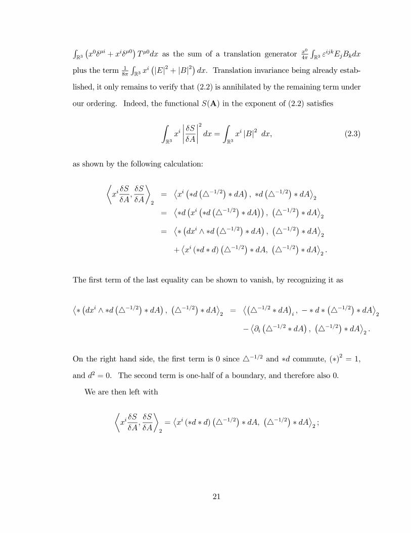
∫R3

(x0δµi + xiδµ0

)T µ0dx as the sum of a translation generator x0

4π

∫R3

εijkEjBkdx

plus the term 18π

∫R3

xi(|E|2 + |B|2

)dx. Translation invariance being already estab-

lished, it only remains to verify that (2.2) is annihilated by the remaining term under

our ordering. Indeed, the functional S(A) in the exponent of (2.2) satisfies

∫

R3

xi

∣∣∣∣δS

δA

∣∣∣∣2

dx =

∫

R3

xi |B|2 dx, (2.3)

as shown by the following calculation:

⟨xi δS

δA,δS

δA

⟩

2

=⟨xi

(∗d

(−1/2

)∗ dA

), ∗d

(−1/2

)∗ dA

⟩2

=⟨∗d

(xi

(∗d

(−1/2

)∗ dA

)),(−1/2

)∗ dA

⟩2

=⟨∗(dxi ∧ ∗d

(−1/2

)∗ dA

),(−1/2

)∗ dA

⟩2

+⟨xi (∗d ∗ d)

(−1/2

)∗ dA,

(−1/2

)∗ dA

⟩2

.

The first term of the last equality can be shown to vanish, by recognizing it as

⟨∗(dxi ∧ ∗d

(−1/2

)∗ dA

),(−1/2

)∗ dA

⟩2

=⟨(−1/2 ∗ dA

)i, − ∗ d ∗

(−1/2

)∗ dA

⟩2

−⟨∂i

(−1/2 ∗ dA

),(−1/2

)∗ dA

⟩2

.

On the right hand side, the first term is 0 since −1/2 and ∗d commute, (∗)2 = 1,

and d2 = 0. The second term is one-half of a boundary, and therefore also 0.

We are then left with

⟨xi δS

δA,δS

δA

⟩

2

=⟨xi (∗d ∗ d)

(−1/2

)∗ dA,

(−1/2

)∗ dA

⟩2

;

21

using the fact that −d ∗ d ∗(−1/2

)∗ dA = 0, we can write

⟨xi (∗d ∗ d)

(−1/2

)∗ dA,

(−1/2

)∗ dA

⟩2

=⟨xi (∗d ∗ d− d ∗ d∗)

(−1/2

)∗ dA,

(−1/2

)∗ dA

⟩2

=⟨xi

(−1/2

)∗ dA,

(−1/2

)∗ dA

⟩2

=⟨xi

(−1/2

)∗ dA,

(−1/2

)∗ dA

⟩2

Using the integral kernel representation of −1/2, and writing Bj for the coordinate

representation of B = ∗dA, we can rewrite the first slot in the inner product:

xi(−1/2B

)= xi 1

2π2

(∫

R3

yBj (y)

|x− y|2d3y

)

=1

2π2

(∫

R3

y (xiBj (y))

|x− y|2d3y

)

= −1/2(xiB

)

This means that

⟨xi

(−1/2

)∗ dA,

(−1/2

)∗ dA

⟩2

=⟨−1/2

(xiB

), −1/2B

⟩2

=⟨xiB, B

⟩2

by self-adjointness of −1/2.

The relation (2.3) allows the extra term 18π

∫R3

xi(|E|2 + |B|2

)dx in the boost

generator to be ordered in the same way as the Hamiltonian, securing boost invari-

ance.

22

Chapter 3

Scalar ϕ4 theory

Adding a ϕ4 interaction term to the free massive scalar field theory considered in

§2.1 results in the classical Lagrangian and Hamiltonian

L (ϕ, ϕ) =

∫

R3

1

2∂µϕ∂

µϕ− m2

2ϕ2 − λ

2ϕ4 dx

H (ϕ, π) =

∫

R3

1

2π2 +

1

2|∇ϕ|2 +

m2

2ϕ2 +

λ

2ϕ4 dx.

In the context of more conventional perturbative quantizations, it is widely expected

that quantized scalar ϕ4 theory will in fact turn out to be free, its interactions being

rendered trivial by a vanishing renormalized coupling constant. In five or more

spacetime dimensions, this has been proven to be the case; in four dimensions there

is no complete proof, but evidence exists [9].

By contrast, a nonlinear normal ordered canonical quantization of scalar ϕ4 theory

results in a ground state distinct from that of the free theory. This is a visible

demonstration of inequivalence between our quantization and the more usual schemes

(recall the discussion of §1.4). Since no fundamental scalar fields have been observed

in nature, we have no basis for any evaluative judgement, and for this reason primarily

23

regard the nonlinear normal ordered quantization of scalar ϕ4 theory as a model

problem for techniques to be used for Yang-Mills theory (Chapter 4), and eventually

in future work general relativity (Chapter 5).

To find the nonlinear normal ordered ground state for scalar ϕ4 theory, we con-

sider the zero-energy imaginary-time Hamilton-Jacobi equation

∫

R3

∣∣∣∣δS

δϕ

∣∣∣∣2

dx =

∫

R3

|∇ϕ|2 + λϕ4 + m2ϕ2 dx. (3.1)

Constructing a solution by the method described in §1.3 requires us to find a min-

imizer ϕt for −∫∞0

L (ϕt, ϕt) dt satisfying the initial data ϕ|t=0 = ϕ. We proceed

to do this using notation and results from Giusti [10], within the “direct method”

for calculus of variations. Another possible approach to the Euclidean Dirichlet

problem for scalar ϕ4 theory has been investigated by H. Lindblad, using existence

results for solutions of partial differential equations given restrictions on the initial

data [22].

3.1 Direct method: General results and tech-

niques

The argument for existence of a minimizer of the functional

F(u) =

∫

U

F (x, u(x), Du(x)) dx

depends on the concept of “minimizing sequences.” For a functional F(u) considered

over functions u belonging to some set V , a minimizing sequence is a sequence uk ⊂

V s.t. limk→∞

F(uk) = infV

F . Clearly by definition of infimum, at least one minimizing

24

sequence must exist. The method of finding a minimizer will be to show that under

suitable conditions, there exists a minimizing sequence which converges (in some

topology) to a limiting function u in V , such that F(u) = infV

F . If we have a function

u = limk→∞

uk in some topology, the key to asserting F(u) = limk→∞

F(uk) = infV

F will be

the property of “lower semicontinuity,” as follows. For the present we will assume

without specification an appropriate topology in which to work; later this issue will

be settled.

Definition 2 A functional is called “lower semicontinuous” on V if for every se-

quence vk ⊂ V , vk → v,

F(v) ≤ limk→∞

inf F(vk).

Thus for a lower semicontinuous functional F on V , a convergent minimizing

sequence uk ⊂ V , uk → u ∈ V in fact yields a minimizer u ∈ V of F , since

infV

F ≤ F(u) ≤ limk→∞

inf F(uk) = infV

F ,

or

F(u) = infV

F .

It only remains, then, to show that in some suitable topology, our functional F is

lower semicontinuous and a convergent minimizing sequence exists. The following

theorem from [10] (Theorem 4.5) gives conditions guaranteeing lower semicontinuity

of F :

Theorem 3 Let U be an open set in Rn, X a closed set in RN , and F (x, u, z) a

25

function defined in U ×X × Rν such that

(i) F is measurable in x ∀ (u, z) ∈ X × Rν; continuous in (u, z)

for almost every x ∈ U

(ii) F (x, u, z) is convex in z for almost every x ∈ U , ∀ u ∈ X

(iii) F ≥ 0.

Suppose

uk, u ∈ L1(U,X), uk → u

zk, z ∈ L1(U,Rν), zk z

in L1loc(U); (*)

Then ∫

U

F (x, u, z) dx ≤ limk→∞

inf

∫

U

F (x, uk, zk) dx.

A proof is given in [10], and will not be repeated here.

To apply this theorem to functionals of the form F(u) =∫UF (x, u,Du) dx,

Rellich’s Theorem (Theorem 3.13 in [10]) can be employed:

Theorem 4 Let Λ be a bounded open set in Rn, with Lipschitz-continuous boundary

∂Λ. Let p, q be such that 1 ≤ p < n, 1 ≤ q < p∗ ≡ npn−p

. Then the immersion1

W 1,p(Λ) → Lq(Λ)

is compact (i.e. continuous and maps bounded sets to relatively compact sets).

The important point is that by Rellich’s Theorem, a sequence uk converging

weakly to u in W 1,ploc (U) must also converge strongly to u in Lp

loc(U). Weak conver-

gence in W 1,ploc (U) is equivalent to weak W 1,p convergence in every open bounded set

1Note that the immersion W 1,p(Λ) → Lp∗

(Λ) is guarateed to exist by the Sobolev imbeddingtheorems, e.g. Thm 3.11 in [10]. Since Λ is bounded, Holder’s inequality shows that Lp

∗

(Λ) ⊂L1(Λ), and from here we can again use Holder’s inequality to show that ∀ r ∈ (1, p∗), Lp∗(Λ) ⊂Lr(Λ) (this is a standard result; see for example [8]).

26

Λ ⊂ U . By the Principle of Uniform Boundedness,‖uk‖1,p,Λ

is bounded, which

implies by Rellich’s Theorem that uk is relatively compact in Lp(Λ) (since p < p∗).

Thus every subsequence of uk has a convergent subsequence, and since uk con-

verges weakly to u in Lp(Λ), all convergent subsequences of uk must converge

strongly to u in Lp(Λ). Therefore uk converges strongly to u in Lploc(U).

This analysis provides the necessary information to verify that the hypotheses of

Theorem 3 are satisfied by a functional of the form F(u) =∫UF (x, u,Du) dx and

a sequence uk weakly convergent to u in W 1,1loc (U,X). Such a sequence converges

strongly to u in L1loc(U,X), as discussed. Meanwhile Duk lies in L1loc(U), and any

functional ω ∈ (L1loc(U))∗

and acting on Dv, v ∈ W 1,1loc (U,X), can be interpreted to

be a functional in(W 1,1

loc (U,X))∗

. Thus weak convergence of uk in W 1,1loc (U,X)

implies weak convergence of Duk in L1loc(U). Taking z in Theorem 3 to be Du

and zk to be Duk, (∗) holds for uk weakly convergent to u in W 1,1loc (U,X). It would

only remain to verify conditions (i), (ii), and (iii) for F .

Before finally applying Theorem 3 to the functional F(u) =∫UF (x, u,Du) dx,

one last observation simplifies the search for a minimizing sequence. Holder’s in-

equality ensures that W 1,ploc (U,X) (p > 1) is a subset of W 1,1

loc (U,M) and that W 1,ploc

convergence implies W 1,1loc convergence and W 1,p

loc weak convergence implies W 1,1loc weak

convergence. This is fortunate, because W 1,ploc has the major advantage over W 1,1

loc of

being a reflexive space. By the Alaoglu Theorem, in a reflexive space every bounded

sequence has a weakly convergent subsequence.

Since a minimizing sequence uk u in W 1,ploc (U,X) will also converge weakly in

W 1,1loc (U,X), such a uk would be sufficient to the matter at hand. On the other

side of the coin, we could also say that lower semicontinuity of a functional F(u) with

respect to the weak topology of W 1,1loc (U,X) implies lower semicontinuity of F(u) with

respect to weak W 1,ploc (U,X), also implying that uk u in W 1,p

loc (U,X) is sufficient.

27

Moreover as remarked above, Alaoglu’s Theorem yields that in fact a minimizing

sequence bounded in W 1,ploc (U,X) would be enough. A simple condition on the

functional F(u) to be “coercive” guarantees that in fact all minimizing sequences

will be bounded:

Definition 5 A functional F(u) on W 1,p(Λ) is called “coercive” if

lim‖u‖1,p→∞

F(u) = +∞.

The result of this analysis is an existence theorem (Theorem 4.6 in [10]) for a

minimizer of F(u):

Theorem 6 If F is lower semicontinuous in the weak topology of W 1,ploc (U,X) and

V is a weakly closed subset of W 1,ploc (U,X) on which F is coercive, then F takes a

minimum in V .

3.2 Application to ϕ4 theory

At last Theorem 6 can be applied to the functional

F (ϕ) = −I (ϕ) =

∫

R+×R3

∣∣(4)∇ϕ∣∣2 + λϕ4 + m2ϕ2 dx dt,

allowing us to find the imaginary-time zero-energy Hamilton-Jacobi functional for

scalar ϕ4 theory. In this ansatz, U is R+ × R3 and X is R. For given initial

data ϕ0, the set V in Theorem 6 is ϕ : ϕ|t=0 = ϕ0. As discussed in §3.7 of [10],

the concept of boundary values (“traces”) for W 1,p(U) functions is meaningful when

suitably defined, and weak W 1,p(U) convergence uk u implies Lploc convergence

of of the traces ψk → ψ on ∂U (subject to conditions on ∂U , which in our case is

28

simply the t = 0 copy of R3 in R+ × R3, and therefore easily satisfies the requisite

smoothness hypotheses). Therefore V is weakly closed, as required. The functional

F is coercive by inspection with respect to W 1,2loc (R+ × R3), and equally easily seen

to be Caratheodory, positive, and convex, verifying that it is lower semicontinuous

in the weak topology of W 1,2loc (R+ × R3). Therefore the desired minimizer exists in

V .

The minimizer we have just found can also be shown to be unique. The following

proof is due to V. Moncrief.

Proposition 7 The minimizer found above for the functional

F (ϕ) =

∫

R+×R3

∣∣(4)∇ϕ∣∣2 + λϕ4 + m2ϕ2 dx dt,

for given initial data ϕ|t=0 = ϕ0, is unique.

Proof. Suppose ϕ1 and ϕ2 are two distinct minimizers for F , for given initial data

ϕ|t=0 = ϕ0. Then both are solutions of the corresponding Euler-Lagrange equation:

−(4)ϕi + m2ϕi + λϕ3i = 0.

Use the parameter τ ∈ [0, 1] to interpolate linearly between ϕ1 and ϕ2:

ϕτ ≡ τϕ1 + (1 − τ)ϕ2,

29

so that dϕτdτ

= ϕ1 − ϕ2. Starting from the Euler-Lagrange equation, we have

0 =

∫ 1

0

d

dτ

[−(4)ϕτ + m2ϕτ + λϕ3τ

]dτ

=

∫ 1

0

−(4) (ϕ1 − ϕ2) + m2 (ϕ1 − ϕ2) + 3λϕ2τ (ϕ1 − ϕ2) dτ

= −(4) (ϕ1 − ϕ2) + m2 (ϕ1 − ϕ2) + 3λ (ϕ1 − ϕ2)

∫ 1

0

ϕ2τ dτ .

Multiplying both sides by (ϕ1 − ϕ2) and integrating over R+ ×R3, we obtain

0 =

∫

R+×R3(ϕ1 − ϕ2)

−(4) (ϕ1 − ϕ2) + m2 (ϕ1 − ϕ2) + 3λ (ϕ1 − ϕ2)

∫ 1

0

ϕ2τ dτ

;

at this point, equality of ϕ1 and ϕ2 at t = 0 and decay of both fields as |x| → ∞

allow us to integrate by parts in the first term of the above integral, yielding

0 =

∫

R+×R3

∣∣(4)∇ (ϕ1 − ϕ2)∣∣2 + m2 (ϕ1 − ϕ2)

2 + 3λ (ϕ1 − ϕ2)2

∫ 1

0

ϕ2τ dτ

.

Since all terms inside the integral are greater than or equal to 0, we must conclude

ϕ1 − ϕ2 = 0.

We can now define our Hamilton-Jacobi functional. This has for its domain

the set of scalar field configurations on R3, interpreted in the Dirichlet problem as

the t = 0 slice of R+ × R3. For notational convenience, we now allow ϕ to denote

field configurations on R3 (rather than R+×R3 as above). Each field configuration

ϕ is the initial value for a guaranteed minimizer ϕt of the functional F , so that

ϕt=0 = ϕ. The imaginary-time zero-energy Hamilton-Jacobi functional S (ϕ) can

30

then be written2

S (ϕ) =

∫

R+×R3

∣∣(4)∇ϕt

∣∣2 + λϕ4t + m2ϕ2t dx dt.

The corresponding zero-energy ground state for the nonlinear normal ordering is

Ω (ϕ) = N exp (−S (ϕ)) .

2Note that for S (ϕ) to be finite, we are implicitly making the assumption that for every set ofinitial data ϕ we are interested in, there exists at least one trajectory ϕs (ϕs=0 = ϕ), for which−∫∞

0L (ϕs, ϕs) dt is finite. This constraint defines the set of physical fields, since for any ϕ on

R3 for which no such ϕs on R+ ×R3 can be found, allowing S (ϕ) to take an infinite value implies

that evaluated on this ϕ, the ground state Ω(ϕ) is zero.

31

Chapter 4

Yang-Mills theory

Yang-Mills theory arose as a generalization of the Maxwell theory of electromag-

netism. While the concept of symmetries constraining the laws of physics has been

central since Galilean relativity, the new and powerful idea in Maxwell theory is

that symmetries can act not only on space and time but on internal spaces in which

the physical fields take their values. Solutions to a physical system are no longer

represented by a single function over spacetime, but by an equivalence class of such

functions related by smoothly varying local symmetries. More physically stated,

a field has local internal degrees of freedom (gauge freedom) on which a structure

group can act, without changing the measurable properties of the field.

In electromagnetism, the structure group is U (1), meaning that gauge symmetry

acts on the potential A by means of a function valued in i ·u(1) (that is, a real-valued

function f). Because U (1) is abelian, the action of the gauge group on A is given

by

A → A + df,

and the field strength F (and electric and magnetic fields E and B) are left unchanged

by gauge transformations. The success of electrodynamics prompted the question

32

of whether other — nonabelian — structure groups could be used to construct gauge

theories representing the remaining fundamental forces of nature. Yang and Mills’s

discovery of nonabelian gauge theories led to the description of the electroweak force

as an SU (2)×U (1) gauge theory (modified by the Higgs mechanism to account for

the mass of weak gauge bosons), and of the strong nuclear force as an SU (3) gauge

theory. However, it is still an open question whether rigorous quantum Yang-Mills

theories exist. In fact, demonstrating a rigorous quantization of pure Yang-Mills

theory in four dimensions for a compact simple gauge group G, and proving that

this theory exhibits a “mass gap” > 0 (i.e., that the Hamiltonian operator has no

eigenvalues in the interval (0,)), is a Clay Prize Millenium Problem (see [17]).

Our primary aim here lies not in the direction of the mass-gap problem (though

of course any progress on rigorously quantized Yang-Mills theory is interesting), but

more generally investigating promising strategies for overcoming hurdles inherent in

quantization of theories with gauge degrees of freedom. In particular, nonabelian

gauge theory is a reasonable testing ground for ideas to be applied to quantum

gravity. After all, the Kodama state arose as a generalization of the Chern-Simons

state from Yang-Mills theory; a first place to look for alternatives to the Kodama

state, then, might be in more well-behaved candidate ground states for Yang-Mills.

In the context of general relativity, no mass gap is expected, and therefore in this

quantization of Yang-Mills theory we do not seek a mass gap, since our goal is a

quantization generalizable to quantum gravity.

In the following sections, we present a nonlinear normal ordered ground state

for Yang-Mills theory with a compact gauge group G ⊂ SO (l). We prove that this

ground state is gauge invariant and invariant under spatial translations and rotations.

Completing the Poincare group, invariance under boosts is conjectured, and remains

as a question for future work.

33

4.1 Mathematical formalism

The main ingredient in a Yang-Mills theory is the structure group; this is a compact

Lie group G with Lie algebra g. For P a principal G-bundle over M , the Yang-Mills

field is a connection A ∈ Λ1P ⊗ g. Given a local section σα : Uα → P for some

neighborhood Uα ⊂ M , the connection 1-form A pulls back to a g-valued 1-form1

Aα = σ∗αA on Uα; the transformation of A on overlapping neighborhoods Uα and Uβ is

given by a transition function ταβ : Uα ∩Uβ → G, defined by σβ (x) = σα (x) ταβ(x):

Aα(x) = ταβ(x)−1dταβ(x) + ταβ(x)−1Aβ (x) ταβ(x), x ∈ Uα ∩ Uβ.

The important quantity for Yang-Mills theory is the curvature F ∈ Λ2P ⊗ g of

the connection A, given by F = dPA + 12

[A,A] where the bracket [·, ·] denotes

the graded commutator on forms, so that [A,A] = 2 (A ∧A) . In terms of a local

section σα : Uα → P , F pulls back to a g-valued 2-form Fα = σ∗αF on Uα, given by

Fα = dMAα + 12

[Aα, Aα], transforming as

Fα(x) = ταβ(x)−1Fβ (x) ταβ (x) , x ∈ Uα ∩ Uβ

for ταβ as given above. In local coordinates, F reduces to

Fµν = ∂µAν − ∂νAµ + [Aµ, Aν]

(here [·, ·] is the ordinary commutator in g).

In order to describe the Yang-Mills action, we use the local expressions of F as a

g-valued 2-form on neighborhoods of M ; however all definitions are gauge-invariant

and therefore do not depend on the particular section used to pull back F .

1For details on Hodge theory of Lie-algebra-valued forms used in this section, see the Appendix.

34

The Yang-Mills action can be conveniently couched in terms of the inner product

for g-valued k-forms on the manifold M :

〈η, θ〉2 =

∫

M

tr (η ∧ ∗θ) , (4.1)

where ∗ denotes the Hodge dual with respect to the metric g on M . We occasionally

also write 〈η, θ〉 for the pointwise inner product 〈η, θ〉 = tr (η ∧ ∗θ). In this notation,

the action is given as

I(A) =1

2

∫

M

tr (F ∧ ∗F ) =1

4

∫

M

trFµνFµν√gdx1 · · · dxn.

Gauge invariance of the form tr (F ∧ ∗F ) negates any ambiguity due to choice of

local trivialization.

The Yang-Mills field equations are

dA ∗ F = 0

where dA = d + [A, ·] is the exterior covariant derivative; solutions of this system

correspond exactly to critical points of the Yang-Mills action I(A). To see this, vary

I(A) by varying A as A + λh, where h vanishes at t = 0 and is supported on some

compact subset N (dependent on h) of M :

δh (I) (A) =

∫

N

〈dAh, F 〉 =

∫

N

tr (dAh ∧ ∗F )

=

∫

∂N

tr (h ∧ ∗F ) −∫

N

tr (h ∧ dA ∗ F ) .

It is evident that δh (I) (A) vanishes for all variations h precisely when dA ∗ F is

identically 0.

35

To make the transformation from a Lagrangian to a Hamiltonian formulation, we

specialize to the case M = R+ × R3. Since M is contractible, every bundle over M

is trivial and therefore admits a global section. We can then drop the distinction

between A and its local coordinate representation.

As in the case of Maxwell theory (§2.3), working in Weyl gauge is necessary for

the Legendre transform to be well-defined. Thus our canonical position variable

is AIi , where i runs over the three spatial parameters and I over the basis of the

Lie algebra g, and the canonical momentum is EiI = AI

i (this is the negative of the

“electric field” variable).

With respect to these variables we obtain the Hamiltonian

H =1

2

∫

R3

tr(E2 + B2

), (4.2)

where Bi = 12εijkFjk. Hamilton’s equations follow by writing the integral J =

∫∞0

H

dt as∫∞0

∫R3

H dx dt = −I +∫∞0

∫R3

EA dx dt. Varying both expressions with

respect to a one-parameter family Aλ (where the variation has compact support in

R+ × R3 and vanishes for t = 0), we arrive at the equality

dJ

dλ=

∫ ∞

0

∫

R3

δH

δAδA +

δH

δEδE

=

∫ ∞

0

∫

R3

[EδA + AδE

]− dI

dλ

=

∫ ∞

0

∫

R3

[−EδA + AδE

]− dI

dλ,

using integration by parts. In order for equality to hold between the first and last

36

lines for all variations, Hamilton’s equations

E = −δH

δA

A =δH

δE

must be equivalent to the vanishing of the variation δIδA

.

4.2 Canonical quantization

The position and momentum variables described in §4.1 are promoted to operators

in a canonically quantized gauge theory. Classically, the Poisson bracket relations

are

AI

i (x) , AJj (y)

= 0 =

Ei

I (x) , EjJ (y)

,

Ej

J (y) , AIi (x)

= δ3 (x, y) δjiδ

IJ .

With the assignment of quantum operators

AIi (x) : ψ(A) → AI

i (x)ψ(A)

EiI(x) : ψ(A) → −i

δ

δAIi (x)

ψ(A),(4.3)

the commutators of mirror the classical Poisson brackets, as required:

[AI

i (x), AJj (y)

]= 0 =

[Ei

I(x), EjJ(y)

],

[Ej

J(y), AIi (x)

]= −iδ3 (x, y) δjiδ

IJ .

where we have set Planck’s constant equal to 1.

In terms of these operators, we search for a quantum ground state for the non-

linear normal ordered Hamiltonian operator. Notice that in taking the Weyl gauge

A0 = 0 in §4.1, we have lost the field equations describing gauge transformations,

37

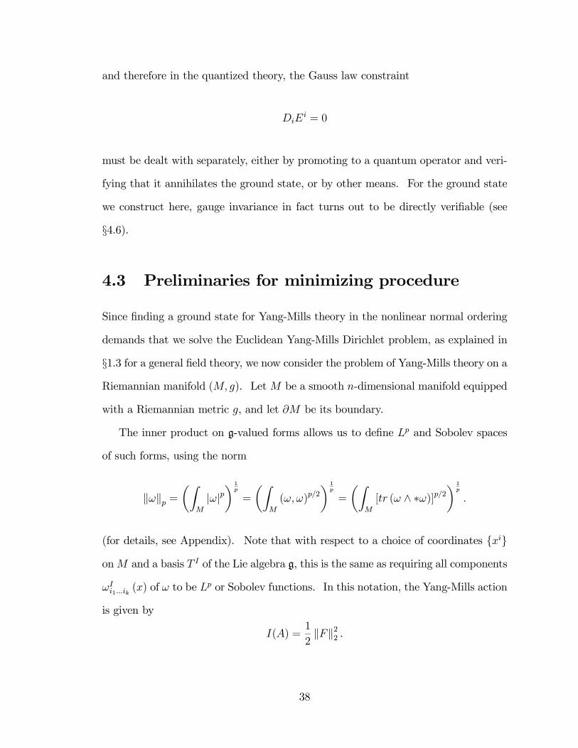
and therefore in the quantized theory, the Gauss law constraint

DiEi = 0

must be dealt with separately, either by promoting to a quantum operator and veri-

fying that it annihilates the ground state, or by other means. For the ground state

we construct here, gauge invariance in fact turns out to be directly verifiable (see

§4.6).

4.3 Preliminaries for minimizing procedure

Since finding a ground state for Yang-Mills theory in the nonlinear normal ordering

demands that we solve the Euclidean Yang-Mills Dirichlet problem, as explained in

§1.3 for a general field theory, we now consider the problem of Yang-Mills theory on a

Riemannian manifold (M, g). Let M be a smooth n-dimensional manifold equipped

with a Riemannian metric g, and let ∂M be its boundary.

The inner product on g-valued forms allows us to define Lp and Sobolev spaces

of such forms, using the norm

‖ω‖p =

(∫

M

|ω|p) 1

p

=

(∫

M

(ω, ω)p/2) 1

p

=

(∫

M

[tr (ω ∧ ∗ω)]p/2) 1

p

.

(for details, see Appendix). Note that with respect to a choice of coordinates xi

on M and a basis T I of the Lie algebra g, this is the same as requiring all components

ωIi1...ik

(x) of ω to be Lp or Sobolev functions. In this notation, the Yang-Mills action

is given by

I(A) =1

2‖F‖22 .

38

To solve the Yang-Mills Dirichlet problem for a compact manifold M , Marini [24]

introduces a terminology for coverings of M by geodesic balls and half-balls; these are

described respectively as neighborhoods of type 1 and type 2. Thus neighborhoods

of type 1, in the manifold’s interior, are denoted

U (1) ≡x =

(x0, ..., xn−1

): |x| < 1

while neighborhoods of type 2, centered around points x ∈ ∂M , are of the form

U (2) ≡x =

(x0, ..., xn−1

): |x| < 1, x0 ≥ 0

,

where the coordinate x0 parametrizes unit-speed geodesics orthogonal to ∂M =

x0 = 0. The boundary of a type 2 neighborhood divides into

∂1U =x ∈ ∂U (2) : x0 = 0

,

∂2U =x ∈ ∂U (2) : |x| = 1

.

In our problem, the manifold of interest is R+ × R3 with the Euclidean met-

ric; however we solve the Yang-Mills Dirichlet problem for a general smooth 4-

dimensional Riemannian manifold with boundary, generalizing Marini’s procedure

to the non-compact case (§4.4). Certain results used are also valid in general dimen-

sion n; such distinctions are clearly noted in the statements. We return to consider

the importance of dimension more thoroughly in §4.4.

To use the direct method for minimizing the Yang-Mills action, we need lower

semicontinuity, as in the Dirichlet problem for scalar ϕ4 theory (Chapter 3).

Theorem 8 The Yang-Mills functional on a manifold M of dimension 4 is lower

semicontinuous with respect to the weak topology on W 1,2loc (M) .

39

Proof. Recalling the definition of lower semicontinuity (Definition 2, Chapter 3),

it is good enough to prove that on any open bounded set U ⊂ M , if Ai A in

W 1,2 (U), then I (A) ≤ lim infi→∞ I (Ai). Locally we can write

Fi = dAi +1

2[Ai, Ai] .

Using the same reasoning as Sedlacek’s in Lemma 3.6 of [32], weak convergence

of Ai to A in W 1,2 (U) implies weak convergence of dAi to dA in L2 (U) . The

continuity of the imbedding W 1,2 → L4 and of the multiplication L4×L4 → L2 along

with boundedness of||Ai||2,1

implies that || [Ai, Ai] ||2 is bounded. This together

with a.e. pointwise convergence yield [Ai, Ai] [A,A], so that Fi F in L2 (U ;P ).

Finally, lower semicontinuity of the ||·||2 norm concludes lower semicontinuity of the

Yang-Mills functional.

4.4 Solving the Yang-Mills Dirichlet problem

For M a compact manifold with boundary ∂M , the Yang-Mills Dirichlet problem

has been collectively solved by Uhlenbeck [37], Sedlacek [32], and Marini [24], using

the direct method in the calculus of variations. The argument begins with a local-

izing theorem, proving that given a sequence of connections with a uniform global

bound on the Yang-Mills action, there exists a cover for M (possibly missing a finite

collection of points) such that on neighborhoods of the cover, the Yang-Mills action

for connections in the sequence eventually becomes lower than an arbitrary pre-set

bound ε. This result depends on compactness as proved in [32] (see Proposition 3.3,

or in [24] Theorem 3.1). We reprove the result here in a manner independent of

compactness (Theorem 10), so that the overall argument now applies to noncompact

40

manifolds with boundary as well.

Note that another possible solution to the problem would be to transform M =

R+×R3 into a compact manifold with boundary, using inversion in the sphere (this

suggestion is due to T. Damour). In this approach, one considers the unit sphere

centered at the origin of R4, imbedding R+×R3 into R4 as the set x : x0 ≥ 2. The

inversion mapping is

yi =xi

r2,

where r2 = (x0)2

+ (x1)2

+ (x2)2

+ (x3)2. Under this transformation, the hyperplane

x0 = 2 maps to a sphere S1/4 of radius 14, with its south pole (the image of all points

at infinity) at the origin. The half-space x : x0 > 2 maps to the interior of S1/4.

Since the mapping is conformal, the Yang-Mills action remains invariant, and the

problem of interest on R+ × R3 has been effectively mapped to a compact problem,

to which the arguments of [37], [32], and [24] should apply directly. We do not

pursue this approach here, since the crucial result using compactness can be shown

to generalize (Theorem 10); however we note its potential usefulness to future work,

such as the investigation of uniqueness of solution to the Yang-Mills Dirichlet problem

(see §4.5). An issue pertinent to the conformal mapping approach is the behavior

of initial data at the south pole of S1/4, the image of points at infinity.

Returning to our sketch of the Yang-Mills Dirichlet problem’s solution, local

control over the Yang-Mills action is used to prove existence and regularity of a

minimizer. From this point on, the proofs in [37], [32], and [24] are purely local and

hold unchanged in the noncompact case; proofs are thus not repeated here. Locally,

the argument for existence of a Yang-Mills minimizer consists in finding a Sobolev-

bounded minimizing sequence satisfying the boundary conditions; this sequence then

has a weakly convergent subsequence, which proves to be a solution to the original

41

Dirichlet problem. Local solutions are related by transition functions on overlapping

neighborhoods.

Gauge freedom turns out to be a help as well as a hindrance. Of course it

forces the necessity of working locally and proving compatibility on overlaps, but at

the same time gauge freedom offers an elegant solution to the regularity problem.

A judicious choice of gauge — the “Hodge gauge” — complements the Yang-Mills

equation in such a way as to yield an elliptic system. In the Yang-Mills equation

d ∗ dA + [A, dA] + [A, [A,A]] ,

the highest order term is related to the first term of the Laplace-de Rham operator

∆ = δd+dδ, where δ is the codifferential δ = (−1)n(k+1)+1 ∗d∗ (k being the degree of

the differential form operated upon). Choosing the Hodge gauge, in which d∗A = 0,

ensures that every solution of our system in this gauge is also a solution of the

elliptic system ∆A+ ∗ ([A, dA] + [A, [A,A]]) = 0, and therefore enjoys the regularity

properties of such solutions. (Additional work is needed to establish boundary

regularity; Marini accomplishes this in [24] using the technique of local doubling.)

In the physical problem, we are interested in Yang-Mills theory over a 4-dimensional

manifold with boundary. However many theorems which follow are also valid over

any smooth n-dimensional Riemannian manifold with boundary, and we retain this

level of generality in stating and proving results. The caveat lies in stringing together

the individual theorems into a complete argument for existence and regularity of a

solution to the Yang-Mills Dirichlet problem; to accomplish this, the dimension must

be 4 (see the remarks in [24] following Theorem 3.1). The “good cover” theorem

(Theorem 10 here, or Theorem 3.1 in [24]) guarantees a cover of M\ x1, ..., xk on

whose neighborhoods the local Yang-Mills action for the connections in the sequence

42

is eventually bounded by an arbitrary pre-set bound ε. However, the condition for

existence of a Hodge gauge solution to the Yang-Mills Dirichlet problem is a bound

on the local Ln/2 norm of the Yang-Mills field strength F , which except in dimension

4 is not the same as a local bound on the Yang-Mills action.

Without further ado, we give the precise statements of all theorems needed for the

existence and regularity of a Yang-Mills minimizer on a 4-dimensional manifold with

boundary. On a neighborhood U of type 1 or 2, the condition for local existence of

a gauge satisfying d∗A = 0 is an Ln/2 bound on Yang-Mills field strength. Consider

the sets

A1,pK (U) =

D = d + A : A ∈ W 1,p(U), ‖FA‖Ln/2(U) < K

B1,pK (U) =

D = d + A :

A ∈ W 1,p(U)

Aτ ∈ W 1,p(∂1U),

‖FA‖n/2 < K

‖FAτ‖Ln/2(∂1U) < K

describing connections with field strength locally Ln/2-bounded on a neighborhood

U of type 1 and type 2, respectively. (All norms are defined on U , unless otherwise

specified.) As proven in [37] (Theorem 2.1) for interior neighborhoods and in [24]

(Theorems 3.2 and 3.3) for boundary neighborhoods, a good choice of gauge exists

for connections belonging to A1,pK (U) or B1,pK (U). More precisely,

Theorem 9 For n2≤ p < n, there exists K ≡ K(n) > 0 and c ≡ c(n) such that

every connection D = d+A ∈ A1,pK (B1,pK ) is gauge equivalent to a connection d+ A,

43

A ∈ W 1,p(U), satisfying

(a) d ∗ A = 0 (a′)

d ∗ A = 0

dτ ∗ Aτ = 0 on ∂1U

(b) Aν = 0 on ∂U (b′) Aν = 0 on ∂2U

(c = c′)∥∥∥A

∥∥∥1,n/2

< c(n) ‖FA‖n/2

(d = d′)∥∥∥A

∥∥∥1,p

< c(n) ‖FA‖p

(Unprimed conditions (a)-(d) refer to A1,pK (U); primed conditions (a′)-(d′) toB1,pK (U)).

Moreover, the gauge transformation s satisfying A = s−1ds + s−1As can be taken in

W 2,n/2(U) (s will in fact always be one degree smoother than A; see Lemma 1.2 in

[37]).

Proof. See [37],[24].

As noted in [24], the condition ‖FA‖n/2 < K is conformally invariant, while by

contrast the norm ‖FAτ‖Ln/2(∂1U) picks up a factor of r under the dilation x′ =

rx, so that the simultaneous conditions ‖FA‖n/2 < K, ‖FAτ‖Ln/2(∂1U) < K on a

neighborhood U of type 2 can always be achieved by applying an appropriate dilation

(the Dirichlet boundary data is prescribed to be smooth, so ‖FAτ‖Ln/2(∂1U) already

satisfies some bound).

To find a regular minimizer of the Yang-Mills action on a 4-dimensional manifold

M , we must find a cover Uα of M and a minimizing sequence Ai whose members

satisfy

SYM(Ai|Uα) =

∫

Uα

|FAi|2 dx < K ∀ α, i,

where K ≡ K(4) is as given in Theorem 9. For a compact manifold this is proved

in [32] using a counting argument. Here we use dilations of the neighborhoods in a

44

cover to construct a proof valid for any smooth Riemannian manifold.

Theorem 10 Let A(i) be a sequence of connections in G-bundles Pi over M ,

with uniformly bounded action∫M|F (i)|2 dx < B ∀ i. For any ε > 0, there

exists a countable collection Uα of neighborhoods of type 1 and 2, a collection of

indices Iα, a subsequence A(i)I′ ⊂ A(i)I and at most a finite number of points

x1, ..., xk ∈ M such that

⋃Uα ⊃ M\ x1, ..., xk

∫

Uα

|F (i)|2 dx < ε ∀ i ∈ I ′, i > Iα.

Proof. For each n ∈ N, consider the cover Bn(x) : x ∈ M of M given by geodesic

balls of radius 1n

centered at each point x ∈ M (for x ∈ ∂M , the geodesic “ball”

Bn(x) will actually be a half-ball, a fact which makes no difference in the proof). By

separability, each such cover has a countable subcover Cn = Bn(xn,m) : m ∈ N.

On any ball Bn(xn,m), we have the uniform bound∫Bn(xn,m)

|F (i)|2 dx < B ∀

i. Therefore for the ball Bn(xn,1) in a given cover Cn, there exists a subsequence of

A(i) for which the corresponding subsequence of∫

Bn(xn,1)|F (i)|2 dx

converges.

Of this subsequence, there exists a further subsequence such that the corresponding

subsequence of∫

Bn(xn,2)|F (i)|2 dx

converges, and so on, for every m. Diagonal-

izing2 over these nested subsequences, we obtain a subsequence of A(i) such that

the corresponding subsequence of∫

Bn(xn,m)|F (i)|2 dx

converges for every m ∈ N.

Performing a similar diagonalization over all covers Cn, there exists a subse-

2Diagonalizing over a list of sequences aj (i) such as

a1 (1) a1 (2) a1 (3) . . .

a2 (1) a2 (2) a2 (3) . . .

a3 (1) a3 (2) a3 (3) . . ....

......

. . .

selects out

the new sequence ai (i). In the case important for this proof, each row represents a subsequenceof the previous row, so that for any j, the diagonalized sequence ak (k)is a subsequence of aj (i)for k ≥ j.

45

quence A(i)I′ ⊂ A(i)I such that for every ball in every cover, the sequence∫

Bn(xn,m)|F (i)|2 dx

I′

converges. For each Cn, consider the collection of balls

Bn(yn,m), yn,m ⊂ xn,m, for which∫

Bn(yn,m)|F (i)|2 dx

I′

converges to a value

greater than or equal to ε. Note that for any i ∈ I, there is an upper bound on the

number Ni,n of disjoint balls of radius 1n

for which∫Bn(yn,m)

|F (i)|2 dx ≥ ε :

B ≥ Ni,nε.

Thus the upper bound Bε

limits the number of disjoint balls in the set Bn(yn,m) .

Choose a maximal disjoint setBn(yn,mj

)J

j=1of balls in Bn(yn,m), and consider

the setB∗

n(yn,mj)J

j=1of balls centered at the points yn,mj

but having radius 3n. Then

we have⋃yn,m

Bn(yn,m) ⊂ ⋃Jj=1B

∗n(yn,mj

). This shows that if we discard the balls

Bn(yn,m) from the cover Cn, we will only have discarded a set which was contained

in J ≤ Bε

balls of radius 3n. We can then safely discard the balls Bn(yn,m) from

each cover Cn, and form the union C =⋃

n∈NCn\ Bn(yn,m) to obtain a cover C of

M\ x1, ..., xk, where k ≤ Bε, and each ball Bn (xn,m) ∈ C satisfies

∫Bn(xn,m)

|F |2 < ε.

Since a minimizing sequence A(i)i∈I by definition admits a uniform bound

on the action, we can use Theorem 10 to select a subsequence A(i)i∈I′ of the

minimizing sequence and a cover Uα satisfying∫Uα

|F (i)|2 dx < K(4) ∀ i ∈ I ′,

i > Iα. On any neighborhood Uα in the cover, Theorem 9 implies that each member

Aα(i) of the subsequence is gauge-equivalent to a connection Aα(i) in the Hodge

gauge, satisfying a uniform W 1,2(U) bound on Aα(i). Weak compactness of Sobolev

spaces now yields a further subsequence ofAα(i)

, weakly convergent in W 1,2 to

some Aα. It only remains to show that Aα retains the desired regularity properties

and boundary data, and that the setAα

can be patched to a global connection on

46

M. These objectives are accomplished by Theorem 3.4 in [24] (generalizing Theorem

3.6 in [37] and Theorem 3.1 in [32]). Their results are paraphrased below; the proof

is by weak compactness of Sobolev spaces:

Theorem 11 Let A(i)i∈I be a sequence of G-connections with uniformly bounded

action as described in Theorem 10, and with prescribed smooth tangential boundary

components (A (i))τ = aτ on ∂M . Let ε = K(4), where K(4) is the constant

from Theorem 9. Then, for the subsequence A (i)i∈I′ found in Theorem 10 and

cover Uα, there exists a further subsequence A (i)i∈I′′, sections σα (i) : Uα → Pi

(i ∈ I ′′) and connections Aa on Uα such that

(e) σ∗α (i) (Ai) ≡ Aα (i) Aα in W 1,2 (Uα)

(f) F (Aα (i)) ≡ Fα (i) Fα in L2 (Uα)

(g) sαβ (i) sαβ in W 2,2 (Uα ∩ Uβ)

(h) (Aα)τ |∂1Uα ∼ aτ |∂1Uα by a smooth gauge transformation

(i)

d ∗ Aα = 0 on Uα

dτ ∗ (Aα)τ = 0 on ∂1U

(j) Aα ≡ s−1αβAβsαβ + s−1αβdsαβ

Here sαβ(i) is the transition function Aβ (i) → Aα (i); i.e,

Aα (i) ≡ s−1αβ (i)Aβ (i) sαβ (i) + s−1αβ (i) dsαβ (i) .

Proof. See [32], [24]. Note that the result follows by weak compactness of Sobolev

spaces, after applying diagonalization (as in the proof of Theorem 10) over the count-

able cover Uα.

Lower semicontinuity of the Yang-Mills functional now implies that the value of

the action on the limiting connection A of the sequence described in Theorem 11 is

47

in fact m (aτ ) ≡ minA

I (A) where A is the set of connections on G-bundles on M such

that Aτ |∂M = aτ . In Theorem 3.5 in [24] and 4.1 in [32], it is proved by contradiction

that A in fact satisfies the Yang-Mills equations. These proofs are completely local,

and hold unchanged in our case.

The proofs of regularity of the connection in Hodge gauge are also local and hold

unchanged. Regularity except for at the points x1, ..., xk from Theorem 10 is a

consequence of the ellipticity of the Yang-Mills equations in Hodge gauge (Theorem

4.5, [24]). At the points x1, ..., xk, the limiting connection may not be defined, so

removable singularity theorems are needed to extend A to these points. The case of

interior points is covered by Theorem 4.1 in [38], and by Theorem 4.6 in [24], so that

the connection A extends to a smooth connection (provided the Dirichlet boundary

data is smooth). More precisely, we have

Theorem 12 Let U (1) (U (2)) be a neighborhood of type 1 (2); let U(i)∗ = U (i)\ 0.

Let A be a connection in a bundle P over U(i)∗ , ‖FA‖L2(U) < B < ∞. Then

(Type 1) If A is Yang-Mills on P |U (1)∗ , there exists a C∞ connection A0

defined on U (1) such that A0 is gauge-equivalent to A on U(1)∗ .

(Type 2) If A is Yang-Mills and C∞ on P |U (2)∗ , there exists a C∞ connection A0

defined on U (2) such that A0 is gauge-equivalent to A on U(2)∗ ,

by a gauge transformation in C∞ (U∗).

Proof. See [38], [24].

48

4.5 The Euclidean Yang-Mills Hamilton-Jacobi func-

tional

Having shown the existence of an absolute minimizer At for the Euclidean Yang-Mills

action given prescribed smooth initial tangential components A = aτ , we can now

define the Hamilton-Jacobi functional3

S (A) =

∫

R+×R3tr (FAt ∧ ∗FAt) dt,

where ∗ indicates the Hodge star operator in the Euclidean metric.

The values of this functional are well-defined even allowing for the possible ex-

istence of more than one gauge-equivalence class of minimizers for the given initial

data; in principle we can simply choose a minimizer starting from the field config-

uration A = aτ . However, while still an open question, there exist partial results

toward establishing uniqueness of a minimizer for given initial data in the compact

case. In [13], Isobe has shown that for flat boundary values, the Dirichlet problem on

a star-shaped bounded domain in Rn can only have a flat solution. Non-uniqueness

results are proven by Isobe and Marini [14] for Yang-Mills connections in bundles over

B4, but the solutions are topologically distinct, belonging to differing Chern classes.

On the domain M = R+ × R3, it seems likely that given initial data determines a

minimizer unique up to gauge transformation.

In order to make the claim that S(A) solves the imaginary-time zero-energy Yang-

Mills Hamilton-Jacobi equation, we must also verify its functional differentiability.

This can be done using the same integration by parts argument as in the derivation

of the Euler-Lagrange equation. However, we must first write the solution to the

3Again, we are implicitly assuming that for all initial data A of physical interest, there exists atleast one trajectory As (As=0 = A) such that −I (As) <∞. See the footnote at the end of §3.2.

49

Euclidean Dirichlet problem in a global gauge which is smooth and decays sufficiently

rapidly at spatial and temporal infinity.

First, Theorem 12 implies that the solution A to the Yang-Mills Dirichlet problem

extends to a smooth connection on a smooth bundle over all of M = R+×R3. Since

the only bundle over a contractible base manifold is the trivial one (see e.g. [27]), A

is also a connection on the trivial bundle P ∼= M ×G. Therefore we can write A in

terms of a smooth global section σ : M → G. Using this trivialization, D = d + A

is smoothly defined over all of M .

The following lemma controls the growth of A and F, for a good choice of gauge.

Part (a) is a version of Uhlenbeck’s Corollary 4.2 [38] for our base manifold M =

R+×R3; part (b) extends the same principle to bound the growth of the connection

1-form A.

Lemma 13 Let D = d + A be a connection in a bundle P over an exterior region

V =y ∈ R+ ×R3 : |y| > N

satisfying

∫V|F |2 < ∞. Then

(a) |F | ≤ C |y|−4 for some constant C (not uniform);

(b) There exists a gauge in which D = d + A satisfies∣∣∣A

∣∣∣ ≤ K |y|−2.

Proof. (a) Following the reasoning in [38], we define the conformal mapping

f : U∗ → V

y = f (x) = N x|x|2

,

where U∗ =x ∈ R+ × R3 : 0 < |x| ≤ 1

. By conformal invariance of the Yang-Mills

action, we have ∫

U∗

|f∗F |2 =

∫

U∗

|F (f ∗D)|2 =

∫

V

|F |2 .

Applying part (b) of Theorem 12 to the pullback f∗D of D under f , there exists a

50

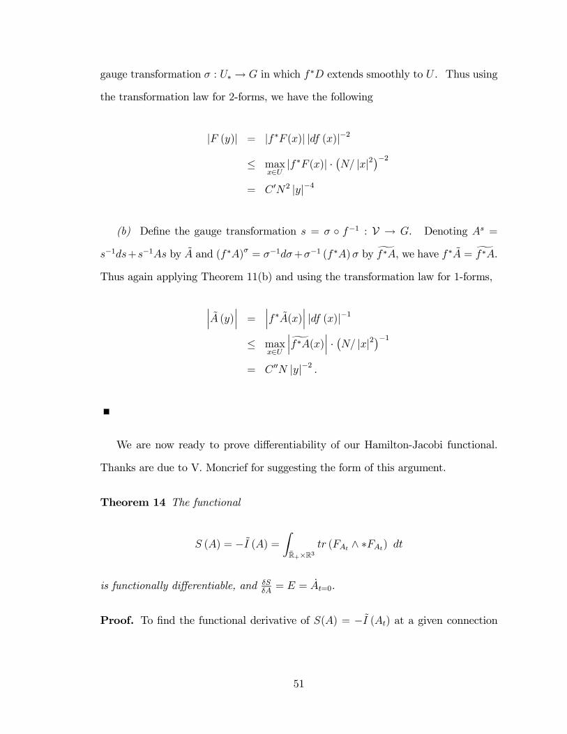
gauge transformation σ : U∗ → G in which f ∗D extends smoothly to U . Thus using

the transformation law for 2-forms, we have the following

|F (y)| = |f ∗F (x)| |df (x)|−2

≤ maxx∈U

|f ∗F (x)| ·(N/ |x|2

)−2

= C ′N2 |y|−4

(b) Define the gauge transformation s = σ f−1 : V → G. Denoting As =

s−1ds+s−1As by A and (f ∗A)σ = σ−1dσ+σ−1 (f ∗A)σ by f ∗A, we have f ∗A = f∗A.

Thus again applying Theorem 11(b) and using the transformation law for 1-forms,

∣∣∣A (y)∣∣∣ =

∣∣∣f ∗A(x)∣∣∣ |df (x)|−1

≤ maxx∈U

∣∣∣f ∗A(x)∣∣∣ ·

(N/ |x|2

)−1

= C ′′N |y|−2 .

We are now ready to prove differentiability of our Hamilton-Jacobi functional.

Thanks are due to V. Moncrief for suggesting the form of this argument.

Theorem 14 The functional

S (A) = −I (A) =

∫

R+×R3tr (FAt ∧ ∗FAt) dt

is functionally differentiable, and δSδA

= E = At=0.

Proof. To find the functional derivative of S(A) = −I (At) at a given connection

51

A0 on the slice x0 = 0, consider the 1-parameter family A0 + λh, constructing

d

dλ[S (A0 + λh)]

∣∣∣∣λ=0

= limλ→0

S (Aλ) − S(A0)

λ

= limλ→0

−I (Aλ,t) −(−I(A0,t)

)

λ

= − limλ→0

1

λ

[I (Aλ,t) − I(A0,t)

]

where for each Aλ = A0+λh, Aλ,t denotes the absolute minimizer of −I given initial

data Aλ. For any given value λ0, the difference I (Aλ0,t) − I(A0,t) can be expressed

in terms of a Taylor series, as follows. First, use the parameter λ to interpolate

between A0,t and Aλ0,t, describing a 1-parameter family Xλ,t,

Xλ,t ≡λ

λ0Aλ0,t +

(1 − λ

λ0

)A0,t,

so that Xλ,0 = Aλ. The standard Taylor series expansion of I (Xλ,t) as a function

of λ then gives

I (Aλ0,t) − I(A0,t) = λ0

(∂I

∂λ

)

λ=0

+ O(λ20

). (4.4)

Let ht = 1λ0

(Aλ0,t − A0,t), so that Xλ,t = A0,t + λht. Then

∂I

∂λ

∣∣∣∣∣λ=0

=∂

∂λ

[∫

R+×R3

⟨FXλ,t

, FXλ,t

⟩]∣∣∣∣λ=0

= 2

∫

R+×R3

⟨dht + [A0,t, ht] , FA0,t

⟩

= 2 limR→∞

(∫

∂1

〈h, FA0〉 +

∫

∂2

⟨ht, FA0,t

⟩−

∫

0≤|x|<R

⟨ht, D

∗FA0,t

⟩)

where ∂1 = |x| < R,x0 = 0 , ∂2 = |x| = R, x0 > 0.

The last term on the right-hand side vanishes due to the fact that FA0,t is a

solution to the Yang-Mills equations. Working with Aλ0,t and A0,t both in the

52

gauge guaranteed by Lemma 13 (for some fixed N which R eventually surpasses),

the middle term also approaches zero as R approaches infinity, since

⟨ht, FA0,t

⟩≤ |ht|

∣∣FA0,t

∣∣

≤ 1

λ0(|Aλ0,t| + |A0,t|)

∣∣FA0,t

∣∣

≤ 1

λ0(Kλ0 + K0)C0 ·R−6.

Since the area element on ∂2 contributes only a factor of R2, the middle term is easily

seen to vanish. Thus we are left with only the first term, so that

∂I

∂λ

∣∣∣∣∣λ=0

=

∫

R3

〈h, FA0〉 ,

and the definition of functional derivative implies that

δS

δA= E = At=0.

4.6 Gauge and Poincare invariance

In order for the candidate ground state wave functional

Ω(A) = N exp (−S (A))

53

to be physical, it must remain invariant under the action of gauge transformations

g (x), x ∈ R3, on the connection A(x) :

S(g−1dg + g−1Ag

)= S (A) ,

so that S is in fact a functional on the physical configuration space A/G of connections

modulo gauge transformations, rather than the kinematical configuration space A.

Gauge invariance of S follows immediately from its form

S(A) = −∫ ∞

0

L(At, At

)dt =

∫

R+×R3tr (FAt ∧ ∗FAt)

where ∗ denotes the Hodge star operator in the Euclidean metric on R+ ×R3. The

gauge transformation g (x), x ∈ R3 can simply be extended to R+ × R3 by taking

g (t, x) = g (x) constant over R+, and the cyclic property of the trace implies

S(g−1dg + g−1Ag

)=

∫

R+×R3tr (Fg·At ∧ ∗Fg·At)

=

∫

R+×R3tr (FAt ∧ ∗FAt) = S (A) .

Similarly, rotations and translations applied to R3 do not affect the value of

S (A), because we can extend them constantly through time over R+×R3, and by a

change of coordinates the value of the integral defining S (A) is unchanged. The only

remaining Poincare transformations are boosts, which cannot be verified directly in

our canonical framework. The conserved quantity generating an infinitesimal boost

in the xi direction is

CB(i) =

∫

R3

(x0δµi + xiδµ0

)T µ0 dx, (4.5)

54

where T µν = − 14π

F µ

αFνα − 1

4ηµνFαβF

αβ

is the stress-energy tensor of Yang-Mills

theory. This constraint must be promoted to a quantum operator which annihilates

our candidate ground state. A test case in which this can be done is the abelian

case of U (1) gauge theory (see §2.3) Using the abelian case as a model, we hope to

extend invariance under boosts to the nonabelian case in future work.

55

Chapter 5

Future work

Immediate plans for future work center around the question of invariance under

boosts of the nonlinear normal ordered ground state for Yang-Mills theory. In

the abelian case, we have verified invariance under boosts as described in §2.3; the

nonabelian case remains.

Additionally, uniqueness of the solution to the Euclidean Yang-Mills Dirichlet

problem is still an open question, and one which it would be desirable to settle.

Gauge freedom renders this problem more difficult to address than, for example, in

the case of scalar ϕ4 theory; however in the compact case, partial uniqueness results

have been established by Isobe and Marini [14], and Isobe [13]. Using a conformal

transformation to map the problem to the compact case, as described in §4.4, is a

possible means of approach.

Beyond these questions filling out the current framework, there are several direc-

tions in which the program can be extended. Most important are its application

to coupled Yang-Mills-Higgs theory, and to general relativity. Another sideline con-

cerns the possibility of defining a non-Gaussian measure from the ground state found

in Chapter 3 for scalar ϕ4 theory.

56

5.1 Yang-Mills-Higgs theory

In the nonabelian Higgs model, the Yang-Mills connection A is coupled to a g-valued

scalar field ϕ. We follow notation of Jaffe and Taubes in [16]. The Lagrangian

action is given by

I =1

4

∫ ∞

0

∫

R3

trFµνF

µν + (dAϕ)µ (dAϕ)µ + λ(|ϕ|2 − 1

)2dx dt.

Canonically, the “position” variables are ϕ,A.

In performing a Legendre transformation, we will again encounter the problem

of indefiniteness due to gauge freedom. In [31], Salmela discusses resolutions of this

issue by gauge-fixing, examining various methods of subsequently implementing the

Gauss constraint. This work will likely prove valuable to our project.

In order to construct a nonlinear normal ordered ground state for Yang-Mills-

Higgs theory, we need to solve the Euclidean Dirichlet problem. Work on regularity

properties of solutions to the Yang-Mills-Higgs system has been done by Parker [29]

and Otway [28].

5.2 General relativity

In presenting the action for general relativity, we follow Smolin’s notation in [34].

The structure group for general relativity is SU (2); we denote by σI3I=1 a basis

of the Lie algebra su(2). Capital Latin indices run over this basis, while lowercase

letters index the three spatial parameters on each spacelike slice Σ of the spacetime

manifold M , assumed to be of the form R × Σ. The “position” in the Ashtekar-

variables framework is an SU (2) connection AIi on Σ; its conjugate momentum is a

57

densitized inverse triad EiI , related to the spacelike metric qij on Σ by

det (q) qij = EiIEjI .

In terms of these variables, the Lagrangian action for general relativity is given by

I =

∫ ∞

0

∫

Σ

EiIAiI −NH−N iHi − wIGI

dx dt.

Each term after the first is a constraint term:

GI = DiEiI = 0

Hi = EjIF

Iij = 0

H = εIJKEiIE

jJ

(FijK − Λ

6εijkE

kK

)= 0,

where Λ is the cosmological constant and as before, F is the curvature of A, given

in coordinates by

F Iij = ∂iA

Ij − ∂jA

Ii + [Ai, Aj ]

I

Just as in Yang-Mills theory, the Gauss law constraint wIGI generates an infinites-

imal gauge transformation given by wI (x) σI . The Hamiltonian constraint NH gen-

erates time evolution, and N iHi generates infinitesimal diffeomorphisms. It is here

that we encounter the largest difference between Yang-Mills theory and general rela-

tivity: where Yang-Mills theory only requires invariance under the Poincare group,

a finite-dimensional subgroup of the diffeomorphism group, general relativity must

respect full diffeomorphism invariance. We thus have infinitely many constraints

to promote to quantum operators, which will undoubtedly render the problem of

factor-ordering the quantum constraints much more difficult.

58

On the other hand, encouragement for the goal of constructing a nonlinear normal

ordered ground state for general relativity comes from Moncrief and Ryan’s explicit

solution in the case of vacuum Bianchi IX cosmology (see [26]). Another starting

point for investigations on a ground state for quantum gravity is Kuchar’s ground

state for linearized gravity [21]

Ω (h) = N exp

− 1

8π2

∫

R3

∫

R3

(hTTik,l(x)

)·(hTTik,l(y)

)

|x− y|2dx dy

,

in terms of the linearized metric tensor

hik = gik − ηik

in vacuum gauge (denoted hTTik ). Strong analogy between this functional and

Wheeler’s ground state for free Maxwell theory (cf. §2.3) is manifest.

A caveat for the Ashtekar variables is the fact that certain versions of the for-

malism (e.g. the original presentation of Sen [33], Ashtekar [1]) require the basic

variables to take complex values. In fact, the usual construction of the Kodama

state necessitates complexifying in order to obtain nontrivial connections A satisfy-

ing the self-dual condition

Fijc −Λ

6εijkE

kc = 0.

This condition leads to the Hamilton-Jacobi equation

Fijc +Λ

6εijk

δS(A)

δAck

= 0,

satisfied by the Chern-Simons functional SCS as given in (1.1); thus exp (SCS (A))

is annihilated by the self-dual condition when promoted to a quantum operator.

59

Working with complex fields, however, is physically undesirable.

5.3 Scalar ϕ4 non-Gaussian measure

In Chapter 3 we obtained the ground state

Ω (ϕ) = N exp

−∫

R+×R3

∣∣(4)∇ϕt

∣∣2 + λϕ4t + m2ϕ2t dx dt

for scalar ϕ4 theory (where as before, ϕt is a minimizer of −I(ϕ) for the initial data

ϕt=0 = ϕ(x)). The natural next question is whether we can use Ω (ϕ) to define a

non-Gaussian measure of the form

dµ(ϕ) = Ω2 (ϕ) dϕ.

Denoting the free scalar field ground state by

Ω0 (ϕ) = N0 exp

−∫

R+×R3

∣∣(4)∇ϕt

∣∣2 + m2ϕ2t dx dt

= N0 exp

−⟨ϕ,H1/2ϕ

⟩2

2

,

we can regard the interacting ground state Ω (ϕ) as a perturbation of Ω0 (ϕ) by the

term O(ϕ) =∫R+×R3

λϕ4tdxdt. From §2.2 we know that Ω0 (ϕ) indeed determines a

Gaussian measure on S ′ (R3).

Since ϕt is determined by ϕ, and moreover its decay is controlled by the fact that it

must minimize −I(ϕ), the time dependence on the right-hand side of O(ϕ) integrates

out. It thus seems possible that this perturbation might be usefully estimated in

terms of the perturbation∫R3

λϕ4dx from the 3-dimensional Euclidean path-integral

approach. Techniques such as those used in [7] might then be employed to define a

60

non-Gaussian measure for our situation.

In the path-integral formalism, functional measures for scalar ϕ4 theory have only

been shown to exist for three spacetime dimensions, as in [7]; a rigorous measure for

scalar ϕ4 path-integrals in four spacetime dimensions has so far eluded definition.

Canonically, however, the full four-dimensional spacetime theory is described by

integration over field configurations on the three-dimensional spatial slice; hence one

fewer dimension is necessary to recover the full theory than in the path-integral

approach. Thus existing results from ϕ43 path integral theory may possibly be

relevant to the full theory here.

61

Appendix

Collected here are a few results and definitions used in this thesis. Throughout, we

follow notation of Baez and Muniain [5], Nakahara [27], and Westenholz [40].

Hodge theory

Real-valued differential forms: The following material is completely stan-

dard, and is recorded here for reference within the thesis, as well as for comparison

with the definitions given below of similar objects in the theory of g-valued differ-

ential forms. For full details, see [5] or [40]. We follow a similar notation to these

authors.

We denote the space of differential k-forms on the manifold M as Λk (M). The

set of all differential forms Λ (M) = ⊕kΛk (M) can be thought of as the algebra

generated by Λ1 (M) with the relation ω ∧ µ = −µ ∧ ω. For higher-order forms

ω ∈ Λk (M) and µ ∈ Λl (M), we have

ω ∧ µ = (−1)kl µ ∧ ω.

A Riemannian metric g on the manifold M allows us to define the Hodge star operator

∗ : Λk (M) → Λn−k (M) . For a positively oriented orthonormal basis of 1-forms

62

e1, ..., en,

∗(ei1 ∧ · · · ∧ eik

)= εi1,...,in

(eik+1 ∧ · · · ∧ ein

);

extend linearly from this definition to the whole of Λk (M). The Hodge star operator

satisfies (∗)2 = (−1)k(n−k).

From the Hodge star operator, we can in turn define an L2 inner product on the

space of k-forms:

〈ω, µ〉2 =

∫

M

ω ∧ ∗µ. (5.1)

The other basic operator on Λ (M) is the exterior derivative d : Λk (M) →

Λk+1 (M), defined as the set of linear maps satisfying

(i) d (ω ∧ µ) = dω ∧ µ + (−1)p ω ∧ dµ, for ω ∈ Λp (M) and µ ∈ Λ (M) .

(ii) d (dω) = 0 for all ω ∈ Λ (M) ,

and such that d : Λ0 (M) → Λ1 (M) on real-valued functions is the 1-form defined

by df (v) = v (f) = vµ ∂f∂xµ

.

With respect to the inner product (5.1), the exterior derivative has an adjoint,

the codifferential, given as

δ ≡ d∗ = (−1)n(k+1)+1 ∗ d∗ (5.2)

when applied to k-forms. The expression in terms of d follows from Stokes’ Theorem.

Just as the exterior derivative extends the gradient operator on functions to all of

Λ (M), the Laplace-de Rham operator, defined as

= dδ + δd,

63

extends the ordinary Laplacian1. In terms of (5.2), we can write

= (−1)nk+1 ((−1)n d ∗ d ∗ + ∗ d ∗ d)

for the Laplace-de Rham operator on k-forms.

g-valued differential forms: Most of the preceding section’s definitions can

be extended to apply not only to real-valued differential forms, but to forms taking

values in the Lie algebra g. Again we follow the presentation of [5], [27], and [39].

For a manifold M , the g-valued k-forms are members of ΛkM⊗g. Denote by ΛM⊗g

the entire space ⊕k

(ΛkM ⊗ g

). Every g-valued k-form can be written as the sum

of terms of the form ω ⊗ S, for ω ∈ Λk (M), S ∈ g. The Hodge dual generalizes to

∗ (ω ⊗ S) = ∗ω ⊗ S,

and we can similarly define the wedge product of g-valued differential forms by

extending linearly from the basic definition

(ω ⊗ S) ∧ (µ⊗ T ) = (ω ∧ µ) ⊗ ST.

These two notions give us the necessary background for introducing the inner product

of g-valued k-forms η and θ:

〈η, θ〉2 =

∫

M

tr (η ∧ ∗θ) .

Note that in the wedge product above, the values from g are combined using the

1More accurately, the Laplace-de Rham operator extends the negative Laplacian −f = − ∂2f∂2x0

−. . .− ∂2f

∂2xn, a convention adopted because − has nonnegative eigenvalues.

64

product operation, but also important is their Lie bracket. For two g-valued forms

η = (ω ⊗ S) ∈ ΛkM ⊗ g and θ = (µ⊗ T ) ∈ ΛlM ⊗ g, we can use their Lie bracket

to form the graded commutator

[η, θ] ≡ η ∧ θ − (−1)kl θ ∧ η

= (ω ∧ µ) ⊗ [S, T ]

where in the last equality, [·, ·] denotes the Lie bracket and the wedge product is

taken in ΛM (using the rule for interchanging ω and µ).

We can apply the exterior derivative on M to the g-valued form η ∈ ΛkM ⊗ g,

by using a basisT I

of g to write η =

∑I ηI ⊗ T I , where ηI ∈ ΛkM , and defining

d : ΛkM ⊗ g → Λk+1M ⊗ g

η → ∑I dηI ⊗ T I ;

following immediately from this are generalizations of the codifferential and Laplace-

de Rham operator.

Together with a connection A ∈ Λ1P ⊗ g on a principal bundle π : P → M , the

exterior derivative allows us to introduce the exterior covariant derivative determined

by A:

dA : ΛkP ⊗ g → Λk+1P ⊗ g

η → dη + [A, η] .

or locally on neighborhoods where A pulls back from Λ1P ⊗ g to Λ1M ⊗ g,

dA : ΛkM ⊗ g → Λk+1M ⊗ g

η → dη + [A, η] .

65

Sobolev spaces on vector bundles

Following Wehrheim [39], we define Sobolev spaces of sections of vector bundles.

Let (M, g) be a Riemannian manifold forming the base space for a vector bundle

π : E → M with an inner product on the fibers and a covariant derivative D; i.e., a

map D : Γ (E) → Γ (T ∗M ⊗ E) satisfying the following relations, for all vector fields

v,w ∈ V ect (M), s, t ∈ Γ (E), f ∈ C∞ (M) , and all scalars α:

Dv (αs) = αDvs

Dv (s + t) = Dvs + Dvt

Dv (fs) = v (f) s + fDvs

Dv+ws = Dvs + Dws

Dfvs = fDvs.

The covariant derivative extends to D : Γ (⊗kT∗M ⊗ E) → Γ (⊗k+1T

∗M ⊗ E) via

the definition

Dω (v0, ..., vk) = Dv0 (ω (v1, ..., vk))−ω (∇v0v1, v2, ..., vk)−...−ω (v1, ..., vk−1, ∇v0vk) ,

for v0, ..., vk ∈ V ect (M) and ∇ the Levi-Civita connection on M induced by the

metric g.

Denote by Γ0 (E) the space of smooth sections of E having compact support on

M , and define the Lp norm on Γ0 (E) by

‖ω‖p =

(∫

M

|ω|p)1/p

.

66

Define the W k,p Sobolev norm by

‖ω‖k,p =

(k∑

j=0

‖Djω‖pp

)1/p

.

Definition 15 The Sobolev space W k,p (M ;E) of sections of the vector bundle π :

E → M is the completion of Γ0 (E) with respect to the norm ‖·‖k,p.

In the case of a principal G-bundle π : P → M , we can define the Sobolev space

of connections using the inner product

〈η, θ〉2 =

∫

M

tr (η ∧ ∗θ) .

To apply the above definition, we must also choose a base connection A0 ∈ A (P )

in the affine space of connections, so that every other connection P can be written

as the sum of A0 and a section of T ∗M ⊗ g. The base connection A0 determines a

covariant derivative DA0 : Γ (⊗kT∗M ⊗ g) → Γ (T ∗M ⊗ g) ,

DA0η (v0, ..., vk) = DA0 (η (v1, ..., vk)) (v0)−η (∇v0v1, v2, ..., vk)−...−η (v1, ..., vk−1, ∇v0vk) ,

where as before ∇ is the Levi-Civita connection on M induced by g, and the k = 0

case of DA0 is given by s → ds + [A, s]. The Sobolev space of connections is then

taken to be

A0 + W k,p (M, T ∗M ⊗ g) .

As noted in [39], if the base manifold M is compact, the space does not depend

upon these choices, although the value of the norm will. Although we extend

to noncompact manifolds in this thesis, we work only over the spaces W k,ploc (M ;E)

comprising sections of E with finite W k,p-norm over any Λ M . Thus choice of

67

base connection makes no difference for us. In fact, since the local trivializations

important for us are over geodesic balls or half-balls, we are free to use a flat base

connection locally.

68

Index of Notation

, Λ M is an open subset of M contained in a compact subset Ω ⊂ M ; Λ ⊂ Ω ⊂

M .

〈·, ·〉2, L2 inner product on functions, L2 inner product on forms, see page 63, 64

‖·‖2, norm corresponding to L2 inner product

(4)∇ =(

∂∂x0

, ∂∂x1

, ∂∂x2

, ∂∂x3

), gradient operator in four Euclidean dimensions

, Laplacian on real-valued functions, Laplace-de Rham operator on differential

forms, see page 63

(4), Laplacian on real-valued functions over four Euclidean dimensions

Λ (M) = ⊕kΛk (M), real-valued differential forms on M , see page 62

ΛM ⊗ g = ⊕k

(Λk (M) ⊗ g

), g-valued differential forms on M , see page 64

Ω (ϕ), ground state wave functional on field configuration ϕ

A, space of G-connections, see page 2, 34

A/G, space of G-connections modulo gauge transformations, see page 2

D, covariant derivative, see page 66

d, exterior derivative on differential forms, see page 63, 65

69

dM , exterior derivative on the manifold M (for disambiguation)

dA, exterior covariant derivative induced by connection A, see page 65

δ, codifferential on differential forms, see page 63

∂1U , ∂2U , boundary of a neighborhood of type 2, see page 39

εi1...ip, completely antisymmetric symbol on i1, ..., ip

G, compact Lie group

G, group of gauge transformations

H (ϕ, π), Hamiltonian density for the field ϕ

H (ϕ, π) =∫R3

H (ϕ, π) dx, Hamiltonian for the field ϕ

H (ϕ, π), H (ϕ, π), imaginary-time Hamiltonian density andHamiltonian for ϕ, see

page 8

I (ϕ) =∫∞0

L (ϕ, ϕ) dt, Lagrangian action for the field ϕ

I (ϕ) =∫∞0

L (ϕ, ϕ) dt, imaginary-time Lagrangian action for the field ϕ, see page 9

L (ϕ, ϕ), Lagrangian density for the field ϕ

L (ϕ, ϕ) =∫R3

L (ϕ, ϕ) dx, Lagrangian for the field ϕ

L (ϕ, ϕ), L (ϕ, ϕ), imaginary-time Lagrangian density and Lagrangian for ϕ, see

page 8

π : E → M , vector bundle over M

π : P → M , principal G-bundle over M

70

R+ = x ∈ R : x > 0

R+ = x ∈ R : x ≥ 0

S (Rn), Schwartz space functions on Rn

S ′ (Rn), dual of Schwartz space on Rn

ταβ : Uα ∩ Uβ → G, transition function on G-bundle, see page 34

U (1), U (2), neighborhoods of type 1 and 2, see page 39

W k,p (M), Sobolev space of functions on M

W k,ploc (M), space of locally Sobolev functions on M

W k,p (M,N), space of Sobolev functions on M taking values in the domain N ⊂ Rn

W k,p (M ;E), space of Sobolev sections of a vector bundle, see page 67

W k,ploc (M ;E), space of locally Sobolev sections of a vector bundle, see page 67

71

Bibliography

[1] A. Ashtekar, New variables for classical and quantum gravity, Phys. Rev. Lett.

57 (1986), 2244-2247.

[2] A. Ashtekar and J. Lewandowski, Background independent quantum gravity:

A status report, Class. Quant. Grav. 21 (2004), R53-R152.

[3] A. Ashtekar, J. Lewandowski, D. Marolf, J. Mourao, T. Thiemann, A manifestly

gauge invariant approach to quantum theories of gauge fields, in Geometry of

constrained dynamical systems, ed. J.M. Charap, Cambridge University Press,

Cambridge, 1995.

[4] J. Baez, Knots and quantum gravity: Progress and prospects, arXiv:gr-

qc/9410018v1 13 Oct 1994.

[5] J. Baez and J.P. de Muniain, Gauge Fields, Knots, and Gravity, World Scien-

tific Press, 1994.

[6] J. Baez and S. Sawin, Functional integration on spaces of connections, arXiv:q-

alg/9507023 v1 20 Jul 1995.

[7] J. Feldman and K. Osterwalder, The Wightman axioms and the mass gap for

weakly coupled (ϕ4)3 quantum field theories, Ann. Phys. 97 (1976), 80-135.

72

[8] G. Folland, Real Analysis: Modern Techniques and Their Applications, Wiley-

Interscience, 1999.

[9] J. Frohlich, On the triviality of λϕ4d theories and the approach to the critical

point in d ≥ 4 dimensions, Nucl. Phys. B 200 (1982), 281-296.

[10] E. Giusti, Direct Methods in the Calculus of Variations, World Scientific, 2003.

[11] J. Glimm and A. Jaffe, Quantum Physics: A Functional Integral Point of

View, Springer-Verlag, 1987.

[12] I.S. Gradshteyn and I.M. Ryzhik, Table of Integrals, Series, and Products,

Academic Press, 1994.

[13] T. Isobe, Non-existence and uniqueness results for boundary value problems

for Yang-Mills connections, Proc. Am. Math. Soc. 125 (1997), 1737-1744.

[14] T. Isobe and A. Marini, On topologically distinct solutions of the Dirichlet

problem for Yang-Mills connections, Calc. Var. 5 (1997), 345-358.

[15] R. Jackiw, Topological investigations of quantized gauge theories, in Current

Algebra and Anoma lies, ed. S.B. Treiman et al, Princeton University Press,

Princeton, 1985.

[16] A. Jaffe and C. Taubes, Vortices and Monopoles: Structure of Static Gauge

Theories, Birkhäuser, 1980.

[17] A. Jaffe and E. Witten, Quantum Yang-Mills theory,

www.claymath.org/millennium/Yang-Mills_Theory/yangmills.pdf

[18] T. Kato, Perturbation Theory for Linear Operators, Springer, 1966.

73

[19] H. Kodama, Holomorphic wavefunction of the universe, Phys. Rev. D 42 (1990),

2548-2565.

[20] H. Kodama, Specialization of Ashtekar’s formalism to Bianchi cosmology, Prog.

Theor. Phys. 80 (1988), 1024-1040.

[21] K. Kuchar, Ground state functional of the linearized gravitational field, Jour.

Math. Phys. 11 (1970), 3322-3334.

[22] H. Lindblad, unpublished notes.

[23] J. Magnen, V. Rivasseau, and R. Sénéor, Rigorous results on the ultraviolet

limit of non-Abelian gauge theories, Commun. Math. Phys. 103 (1986), 67-103.

[24] A. Marini, Dirichlet and Neumann boundary value problems for Yang-Mills

connections, Comm. Pure Appl. Math. 45 (1992), 1015-1050.

[25] V. Moncrief, Can one ADM quantize relativistic bosonic strings and mem-

branes? Gen. Rel. Grav. 38 (2006), 561-575.

[26] V. Moncrief and M. Ryan, Amplitude-real-phase exact solutions for quantum

mixmaster universes, Phys. Rev. D. 44 (1991), 2375-2379.

[27] M. Nakahara, Geometry, Topology, and Physics, IOP Publishing, 2003.

[28] T. Otway, Higher-order singularities in coupled Yang-Mills-Higgs fields, Nonlin.

An. Th., Meth. & Appl. 15 (1990), 239-244.

[29] T. Parker, Gauge theories on four dimensional Riemannian manifolds, Comm.

Math. Phys. 85 (1982), 563-602.

[30] M. Ryan, Cosmological “ground state” wave functions in gravity and electro-

magnetism, arXiv:gr-qc/9312024v1 15 Dec 1993.

74

[31] A. Salmela, Gauss’s Law in Yang-Mills Theory, University of Helsinki doctoral

thesis, 2005.

[32] S. Sedlacek, A direct method for minimizing the Yang-Mills functional over

4-manifolds, Comm. Math. Phys. 86 (1982), 515-527.

[33] A. Sen, Gravity as a spin system, Phys. Lett. B 119 (1982), 89-91.

[34] L. Smolin, Quantum gravity with a positive cosmological constant, arXiv:hep-

th/0209079v1 9 Sep 2002.

[35] E. Stein, Singular Integrals and Differentiability Properties of Functions,

Princeton University Press, 1970.

[36] T. Suzuki, A.C. Hirshfeld, and H. Leschke, The role of operator ordering in

quantum field theory, Prog. Theor. Phys. 63 (1980), 287-302.

[37] K. Uhlenbeck, Connections with Lp bounds on curvature, Comm. Math. Phys.

83 (1982), 31-42.

[38] K. Uhlenbeck, Removable singularities in Yang-Mills fields, Comm. Math.

Phys. 83 (1982), 11-29.

[39] K. Wehrheim, Uhlenbeck Compactness, European Mathematical Society, 2004.

[40] C. von Westenholz, Differential Forms in Mathematical Physics, North-Holland

Publishing Co., 1978.

[41] J.A. Wheeler, Geometrodynamics, Academic Press, 1962.

[42] E. Witten, A note on the Chern-Simons and Kodama wavefunctions, arXiv:gr-

qc/0306083 v2 19 Jun 2003.

75

[43] E. Witten, Quantum field theory and the Jones polynomial, Comm. Math.

Phys. 121 (1989), 351-399.

76