overview of model coupling in earth system sciences and

Overview of Model Coupling in Earth System Sciences and Recent Developments��

��Ufuk Turuncoglu (1,2)��

��

(1) Informatics Institute, ��Computational Science and Engineering, ��

ITU, Turkey��(2) ESP Section, ��

ICTP, Italy

Dev

elop

er S

choo

l for

HPC

app

licat

ions

in E

arth

Sci

ence

s, 10

-12

Nov

. 201

4

Outline

•  Earth System Modeling and Evolution •  Model Coupling

–  Techniques and Tools

•  Basic Definitions and Design Strategies –  Interpolation

–  Land-sea Mask Issues –  Automatization via WF

•  RegESM –  Components –  Design

–  Run Sequence

–  Concurrent vs. Sequential –  Project Home and Documentation

Earth System

•  Combination of different components and each one of them interact with both positive and negative feedback mechanisms

http

://pa

os.c

olor

ado.

edu

MetOffice

Earth System

•  Time Scales

•  Time scales and response times are ��different !

•  Complex ��interaction and feedback��mechanisms��among��components IP

CC

Rep

ort

Climate Modeling

•  Timeline

by Steve Easterbrook

First ESM

Coordinated Experiments ��CMIPs

•  Rapid development��after 80s

•  The complexity of ��the models are ��getting increase

http

://pr

ezi.c

om/p

akaa

iek3

nol/t

imel

ine-

of-c

limat

e-m

odel

ing/

NWF by��Richardson

Automatized NWF ��by Von Neumann

High Performance Computing

•  Timeline

•  There is a close ��relationship��between ��development in ��HPC and climate��modeling

•  The development��curve (or slope) is��more steep after��80s!

Complexity of the Climate Models

•  Growth of Climate Modeling

by U

CA

R

•  Model complexity is increasing: in terms of •  Physics •  Components

main breaking point

•  Along with the development in HPCs •  Increased Horizontal and

Vertical Resolution

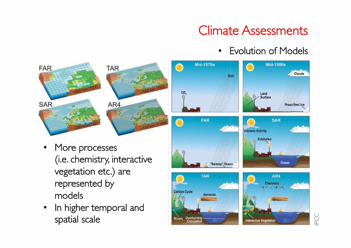
Climate Assessments

•  Evolution of Models

IPC

C

•  More processes ��(i.e. chemistry, interactive��vegetation etc.) are ��represented by��models

•  In higher temporal and��spatial scale

Climate Assessments

Type of Models •  Simple energy balance models very sophisticates ESMs

•  Atmosphere-Ocean General Circulation Models (AOGCMs)

•  Earth System Models (ESMs) ��AOGCM + Biogeochemical Cycles (Carbon, Sulphur, Ozone) •  Earth System Models in Intermediate Complexity (EMICs)��

Idealized or lower resolution. ��Applied to answer specific questions. ��

Needs less computational power

•  Regional Climate Models (RCMs)��Limited area models to downscale results of the lower

resolution models. It might also have multiple components! ht

tp://

ww

w.c

limat

echa

nge2

013.

org/

imag

es/r

epor

t/W

G1A

R5_

Cha

pter

09_F

INA

L.pd

f

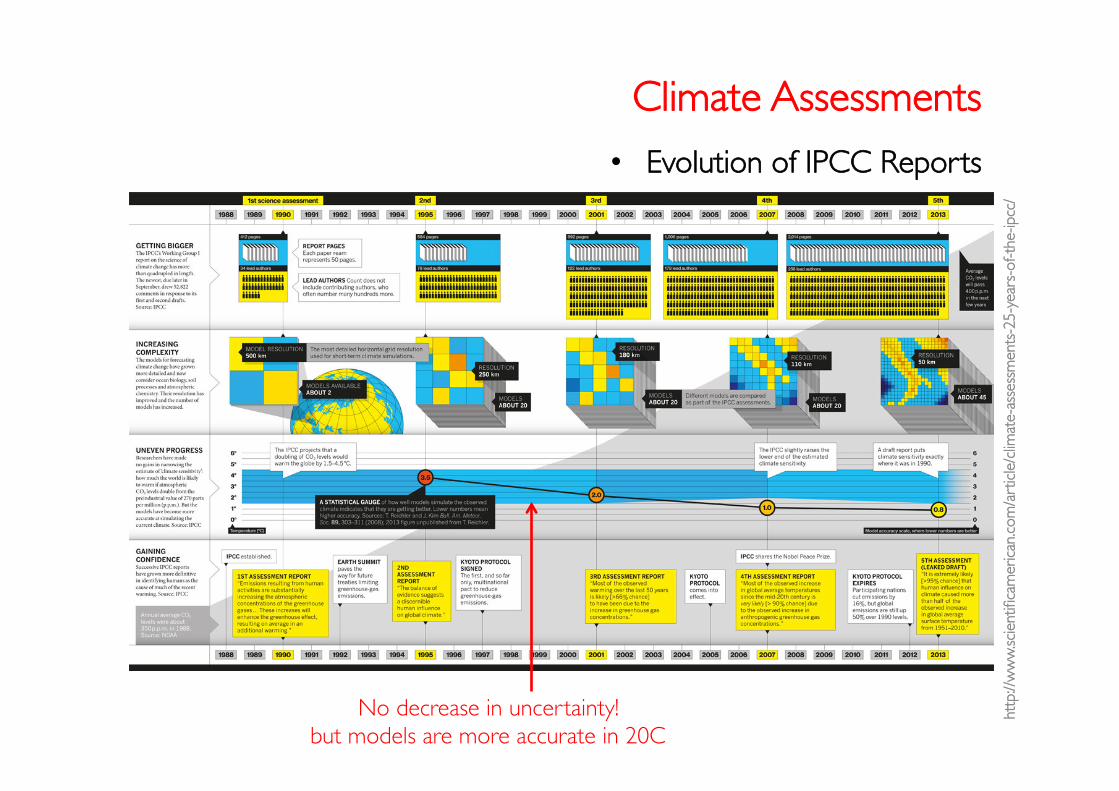
Climate Assessments

•  Evolution of IPCC Reports

http

://w

ww

.scie

ntifi

cam

eric

an.c

om/a

rtic

le/c

limat

e-as

sess

men

ts-2

5-ye

ars-

of-t

he-ip

cc/

No decrease in uncertainty! but models are more accurate in 20C

Evolution of Published Papers

•  Coupled Modeling Keyword: “Coupled climate model” (in Topic)

Keyword: “Earth System Model” (in Topic)

Sour

ce: W

eb o

f Sci

ence

What is Model Coupling?

•  It is a sophisticated way of simulate climate system and ��complex interactions between its components.

•  The individual components are not perfect !

•  Our theoretical understanding of climate is still incomplete, and certain simplifying assumptions are unavoidable when building ��

these models (Reichler and Kim, 2008) !

•  Coupled model does not always gives best results but help to understand interactions and processes between components !

Difficulties in Model Coupling?

•  Example from Atmosphere + Ocean Coupling

1.  Initial state of the ocean is not precisely known ��Lack of continuous and high resolution observations. ��

Remote sensing might help but covers only ocean surface and ��recent decades. The quality also depends on many issues

(atmospheric correction and used algorithm, coastal regions etc.)

2.  An imbalance in the surface flux (heat, momentum and freshwater) much smaller than the observational accuracy is enough to cause a

drifting of coupled GCM simulations into unrealistic states It is not easy tightly couple models that are written by different groups

High accuracy of conservation is needed!

http

://w

ww

.ipcc

.ch/

publ

icat

ions

_and

_dat

a/ar

4/w

g1/e

n/ch

1s1-

5-3.

htm

l

Model Coupling

•  But still, common trend is to create multi-component and ��multi-scale model applications and simulations

•  It needs close collaboration between different ��disciplines and research groups •  CESS: Computational Earth ��

System Science

Computer Science

Science & Engineering

Earth System Science

Meteorology

Oceanography

Land Surface + ��Hydrology

Chemistry

•  Designing efficient and scalable models •  Handling high volume of data (data compression, parallel I/O)

•  Automatization of model handling, reproducibility and metadata/provenance information collection

IS-ENES2, METAPHOR+CIM��Curator CMIPs (CMIP3/5) ESGF

Types of Model Coupling

There are two types of model coupling

1.  Offline Models run sequentially and the interaction between them is in

only one way. The simplest example is dynamical downscaling (GCM to RCM) or one-way nesting (RCM to RCM)

2.  Online In this case, models interact in both way and feedback mechanisms

among components represented (two way nesting, fully coupled atmosphere-ocean models or ESMs.)

Techniques for Model Coupling

The ESM components might be coupled using different programming approaches

more information in Valcke, 2009 EGU

1.  Merge individual model codes

single executable!

program ocn … ! read initial and boundary data call read() ! run model call run() ! write results to file … end program ocn

OCN easy to code, ��

portable

subroutine ocn (exchange vars) … ! read initial and boundary data call read() ! run model call run() ! write results to file … end subroutine ocn

program atm … ! read initial and boundary data call read() ! run model call run() ! write results to file … end program atm

host / parent

ATM

program atm … ! read initial and boundary data call read() ! run model call run() ! run ocn model call ocn(exchange vars) ! write results to file … end program atm

not flexible and��

generic

http

://w

ww

.cer

facs

.fr/~

coqu

art/

page

cerf

acs/

sem

inar

s/20

1405

_OA

SIS3

MC

T.pd

f




2.  Use existing communication protocols: MPI, InterComm …

program ocn … ! read initial and boundary data call read() ! run model call run() ! write results to file … end program ocn

OCN program atm … ! read initial and boundary data call read() ! run model call run() ! write results to file … end program atm

host / parent

ATM

program atm … ! receive exchange field call recv() ! run model call run() ! send exchange field call send() ! write results to file … end program atm

program ocn … ! receive exchange field call recv() ! run model call run() ! send exchange field call send() ! write results to file … end program ocn

mul9ple executable!

ATM OCN

existing code and concurrent

components not easy to

implement, not flexible and��

generic




3.  Use coupling framework & libraries: FMS, ESMF, MCT …

•  Code divided into units and calling interface redesigned ��(i.e. initialization, run and finalize)

•  Hierarchical model structures are supported

Existing codes must be restructured

flexible, efficient, portable, support to use generic utilities for interpolation, time

management and unit conversions), support both sequential and concurrent

components




4.  Use a coupler : OASIS, OASIS-MCT, MPCCI, PALM …

•  Coupler link the model components and handle coupling processes such as interpolation, synchronization etc.

•  Components models might be separate or single executable

flexible, efficient, portable, support to use generic utilities for interpolation, time

management and unit conversions), support concurrent components

multi-executable: ��more difficult to debug; harder to

manage for the OS and possible waste of resource if seq. execution enforced

What is driver / coupler ?

•  The driver can be defined as a “glue” •  It merges the different components of the modeling system

•  In general, the modeling system might be designed to have –  Single executable

–  Multiple executable (each component has an executable)

•  In the multiple executable case, the usage of the modeling system might be difficult

•  The driver is generally responsible for –  Interaction among the components: ��

exchange boundary data between ��the components, regridding etc.

–  Synchronization: ��to coordinate the time evolution ��of the physical models (coupling time step)

Coupled Model Design

•  Global Models (GCMs and ESMs) •  There is no single design and ultimate solution!

Kaitlin Alexander and Steve Easterbrook http

://cl

imat

esig

ht.fi

les.w

ordp

ress

.com

/201

1/08

/pos

ter.p

df

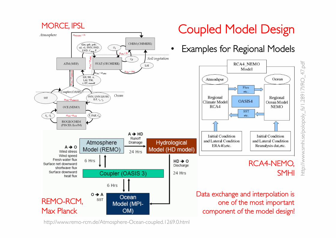
Coupled Model Design

•  Examples for Regional Models

http://www.remo-rcm.de/Atmosphere-Ocean-coupled.1269.0.html

MORCE, IPSL

REMO-RCM, ��Max Planck

RCA4-NEMO, ��SMHI ht

tp://

ww

w.sm

hi.se

/pol

opol

y_fs

/1.2

8917

!/RO

_47.

pdf

Data exchange and interpolation is ��one of the most important ��

component of the model design!

Common Problems in ES Modeling

•  The models are developed by different groups / organizations –  Various types of grids (curvilinear, regular, triangular etc.)

–  Written in various programming languages (Fortran, C, C++)

–  Different I/O strategies (ASCII, binary and netCDF) –  Different configuration mechanisms (simple ASCII files or well

structured XML files - CESM) –  Each component (ATM, OCN, etc.) has its own learning curve

–  Generally, does not follow common programming standards (CF conventions, GridSpec etc.)

•  Requirements: –  Need to know the way of “real programming” –  Need close collaboration between scientists and programmers

–  The standardization is very crucial. We need to think more generic solutions: standardized codes = better interoperability

Common Problems in Coupled Model Design

•  Need more attention –  Data exchange and interpolation between model grids

•  Support for different types of grids

•  Conservation of flux fields (high order conservative regridding?)

•  Extrapolation might be needed for unmatched land-sea masks. ��Exchange grid might help!

–  Self describing models •  Need to document a simulation or run

•  It is important for reproducibility

•  Both metadata and provenance��information needed for tracking

•  Is it possible to collect automatically?

–  Synchronization of multi-component��models •  Tools like OASIS and ESMF help!

adapted from Steve Easterbrook

Re-‐run and get same results

Re-‐run the code and get different results

Confirm results using a different method

Repeatability = ̸ Reproducibility

Interpolation / Regridding

•  The problem arises when numerical grid of the model components are not same (i.e. atmosphere and ocean) ?

•  There are two main types: –  Conservative –  Non-conservative

https://wiki.cc.gatech.edu/CW2013/images/8/89/201302_OASIS3MCT_CW2013.pdf


•  Conservative type regridding is used to preserve flux fields (i.e. moisture and heat fluxes)

•  It can be implemented to conserve field in –  Local: integral of the local patches are equal –  Global: integral of the source and destination grid is equal

•  The current tools uses 1st order ��conservative regridding –  The resource field might have artifacts ��

if the ration between source and ��destination grid resolution is high ��(i.e. atmosphere model in 50 km but ��ocean model 10 km)

http://www.earthsystemmodeling.org/presentations/pres_1002_siam_ryan.pdf

Qoi =

1Ao

Qanwni

n=1

N

! wni = !sin(lat)dlon

Cni!"


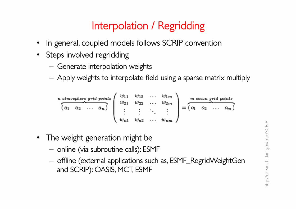
•  In general, coupled models follows SCRIP convention •  Steps involved regridding

–  Generate interpolation weights

–  Apply weights to interpolate field using a sparse matrix multiply

•  The weight generation might be

–  online (via subroutine calls): ESMF

–  offline (external applications such as, ESMF_RegridWeightGen ��and SCRIP): OASIS, MCT, ESMF

http

://oc

eans

11.la

nl.g

ov/t

rac/

SCR

IP

Peggy Li, 2010, ESMFvsSCRIP-v2.doc��http://pantar.cerfacs.fr/globc/publication/technicalreport/2012/SCRIP_ESMF_LiYan.pdf

•  SCRIP vs. ESMF_RegridWeightGen –  SCRIP does calculations in (lat,lon) space but ��

ESMF does it in (x,y,z) space –  Different area calculation for conservative remapping

–  SCRIP is serial but ESMF provide also parallel execution


ESMF Interpolation is currently used by ��NCL and ESMPy

•  Different model components with different land-sea mask –  Play with land-sea mask of each ��

components to match them •  It is hard and very time consuming

•  Must be repeated for each ��individual applications. It is not ��a generic solution

–  Use exchange grid (needs conservative type regridding)

–  Two step interpolation Interpolation + Extrapolation

Unmatched Land-sea Masks

OCN ATM Mismatch

orphan grid cell assigned to land (arbitrarily)

clipped

•  Two step interpolation ��(i.e. interpolation over ocean)

Unmatched Land-sea Masks

STEP 2 2.  Use result of previous step, ��

interpolate data from OCN to OCN ��from mapped grid points ��to unmapped ones using��nearest-neighbor type regridding

3.  Merge results of 1 and 2 to��create filled field

+

STEP 3 =

•  Still has problem in some applications (sharp gradient in some cases) but used in RegESM

•  Other extrapolation techniques?

Tha

nks

to E

SMF

Gro

up (

espe

cial

ly t

o Bo

b O

ehm

ke)

for

thei

r su

ppor

t an

d he

lp

STEP 1

1.  Interpolate from ATM to OCN��using bilinear interpolation. Use ��only sea grid points

mapped

unmapped

Automatization

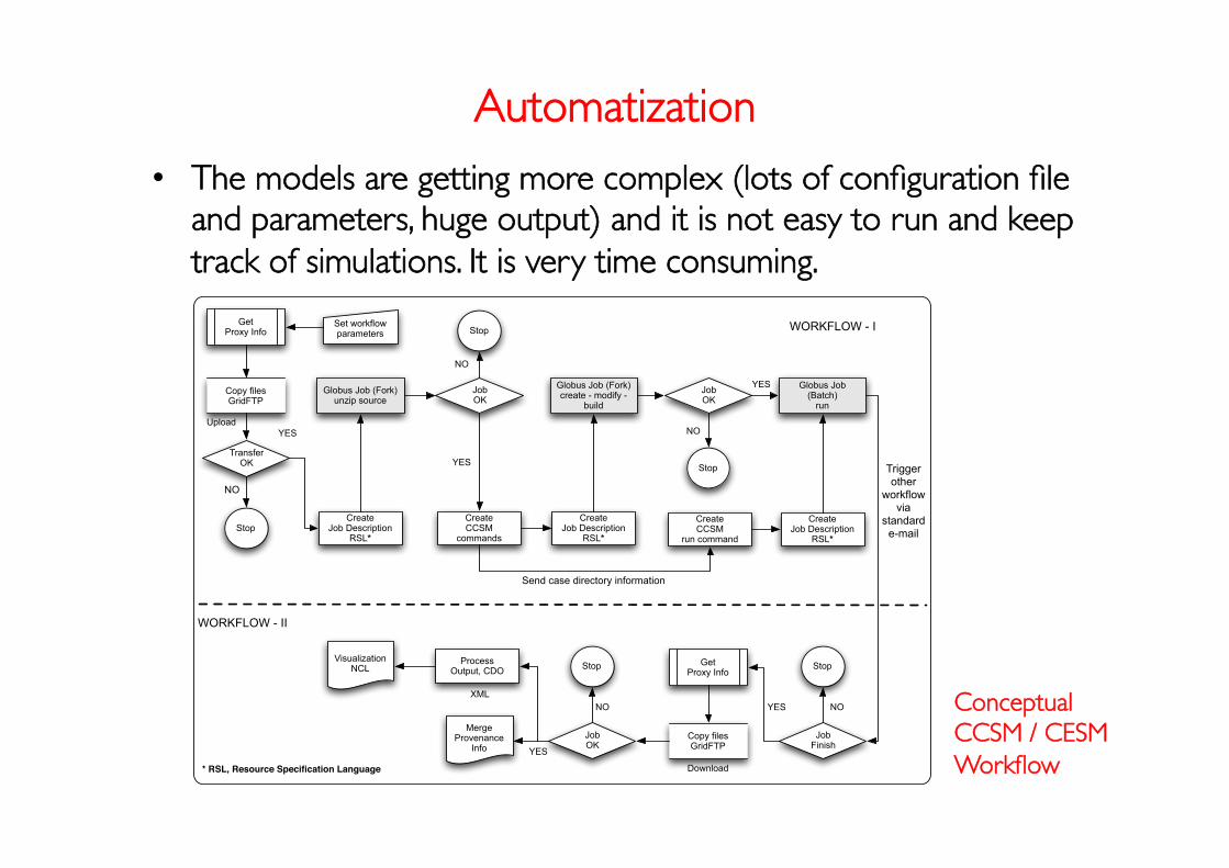
•  The models are getting more complex (lots of configuration file and parameters, huge output) and it is not easy to run and keep track of simulations. It is very time consuming.

Copy filesGridFTP

GetProxy Info

Globus Job (Fork)unzip source

TransferOK

StopCreate

Job DescriptionRSL*

JobOK

Stop

NO

YES

YES

Globus Job (Fork)create - modify -

build

NO

CreateJob Description

RSL*

CreateCCSM

commands

JobOK

Stop

NO

YES Globus Job (Batch)

run

CreateJob Description

RSL*

CreateCCSM

run command

Send case directory information

JobFinish

Stop

NO

Copy filesGridFTP

YES

Set workflowparameters

Download

Upload

MergeProvenance

InfoJobOK

Stop

NO

YES

XML

Trigger other

workflowvia

standarde-mail

ProcessOutput, CDO

VisualizationNCL

WORKFLOW - II

WORKFLOW - I

GetProxy Info

* RSL, Resource Specification Language

Conceptual CCSM / CESM Workflow

Automatization

•  Scientific workflow tools might help to simplify the regular tasks! •  Teragrid:

creates WS-GRAM XML job description files automatically

build model collect

provenance and metadata info

run model Turu

ncog

lu, C

G: 2

011,

EM

S: 20

13 a

nd E

SM B

ook

(Vol

. 5):

2012

Automatization

•  Scientific workflow tools might help to simplify the regular tasks! •  Modified workflow for conventional cluster

workflow wide global��parameters

build model

collect provenance and��metadata info

run model

Turu

ncog

lu, C

G: 2

011,

EM

S: 20

13 a

nd E

SM B

ook

(Vol

. 5):

2012

Modeling Experiences in ICTP

•  RegCM –  Regional Climate Model (hydrostatic)

–  Sophisticated sub-grid parameterization

–  Coupled with Atm. Chemistry, 1D Lake and Slab Ocean Models •  AGCM (Speedy) – Intermediate Complexity Model

–  Simplified GCM (Molteni and Kucharski)

–  Spectral Model (hydrostatic) –  Slab models for land and sea-ice

•  ICTP-NEMO Coupled Model –  Speedy + NEMO + OASIS3

–  T30/L8 and 2 deg (+ equatorial refinement 1/3 deg)

–  Supports one and two way coupling

http

://in

dico

.ictp

.it/e

vent

/a10

154/

sess

ion/

6/co

ntrib

utio

n/4/

mat

eria

l/0/0

.pdf

New regional modeling system (RegESM)?

•  To design easy to use and extend modeling system –  ENEA’s PROTHEUS system uses MITgcm+RegCM3+OASIS

–  It is not easy to use, extend and upgrade (It uses multiple executable, no online interpolation support, hard to add new component such as wave)

•  To support Med-CORDEX –  Set of coordinated experiments to better understand

Mediterranean climate: standalone and coupled RCMs –  It would be good to have another regional coupled modeling

system that uses different model components

•  To gain experience about design and use of coupled modeling systems –  The applications of coupled modeling system getting increased in

last decade along with the rapid development in HPC

Evolution of RegESM •  The first prototype version is created in 2012

–  There were no driver

–  RegCM was host the whole coupled modeling system

–  Single ocean component was supported (ROMS) –  Poor energy conservation (for exchange fields)

–  Applied to Caspian Sea (Turuncoglu et al., 2013, GMD)

•  Then, more generic version is designed and released in 2013 –  Centralized driver using ESMF’s NUOPC layer (via connectors)

–  All the components plugged into driver (less dependence to the model component code)

–  Support for multiple ocean model (ROMS and MITgcm)

–  Energy conservation is improved (global conservation) –  Support to extrapolation (land-sea mask mismatch)

–  Applications: Mediterranean, Black Sea and Caspian Sea

RegESM Design & Components

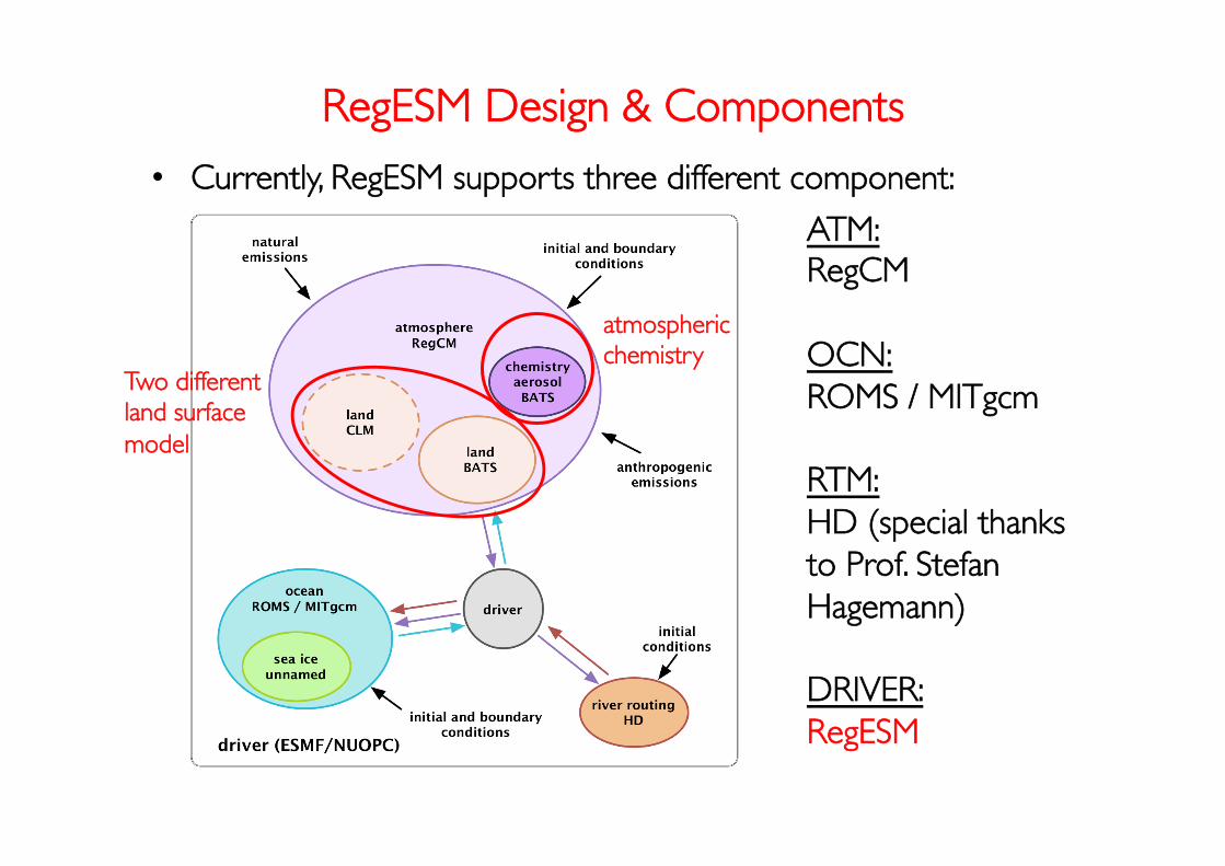
•  Currently, RegESM supports three different component: �� ATM:

RegCM OCN: ROMS / MITgcm RTM: HD (special thanks to Prof. Stefan Hagemann) DRIVER: RegESM

atmospheric��chemistry

Two different land surface ��model

Driver Design in ESMF/NUOPC

•  The current driver uses only “connector” component (NUOPC)

•  The driver defines; –  The model components (i.e. RegCM, ROMS) – grid, fields, states etc.

–  Coupler component (connector) –  Global clock and calendar

•  and synchronizes the sequence of actions http

s://w

ww

.ear

thsy

stem

cog.

org/

proj

ects

/nuo

pc/

Driver Designs in ESMF/NUOPC •  Different designs are possible with NUOPC layer •  The mediator approach is much more efficient when the

number of components increase

Simple Coupling ��with Connectors

ATM+OCN

Coupling through a Mediator

Connectors

http

s://w

ww

.ear

thsy

stem

cog.

org/

proj

ects

/nuo

pc/

Run Sequences in ESMF/NUOPC

•  The NUOPC Layer is capable of implementing many different coupling schemes –  Explicit: ��

Exchange data in same time. Two ��connector (i.e. backward and ��forward)

–  Explicit with slow and fast ��clock support:��Different interaction time ��step among the components

–  Semi-implicit (leap-frog style ��interaction)

–  Fully-implicit

ATM

OCNt=0h t=1h ...

ATM-OCNOCN-ATM

coupling time

Ex: 1 hour

EXPLICIT RUN SEQUENCE

Initializationof models

ATM

OCNt=0h t=1h ...

SEMI-IMPLICIT RUN SEQUENCE

ATM

OCNt=0h t=1h ...

IMPLICIT RUN SEQUENCEt=1/2 h

2

34 5

1 2

1

2

34

2

1

2

34

2

34 5

4

3

1

3

4

data exchangemodel integrate

x2

16

16

7 7

Run Sequence in RegESM

•  The RegESM might use both explicit and semi-implicit coupling schemes along with the support of fast and slow time steps. –  Fast interaction between ATM and OCN

–  Slow interaction between ATM and RTM, RTM-OCN –  Here, RTM is optional component

Example for 3 component and explicit coupling:

Sequential vs. Concurrent Execution

•  The modeling system supports two different approach to run the model components.

•  In sequential mode: model components are run in order

•  In concurrent mode: all models are active at same time (it does not allow overlapping of the used PETs – cores / CPUs)

Repository and Project Home

•  The RegESM project is hosted by GitHub –  https://github.com/uturuncoglu/RegESM

•  The project home page

Implemented by using CoG1

http://cess.be.itu.edu.tr/projects/regesm/

I) https://www.earthsystemcog.org/projects/cog/

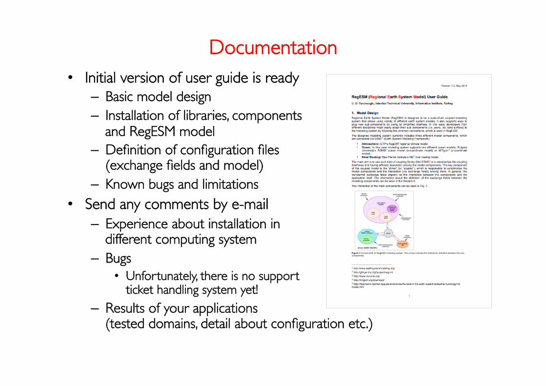
Documentation •  Initial version of user guide is ready

–  Basic model design –  Installation of libraries, components ��

and RegESM model –  Definition of configuration files��

(exchange fields and model) –  Known bugs and limitations

•  Send any comments by e-mail –  Experience about installation in ��

different computing system –  Bugs

•  Unfortunately, there is no support ��ticket handling system yet!

–  Results of your applications ��(tested domains, detail about configuration etc.)

Questions!

Contact:

[email protected]

overview of model coupling in earth system sciences and

Documents