output gaps and robust monetary policy rules · output gaps and robust monetary policy rules...

Output Gaps and Robust Monetary Policy Rules∗

Roberto M. Billi

Sveriges Riksbank Working Paper Series No. 260

Revised December 2018

Abstract

Policymakers often use the output gap to guide monetary policy, even though inflation

and nominal gross domestic product (GDP) are measured more accurately in real time.

Employing a small New Keynesian model with a zero lower bound (ZLB) on nominal

interest rates, this article compares the performance of monetary policy rules that are

robust to persistent measurement errors. It shows that, in the absence of the ZLB,

the central bank should focus on stabilizing inflation rather than nominal GDP. But

present the ZLB, a policy that seeks to stabilize nominal GDP improves substantially

the tradeoffs faced by the central bank.

Keywords: measurement errors, nominal targets, optimal monetary policy

JEL: E31, E52, E58

∗I thank for valuable comments Yunus Aksoy, Pierpaolo Benigno (coeditor), Fabio Canova, Larry Chris-tiano, Emmanuel De Veirman, Andy Filardo, Jordi Galí, Tor Jacobson, Per Jansson, Keith Kuester, StefanoNeri, Damjan Pfajfar, Charles Plosser, Ricardo Reis, Frank Smets, Ulf Söderström, Lars Svensson, JohnTaylor, Robert Tetlow, David Vestin, Karl Walentin, John Williams, Mike Woodford, Andreas Wörgötter,seminar participants at Banca d’Italia, Bank of England, Copenhagen Business School, Federal Reserve Bankof Philadelphia, Joint Seminar Series of the ECB-CFS-Bundesbank, Sveriges Riksbank, Tilburg University,Uppsala University, as well as conference participants at AEA, Joint French Macro Workshop at Banque deFrance, Macro Workshop at De Nederlandsche Bank, Midwest Macroeconomics Meeting, Monetary PolicyChallenges from a Small Country Perspective at National Bank of Slovakia, and SCE. I gratefully acknowledgethe ECB’s hospitality while working on this project in 2018. The views expressed herein are solely the re-sponsibility of the author and should not be interpreted as reflecting the views of Sveriges Riksbank. Addresscorrespondence to: Roberto M. Billi, Monetary Policy Department, Sveriges Riksbank, SE-103 37 Stockholm,Sweden; e-mail: [email protected].

1

1 Introduction

In monetary policy analysis, a commonly used measure of economic activity is the output

gap, which is a gauge of how far the economy is from its productive potential. The output

gap is conceptually appealing as an indicator to help guide policy because it is an important

determinant of inflation developments. A positive output gap implies an overheating economy

and upward pressure on inflation. By contrast, a negative output gap implies a slack economy

and downward pressure on inflation. Thus, if available, accurate and timely estimates of the

output gap can play a central role in the conduct of effective monetary policy. A positive

output gap prompts the central bank to cool an overheating economy by raising policy rates,

whereas a negative output gap prompts for adding monetary stimulus.

In practice, however, the output gap is a noisy signal of economic activity. Estimates of

the output gap are often subject to large revisions, even long after the time policy is actually

made.1 Thus, there is broad interest in finding monetary policies that are robust to persistent

errors in measuring the output gap. As Taylor and Williams (2010) explained, one view is

that in simple policy rules the optimal coeffi cient on the output gap declines in the presence

of noise in measuring the gap. The logic for this result is straightforward. The reaction to the

mismeasured output gap adds unwanted noise to the setting of monetary policy, which causes

unnecessary fluctuations in output and inflation. Such adverse effects of noise can be reduced

by lowering the coeffi cient on the output gap in the policy rule.

At the same time, many argue for greater policy activism when the zero lower bound

(ZLB) on nominal interest rates constrains policy.2 The inability to reduce the policy interest

rate below its effective lower bound can limit, or even impair, the ability of monetary policy

to stabilize output and inflation. As Reifschneider and Williams (2000) showed, increasing

the coeffi cient on the output gap in simple policy rules can improve economic performance.

1Measuring the output gap involves two complications. First, potential output cannot be measured directly,so must be estimated. Second, GDP data are regularly revised as statistical agencies incorporate more completesource information and new methodologies into the published data. As Orphanides and van Norden (2002)showed, estimating potential output is the main source of errors in measuring the output gap.

2This article adopts the standard practice of referring to a zero lower bound on nominal interest rates.The recent experience with negative nominal interest rates in Denmark, Japan, Sweden, Switzerland, and theeurozone suggests the effective lower bound is somewhat below zero. See Svensson (2010) for a discussion.

2

An active response to the output gap prescribes greater monetary stimulus before and after

episodes when the ZLB constrains policy, which lessens deflationary pressures when the ZLB

constrains policy. But there are clear limits to such an approach, as it generally increases

the volatility of inflation and interest rates. A large coeffi cient on the output gap can be

counterproductive, especially when the output gap is mismeasured.

In light of such concerns, another perspective is that central banks should ignore the

output gap altogether to focus strictly on stabilizing inflation or seek instead to stabilize the

level of nominal gross domestic product (GDP). Nominal GDP level targeting is particularly

appealing for two reasons. First, monetary policy is then expected to be more robust to errors

in the measurement of economic activity, because revisions to GDP are typically smaller than

revisions to the output gap. Estimates of GDP are not prone to errors from estimating

potential output. Second, the central bank is also required to make up for any past shortfalls

from its nominal GDP target, which ensures greater policy stimulus during ZLB episodes.

This article, thus, studies the performance of such monetary policy rules in a small New

Keynesian model, with the central bank facing persistent errors in the measurement of eco-

nomic conditions and a ZLB constraint.3 In the model, several types of structural and noise

shocks buffet the economy. On the supply side, technology shocks push output gaps and infla-

tion in the same direction, whereas cost-push shocks instead cause an inflation-output tradeoff.

On the demand side, adverse demand shocks and the ZLB constraint create a tradeoffbetween

stabilizing current and future output, because it is desirable for the central bank in a ZLB

episode to promise to induce an expansion after the ZLB episode.4 Moreover, the central

bank faces persistent noise shocks in the setting of monetary policy, which creates a tradeoff

between fluctuations in the economy from structural shocks and those from noise shocks.

The stylized model offers a clear illustration of such tradeoffs in the evaluation of the

monetary policy rules. Before proceeding to the evaluation, the model is calibrated to recent

3This analysis assumes the private sector possesses full information about the state of the economy inreal time, which implies the model can be treated as structurally invariant under different policies. See Aoki(2003, 2006) and Svensson and Woodford (2004) for a discussion.

4The promise is credible if the central bank commits to making up for past shortfalls from its target, as isthe case with an inertial Taylor rule or with a nominal GDP level target.

3

U.S. data, with the conduct of monetary policy described by a simple rule often used in policy

analysis, namely a version of the Taylor rule with interest-rate smoothing. In the calibration

of the model, the structural shocks are persistent to generate propagation in the model as

in the data. The noise shocks are persistent to reflect historical revisions of the data. Also

considered is the optimal commitment policy, to be used as a benchmark for the evaluation.

The monetary policy rules are then ranked in terms of performance, based on the model’s

social welfare function.

With the calibrated model, I study the extent to which persistent errors in the measurement

of economic conditions and a ZLB constraint adversely affect the performance of the two

targeting rules and inertial Taylor rule, relative to the optimal commitment policy. The

analysis produces three main results. First, under the optimal commitment policy, although

measurement error and the ZLB constraint are both a source of fluctuations in output and

inflation, social welfare is more severely affected by the ZLB constraint. As a second main

result, the ZLB constraint plays a critical role for the ranking of two targeting rules. In the

absence of the ZLB, the central bank should focus on stabilizing inflation rather than nominal

GDP. But present the ZLB, a policy that seeks to stabilize the level of nominal GDP improves

substantially the tradeoffs faced by the central bank. And third, if monetary policy becomes

more severely constrained by the ZLB, social welfare is more severely affected under a targeting

rule that does not require to make up for past shortfalls from the target.

In the previous literature, in the aftermath of the financial crisis and Great Recession,

proposals for nominal GDP level targeting include Hatzius and Stehn (2011, 2013), Sumner

(2011, 2014), Woodford (2012, 2013), Frankel (2013), and Billi (2017), among others.5 But

none of these articles takes into account that central banks face persistent errors in the mea-

surement of economic conditions. In another strand of literature, studies about the design

of monetary policies that are robust to measurement error include Orphanides et al. (2000),

Orphanides (2001, 2003), Rudebusch (2002), Smets (2002), Ehrmann and Smets (2003), Aoki

5There is also an extensive literature on the notion of nominal income growth targeting, at first suggestedby Meade (1978) and Tobin (1980) and then studied by Bean (1983), Taylor (1985), West (1986), McCallum(1988), Clark (1994), Hall and Mankiw (1994), Jensen (2002), Walsh (2003), and Billi (2011b), among others.

4

(2003, 2006), Svensson and Woodford (2003, 2004), Boehm and House (2014), and Garín,

Lester and Sims (2016), and others. But these articles do not take into account a ZLB

constraint. Gust, Johannsen and Lopez-Salido (2017) study the interaction between mismea-

surement of the state of the economy and a ZLB constraint but for tractability need to assume

the mismeasurement is not persistent. Relative to the previous literature, the contribution of

this article is to show that the ranking of the monetary policy rules depends crucially on the

likelihood of hitting the ZLB constraint.

The article proceeds as follows. Sections 2 describes the model and monetary policy rules.

Section 3 presents the model outcomes and policy evaluation. Section 4 concludes. The

Appendix contains technical details of the model solution and additional results.

2 The model

I use a small New Keynesian model as described in Woodford (2010). I describe the conduct

of monetary policy with targeting rules, and with a simple rule to be used for the calibration

of the model. In each of the policy frameworks considered, the central bank faces persistent

errors in the measurement of economic conditions and a ZLB constraint. I explain the features

of this model and the equilibrium, and then calibrate the model to U.S. data.

2.1 Private sector

The behavior of the private sector is described by two structural equations, log-linearized

around zero inflation, which represent the demand and supply sides of the economy. The

economy is buffeted by persistent demand and supply shocks.

On the demand side of the economy, the Euler equation describes the representative house-

hold’s expenditure decisions,

yt = Etyt+1 − ϕ (it − r − Etπt+1 − vt) , (1)

where Et denotes the expectations operator conditional on information available at time t. yt

5

is output measured as the log-deviation from a trend. πt is the inflation rate, the log-change

of prices from the previous period,

πt ≡ pt − pt−1. (2)

And it ≥ 0 is the short-term nominal interest rate, which is the instrument of monetary

policy and is constrained by a ZLB. r > 0 is the steady-state interest rate.6 ϕ > 0 is the

interest elasticity of real aggregate demand, capturing intertemporal substitution in household

spending. The demand shock, vt, represents other spending, such as government spending,

which has asymmetric effects on the economy due to the ZLB constraint. A positive demand

shock can be countered entirely by raising the nominal interest rate, whereas a large adverse

shock that leads to hitting the ZLB causes an economic downturn.

On the supply side of the economy, the Phillips curve describes the optimal price-setting

behavior of firms, under staggered price changes à la Calvo,

πt = βEtπt+1 + κxt + ut, (3)

where β ∈ (0, 1) is the discount factor of the representative household, determined as 1/ (1 + r).

The slope parameter κ > 0 is a function of the structure of the economy.7 xt ≡ yt − ynt is the

output gap in the economy. ynt is the natural rate of output, or potential output, the output

deviation from the trend that would prevail in the absence of any price rigidities, which rep-

resents a technology shock. A positive technology shock implies slack in economic activity and

downward pressure on prices, whereas a negative shock implies a strong economy and puts

upward pressure on prices. Moreover, ut is a cost-push shock, or mark-up shock resulting from

variation over time in the degree of monopolistic competition between firms, which creates an

inflation-output tradeoff for monetary policy.

6Thus, it − r − Etπt+1 is the real interest rate in deviation from steady state.7In this model κ = (1− α) (1− αβ)α−1

(ϕ−1 + ω

)(1 + ωθ)

−1, where ω > 0 denotes the elasticity of a firm’sreal marginal cost. θ > 1 is the price elasticity of demand substitution with firms in monopolistic competition,and thus the seller’s desired markup is θ/ (θ − 1). Moreover, α ∈ (0, 1) is the share of firms keeping pricesfixed each period, so the implied duration between price changes is 1/ (1− α).

6

In this model economy, the three types of exogenous structural shocks (ynt , ut, vt) are

assumed to follow AR(1) stochastic processes, with first-order autocorrelation parameters

ρj ∈ [0, 1) for j = yn, u, v. Moreover, σεjεjt are the innovations that buffet the economy,

which are independent across time and cross-sectionally, and normally distributed with mean

zero and standard deviations σεj > 0.

Finally, the monetary policy rules to be considered are evaluated based on the model’s

social welfare function, a second-order approximation around zero inflation of the lifetime

utility function of the representative household,

E0

∞∑t=0

βt[π2t + λ (xt − x∗)2

], (4)

where λ = κ/θ is the weight assigned to stabilizing the output gap relative to inflation. x∗ is

the target level of the output gap, which stems from monopolistic competition and distortion

in the steady state. Output subsidies are assumed to offset the monopolistic distortion so that

the steady state is effi cient, x∗ = 0. As a result, in this analysis, there is no inflation bias but

there is a stabilization bias due to suboptimal monetary policy and mark-up shocks, even if

monetary policy is not constrained by the ZLB.

2.2 Monetary policy

I consider four monetary policy frameworks, namely a simple policy rule, two targeting rules,

and optimal commitment policy. In each of these policy frameworks, the central bank faces a

ZLB constraint and persistent errors in the measurement of economic conditions. Regardless

of the ZLB constraint, the measurement errors lead to policy mistakes and therefore cause a

deterioration in economic performance.

The first policy framework is an inertial Taylor rule subject to a ZLB constraint, along

the lines of Taylor and Williams (2010),

it = max[0, φii

ut−1 + (1− φi) (r + φππ

ot + φxx

ot )], (5)

7

where φπ and φx are positive response coeffi cients on observed inflation, πot = πt + eπt , and

the observed output gap, xot = xt + ext , respectively. eπt and ext represent noise shocks or

measurement errors.8 This rule incorporates smoothing in the behavior of the interest rate,

through a positive value of the coeffi cient φi ∈ [0, 1). Moreover, iut−1 denotes an unconstrained

or notional interest rate, the preferred setting of the policy rate in the previous period that

would occur absent the ZLB constraint. Thus, the policy rate is kept below the notional

interest rate following an episode when the ZLB is a binding constraint on policy.9 This

inertial Taylor rule is used for the calibration of the model (Section 2.4).

The next two policy frameworks considered are targeting rules subject to a ZLB constraint.

In other words, rather than following a simple policy rule, the central bank aims to stabilize

a target variable by re-optimizing to the extent possible its policy decision (it ≥ 0) in each

period. One of the targeting rules considered is strict inflation targeting,

πot = 0 subject to it ≥ 0, (6)

where the central bank seeks to stabilize inflation without any concern for output stability

and, therefore, transfers the burden of shocks onto output. This targeting rule does not involve

any inertia in the setting of monetary policy, because the current policy decision disregards

past economic conditions and past misses from the target.

The other targeting rule considered in this analysis is nominal-GDP-level targeting,

not = 0 subject to it ≥ 0, (7)

where not is observed nominal GDP, not = nt + ent . Specifically, nt = pt + yt is actual nominal

GDP measured as the log-deviation from a trend, and ent is a noise shock. With this targeting

rule, the central bank seeks to stabilize nominal GDP, as opposed to focusing entirely on

8In the data, both inflation and output gaps are subject to persistent revisions (Section 2.4). Thus, inthe model, instead of using only one noise shock to reduce the number of state variables, both eπt and e

xt are

present for the policy rule to be consistent with the real-time data.9Such an approach implies that the central bank compensates to some extent for the lost monetary stimulus

due to the presence of the ZLB, even though the central bank does not commit to making up for past shortfallsfrom a nominal-level target.

8

inflation stability, which now requires the burden of shocks to be shared by inflation and

output. This targeting rule involves inertia in the behavior of monetary policy because the

current policy decision depends on the past price level, as pt ≡ pt−1 + πt.

Next, as a benchmark for the evaluation of these monetary policy rules, I use the optimal

commitment policy. In such a policy framework, the central bank is assumed able and willing

to fully commit to its policy announcements, to maximize the welfare of the representative

household. In this ideal policy framework, the central bank’s objective function is given by

minit≥0

E0

∞∑t=0

βt[(πot )

2 + λ (xot )2] ,

where the central bank seeks to stabilize to the extent possible inflation and the output gap,

subject to a ZLB constraint. This objective function generally differs from the social welfare

function, equation (4), because the central bank faces persistent errors in the measurement

of inflation and the output gap. These measurement errors cause a deterioration in economic

performance, regardless of the ZLB constraint.

In these four monetary policy frameworks, the exogenous noise shocks (eπt , ext , e

nt ) are

assumed to follow AR(1) stochastic processes, with first-order autocorrelation parameters

ρj ∈ [0, 1) for j = eπ, ex, en. Moreover, σεjεjt are the shock innovations buffeting the economy,

which are independent across time and cross-sectionally, and normally distributed with mean

zero and standard deviations σεj > 0.

2.3 Equilibrium

At equilibrium, the policymaker chooses a policy based on a response function y (st) and a state

vector st. The st includes the endogenous variables, the structural shocks, as well as the noise

shocks affecting the central bank’s observation of economic conditions. The corresponding

expectations function is then

Ety (st+1) =

∫y (st+1) f (εt+1) d (εt+1) ,

9

where f (·) is a probability density function of future innovations, both in the structural and

noise shocks, which buffet the economy. In such a setting, an equilibrium is given by a re-

sponse function and expectations function, y (st) and Ety (st+1), which satisfy the equilibrium

conditions, derived in Appendix A.1.

Ignoring the existence of uncertainty about the future state of the economy, the model can

be solved with standard numerical methods, as done in Orphanides and Wieland (2000), Reif-

schneider and Williams (2000), Williams (2009), Levin et al. (2010), Coibion, Gorodnichenko,

andWieland (2012), and Guerrieri and Iacoviello (2015), among others. When the ZLB threat-

ens, however, the mere possibility of hitting the ZLB causes expectations of a future economic

downturn and therefore prompts for adding policy stimulus today, as shown by Adam and

Billi (2006, 2007), and Nakov (2008), and others. In this analysis, as in Billi (2011a, 2017),

I use a numerical procedure that accounts for the ZLB constraint and uncertainty about the

evolution of the economy.10

2.4 Baseline calibration

The model economy is calibrated to revised U.S. data for recent decades, as in Billi (2017),

with monetary policy described by the inertial Taylor rule (5) that features prominently in

Federal Reserve discussions. The values of the rule coeffi cients are taken from English, Lopez-

Salido and Tetlow (2015), with φπ set to 1.5, φx set to 1/4 (quarterly rates) and φi set to 0.85.

The rule thus accounts for smoothing in the setting of the policy interest rate.

The values of the structural parameters are also standard in the related literature. Specif-

ically, β is set to 0.993, to imply r equal to 3% annual. ϕ is set to 6.25.11 The implied

parameters κ and λ are then equal to 0.024 and 0.003 (quarterly), respectively. Regarding the

structural shocks, ρyn,u,v are set to 0.8, to generate persistent effects on the economy. σyn,v are

set to 0.8% (quarterly) to try to replicate respectively the volatility of output and nominal in-

terest rates in the data, whereas σu is set to 0.05% (quarterly) to match the inflation volatility

10See Appendix A.2 for a description of the algorithm used to solve the model.11α is set to 0.66, so the duration between price changes 1/ (1− α) is 3 quarters. θ is set to 7.66, so the

markup over marginal cost θ/ (θ − 1) is 15%. Moreover, ω is set to 0.47.

10

in the data.12 Overall, as Billi (2017) showed, with the inertial Taylor rule and revised data,

the model does a fairly good job in replicating the relevant features of recent U.S. data.13

The calibration of the noise shocks is obtained fitting historical revisions of U.S. data,

as done in Billi (2011b). Real-time estimates reflect information actually available to poli-

cymakers in each quarter, whereas revised estimates reflect information as available at the

end of the sample period. The difference between revised and real-time estimates is the his-

torical revision of the data. (σεeπ , σεex , σεen) are set to match the volatility of data revisions

(0.3, 1.7, 1.1) in percent annual. (ρeπ , ρex , ρen) are set to match the persistence of data revi-

sions (0.7, 0.85, 0.8).14 Thus, reflecting historical revisions of the data in the calibrated model,

the measurement errors are notably larger and more persistent for the output gap than for

nominal GDP and inflation.

3 The policy evaluation

With the calibrated model, I study the extent to which persistent measurement errors and a

ZLB constraint adversely affect the performance of the two targeting rules and inertial Taylor

rule, relative to the optimal commitment policy. Exploring a range of calibrations for the

supply and demand shocks buffeting the economy, I show that the ranking of these monetary

policy rules depends crucially on the likelihood of hitting the ZLB constraint.

12The inflation rate is measured as the continuously compounded rate of change in the seasonally adjustedpersonal consumption expenditures chain-type price index less food and energy (source BEA). Output ismeasured as the log deviation from trend in seasonally adjusted gross domestic product (source BEA). Theoutput gap is calculated as the deviation of real gross domestic product from potential, as a fraction of potentialusing seasonally-adjusted data (source CBO). And the nominal interest rate is measured as the average effectivefederal funds rate (source Fed Board). The sample period used to calibrate the structural shocks is the sameas in Billi (2017), 1984Q1-2014Q4, which ensures the results are directly comparable. Moreover, extending thesample to the latest available data does not affect the good fit of the model to the data. Real-time and reviseddata are obtained from archival economic data available at the St. Louis Fed, https://alfred.stlouisfed.org.13Still, output and inflation are somewhat less persistent in the model results than in the data because this

basic model, for the sake of simplicity, does not allow for structural propagation mechanisms that give rise tooutput and inflation inertia. As a consequence, the stylized model understates the frequency and duration ofZLB episodes. With the inertial Taylor rule and revised data, the model predicts that the policy rate hits theZLB about 4 percent of the time, and the expected duration of a ZLB episode is about 4 quarters (Table 2).In actuality, the federal funds rate has been near the ZLB from the end of 2008 to the end of 2015. See Section2.4 of Billi (2017) for further details of the model calibration and fit to the data.14The half-lives of the noise shocks log (0.5) /log (ρeπ , ρex , ρen) are equal to (1.9, 4.3, 3.1) quarters.

11

3.1 Response to shocks

As the first step in the evaluation of the monetary policy rules, Figures 1 and 2 show the

evolution of the economy when hit by the different types of structural and noise shocks in the

model.15 The first figure displays responses under the optimal commitment policy and inertial

Taylor rule, whereas the second figure displays responses under the two targeting rules. In

both figures, shown are the responses of inflation, the output gap, and the nominal interest

rate.

[Figures 1 and 2 about here]

Regarding the supply shocks, the top panel of the two figures shows the response to a

positive technology shock, which implies slack in economic activity and downward pressure on

prices. The outcome, however, depends on the monetary policy rule considered. With nominal

GDP level targeting (figure 2, solid black line) both the output gap and inflation fall, whereas

under the other three policy frameworks the economy is generally stabilized. In other words,

in contrast to the other policy frameworks, nominal GDP level targeting fails to insulate the

economy from technology shocks, conditional on no other shocks buffeting the economy.

The second panel shows the response to a positive mark-up shock, which implies upward

pressure on prices and creates an inflation-output tradeoff for monetary policy. Facing such

a tradeoff, under strict inflation targeting (figure 2, dashed red line) inflation is completely

stabilized and output falls notably, whereas under the other three policy frameworks inflation

rises and output falls. The reason is that, in contrast to the other policy frameworks, strict

inflation targeting transfers the burden of mark-up shocks onto output. The other policy

frameworks require instead the burden of shocks to be shared by inflation and output.

Regarding the remaining shocks in the model, the third panel of the figures shows the

response to a negative demand shock, which exerts downward pressure on output and prices.

15Shown are expected paths after three-standard-deviation shocks, using the baseline calibration describedin Section 2.4. The expected paths are obtained by averaging across 10,000 stochastic simulations. Regardingthe paths shown in Figure 1, both inflation and the output gap are assumed to be mismeasured at the sametime. If instead only inflation or the output gap is mismeasured, the resulting paths would be of similar shapebut smaller size than the ones displayed in the figure.

12

Given the size of the shock, under each policy framework, the weakness of the economy prompts

the central bank to cut the nominal interest rate all the way to the ZLB. During the ZLB

episode, both output and inflation fall to a greater extent under strict inflation targeting,

compared to the other policy frameworks considered. The reason is that, as noted earlier,

strict inflation targeting does not involve any inertia in the setting of monetary policy.

Finally, the bottom panel of the figures shows the response to a positive noise shock

or measurement error, which implies the central bank incorrectly assumes there is upward

pressure on prices. As a consequence of such a measurement error, under each policy framework

considered, the central bank mistakenly tightens the stance of monetary policy and therefore

causes inflation and output to fall.16

3.2 Economic performance

The ability of the central bank to stabilize the economy is adversely affected by persistent

measurement errors and a ZLB constraint. To illustrate, Table 1 summarizes the performance

of the optimal commitment policy, in four different cases.

[Table 1 about here]

In the first case there is neither measurement error nor ZLB in the model, in the second

there is measurement error only, in the third instead there is the ZLB only, and in the fourth

there are both measurement error and ZLB. The table reports for each case the expected fre-

quency and duration of ZLB episodes, as well as the welfare loss due to business cycles.17 As

the table shows, taking into account either measurement error or the ZLB causes a deteriora-

tion in economic performance, as both inflation and output become more variable. However,

economic performance is more severely affected by the ZLB.18

I now rank the monetary policy rules in terms of performance, relative to the optimal

commitment policy, and also study whether the ranking depends on the measurement error16As the real interest rate (not shown) is higher, the stance of monetary policy is tightened.17To calculate the welfare loss, first the value of the objective function (4) is obtained by averaging across

10,000 stochastic simulations each 1,000 periods long after a burn-in period. This value is then converted intoa permanent consumption loss, as explained in Appendix A.3.18The total welfare loss is 0.06 with measurement error only but rises to 0.08 with the ZLB only (Table 1).

13

and ZLB constraint. Table 2 summarizes the performance of each policy framework, again in

the four cases. Each case is in a separate panel. In the first case, that is in the absence of

measurement error and ZLB in the model, strict inflation targeting results in a smaller total

welfare loss than nominal GDP level targeting. With strict inflation targeting the burden of

shocks is transferred onto output, but under nominal GDP level targeting the shocks affect

to a greater extent the volatility of inflation. Moreover, both these targeting rules perform

better than the inertial Taylor rule. This ranking of the monetary policy rules is obtained also

in the second case, that is in the presence of only measurement error in the model. However,

because of the measurement error, strict inflation targeting is no longer able to transfer the

entire burden of shocks onto output.


Turning to the third case, that is in the presence of the ZLB only, nominal GDP level

targeting now results in a smaller total welfare loss than strict inflation targeting. Moreover,

due to the ZLB, strict inflation targeting is unable to transfer the entire burden of shocks onto

output. The reason for this change in the ranking among the targeting rules is that, as noted

earlier, strict inflation targeting does not involve any inertia in the setting of monetary policy,

whereas under nominal GDP level targeting the current policy decision depends on the past

price level. Nevertheless, both targeting rules still perform better than the inertial Taylor rule.

This ranking of the monetary policy rules remains the same when turning to the fourth case,

that is in the presence of both measurement error and ZLB in the model.19

In summary, the implications of measurement error and a ZLB constraint for the ranking

of the monetary policy rules are twofold. On the one hand, taking into account measurement

error does not affect the ranking of the rules considered. On the other hand, taking into

account the ZLB constraint inverts the ranking of the targeting rules, as nominal GDP level

targeting provides inertia in the setting of monetary policy and therefore outperforms strict

inflation targeting when in the presence of the ZLB constraint.19The result that with the baseline calibration of the model the two targeting rules perform better than the

inertial Taylor rule should not be viewed as an argument against the use of simple policy rules, as this rankingdepends on the calibration of the Taylor rule. For an illustration of this point, see Appendix A.4.

14

3.3 Alternate calibrations

The ranking of the monetary policy rules is affected by the likelihood of hitting the ZLB

constraint. To illustrate, I modify the calibration of the supply and demand shocks, in the

presence of both measurement error and ZLB in the model.20

I start by increasing the role of supply shocks, with Table 3 summarizing the resulting

performance of the policy frameworks. First, technology shocks are assumed to be substantially

larger or more persistent than in the baseline calibration. However, as a comparison to the

bottom panel of Table 2 shows, this more prominent role assigned to technology shocks does

not affect the volatility of the output gap and inflation and therefore leaves the policy ranking

unchanged. In other words, after accounting for measurement error and ZLB, all four policy

frameworks manage to insulate the economy from these bigger technology shocks. Second,

mark-up shocks are assumed to be substantially larger or more persistent than in the baseline

calibration. This more prominent role given to mark-up shocks generally leads to higher

volatility of the output gap and inflation, but the policy ranking is still unchanged.


Next, I assign instead a more prominent role to demand shocks, with Table 4 summarizing

the resulting performance of the policy frameworks. First, demand shocks are assumed to be

substantially larger or more persistent than in the baseline calibration. As a comparison to the

bottom panel of Table 2 shows, under each policy framework, inflation and output generally

become more variable. But this deterioration in economic performance is substantially larger

under strict inflation targeting, compared to the other policy frameworks. The reason is that,

as noted earlier, strict inflation targeting does not involve any inertia in the setting of monetary

policy. As a result, strict inflation targeting now results in a larger total welfare loss than the

other policy rules. Finally, the steady-state interest rate is substantially lower than in the

baseline calibration, which implies that monetary policy is more severely constrained by the

ZLB. Again strict inflation targeting is outperformed by the other policy rules.20In Tables 3 and 4, each type of structural shock is modified, either raising its standard deviation by 25%

or increasing its persistence from 0.8 to 0.9, relative to the baseline calibration. Also shown in Table 4, r islowered from 3 to 2 percent annual, with β raised accordingly from 0.993 to 0.995.

15


In summary, these changes to the calibration imply the following for the ranking of the

monetary policy rules. Even if the economy is hit by supply shocks that are substantially larger

or more persistent than in the baseline calibration, the policy ranking is not affected. But if

the role of demand shocks is more prominent than in the baseline calibration, and therefore

monetary policy is more severely constrained by the ZLB, then strict inflation targeting is

outperformed by the other policy rules considered in this analysis.

4 Concluding remarks

Policymakers often use the output gap to guide monetary policy, even though inflation and

nominal GDP are measured more accurately in real time than the output gap. Employing a

small New Keynesian model, which offers a clear illustration of the tradeoffs faced by a central

bank during ZLB episodes, this article compares the performance of monetary policy rules

that are robust to persistent errors in the measurement of economic conditions.

The analysis shows that, in the absence of the ZLB, the central bank should focus on

stabilizing inflation rather than nominal GDP. But present the ZLB, a policy that seeks to

stabilize the level of nominal GDP improves substantially the tradeoffs faced by the central

bank. Still, the analysis is conducted in a stylized model that does not include an explicit role

for balance-sheet policies, nor monetary policies based on monetary aggregates that have the

potential to circumvent the ZLB constraint. See Belongia and Ireland (2017) for a discussion.

It would be interesting to extend the analysis to include such features in future research.

A Appendix

This appendix is organized in four parts. A.1 derives the equilibrium conditions of the model.

A.2 describes the numerical procedure used to solve the model. A.3 explains the calculation

of the permanent consumption loss. A.4 provides additional results about the evaluation of

the inertial Taylor rule relative to the baseline calibration of the model.

16

A.1 Equilibrium conditions

I first derive the equilibrium conditions and then summarize them in a table.

Optimal commitment policy. The problem can be written as

V (st) =min[(πt + eπt )

2 + λ (yt − ynt + ext )2 + βEtV (st+1)

]subject to (1), (3) and it ≥ 0.

Write the period Lagrangian

Lt = (πt + eπt )2 + λ (yt − ynt + ext )

2 + βEtV (st+1)

+m1t [πt − κ (yt − ynt )− ut]−m1t−1πt

+m2t [yt + ϕ (it − r − vt)]− β−1m2t−1 (yt + ϕπt) .

The Kuhn-Tucker conditions are

0 = ∂Lt/∂πt = 2 (πt + eπt ) +m1t −m1t−1 − β−1ϕm2t−1 (8)

0 = ∂Lt/∂yt = 2λ (yt − ynt + ext )− κm1t +m2t − β−1m2t−1 (9)

0 = ∂Lt/∂it · it = ϕm2t · it, m2t ≥ 0, it ≥ 0. (10)

The equilibrium conditions are summarized as follows:

Policy Equilibrium conditions State vector st

Optimal commitment (1), (3) and (8)-(10) (ynt , ut, vt, eπt , e

xt ,m1t−1,m2t−1)

Inertial Taylor rule (1), (3) and (5)(ynt , ut, vt, e

πt , e

xt , i

ut−1)

Strict inflation target (1), (3) and (6) (ynt , ut, vt, eπt )

NGDP level target (1)-(3) and (7) (ynt , ut, vt, ent , pt−1)

17

A.2 Numerical procedure

I find a numerical solution, as in Billi (2011a, 2017), as a fixed point in the equilibrium

conditions. To do so, the state vector is discretized into a grid of interpolation nodes, with

a support of ±4 standard deviations for each state variable, which is large enough to avoid

erroneous extrapolation. If the state is not on this grid, the response function is evaluated with

multilinear interpolation. The approximation residuals are evaluated at a finer grid, to ensure

the accuracy of the results. The expectations function is evaluated with Gaussian-Hermite

quadrature. The initial guess is the linearized solution that ignores the ZLB constraint. This

numerical procedure is coded in Matlab. Replication files are available from the author upon

request.

A.3 Permanent consumption loss

I obtain the permanent consumption loss as in Billi (2011a, 2017). The expected lifetime

utility of the representative household is validly approximated by

E0

∞∑t=0

βtUt =UcC

2

αθ (1 + ωθ)

(1− α) (1− αβ)L, (11)

where C is steady-state consumption; Uc > 0 is steady-state marginal utility of consumption;

and L ≥ 0 is the value of objective function (4).

At the same time, a steady-state consumption loss of µ ≥ 0 causes a utility loss of

E0

∞∑t=0

βtUcCµ =1

1− βUcCµ. (12)

Equating the right sides of (11) and (12) gives

µ =1− β2

αθ (1 + ωθ)

(1− α) (1− αβ)L.

18

A.4 Evaluation of the Taylor rule

With measurement error and ZLB in the model, the following table shows the performance

of the inertial Taylor rule (5) for alternate values of its response coeffi cients compared to

the baseline calibration of the model. The first line is the model outcome using the baseline

calibration (that is, the same outcome as in the bottom panel of Table 2).

ZLB episodes Welfare lossa

φx φπ Freq.b Durationc π x Tot.

0.250 1.5 3.8 3.4 0.33 0.32 0.65

0.125 1.5 2.6 3.1 0.40 0.53 0.93

0.250 5.0 5.7 3.6 0.14 0.24 0.38

a. Permanent consumption loss in percentage points.

b. Expected percent of the time at ZLB.

c. Expected number of consecutive quarters at ZLB.

This table illustrates two results about the response coeffi cients. First, a weaker response to

the observed output gap than in the baseline causes a deterioration in economic performance,

as inflation and output become more variable. The reason is that the weaker response to the

output gap worsens the inflation-output tradeoff faced by the central bank. If φx is lowered

from 0.25 to 0.125, the total welfare loss under the inertial Taylor rule increases from 0.65

to 0.93. Thus, even though the output gap is subject to large and persistent revisions, it is

desirable for monetary policy to respond to a certain extent to the output gap.

Second, as the table also shows, a stronger response to observed inflation results in an

improvement in economic performance. The inertial Taylor rule can even outperform strict

inflation targeting but still performs worse than nominal GDP level targeting. If φπ is raised

from 1.5 to 5, the total welfare loss under the inertial Taylor rule falls from 0.65 to 0.38.

Instead under the targeting rules, the total welfare loss is 0.41 with strict inflation targeting

but only 0.22 with nominal GDP level targeting (bottom panel of Table 2). Values of φπ above

5 are not considered because typically viewed as impractically high.

19

References

Adam, K., and R. M. Billi (2006): “Optimal Monetary Policy under Commitment with

a Zero Bound on Nominal Interest Rates,”Journal of Money, Credit, and Banking, 38(7),

1877—1905.

(2007): “Discretionary Monetary Policy and the Zero Lower Bound on Nominal

Interest Rates,”Journal of Monetary Economics, 54(3), 728—752.

Aoki, K. (2003): “On the Optimal Monetary Policy Response to Noisy Indicators,”Journal

of Monetary Economics, 50(3), 501—523.

(2006): “Optimal Commitment Policy under Noisy Information,” Journal of Eco-

nomic Dynamics & Control, 30(1), 81—109.

Bean, C. R. (1983): “Targeting Nominal Income: An Appraisal,”Economic Journal, 93(372),

806—819.

Belongia, M. T., and P. N. Ireland (2017): “Circumventing the zero lower bound with

monetary policy rules based on money,”Journal of Macroeconomics, 54, 42—58.

Billi, R. M. (2011a): “Optimal Inflation for the U.S. Economy,”American Economic Jour-

nal: Macroeconomics, 3(3), 29—52.

(2011b): “Output Gaps and Monetary Policy at Low Interest Rates,”Federal Reserve

Bank of Kansas City, Economic Review, 96(1), 5—29.

(2017): “A Note on Nominal GDP Targeting and the Zero Lower Bound,”Macro-

economic Dynamics, 21(8), 2138—2157.

Boehm, C. E., and C. L. House (2014): “Optimal Taylor Rules in New Keynesian Models,”

NBER Working Paper No. 20237. National Bureau of Economic Research (U.S.).

Clark, T. E. (1994): “Nominal GDP Targeting Rules: Can They Stabilize the Economy?,”

Federal Reserve Bank of Kansas City, Economic Review, 79(3), 11—25.

20

Coibion, O., Y. Gorodnichenko, and J. Wieland (2012): “The Optimal Inflation Rate

in New Keynesian Models: Should Central Banks Raise Their Inflation Targets in Light of

the ZLB?,”The Review of Economic Studies, 79(4), 1371—1406.

Ehrmann, and Smets (2003): “Uncertain potential output: implications for monetary pol-

icy,”Journal of Economic Dynamics & Control, 27(9), 1611—1638.

English, W. B., J. D. Lopez-Salido, and R. J. Tetlow (2015): “The Federal Reserve’s

Framework for Monetary Policy: Recent Changes and New Questions,” IMF Economic

Review, 63(1), 22—70.

Frankel, J. (2013): “Nominal-GDP targets, without losing the inflation anchor,”in Is infla-

tion Targeting Dead? Central Banking After the Crisis, ed. by L. Reichlin, and R. Baldwin,

pp. 90—94. London: CEPR, VoxEU.org.

Garín, J., R. Lester, and E. Sims (2016): “On the desirability of nominal GDP targeting,”

Journal of Economic Dynamics & Control, 69, 21—44.

Guerrieri, L., and M. Iacoviello (2015): “OccBin: A toolkit for solving dynamic models

with occasionally binding constraints easily,”Journal of Monetary Economics, 70, 22—38.

Gust, C. J., B. K. Johannsen, and D. Lopez-Salido (2017): “Monetary Policy, Incom-

plete Information, and the Zero Lower Bound,”IMF Economic Review, 65(1), 37—70.

Hall, R. E., and N. G. Mankiw (1994): “Nominal Income Targeting,”in Monetary policy,

ed. by N. G. Mankiw, pp. 71—93. Chicago and London: University of Chicago Press.

Hatzius, J., and S. J. Stehn (2011): “The Case for a Nominal GDP Level Target,”Goldman

Sachs US Economics Analyst, no. 11/41, October 14.

(2013): “A Nominal GDP Level Target in All but Name,”Goldman Sachs US Eco-

nomics Analyst, no. 13/03, January 20.

Jensen, H. (2002): “Targeting Nominal Income Growth or Inflation?,”American Economic

Review, 92(4), 928—956.

21

Levin, A., D. López-Salido, E. Nelson, and T. Yun (2010): “Limitations on the Effec-

tiveness of Forward Guidance at the Zero Lower Bound,”International Journal of Central

Banking, 6(1), 143—189.

McCallum, B. T. (1988): “Robustness properties of a rule for monetary policy,”Carnegie-

Rochester Conference Series on Public Policy, 29, 173—204.

Meade, J. E. (1978): “The meaning of internal balance,”Economic Journal, 88(351), 423—

435.

Nakov, A. (2008): “Optimal and Simple Monetary Policy Rules with Zero Floor on the

Nominal Interest Rate,”International Journal of Central Banking, 4(2), 73—127.

Orphanides, A. (2001): “Monetary Policy Rules Based on Real-Time Data,” American

Economic Review, 91(4), 964—985.

(2003): “Monetary Policy Evaluation with Noisy Information,”Journal of Monetary

Economics, 50(3), 605—631.

Orphanides, A., R. D. Porter, D. Reifschneider, R. Tetlow, and F. Finan (2000):

“Errors in the Measurement of the Output Gap and the Design of Monetary Policy,”Journal

of Economics and Business, 52(1-2), 117—141.

Orphanides, A., and S. van Norden (2002): “The Unreliability of Output-Gap Estimates

in Real Time,”Review of Economics and Statistics, 84(4), 596—583.

Orphanides, A., and V. Wieland (2000): “Effi cient Monetary Policy Design Near Price

Stability,”Journal of the Japanese and International Economies, 14, 327—365.

Reifschneider, D., and J. C. Williams (2000): “Three Lessons for Monetary Policy in a

Low-Inflation Era,”Journal of Money, Credit, and Banking, 32(4), 936—966.

Rudebusch, G. D. (2002): “Assessing Nominal Income Rules for Monetary Policy with

Model and Data Uncertainty,”The Economic Journal, 112(479), 402—432.

22

Smets, F. (2002): “Output Gap Uncertainty: Does it matter for the Taylor Rule?,”Empirical

Economics, 27(1), 113—129.

Sumner, S. B. (2011): “Re-Targeting the Fed,”National Affairs, Fall, no. 9, 79-96.

(2014): “Nominal GDP Targeting: A Simple Rule to Improve Fed Performance,”

Cato Journal, 34(2), 315—337.

Svensson, L. E. O. (2010): “Monetary Policy and Financial Markets at the Effective Lower

Bound,”Journal of Money, Credit and Banking, Supplement to 42(6), 229—242.

Svensson, L. E. O., and M. Woodford (2003): “Indicator Variables for Optimal Policy,”

Journal of Monetary Economics, 50, 691—720.

(2004): “Indicator Variables for Optimal Policy under Asymmetric Information,”

Journal of Economic Dynamics & Control, 28(4), 661—690.

Taylor, J. B. (1985): “What Would Nominal GNP Targeting Do to the Business Cycle?,”

Carnegie-Rochester Conference Series on Public Policy, 22, 61—84.

Taylor, J. B., and J. C. Williams (2010): “Simple and Robust Rules for Monetary

Policy,” in Handbook of Monetary Economics, ed. by B. M. Friedman, and M. Woodford,

vol. 3, chap. 15, pp. 829—859. Amsterdam: Elsevier B.V.

Tobin, J. (1980): “Stabilization Policy Ten Years After,” Brookings Papers on Economic

Activity, 11(1), 19—90.

Walsh, C. E. (2003): “Speed Limit Policies: The Output Gap and Optimal Monetary

Policy,”American Economic Review, 93(1), 265—278.

West, K. D. (1986): “Targeting Nominal Income: A Note,” Economic Journal, 96(384),

1077—1083.

Williams, J. C. (2009): “Heeding Daedalus: Optimal Inflation and the Zero Lower Bound,”

Brookings Papers on Economic Activity, 40(2), 1—45.

23

Woodford, M. (2010): “Optimal Monetary Stabilization Policy,” in Handbook of Mone-

tary Economics, ed. by B. M. Friedman, and M. Woodford, vol. 3, chap. 14, pp. 723—828.

Amsterdam: Elsevier B.V.

(2012): “Methods of Policy Accommodation at the Interest-Rate Lower Bound,”in

Jackson Hole Economic Policy Symposium Proceedings, pp. 185—288. Federal Reserve Bank

of Kansas City.

(2013): “Inflation Targeting: Fix It, Don’t Scrap It,”in Is inflation Targeting Dead?

Central Banking After the Crisis, ed. by L. Reichlin, and R. Baldwin, pp. 74—89. London:

CEPR, VoxEU.org.

24

Figure 1: Evolution of the economy under optimal commitment or Taylor rule.

0 4 8 12 16 20

+yn shock

4

2

0

2

4Inflationpa

0 4 8 12 16 20

+yn shock

10

5

0

5

10Output gappp

0 4 8 12 16 20

+yn shock

4

2

0

2

4Nominal interest ratepa

0 4 8 12 16 20

+u shock

4

2

0

2

4pa

0 4 8 12 16 20

+u shock

10

5

0

5

10pp

0 4 8 12 16 20

+u shock

4

2

0

2

4pa

0 4 8 12 16 20

v shock

4

2

0

2

4pa

0 4 8 12 16 20

v shock

30

20

10

0

10pp

0 4 8 12 16 20

v shock

4

2

0

2

4pa

CommitmentTaylor rule

0 4 8 12 16 20

+meas. error

4

2

0

2

4pa

0 4 8 12 16 20

+meas. error

10

5

0

5

10pp

0 4 8 12 16 20

+meas. error

4

2

0

2

4pa

Notes: Shown are expected paths after three-standard-deviation shocks, using the

baseline calibration of Section 2.4. Values are expressed as percent annual (pa) or

in percentage points (pp), in deviation from steady state.

25

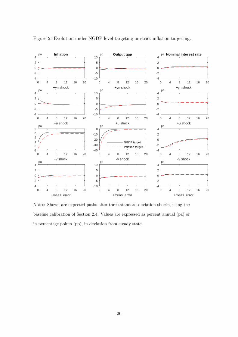
Figure 2: Evolution under NGDP level targeting or strict inflation targeting.

0 4 8 12 16 20

+yn shock

4

2

0

2

4Inflationpa

0 4 8 12 16 20

+yn shock

10

5

0

5

10Output gappp

0 4 8 12 16 20

+yn shock

4

2

0

2

4Nominal interest ratepa

0 4 8 12 16 20

+u shock

4

2

0

2

4pa

0 4 8 12 16 20

+u shock

10

5

0

5

10pp

0 4 8 12 16 20

+u shock

4

2

0

2

4pa

0 4 8 12 16 20

v shock

864202

pa

0 4 8 12 16 20

v shock

40

30

20

10

0pp

NGDP targetInflation target

0 4 8 12 16 20

v shock

4

2

0

2

4pa

0 4 8 12 16 20

+meas. error

4

2

0

2

4pa

0 4 8 12 16 20

+meas. error

10

5

0

5

10pp

0 4 8 12 16 20

+meas. error

4

2

0

2

4pa

Notes: Shown are expected paths after three-standard-deviation shocks, using the

baseline calibration of Section 2.4. Values are expressed as percent annual (pa) or

in percentage points (pp), in deviation from steady state.

26

Table 1: Economic performance under the optimal commitment policya

ZLB episodes Welfare lossb

Freq.c Durationd π x Tot.

No measurement error, no ZLB 0.0 0.0 0.01 0.02 0.03

Measurement error only 0.0 0.0 0.03 0.03 0.06

ZLB only 14.5 2.9 0.03 0.05 0.08

Measurement error and ZLB 11.3 3.1 0.05 0.06 0.11

a. Baseline calibration of Section 2.4.

b. Permanent consumption loss in percentage points.

c. Expected percent of the time at ZLB.

d. Expected number of consecutive quarters at ZLB.

27

Table 2: Performance of the monetary policy rulesa



No measurement error, no ZLB

Commitment 0.0 0.0 0.01 0.02 0.03

NGDP target 0.0 0.0 0.06 0.01 0.07

Inflation target 0.0 0.0 0.00 0.05 0.05

Taylor rule 0.0 0.0 0.21 0.25 0.46

Measurement error only

Commitment 0.0 0.0 0.03 0.03 0.06

NGDP target 0.0 0.0 0.07 0.02 0.09


Taylor rule 0.0 0.0 0.31 0.27 0.58

ZLB only

Commitment 14.5 2.9 0.03 0.05 0.08

NGDP target 6.2 1.7 0.09 0.10 0.19


Taylor rule 4.5 3.4 0.23 0.29 0.52

Measurement error and ZLB

Commitment 11.3 3.1 0.05 0.06 0.11

NGDP target 6.3 1.7 0.11 0.11 0.22


Taylor rule 3.8 3.4 0.33 0.32 0.65

a. Baseline calibration of Section 2.4.




28

Table 3: Performance of the rules, alternate calibrationsa



Larger technology shocks (σyn = 1)

Commitment 11.1 3.1 0.05 0.06 0.11

NGDP target 6.0 1.7 0.11 0.11 0.22


Taylor rule 3.7 3.3 0.33 0.32 0.65

More persistent technology shocks(ρyn = 0.9

)Commitment 11.4 3.0 0.05 0.06 0.11

NGDP target 5.9 1.7 0.11 0.11 0.22


Taylor rule 3.8 3.4 0.33 0.32 0.65

Larger mark-up shocks (σu = 0.0625)

Commitment 11.3 3.1 0.06 0.07 0.13

NGDP target 6.1 1.7 0.13 0.11 0.24


Taylor rule 3.7 3.3 0.39 0.33 0.72

More persistent mark-up shocks (ρu = 0.9)

Commitment 11.2 3.1 0.05 0.07 0.12

NGDP target 5.6 1.7 0.12 0.12 0.24


Taylor rule 4.6 3.6 0.40 0.34 0.74

a. With measurement error and ZLB in the model.




29

Table 4: Alternate calibrations continueda



Larger demand shocks (σv = 1)

Commitment 17.9 3.8 0.10 0.10 0.20

NGDP target 10.0 2.0 0.16 0.25 0.41


Taylor rule 7.6 3.9 0.42 0.55 0.97

More persistent demand shocks (ρv = 0.9)

Commitment 13.2 5.4 0.10 0.06 0.16

NGDP target 6.4 2.4 0.18 0.21 0.39


Taylor rule 5.7 3.7 0.37 0.42 0.79

Lower steady-state interest rate (r = 0.5)

Commitment 19.7 4.1 0.10 0.09 0.19

NGDP target 10.6 2.0 0.16 0.24 0.40


Taylor rule 10.4 4.3 0.38 0.42 0.80

a. With measurement error and ZLB in the model.




30

output gaps and robust monetary policy rules · output gaps and robust monetary policy rules...

Documents