FEDERAL RESERVE BANK OF SAN FRANCISCO

WORKING PAPER SERIES

Working Paper 2007-08 http://www.frbsf.org/publications/economics/papers/2006/wp07-08bk.pdf

The views in this paper are solely the responsibility of the authors and should not be interpreted as reflecting the views of the Federal Reserve Bank of San Francisco or the Board of Governors of the Federal Reserve System.

Robust Monetary Policy with Imperfect Knowledge

Athanasios Orphanides Board of Governors of the Federal Reserve System

John C. Williams

Federal Reserve Bank of San Francisco

March 2007

Robust Monetary Policy with Imperfect Knowledge

Athanasios OrphanidesBoard of Governors of the Federal Reserve System

andJohn C. Williams∗

Federal Reserve Bank of San Francisco

March 2007

Abstract

We examine the performance and robustness properties of monetary policy rules in anestimated macroeconomic model in which the economy undergoes structural change andwhere private agents and the central bank possess imperfect knowledge about the truestructure of the economy. Policymakers follow an interest rate rule aiming to maintainprice stability and to minimize fluctuations of unemployment around its natural rate but areuncertain about the economy’s natural rates of interest and unemployment and how privateagents form expectations. In particular, we consider two models of expectations formation:rational expectations and learning. We show that in this environment the ability to stabilizethe real side of the economy is significantly reduced relative to an economy under rationalexpectations with perfect knowledge. Furthermore, policies that would be optimal underperfect knowledge can perform very poorly if knowledge is imperfect. Efficient policies thattake account of private learning and misperceptions of natural rates call for greater policyinertia, a more aggressive response to inflation, and a smaller response to the perceivedunemployment gap than would be optimal if everyone had perfect knowledge of the economy.We show that such policies are quite robust to potential misspecification of private sectorlearning and the magnitude of variation in natural rates.

Keywords: Monetary policy, natural rate misperceptions, rational expectations, learning.

JEL Classification System: E52

Correspondence: Orphanides: Federal Reserve Board, Washington, D.C. 20551, Tel.: (202) 452-2654,e-mail: Athanasios.Orphanides@frb.gov. Williams: Federal Reserve Bank of San Francisco, 101Market Street, San Francisco, CA 94105, Tel.: (415) 974-2240, e-mail: John.C.Williams@sf.frb.org.∗We would like to thank Jim Bullard, Stephen Cecchetti, Alex Cukierman, Stephen Durlauf, Vitor

Gaspar, Stefano Eusepi, Bruce McGough, Ricardo Reis, and participants at numerous presentations

for useful discussions and comments. The opinions expressed are those of the authors and do not

necessarily reflect views of the Board of Governors of the Federal Reserve System or the management

of the Federal Reserve Bank of San Francisco.

1 Introduction

To paraphrase Clausewitz, monetary policy is conducted in a fog of uncertainty. Our

understanding of many key features of the macroeconomic landscape remains imperfect,

and the landscape itself evolves over time. As emphasized by McCallum (1988) and Taylor

(1993), a crucial requirement for a monetary policy rule is that its good performance be

robust to various forms of model misspecification. In this view, it is not enough for a

monetary policy rule to be optimal in one specific model, but instead it must be “stress

tested” in a variety of alternative model environments before one can conclude with any

confidence that the policy is likely to perform well in practice.1 In this paper, we examine

the performance and robustness of monetary policy rules in the context of fundamental

uncertainty related to the nature of expectations formation and structural change in the

economy. Our goal is to identify characteristics of policy rules that are robust to these types

of imperfect knowledge, as well as to identify those that are not.

The first form of uncertainty facing the policymaker that we consider relates to the way

in which agents form expectations. There is a growing literature that analyzes a variety of

alternative models of expectations formation. The key conclusion we take from our reading

of this literature is that there is a great deal of uncertainty regarding exactly how private ex-

pectations are formed. In particular, the standard assumption of rational expectations may

be overly restrictive for monetary policy analysis, especially in the context of an economy

undergoing structural change. But, the available evidence does not yet provide unequivocal

support for any other single model of expectations formation. Therefore, fundamental un-

certainty about the nature of expectations formation appears to be an unavoidable aspect

of the policy environment facing central banks face today.

In this paper, we consider two popular alternative models of private expectations for-

mation. Our approach can easily be extended to incorporate other alternative models of

expectations as well, but for reasons of tractability, we leave this for future research. One

1For past applications of this approach, see Levin, Wieland, and Williams (1999, 2003), who study thecharacteristics of monetary policy rules that are robust to model uncertainty related to macroeconomicdynamics.

1

model is rational expectations, which assumes that private agents know all the parameters

of the model and form expectations accordingly. This, of course, is the model used in much

of the recent monetary policy rule literature. The second model is perpetual learning, where

it is assumed that agents do not know the true parameters of the model, but instead con-

tinuously reestimate a forecasting model (see Sargent (1999) and Evans and Honkapohja

(2001) for expositions of this model). This form of learning represents a relatively modest,

and arguably realistic, deviation from rational expectations. An advantage of the perpetual

learning framework is that it allows varying degrees of deviations in expectations formation

relative to the rational expectations benchmark, which are characterized by variation in a

single model parameter. As shown in Orphanides and Williams (2004, 2005a, 2005b), per-

petual learning on the part of economic agents introduces an additional layer of interaction

between monetary policy, expectations, and economic outcomes.

The second source of uncertainty that we consider is unobserved structural change, which

we represent in the form of low-frequency variation in the natural rates of unemployment

and interest. The equilibrium of our model economy is described in terms of deviations

from these natural rates. In particular, the inflation rate is in part determined by the

unemployment gap, the deviation of the unemployment rate from its natural rate. Similarly,

the unemployment rate gap is determined in part by the real interest rate gap, the difference

between the real short-term interest rate and the real natural rate of interest. We assume

that the central bank does not observe the true values of the natural rates and, indeed, is

uncertain about the processes generating the natural rates.

Natural rate uncertainty presents a difficulty for policymakers who follow an interest

rate rule with the goal of maintaining price stability and minimizing fluctuations of un-

employment around its natural rate. With perfect knowledge of natural rates, the setting

of policy would ideally account for the evolution of the economy’s natural rates. But, if

policymakers do not know the values of the natural rates of interest and unemployment

when they make policy decisions, they must either rely on inherently imprecise real-time

estimates of these rates for setting the policy instrument, or, alternatively, eschew natural

2

rates altogether and follow a policy rule that does not respond to natural rate estimates.

The evidence suggests there exists considerable uncertainty regarding the natural rates

of unemployment and interest and ambiguity about how best to model and estimate natural

rates, even with the benefit of hindsight.2,3 Indeed, the measurement of the natural rate of

output has been a key issue in U.S. monetary policy debates in both the 1970s and 1990s, and

uncertainty about the natural rate of interest has been the topic of increasing discussion.

The evidence indicates that substantial misperceptions regarding the economy’s natural

rates may persist for some time, before their presence is recognized. In the meantime,

policy intended to be contractionary may actually inadvertently be overly expansionary,

and vice versa. Moreover, in an environment where the private sector is learning, the

learning process can interact with the policy errors and feed back to economic outcomes, as

pointed out Orphanides and Williams, (2004, 2005a, 2005b) and Gaspar, Smets and Vestin

(2006).

We examine the effects and policy implications of imperfect knowledge of expectations

formation and unknown time-varying natural rates using a quarterly model of the U.S. econ-

omy estimated over 1981–2004. We first consider the performance and robustness charac-

teristics of simple operational monetary policy rules under perfect and imperfect knowledge.

We then analyze the characteristics and performance of policy rules optimized taking into

account model uncertainty about expectations formation and natural rate uncertainty. We

approach this problem of optimal policy under uncertainty from Bayesian and Min-Max

perspectives and compare the results.

Our analysis yields several key findings. First, the scope for stabilization of the real

economy in our model with imperfect knowledge is significantly reduced relative to the

economy under perfect knowledge (where private agents and the central bank are assumed

2See, for instance, Staiger, Stock, and Watson (1997), and Orphanides and Williams (2002) for documen-tation of the difficulties associated with the measurement of the natural rate of unemployment and real-timeestimates of the unemployment gap; Orphanides and van Norden (2002), and van Norden (2002) for therelated problem regarding the output gap; and Laubach and Williams (2003), Orphanides and Williams(2002) and Clark and Kozicki (2005) for the errors in real-time estimates of the natural rate of interest.

3Our focus is on natural rate concepts as commonly used in policy models and practical policy discussions,which corresponds to those described by Friedman (1968). Our usage differs from that of Woodford (2003)and others, who mean by “natural rates” the outcomes that would obtain in the absence of nominal rigidities.

3

to know all features of the model). Second, monetary policies that would be optimal under

perfect knowledge can perform very poorly when knowledge is imperfect. Third, the optimal

Bayesian policy under uncertainty performs very well across all of our model specifications

and is therefore highly robust to the types of model uncertainty that we examine here. This

policy features greater policy inertia, a larger response to inflation, and a smaller response to

the perceived unemployment gap than would be optimal under perfect knowledge. Fourth,

the resulting optimal Bayesian and Min-Max policies are closely related to policies that

target the price level as opposed to the inflation rate, despite the fact that we assume that

the objective is to stabilize the inflation rate not the price level.

The remainder of the paper is organized as follows. Section II discusses the problems

for monetary policy caused by natural rate mismeasurement. Section III briefly describes

the estimated macro model. Section IV describes the class of monetary policy rules that we

study. Section V presents the models of expectations formation and natural rate estimation.

Section VI provides details on the simulation methodology. Section 7 analyzes monetary

policy under different models of expectations formation, but assuming constant natural

rates. Section 8 explores the joint effects of alternative models of expectations and time-

varying natural rates. Section 9 examines the optimal Bayesian and Min-Max policies.

Section 10 concludes.

2 Natural Rates, Misperceptions, and Policy Errors

We start our analysis with an illustration of some of the difficulties presented by the evo-

lution of the economy’s natural rates. To highlight the role of natural rate misperceptions

and the role of policy in propagating them in the economy, consider a generalization of the

simple policy rule proposed by Taylor (1993). Let it denote the short-term interest rate

employed as the policy instrument, (the federal funds rate in the Unites States), πt the rate

of inflation, and ut the rate of unemployment, all measured in quarter t. The classic Taylor

rule can then be expressed by

it = r∗t + πt−1 + θπ(πt−1 − π∗) + θu(ut−1 − u∗

t ), (1)

4

where π∗ is the policymaker’s inflation target and r∗t and u∗

t are the policymaker’s latest

estimates of the natural rates of interest and unemployment, based on information available

during period t. Note that in this formulation, we restrict attention to the operational

version of the Taylor rule recognizing that, as a result of reporting lags, the latest available

information about actual inflation and economic activity in period t regards the previous

period, t − 1. Note also that here we consider a variant of the Taylor rule that responds

to the unemployment gap instead of the output gap for our analysis, recognizing that the

two are related by Okun’s (1962) law.4 In his 1993 exposition, Taylor examined response

parameters equal to 1/2 for both the inflation gap and the output gap. Using an Okun’s

coefficient of 2, this corresponds to setting θπ = 0.5 and θu = −1.0.

The Taylor rule has been found to perform quite well in terms of stabilizing economic

fluctuations, at least when the natural rates of interest and unemployment are accurately

measured.5 However, historical experience suggests that policy guidance from this family

of rules may be rather sensitive to misperceptions regarding the natural rates of interest

and unemployment. The experience of the 1970s, discussed in Orphanides (2003b) and

Orphanides and Williams (2005b), offers a particularly stark illustration of policy errors

that may result.6

Following Orphanides and Williams (2002), we explore two dimensions along which the

Taylor rule has been generalized that in combination offer the potential to mitigate the

problem of natural rate mismeasurement. The first aims to mitigate the effects of mismea-

surement of the natural rate of unemployment by partially (or even fully) replacing the

response to the unemployment gap with one to the change in the unemployment rate.7 The

second dimension we explore is incorporation of policy inertia, represented by the presence

of the lagged short-term interest rate in the policy rule. Policy rules that exhibit a sub-

4In what follows, we assume that an Okun’s law coefficient of 2 is appropriate for mapping the output gapto the unemployment gap. This is significantly lower that Okun’s original suggestion of about 3.3. Recentviews, as reflected in the work by various authors place this coefficient in the 2 to 3 range.

5See, e.g. the contributions in Taylor (1999a), which are also reviewed in Taylor (1999b).6See also Bullard and Eusepi (2005), Cukierman and Lippi (2005), and Collard and Dellas (2004).7This parallels a modification of the Taylor rule suggested by numerous researchers who have argued in

favor of policy rules that respond to the growth rate of output rather than the output gap when real-timeestimates of the natural rate of output are prone to measurement error. See, in particular, McCallum (2001),Orphanides (2003a, 2003b), Orphanides et al. (2000), Walsh (2003), and Leitemo and Lonning (2006).

5

stantial degree of inertia typically improve the stabilization performance of the Taylor rule

in forward-looking models.8 As argued by Orphanides and Williams (2002), the presence

of inertia in the policy rule also reduces the influence of the estimate of the natural rate

of interest on the current setting of monetary policy and, therefore, the extent to which

misperceptions regarding the natural rate of interest affect policy decisions. To see this,

consider the generalized Taylor rule of the form

it = θiit−1 + (1 − θi)(r∗

t + πt−1) + θπ(πt−1 − π∗) + θu(ut−1 − u∗

t ) + θ∆u(ut−1 − ut−2). (2)

The degree of policy inertia is measured by θi ≥ 0; cases where 0 < θi < 1 are fre-

quently referred to as “partial adjustment”; the case of θi = 1 is termed a “difference rule”

or “derivative control” (Phillips 1954), whereas θi > 1 represents superinertial behavior

(Rotemberg and Woodford, 1999). These rules nest the classic Taylor rule as the special

case when θi = θ∆u = 0.9

To see more clearly how misperceptions regarding the natural rates of unemployment

and interest translate to policy errors it is useful to distinguish the real-time estimates of

the natural rates, u∗

t and r∗t , available to policymakers when policy decisions are made, from

their “true” values u∗ and r∗. If policy follows the generalized rule given by equation (2),

then the “policy error” introduced in period t by misperceptions in period t is given by

(1 − θi)(r∗

t − r∗) + θu(u∗

t − u∗

t ).

Although unintentional, these errors could subsequently induce undesirable fluctuations

in the economy, worsening stabilization performance. The extent to which misperceptions

regarding the natural rates translate into policy induced fluctuations depends on the param-

eters of the policy rule. As is evident from the expression above, policies that are relatively

unresponsive to real-time assessments of the unemployment gap, that is those with small θu,

8See e.g. Levin et al. (1999, 2003), Rotemberg and Woodford (1999), Williams (2003), and Woodford(2003).

9Policy rules that allow for a response to the lagged instrument and the change in the output gap orunemployment rate have been found to offer a simple characterization of historical monetary policy inthe United States for the past few decades in earlier studies, e.g. Orphanides and Williams (2005b) andOrphanides (2003c).

6

minimize the impact of misperceptions regarding the natural rate of unemployment. Simi-

larly, inertial policies with θi near unity reduce the direct effect of misperceptions regarding

the natural rate of interest. That said, inertial policies also carry forward the effects of past

misperceptions of the natural rates of interest and unemployment on policy, and one must

take account of this interaction in designing policies robust to natural rate mismeasurement.

A limiting case that is immune to natural rate mismeasurement of the kind considered

here is a “difference” rule, in which θi = 1 and θu = 0:

it = it−1 + θπ(πt − π∗) + θ∆u(ut − ut−1). (3)

As Orphanides and Williams (2002) point out, this policy rule is as simple, in terms of the

number of parameters, as the original formulation of the Taylor rule and is arguably simpler

to implement in practice since it does not require knowledge of the natural rates of interest

or unemployment. However, because this type of rule ignores potentially useful information

about the natural rates of interest and unemployment, its performance relative to the classic

“level” Taylor rule and the generalized rule will depend on the degree of mismeasurement

and the structure of the model economy, as we explore below.

3 An Estimated Model of the U.S. Economy

We examine the interaction of natural rate misperceptions, learning, and expectations for

the design of robust monetary policy rules using a simple quarterly model motivated by the

recent literature on micro-founded models incorporating some inertia in inflation and output

(see Woodford, 2003, for a fuller discussion). The specification of the model is closely related

to that in Gianonni and Woodford (2005), Smets (2003), and others. The key difference

is that instead of the output gap concept in these models, we employ the unemployment

gap concept as the cyclical measure of real economic activity. As already noted, the two

concepts are closely related in practice by Okun’s law and the properties of the model are

largely invariant to this choice. In addition, the empirical problem of measuring the natural

rate of unemployment—needed to define the unemployment gap—is essentially similar to

the problem of measuring the level of potential output—needed to define the output gap.

7

3.1 The Structural Model

The model consists of the following two structural equations:

πt = φππet+1 + (1 − φπ)πt−1 + απ(ut − u∗

t ) + eπ,t, eπ ∼ iid(0, σ2eπ

), (4)

ut = φuuet+1 + (1 − φu)ut−1 + αu (re

t − r∗) + eu,t, eu ∼ iid(0, σ2eu

), (5)

where π denotes inflation, u denotes the unemployment rate, u∗ denotes the true natural

rate of unemployment, r denotes the ex ante short-term real interest rate and r∗ the natural

real rate of interest.

The “Phillips curve” in this model (equation 4) relates inflation (measured as the an-

nualized percent change in the GNP or GDP price index, depending on the period) during

quarter t to lagged inflation, expected future inflation, and the unemployment gap during

the current quarter. The parameter φπ measures the importance of expected inflation on

the determination of inflation, while (1−φπ) captures inflation inertia. The unemployment

equation (equation 5) relates the unemployment rate during quarter t to the expected future

unemployment rate and one lag of the unemployment rate and the ex ante real interest rate

gap.

We imposed the coefficients φπ = φu = 0.5 on the lead-lag structure of the two equations.

We opted to concentrate attention on this case to ensure that expectations are of comparable

importance for the determination of the rates of inflation and unemployment in the model.

These values for φπ and φu are the largest allowable by the micro-founded theory developed

in Woodford (2003) and are consistent with the empirical findings of Giannoni and Woodford

(2005) and others.10 To estimate the remaining parameters, as in Orphanides and Williams

(2002), we rely on survey forecasts as proxies for the expectations variable which allows

estimation of equations (4) and (5) with ordinary least squares. Specifically, we use the

mean values of the forecasts provided in the Survey of Professional Forecasters. From this

survey, we use the forecasts of the unemployment rate and three-month treasury bill rate as

10We note that in the specification shown in equations (4) and (5), the data do not reject the value 0.5for either φπ or φu. The unrestricted point estimate of φπ is in fact close to 0.5. However the unrestrictedestimate of φu is noticeably lower.

8

reported. For inflation, we rely on the annualized log difference of the GNP or GDP price

deflator, which we construct from the forecasts of real and nominal GNP or GDP which

are reported in the survey. We posit that the relevant expectations are those formed in

the previous quarter; that is, we assume that the expectations determining πt and ut are

those collected in quarter t− 1. This matches the informational structure in the theoretical

models (see Woodford, 2003, and Giannoni and Woodford, 2005). To match the inflation

and unemployment data as best as possible with these forecasts, we use first announced

estimates of these series. Our primary sources for these data are the Real-Time Dataset for

Macroeconomists and the Survey of Professional Forecasters, both currently maintained by

the Federal Reserve Bank of Philadelphia (Zarnowitz and Braun (1993), Croushore (1993)

and Croushore and Stark (2001)). For the estimation of the inflation equation, we also use

the most recent estimates of the NAIRU by the Congressional Budget Office (2001, 2002)

as a proxy of the true level of the historical natural rate of unemployment.

We obtain the following OLS estimates for our model between 1981:4 and 2004:2, where

the starting point of this sample reflects the availability of the Survey of Professional Fore-

casters data for the short-term interest rate.

πt = 0.5πet+1 + 0.5πt−1 − 0.192

(0.084)

(uet − u∗

t ) + eπ,t, σeπ= 1.11, DW = 2.00, (6)

ut = 0.5uet+1 + 0.5ut−1 + 0.036

(0.017)

(ret − r∗) + eu,t, σeu

= 0.29, DW = 0.84, (7)

The numbers in parentheses are the estimated standard errors of the corresponding regres-

sion coefficients. The estimated unemployment equation also includes a constant term that

provides an estimate of the natural real interest rate, which is assumed to constant in es-

timating this equation. The estimated residuals show no signs of serial correlation in the

price equation. Some serial correlation is suggested by the residuals of the unemployment

equation, but for simplicity we ignore this serial correlation in evaluating the performance

of monetary policies.

9

We model the natural rates as exogenous AR(1) processes independent of all other

variables. We assume these processes are stationary based on the finding using the standard

ADF test that one can reject the null of nonstationarity of both the unemployment rate and

real federal funds rate over 1950–2003 at the 5 percent level. However to capture the near-

nonstationarity of the series, we set the AR(1) coefficient to 0.99 and and then calibrate the

innovation variances to be consistent with estimates of time variation in the natural rates

in postwar U.S. data. In particular, we set the innovation standard deviation of the natural

rate of unemployment to 0.07 and that of the natural rate of interest to 0.085. These values

imply an unconditional standard deviation of the natural rate of unemployment (interest)

of 0.50 (0.60), in the low end of the range of standard deviations of smoothed estimates of

these natural rates suggested by various estimation methods (see Orphanides and Williams

2002 for details).

4 Monetary Policy

We evaluate the performance of monetary policies rules using a loss equal to the weighted

sum of the unconditional variances of the inflation rate, the unemployment gap, and the

change in the nominal federal funds rate:

L = V ar(π − π∗) + λV ar(u − u∗) + νV ar(∆(i)), (8)

where V ar(x) denotes the unconditional variance of variable x.11 We assume an inflation

target of zero percent. As a benchmark for our analysis, we assume λ = 4 and ν = 0.25.

Based on an Okun’s gap type relationship, the variance of the unemployment gap is about

1/4 that of the output gap, so this choice of λ corresponds to equal weights on inflation and

output gap variability. We consider the sensitivity of our results to alternative specifications.

We complete the structural model by specifying a monetary policy rule according to

11Taken literally, the structural model implies a second-order approximation to consumer welfare that isrelated to the weighted and discounted sum of expected variances of the quasi-difference of the inflation rateand the level and quasi-difference of the unemployment gap. For the present purposes, we use a standardspecification of the loss used in much of the monetary policy evaluation literature.

10

which the federal funds rate is determined by a generalized Taylor Rule of the form:

it = θiit−1 + (1 − θi)(r∗

t + πt−1) + θπ(πt−1 − π∗) + θu(ut−1 − u∗

t ) + θ∆u(ut−1 − ut−2), (9)

where r∗t−1 is the policymaker’s real-time estimate of the natural rate of interest and u∗

t is

the real-time estimate of the natural rate of unemployment. We describe the policymaker’s

estimation of natural rates in the next section. As mentioned earlier, we used lagged data

in the policy rule reflecting the lag in data releases.12 We focus on this class of four-

parameter monetary policy rules because further increases in the number of terms in the

policy the rule yield relatively small reductions in the central bank loss. In particular,

under rational expectations, the optimized four-parameter rule nearly replicates the first-

best optimal policy when natural rates are known and constant.

In the following we focus on different versions of this policy rule. In one, all four

parameters are freely chosen. We also examine the two alternative simpler, 2-parameter

rules that are nested by the generalized rule: The “level” variant, where we constrain θi

and θ∆u to be zero, and which is closer to the original Taylor rule; and the “difference”

variant, where we impose the constraints θi = 1 and θu = 0.

5 Expectations

We consider two methods by which private agents form expectations: rational expectations

and learning. Under rational expectations, private agents know all features of the model,

including the realized values of the natural rates. Under learning, we assume that private

agents form expectations using an estimated forecasting model, and that the central bank

forms estimates of the natural rates of interest and unemployment using simple time-series

methods. Specifically, following Orphanides and Williams (2005c), we posit that private

agents and central banks engage in perpetual learning, that is they reestimate their re-

spective models using a constant-gain least squares algorithm that weighs recent data more

12In Orphanides and Williams (2007), we also explore alternative operational variants of the Taylor rulethat are based on forecasts of inflation and economic activity and show that the basic thrust of the resultspresented here also applies to forecast-based policies.

11

heavily than past data.13 In this way, these estimates allow for the possible presence of

time variation in the economy, including in the natural rates of interest and unemployment.

Given the structure of the model, private agents need to forecast inflation, the unemploy-

ment rate, and the federal funds rate for up to two quarters into the future.

5.1 Perpetual Learning with Least Squares

Under perfect knowledge with no shocks to the natural rate of unemployment, the pre-

dictable components of inflation, the unemployment rate, and the interest rate in the model

each depend on a constant, one lag each of the inflation and the ex post real interest rate

(the difference between the nominal interest rate and the inflation rate), and one or two

two lags of the unemployment rate, depending on whether the policy rule responds to just

the lagged unemployment gap or also the change in the unemployment rate. We assume

that agents estimate forecasting equations for the three variables using a restricted VAR of

the form corresponding to the reduced form of the rational expectations (RE) equilibrium

with constant natural rates. They then construct multi-period forecasts from the estimated

VAR.

Consider the case where policy is described by the Taylor rule. To fix notation, let

Yt denote the 1 × 3 vector consisting of the inflation rate, the unemployment rate, and

the interest rate, each measured at time t: Yt = (πt, ut, it); let Xt be the 5 × 1 vector of

regressors in the forecast model: Xt = (1, πt−1, ut−1, it−1−πt−1); let ct be the 4×3 vector of

coefficients of the forecasting model. This corresponds to the case of the Taylor rule. In the

case of the generalized policy rule, the second lag of the unemployment rate also appears

in Xt.

Note that we impose that the forecasting model include only the variables that appear

with non-zero coefficients in the reduced form of the rational expectations solution of the

model with constant natural rates. In principle, these zero restrictions may help or hinder

the forecasting performance of agents in the model. In practice, allowing agents to include

13See also Sargent (1999), Cogley and Sargent (2001), Evans and Honkapohja (2001), Gaspar and Smets(2002), and Gaspar, Smets and Vestin (2006) for related treatments of learning.

12

additional lags of variables in the forecasting model worsens macroeconomic outcomes.

Thus, by imposing this structure, we are likely erring on the side of understating the costs

of learning on macroeconomic performance.

Using data through period t, the least squares regression parameters for the forecasting

model can be written in recursive form:

ct = ct−1 + κtR−1t Xt(Yt − X ′

tct−1), (10)

Rt = Rt−1 + κt(XtX′

t − Rt−1), (11)

where κt is the gain.

Under the assumption of least squares learning with infinite memory, κt = 1/t, as

t increases, κt converges to zero. Assuming constant natural rates, this mechanism will

converge to the correct expectations functions and the economy converges to the perfect

knowledge rational expectations equilibrium. That is, in our model the perceived law of

motion that agents employ for forecasting corresponds to the correct specification of the

equilibrium law of motion under rational expectations.

As noted above, to formalize perpetual learning we replace the decreasing gain implied

by the infinite memory recursion with a small constant gain, κ > 0.14 With imperfect

knowledge, expectations are based on the perceived law of motion of the inflation process,

governed by the perpetual learning algorithm described above.

5.2 Calibrating the Learning Rate

A key parameter for the constant-gain-learning algorithm is the updating rate κ. To cal-

ibrate the relevant range for this parameter we examined how well different values of κ

fit either the expectations data from the Survey of Professional Forecasters, following Or-

phanides and Williams (2005b). To examine the fit of the Survey of Professional Forecasters

(SPF), we generated a time series of forecasts using a recursively estimated VAR for the

inflation rate, the unemployment rate, and the federal funds rate. In each quarter we rees-

14In terms of forecasting performance, the “optimal” choice of κ depends on the relative variances of thetransitory and permanent shocks, as in the relationship between the Kalman gain and the signal-to-noiseratio in the case of the Kalman filter.

13

timated the model using all historical data available during that quarter (generally from

1948 through the most recent observation). We allowed for discounting of past observations

by using geometrically declining weights. This procedure resulted in reasonably accurate

forecasts of inflation and unemployment, with root mean squared errors (RMSE) compara-

ble to the residual standard errors from the estimated structural equations, (6) and (7). We

found that discounting past data with values corresponding to κ in the range 0.01 to 0.04

yielded forecasts closest on average to the SPF than the forecasts obtained with lower or

higher values of κ. In light of these results, we consider κ = 0.02 as a baseline value for our

simulations, but also examine the robustness of policies to alternative values of this param-

eter. The value κ = 0.02 is also in line with the discounting reported by Sheridan (2003)

as best for explaining the inflation expectations data reported in the Livingston Survey.

5.3 Policymaker’s estimation of natural rates

Given the time variation in the natural rates, policymakers need to continuously reestimate

these variables in real time. Based on the results of Williams (2005) who found that such a

procedure performed well and was reasonably robust to model misspecification, we assume

that policymakers use a simple constant gain method to update their natural rates based

on the observed rates of unemployment and ex post real interest rates. Thus, policymakers

update their estimates of the natural rates of unemployment and interest as follows:

r∗t = r∗t−1 + ζr(it−1 − πt−1 − r∗t−1), (12)

u∗

t = u∗

t−1 + ζu(ut−1 − u∗

t−1), (13)

where ζr and ζu are the updating parameters. We set ζr = ζu = ζ = 0.005; a lower value

would imply far longer history of usable data than we possess while a higher value reduces

natural rate estimate accuracy.

The model under imperfect knowledge consists of the structural equations for inflation,

the unemployment gap, the federal funds rate (the monetary policy rule), the forecasting

model, and the updating rule for the natural rates of interest and unemployment.

14

6 Simulation Methodology

As noted above, we measure the performance of alternative policies rules based on the

central bank loss equal to the weighted sum of unconditional variances of inflation, the

unemployment gap, and the change in the funds rate. In the case of rational expectations

with constant and known natural rates, we compute the unconditional variances numerically

as described in Levin, Wieland, and Williams (1999). In all other cases, we compute

approximations of the unconditional moments using stochastic simulations of the model.

6.1 Stochastic Simulations

For stochastic simulations, the initial conditions for each simulation are given by the rational

expectations equilibrium with known and constant natural rates. Specifically, all model

variables are initialized to their steady-state values, assumed without loss of generality to

be zero. The central bank’s initial perceived levels of the natural rates are set to their

true values, likewise equal to zero. Finally, the initial values of the c and R matrices

describing the private agents’ forecasting model are initialized to their respective values

corresponding to reduced-form of the rational equilibrium solution to he structural model

assuming constant and known natural rates.

Each period, innovations are generated from Gaussian distributions with variances re-

ported above. The innovations are assumed to be serially and contemporaneously uncor-

related. For each period, the structural model is simulated, the private agent’s forecasting

model is updated and a new set of forecasts computed, and the central bank’s natural rate

estimate is updated. We simulate the model for 41,000 periods and discard the first 1000

periods to mitigate the effects of initial conditions. We compute the unconditional mo-

ments from sample root mean squares from the remaining 40,000 periods (10,000 years) of

simulation data.

Private agents’ learning process injects a nonlinear structure into the model that may

generate explosive behavior in a stochastic simulation of sufficient length for some policy

rules that would do a good job of stabilizing the economy under rational expectations. One

15

possible cause of such explosive behavior is that the forecasting model itself may become

explosive. We take the view that in practice private forecasters reject explosive models.

We implement this by computing, in each period of the simulation, the maximum root of

the forecasting VAR excluding the constants. If this root falls below the critical value of

0.995, the forecast model is updated as described above; if not, we assume that the forecast

model is not updated and the matrices C and R are held at their respective previous period

values.15

This constraint on the forecasting model is insufficient to assure that the model economy

does not exhibit explosive behavior in all simulations. For this reason, we impose a second

condition that restrains explosive behavior. In particular, if the inflation rate, nominal

interest rate, or unemployment gap exceed in absolute value six times their respective un-

conditional standard deviations (computed under the assumption of rational expectations

and known and constant natural rates), then the variables that exceeds this bound is con-

strained to equal the corresponding limit in that period. These constraints on the model

are sufficient to avoid explosive behavior for the exercises that we consider in this paper and

are rarely invoked for most of the policy rules we study, particularly for optimized policy

rules. An illustrative example is the benchmark calibration of the model with monetary

policy given by the Taylor Rule with θπ = 0.5 and θu = −1, for which the limit on the

forecasting model is binding less than 0.1 percent of the time, and that on the endogenous

variables, only about 0.4 percent of the time.

7 Monetary Policy and Learning

We first consider the design of optimal monetary policy in the presence of learning by private

agents but assuming that natural rates are constant and known by the policymaker. In this

way we can more easily identify the private sector effects of learning in isolation. In the

next section, we analyze the case of private learning with time varying natural rates that

are unobserved by the policymaker.

15We chose this critical value so that the test would have a small effect on model simulation behaviorwhile eliminating explosive behavior in the forecasting model.

16

7.1 The Effects of Learning under the Taylor Rule

To gauge the effects of learning for a given monetary policy rule, we consider macroeconomic

performance under the Taylor Rule under alternative assumptions regarding the public’s

updating rate, κ. For these exercises, we assume that the policymaker knows the true

values of the natural rates of interest and unemployment and, consequently, does not face

the problem of natural rate misperceptions.

Table 1 reports the performance of the Taylor Rule given by θπ = 0.5 and θu = −1.0.

The coefficient on the unemployment gap has the reverse sign and is twice the size of the

coefficient of 0.5 on the output gap in the standard Taylor rule, the latter modification

reflecting the smaller variation in the unemployment gap relative to the output gap. The

first row shows the outcomes under rational expectations. (This can also be thought of

as corresponding to the limiting case κ = 0.) The second through fourth rows show the

outcomes under learning for values of κ ranging from 0.01 to 0.03 (recall that 0.02 is our

benchmark value).

The time variation in the coefficients of the forecasting model determining expectations

induces greater variability and persistence in inflation and the unemployment gap. As

shown in Table 1, the variability in these variables rises with the learning rate, κ, as does

their first-order unconditional autocorrelation.

In this model, the introduction of learning with constant natural rates induces nearly

proportional increases in the variability of inflation and the unemployment gap. For ex-

ample, in the case of κ = 0.02, the standard deviation of inflation is 32 percent higher

than under rational expectations, and that of the unemployment gap is 33 percent higher.

This holds true for other values of κ and stems from the fact that the model equations for

inflation and the unemployment rate have identical lead-lag structures. It is worth noting

that in other models, the two variables may be affected differently by learning.

The rise in persistence results from the effects of shocks on the estimated parameters

of the forecasting model. Consider, for example, a positive shock to inflation. Upon reesti-

mation of the forecasting model, a portion of the shock will pass through to the intercept

17

of the inflation forecasting equation. This raises in the next period the value of expected

inflation, which boosts inflation, and so on. If by chance another positive shock arrives, the

estimated coefficient on lagged inflation in the forecasting model will be elevated, further

raising the persistence of inflation.

A key aspect of learning is that its effects are especially felt in episodes when particularly

large shocks or a series of positively correlated shocks occurs. Indeed, the model impulse

responses to i.i.d. shocks, evaluated at the steady state, are quantitatively little different

from those in the model under rational expectations. However, following an unusually large

shock or a sequence of shocks in the same direction, the nonlinear nature of the learning

process can have profound effects. The unconditional moments thus represent an average of

periods in which the behavior of the economy is approximately that described by the rational

expectations equilibrium and episodes in which expectations deviate significantly from that

implied by rational expectations. Such “problem” episodes contribute importantly to the

deterioration in macroeconomic performance reported in the table.

7.2 Optimized Taylor-style Rules

We now consider the optimal coefficients of the Taylor-style rule under different assumptions

regarding learning. As noted above, for this exercise we assume weights of 4 on unemploy-

ment gap variability and 0.25 on interest rate variability. Table 2 reports summary results.

The first two columns in the table report the optimized coefficients of the policy rules,

the third through fifth columns report the standard deviations of the target variables, and

the sixth column reports the associated loss, denoted by L∗. The final column reports the

loss under the policy rule optimized under rational expectations (RE), denoted by LRE ,

evaluated under the alternative specifications of learning.

As can be seen, the optimized Taylor-style rule under rational expectations performs

very poorly when the public in fact is learning. If policy is given by the optimal policy

assuming rational expectations, the loss under the benchmark value of κ = 0.02 is nearly 60

percent higher than under the optimized Taylor-style rule policy given in the third row of the

table. The problem with the policy rule coefficients chosen assuming rational expectations

18

is the relatively weak response to inflation. This mild response to inflation allows inflation

fluctuations to feed into inflation expectations and back to inflation, driving the standard

deviation of inflation to 2.8 percent for κ = 0.02.

A particular problem with the policy optimized assuming rational expectations is that

it allows the autocorrelation of inflation to rise considerably if agents engage in learning,

prolonging the response of inflation expectations to any shock. For example, under the op-

timal policy assuming rational expectations, the first-order autocorrelation of inflation rises

from 0.71 under rational expectations to 0.90 under learning with κ = 0.02. The efficient

policy response with learning responds more aggressively to inflation relative to the optimal

response under rational expectations. The stronger response to inflation dampens inflation

variability and lowers the autocorrelation of inflation. Indeed, focusing on the outcomes

under the optimal policies, the resulting autocorrelation of inflation is only modestly higher

under learning than it is under rational expectations. Together, these effects reduce damag-

ing fluctuations in the coefficients of agents’ forecasting model and ensure greater economic

stability.

8 Interaction of Learning and Time-varying Natural Rates

Having examined some of the policy implications of perpetual learning under the maintained

assumption that natural rates are known and constant, we now turn our attention to the

more general case that acknowledges the possible presence of time variation in the natural

rates of interest and unemployment. In terms of the model, we add innovations to the

natural rate equations, introduce the central bank’s real-time updating problem and keep

track of the way in which policymaker estimates of the natural rate influence the setting of

policy. The learning model of the agents remains the same as considered before.

8.1 The Effects of Learning and Natural Rate Variation

Table 3 summarizes the optimal policy responses and associated economic outcomes under

learning and time-varying natural rates when monetary policy follows the classic Taylor

rule. The rows corresponding to “s = 0” report the results where both natural rates are

19

assumed to be constant and known by the policymaker; these results are identical to those

reported in Table 1 and provide a point of reference for the results that incorporate time

variation in the natural rates. The rows corresponding to “s = 1” report the results for the

main calibration of the innovation variances. Finally, the rows under the heading “s = 2”

report the results associated with standard deviation of the natural rate innovations that

are twice as large. The layout of the table is the same as Table 1 except that we have added

columns reporting the standard deviations of natural rate misperceptions.

Under the benchmark calibration of the innovation variances and private sector learning,

the standard deviation of central bank misperceptions of the natural rate of unemployment

is 0.6 percentage points, while that of the natural rate of interest is about 1.1 percentage

points. With higher innovation variances given by s = 2, the standard deviation of misper-

ceptions of the natural rate of unemployment increases to about 1.0 percentage points, and

of the natural rate of interest rises to about 1.6 percentage points. In all cases, these mis-

perceptions are highly persistent, with first-order autocorrelation of about 0.99 (not shown

in the table).

Time varying natural rates inject serially correlated errors to the processes driving in-

flation, the unemployment rate, and the interest rate. The coefficients of private agents’

forecasting model only gradually adjust to changes in the natural rates. Moreover, policy-

makers themselves are unavoidably confused about the true level of natural rates and these

misperceptions feed back into the coefficient estimates of the agents’ forecasting model. As

a result, these shocks and the feedback through policy back into expectations cause a dete-

rioration in macroeconomic performance. For a given rate of learning, the inclusion of time

varying natural rates affects the standard deviations of inflation and the unemployment gap

in about the same proportion. The introduction of time-varying natural rates also raises the

autocorrelations of inflation and the unemployment rate gap, as seen in the final columns

of Table 3.

To assess how policymakers would wish to adjust policy under alternative assumptions

regarding learning and natural rate variation, Table 4 reports the optimized Taylor-style

20

rules under the various alternatives. The format of the table parallels that of Tables 2

and 3. For comparison, the case of constant natural rates reported in Table 2 is provided

in the rows corresponding to s = 0.

As can be seen in the table, for a given rate of learning, time variation in natural rates

raises the optimal policy response to inflation and lowers that to the perceived unemploy-

ment gap. For example, for κ = 0.02, the optimal coefficient on inflation rises from 0.77

to 1.08 to 1.24 for s = 0, 1, and 2, respectively, and that on the unemployment gap falls

from 1.20 to 0.99 to 0.60 (in absolute value). The performance of the RE-optimal Taylor-

style rule, given in the final column, is truly abysmal in the model under learning and

time-varying natural rates.

Interestingly, for a given positive natural rate innovation variance, the optimal coeffi-

cients both on inflation and the unemployment gap are generally higher the greater is κ.

With time-varying natural rates but a low rate of learning, the optimal policy is to dampen

the response to the mismeasured unemployment gap and to concentrate on inflation. In this

case, expectations help stabilize the unemployment gap even with a modest direct policy

response to the gap, as discussed in Orphanides and Williams (2002). But, with a higher

rate of learning, noise in the economy, including that related to time-varying natural rates,

interferes with the public’s understanding of the economy and expectations formation may

no longer act as a stabilizing influence. In these circumstances, policy needs to respond rela-

tively strongly to the perceived unemployment gap, even recognizing that this may amplify

policy errors owing to natural rate misperceptions. Doing so helps stabilize unemployment

expectations and avoids situations where private expectations of unemployment veer away

from fundamentals.

Figure 1 presents a graphical perspective on the performance of the economy correspond-

ing to alternative rules under the various possibilities regarding the degree of time-variation

in natural rates and rate of learning. In the figure, each panel shows iso-loss contours drawn

from the loss associated with policies for alternative parameters θπ and θu, as shown in the

two axes. The top left panel shows the loss associated with these policies under rational

21

expectations and constant natural rates. The remaining panels show the loss under ratio-

nal expectations or under learning for different degrees of variation in the natural rates,

s = {0, 1, 2}. Each panel corresponds to one of the 12 possible alternative combinations of

these assumptions—comparable to the alternatives in Table 4. The minimum loss achiev-

able with a Taylor rule under the assumptions in each panel is also identified. Comparing

these points across the different panels shows how the optimal response coefficients of the

Taylor rule vary with the alternative assumptions. The figure also allows examination of

the loss associated with a specific policy that may be optimal under one set of assump-

tions when implemented in an economy where an alternative set of assumptions hold. This

provides a useful graphical overview of the robustness characteristics of alternative rules.

Of particular interest in this regard is an important asymmetry pertaining to the robust-

ness characteristics of the responsiveness to inflation in the Taylor rule. While the loss

across alternative assumptions is extremely sensitive to changes in θπ when that is near

the RE-optimal policy, a similar sensitivity is not evident for the higher values of θπ that

are optimal under learning. This suggests that robust Taylor rule policies may need to be

considerably more aggressive towards inflation compared to the RE-optimal policies. We

return to a detailed examination of the design of robust rules later on.

8.2 Optimized Difference Rule

The Taylor-style rule implicitly places a coefficients of one on the perceived natural rate of

interest and −θu on the perceived unemployment gap. As discussed in Orphanides et al

(2000) and Orphanides and Williams (2002) in forward-looking models with natural rate

misperceptions, an alternative specification of a policy rule that does not respond directly

to perceived natural rates may perform better than the Taylor-style rule specification. In

light of that, we consider one such specification of a two-parameter policy rule in which

θi is constrained to equal one, θu is constrained to equal zero, and θπ and θ∆u are freely

chosen to minimize the policymaker loss. We refer to policy rules with this specification

as “difference” rules. Because the policy rule responds to the lagged first-difference of the

unemployment rate, we expand private agents’ forecasting model to include the second

22

lag on the unemployment rate. With this specification, the learning model is identical to

the reduced form rational expectations solution of the model with constant natural rates.

Table 5 summarizes the results from rules of this optimized to the 12 alternative sets of

assumptions regarding the formation of expectation and variation in natural rates. The

losses resulting under the optimized difference rules are reported in the sixth column under

the heading L∗

D; for comparison, the loss under the optimized Taylor-style rule is given

in the final column of the table. Figure 2 presents contour plots of these rules under the

alternative assumptions, in a format directly comparable to that of Figure 1, except that

θ∆u rather than θu is plotted on the vertical axis.

As can be seen in the table, with time-varying natural rates, the optimized first-difference

rules outperform the optimized Taylor-style rules. The more volatile the natural rates are,

the greater the performance advantage of the difference rules over the Taylor-style rules.

With constant natural rates, the Taylor-style rules perform better than the difference rules,

reflecting the fact that when policymakers have perfect knowledge of the natural rates of

interest and unemployment, it pays to use this information in the setting of policy. We

conclude that in an environment of imperfect knowledge, difference rules may provide a

better simple benchmark for policy than level Taylor-style rules.

As in the case of the Taylor-style rule, both the existence of private sector learning

and time variation in natural rates imply stronger optimal responses to inflation relative

to rational expectations. The optimal coefficient on the change in the unemployment rate,

however, is relatively insensitive to the learning rate and the degree of natural rate variation.

In addition, as can be seen from the figure, in all panels the loss function appears to be

relatively flat in the region around the optimal difference rule for our benchmark case with

learning (s = 1 and κ = 0.02), suggesting that a benchmark difference rule can be selected

that would be robust to uncertainty regarding the precise degree of time-variation in natural

rates and expectations formation mechanism.

23

8.3 Optimized Generalized Rules

Next, we consider the performance of the generalized form of the policy rule that combines

elements of both the Taylor rule and the difference rule studied above. The specification,

shown in equation (9), is the same as in Orphanides and Williams (2002). Here, the interest

rate depends on the lagged interest rate, the lagged inflation rate and perceived unemploy-

ment gap, and the lagged changed in the unemployment rate. Optimal rules for each of

the twelve combinations of alternative assumptions regarding learning and natural rates are

shown in Table 6. In the table, which follows the same general structure as Tables 4 and 5,

the loss from the optimal generalized policy rule is denoted by L∗

4; for comparison, the loss

resulting from the optimized difference rule, denoted by L∗

D, and the optimized Taylor-style

rule, denoted by L∗

2, are reported in the final two columns of the table.

The optimized four-parameter rules perform significantly better than the optimized

Taylor-style rules, especially in the presence of time varying natural rates, and outperforms

the simple difference rule, particularly when natural rates are constant. This superior

performance is related to three factors. First, rules in this class respond to more vari-

ablesinformation, in particular the lagged funds rate, and thus have an advantage over the

simple Taylor rule. Second, by incorporating a near-unity response to the lagged funds

rate, the optimal generalized rules nearly completely remove the perceived natural rate of

interest from influencing policy. Movements in the true natural rate of interest affect the

economy, but there is no direct feedback of central bank misperceptions of the natural rate

of interest to the economy. Third, by responding to the change in the unemployment rate

as a proxy for the unemployment gap, this specification allows for a strong response to

utilization variables without relying exclusively on imperfect measures of the gap.

9 Robust Policy

A striking feature of the results from the generalized policy rule is that the optimal coeffi-

cients of the rule do not appear to be very sensitive to the rates of learning that we consider

or the magnitude of variation in natural rates, as long as both elements are present. In

24

all cases, the optimal coefficient on the lagged funds rate is near one. The coefficients on

inflation and the unemployment gap vary, but are generally of approximately the same size.

And the coefficient on the change in the unemployment rate is relatively similar across

the different cases. These findings suggest that precise knowledge regarding the extent of

imperfections in the formation of expectations or extent of natural-rate variation may not

be crucial for designing a good policy rule. What is more critical is to acknowledge these

imperfections in the design of the rule.

To highlight the concern for robustness, Figures 3 and 4 present a graphical summary

of alternative simulations that quantify the costs of pursuing policy optimized under poten-

tially incorrect assumptions. In Figure 3 we examine the problem arising from potentially

incorrect assumptions regarding the extent of variation in natural rates. To isolate this com-

plication, we maintain that expectations are rational and plot the outcomes corresponding

to the generalized policy rules optimized for s = {0, 1, 2}.16 (The parameters of these rules

are shown in the first three rows of Table 6). As can be seen, the performance of the rule

optimized under perfect knowledge is truly abysmal for even small degrees of time-variation,

whereas, the performance of the rules optimized for s = 1 and s = 2 is relatively insensitive

to the true degree of variation in natural rates.

Similarly, in Figure 4 we examine the problem arising from potentially incorrect assump-

tions regarding the formation of expectations. To illustrate this complication in isolation,

we maintain s = 0 and plot the outcomes corresponding to the generalized policy rules

optimized for κ = {0, 0.01, 0.02}. (The parameters of these rules are shown in rows 1, 4

and 7 in Table 6). Here as well, we see that the performance of the rule optimized on the

assumption that expectations are rational (denoted with κ = 0 here) deteriorates rapidly

as the true value of κ increases, and is quite poor even when κ is much smaller than our

benchmark value of 0.02. By contrast, the performance of the rules optimized for either

κ = 0.01 or κ = 0.02 is much less sensitive to the true value and the loss is smaller than

16With the maintained assumption of rational expectations, this experiment follows that reported inOrphanides and Williams (2002) concerning unknown natural rates and provides confirmation of the resultsreported there.

25

that of the RE-optimal rule for any values of κ larger than 0.005.

As the experiments described above demonstrate, failing to account for imperfect knowl-

edge can be costly in both of the dimensions of uncertainty we consider. The challenge is

to design a policy rule that would be robust to all recognized sources of uncertainty. To

that end, we turn to an examination of robustness of a benchmark policy following the

methodology in Levin, Wieland, and Williams (2003). An informative benchmark rule may

be identified with the optimal policy rule corresponding to an agnostic Bayesian prior when

the policymaker does not know which among a range of models is a better representation

of the economy. For our benchmark, we assume that the policymaker is unsure about both

the degree of structural change in the economy, as reflected in variation in natural rates,

as well as about how expectations are formed, that is whether they are rational or based

on adaptive learning. Thus, we assume the policymaker has a flat prior on three possible

values of s = {0, 1, 2}), and on four possible models for expectations, rational and learning

with values κ = {0.01, 0.02, 0.03}. The policymaker’s objective, then, is to identify the

policy rule (8) that minimizes the expected loss (9) accounting for his agnostic prior over

the correct model. Note that since he is uncertain about the presence of structural change,

the policymaker updates his estimates of natural rates using his updating rules (12) and

(13) to set policy.

The optimal Bayesian policy for our baseline loss (λ = 4 and ν = 0.25) is:

it = 0.96it−1 + (1− 0.96)(r∗t + πt−1)+ 0.69(πt−1 −π∗)− 0.75(ut−1 − u∗

t )− 2.57(ut−1 −ut−2).

Note that this is rather similar to the optimal policy corresponding to the optimized rule for

κ = 0.02 and s = 1 reported in Table 6. Table 7 reports the performance of the economy

when this benchmark policy rule is followed for the various alternative specifications of

expectations formation and natural rate variation. The last two columns present a summary

comparison. The fifth column LB4 , reports the loss associated with the specification listed in

he first column when the optimal Bayesian rule is followed. The last column, L∗

4 reports the

best-obtainable loss from a four-parameter rule optimized to that particular specification

of the model, as given in Table 6.

26

The benchmark Bayesian rule performs very well across all different combinations of

parameterizations of learning and natural rate fluctuations. In the parlance of Levin and

Williams (2003), the model is reasonably fault tolerant once policy has accounted for some

degree of learning and natural rate variation. The relative performance of this rule is

actually poorest in the cases of little or no learning and constant natural rates. But,

these are states of the world that are associated with the lowest loss so from a robustness

perspective, the loss in efficiency in such situations is less worrisome than the outcomes

corresponding to the larger losses that might occur under substantial variation in natural

rates and learning. Remarkably, the relative performance of the benchmark rule is excellent

for all values of κ for both s = 1 and s = 2.

Three of the parameters of the benchmark Bayesian rule differ noticeably from the RE-

optimal policy. First, the response of policy to inflation is considerably more aggressive.

Second, the rule is almost completely inertial, that is, θi is close to unity. Third the policy

responsiveness to changes in unemployment is larger, while that to the level of the estimated

unemployment gap is muted. To check the sensitivity of these findings to the assumption of

a flat prior over the twelve model specifications, we also repeated the Bayesian optimization

with alternative priors. The results suggested that the optimal Baysesian policy exhibited

these three differences relative to the RE-optimal policy for a wide range of alternatives

in our model. In particular these results held as long as the policymaker assigned some

non-trivial probability to the possibility that knowledge is imperfect.

An alternative way to design a robust policy is by identifying the optimal rule under a

Min-Max criterion. The Min-Max policy minimizes the maximum loss for the model under

the alternative assumptions under consideration which here occurs when κ and s take their

largest values, 0.03 and 2, respectively. The loss corresponding to this rule for the 12

alternative sets of assumptions is reported in the column labeled LM4 in Table 8. As can

be seen in the table, this rule does very well when κ and s are in the upper halves of their

respective allowable ranges, but not as well when these parameters are both in the lower

halves of the ranges. Indeed, in only two of the twelve cases of parameter combinations that

27

we consider does the Min-Max policy outperform the optimal Bayesian policy and even in

those cases the loss is only very modestly lower.

The analysis above was based on a baseline specification of the loss function, but we

are also interested in the sensitivity of robust-rule design to alternative weights. This is

of particular interest because, as with other aspects of the monetary policy problem, it

is not entirely clear what the appropriate relative weights on the stabilization of inflation

and employment should be. Recall that our baseline loss function has a unit weight on

inflation and a weight λ = 4 on unemployment variability (which corresponds to a unit

weight on output gap variability). In Table 9 we show the parameters of optimal rules

for alternative values of λ ranging from 0 to 16. For each specification, we compare the

parameters of the RE-optimal rule with the parameters of the optimal Bayesian and Min-

Max rules corresponding to the same preferences. Some key results are evident for all of the

relative stabilization weights. The robust rules exhibit a high degree of inertia and are much

more responsive to inflation than the corresponding RE-optimal policies. Indeed, with the

Min-Max criterion, the optimal rule is essentially a difference rule (θi = 1) and the robust

response to inflation is about 1 regardless of the weight in the loss functions. Relative to

the RE-optimal policies, the robust rules are much less responsive to the unemployment

gap and more responsive to changes in unemployment, but these parameters vary with the

relative weight in the loss function.

Finally, we wish to examine the robustness of simpler policies than the generalized rule

which has four parameters, as simpler rules, for example rules that only have one or two

argument, may be more useful than their more complicated counterparts in policy discus-

sions. To that end, we compute the optimal Bayesian and Min-Max level and difference

rules each of which has only two parameters. We report results for the baseline preferences

we consider, λ = 4 and ν = 0.25. For the Bayesian rules, we employ the same flat prior

over the alternative models of learning and natural rates as before. The resulting optimal

Bayesian rules are:

it = r∗t + πt−1 + 1.07(πt−1 − π∗) − 0.77(ut−1 − u∗

t )

28

it = it−1 + 0.65(πt−1 − π∗) − 4.12(ut−1 − ut−2).

The corresponding Min-Max rules are:

it = r∗t + πt−1 + 1.43(πt−1 − π∗) − 0.87(ut−1 − u∗

t )

it = it−1 + 0.95(πt−1 − π∗) − 4.60(ut−1 − ut−2).

Table 10 presents a summary comparison of the optimal two-parameter rules. The optimal

level rule performs uniformly worse than the optimal difference rule in this comparison.

Given a choice among these simple alternatives, the difference rule proves clearly more

robust in protecting against the uncertainties regarding expectations formation and natural

rates. But, as can be seen by comparing the loss to those in Table 8, the generalized rule

with its added flexibility delivers better performance, especially when s is small.

10 Conclusion

In an environment of imperfect knowledge regarding the potential for structural change in

the economy and the formation of expectations, the scope for stabilization of the real side

of our economy may be significantly reduced relative to an economy under rational expec-

tations with perfect knowledge. Policies that appear to be optimal under perfect knowledge

can perform very poorly if they are implemented in such an environment. In our model econ-

omy, the presence of imperfect knowledge tends to raise the persistence of inflation, partly

as a result of the persistent policy errors due to misperceptions of the natural rates and

partly as a result of the learning process agents may rely upon to form expectations. This

leads to a deterioration in economic performance, especially with regard to a policymaker’s

price stability objective. Policymakers who recognize the presence of these imperfections

in the economy can adjust their policies and protect against this deterioration in economic

outcomes.

Efficient policies that take account of private learning and misperceptions of natural rates

appear to have two important characteristics. First, and arguably most important, these

policies call for more aggressive responses to inflation that would be optimal under perfect

29

knowledge. This finding tends to confirm the conventional wisdom that associates good

central bank policy practice with policies that may appear to stress the role of maintaining

price stability more than might appear warranted in simple models of the economy under

perfect knowledge. Second, efficient policies exhibit a high degree of inertia in the setting

of the interest rate. Indeed, simple difference rules which circumvent the need to rely on

uncertain estimates of natural rates in setting policy, appear to be robust to potential

misspecification of private sector learning and the magnitude of variation in natural rates.

Importantly, it seems possible to design a simple policy rule that can deliver reasonably good

macroeconomic performance even in an environment of considerable uncertainty regarding

expectations formation and natural rate uncertainty.

30

References

Bullard, James and Stefano Eusepi (2005), “Did the Great Inflation Occur Despite Policy-maker Commitment to a Taylor Rule?” Review of Economic Dynamics, 8(2), 324-59.

Clark, Todd, and Sharon Kozicki (2005), “Estimating Equilibrium Interest Rates in RealTime,” North American Journal of Economics and Finance, 16(3), 395-413.

Cogley, Timothy and Sargent, Thomas (2001), “Evolving Post-World War II U.S. InflationDynamics,” in NBER Macroeconomics Annual.

Collard, Fabrice and Harris Dellas (2004), “The Great Inflation of the 1970s,” EuropeanCentral Bank Working Paper 336, April.

Congressional Budget Office (2001), “CBO’s Method for Estimating Potential Output: AnUpdate,” Washington, DC: Government Printing Office (August).

Congressional Budget Office (2002), The Budget and Economic Outlook: An Update. Wash-ington DC: Government Printing Office (August).

Croushore, Dean (1993), “Introducing: The Survey of Professional Forecasters,” FederalReserve Bank of Philadelphia Business Review, November/December, 3–13.

Croushore, Dean and Tom Stark (2001), ”A Real-Time Data Set for Macroeconomists,”Journal of Econometrics 105, 111–130, November.

Cukierman, Alex and Francesco Lippi (2005), “Endogenous Monetary Policy with Unob-served Potential Output,” Journal of Economic Dynamics and Control, 29(11), pp.1951-83.

Evans, George and Honkapohja, Seppo (2001), Learning and Expectations in Macroeco-

nomics. Princeton: Princeton University Press.

Friedman, Milton (1968), “The Role of Monetary Policy,” American Economic Review,58(1), 1-17.

Gaspar, Vitor and Smets, Frank (2002), “Monetary Policy, Price Stability and Output GapStabilisation,” International Finance, 5(2), Summer, 193–211.

Gaspar, Vitor, Frank Smets, and David Vestin (2006). “Adaptive Learning, Persistence,and Optimal Monetary Policy” ECB Working paper, June.

Giannoni, Marc P. and Michael Woodford (2005). “Optimal Inflation Targeting Rules,” inThe Inflation Targeting Debate, Ben Bernanke and Michael Woodford (eds.), Chicago:University of Chicago Press.

Laubach, Thomas and John C. Williams (2003). “Measuring the Natural Rate of Interest,”Review of Economics and Statistics, 85(4) 1063-1070.

Leitemo, Kai, and Ingunn Lonning (2006). “Simple Monetary Policymaking without theOutput Gap.” Journal of Money, Credit, and Banking 38(6), p. 1619-1640.

Levin, Andrew, Volker Wieland and John Williams (1999), “Robustness of Simple MonetaryPolicy Rules under Model Uncertainty,” in Monetary Policy Rules, John B. Taylor (ed.),Chicago: University of Chicago.

Levin, Andrew, Volker Wieland and John Williams (2003), “The Performance of Forecast-Based Policy Rules under Model Uncertainty,” American Economic Review, 93(3), 622–645, June.

31

McCallum, Bennett T. (1988). “Robustness Properties of a Rule for Monetary Policy.”Carnegie-Rochester Conference Series on Public Policy, 29, Autumn, 173-203.

McCallum, Bennett T. (2001). “Should Monetary Policy Respond Strongly to OutputGaps?” American Economic Association Papers and Proceedings, 91(2), May, 258-262.

Okun, Arthur (1962), “Potential Output: Its Measurement and Significance,” in Amer-

ican Statistical Association 1962 Proceedings of the Business and Economic Section,Washington, D.C.: American Statistical Association.

Orphanides, Athanasios (2003a), “Monetary Policy Evaluation With Noisy Information,”Journal of Monetary Economics, 50(3), 605-631, April.

Orphanides, Athanasios (2003b), “The Quest for Prosperity Without Inflation,” Journal of

Monetary Economics, 50(3), 633-663, April.

Orphanides, Athanasios (2003c), “Historical Monetary Policy Analysis and the TaylorRule,” Journal of Monetary Economics, 50(5), 983-1022, July.

Orphanides, Athanasios, Richard Porter, David Reifschneider, Robert Tetlow and FredericoFinan (2000), “Errors in the Measurement of the Output Gap and the Design of Mon-etary Policy,” Journal of Economics and Business, 52(1/2), 117-141, January/April.

Orphanides, Athanasios and Simon van Norden (2002), “The Unreliability of Output GapEstimates in Real Time,” Review of Economics and Statistics, 84(4), 569–583, Novem-ber.

Orphanides, Athanasios and John C. Williams (2002), “Robust Monetary Policy Rules withUnknown Natural Rates”, Brookings Papers on Economic Activity, 2:2002, 63-118.

Orphanides, Athanasios and John C. Williams (2005a), “Inflation scares and forecast-basedmonetary policy”, Review of Economic Dynamics, 8(2), 498-527, April.

Orphanides, Athanasios and John C. Williams (2005b), “The Decline of Activist Stabi-lization Policy: Natural Rate Misperceptions, Learning, and Expectations” Journal of

Economic Dynamics and Control. 29(11), 1927-1950, November.

Orphanides, Athanasios and John C. Williams (2005c) “Imperfect Knowledge, InflationExpectations and Monetary Policy,” in The Inflation Targeting Debate, Ben Bernankeand Michael Woodford (eds.), Chicago: University of Chicago Press.

Orphanides, Athanasios and John C. Williams (2007) “Inflation Targeting Under ImperfectKnowledge,” in Monetary Policy Under Inflation Targeting, Frederic Mishkin and KlausSchmidt-Hebbel (eds.), Santiago: Central Bank of Chile.

Phillips, A. W. (1954), “Stabilisation Policy in a Closed Economy,” Economic Journal,290–323, June.

Rotemberg, Julio J. and Michael Woodford (1999), “Interest Rate Rules in an EstimatedSticky Price Model,” in Monetary Policy Rules, John B. Taylor (ed.), Chicago: Univer-sity of Chicago Press, 57–119.

Sargent, Thomas J. (1999), The Conquest of American Inflation, Princeton: PrincetonUniversity Press.

Sheridan, Niamh (2003), “Forming Inflation Expectations,” Johns Hopkins University,mimeo, April.

32

Smets, Frank (2003), “Maintaining Price Stability: How Long Is the Medium Term?” Jour-

nal of Monetary Economics, September 2003, 50(6), 1293-1309.

Staiger, Douglas, James H. Stock, and Mark W. Watson (1997), “How Precise are Estimatesof the Natural rate of Unemployment?” in: Reducing Inflation: Motivation and Strategy,ed. by Christina D. Romer and David H. Romer, Chicago: University of Chicago Press.195-246.

Taylor, John B. (1993), “Discretion versus Policy Rules in Practice,” Carnegie-RochesterConference Series on Public Policy, 39, December, 195–214.

Taylor, John B., ed., (1999a), Monetary Policy Rules, Chicago: University of Chicago.

Taylor, John B. (1999b), “The Robustness and Efficiency of Monetary Policy Rules asGuidelines for Interest Rate Setting by the European Central Bank,” Journal of Mone-

tary Economics, 43(3), 655-679.

van Norden, Simon (2002), “Filtering for Current Analysis” Bank of Canada Working Paper2002-28, October.

Walsh, Carl (2003), “Implications of a Changing Economic Structure for the Strategy ofMonetary Policy,” in Monetary Policy and Uncertainty: Adapting to a Changing Econ-

omy, Federal Reserve Bank of Kansas City.

Williams, John C. (2003) “Simple Rules for Monetary Policy,” Federal Reserve Bank of San

Francisco Review, 1-12.

Williams, John C. (2005). “Robust Estimation and Monetary Policy with UnobservedStructural Change.” In Models and Monetary Policy: Research in the Tradition of

Dale Henderson, Richard Porter and Peter Tinsley, edited by Jon Faust, AthanasiosOrphanides and David L. Reifschneider. Washington: Board of Governors of the FederalReserve System.

Woodford, Michael (2003), Interest and Prices: Foundations of a Theory of Monetary Pol-

icy, Princeton University Press.

Zarnowitz, Victor and Phillip A. Braun (1993), “Twenty-two Years of the NBER-ASAQuarterly Economic Outlook Surveys: Aspects and Comparisons of Forecasting Perfor-mance,” in Business Cycles, Indicators, and Forecasting, James H. Stock and Mark W.Watson (eds.), Chicago: University of Chicago Press, 11–84.

33

Table 1Performance of the Taylor Rule with Learning

(constant natural rates)

First-orderStandard Deviation Autocorrelation

κ π u − u∗ ∆i π u − u∗ i

RE 1.48 0.54 1.96 0.64 0.77 0.600.01 1.68 0.63 1.97 0.72 0.83 0.670.02 1.95 0.72 1.99 0.79 0.86 0.750.03 2.13 0.79 2.03 0.81 0.88 0.78

Notes: it = r∗t + πt−1 + 0.5 × (πt−1 − π∗) − 1 × (ut−1 − u∗

t )

34

Table 2Optimized Taylor-style Rule with Learning

(constant natural rates)

Policy Rule Standard First-orderCoefficient Deviation Autocorrelation Loss

κ π u − u∗ π u − u∗ ∆i π u − u∗ L∗ LRE

RE 0.16 −1.38 1.60 0.47 1.53 0.71 0.75 4.0 4.00.01 0.53 −1.21 1.69 0.61 2.02 0.73 0.82 5.4 7.00.02 0.77 −1.20 1.73 0.72 2.34 0.74 0.85 6.4 10.30.03 0.89 −1.37 1.81 0.77 2.53 0.75 0.86 7.3 12.4

Notes: it = r∗t + πt−1 + θπ(πt−1 − π∗) + θu(ut−1 − u∗

t )

35

Table 3The Taylor Rule with Learning

(time-varying natural rates)

Standard First-orderDeviation Autocorrelation

s π u − u∗ ∆i u∗ − u∗ r∗ − r∗ π u − u∗ i

RE

0 1.48 0.54 1.96 — — 0.64 0.77 0.601 1.91 0.56 1.96 0.42 0.50 0.78 0.78 0.742 2.82 0.60 1.99 0.83 1.00 0.89 0.78 0.87

κ = 0.010 1.68 0.63 1.97 — — 0.72 0.83 0.671 2.13 0.84 1.99 0.60 1.18 0.82 0.90 0.822 2.87 1.16 2.02 1.06 1.73 0.90 0.94 0.89

κ = 0.020 1.95 0.72 1.99 — — 0.79 0.86 0.751 2.53 0.92 2.03 0.60 0.96 0.87 0.91 0.852 3.46 1.22 2.10 1.09 1.56 0.92 0.94 0.92

κ = 0.030 2.13 0.79 2.03 — — 0.81 0.88 0.781 2.78 0.98 2.05 0.61 0.95 0.89 0.92 0.872 3.82 1.27 2.17 1.09 1.46 0.93 0.94 0.92

Notes: it = r∗t + πt−1 + 0.5 × (πt−1 − π∗) − 1 × (ut−1 − u∗

t )

36

Table 4Optimized Taylor-style Rule with Learning

(time-varying natural rates)

Policy Rule StandardCoefficient Deviation Loss

s π u − u∗ π u − u∗ ∆i L∗

2 LRE2

RE

0 0.16 -1.38 1.60 0.47 1.53 4.0 4.01 0.72 -0.65 1.62 0.60 2.24 5.3 19.92 1.02 -0.39 1.72 0.68 2.64 6.5 67.6

κ = 0.010 0.53 -1.21 1.69 0.61 2.02 5.4 7.01 0.74 -0.57 1.80 0.90 2.29 7.8 24.72 1.05 -0.31 1.88 1.23 2.72 11.4 199.8

κ = 0.020 0.77 -1.20 1.73 0.72 2.34 6.4 10.31 1.08 -0.99 1.81 0.94 2.76 8.7 44.82 1.24 -0.60 1.96 1.24 2.98 12.2 195.3

κ = 0.030 0.89 -1.37 1.81 0.77 2.53 7.3 12.41 1.20 -1.03 1.86 0.98 2.96 9.5 57.22 1.43 -0.87 2.02 1.23 3.28 12.9 260.6

Notes: it = r∗t + πt−1 + θπ(πt−1 − π∗) + θu(ut−1 − u∗

t )

37

Table 5Optimized Difference Rule with Learning

(time-varying natural rates)

Policy Rule StandardCoefficient Deviation Loss

s π ∆u π u − u∗ ∆i L∗

D L∗

2

RE

0 0.31 -3.76 1.75 0.58 1.34 4.9 4.01 0.39 -3.72 1.74 0.63 1.37 5.1 5.32 0.52 -3.63 1.74 0.72 1.43 5.6 6.5

κ = 0.010 0.49 -4.04 1.79 0.72 1.54 5.9 5.41 0.54 -3.94 1.78 0.87 1.54 6.8 7.82 0.68 -3.82 1.78 1.15 1.60 9.1 11.4

κ = 0.020 0.57 -4.08 1.84 0.82 1.61 6.7 6.41 0.65 -4.20 1.83 0.94 1.70 7.6 8.72 0.82 -4.15 1.82 1.19 1.80 9.7 12.2

κ = 0.030 0.76 -4.51 1.85 0.92 1.87 7.7 7.31 0.85 -4.55 1.83 1.02 1.95 8.5 9.52 0.95 -4.60 1.85 1.23 2.04 10.5 12.9

Notes: it = it−1 + θπ(πt−1 − π∗) + θ∆u(ut−1 − ut−2)

38

Table 6Optimized Generalized Rule with Learning

(time-varying natural rates)

Policy Rule StandardCoefficient Deviation Loss

s i π u − u∗ ∆u π u − u∗ ∆i L∗

4 L∗

D L∗

2

RE

0 0.76 0.18 -0.97 -0.43 1.51 0.47 0.77 3.3 4.9 4.01 0.92 0.45 -0.66 -1.72 1.58 0.61 1.08 4.2 5.1 5.32 0.92 0.56 -0.41 -2.28 1.64 0.71 1.27 5.1 5.6 6.5

κ = 0.010 0.85 0.42 -1.01 -1.23 1.60 0.61 1.12 4.4 5.9 5.41 0.95 0.52 -0.74 -1.89 1.60 0.83 1.21 5.7 6.8 7.82 1.00 0.68 -0.60 -2.50 1.66 1.13 1.41 8.3 9.1 11.4

κ = 0.020 0.87 0.61 -1.09 -1.78 1.64 0.71 1.43 5.2 6.7 6.41 0.95 0.66 -0.80 -2.43 1.66 0.89 1.48 6.5 7.6 8.72 1.00 0.83 -0.62 -2.93 1.70 1.16 1.66 9.0 9.7 12.2

κ = 0.030 0.93 0.63 -1.13 -2.17 1.78 0.76 1.53 6.1 7.7 7.31 0.99 0.84 -0.94 -3.01 1.71 0.95 1.80 7.3 8.5 9.52 1.00 1.00 -0.69 -3.34 1.73 1.20 1.95 9.7 10.5 12.9

Notes: it = θiit−1 + (1 − θi)(r∗

t + πt−1) + θπ(πt−1 − π∗) + θu(ut−1 − u∗

t ) + θ∆u(ut−1 − ut−2)

39

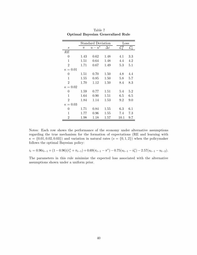
Table 7Optimal Bayesian Generalized Rule

Standard Deviation Losss π u − u∗ ∆i LB

4 L∗

4

RE

0 1.43 0.62 1.48 4.1 3.31 1.51 0.64 1.48 4.4 4.22 1.71 0.67 1.49 5.3 5.1

κ = 0.010 1.51 0.70 1.50 4.8 4.41 1.55 0.85 1.50 5.8 5.72 1.70 1.12 1.50 8.4 8.3

κ = 0.020 1.59 0.77 1.51 5.4 5.21 1.64 0.90 1.51 6.5 6.52 1.84 1.14 1.53 9.2 9.0

κ = 0.030 1.71 0.84 1.55 6.3 6.11 1.77 0.96 1.55 7.4 7.32 1.98 1.18 1.57 10.1 9.7

Notes: Each row shows the performance of the economy under alternative assumptionsregarding the true mechanism for the formation of expectations (RE and learning withκ = {0.01, 0.02, 0.03}) and variation in natural rates (s = {0, 1, 2}) when the policymakerfollows the optimal Bayesian policy:

it = 0.96it−1 + (1− 0.96)(r∗t + πt−1)+ 0.69(πt−1 −π∗)− 0.75(ut−1 − u∗

t )− 2.57(ut−1 −ut−2).

The parameters in this rule minimize the expected loss associated with the alternativeassumptions shown under a uniform prior.

40

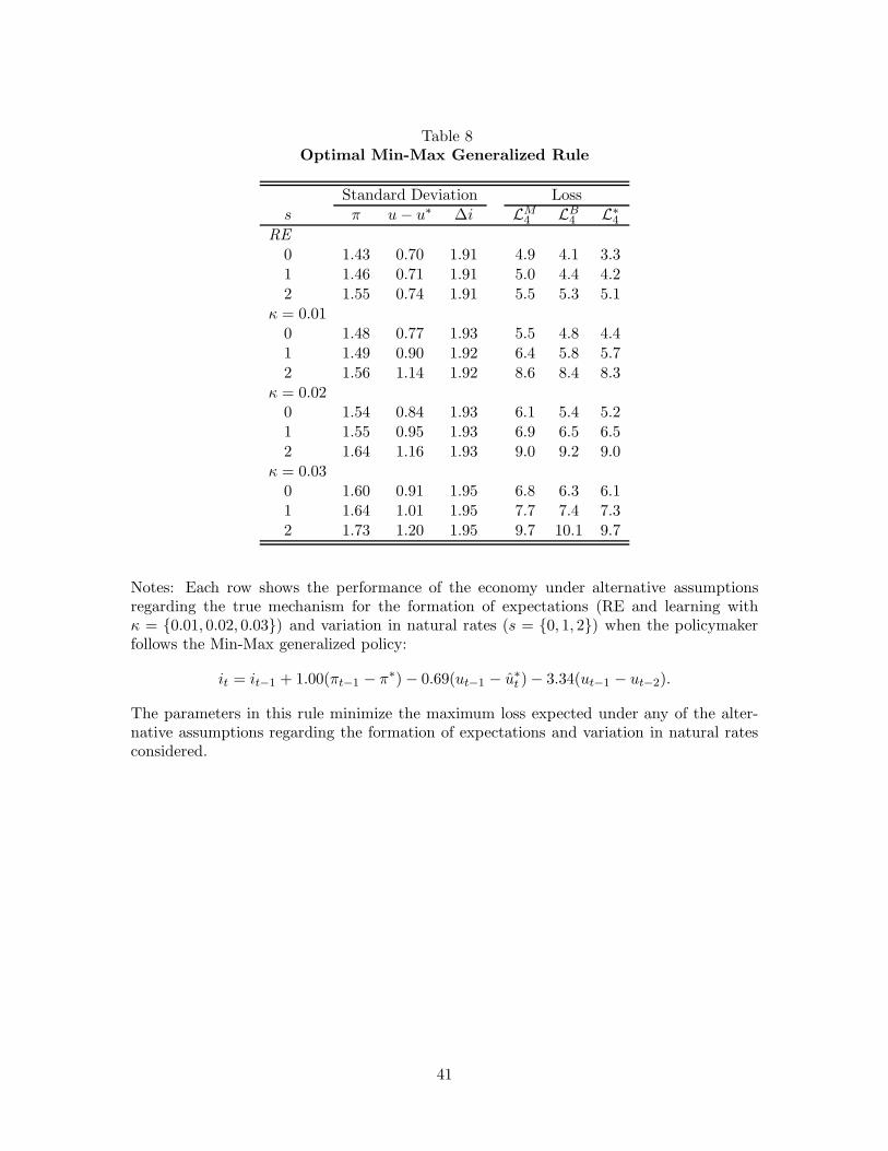
Table 8Optimal Min-Max Generalized Rule

Standard Deviation Losss π u − u∗ ∆i LM

4 LB4 L∗

4

RE

0 1.43 0.70 1.91 4.9 4.1 3.31 1.46 0.71 1.91 5.0 4.4 4.22 1.55 0.74 1.91 5.5 5.3 5.1

κ = 0.010 1.48 0.77 1.93 5.5 4.8 4.41 1.49 0.90 1.92 6.4 5.8 5.72 1.56 1.14 1.92 8.6 8.4 8.3

κ = 0.020 1.54 0.84 1.93 6.1 5.4 5.21 1.55 0.95 1.93 6.9 6.5 6.52 1.64 1.16 1.93 9.0 9.2 9.0

κ = 0.030 1.60 0.91 1.95 6.8 6.3 6.11 1.64 1.01 1.95 7.7 7.4 7.32 1.73 1.20 1.95 9.7 10.1 9.7

Notes: Each row shows the performance of the economy under alternative assumptionsregarding the true mechanism for the formation of expectations (RE and learning withκ = {0.01, 0.02, 0.03}) and variation in natural rates (s = {0, 1, 2}) when the policymakerfollows the Min-Max generalized policy:

it = it−1 + 1.00(πt−1 − π∗) − 0.69(ut−1 − u∗

t ) − 3.34(ut−1 − ut−2).

The parameters in this rule minimize the maximum loss expected under any of the alter-native assumptions regarding the formation of expectations and variation in natural ratesconsidered.

41

Table 9Robust Generalized Rules with Alternative Preferences

Policy Rule Coefficienti π u − u∗ ∆u

λ = 0RE-optimal 0.81 0.32 −0.60 −0.31Bayesian 0.95 0.79 −0.55 −1.06Min-Max 0.99 1.03 −0.46 −1.59

λ = 0.25RE-optimal 0.80 0.30 −0.63 −0.23Bayesian 0.94 0.77 −0.56 −1.16Min-Max 1.00 1.05 −0.55 −1.76

λ = 1.00RE-optimal 0.79 0.26 −0.72 −0.03Bayesian 0.92 0.75 −0.60 −1.58Min-Max 1.00 1.04 −0.57 −2.34

λ = 4.00RE-optimal 0.76 0.18 −0.97 −0.43Bayesian 0.96 0.69 −0.75 −2.57Min-Max 1.00 1.00 −0.69 −3.34

λ = 16.00RE-optimal 0.73 0.11 −1.46 −1.16Bayesian 1.00 0.60 −0.84 −4.02Min-Max 1.00 0.99 −0.97 −5.02

Notes: it = θiit−1 + (1 − θi)(r∗

t + πt−1) + θπ(πt−1 − π∗) + θu(ut−1 − u∗

t ) + θ∆u(ut−1 − ut−2)

42

Table 10Optimal Bayesian and Min-Max Two-Parameter Rules

Min-Max Bayesians LM

T LMD LB

T LBD

RE

0 6.1 5.7 5.3 5.21 6.3 5.8 5.6 5.32 7.0 6.0 6.6 5.7

κ = 0.010 6.8 6.4 6.1 6.01 8.5 7.2 8.0 6.82 11.8 9.3 11.6 9.1

κ = 0.020 7.5 7.1 6.9 6.81 9.1 7.8 8.7 7.62 12.3 9.8 12.4 9.9

κ = 0.030 8.2 7.9 7.6 7.81 9.8 8.6 9.5 8.52 12.9 10.5 13.3 10.7

Notes: Each row compares the loss incurred under alternative assumptions regarding thetrue mechanism for the formation of expectations and variation in natural rates for two-parameter optimal Bayesian and Min-Max policy rules. The corresponding Min-Max rulesfor the level, LM

T , and difference specifications, LMD , are:

it = r∗t + πt−1 + 1.43(πt−1 − π∗) − 0.87(ut−1 − u∗

t )

it = it−1 + 0.95(πt−1 − π∗) − 4.60(ut−1 − ut−2)

The corresponding Bayesian rules for the level, LBT , and difference specifications, LB

D, are:

it = r∗t + πt−1 + 1.07(πt−1 − π∗) − 0.77(ut−1 − u∗

t )

it = it−1 + 0.65(πt−1 − π∗) − 4.12(ut−1 − ut−2).

43

Figure 1

The Taylor Rule Under Learning with Time-Varying Natural Rates

6 6

6

6

88

8

1010

10

12

Rational Expectations

θπ

θu

4.0

0.5 1 1.5 2 2.5 3−6

−5

−4

−3

−2

−1

0

6

6

6

8

8

8

8

8

10

10

10 10

10

1012

12

12 1216

16

16

2020

2030

3050

50

s=1, RE

θπ

θu

5.3

0.5 1 1.5 2 2.5 3−6

−5

−4

−3

−2

−1

0

8

8

8

10

10

10

10

12

12

1212

12

16

16

16

20

20

20

30

30

30

5050

50

s=2, RE

θπ

θu

6.5

0.5 1 1.5 2 2.5 3−6

−5

−4

−3

−2

−1

0

6

6

6

6

8 8

8

8

8

8

8

10

10

10

10

10

1212

12

12

1616

2030

Private Sector Learning: κ = 0.01

θπ

θu

5.4

0.5 1 1.5 2 2.5 3−6

−5

−4

−3

−2

−1

0 8

810

10 10

1012

12

1212

12

1216

16

16

20

20

20

30

3030

5050

s= 1; κ = 0.01

θπ

θu

7.8

0.5 1 1.5 2 2.5 3−6

−5

−4

−3

−2

−1

0

12

12

16

16

16

16

16

20

20

20

30

30

30

5050

50

s= 2; κ = 0.01

θπ

θu

11.4

0.5 1 1.5 2 2.5 3−6

−5

−4

−3

−2

−1

0

8

8

8

8

810

10

10

10

10

10

12

12

12 1212

12

1616

2020

30

Private Sector Learning: κ = 0.02

θπ

θu

6.4

0.5 1 1.5 2 2.5 3−6

−5

−4

−3

−2

−1

0

10

10

10

10

12

1212

12

12

16

16

16

2020

20

3030

30

5050

50

s=1; κ = 0.02

θπ

θu

8.7

0.5 1 1.5 2 2.5 3−6

−5

−4

−3

−2

−1

0

16

16

16

16

16

20

20

2020

30

30

30

5050

50

s= 2; κ = 0.02

θπ

θu

12.2

0.5 1 1.5 2 2.5 3−6

−5

−4

−3

−2

−1

0

8

8

8

8

10

10

10 10

10

10

12

12

12 1212

1216

16

1620

2030

Private Sector Learning: κ = 0.03

θπ

θu

7.3

0.5 1 1.5 2 2.5 3−6

−5

−4

−3

−2

−1

010

10

10

12

12

12

12

1216

16

16

16

20

20

20

20

3030

30

305050

50

50s= 1; κ = 0.03

θπ

θu

9.5

0.5 1 1.5 2 2.5 3−6

−5

−4

−3

−2

−1

016

16

16

16

16

20

20

20

20

30

30

30

50

50

50

s= 2; κ = 0.03

θπ

θu

12.9

0.5 1 1.5 2 2.5 3−6

−5

−4

−3

−2

−1

0

Notes: Each panel shows contours of the loss associated with the Taylor-style policy ruleit = r∗t + πt−1 + θπ(πt−1 − π∗) + θu(ut−1 − u∗

t ) for the assumptions regarding expectationsformation and time-variation of the natural rates shown.

44

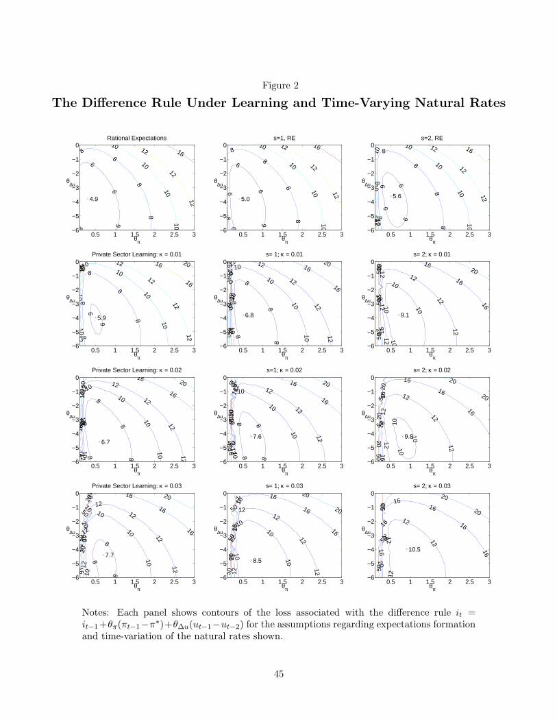
Figure 2

The Difference Rule Under Learning and Time-Varying Natural Rates

6 6

6

6

8

8

88

10

10

10

10

12

12

12

16

Rational Expectations

θπ

θ∆u

4.9

0.5 1 1.5 2 2.5 3−6

−5

−4

−3

−2

−1

0

66

6

6

6

8 8

8

8

810

10

1010

12

12

12

16s=1, RE

θπ

θ∆u

5.0

0.5 1 1.5 2 2.5 3−6

−5

−4

−3

−2

−1

0

6 6

6

68

8

8

8

8

8

1010

10

10

10

1010

12

12

12

12

16

16

s=2, RE

θπ

θ∆u

5.6

0.5 1 1.5 2 2.5 3−6

−5

−4

−3

−2

−1

0

6

6

8

8

8

8

8

1010

1010

10

10

1212

12

12

12

12

16

16

16

2020

Private Sector Learning: κ = 0.01

θπ

θ∆u

5.9

0.5 1 1.5 2 2.5 3−6

−5

−4

−3

−2

−1

0

88

88

8

10

10

10

10

10

10

12

12

12 12

12

12

1216

16

16

16

16

2020

20

20

5050

50

s= 1; κ = 0.01

θπ

θ∆u

6.8

0.5 1 1.5 2 2.5 3−6

−5

−4

−3

−2

−1

0

1010

10

10

1212

12 12

12

1216

16

16

16

16

16

2020

20 20

5050

50

s= 2; κ = 0.01

θπ

θ∆u

9.1

0.5 1 1.5 2 2.5 3−6

−5

−4

−3

−2

−1

0

8

8

8

8

8

1010

10

10

10

1012

1212

12

12

12

12

16

1616

16

162020

2050

50

Private Sector Learning: κ = 0.02

θπ

θ∆u

6.7

0.5 1 1.5 2 2.5 3−6

−5

−4

−3

−2

−1

0

8

8 8

8

1010

10

10

10

1212

12 12

12

12

1616

16

16

16

20

20

20 2050

50

50

50

s=1; κ = 0.02

θπ

θ∆u

7.6

0.5 1 1.5 2 2.5 3−6

−5

−4

−3

−2

−1

0

10

10

10

12

12

12

12

12

16

1616

16

16

16

20

2020

20

20

50

50

50

s= 2; κ = 0.02

θπ

θ∆u

9.8

0.5 1 1.5 2 2.5 3−6

−5

−4

−3

−2

−1

0

8

8

810

10

10

10

10

12

12

12

12

12

1216

16

16

16

16

16

20

20

20

20

50

50

5050Private Sector Learning: κ = 0.03

θπ

θ∆u

7.7

0.5 1 1.5 2 2.5 3−6

−5

−4

−3

−2

−1

0

10

10

10

10

1212

1212

12

12

16

1616

16

16

16

2020

20

20

2050

5050

s= 1; κ = 0.03

θπ

θ∆u

8.5

0.5 1 1.5 2 2.5 3−6

−5

−4

−3

−2

−1

0

12

12

12

12

16

16

1616

16

16

2020

20

20

20

50

50

50

s= 2; κ = 0.03

θπ

θ∆u

10.5

0.5 1 1.5 2 2.5 3−6

−5

−4

−3

−2

−1

0

Notes: Each panel shows contours of the loss associated with the difference rule it =it−1+θπ(πt−1−π∗)+θ∆u(ut−1−ut−2) for the assumptions regarding expectations formationand time-variation of the natural rates shown.

45

Figure 3

The Concern for Robustness: Natural Rate Misperceptions

s

Standard deviation in inflation

0.00 0.25 0.50 0.75 1.00 1.25 1.50 1.75 2.00

1

2

3

4

5

s

Standard deviation in unemployment gap

0.00 0.25 0.50 0.75 1.00 1.25 1.50 1.75 2.00

0.00

0.25

0.50

0.75

1.00

s

Standard deviation in funds rate

0.00 0.25 0.50 0.75 1.00 1.25 1.50 1.75 2.00

0.50

0.75

1.00

1.25

1.50

s

Loss

0.00 0.25 0.50 0.75 1.00 1.25 1.50 1.75 2.00

5

10

15

20Optimized for s = 0Optimized for s = 1Optimized for s = 2

Notes: In each panel, each line plots the asymptotic standard deviation/expected loss thatobtain with a fixed policy rule for a range of natural-rate variation, s, shown in the horizontalaxis. In all simulations expectations are assumed to be rational. The three fixed policiesrepresent the generalized rule optimized for s = {0, 1, 2} under rational expectations.

46

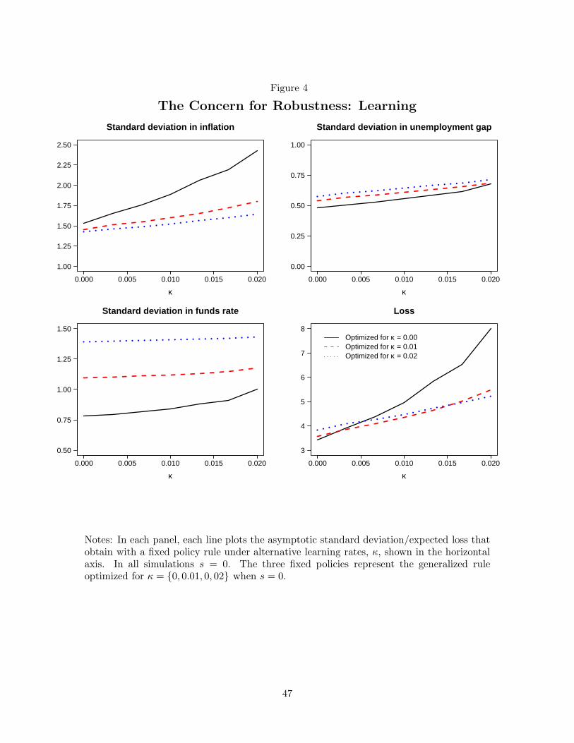
Figure 4

The Concern for Robustness: Learning

κ

Standard deviation in inflation

0.000 0.005 0.010 0.015 0.020

1.00

1.25

1.50

1.75

2.00

2.25

2.50

κ

Standard deviation in unemployment gap

0.000 0.005 0.010 0.015 0.020

0.00

0.25

0.50

0.75

1.00

κ

Standard deviation in funds rate

0.000 0.005 0.010 0.015 0.020

0.50

0.75

1.00

1.25

1.50

κ

Loss

0.000 0.005 0.010 0.015 0.020

3

4

5

6

7

8Optimized for κ = 0.00Optimized for κ = 0.01Optimized for κ = 0.02

Notes: In each panel, each line plots the asymptotic standard deviation/expected loss thatobtain with a fixed policy rule under alternative learning rates, κ, shown in the horizontalaxis. In all simulations s = 0. The three fixed policies represent the generalized ruleoptimized for κ = {0, 0.01, 0, 02} when s = 0.

47