Optimized Jumping of an Articulated Robotic Leg

Junjie Shen1, Yeting Liu1, Xiaoguang Zhang1, and Dennis Hong1

Abstract— This paper proposes a nonlinear programming(NLP) formulation intended for the trajectory optimization oflegged robot jumping applications during the stance phase,taking into consideration the detailed robot model, actuatorcapability, terrain condition, etc. The method is applicable to awide class of jumping robots and was successfully implementedon an articulated robotic leg for jumping in terms of maximumreachable height, minimum energy consumption, as well asoptimum energy efficiency. The simulation and experimentalresults demonstrate that this approach is capable of not onlyplanning one single jumping trajectory, but also designing aperiodic jumping gait for legged robots.

I. INTRODUCTION

Legged robots, despite of increased complexity and powerconsumption compared with other types of mobile robot,have the potential to exert a much larger influence to humanenvironments in the future. The articulated limbs providethem with the inimitable possibility of going anywhere ahuman can go and doing anything a human can do. Whileprogress has been made, legged robots are only beginning tofulfill this great potential.

Traditionally, legged robots are realized with hydraulicactuators for producing tremendous magnitude of force [1],[2]. However, their energy efficiency is limited and theactuation system is often large and difficult to install [3],[4]. Later, legged robots are equipped with electromagnetic(EM) actuators with large gear ratio in order to achievehigh torque density [5]. Nevertheless, these heavily gearedmotors, specifically designed to perform accurate position-controlled tasks in fairly structured environments, are quitevulnerable when faced with significant ground impact forlegged locomotion, due to increased reflected inertia andgear friction from the gearbox [6]. Recently, more advancedlegged robots have been developed which are capable ofdynamic locomotion over irregular terrain with the help ofseries elastic actuators (SEA) [7], [8]. SEAs are utilized tomitigate the ground impact by intentionally adding controlledvariable mechanical impedance in series with an actuator[9]. However, their force bandwidth is limited [10], [11].In addition, these legged systems with added mechanicalimpedance usually result in complex dynamics, making themdifficult to control at best and restricted in their capabilitiesat worst. Lately, impressive advances in EM technology, i.e.,direct-drive [6] and quasi-direct-drive motors [12], [13], [14],

1Junjie Shen, Yeting Liu, Xiaoguang Zhang, and Dennis Hong are withthe Robotics and Mechanisms Laboratory, the Department of Mechani-cal and Aerospace Engineering, University of California, Los Angeles,CA 90095, USA {junjieshen, liu1995, hawkblizzard,dennishong}@ucla.edu

have demonstrated that they are capable of producing suffi-cient torque and speed for legged robot dynamic locomotionwithout high gearing [15], [16]. This leads to the benefit ofhigh transparency and mechanical performance [6], whichenables accurate modeling and control of legged systemswith straightforward torque inputs. In this paper, we willonly focus on legged robots with this type of actuator.

The capability of jumping motions is one of the maincharacters distinguishing legged robots from other types ofmobile robot, which has been extensively studied for severaldecades. Raibert and Brown developed a one-legged hoppingmachine with springy leg of telescopic type and realizeda hopping gait with an empirical controller [2]. Using asimilar controller, Hyon and Mita designed another one-legged hopping robot that had an articulated leg composed ofthree links [17]. A leg spring was further utilized not only toenhance energy efficiency but also to absorb large impulse attouch-down. Arikawa and Mita proposed a practical motionplanning method for jumping motions of multi-degree-of-freedom jumping robot on the basis of the boundary stateat take-off and verified it with simulation of normal jump aswell as somersault [18]. Hutter et al. employed an operationalspace controller to impose the behavior of the spring loadedinverted pendulum (SLIP) model on an articulated roboticleg, which was then capable of continuous hopping onuneven ground [19].

Though many legged systems have been shown to becapable of jumping motions, not until recent the mathe-matical optimization technique is applied to optimize thecontrol strategy for some specific jumping tasks. Lim etal. reduced the jumping trajectory optimization of biartic-ular legged robots to a parameter optimization problem byparameterizing the joint trajectory in terms of B-splines[20]. However, joint torque cannot be constrained directlybut using a penalty function and ground friction was notconsidered. Hiasa et al. used a similar parameterization foreach joint as reference and were able to constrain jointtorque directly with their nonlinear optimization simulationapproach [21]. However, the optimized joint torque wascomputed from a PD controller by following the parame-terized joint reference, which was far from the ideal values.Ding and Park proposed a sequential nonlinear optimizationprocess that simultaneously solved for optimal control inputas well as chose mechanical design parameters specificallyfor single robotic leg jumping task [22]. Nonetheless, the legwas modeled as a simple point mass at the base with groundreaction force (GRF) as input and thus the experimentalresults deviated from the optimized results largely. Withoutconsidering ground friction, slippage happened during the

Fig. 1. Examples of 2D legged robot. On the left is the single leg model; inthe middle is the simplified biped model; and on the right is the simplifiedquadruped model. The world frame is in red.

experiment. Besides, the optimized results were conservativeby enforcing initial GRF to zero. Nguyen et al. presented adifferent nonlinear optimization method for quadruped robotsand successfully implemented it on the MIT Cheetah 3 [23].Nevertheless, the purpose of their cost function is more liketo find a feasible solution than to optimize the jumpingperformance. Besides, only one single jump is considered.

Inspired by the previous work, this paper proposes anonlinear programming (NLP) formulation intended for thetrajectory optimization of legged robot jumping applicationsduring the stance phase, taking into account the detailedrobot model, actuator capability, terrain condition, etc. Themethod was successfully tested on an articulated roboticleg not only for optimizing one single jumping trajectorybut also for designing a periodic jumping gait. The restof this paper is organized as follows. Section II describesthe legged robot model of interest. Section III details thetrajectory optimization algorithm for legged robot jumpingapplications via an NLP formulation. Section IV illustratesthe proposed method with a single degree-of-freedom (DOF)robotic leg for vertical jumping. Section V illustrates theproposed method with a two DOF robotic leg for jumpinggait design. Section VI concludes the paper.

II. ROBOT MODEL

In this paper, we focus on optimizing jumping trajec-tory (during the stance phase right before take-off) for anarticulated robotic leg on the sagittal plane. However, theproposed method can be generalized to a wide class oflegged robots, as shown in Fig. 1. Define the vector ofgeneralized coordinates q =

[x,z,α,θT

]T , where x, z, α arethe body position and angle, and θ is the joint position vectorincluding both actuated joints θa and passive joints θp. Theequations of motion take the form:

M(q)q+C(q, q) =Bτ +J(q)Td, (1)

where M(q) stands for the inertia matrix, the vector C(q, q)captures the Coriolis, centrifugal, and gravitational forces,B defines how the actuation torques τ enter the model, andthe Jocabian matrix J(q) transforms external forces d intogeneralized forces. We can convert (1) into its state-spaceform for the sake of NLP formulation:

x= f(x,τ ,d), (2)

where the state x=[qT , qT

]T and

f(x,τ ,d) =

[q

M(q)−1(Bτ +J(q)Td−C(q, q)

) ] .(3)

Additionally, a kinematics constraint is further imposed tofix each stance foot on the ground before take-off:

h(q) = p, (4)

where p describes the position of stance feet and

∂h(q)

∂q= J(q). (5)

III. PROBLEM FORMULATION

This section illustrates how we formulate the optimizationof jumping trajectory to an NLP for legged robots. First ofall, a typical formulation for a mathematical optimizationproblem can be written as follows:

minimizez

c(z)

subject to φ(z) = 0,

ψ(z)≤ 0,

(6)

where z ∈Rn is the vector of decision variables, c : Rn→Ris the scalar objective function, φ : Rn→ Rm is the equalityconstraint function, and ψ : Rn→ Rr is the inequality con-straint function [24]. At least one of c, φ, and ψ needs tobe nonlinear to make (6) an NLP.

A. Decision Variables

The optimal jumping problem for legged robots is ini-tially a continuous-time trajectory optimization problem.To simplify the integration calculations involved, the directcollocation method is used to discretize the trajectories at Ncollocation points with even time intervals ∆t. We find thattrapezoidal collocation works well here since the durationof stance T is really short for jumping. The set of decisionvariables χ can first be defined as

χ := {q[k], q[k],τ [k],d[k]|k = 1, . . . ,N} , (7)

where q[k], q[k], τ [k], and d[k] are known as the collocationpoints at time t[k] = (k− 1)∆t. To further ensure a smoothand physically feasible profile, polynomials of order S areused to parameterize τ and d, which gives

τ [k] =S

∑i=0λit[k]i, d[k] =

S

∑i=0νit[k]i, k = 1, . . . ,N, (8)

where λi and νi are the vectors of coefficients for themonomial of order i. Parameterization is not further appliedto the states q and q because they are already subject to thedynamics (1), which will end up with a smooth and feasibletrajectory if τ and d are nice functions. The set of decisionvariables χ thus becomes

χ := {q[k], q[k]|k = 1, . . . ,N}∪{Λ,V } , (9)

where Λ = [λ0, . . . ,λS] and V = [ν0, . . . ,νS]. Note that thetotal number of decision variables decreases if S < N−1.

For different applications and interests, χ can also involvedecision variables such as the generalized acceleration q[k],the duration of stance T , the position of stance feet p, themotor gear ratio γ , the link length l, etc.

B. Objective Function

The jumping performance can be evaluated in many differ-ent ways. For example, to maximize the maximum reachableheight hmax of the center of mass (CoM) after take-off, theobjective function c(χ) will be

c(χ) =−hmax =−zCoM[N]− zCoM[N]2

2g, (10)

where g is the gravitational acceleration, zCoM[N] is theheight, and zCoM[N] is the vertical velocity component ofCoM at take-off. Both of them are functions of q[N] andq[N]. In addition, when the leg dynamics is negligiblecompared to the body, (10) can be simplified to

c(χ) =−z[N]− z[N]2

2g, (11)

where z[N] is the height and z[N] is the vertical velocitycomponent of the body at take-off.

Another way to evaluate the jumping performance can beenergy consumption E when the goal height h is fixed. It canbe defined as the integral of the absolute mechanical powerof the actuators over the duration of stance T :

E :=∫ T

0|τ |T

∣∣∣θa

∣∣∣dt, (12)

where θa is the actuated joint velocity vector. The objectivefunction is further approximated as a summation

c(χ) =N−1

∑k=1

12

(|τ [k]|T

∣∣∣θa[k]∣∣∣+ |τ [k+1]|T

∣∣∣θa[k+1]∣∣∣)∆t

= E. (13)

This approximation is done by applying the trapezoid rule forintegration between each adjacent pair of collocation points.We can also combine (10) and (13) together with a tuningweight to take both into consideration.

C. Constraints

1) Dynamics Constraint: It is applied between every ad-jacent pair of collocation points using trapezoidal collocationfollowing [25]:

x[k+1]−x[k] = ∆t2(f [k+1]+f [k]) , k = 1, . . . ,N−1,

(14)

where f [k] = f (x[k],τ [k],d[k]) is the result of evaluatingthe system dynamics at each collocation point. Additionaldecision variable q[k] can be introduced to avoid calculatingthe inverse of the inertia matrix in f .

0c/

max/

Speed

max

Torq

ue

Fig. 2. A typical BLDC motor speed-torque curve scaled by gear ratio γ .

2) Kinematics Constraint: It is applied at each collocationpoint according to (4) and (5):

h(q[k]) = p, k = 1, . . . ,N, (15)

which is the position kinematics constraint and

h(q[k]) = J(q[k])q[k] = 0, k = 1, . . . ,N, (16)

which is the velocity kinematics constraint. If q[k] is alsoinvolved as decision variable, a third acceleration kinematicsconstraint needs to be imposed as well by taking further timederivative of (16).

3) Motor Constraint: A typical brushless DC electricmotor (BLDC motor) speed-torque curve scaled by gearratio γ is shown in Fig. 2. Considering the combination ofboth positive and negative values, the constraint on actuatedjoint velocity and actuation torque can be formulated as thefollowing polyhedron at each collocation point:

I 0−I 0I γbI−I γbII −γbI−I −γbI

[τ [k]θa[k]

]≤

γτmax1γτmax1bωmax1bωmax1bωmax1bωmax1

, k = 1, . . . ,N,

(17)

where I is the identity matrix, 1 = [1, . . . ,1]T is of the samelength as τ [k] or θa[k], and b = γτmax/(ωc−ωmax).

4) Friction Cone Constraint: It is applied for each stancefoot at each collocation point to prevent slippage:∣∣∣d( j)

x [k]∣∣∣≤ µ

∣∣∣d( j)z [k]

∣∣∣ , j = 1, . . . ,M, k = 1, . . . ,N, (18)

where d( j)[k] =[d( j)

x [k],d( j)z [k]

]Tis the GRF acting on the

jth stance foot at the kth collocation point and µ is thecoefficient of friction between the stance foot and ground.Since a stance foot cannot pull the ground, i.e., d( j)

z [k] ≥ 0for all j and k, (18) is reduced to 0 −1

1 −µ

−1 −µ

[ d( j)x [k]

d( j)z [k]

]≤ 0, j = 1, . . . ,M,

k = 1, . . . ,N. (19)

If the ground is inclined, (19) can be further modified to 0 −11 −µ

−1 −µ

[ cosβ sinβ

−sinβ cosβ

][d( j)

x [k]d( j)

z [k]

]≤ 0,

j = 1, . . . ,M, k = 1, . . . ,N, (20)

where β is the inclination angle.5) Take-off Constraint: Some special constraints need to

be taken into consideration, which makes it different fromother types of trajectory optimization for legged robots. Tomake sure the robot will jump (leave the ground) afterwards,the last collocation point is considered as the moment of take-off. That is, the GRF should be zero for each stance foot andthe CoM velocity component normal to the ground shouldbe positive at the last collocation point:

d( j)[N] = 0, j = 1, . . . ,M, (21)−xCoM[N]sinβ + zCoM[N]cosβ ≥ 0. (22)

6) Other Constraints: Some other constraints can beincluded on a case-by-case basis, such as the initial andfinal configuration constraint, joint angle range constraint,external force constraint, etc. In general, these constraintscan be formulated in a linear manner.

D. Complete Formulation

The complete NLP formulation of the jumping trajectoryoptimization problem for legged robots is thus given by

minimizeχ

c(χ)

subject to Dynamics Constraint (14),Kinematics Constraint (15)(16),Motor Constraint (17),Friction Cone Constraint (20),Take-off Constraint (21)(22),Other Constraints,

(23)

where the nonlinearity usually comes from the robot model,i.e., (14), (15), and (16).

IV. EXAMPLE OF A SINGLE DOF ROBOTIC LEG

This section explores the optimal jumping problem for asingle DOF robotic leg via the NLP formulation.

A. Single DOF Robotic Leg Model

Fig. 3 shows the single DOF robotic leg model in detail.The body with mass M is mounted on a vertical linearguide with horizontal position x = xo. Its vertical positionis denoted as z. The femur and tibia links share the samemass m, length l, and inertia J. The point foot is mountedon another vertical linear guide with horizontal position p.Therefore, the friction cone constraint is not considered here.The only BLDC motor with gear ratio γ is mounted on thebody and the femur joint θ1 is actuated while the tibia jointθ2 is passive. The equations of motion take the form as (1),where q = [x,z,θ1,θ2]

T , Bτ = [0,0,τ,0]T , d = [dx,dz,dr]T .

[dx,dz]T is the GRF acted on the foot and dr is the external

Fig. 3. Single DOF robotic leg model. The world frame is in red. The twolinear giudes are shown by the dashed gray lines.

force exerted on the body by the linear guide in the xdirection. An extra constant friction term d f from the linearguide in the z directional is also considered in the model.The kinematics constraint (4) gives

h(q) =

x+ l cosθ1 + l cos(θ1 +θ2)z− l sinθ1− l sin(θ1 +θ2)

x

=

p0xo

, (24)

and the Jacobian matrix can be computed from (5) as

J(q) =

1 0 −l (sinθ1 + sin(θ1 +θ2)) −l sin(θ1 +θ2)0 1 −l (cosθ1 + cos(θ1 +θ2)) −l cos(θ1 +θ2)1 0 0 0

.(25)

The robot parameters are listed in TABLE I.

TABLE IROBOT PARAMETERS

Symbol Parameter Value & UnitM Body mass 0.88 kgm Link mass 0.085 kgl Link length 0.2 mJ Link inertia 4.3×10−4 kg·m2

τmax Maximum torque 0.42 N·mωc Cutoff speed 1755 rad/s

ωmax Maximum speed 1910 rad/sγ Gear ratio 24

B. Maximum Reachable Height

To maximize the maximum reachable height hmax, theNLP is formulated as follows

minimizeχ

Objective Function (11)

subject to Dynamics Constraint (14),Kinematics Constraint (15)(16),Motor Constraint (17),Take-off Constraint (21)(22),Other Constraints,

(26)

where the set of decision variables χ is defined as

χ := {q[k], q[k]|k = 1, . . . ,N}∪{Λ,V , p,T} . (27)

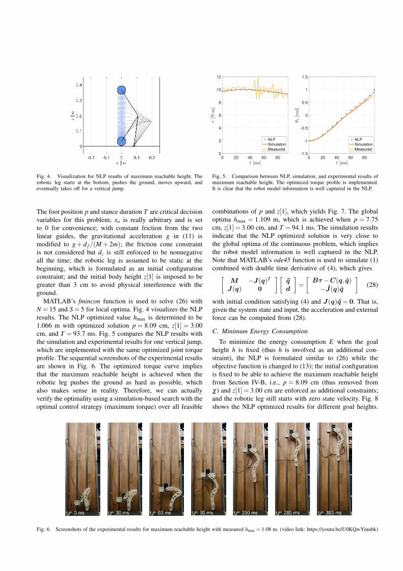
Fig. 4. Visualization for NLP results of maximum reachable height. Therobotic leg starts at the bottom, pushes the ground, moves upward, andeventually takes off for a vertical jump.

The foot position p and stance duration T are critical decisionvariables for this problem; xo is really arbitrary and is setto 0 for convenience; with constant friction from the twolinear guides, the gravitational acceleration g in (11) ismodified to g+ d f /(M + 2m); the friction cone constraintis not considered but dz is still enforced to be nonnegativeall the time; the robotic leg is assumed to be static at thebeginning, which is formulated as an initial configurationconstraint; and the initial body height z[1] is imposed to begreater than 3 cm to avoid physical interference with theground.

MATLAB’s fmincon function is used to solve (26) withN = 15 and S = 5 for local optima. Fig. 4 visualizes the NLPresults. The NLP optimized value hmax is determined to be1.066 m with optimized solution p = 8.09 cm, z[1] = 3.00cm, and T = 93.7 ms. Fig. 5 compares the NLP results withthe simulation and experimental results for one vertical jump,which are implemented with the same optimized joint torqueprofile. The sequential screenshots of the experimental resultsare shown in Fig. 6. The optimized torque curve impliesthat the maximum reachable height is achieved when therobotic leg pushes the ground as hard as possible, whichalso makes sense in reality. Therefore, we can actuallyverify the optimality using a simulation-based search with theoptimal control strategy (maximum torque) over all feasible

0 20 40 60 800

2

4

6

8

10

12

NLP

Simulation

Measured

0 20 40 60 80-1.5

-1

-0.5

0

0.5

1

1.5

NLP

Simulation

Measured

Fig. 5. Comparison between NLP, simulation, and experimental results ofmaximum reachable height. The optimized torque profile is implemented.It is clear that the robot model information is well captured in the NLP.

combinations of p and z[1], which yields Fig. 7. The globaloptima hmax = 1.109 m, which is achieved when p = 7.75cm, z[1] = 3.00 cm, and T = 94.1 ms. The simulation resultsindicate that the NLP optimized solution is very close tothe global optima of the continuous problem, which impliesthe robot model information is well captured in the NLP.Note that MATLAB’s ode45 function is used to simulate (1)combined with double time derivative of (4), which gives[

M −J(q)T

J(q) 0

][qd

]=

[Bτ −C(q, q)

−J(q)q

](28)

with initial condition satisfying (4) and J(q)q = 0. That is,given the system state and input, the acceleration and externalforce can be computed from (28).

C. Minimum Energy Consumption

To minimize the energy consumption E when the goalheight h is fixed (thus h is involved as an additional con-straint), the NLP is formulated similar to (26) while theobjective function is changed to (13); the initial configurationis fixed to be able to achieve the maximum reachable heightfrom Section IV-B, i.e., p = 8.09 cm (thus removed fromχ) and z[1] = 3.00 cm are enforced as additional constraints;and the robotic leg still starts with zero state velocity. Fig. 8shows the NLP optimized results for different goal heights.

Fig. 6. Screenshots of the experimental results for maximum reachable height with measured hmax = 1.08 m. (video link: https://youtu.be/U0KQwYinubk)

0.6

15

0.7

0.8

0.9

10

1

10

1.1

55

3 0

0.65

0.7

0.75

0.8

0.85

0.9

0.95

1

1.05

1.1

Fig. 7. Simulation results of maximum reachable height under differentcombinations of foot position p and initial body height z[1]. The globaloptima hmax = 1.109 m with p = 7.75 cm and z[1] = 3.00 cm.

The blue line shows the optimized minimum energy con-sumption at each goal height. It is a monotonically increasingfunction over the given feasible domain, which makes physi-cal sense. Furthermore, the idea of the dimensionless specificmechanical cost of transport [26] is used as a measure of theenergy efficiency of the system over one vertical jump, whichis defined as

η =E

(M+2m)g(h− z[1]), (29)

where h− z[1] is the overall vertical distance traveled. Thered line in Fig. 8 tells that η is minimized when h is around0.6 m, i.e., the most energy-efficient way of vertical jumpingis when the goal height is set to 0.6 m. We will later apply theidea of η when designing optimum jumping gait for leggedrobots in terms of energy efficiency.

V. EXAMPLE OF A TWO DOF ROBOTIC LEG

This section investigates the optimum jumping gait for atwo DOF robotic leg via the NLP formulation. A conceptdiagram is shown in Fig. 9.

A. Two DOF Robotic Leg Model

The two DOF robotic leg model is almost the same asthe single one in Section IV-A but without the two linearguides. In addition, both the femur and tibia joints are nowactuated. The equations of motion take the form as (1),where q = [x,z,θ1,θ2]

T , Bτ = [0,0,τ1,τ2]T , d = [dx,dz]

T .The kinematics constraint (4) gives

h(q) =

[x+ l cosθ1 + l cos(θ1 +θ2)z− l sinθ1− l sin(θ1 +θ2)

]=

[p0

], (30)

where the foot position p is now actually arbitrary and isthus set to 0 for convenience. The Jacobian matrix can becomputed from (5) as

J(q) =

[1 0 −l (sinθ1 + sin(θ1 +θ2)) −l sin(θ1 +θ2)0 1 −l (cosθ1 + cos(θ1 +θ2)) −l cos(θ1 +θ2)

].

(31)

0.4 0.5 0.6 0.7 0.8 0.9 1.0 1.0665

10

15

20

1.5

1.55

1.6

1.65

1.7

1.75

1.8Minimum Energy Consumption

Minimum Cost of Transport

Fig. 8. NLP results of minimum energy consumption for different goalheights. The red line indicates the vertical jumping is most energy-efficientwhen the goal height h is around 0.6 m.

B. Optimum Jumping Gait

We aim to design an optimum periodic jumping gait forthe two DOF robotic leg in terms of energy efficiency viathe NLP formulation. The set of decision variables χ is firstdefined as

χ := {q[k], q[k]|k = 1, . . . ,N}∪{Λ,V ,T} . (32)

In spite of the constraints illustrated in Section III-C, someother constraints need to be imposed to ensure periodicity ofthe jumping gait. For simplicity, after take-off, the body ofthe robotic leg is assumed to be a projectile without consid-ering the leg dynamics during the flight phase. Therefore, therelationship between the final configuration and the config-uration just before touch-down (q− =

[x−,z−,θ−1 ,θ−2

]T andq− =

[x−, z−, θ−1 , θ−2

]T ) is given by

x[N] = x− = vd , (33)(z−)2− z[N]2 = 2g

(z[N]− z−

). (34)

(33) indicates a constant desired horizontal velocity vd < 0throughout the flight phase while (34) determines the changein vertical velocity component based on the height change.By assuming an impulsive and perfectly plastic collision, thetouch-down impact model is formulated according to [27] as

M(q[1])(q[1]− q−

)= J(q[1])Tξ, (35)

Fig. 9. One complete cycle of the 2 DOF robotic leg jumping gait. Itstarts from the right after the touch-down impact, pushes the ground, takesoff, travels in the air, eventually lands, and completes the cycle. The worldframe is in red. The amber line describes the body trajectory.

where the additional decision variable ξ is the impact forcefrom the ground to the foot, the initial generalized velocityq[1] represents the velocity right after the impact and theinitial position q[1] is assumed to be invariant through theimpact, i.e., q[1] = q−. The two links are also assumed tobe able to already return to their initial configuration by theend of the flight phase, i.e., θ

−1 = θ

−2 = 0.

To optimize the jumping gait in terms of energy efficiency,the idea of cost of transport η is applied yet with modifica-tions to (29), since the problem is now in two dimensions.The total horizontal distance traveled ∆x for one jump can besimply measured by the change in foothold on the ground,which is given by

∆x = x[1]+ x f − x[N], (36)

where x[1]≥ 0, x[N]≤ 0 from Fig. 9, and

x f =−vd ·z[N]− z−

g, (37)

which is computed based on the projectile assumption of thebody during the flight phase. Therefore, η can be defined as

η =E

(M+2m)g∆x. (38)

The jumping height is not further considered because x falready captures that information, i.e., given vd , ∆x willincrease if the height increases and vice versa. The NLPis finally formulated as follows

minimizeχ , ξ

Objective Function (38)

subject to Dynamics Constraint (14),Kinematics Constraint (15)(16),Motor Constraint (17),Friction Cone Constraint (19),Take-off Constraint (21)(22),Gait Constraint (33)(34)(35),Other Constraints.

(39)

Fig. 10. Visualization for NLP results of optimum jumping gait. Therobotic leg starts from the right after the touch-down impact, pushes theground, travels to the left, and eventually takes off for the next jump.

MATLAB’s fmincon function is used to solve (39) withvd = −1 m/s, µ = 1, β = 0, N = 15, and S = 5, yieldingthe optimized jumping gait with η = 1.26, as shown in Fig.10. The robotic leg starts from the right-hand side right afterthe touch-down impact, pushes the ground, travels to the left,and eventually takes off for the next jump. MATLAB’s ode45function is used to verify the NLP results and the simulationresults are shown in Fig. 11. During the flight phase, a simple

Fig. 11. Simulation results of optimum jumping gait. Figure (a) visualizesthe critical moments in the simulation, e.g., touch-down, take-off, midpointduring the flight phase. The amber, green, and brown lines describe thetrajectories of the robot body, CoM, and foot, respectively. Starting at theorigin, the robotic leg is able to complete four planned jumps to the leftbefore divergence. The rest figures compares the simulation results with theNLP results for the first two jumps. The shaded area represents the stancephase while the white area represents the flight phase. Figure (b) shows thebody velocity. The desired horizontal velocity vd =−1 m/s. The simulationresults validate the projectile assumption of the body during the flight phase.Figure (c) shows the two joint angles. They are forced to follow a predefinedtrajectory during the flight phase via a PD controller. Figure (d) shows theactuation torques. The same torque profile is implemented in the simulationas suggested by the NLP results. Figure (e) shows the ground reaction force.The NLP results ensure that no slippage happens with µ = 1.

joint level PD controller is implemented to drive the two linksto its desired configuration for the upcoming stance phase.With only open-loop control during the stance phase, therobotic leg is able to complete more or less four plannedjumps before divergence, which indicates the proposed NLPformulation is good enough for designing periodic jumpinggait for legged robots.

VI. CONCLUSION

In this paper, a trajectory optimization algorithm specifi-cally served for legged robot jumping applications during thestance phase was presented in detail via a nonlinear program-ming (NLP) formulation, in consideration of robot full-bodydynamics and kinematics, actuator capability, terrain condi-tion, etc. The method is applicable to a wide class of jumpingrobots and was successfully implemented on an articulatedrobotic leg as an example. Optimized jumping trajectorieswere investigated in terms of maximum reachable height,minimum energy consumption, as well as optimum energyefficiency. The simulation and experimental demonstrationsverify that this approach is capable of not only optimizingone single jumping trajectory, but also designing a periodicjumping gait for legged robots. In spite of initial guess andlocal optima issues, the detailed robot model information,i.e., dynamics and kinematics where the nonlinearity usuallycomes from, is well captured in the NLP. For that reason, theNLP results can be almost directly tested in the simulationand experimental environments with desired outcomes. Ourfuture plan is to study optimum landing strategy for leggedrobots after take-off.

ACKNOWLEDGMENT

This work is partially supported by ONR through grantN00014-15-1-2064. The authors thank the Robotics andMechanisms Laboratory (RoMeLa) at UCLA.

REFERENCES

[1] M. H. Raibert, Legged Robots That Balance. MIT Press, 1986.[2] M. H. Raibert and H. B. Brown, Jr., “Experiments in Balance With

a 2D One-Legged Hopping Machine,” Journal of Dynamic Systems,Measurement, and Control, vol. 106, pp. 75–81, 03 1984.

[3] M. Raibert, K. Blankespoor, G. Nelson, and R. Playter, “Bigdog, therough-terrain quadruped robot,” IFAC Proceedings Volumes, vol. 41,no. 2, pp. 10822 – 10825, 2008. 17th IFAC World Congress.

[4] S. Kuindersma, R. Deits, M. Fallon, A. Valenzuela, H. Dai, F. Per-menter, T. Koolen, P. Marion, and R. Tedrake, “Optimization-basedlocomotion planning, estimation, and control design for the atlashumanoid robot,” Autonomous Robots, vol. 40, pp. 429–455, Mar2016.

[5] K. Hirai, M. Hirose, Y. Haikawa, and T. Takenaka, “The developmentof honda humanoid robot,” in Proceedings. 1998 IEEE InternationalConference on Robotics and Automation (Cat. No.98CH36146), vol. 2,pp. 1321–1326 vol.2, May 1998.

[6] G. Kenneally, A. De, and D. E. Koditschek, “Design principles for afamily of direct-drive legged robots,” IEEE Robotics and AutomationLetters, vol. 1, pp. 900–907, July 2016.

[7] A. Ramezani, J. W. Hurst, K. Akbari Hamed, and J. W. Grizzle,“Performance Analysis and Feedback Control of ATRIAS, A Three-Dimensional Bipedal Robot,” Journal of Dynamic Systems, Measure-ment, and Control, vol. 136, 12 2013. 021012.

[8] M. Hutter, C. Gehring, D. Jud, A. Lauber, C. D. Bellicoso, V. Tsounis,J. Hwangbo, K. Bodie, P. Fankhauser, M. Bloesch, R. Diethelm,S. Bachmann, A. Melzer, and M. Hoepflinger, “Anymal - a highly mo-bile and dynamic quadrupedal robot,” in 2016 IEEE/RSJ InternationalConference on Intelligent Robots and Systems (IROS), pp. 38–44, Oct2016.

[9] M. Hutter, C. Gehring, M. A. Hopflinger, M. Blosch, and R. Siegwart,“Toward combining speed, efficiency, versatility, and robustness inan autonomous quadruped,” IEEE Transactions on Robotics, vol. 30,pp. 1427–1440, Dec 2014.

[10] G. A. Pratt and M. M. Williamson, “Series elastic actuators,” inProceedings 1995 IEEE/RSJ International Conference on IntelligentRobots and Systems. Human Robot Interaction and CooperativeRobots, vol. 1, pp. 399–406 vol.1, Aug 1995.

[11] D. W. Robinson, J. E. Pratt, D. J. Paluska, and G. A. Pratt, “Serieselastic actuator development for a biomimetic walking robot,” in1999 IEEE/ASME International Conference on Advanced IntelligentMechatronics (Cat. No.99TH8399), pp. 561–568, Sep. 1999.

[12] P. M. Wensing, A. Wang, S. Seok, D. Otten, J. Lang, and S. Kim,“Proprioceptive actuator design in the mit cheetah: Impact mitigationand high-bandwidth physical interaction for dynamic legged robots,”IEEE Transactions on Robotics, vol. 33, pp. 509–522, June 2017.

[13] S. Kalouche, “Design for 3d agility and virtual compliance usingproprioceptive force control in dynamic legged robots,” Master’sthesis, Carnegie Mellon University, Pittsburgh, PA, August 2016.

[14] T. Zhu, J. Hooks, and D. Hong, “Design, modeling, and analysisof a liquid cooled proprioceptive actuator for legged robots,” in2019 IEEE/ASME International Conference on Advanced IntelligentMechatronics (AIM), pp. 36–43, July 2019.

[15] G. Bledt, M. J. Powell, B. Katz, J. Di Carlo, P. M. Wensing, andS. Kim, “Mit cheetah 3: Design and control of a robust, dynamicquadruped robot,” in 2018 IEEE/RSJ International Conference onIntelligent Robots and Systems (IROS), pp. 2245–2252, Oct 2018.

[16] J. Yu, J. Hooks, X. Zhang, M. Sung Ahn, and D. Hong, “A pro-prioceptive, force-controlled, non-anthropomorphic biped for dynamiclocomotion,” in 2018 IEEE-RAS 18th International Conference onHumanoid Robots (Humanoids), pp. 1–9, Nov 2018.

[17] S. H. Hyon and T. Mita, “Development of a biologically inspiredhopping robot-”kenken”,” in Proceedings 2002 IEEE InternationalConference on Robotics and Automation (Cat. No.02CH37292), vol. 4,pp. 3984–3991 vol.4, May 2002.

[18] K. Arikawa and T. Mita, “Design of multi-dof jumping robot,” inProceedings 2002 IEEE International Conference on Robotics andAutomation (Cat. No.02CH37292), vol. 4, pp. 3992–3997 vol.4, May2002.

[19] M. Hutter, C. D. Remy, M. A. Hopflinger, and R. Siegwart, “Slip run-ning with an articulated robotic leg,” in 2010 IEEE/RSJ InternationalConference on Intelligent Robots and Systems, pp. 4934–4939, Oct2010.

[20] B. Lim, J. Babic, and F. C. Park, “Optimal jumps for biarticularlegged robots,” in 2008 IEEE International Conference on Roboticsand Automation, pp. 226–231, May 2008.

[21] S. Hiasa, R. Sato, A. Ming, F. Meng, H. Liu, X. Fan, X. Chen,Z. Yu, and Q. Huang, “Development of a bipedal robot with bi-articular muscle-tendon complex between hip and knee joint,” in 2018IEEE International Conference on Cyborg and Bionic Systems (CBS),pp. 391–396, Oct 2018.

[22] Y. Ding and H. Park, “Design and experimental implementation ofa quasi-direct-drive leg for optimized jumping,” in 2017 IEEE/RSJInternational Conference on Intelligent Robots and Systems (IROS),pp. 300–305, Sep. 2017.

[23] Q. Nguyen, M. J. Powell, B. Katz, J. D. Carlo, and S. Kim, “Optimizedjumping on the mit cheetah 3 robot,” in 2019 International Conferenceon Robotics and Automation (ICRA), pp. 7448–7454, May 2019.

[24] S. Boyd and L. Vandenberghe, Convex Optimization. New York, NY,USA: Cambridge University Press, 2004.

[25] M. Kelly, “An introduction to trajectory optimization: How to do yourown direct collocation,” SIAM Review, vol. 59, no. 4, pp. 849–904,2017.

[26] S. Collins, A. Ruina, R. Tedrake, and M. Wisse, “Efficient bipedalrobots based on passive-dynamic walkers,” Science, vol. 307, no. 5712,pp. 1082–1085, 2005.

[27] Y. Hurmuzlu and D. B. Marghitu, “Rigid body collisions of planarkinematic chains with multiple contact points,” The InternationalJournal of Robotics Research, vol. 13, no. 1, pp. 82–92, 1994.