optimal power flow (dc-opf and ac-opf)
TRANSCRIPT
Optimal Power Flow (DC-OPF and AC-OPF)
DTU Summer School 2018
Spyros Chatzivasileiadis

What is optimal power flow?
2 DTU Electrical Engineering Optimal Power Flow (DC-OPF and AC-OPF) Jun 25, 2018
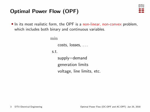
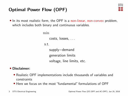
Optimal Power Flow (OPF)
• In its most realistic form, the OPF is a non-linear, non-convex problem,which includes both binary and continuous variables.
min
costs, losses, . . .
s.t.
supply=demand
generation limits
voltage, line limits, etc.
• Disclaimer:
• Realistic OPF implementations include thousands of variables andconstraints• Here we focus on the most “fundamental” formulations of OPF
3 DTU Electrical Engineering Optimal Power Flow (DC-OPF and AC-OPF) Jun 25, 2018
Outline
• Economic Dispatch
• DC-OPF
• AC-OPF
4 DTU Electrical Engineering Optimal Power Flow (DC-OPF and AC-OPF) Jun 25, 2018
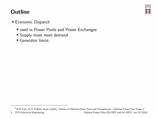
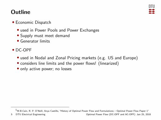
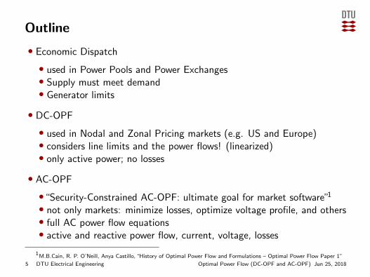
Outline
• Economic Dispatch
• used in Power Pools and Power Exchanges• Supply must meet demand• Generator limits
• DC-OPF
• used in Nodal and Zonal Pricing markets (e.g. US and Europe)• considers line limits and the power flows! (linearized)• only active power; no losses
• AC-OPF
•“Security-Constrained AC-OPF: ultimate goal for market software”1
• not only markets: minimize losses, optimize voltage profile, and others• full AC power flow equations• active and reactive power flow, current, voltage, losses
1M.B.Cain, R. P. O’Neill, Anya Castillo, “History of Optimal Power Flow and Formulations – Optimal Power Flow Paper 1”
5 DTU Electrical Engineering Optimal Power Flow (DC-OPF and AC-OPF) Jun 25, 2018
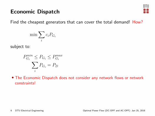
Economic Dispatch
Find the cheapest generators that can cover the total demand! How?
min∑i
ciPGi
subject to:
PminGi≤ PGi
≤ PmaxGi∑
i
PGi= PD
• The Economic Dispatch does not consider any network flows or networkconstraints!
•We assume a copperplate network, i.e. a lossless and unrestricted flow ofelectricity from A to B.
6 DTU Electrical Engineering Optimal Power Flow (DC-OPF and AC-OPF) Jun 25, 2018
Can we solve the economic dispatch problem without using anoptimization solver?
Yes! With the help of the merit order curve.
7 DTU Electrical Engineering Optimal Power Flow (DC-OPF and AC-OPF) Jun 25, 2018

Can we solve the economic dispatch problem without using anoptimization solver?
Yes! With the help of the merit order curve.
7 DTU Electrical Engineering Optimal Power Flow (DC-OPF and AC-OPF) Jun 25, 2018

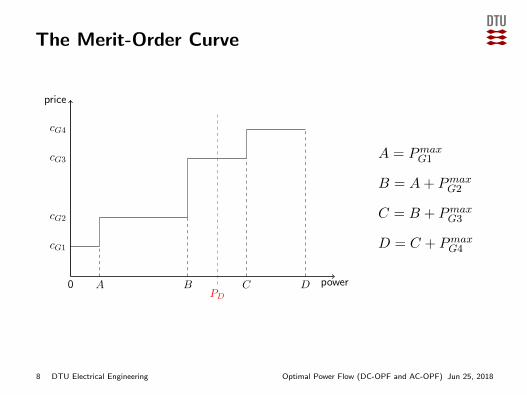
The Merit-Order Curve
0 A B C D
cG1
cG2
cG3
cG4
price
power
PD
A = PmaxG1
B = A+ PmaxG2
C = B + PmaxG3
D = C + PmaxG4
8 DTU Electrical Engineering Optimal Power Flow (DC-OPF and AC-OPF) Jun 25, 2018
The Merit-Order Curve
0 A B C D
cG1
cG2
cG3
cG4
price
powerPD
A = PmaxG1
B = A+ PmaxG2
C = B + PmaxG3
D = C + PmaxG4
8 DTU Electrical Engineering Optimal Power Flow (DC-OPF and AC-OPF) Jun 25, 2018

The Merit-Order Curve
0 A B C D
cG1
cG2
cG3
cG4
price
powerPD
• cG3 is the systemmarginal price
• G1 and G2 fullydispatched
• G4 not dispatched
• G3 partially dispatched:“marginal generator”
9 DTU Electrical Engineering Optimal Power Flow (DC-OPF and AC-OPF) Jun 25, 2018
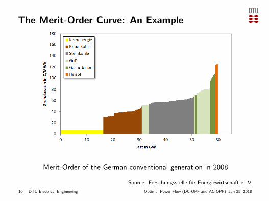
The Merit-Order Curve: An Example
Merit-Order of the German conventional generation in 2008
Source: Forschungsstelle fur Energiewirtschaft e. V.
10 DTU Electrical Engineering Optimal Power Flow (DC-OPF and AC-OPF) Jun 25, 2018
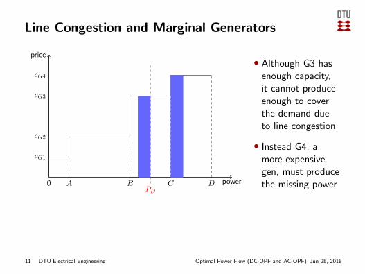
Line Congestion and Marginal Generators
0 A B C D
cG1
cG2
cG3
cG4
price
powerPD
• Although G3 hasenough capacity,it cannot produceenough to coverthe demand dueto line congestion
• Instead G4, amore expensivegen, must producethe missing power
• In a DC-OPF context, there is no longer a single system marginal price(we will observe different nodal prices in different nodes)
11 DTU Electrical Engineering Optimal Power Flow (DC-OPF and AC-OPF) Jun 25, 2018
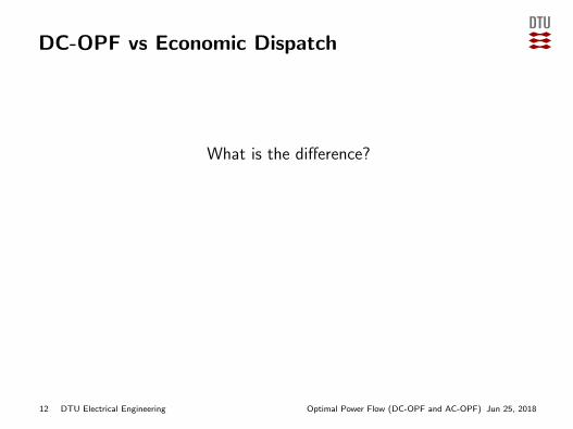
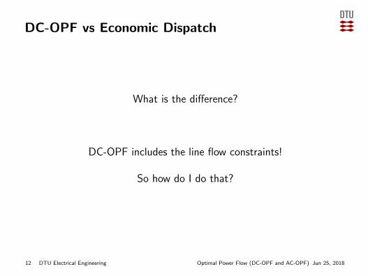
DC-OPF vs Economic Dispatch
What is the difference?
DC-OPF includes the line flow constraints!
So how do I do that?
12 DTU Electrical Engineering Optimal Power Flow (DC-OPF and AC-OPF) Jun 25, 2018
DC-OPF vs Economic Dispatch
What is the difference?
DC-OPF includes the line flow constraints!
So how do I do that?
12 DTU Electrical Engineering Optimal Power Flow (DC-OPF and AC-OPF) Jun 25, 2018

DC-OPF vs Economic Dispatch
What is the difference?
DC-OPF includes the line flow constraints!
So how do I do that?
12 DTU Electrical Engineering Optimal Power Flow (DC-OPF and AC-OPF) Jun 25, 2018
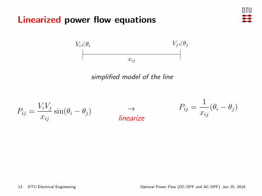
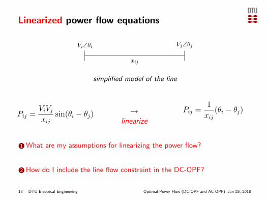
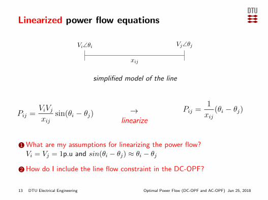
Linearized power flow equations
Vi∠θi Vj∠θj
xij
simplified model of the line
Pij =ViVjxij
sin(θi − θj) →linearize
Pij =1
xij(θi − θj)
1 What are my assumptions for linearizing the power flow?
Vi = Vj = 1p.u and sin(θi − θj) ≈ θi − θj
2 How do I include the line flow constraint in the DC-OPF?
13 DTU Electrical Engineering Optimal Power Flow (DC-OPF and AC-OPF) Jun 25, 2018
Linearized power flow equations
Vi∠θi Vj∠θj
xij
simplified model of the line
Pij =ViVjxij
sin(θi − θj) →linearize
Pij =1
xij(θi − θj)
1 What are my assumptions for linearizing the power flow?Vi = Vj = 1p.u and sin(θi − θj) ≈ θi − θj
2 How do I include the line flow constraint in the DC-OPF?
13 DTU Electrical Engineering Optimal Power Flow (DC-OPF and AC-OPF) Jun 25, 2018
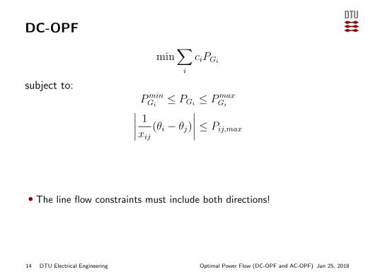
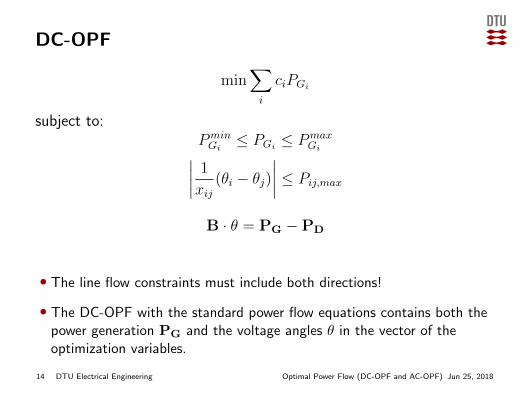
DC-OPF
min∑i
ciPGi
subject to:PminGi≤ PGi
≤ PmaxGi∣∣∣∣ 1xij (θi − θj)
∣∣∣∣ ≤ Pij,max
B · θ = PG −PD
• The line flow constraints must include both directions!
• The DC-OPF with the standard power flow equations contains both thepower generation PG and the voltage angles θ in the vector of theoptimization variables.
14 DTU Electrical Engineering Optimal Power Flow (DC-OPF and AC-OPF) Jun 25, 2018

Exercise
1 2
3
cG1 = 60 $/MWh, cG2 = 120 $/MWh
Pload = 150 MW
PmaxG1 = 100 MW, Pmax
G2 = 200 MW
X12 = 0.1 pu, X13 = 0.3 pu, X23 = 0.1 pu,BaseMVA = 100 MVA
Pmax13 = 40 MW (line limit)
1 What are the optimization variables? Form theoptimization vector
2 Formulate the objective function
3 Formulate the constraints
15 DTU Electrical Engineering Optimal Power Flow (DC-OPF and AC-OPF) Jun 25, 2018

DC-OPF in Matlab
How would you transfer yourproblem formulation to Matlab?
How do you calculate the nodalprices?
16 DTU Electrical Engineering Optimal Power Flow (DC-OPF and AC-OPF) Jun 25, 2018
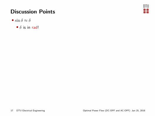
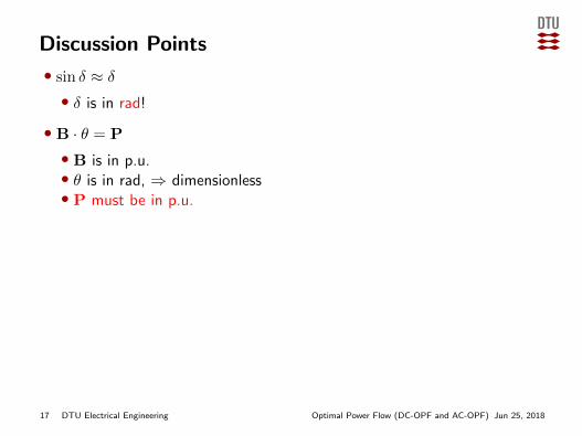
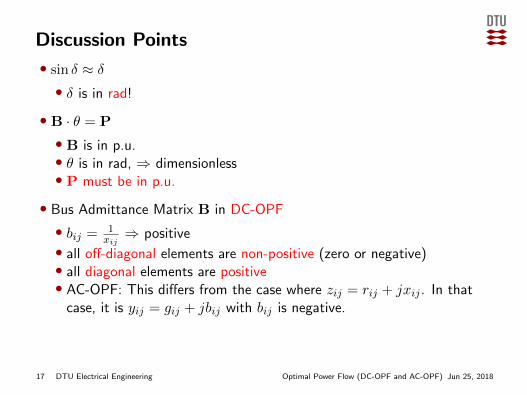
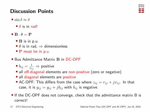
Discussion Points
• sin δ ≈ δ• δ is in rad!
• B · θ = P
• B is in p.u.• θ is in rad, ⇒ dimensionless• P must be in p.u.
• Bus Admittance Matrix B in DC-OPF
• bij = 1xij⇒ positive
• all off-diagonal elements are non-positive (zero or negative)• all diagonal elements are positive• AC-OPF: This differs from the case where zij = rij + jxij . In that
case, it is yij = gij + jbij with bij is negative.
• If the DC-OPF does not converge, check that the admittance matrix B iscorrect!
17 DTU Electrical Engineering Optimal Power Flow (DC-OPF and AC-OPF) Jun 25, 2018
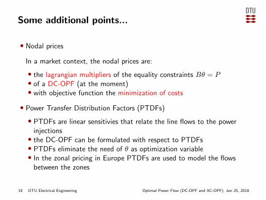
Some additional points...
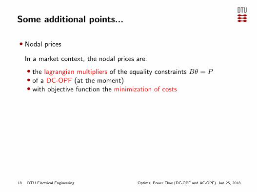
• Nodal prices
In a market context, the nodal prices are:
• the lagrangian multipliers of the equality constraints Bθ = P• of a DC-OPF (at the moment)• with objective function the minimization of costs
• Power Transfer Distribution Factors (PTDFs)
• PTDFs are linear sensitivies that relate the line flows to the powerinjections• the DC-OPF can be formulated with respect to PTDFs• PTDFs eliminate the need of θ as optimization variable• In the zonal pricing in Europe PTDFs are used to model the flows
between the zones
18 DTU Electrical Engineering Optimal Power Flow (DC-OPF and AC-OPF) Jun 25, 2018
Some additional points...
• Nodal prices
In a market context, the nodal prices are:
• the lagrangian multipliers of the equality constraints Bθ = P• of a DC-OPF (at the moment)• with objective function the minimization of costs
• Power Transfer Distribution Factors (PTDFs)
• PTDFs are linear sensitivies that relate the line flows to the powerinjections• the DC-OPF can be formulated with respect to PTDFs• PTDFs eliminate the need of θ as optimization variable• In the zonal pricing in Europe PTDFs are used to model the flows
between the zones
18 DTU Electrical Engineering Optimal Power Flow (DC-OPF and AC-OPF) Jun 25, 2018
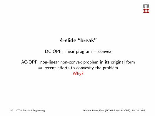
4-slide “break”
DC-OPF: linear program = convex
AC-OPF: non-linear non-convex problem in its original form⇒ recent efforts to convexify the problem
Why?
19 DTU Electrical Engineering Optimal Power Flow (DC-OPF and AC-OPF) Jun 25, 2018

Convex vs. Non-convex Problem
Convex Problem Non-convex problem
x
Cost f(x)
x
Costf(x)
One global minimum Several local minima
20 DTU Electrical Engineering Optimal Power Flow (DC-OPF and AC-OPF) Jun 25, 2018
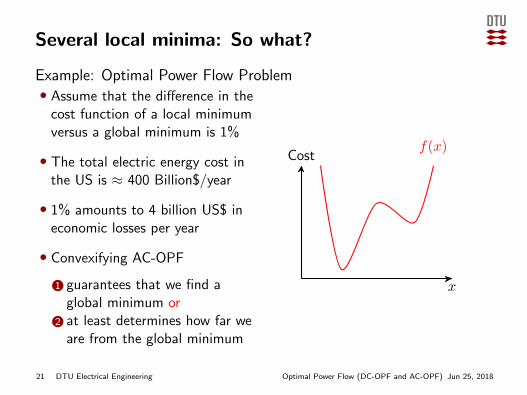
Several local minima: So what?
Example: Optimal Power Flow Problem• Assume that the difference in the
cost function of a local minimumversus a global minimum is 1%
• The total electric energy cost inthe US is ≈ 400 Billion$/year
• 1% amounts to 4 billion US$ ineconomic losses per year
• Convexifying AC-OPF
1 guarantees that we find aglobal minimum or
2 at least determines how far weare from the global minimum
x
Costf(x)
21 DTU Electrical Engineering Optimal Power Flow (DC-OPF and AC-OPF) Jun 25, 2018

Convexifying the Optimal Power Flow problem(OPF)
• Convex relaxations transform theOPF to a convex Semi-DefiniteProgram (SDP)
• Under certain conditions, theobtained solution is the globaloptimum to the original OPFproblem2
x
Costf(x)
Convex Relaxation
2Javad Lavaei and Steven H Low. “Zero duality gap in optimal power flow problem”. In: IEEETransactions on Power Systems 27.1 (2012), pp. 92–10722 DTU Electrical Engineering Optimal Power Flow (DC-OPF and AC-OPF) Jun 25, 2018

Convexifying the Optimal Power Flow problem(OPF)
• Convex relaxations transform theOPF to a convex Semi-DefiniteProgram (SDP)
• Under certain conditions, theobtained solution is the globaloptimum to the original OPFproblem2
x
Costf(x)f(x)
Convex Relaxation
2Javad Lavaei and Steven H Low. “Zero duality gap in optimal power flow problem”. In: IEEETransactions on Power Systems 27.1 (2012), pp. 92–10722 DTU Electrical Engineering Optimal Power Flow (DC-OPF and AC-OPF) Jun 25, 2018

Convexifying the Optimal Power Flow problem(OPF)
• Convex relaxations transform theOPF to a convex Semi-DefiniteProgram (SDP)
• Under certain conditions, theobtained solution is the globaloptimum to the original OPFproblem2 x
Costf(x)f(x)
Convex Relaxation
2Javad Lavaei and Steven H Low. “Zero duality gap in optimal power flow problem”. In: IEEETransactions on Power Systems 27.1 (2012), pp. 92–10722 DTU Electrical Engineering Optimal Power Flow (DC-OPF and AC-OPF) Jun 25, 2018
Break is over...More in 1 hour and in Pascal’s talk tomorrow!
Be patient :)
23 DTU Electrical Engineering Optimal Power Flow (DC-OPF and AC-OPF) Jun 25, 2018
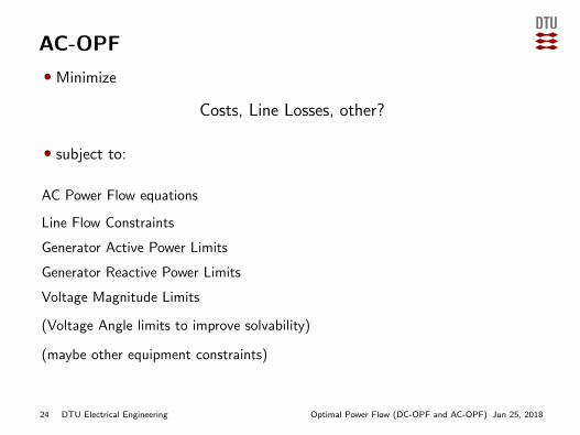
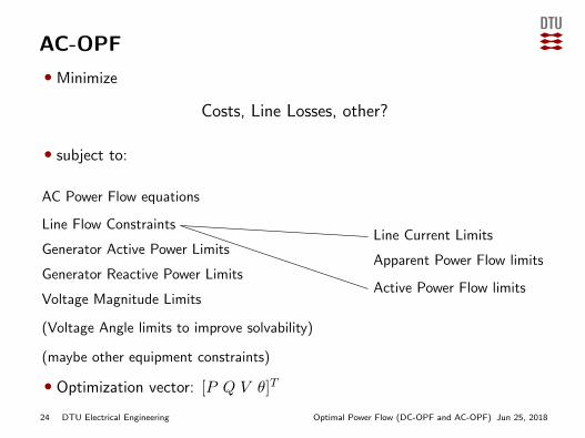
AC-OPF
• Minimize
Costs, Line Losses, other?
• subject to:
AC Power Flow equations
Line Flow Constraints
Generator Active Power Limits
Generator Reactive Power Limits
Voltage Magnitude Limits
(Voltage Angle limits to improve solvability)
(maybe other equipment constraints)
Line Current Limits
Apparent Power Flow limits
Active Power Flow limits
• Optimization vector: [P Q V θ]T
24 DTU Electrical Engineering Optimal Power Flow (DC-OPF and AC-OPF) Jun 25, 2018
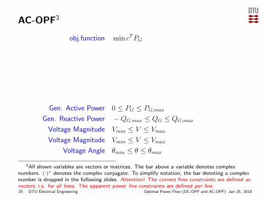
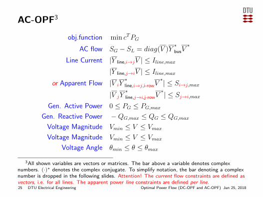
AC-OPF3
obj.function min cTPG
AC flow SG − SL = diag(V )Y∗busV
∗
Line Current |Y line,i→jV | ≤ Iline,max
|Y line,j→iV | ≤ Iline,max
or Apparent Flow |V iY∗line,i→j,i-rowV
∗| ≤ Si→j,max
|V jY∗line,j→i,j-rowV
∗| ≤ Sj→i,max
Gen. Active Power 0 ≤ PG ≤ PG,max
Gen. Reactive Power −QG,max ≤ QG ≤ QG,max
Voltage Magnitude Vmin ≤ V ≤ Vmax
Voltage Magnitude Vmin ≤ V ≤ Vmax
Voltage Angle θmin ≤ θ ≤ θmax
3All shown variables are vectors or matrices. The bar above a variable denotes complexnumbers. (·)∗ denotes the complex conjugate. To simplify notation, the bar denoting a complexnumber is dropped in the following slides. Attention! The current flow constraints are defined asvectors, i.e. for all lines. The apparent power line constraints are defined per line.25 DTU Electrical Engineering Optimal Power Flow (DC-OPF and AC-OPF) Jun 25, 2018

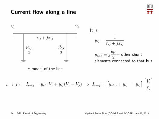
Current flow along a line
Vi Vj
rij + jxij
jbij2
jbij2
π-model of the line
It is:
yij =1
rij + jxij
ysh,i = jbij2+ other shunt
elements connected to that bus
i→ j : Ii→j = ysh,iVi + yij(Vi − Vj) ⇒ Ii→j =[ysh,i + yij −yij
] [ViVj
]
j → i : Ij→i = ysh,jVj + yij(Vj − Vi) ⇒ Ij→i =[−yij ysh,j + yij
] [ViVj
]
26 DTU Electrical Engineering Optimal Power Flow (DC-OPF and AC-OPF) Jun 25, 2018

Current flow along a line
Vi Vj
rij + jxij
jbij2
jbij2
π-model of the line
It is:
yij =1
rij + jxij
ysh,i = jbij2+ other shunt
elements connected to that bus
i→ j : Ii→j = ysh,iVi + yij(Vi − Vj) ⇒ Ii→j =[ysh,i + yij −yij
] [ViVj
]
j → i : Ij→i = ysh,jVj + yij(Vj − Vi) ⇒ Ij→i =[−yij ysh,j + yij
] [ViVj
]26 DTU Electrical Engineering Optimal Power Flow (DC-OPF and AC-OPF) Jun 25, 2018

Line Admittance Matrix Yline
• Yline is an L×N matrix, where L is the number of lines and N is thenumber of nodes
• if row k corresponds to line i− j:
• Yline,ki = ysh,i + yij• Yline,kj = −yij
• yij =1
rij + jxijis the admittance of line ij
• ysh,i is the shunt capacitance jbij/2 of the π-model of the line
•We must create two Yline matrices. One for i→ j and one for j → i
27 DTU Electrical Engineering Optimal Power Flow (DC-OPF and AC-OPF) Jun 25, 2018
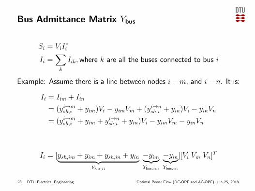
Bus Admittance Matrix Ybus
Si = ViI∗i
Ii =∑k
Iik,where k are all the buses connected to bus i
Example: Assume there is a line between nodes i−m, and i− n. It is:
Ii = Iim + Iin
= (yi→msh,i + yim)Vi − yimVm + (yi→n
sh,i + yin)Vi − yinVn= (yi→m
sh,i + yim + yi→nsh,i + yin)Vi − yimVm − yinVn
Ii = [ysh,im + yim + ysh,in + yin︸ ︷︷ ︸Ybus,ii
−yim︸ ︷︷ ︸Ybus,im
−yin︸︷︷︸Ybus,in
][Vi Vm Vn]T
28 DTU Electrical Engineering Optimal Power Flow (DC-OPF and AC-OPF) Jun 25, 2018
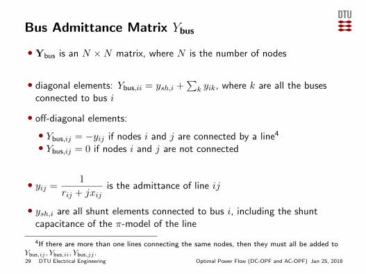
Bus Admittance Matrix Ybus
• Ybus is an N ×N matrix, where N is the number of nodes
• diagonal elements: Ybus,ii = ysh,i +∑
k yik, where k are all the busesconnected to bus i
• off-diagonal elements:
• Ybus,ij = −yij if nodes i and j are connected by a line4
• Ybus,ij = 0 if nodes i and j are not connected
• yij =1
rij + jxijis the admittance of line ij
• ysh,i are all shunt elements connected to bus i, including the shuntcapacitance of the π-model of the line
4If there are more than one lines connecting the same nodes, then they must all be added toYbus,ij , Ybus,ii, Ybus,jj .29 DTU Electrical Engineering Optimal Power Flow (DC-OPF and AC-OPF) Jun 25, 2018
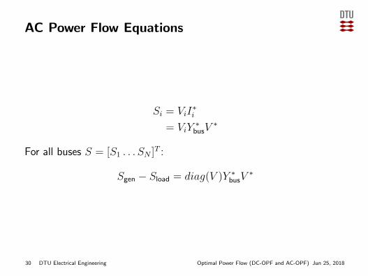
AC Power Flow Equations
Si = ViI∗i
= ViY∗
busV∗
For all buses S = [S1 . . . SN ]T :
Sgen − Sload = diag(V )Y ∗busV∗
30 DTU Electrical Engineering Optimal Power Flow (DC-OPF and AC-OPF) Jun 25, 2018

Further reading
• Resources about AC-OPF from the US Federal Energy RegulatoryCommission (FERC)
https://www.ferc.gov/industries/electric/indus-act/
market-planning/opf-papers.asp
• Overview paper on Economic Dispatch and DC-OPF:
R.D. Christie, B. F. Wollenberg, I. Wangesteen, Transmission Management in the DeregulatedEnvironment, Proceedings of the IEEE, vol. 88, no. 2, February 2000
• DTU Lecture slides: Optimization in modern power systems
http://www.chatziva.com/teaching/2017/31765.html
• Line Congestion, Nodal Prices, and Marginal Generators
S. Chatzivasileiadis, T. Krause, and G. Andersson. HVDC line placement for maximizing socialwelfare - an analytical approach. In IEEE Powertech 2013, pages 1 -6, June 2013.
31 DTU Electrical Engineering Optimal Power Flow (DC-OPF and AC-OPF) Jun 25, 2018
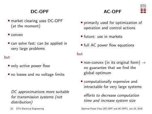
DC-OPF AC-OPF
• market clearing uses DC-OPF(at the moment)
• convex
• can solve fast; can be applied invery large problems
but
• only active power flow
• no losses and no voltage limits
DC approximations more suitablefor transmission systems (notdistribution)
• primarily used for optimization ofoperation and control actions
• future: use in markets
• full AC power flow equations
but
• non-convex (in its original form) →no guarantee that we find theglobal optimum
• computationally expensive andintractable for very large systems
efforts to decrease computationtime and increase system size
32 DTU Electrical Engineering Optimal Power Flow (DC-OPF and AC-OPF) Jun 25, 2018

Thank you!
33 DTU Electrical Engineering Optimal Power Flow (DC-OPF and AC-OPF) Jun 25, 2018
Appendix
34 DTU Electrical Engineering Optimal Power Flow (DC-OPF and AC-OPF) Jun 25, 2018
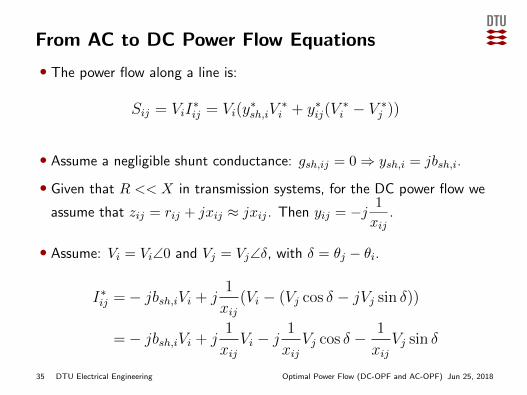
From AC to DC Power Flow Equations
• The power flow along a line is:
Sij = ViI∗ij = Vi(y
∗sh,iV
∗i + y∗ij(V
∗i − V ∗j ))
• Assume a negligible shunt conductance: gsh,ij = 0⇒ ysh,i = jbsh,i.
• Given that R << X in transmission systems, for the DC power flow we
assume that zij = rij + jxij ≈ jxij . Then yij = −j1
xij.
• Assume: Vi = Vi∠0 and Vj = Vj∠δ, with δ = θj − θi.
I∗ij =− jbsh,iVi + j1
xij(Vi − (Vj cos δ − jVj sin δ))
=− jbsh,iVi + j1
xijVi − j
1
xijVj cos δ −
1
xijVj sin δ
35 DTU Electrical Engineering Optimal Power Flow (DC-OPF and AC-OPF) Jun 25, 2018

From AC to DC Power Flow Equations (cont.)
• Since Vi is a real number, it is:
Pij =<{Sij} = Vi<{I∗ij} = −1
xijViVj sin δ
•With δ = θj − θi, it is:
Pij =1
xijViVj sin(θi − θj)
•We further make the assumptions that:
• Vi, Vj are constant and equal to 1 p.u.• sin θ ≈ θ, θ must be in rad
Then
Pij =1
xij(θi − θj)
36 DTU Electrical Engineering Optimal Power Flow (DC-OPF and AC-OPF) Jun 25, 2018