OPTIMAL MULTI-FLOOR PROCESS PLANT

LAYOUT WITH PRODUCTION SECTIONS

Jude O. Ejeha, Songsong Liub, Lazaros G. Papageorgioua,∗

aCentre for Process Systems Engineering, Department of Chemical Engineering, University

College London, London WC1E 7JE, UKbSchool of Management, Swansea University, Bay Campus, Fabian Way, Swansea SA1

8EN, UK

Abstract

This paper addresses the multi-�oor process plant layout problem by developingfour mixed integer linear programming (MILP) models. The problem involvesdecisions concerning the optimal spatial arrangement of process plant equip-ment and/or auxiliary units considering equipment connectivity, pumping andconstruction costs, and other factors. These considerations are extended toaccount for tall equipment that spans across �oors and the availability of pre-de�ned production sections. The proposed models determine simultaneouslythe number of �oors per section, �oor areas, plot layout and site layout, andare applied to two case studies with up to 22 units and 6 production sections todemonstrate their applicability.

Keywords: multi-�oor process plant layout, mixed integer linearprogramming (MILP), production sections, optimisation

1. Introduction

The design of a chemical process plant involves the application of scienti�ctheories and principles, with engineering judgement, to develop an idea from theconceptual stage until completion [22]. This process typically involves feasibilitystudies of the economics and market, design data development, detailed engin-eering designs and economics, procurement and construction, with step by stepresult testing [22]. The detailed engineering designs comprise the estimation ofprocess operating conditions, equipment speci�cations, costs and overall layout;with the last consideration of particular concern to this work.Chemical process plant layout design seeks to determine how best equipmentand associated structures required can be placed within a given physical loc-ation, considering their interconnections, the general safety and operability ofthe plant, as well as the ease and e�ciency of construction and operation [14].

∗Corresponding author. Tel: +44 (0)20 7679 2563Email address: l.papageorgiou@ucl.ac.uk (Lazaros G. Papageorgiou)

Preprint submitted to Elsevier 6th August 2018

In practice, layout considerations can be separated into three as outline byMoran[14] in a "brown�eld": site layout - relating to how plots are placed rel-ative to each other in a site; plot layout - layout of process units within a plot;and equipment layout - arranging process units auxiliaries about the individualunit [14]. The �nal layout can then be determined through a combination ofintuition, economic optimisation, critical examination, equipment ratings, math-ematical modelling, and/or 3D CAD software; the �rst method being regardedas informal and less deterministic.A more precise and informed approach is by mathematical modelling, were mod-els are solved by proven algorithms to determine an optimal layout based onprede�ned conditions. This method has gained popularity in the past three dec-ades amongst researchers and quite a number of models have been developedover time. The primary focus has been given to the realisation of a minimalcost [4]. This cost relates to equipment interconnections by pipes, horizontal andvertical pumping [4, 17], installation of safety equipment [21], in a single �oorand multi-�oor scenario [19]; considering equipment representations in 2D and3D with irregular shapes [1]. The mathematical models, most times, have beenformulated as mixed integer non-linear programming (MINLP) [21] or mixedinteger linear programming (MILP) models [1, 20], being able to handle a fewprocess units in modest computational times. Improved algorithms [20, 24] havealso been developed to successfully handle more process units, but recent workshave employed other solution techniques [3, 8, 15, 16, 18, 23].Multi-�oor layout considerations in process plants have become important in re-cent times owing to growing concerns of space availability, exorbitant land costs,the need to save land for future extensions [6] or where the available layout areaalready has multiple �oors, e.g., in o�shore platforms [10]. Also, the existence oftall equipment that spans across �oors (which is quite prevalent in most chem-ical processes) inadvertently presents a multi-�oor scenario. These have led toa number of factors being considered in the literature as it relates to multi-�oorlayout: routing and layout of pipes [5], safety and risk assessment [13, 23], tallequipment [7, 10, 23], area minimisation [9], to name a few. However, consid-eration of production sections/segregations has not been given much attention,though its widespread practice. With production sections/segregations, di�er-ent parts of the entire chemical process plant are grouped and placed adjacentto each other [12] in what can be referred to as a plot layout [14]. Such group-ings aid in safety and loss prevention, housekeeping, and e�cient constructionand maintenance of equipment [12]. Papageorgiou and Rotstein [17] proposed amathematical modelling approach for single-�oor process plant layout with pro-duction sections. Equipment was pre-allocated sections and the optimal layoutwithin each section and amongst sections was simultaneously determined. Res-ults showed an increase in total cost due to sectioning, but the formulation couldonly handle a limited number of units in a single �oor case. This work seeksto present mathematical models to handle larger scale multi-�oor process plantlayouts in production sections, with tall equipment that spans across �oors.The considerations in this work constitute an extension of the work by Ejehet al. [2], where MILP models were proposed to obtain the optimal multi-�oor

2

layout of a plant considering tall equipment spanning multiple �oors with con-nections at design-speci�ed heights amongst equipment. Model solutions gavethe optimal number of �oors, equipment �oor location and position consideringconnection, construction and pumping costs. Four models (broadly divided intoformulations A and B based on the modelling of tall equipment) were proposed.In formulation A, tall equipment was modelled as a single continuous unit span-ning through �oors by three alternative sets of equations. In formulation B, tallequipment was split into single-�oor pseudo units occupying contiguous �oors.Each of these models was tested with case studies of up to 17 units and optimalsolutions were obtained in reasonable computational times. In this work, pro-duction sections are introduced and the optimal number of �oors and area persection are determined.In the remaining part of this paper, section 2 gives a description of the problemto be solved; the mathematical formulation is described in section 3; and casestudies are presented in section 4 to show the model performance and features.Finally, concluding remarks of the major �ndings are highlighted in section 5.

2. Problem Description

This works aims to obtain the optimal multi-�oor process plant layout withpre-de�ned production sections. The production section is the key feature ofthe problem in this work and refers to a well-de�ned rectangular area spanningacross �oors containing a pre-de�ned subset of equipment items. This featurepromotes plant safety, operability, maintenance activity and workforce manage-ment.Throughout this paper the following assumptions are made:

• The geometries of all process plant equipment and production sections areapproximated as rectangles.

• Distances between equipment and/or sections are rectilinear from theirgeometrical centres in the x-y plane. Vertical distances are taken from adesign-speci�ed height on the equipment unique to each case study.

• Each equipment must belong to only one section, and such section is pre-de�ned.

• Each of the available sections starts from the ground �oor upwards, havingan optimal number of �oors less than or equal to the total number ofavailable �oors.

• The position coordinates of production sections are calculated with respectto the origin of the base land area, and the equipment position coordinateswith respect to the origin of the production section to which they belong.

• Both equipment and production sections can be rotated 90◦ in the x-yplane as deemed optimal, but must start from the base of the �oor it hasbeen assigned.

3

• Any equipment with a height greater than the �oor height is allowed toextend through contiguous �oors.

The problem description is given as follows.Given:

• a set of process units and their dimensions (length, depth and height);

• a set of sections with equipment allocation;

• a set of potential �oors;

• connectivity network amongst process units;

• cost data (connection, pumping, land, and construction);

• �oor height;

• space and unit allocation limitations;

• minimum safety distances between process units;

to determine:

• total number of required �oors for each section for the layout;

• base land area occupied;

• area of �oors;

• area of each section and the �oors in which they are located;

• site and plot layout;

so as to: minimise the total plant layout cost associated with connection, pump-ing, land purchase and �oor construction across production sections.

3. Mathematical Formulation

Nomenclature

Indices

i,j equipment item in models A.1 - A.3i′,j′ equipment item in model Bk �oor numbers rectangular area sizest, u sections/production modules

4

Sets

I set of equipment item for models A.1 - A.3I ′ set of equipment item for model B; I ′ = (I \MF ) ∪

⋃i∈MF

Pi

It set of equipment item i in section tI ′t set of equipment item i′ in section tMF set of multi-�oor equipmentPi sets of pseudo units for multi-�oor equipment iP 1 set of pseudo units of each multi-�oor equipment item i assigned

to the lowest �oor

Parameters

BM , BM ′ large numbersCcij connection costs between items i and jChij horizontal pumping costs between items i and jCvij vertical pumping costs between items i and jDeminij minimum safety distance between items i and jDsmintu minimum safety distance between sections t and ufij 1 if �ow direction between equipment items i and j is

positive; 0, otherwiseFC1 �xed �oor construction costFC2 area-dependent �oor construction costLC land costMi number of �oors required by equipment item iXs, Y s x-y dimensions of pre-de�ned rectangular area sizes s

Integer variables

NFmax maximum number of �oors required across all sectionsNF ′t number of �oors required by section t

Binary variables

Nij 1 if items i and j are assigned to the same �oor; 0, otherwiseQ′st 1 if rectangular area s is selected for section t in the layout;

0, otherwiseS1tu, S2tu non-overlapping binary, a set of values which prevents

production section overlap in one direction in the x-y planeSsik 1 if item i begins on �oor k; 0, otherwiseVik 1 if item i is assigned to �oor kW ′kt 1 if �oor k in section t is occupied; 0, otherwise

5

Continuous variables

Aij relative distance in y coordinates between items i and j,if i is above j

AR′st prede�ned rectangular �oor area s for section tBij relative distance in y coordinates between items i and j,

if i is below jdi breadth of item idtt breadth of production section tFA base land areaFA′t area of section tFA2′kt area of �oor k in section tli length of item iLij relative distance in x coordinates between items i and j,

if i is to the left of jltt length of production section tNQ′st linearisation variable expressing the product of NF ′t and Q

′st

Rij relative distance in x coordinates between items i and j,if i is to the right of j

TDij total rectilinear distance between items i and jxi, yi relative coordinates of the geometrical centre of item ixtt, ytt absolute coordinates of the geometrical centre of production

section t on base land areaXmax, Y max dimensions of base land area

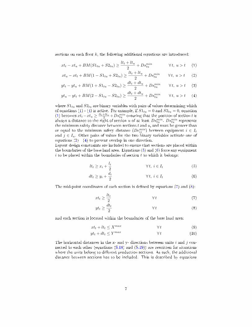
The mathematical formulation constitutes an extension to the formulationsproposed by Ejeh et al. [2] as summarized in Appendix A. These formulationsare broadly classi�ed into "A" and "B". In formulation A, tall equipment ismodelled as a single continuous unit spanning across contiguous �oors, andthree equivalent sets of equations (models A.1, A.2 and A.3) are proposed todescribe this. In formulation B, tall equipment is split into single �oor pseudo-units equivalent to the number of �oors such equipment will span through. Thepseudo-units are then assigned to the same positions on consecutive �oors, andthe model determines the optimal starting �oors. All of these considerations,however, ignore production section restrictions. These four models (Models A.1,A.2, A.3 and B) are thus modi�ed, with new constraints introduced. Theseconstraints prevent overlapping amongst sections and allow for placement ofequipment in the appropriate section. It also builds on the model proposed byPapageorgiou and Rotstein[17] to account for production sections but furtherdetermines the optimal number and size of �oors per section:

3.1. Formulation A

Formulation A consists of three alternative sets of equations for the tallequipment. For each of these equations, in order to prevent overlap of production

6

sections on each �oor k, the following additional equations are introduced:

xtt − xtu +BM(S1tu + S2tu) ≥ltt + ltu

2+Dsmintu ∀ t, u > t (1)

xtu − xtt +BM(1− S1tu + S2tu) ≥ltt + ltu

2+Dsmintu ∀ t, u > t (2)

ytt − ytu +BM(1 + S1tu − S2tu) ≥dtt + dtu

2+Dsmintu ∀ t, u > t (3)

ytu − ytt +BM(2− S1tu − S2tu) ≥dtt + dtu

2+Dsmintu ∀ t, u > t (4)

where S1tu and S2tu are binary variables with pairs of values determining whichof equations (1) - (4) is active. For example, if S1tu = 0 and S2tu = 0, equation(1) becomes xtt−xtu ≥ ltt+ltu

2 +Dsmintu ensuring that the position of section t isalways a distance to the right of section u of at least Dsmintu . Dsmintu representsthe minimum safety distance between sections t and u, and must be greater thanor equal to the minimum safety distance (Deminij ) between equipment i ∈ Itand j ∈ Iu. Other pairs of values for the two binary variables activate one ofequations (2) - (4) to prevent overlap in one direction.Layout design constraints are included to ensure that sections are placed withinthe boundaries of the base land area. Equations (5) and (6) force any equipmenti to be placed within the boundaries of section t to which it belongs:

ltt ≥ xi +li2

∀ t, i ∈ It (5)

dtt ≥ yi +di2

∀ t, i ∈ It (6)

The mid-point coordinates of each section is de�ned by equations (7) and (8):

xtt ≥ltt2

∀ t (7)

ytt ≥dtt2

∀ t (8)

and each section is located within the boundaries of the base land area:

xtt + ltt ≤ Xmax ∀ t (9)

ytt + dtt ≤ Y max ∀ t (10)

The horizontal distances in the x- and y- directions between units i and j con-nected to each other (equations (S.18) and (S.19)) are rewritten for situationswhere the units belong to di�erent production sections. As such, the additionaldistance between sections has to be included. This is described by equations

7

(11) and (12):

Rij − Lij = (xtt −ltt2

+ xi)− (xtu −ltu2

+ xj)

∀ i, j : fij = 1; u ≥ t; i ∈ It; j ∈ Iu(11)

Aij −Bij = (ytt −dtt2

+ yi)− (ytu −dtu2

+ yj)

∀ i, j : fij = 1; u ≥ t; i ∈ It; j ∈ Iu(12)

For cases where units i and j belong to the same section (u = t), equations (11)and (12) reduce to equations (S.18) and (S.19).Equipment �oor constraints from Ejeh et al. [2] (equations (S.2) - (S.6)) aremodi�ed to equations (13) - (17) as follows:

Nij ≥ Vik + Vjk − 1 ∀ i, j > i, k (13)

The variable Nij is de�ned by equation (13), with a value of 1 if equipmentitems i and j are assigned a same �oor, and 0 otherwise.In order to prevent the top �oors in some sections from being empty, it isnecessary to determine the total number of �oors required by each section, asopposed to having a maximum number across sections:

Ssik ≤W ′kt ∀ t, i ∈ It \MF, k (14)

W ′kt ≤W ′k−1,t ∀k > 1; t (15)

Equation (14) ensures that for each section t, �oor k will only exist if a non-multi-�oor equipment i belonging to that section starts on it. For cases whereonly multi-�oor equipment exists in a section t, an additional constraint is in-cluded for such equipment and its section of the same form as equation (14):

Ssik ≤W ′kt ∀ t : It \MF = ∅, i ∈ It, k (16)

Empty intermediate �oors are eliminated by equation (15), and the total numberof �oors per section is obtained by equations (17) and (18) - less than or equal tothe available number of �oors, but just enough for any equipment that belongsto the section:

NF ′t ≥∑k

W ′kt ∀ t (17)

NF ′t =∑s

NQ′st ∀ t (18)

Also, the maximum number of �oors (NFmax) across sections is calculated inorder to determine the total �xed �oor construction cost:

NFmax ≥ NF ′t ∀ t (19)

8

The objective function is then written to account for production sectionsand area-dependent �oor construction cost for �oors that exist in each section:∑

i

∑j 6=i:fij=1

[CcijTDij + CvijDij + Chij(Rij + Lij +Aij +Bij)]

+FC1 ·NFmax + FC2∑s

∑t

ltt · dtt ·NQst + LC · FA(20)

This results in a non-linear objective function which is neither convex nor con-cave, because of the term

∑s

∑tltt ·dtt ·NQst. The objective function is linearised

by introducing the following constraints:First, a new term FA′t representing the area of a section t is introduced. Thesum of the areas of all sections t should be less than or equal to the total baseland area.

FA ≥∑t

FA′t (21)

The area of each section t is selected from a prede�ned set of rectangular sizes:

FA′t =∑s

AR′st ·Q′st ∀ t (22)

where Q′st is a binary variable allowing for a unique selection of prede�nedrectangular areas s for each section t. Such area is calculated from the minimumlength and breadth required by each section:

ltt ≤∑s

Xs ·Q′st ∀ t (23)

dtt ≤∑s

Y s ·Q′st ∀ t (24)

where Xs and Y s are the dimensions of the pre-de�ned rectangular area sizes.The area of a �oor k in section t should only have a non-zero value if it exists(i.e. a non-multi-�oor equipment is assigned on or above it):

W ′kt ≤ FA2′kt ∀ k, t (25)

and the value of such area should be the maximum obtained amongst all �oorsk in section t:

FA′t −BM ′(1−W ′kt) ≤ FA2′kt ∀ k, t (26)

To ensure only one area size is selected from the prede�ned set, the followingequation is used: ∑

s

Q′st = 1 ∀ t (27)

9

and the objective function becomes:

min∑i

∑j 6=i:fij=1

[CcijTDij + CvijDij + Chij(Rij + Lij +Aij +Bij)]

+FC1 ·NFmax + FC2∑k

∑t

FA2′kt + LC · FA,(28)

subject to plant-wide constraints (1) - (12); section-wide constraints (13) - (19),(21) - (27), (S.1), (S.7) - (S.17), (S.20) - (S.25), (S.28), (S.29), (S.33) and (S.34).This constitutes an extension of Model A.1 in Ejeh et al. [2]. For model A.2,equations (S.10), (S.12) and (S.13) are replaced with equation (S.36); formodelA.3, equations (S.9), (S.10) and (S.13) are replaced with (S.37).

3.2. Formulation B

In Formulation B, tall/multi-�oor equipment is represented by single-�oorpseudo units. The number of pseudo units is equivalent to the number of �oorsrequired by the multi-�oor equipment represented, with subsequent pseudo unitsof a speci�c multi-�oor equipment occupying the same position on successive�oors. Extending the work of Ejeh et al. [2], equation (S.42) is modi�ed to:

Vi′k ≤W ′kt ∀ t, i′ ∈ I ′t \⋃

i∈MF

Pi, k (29)

For situations where only pseudo-units of a multi-�oor equipment exist in asection, equation (30) is included for the pseudo-units assigned to the lowest�oor for each multi-�oor equipment in such section:

Vi′k ≤W ′kt ∀ t : I ′t \⋃

i∈MF

Pi = ∅, i′ ∈ I ′t ∩ P 1, k (30)

and the objective function becomes:

min∑i′

∑j′ 6=i′:fi′j′=1

[Cci′j′TDi′j′ + Cvi′j′Di′j′ + Chi′j′(Ri′j′ + Li′j′ +Ai′j′ +Bi′j′)]

+FC1 ·NFmax + FC2∑k

∑t

FA2′kt + LC · FA,

(31)

subject to plant-wide constraints (1) - (12); section-wide constraints (15), (17)- (19), (21) - (27), (29), (30), (S.7), (S.8), (S.14) - (S.17), (S.21) - (S.25), (S.28),(S.29), (S.33), (S.34), (S.38) - (S.41), and (S.45) - (S.49).

4. Case Studies

In this section, application of the proposed models to two case studies isshown. Each example was solved using GAMS v25.0.2 [11] and CPLEX v12.8.0.0

10

solver with a single thread of an Intel(R) Xeon(R) E5-1650 CPU with 32GBRAM. Each of the proposed models was solved to global optimality or a timelimit of 10,000s. For the �oor area, twelve alternative sizes (5m - 60m, with astep size of 5m) was used, giving a total of 144 possible area sizes. The plan of theoptimal layout con�guration is presented for model A.1 alone, while the layoutcon�gurations for models A.2, A.3 and B are available in the supplementaryinformation.

4.1. Example 1

Example 1 is a Crude Distillation (CDU) plant with preheating train, sim-ulated with Aspen HYSYS R© v8.0. It consists of 17 units, with 5 (atmosphericdistillation tower (unit 7), vacuum distillation tower (unit 13), �red heaters 1and 2 (unit 6 and 12), and debutaniser (unit 15)) exceeding the �oor height of5m. The process �ow diagram of the plant is shown in Figure 1, and 7 �oorsare available for layout.

Figure 1: Flow diagram of Crude Distillation Plant with Preheatingtrain

In this example, two production-section types are de�ned for investigation, dueto di�erent considerations. In the �rst, process units are assigned to sectionsbased on the collective function performed (referred to as "function based") -crude oil preheating, crude oil heating, atmospheric distillation, atmospheric-bottoms heating, vacuum distillation, and debutanisation sections. As such, atotal of six sections was realised. The second type assigned process units tosections based on the individual/common property of the unit (referred to as"unit based") - heat exchangers, separation equipment and �red heaters - giving

11

a total of three sections. The equipment dimensions, allocations to unit basedand function based production sections, data on the connectivity and construc-tion costs, and other parameters are available in the supplementary information.The CDU plant multi-�oor layout problem is �rstly solved without consideringthe above pre-de�ned production sections, as a base case for discussion usingthe models described in Appendix A with equations (S.2) and (S.3) replacedwith equation (13). Particularly for the base case of this example, equationS.33 is modi�ed to xi + yi − xj − yj ≤ δ · Nij for the same pair of i and jas originally de�ned. The results gave a total of �ve possible �oors, out of anavailable seven with each �oor measuring 20.0×15.0m. A total cost of 603,886.5rmu was obtained across all formulations as seen in Table 1.

Table 1: Summary of model statistics and computationalperformance for CDU Plant - no sections

CDU Plant (17 units)A.1 A.2 A.3 B

Total cost (rmu) 603,886.5CPU (s) 1,884.9 2,791.3 2,079.2 10,000 (3.0%)1

Number of discrete variables 551 551 551 1,258Number of continuous variables 793 674 793 906Number of equations 2,365 2,145 2,127 11,574

1Relative gap quoted at CPU limit of 10,000s

The layout of equipment is shown in Figure 2. The optimal �oor location andposition for each equipment was determined by all models, with multi-�oorequipment being assigned contiguous �oors. It is worthy of note that althoughequipment 15 required 5 �oors based on its height, it was assigned 3 �oors (�oors3 -5) by all formulations. Here, the construction of a sixth and seventh �oor wasdeemed unnecessary as no equipment other than equipment 15 was to be placedon such �oor. This establishes that although multi-�oor equipment can spancontiguous �oors, not all of such �oors need to be constructed. This featurehas practical applications with multi-�oor layouts about �red heaters with longstacks, distillation columns and �are stacks.

12

Figure 2: CDU Plant Layout results - no sections; with unit-basedsections colour code

For the layout of the base case, as no considerations were given for productionsections, equipment of similar function or type were not placed in a commonarea. An example of this is illustrated in Figure 2 where the �red heaters for theCDU and VDU towers - 6 and 12 - belonging to the same unit-based section, werelocated amidst other equipment types. This inability of the previous models[2] to account for production sections could lead to reduced e�ciency in plantactivities, such as the scheduled maintenance of similar equipment based on typeor function, or the overall control of process conditions within these groups ofequipment. Also, the implementation of safety procedures unique to equipmenttype cannot be properly enforced in this layout. These can impact the overallsafety levels in the plant. Each of these concerns can be mitigated with theinclusion of production section features.

The extended models were then applied for the function-based section consid-eration. The model statistics is shown in Table 2. A total cost of 765,742.7 rmuwith a base land area of 40.0×15.0m was realised with models A outperform-ing B. The �oor areas of sections 1 - 6 were 9.7×8.9m, 3.9×3.9m, 12.3×14.3m,3.9×3.9m, 9.4×9.4m and 6.5×5.3m respectively. The models simultaneouslyhandled the optimal layout within each section and amongst sections.

13

Table 2: Summary of model statistics and computationalperformance for CDU Plant - Function based sectioning

CDU Plant - Function basedsectioning (17 units, 6 sections)A.1 A.2 A.3 B

Total cost (rmu) 765,742.7CPU (s) 197.7 104.5 245.0 465.3Number of discrete variables 1,270 1,270 1,270 1,475Number of continuous variables 1,586 1,467 1,586 1,699Number of equations 2,042 1,822 1,804 10,247

Figure 3 shows a plan of the layout. All sections are located from the ground�oor (�oor 1) upwards, but certain sections (e.g. Section 5 in �oors 2-5) do notneed to be constructed on subsequent �oors, as process units in such sectionsare non-existent. This saves cost in construction, as although the total landarea boundary is depicted in the layout of each �oor in the �gures, sectionsonly need to be constructed if equipment allocated to them exists in such �oor.The choice can also be made for a full �oor construction to provide additionalspace that can be allocated to other non-processing units in the process plant.All models obtained the same layout, save for orientation changes. In each ofthese layouts, it is observed that equipment of similar function are placed in theappropriate section, allowing for easier control of speci�c processes within theplant, and isolation of equipment/sections in the event of an accident.

14

Figure 3: CDU plant - function based sectioning

15

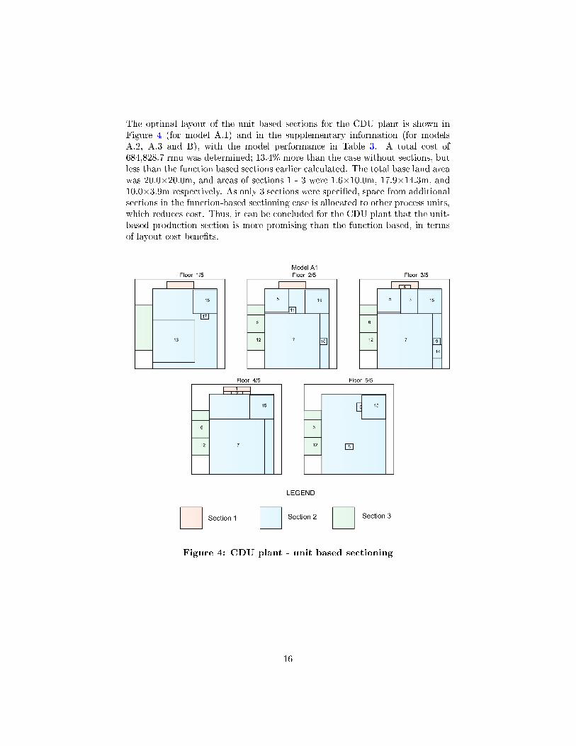
The optimal layout of the unit based sections for the CDU plant is shown inFigure 4 (for model A.1) and in the supplementary information (for modelsA.2, A.3 and B), with the model performance in Table 3. A total cost of684,828.7 rmu was determined; 13.4% more than the case without sections, butless than the function based sections earlier calculated. The total base land areawas 20.0×20.0m, and areas of sections 1 - 3 were 1.6×10.0m, 17.9×14.3m, and10.0×3.9m respectively. As only 3 sections were speci�ed, space from additionalsections in the function-based sectioning case is allocated to other process units,which reduces cost. Thus, it can be concluded for the CDU plant that the unit-based production section is more promising than the function-based, in termsof layout cost bene�ts.

Figure 4: CDU plant - unit based sectioning

16

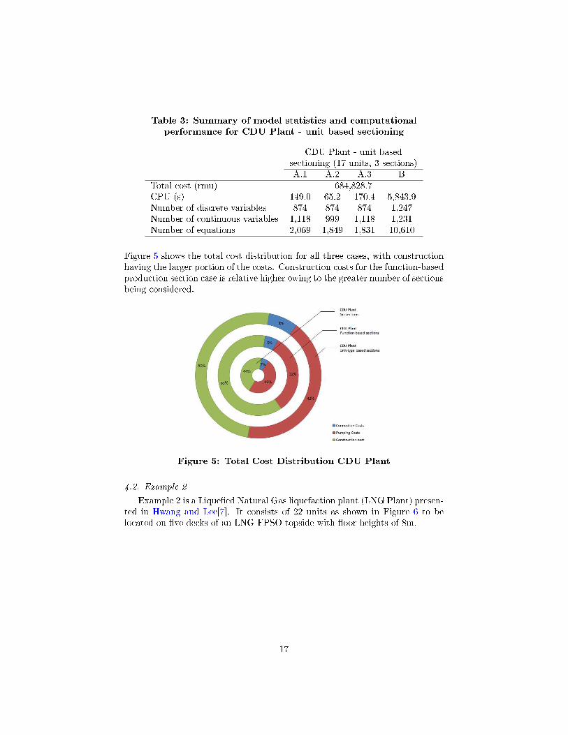
Table 3: Summary of model statistics and computationalperformance for CDU Plant - unit based sectioning

CDU Plant - unit basedsectioning (17 units, 3 sections)A.1 A.2 A.3 B

Total cost (rmu) 684,828.7CPU (s) 149.0 65.2 170.4 5,843.9Number of discrete variables 874 874 874 1,247Number of continuous variables 1,118 999 1,118 1,231Number of equations 2,069 1,849 1,831 10,610

Figure 5 shows the total cost distribution for all three cases, with constructionhaving the larger portion of the costs. Construction costs for the function-basedproduction section case is relative higher owing to the greater number of sectionsbeing considered.

Figure 5: Total Cost Distribution CDU Plant

4.2. Example 2

Example 2 is a Lique�ed Natural Gas liquefaction plant (LNG Plant) presen-ted in Hwang and Lee[7]. It consists of 22 units as shown in Figure 6 to belocated on �ve decks of an LNG-FPSO topside with �oor heights of 8m.

17

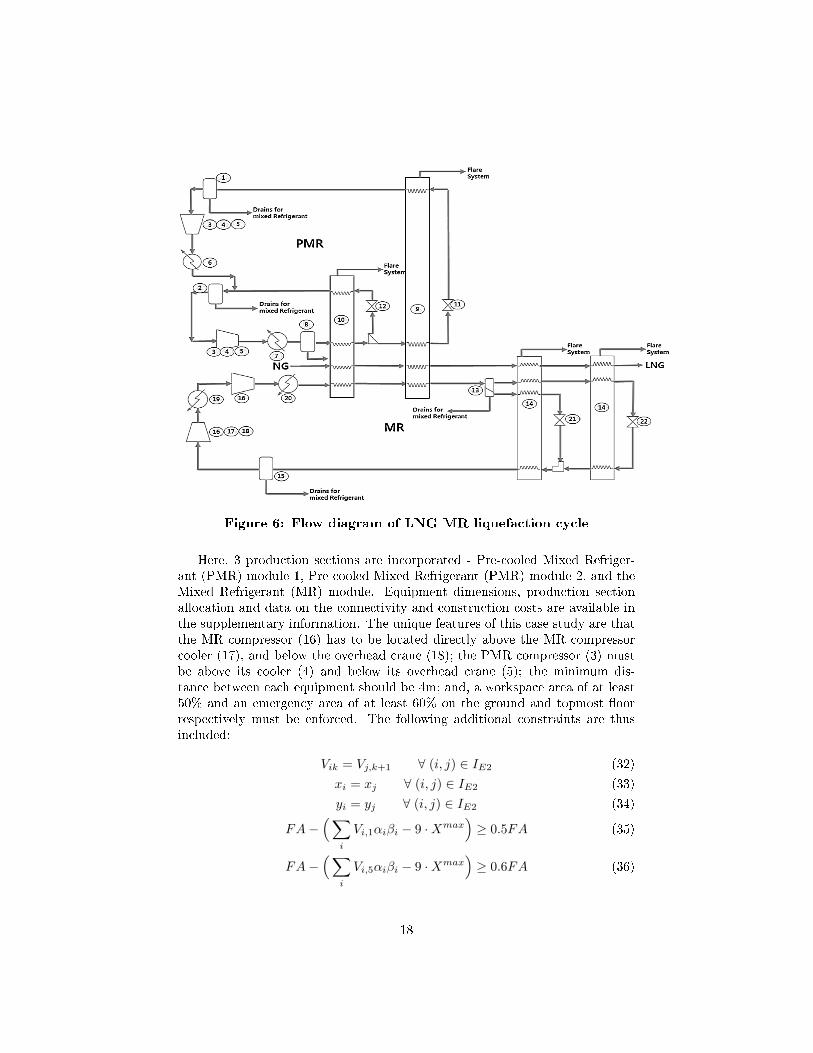
Figure 6: Flow diagram of LNG MR liquefaction cycle

Here, 3 production sections are incorporated - Pre-cooled Mixed Refriger-ant (PMR) module 1, Pre-cooled Mixed Refrigerant (PMR) module 2, and theMixed Refrigerant (MR) module. Equipment dimensions, production sectionallocation and data on the connectivity and construction costs are available inthe supplementary information. The unique features of this case study are thatthe MR compressor (16) has to be located directly above the MR compressorcooler (17), and below the overhead crane (18); the PMR compressor (3) mustbe above its cooler (4) and below its overhead crane (5); the minimum dis-tance between each equipment should be 4m; and, a workspace area of at least50% and an emergency area of at least 60% on the ground and topmost �oorrespectively must be enforced. The following additional constraints are thusincluded:

Vik = Vj,k+1 ∀ (i, j) ∈ IE2 (32)

xi = xj ∀ (i, j) ∈ IE2 (33)

yi = yj ∀ (i, j) ∈ IE2 (34)

FA−(∑

i

Vi,1αiβi − 9 ·Xmax)≥ 0.5FA (35)

FA−(∑

i

Vi,5αiβi − 9 ·Xmax)≥ 0.6FA (36)

18

where IE2 = {(3, 5), (4, 3), (16, 18), (17, 16)}. Equations (32) - (34) enforce therelative equipment positioning. Equations (35) and (36) are applied to eachsection and ensure that a portion of the area on the �rst and last �oor is leftfree by at least 50% and 60% of the total �oor area for the workspace and emer-gency area respectively. This total �oor area is taken as the area available forequipment layout plus an additional free area of Xmax×9m [7].The example was �rstly solved without production section considerations, andthe solution is summarised in Table 4. Each of models A.1 - B did not obtaina globally optimal solution at the time limit of 10,000s. Model A.2 however,proved to be the most computationally e�cient with a cost value of 1,466,654.2rmu - with 4%, 35% and 61% attributed to connection, pumping and con-struction costs respectively. A �oor area of 30.0×35.0m for 5 total �oors wascalculated.

Table 4: Summary of model statistics and computationalperformance for LNG Plant - no sections

LNG Liquefaction (22 units)A.1 A.2 A.3 B

Total cost (rmu) 1,466,654.2 1,563,086.2

CPU (s)10,000

(3.7%)1 (2.4%)1 (3.7%)1 (26.0%)1

Number of discrete variables 732 732 732 1,398Number of continuous variables 890 780 890 1,011Number of equations 2,990 2,778 2,770 10,734

1Relative gap quoted at CPU limit of 10,000s

The layout plots in Figure 7 (and in the supplementary information) showedthat all models were able to incorporate the additional considerations requiredin the example of relative equipment positioning, additional space provision(for emergency and maintenance activities at the desired �oors) and minimumequipment spacing. Furthermore, model B, unlike models A.1 - A.3, can modelcases of multi-�oor equipment that have varying dimensions (length, breadth ordiameter) at di�erent �oors, owing to an irregular shape (e.g. a Fluid CatalyticCracking (FCC) unit) or the presence of varying amounts of process unit aux-iliaries per �oor.It can also be observed from Figure 7 that equipment items are located irre-spective of the function they perform. For example, the PMR LP suction drum(1) is well isolated from its compressor - 3 - and other equipment (2 - 7) in thePMR module 1. This can reduce the e�ciency of maintenance activities for thePMR compressor, as well as process control operations for the PMR module 1.

19

Figure 7: LNG Plant layout results - no sections

20

Considering the 3 production sections/modules, the statistics of the proposedmodels are shown in Table 5. A total cost of 1,690,372.9 rmu representing a15% increase in comparison with its base case was obtained, with a base landarea of 35.0×40.0m. However, layout results showed that �oors 4 and 5 do notneed to be constructed in the PMR Module 1. The PMR module 1 had a �oorarea of 22.8×18.9m, PMR module 2 - 4.4×17.5m and MR module - 33.4×17.1m.Models A solved in times below 15 minutes, achieving global optimality, whileModel B, owing to the greater number of decision variables did not achieveglobal optimality by the time limit of 10,000 seconds.

Table 5: Summary of model statistics and computationalperformance for LNG Plant with production sections

LNG Liquefaction with productionsections (22 units)

A.1 A.2 A.3 BTotal cost (rmu) 1,690,372.9CPU (s) 683.1 883.2 700.2 10,000 (0.6%)1

Number of discrete variables 872 872 872 1,164Number of continuous variables 1,209 1,099 1,209 1,330Number of equations 2,312 2,100 2,092 9,308

1Relative gap quoted at CPU limit of 10,000s

The optimal layout is shown in Figure 8. Besides satisfying the minimumequipment spacing requirement and relative positioning, all models obtainedlayouts that allowed for well-de�ned production sections. These production sec-tions occupy a common area over an optimal number of �oors.

21

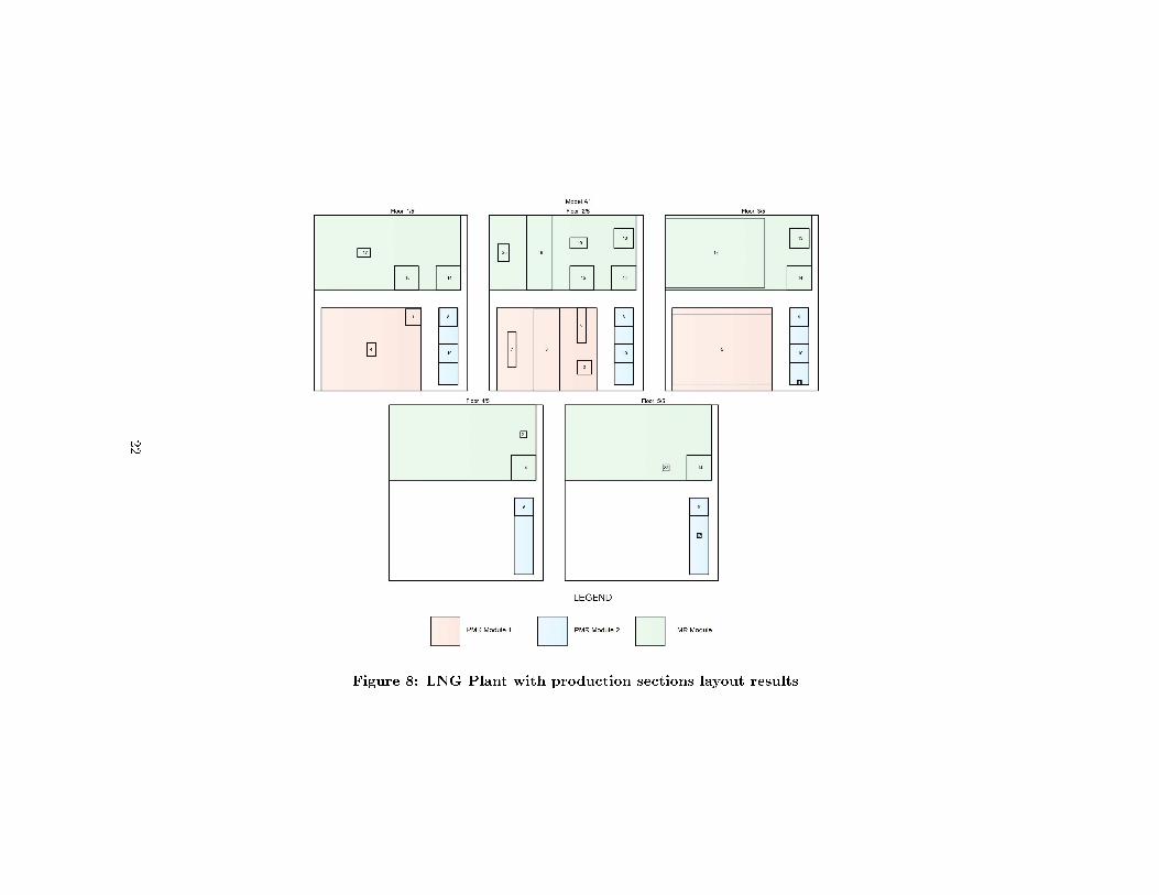
Figure 8: LNG Plant with production sections layout results

22

The total cost statistic is shown in Figure 9 for the layout with produc-tion sections. Construction costs are relatively higher due to additional spacerequirements for equipment segregations. This is observed in both examplesinvestigated, where the total plant layout costs with production sections werehigher than without them. However, due to other bene�ts in the areas of plantsafety, operability, maintenance and workforce management, etc., having pro-duction sections with pre-de�ned equipment is still common practice for plantlayout in the industry.

Figure 9: Total Cost Distribution (LNG Liquefaction plant withproduction sections)

5. Concluding remarks

An extension of the plant layout models by Ejeh et al. [2] was proposedto account for production sections in multi-�oor chemical process plants hav-ing tall/multi-�oor equipment. Additional constraints were included in all fourmodels (A.1, A.2, A.3 and B) to account for equipment allocated to di�er-ent production sections. These models simultaneously determined the optimalarrangement of production sections amongst one another (site layout), the ar-rangement of equipment in each production section (plot layout), as well as thenumber of �oors per section, �oor areas and total cost values considering pump-ing, connection, and construction costs.Two case studies were presented to highlight model applicability and perform-ance. Each case study was solved using the models in Ejeh et al. [2] as a basecase (without production sections) and then with the proposed models. Theresults showed that in both cases, the feature of production sections cannotbe achieved by the models in Ejeh et al. [2]. In the �rst case study - a CDU

23

plant - two criteria on production section allocation were adopted. For the �rstcriterion, equipment was placed in production sections based on the collectivefunction performed, and for the second, production sections were based on theindividual properties of the equipment, with the second being more cost e�ect-ive. In both cases, an increase in layout costs compared with the base casewas realised due to increased space requirements for production sections. Also,most of the proposed models achieved global optimality well under 10 minutes.The second and larger case study - LNG liquefaction plant - with 22 units in3 production sections also gave a higher cost with production sections. ModelsA reached global optimality under 15 minutes, with layout results giving anoptimal number of �oors per section.From the case studies, it was observed that the optimisation models with pro-duction sections outperform the models without them in terms of computationale�ciency. This, combined with the development of decomposition techniquesmay lead to more e�cient solutions for larger case studies.

Acknowledgement

JOE gratefully acknowledges the Petroleum Technology Development Fund(PTDF), Nigeria.

24

Appendix A. Optimal Multi-�oor process plant layout without pro-duction sections models

The four models proposed by Ejeh et al. [2] are presented as follows:

Nomenclature

Additional symbols used are de�ned as follows:

Parameters

αi, βi,γi dimensions of equipment item iIPij distance between the base and input point on item j

for the connection between items i and jOPij distance between the base and output point on equipment i

for the connection between items i and j

Integer variables

NF number of �oors

Binary variables

E1ij , E2ij non-overlapping binary, a set of values which prevents equipmentoverlap in one direction in the x-y plane

N ′ijk 1 if items i and j are assigned to �oor k; 0, otherwise

Oi 1 if length of item i is equal to αi; 0, otherwiseQs 1 if rectangular area s is selected for the layout; 0, otherwise

Sfik 1 if item i terminates on �oor k; 0, otherwiseWk 1 if �oor k is occupied; 0, otherwise

Continuous variables

ARs prede�ned rectangular �oor area sDij relative distance in z coordinates between items i and j,

if i is lower than jhi height of item iNQs linearisation variable expressing the product of NF and QsUij relative distance in z coordinates between items i and j,

if i is higher than jzi relative coordinate on the z-axis of the geometrical centre of item i

25

A.1. Model A.1

A.1.1. Floor constraints

∑k

Vik =Mi ∀ i (S.1)

N ′ijk ≥ Vik + Vjk − 1 ∀ i, j > i, k (S.2)

Nij ≥ N ′ijk ∀ i, j > i, k (S.3)

Ssik ≤Wk ∀ i, k (S.4)

Wk ≤Wk−1 ∀ k > 1; (S.5)

NF ≥∑k

Wk ∀ i (S.6)

A.1.2. Equipment orientation constraints

A 900 rotation of equipment orientation is allowed in the x-y plane.

li = αiOi + βi(1−Oi) ∀ i (S.7)

di = αi + βi − li ∀ i (S.8)

A.1.3. Multi-�oor equipment constraints

Multi-�oor equipment is modelled as follows:

−Vik + Vi,k−1 + Ssik ≥ 0 ∀i, k (S.9)

−Vik + Vi,k+1 + Sfik ≥ 0 ∀i, k (S.10)∑k

Ssik = 1 ∀i (S.11)∑k

Sfik = 1 ∀i (S.12)

k′+Mi−1∑k=k′

Vik′ ≥Mi.Ssik ∀i, k (S.13)

26

A.1.4. Non-overlapping constraints

To prevent two or more equipment items occupying the same space withina �oor, the following constraints are introduced:

xi − xj +BM(1−Nij + E1ij + E2ij) ≥li + lj

2+Deminij ∀ i, j > i (S.14)

xj − xi +BM(2−Nij − E1ij + E2ij) ≥li + lj

2+Deminij ∀ i, j > i (S.15)

yi − yj +BM(2−Nij + E1ij − E2ij) ≥di + dj

2+Deminij ∀ i, j > i

(S.16)

yj − yi +BM(3−Nij − E1ij − E2ij) ≥di + dj

2+Deminij ∀ i, j > i

(S.17)

A.1.5. Distance constraints

Distance constraints determine the relative distances in the x and y coordin-ates between connected equipment.

Rij − Lij = xi − xj ∀ i, j : fij = 1 (S.18)

Aij −Bij = yi − yj ∀ i, j : fij = 1 (S.19)

Uij −Dij = FH∑k

(k − 1)(Ssik − Ssjk) + OPij − IPij ∀ i, j : fij = 1

(S.20)

TDij = Rij + Lij +Aij +Bij + Uij +Dij ∀ i, j : fij = 1 (S.21)

A.1.6. Area Constraints

The area of each �oor is as described by equations (S.22) - (S.27).

FA =∑s

ARsQs (S.22)∑s

Qs = 1 (S.23)

The �oor length and depth is selected from the chosen rectangular area sizedimensions:

Xmax =∑s

XsQs (S.24)

Y max =∑s

Y sQs (S.25)

NQs ≤ K ·Qs ∀s (S.26)

NF =∑s

NQs (S.27)

27

A.1.7. Layout design constraints

Layout design constraints ensure that equipment items are placed within theboundaries of the �oor area and start from the base of a �oor.

xi ≥li2

∀ i (S.28)

yi ≥di2

∀ i (S.29)

xi +li2≤ Xmax ∀ i (S.30)

yi +di2≤ Y max ∀ i (S.31)

zi =hi2

∀ i (S.32)

A.1.8. Symmetry breaking constraints

Symmetry breaking constraints are introduced as follows:

xi + yi − xj − yj ≥ δ ·Nij ∀ (i, j) = argmaxi,j∈MF

Ccij (S.33)

E1ij = 0 ∀ (i, j) = argmaxi,j∈MF

Ccij (S.34)

where δ = min(li2 ,

di2

)+ min

(lj2 ,

dj2

). These �x the relative position of i to

j. Units i and j are chosen as the two multi-�oor units having the highestconnection costs.

A.1.9. Objective function

min∑i

∑j 6=i:fij=1

[CcijTDij + CvijDij + Chij(Rij + Lij +Aij +Bij)]

+FC1 ·NF + FC2∑s

ARs ·NQs + LC · FA(S.35)

subject to (S.1) - (S.34).

A.2. Model A.2

Model A.2 has the same formulation as A.1 with the exception that equations(S.10), (S.12) and (S.13) are replaced by (S.36) below:

Mi−1∑θ=1

Vi,k+θ ≥ (M i − 1).(Vik − Vi,k−1) ∀i, k (S.36)

A.3. Model A.3

For Model A.3, equations (S.9), (S.10) and (S.13) in model A.1 are replacedby (S.37) below:

Vik − Vi,k−1 = Ssik − Sfi,k−1 ∀i, k (S.37)

28

A.4. Model B

A.4.1. Floor constraints

∑k

Vi′k = 1 ∀ i′ (S.38)

Ni′j′ ≥ Vi′k + Vj′k − 1 ∀ i′, j′ > i′, k (S.39)

Ni′j′ ≤ 1− Vi′k + Vj′k ∀ i′, j′ > i′, k (S.40)

Ni′j′ ≤ 1 + Vi′k − Vj′k ∀ i′, j′ > i′, k (S.41)

Vi′k ≤Wk ∀ i′, k (S.42)

Wk ≤Wk−1 ∀ k = 2, ...,K (S.43)

NF ≥∑k

Wk (S.44)

A.4.2. Multi-�oor equipment constraint

Vi′k = Vi′−1,k−1 ∀ i′ ∈ Pi, k (S.45)

xi′ = xi′+1 ∀ i′ ∈ Pi (S.46)

yi′ = yi′+1 ∀ i′ ∈ Pi (S.47)

Oi′ = Oi′+1 ∀ i′ ∈ Pi (S.48)

A.4.3. Distance constraints

Ui′j′−Di′j′ = FH∑k

(k−1)(Vi′k−Vj′k)+OPi′j′−IPi′j′ ∀ i′, j′ ∈ I ′ : fi′j′ = 1

(S.49)

A.4.4. Objective function

min∑i′

∑j′ 6=i′:fi′j′=1

[Cci′j′TDi′j′ + Cvi′j′Di′j′ + Chi′j′(Ri′j′ + Li′j′ +Ai′j′ +Bi′j′)]

+FC1.NF + FC2∑s

ARs.NQs + LC.FA

(S.50)

subject to (S.7), (S.8), (S.14) - (S.19), (S.21) - (S.34) and (S.38) - (S.49).

29

References

[1] Barbosa-Póvoa, A. P., Mateus, R., Novais, A. Q., 2002. Optimal 3D layoutof industrial facilities. International Journal of Production Research 40 (7),1669�1698.

[2] Ejeh, J. O., Liu, S., Chalchooghi, M. M., Papageorgiou, L. G., 2018. Anoptimisation-based approach for process plant layout (under review).

[3] Furuholmen, M., Glette, K., Hovin, M., Torresen, J., 2010. A Coevolution-ary, Hyper Heuristic approach to the optimization of Three-dimensionalProcess Plant Layouts - A comparative study. IEEE Congress on Evolu-tionary Computation, 1�8.

[4] Georgiadis, M., Macchietto, S., 1997. Layout of process plants: A novelapproach. Computers & Chemical Engineering 21, S337�S342.

[5] Guirardello, R., Swaney, R. E., 2005. Optimization of process plant layoutwith pipe routing. Computers & Chemical Engineering 30 (1), 99�114.

[6] Hosseini-Nasab, H., Fereidouni, S., Fatemi Ghomi, S. M. T., Fakhrzad,M. B., 2018. Classi�cation of facility layout problems: a review study. In-ternational Journal of Advanced Manufacturing Technology 94 (1-4), 957�977.

[7] Hwang, J., Lee, K. Y., 2014. Optimal liquefaction process cycle consideringsimplicity and e�ciency for LNG FPSO at FEED stage. Computers andChemical Engineering 63 (63), 1�33.

[8] Kheirkhah, A., Navidi, H., Messi Bidgoli, M., 2015. Dynamic facility lay-out problem: a new bilevel formulation and some metaheuristic solutionmethods. IEEE Transactions on Engineering Management 62 (3), 396�410.

[9] Ku, N., Jeong, S.-Y., Roh, M.-I., Shin, H.-K., Ha, S., Hong, J.-W., 2014.Layout Method of a FPSO (Floating, Production, Storage, and O�-LoadingUnit) Using the Optimization Technique. In: Volume 1B: O�shore Tech-nology. ASME, pp. 1�11.

[10] Ku, N.-K., Hwang, J.-H., Lee, J.-C., Roh, M.-I., Lee, K.-Y., 2014. Optimalmodule layout for a generic o�shore LNG liquefaction process of LNG-FPSO. Ships and O�shore Structures 9 (3), 311�332.

[11] McCarl, B., Meeraus, A., Van der Eijk, P., Bussieck, M., Dirkse, S., Ne-lissen, F., 2017. Mccarl expanded gams user guide version 24.6. GAMSDevelopment, Washington, DC.

[12] Mecklenburgh, J., 1985. Process plant layout, 2nd Edition. Longman, NewYork.

30

[13] Medina-Herrera, N., Jiménez-Gutiérrez, A., Grossmann, I. E., 2014. Amathematical programming model for optimal layout considering quant-itative risk analysis. Computers and Chemical Engineering 68, 165�181.

[14] Moran, S., 2016. Engineering Practice Process Plant Layout - Becoming aLost Art? Chemical Engineering 123 (12), 71�76.

[15] Nabavi, S. R., Taghipour, A. H., Mohammadpour Gorji, A., 2016. Op-timization of Facility Layout of Tank farms using Genetic Algorithm andFireball Scenario. Chemical Product and Process Modeling 11 (2).

[16] Navidi, H., Bashiri, M., Bidgoli, M. M., 2012. A heuristic approach onthe facility layout problem based on game theory. International Journal ofProduction Research 50 (6), 1512�1527.

[17] Papageorgiou, L. G., Rotstein, G. E., 1998. Continuous-domain mathem-atical models for optimal process plant layout. Industrial & EngineeringChemistry Research 5885 (9), 3631�3639.

[18] Park, P. J., Lee, C. J., 2015. The Research of Optimal Plant Layout Optim-ization based on Particle Swarm Optimization for Ethylene Oxide Plant.Journal of the Korean Society of Safety 30 (3), 32�37.

[19] Patsiatzis, D. I., Papageorgiou, L. G., 2002. Optimal multi-�oor processplant layout. Computers & Chemical Engineering 26 (4), 575�583.

[20] Patsiatzis, D. I., Papageorgiou, L. G., 2003. E�cient Solution Approachesfor the Multi�oor Process Plant Layout Problem. Industrial & EngineeringChemistry Research 42 (4), 811�824.

[21] Penteado, F. D., Ciric, A. R., 1996. An MINLP Approach for Safe ProcessPlant Layout. Industrial & Engineering Chemistry Research 35 (4), 1354�1361.

[22] Peters, M. S., Timmerhaus, K. D., 2003. Plant Design and Economics forChemical Engineers. Vol. 4. McGraw-Hill New York.

[23] Xin, P., Khan, F., Ahmed, S., 2016. Layout Optimization of a FloatingLique�ed Natural Gas Facility Using Inherent Safety Principles. Journal ofO�shore Mechanics and Arctic Engineering 138 (4), 041602.

[24] Xu, G., Papageorgiou, L. G., 2009. Process plant layout using animprovement-type algorithm. Chemical Engineering Research and Design87 (6), 780�788.

31