optimal estimation of suspended-sediment concentrations in ... · us geological survey, water...
TRANSCRIPT

HYDROLOGICAL PROCESSESHydrol. Process. 15, 1133–1155 (2001)DOI: 10.1002/hyp.207
Optimal estimation of suspended-sedimentconcentrations in streams
David J. Holtschlag*US Geological Survey, Water Resources Division, 6520 Mercantile Way, Suite 5, Lansing, MI 48911, USA
Abstract:
Optimal estimators are developed for computation of suspended-sediment concentrations in streams. The estimatorsare a function of parameters, computed by use of generalized least squares, which simultaneously account for effectsof streamflow, seasonal variations in average sediment concentrations, a dynamic error component, and the uncertaintyin concentration measurements. The parameters are used in a Kalman filter for on-line estimation and an associatedsmoother for off-line estimation of suspended-sediment concentrations. The accuracies of the optimal estimators arecompared with alternative time-averaging interpolators and flow-weighting regression estimators by use of long-termdaily-mean suspended-sediment concentration and streamflow data from 10 sites within the United States. For samplingintervals from 3 to 48 days, the standard errors of on-line and off-line optimal estimators ranged from 52Ð7 to 107%, andfrom 39Ð5 to 93Ð0%, respectively. The corresponding standard errors of linear and cubic-spline interpolators rangedfrom 48Ð8 to 158%, and from 50Ð6 to 176%, respectively. The standard errors of simple and multiple regressionestimators, which did not vary with the sampling interval, were 124 and 105%, respectively. Thus, the optimal off-lineestimator (Kalman smoother) had the lowest error characteristics of those evaluated. Because suspended-sedimentconcentrations are typically measured at less than 3-day intervals, use of optimal estimators will likely result insignificant improvements in the accuracy of continuous suspended-sediment concentration records. Additional researchon the integration of direct suspended-sediment concentration measurements and optimal estimators applied at hourlyor shorter intervals is needed.
KEY WORDS suspended sediments; optimal estimation; Kalman filtering; computation; flux; loads
INTRODUCTION
Since 1995, the National Stream Quality Accounting Network (NASQAN) of the US Geological Survey(USGS) has monitored water quality at 40 stations on four of the nation’s largest basins, including theColumbia, the Colorado, the Mississippi, and the Rio Grande. Monitored constituents include sedimentconcentrations, major ions, trace elements, nutrients, pesticides, carbon, and support variables includingstreamflow, dissolved oxygen, temperature, pH, and conductivity. To ensure that these data are used aseffectively as possible, the NASQAN programme, through the USGS Office of Water Quality, has supportedthe development of optimal estimators of suspended-sediment concentrations. The general form of theseestimators may also be applicable to other constituents.
Sediment in streams results from erosion in the basin and transport by flowing water (Guy, 1970).Either process can limit the occurrence of sediment in streams. Total sediment discharge includes a bed-load component and a suspended-sediment component. Bed load refers to sediment particles rolling, sliding,or tumbling along the streambed. Suspended sediment represents that component of sediment that stays insuspension for an appreciable length of time and represents a dynamic equilibrium between the upward forcesof turbulence holding particles in suspension against the downward force of gravity. Turbulent forces are
* Correspondence to: D. J. Holtschlag, US Geological Survey, Water Resources Division, 6520 Mercantile Way, Suite 5, Lansing, MI 48911,USA. E-mail: [email protected]
Received 15 November 1999This article is a US government work and is in the public domain in the United States Accepted 15 May 2000

1134 D. J. HOLTSCHLAG
directly related to streamflow rate, and the effectiveness of gravitational forces is related to particle sizes anddensities. In most natural rivers, sediments are transported mainly as suspended sediment (Yang, 1996).
Estimation of average sediment concentrations and flux rates requires the integration of continuous data onstreamflow with discrete measurements of sediment concentration. This integration is commonly carried outby interpolating discrete measurements by use of time-averaging or flow-weighting methods. Phillips et al.,(1999) compared 20 existing and two proposed methods for computing loads and found that a time-averagingmethod produced the most precise estimates for two stations analysed. The precision of this method decreasessignificantly, however, as the sampling interval increases (Phillips et al., 1999). Furthermore, Bukaveckaset al. (1998) conclude that time-averaging methods may produce biased estimates of flux during periods ofvariable discharge.
A sediment-rating curve approach (Helsel and Hirsch, 1992) is a common method of flow weighting.This type of rating curve generally describes the relation between the logs [where log refers to thecommon (base 10) logarithm function] of suspended-sediment concentration and the logs of streamflow.This rating-curve approach, however, has been found to underestimate river loads (Ferguson, 1986). Inaddition, Bukaveckas et al. (1998) indicate that flow-weighting methods may produce biased estimates if theconcentration–streamflow relation is affected by antecedent conditions or has seasonal variability. Seasonalrating curves are used to reduce the scatter and to eliminate this bias at some sites (Yang, 1996). Althoughbeyond the scope of this study, Richards and Holloway (1987) evaluate the accuracy and precision of tributaryload estimates as affected by both sampling frequency and pattern.
The concentrations of suspended sediments are measured at stream-gauging stations throughout the UnitedStates because of the environmental and economic significance of the effect of sediment on receiving waters.The USGS operates many of these stations, which are funded through several cooperative and federalprogrammes. Daily-mean concentrations of suspended sediment are determined for sites where sufficient directmeasurements of suspended-sediment concentration and continuous streamflow data are available (RandyParker, US Geological Survey, written communication, 1999). Because of the uniform data-collection methods(Guy and Norman, 1973) and computational procedures (Porterfield, 1972; Glysson, 1987) used by the USGS,these data provide the best available information on suspended-sediment flux in the nation’s rivers. In addition,the USGS maintains a nationwide database of suspended-sediment concentration, streamflow, and ancillarydata (Randy Parker, written communication, 1999). The database contains daily values for 1593 stations inthe United States that have an average period of record of 5Ð3 years. This database was used for the analysisreported in this paper and is accessible from the Internet at http://webserver.cr.usgs.gov/sediment/
Purpose and scope
This paper develops optimal on-line and off-line estimators of suspended-sediment concentrations forstreams on the basis of daily values of computed suspended-sediment concentration and streamflow infor-mation. Data from 10 sites are used to compare the accuracy of the optimal estimators with interpolationand regression estimators (Koltun et al., 1994) that are commonly used to compute suspended-sedimentconcentration records. The estimators were restricted to those that could be readily implemented withdata that are generally available at gauging stations. The choice of daily-value rather than unit-value(hourly or less) computational intervals, however, was based on the greater accessibility of daily-valuedata. The optimal estimators developed in this paper are intended for eventual application at unit-valueintervals.
Site selection
Ten USGS gauging stations (Figure 1, Table I) were selected to develop the estimators and assess theiraccuracy. The sites represent a broad range of basin sizes, suspended-sediment concentration characteristics,and streamflow characteristics. Basin drainage areas range from 1610 to 116 000 km2. Median suspended-sediment concentrations (Figure 2) range from 8 to 3040 mg/l. Median streamflow (Figure 3) ranged from
Published in 2001 by John Wiley & Sons, Ltd. Hydrol. Process. 15, 1133–1155 (2001)

OPTIMAL ESTIMATION OF SUSPENDED-SEDIMENT CONCENTRATIONS 1135
Figure 1. Locations of selected US Geological Survey sediment gauging stations in the United States
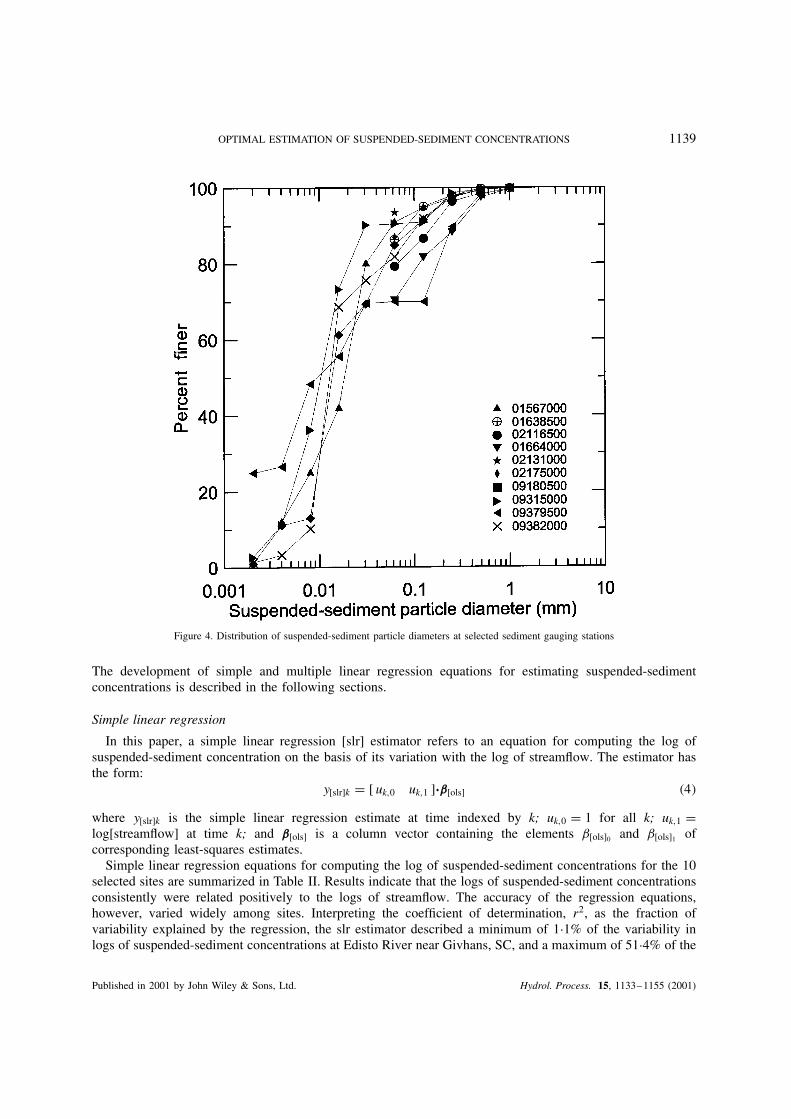
0Ð34 to 241 m3/s. Available suspended-sediment particle-size distribution data indicates that the percentageof suspended sediment finer than 0Ð125 mm ranged from 70 to 95% (Figure 4) among sites.
ESTIMATORS OF SUSPENDED-SEDIMENT CONCENTRATIONS
Previous estimators for computing records of suspended-sediment concentrations (Koltun et al., 1994) includeboth time-averaging and flow-weighting procedures. In this paper, time-averaging procedures refer to linear orcubic-spline interpolators between direct suspended-sediment concentration measurements, typically obtainedat unequal time intervals. These estimators have no rigorous mechanism for quantifying the uncertainty of thevalues produced, but provide estimates that are consistent with data at the times of direct measurements.Flow-weighting procedures include linear regressions, which condition estimates of suspended-sedimentconcentrations on streamflow (and sometimes other explanatory variables). The regression estimators accountfor a primary source of variability between measurements of sediment concentration and provide a measureof uncertainty. Regression estimators, however, do not converge appropriately to measured values at timesof direct measurement. Optimal estimators combine the benefits of both time-averaging and flow-weightingprocedures in a formal mathematical model that also describes the statistical uncertainty in the estimates.
Both suspended-sediment concentrations and streamflow tend to be highly skewed to the right. Logarithmic(log) transformation, however, creates a more symmetrical distribution (Figure 5). The linearity betweenpercent frequency, on a normal probability scale, and both suspended-sediment concentrations (Figure 2)and streamflow (Figure 3), on the log scale, supports the common assumption that suspended-sedimentconcentrations and streamflow are approximately log-normally distributed. The log transformation improveslinearity between the sediment concentrations and streamflow (Figure 6) and reduces heteroscedasticity(nonconstant variance that may be a function of magnitude) in the model errors. Thus, interpolation andregression methods generally apply a log transformation prior to method application. In addition, someestimators provide an adjustment for the seasonal variations (Figure 7) in average sediment concentrations.
Published in 2001 by John Wiley & Sons, Ltd. Hydrol. Process. 15, 1133–1155 (2001)

1136 D. J. HOLTSCHLAG
Tabl
eI.
Iden
tifica
tion
and
loca
tion
ofse
lect
edse
dim
ent
gaug
ing
stat
ions
US
GS
stat
ion
Stat
ion
nam
eB
asin
area
Lat
itud
eL
ongi
tude
Dat
eof
the
Dat
eof
the
Pro
cess
vari
ance
,Qk
num
ber
(km
2)
begi
nnin
gof
the
endi
ngof
the
for
a1-
day
tim
est
eppe
riod
ofre
cord
peri
odof
reco
rdco
mpu
ted
wit
ha
used
inan
alys
isus
edin
anal
ysis
mea
sure
men
ter
ror
vari
ance
ofR
D0Ð0
4an
dP
0C
D1
0156
7000
Juni
ata
Riv
erat
New
port
,PA
8687
40° 2
80 4200
77° 0
70 4600
July
29,
1952
Sept
.30
,19
890Ð1
357
0163
8500
Poto
mac
Riv
erat
Poin
tof
Roc
ks,
MD
2500
039
° 160 25
0077
° 320 35
00Ju
ly12
,19
66Se
pt.
30,
1990
0Ð101
501
6640
00R
appa
hann
ock
Riv
erat
Rem
ingt
on,
VA
1610
38° 3
10 5000
77° 4
80 5000
July
9,19
65Se
pt.
30,
1993
0Ð289
302
1165
00Y
adki
nR
iver
atY
adki
nC
olle
ge,
NC
5910
35° 5
10 2400
80° 2
30 1000
Jan.
3,19
51Se
pt.
30,
1989
0Ð142
102
1310
00Pe
eD
eeR
iver
atPe
edee
,SC
2290
034
° 120 15
0079
° 320 55
00Se
pt.
25,
1968
Sept
.30
,19
720Ð0
799
0217
5000
Edi
sto
Riv
erne
arG
ivha
ns,
SC70
7033
° 010 40
0080
° 230 30
00M
ar.
26,
1967
Sept
.30
,19
720Ð1
959
0918
0500
Col
orad
oR
iver
near
Cis
co,
UT
1640
038
° 480 38
0010
9°17
0 3400
May
1,19
68Se
pt.
30,
1984
0Ð166
509
3150
00G
reen
Riv
erat
Gre
enR
iver
,U
T11
600
038
° 590 10
0011
0°09
0 0200
Aug
.19
,19
68Se
pt.
30,
1984
0Ð102
509
3795
00Sa
nJu
anR
iver
near
Blu
ff,
UT
5960
037
° 080 49
0010
9°51
0 5100
Dec
.17
,19
51D
ec.
3,19
580Ð1
127
0938
2000
Pari
aR
iver
atL
ees
Ferr
y,A
Z36
5036
° 520 20
0011
1°35
0 3800
Oct
.1,
1948
Sept
.30
,19
760Ð5
496
Published in 2001 by John Wiley & Sons, Ltd. Hydrol. Process. 15, 1133–1155 (2001)

OPTIMAL ESTIMATION OF SUSPENDED-SEDIMENT CONCENTRATIONS 1137
Figure 2. Distribution of daily mean concentrations of suspended sediment at selected gauging stations
Interpolators
Interpolation provides a mechanism for time-averaging direct measurements. Both linear and nonlinearinterpolation is used to compute daily suspended-sediment concentrations from unequally-spaced measure-ments (Koltun et al., 1994). Interpolation provides estimates that match direct measurements of concentrationexactly at the time of measurement. Linear interpolation approximates concentrations between times ofdirect measurements as straight-line segments connecting log-transformed concentrations on linear timescales. Nonlinear interpolation is based on a cubic-spline function between log-transformed values on alinear time scale. This interpolation produces a continuously differentiable arc that approximates a manu-ally drawn curve. Estimates of concentrations from interpolations are obtained by inverse log transformation(exponentiation).
Regression estimators
Regression models can be used to flow-weight estimates of suspended-sediment concentration. Thesemodels describe a static statistical relation between suspended-sediment concentrations and the corre-sponding set of explanatory variables. Explanatory variables are selected based on their correlation withsuspended-sediment concentrations and their general availability. Once developed, regression equationsare used to estimate suspended-sediment concentrations during periods when direct measurements areunavailable.
Published in 2001 by John Wiley & Sons, Ltd. Hydrol. Process. 15, 1133–1155 (2001)

1138 D. J. HOLTSCHLAG
Figure 3. Distribution of daily mean streamflow rates at selected sediment gauging stations
The general form of a regression equation is:
yk D uk·b C εk �1
where yk is the log of the suspended-sediment concentration at time k. Suspended sediment concentrations,Yk , are commonly measured in milligrams per litre; uk is a (p C 1)-dimensional row vector of explanatoryvariables at time k, where p is the number of explanatory variables, with 1 added to provide an interceptterm; b is a (p C 1)-dimensional column vector of parameters; and εk is the regression residual at time k. Theset of residuals from regression equations is generally assumed to be independent and normally distributedwith a mean of zero and a variance of �2, commonly written as ε ¾ NI�0, �2.
In ordinary least-squares regression, the estimate of b, denoted bols, is computed as:
bols D �UT·U�1UTy �2
where the n ð �p C 1 matrix U is formed by horizontally concatenating n rows (observations) of the ukvectors. The superscript T indicates a matrix transpose and the superscript �1 indicates a matrix inversion.Finally, the regression estimate of suspended-sediment concentration for time indexed by k is computed as:
y[ols]k D uk·bols �3
Published in 2001 by John Wiley & Sons, Ltd. Hydrol. Process. 15, 1133–1155 (2001)
OPTIMAL ESTIMATION OF SUSPENDED-SEDIMENT CONCENTRATIONS 1139
Figure 4. Distribution of suspended-sediment particle diameters at selected sediment gauging stations
The development of simple and multiple linear regression equations for estimating suspended-sedimentconcentrations is described in the following sections.
Simple linear regression
In this paper, a simple linear regression [slr] estimator refers to an equation for computing the log ofsuspended-sediment concentration on the basis of its variation with the log of streamflow. The estimator hasthe form:
y[slr]k D [ uk,0 uk,1 ]·b[ols] �4
where y[slr]k is the simple linear regression estimate at time indexed by k; uk,0 D 1 for all k; uk,1 Dlog[streamflow] at time k; and b[ols] is a column vector containing the elements ˇ[ols]0 and ˇ[ols]1 ofcorresponding least-squares estimates.
Simple linear regression equations for computing the log of suspended-sediment concentrations for the 10selected sites are summarized in Table II. Results indicate that the logs of suspended-sediment concentrationsconsistently were related positively to the logs of streamflow. The accuracy of the regression equations,however, varied widely among sites. Interpreting the coefficient of determination, r2, as the fraction ofvariability explained by the regression, the slr estimator described a minimum of 1Ð1% of the variability inlogs of suspended-sediment concentrations at Edisto River near Givhans, SC, and a maximum of 51Ð4% of the
Published in 2001 by John Wiley & Sons, Ltd. Hydrol. Process. 15, 1133–1155 (2001)

1140 D. J. HOLTSCHLAG
Figure 5. Distribution of suspended-sediment concentrations and streamflow at Potomac River at Point of Rocks, MD
Figure 6. Relation between streamflow and suspended-sediment concentration at Juniata River at Newport, PA
Published in 2001 by John Wiley & Sons, Ltd. Hydrol. Process. 15, 1133–1155 (2001)

OPTIMAL ESTIMATION OF SUSPENDED-SEDIMENT CONCENTRATIONS 1141
Figure 7. Monthly variation in suspended-sediment concentrations at Potomac River at Point of Rocks, MD
variability in logs of suspended-sediment concentrations at Paria River at Lees Ferry, AZ. Residuals of all slrequations were highly autocorrelated as indicated by Durbin–Watson d-statistic values less than 2 (Table II),thus violating the assumption of independent residuals associated with ordinary least-squares regression.
Multiple linear regression
Relative to the simple linear regressions, multiple linear regression [mlr] equations increase the number ofexplanatory variables to improve the estimation accuracy. The form of this equation is:
y[mlr]k D [ uk,0 uk,1 uk,2 uk,3 uk,4 ]·b[ols] �5
where uk,0 and uk,1 are as defined previously; uk,2 D sin[2�·jk/366], where jk is the day number of the yearsuch that, in a leap year, j1 D 1 corresponds to January 1 and j366 D 366 corresponds to December 31;uk,3 D cos[2�·jk/366]; and uk,4 D �uk,1 � uk�1,1/�tk � tk�1, where tk is the time indexed by k. Together thenumerator and denominator provide an Euler approximation to the change in streamflow at time k. Againb[ols] is a column vector of corresponding ordinary least-squares parameter estimates.
The parameter estimates ˇ[ols]2 and ˇ[ols]3 describe a sinusoid of amplitude A and phase ϕ to approximatethe seasonal variability of log-transformed suspended-sediment concentrations. In particular, the amplitudeand phase parameters are computed as:
A D√ˇ2
[ols]2C ˇ2
[ols]3�6
ϕ D tan�1[ˇ[ols]3
ˇ[ols]2
]�7
and the resulting seasonal component can be written:
Sk D A sin[
2�·jk366
C ϕ
]�8
In the mlr equations (Table II), logs of streamflow were again positively associated with logs of suspended-sediment concentrations. In addition, with the exception of Paria River at Lees Ferry, AZ, positive changesin daily streamflow were associated with increasing suspended-sediment concentrations. Finally, a seasonalcomponent in logs of sediment concentrations was consistently detected at all sites. Conditioned on streamflow,the day of lowest average suspended-sediment concentrations was February 15 and the corresponding dayof highest average concentrations was August 17. The amplitude of the seasonal component varied from
Published in 2001 by John Wiley & Sons, Ltd. Hydrol. Process. 15, 1133–1155 (2001)

1142 D. J. HOLTSCHLAG
Tabl
eII
.M
odel
para
met
ers
and
sum
mar
yst
atis
tics
for
sele
cted
stat
ions
(slr
indi
cate
ssi
mpl
eli
near
regr
essi
on,
mlr
indi
cate
sm
ulti
ple
line
arre
gres
sion
,gl
sin
dica
tes
gene
rali
zed
leas
tsq
uare
s)
Stat
ion
nam
eE
quat
ion
Num
ber
Mod
elpa
ram
eter
esti
mat
esC
oeffi
cien
tof
Roo
tm
ean
Dub
in–
(sta
ndar
der
rors
)de
term
inat
ion:
squa
reer
ror
Wat
son
tota
l(p
arti
al)
d-st
atis
tic
ˇ0
ˇ1
ˇ2
ˇ3
ˇ4
�
Juni
ata
Riv
erat
New
port
,PA
slr
1357
6�1
Ð4181
0Ð850
6—
——
—0Ð4
814
0Ð885
70Ð2
225
(0Ð03
29)
(0Ð00
76)
mlr
�1Ð80
630Ð9
419
�0Ð18
55�0
Ð3678
0Ð800
0—
0Ð553
10Ð8
222
0Ð248
4(0
Ð0394
)(0
Ð0091
)(0
Ð0128
)(0
Ð0101
)(0
Ð0301
)gl
s�3
Ð2337
1Ð278
7�0
Ð4795
�0Ð41
760Ð2
405
�0Ð90
00(0
Ð4563
)0Ð3
782
2Ð016
0(0
Ð0762
)(0
Ð0163
)(0
Ð0474
)(0
Ð0454
)(0
Ð0149
)(0
Ð0037
)0Ð9
055
Poto
mac
Riv
erat
Poin
tof
Roc
ks,
MD
slr
8845
�0Ð60
540Ð6
757
——
——
0Ð311
50Ð9
375
0Ð165
7
(0Ð05
62)
(0Ð01
07)
mlr
�2Ð01
580Ð9
467
�0Ð45
04�0
Ð6860
0Ð651
1—
0Ð538
90Ð7
673
0Ð221
6(0
Ð0574
)(0
Ð0110
)(0
Ð0141
)(0
Ð0118
)(0
Ð0376
)gl
s�3
Ð8526
1Ð301
1�0
Ð7132
�0Ð76
560Ð1
427
�0Ð91
03(0
Ð4498
)0Ð3
371
1Ð902
4(0
Ð1056
)(0
Ð0189
)(0
Ð0572
)(0
Ð0558
)(0
Ð0188
)(0
Ð0044
)0Ð9
110
Rap
paha
nnoc
kR
iver
atR
emin
gton
,V
Asl
r10
309
0Ð839
40Ð7
193
——
——
0Ð451
60Ð9
564
0Ð412
1
(0Ð02
05)
(0Ð00
78)
mlr
0Ð584
90Ð8
266
�0Ð28
93�0
Ð3593
0Ð555
7—
0Ð533
50Ð8
823
0Ð427
4(0
Ð0226
)(0
Ð0089
)(0
Ð0145
)(0
Ð0128
)(0
Ð0224
)gl
s0Ð0
950
1Ð035
8�0
Ð4733
�0Ð43
860Ð2
585
�0Ð80
98(0
Ð4755
)0Ð5
331
2Ð159
9(0
Ð0473
)(0
Ð0164
)(0
Ð0414
)(0
Ð0395
)(0
Ð0135
)(0
Ð0058
)0Ð8
297
Yad
kin
Riv
erat
Yad
kin
Col
lege
,N
Csl
r14
149
�1Ð10
091Ð2
976
——
——
0Ð511
30Ð7
980
0Ð265
5
(0Ð04
51)
(0Ð01
07)
mlr
�1Ð85
051Ð4
760
�0Ð26
76�0
Ð6131
0Ð128
0—
0Ð674
30Ð6
516
0Ð390
7(0
Ð0419
)(0
Ð0099
)(0
Ð0086
)(0
Ð0078
)(0
Ð0203
)gl
s�1
Ð6176
1Ð420
3�0
Ð2469
�0Ð60
830Ð1
012
�0Ð80
59(0
Ð5373
)0Ð3
863
2Ð055
6(0
Ð0642
)(0
Ð0148
)(0
Ð0242
)(0
Ð0236
)(0
Ð0124
)(0
Ð0050
)0Ð8
855
Published in 2001 by John Wiley & Sons, Ltd. Hydrol. Process. 15, 1133–1155 (2001)

OPTIMAL ESTIMATION OF SUSPENDED-SEDIMENT CONCENTRATIONS 1143
Pee
Dee
Riv
erat
Peed
ee,
SCsl
r14
652Ð3
975
0Ð265
7—
——
—0Ð1
490
0Ð418
60Ð7
699
(0Ð09
12)
(0Ð01
66)
mlr
2Ð088
40Ð3
221
�0Ð10
76�0
Ð1825
0Ð618
7—
0Ð330
00Ð3
718
0Ð843
8(0
Ð0938
)(0
Ð0171
)(0
Ð0154
)(0
Ð0141
)(0
Ð0473
)gl
s1Ð5
565
0Ð419
4�0
Ð1476
�0Ð19
770Ð4
770
�0Ð59
77(0
Ð2739
)0Ð3
020
2Ð201
1(0
Ð1662
)(0
Ð0302
)(0
Ð0303
)(0
Ð0282
)(0
Ð0404
)(0
Ð0213
)0Ð5
584
Edi
sto
Riv
erne
arG
ivha
ns,
SCsl
r20
141Ð7
393
0Ð094
7—
——
—0Ð0
112
0Ð553
00Ð7
885
(0Ð08
14)
(0Ð01
98)
mlr
1Ð165
00Ð2
328
�0Ð18
21�0
Ð2372
0Ð453
5—
0Ð133
40Ð5
181
0Ð896
6(0
Ð0863
)(0
Ð0210
)(0
Ð0180
)(0
Ð0169
)(0
Ð1579
)gl
s1Ð1
594
0Ð234
4�0
Ð1824
�0Ð23
750Ð4
760
�0Ð55
15(0
Ð0458
)0Ð4
323
2Ð332
6(0
Ð1571
)(0
Ð0382
)(0
Ð0333
)(0
Ð0313
)(0
Ð2024
)(0
Ð0186
)0Ð3
970
Col
orad
oR
iver
near
Cis
co,
UT
slr
5995
�0Ð25
681Ð1
631
——
——
0Ð305
91Ð2
554
0Ð131
8
(0Ð11
51)
(0Ð02
26)
mlr
2Ð133
70Ð6
849
0Ð162
5�0
Ð8998
2Ð841
7—
0Ð460
71Ð1
069
0Ð196
7(0
Ð1204
)(0
Ð0238
)(0
Ð0213
)(0
Ð0232
)(0
Ð1688
)gl
s�5
Ð2931
2Ð162
8�0
Ð2003
†�0
Ð1957
†0Ð2
827
�0Ð95
250Ð1
892
0Ð436
01Ð9
313
(0Ð40
63)
(0Ð07
73)
(0Ð15
86)
(0Ð16
20)
(0Ð07
03)
(0Ð00
40)
0Ð916
4G
reen
Riv
erat
Gre
enR
iver
,U
Tsl
r58
850Ð3
445
1Ð162
4—
——
—0Ð3
857
0Ð959
30Ð1
343
(0Ð09
523)
(0Ð01
91)
mlr
2Ð591
80Ð7
069
0Ð224
8�0
Ð6401
0Ð880
2—
0Ð482
80Ð8
805
0Ð169
1(0
Ð1129
)(0
Ð0228
)(0
Ð0178
)(0
Ð0197
)(0
Ð1180
)gl
s0Ð2
314
1Ð185
60Ð0
693
�0Ð40
790Ð0
179†
�0Ð92
61(0
Ð1315
)0Ð3
451
1Ð778
4(0
Ð2720
)(0
Ð0537
)(0
Ð0853
)(0
Ð0882
)(0
Ð0480
)(0
Ð0049
)0Ð9
206
San
Juan
Riv
erne
arB
luff
,U
Tsl
r25
426Ð2
933
0Ð517
7—
——
—0Ð2
540
0Ð975
70Ð1
623
(0Ð06
49)
(0Ð01
76)
mlr
6Ð132
00Ð5
636
�0Ð22
430Ð0
075
0Ð647
7—
0Ð284
90Ð9
558
0Ð177
7(0
Ð0796
)(0
Ð0220
)(0
Ð0297
)(0
Ð0316
)(0
Ð0913
)gl
s3Ð6
322
1Ð274
3�0
Ð6377
†0Ð5
436†
�0Ð14
73�0
Ð9483
(0Ð31
65)
0Ð360
71Ð9
641
(0Ð20
51)
(0Ð04
34)
(0Ð18
71)
(0Ð18
75)
(0Ð03
55)
(0Ð00
63)
0Ð898
2Pa
ria
Riv
erat
Lee
sFe
rry,
AZ
slr
1022
58Ð4
937
1Ð995
0—
——
—0Ð5
144
1Ð920
60Ð2
317
(0Ð02
78)
(0Ð01
92)
mlr
9Ð044
12Ð5
180
�0Ð35
41�1
Ð2712
�1Ð01
68—
0Ð631
51Ð6
733
0Ð293
5(0
Ð0261
)(0
Ð0191
)(0
Ð0234
)(0
Ð0258
)(0
Ð0327
)gl
s7Ð8
562
1Ð386
4�0
Ð2789
�0Ð63
51�0
Ð2662
�0Ð91
91(0
Ð3736
)0Ð7
660
1Ð889
2(0
Ð0961
)(0
Ð0209
)(0
Ð1293
)(0
Ð1304
)(0
Ð0148
)(0
Ð0039
)0Ð9
228
†Pa
ram
eter
not
stat
istic
ally
sign
ifica
ntat
the
0Ð05
leve
l.
Published in 2001 by John Wiley & Sons, Ltd. Hydrol. Process. 15, 1133–1155 (2001)
1144 D. J. HOLTSCHLAG
a maximum of 1Ð0463 (in log of milligram per litre units) at Potomac River at Point of Rocks, MD, to aminimum of 0Ð2467 at Pee Dee River at Peedee, SC. Similar to the slr results, significant autocorrelation waspresent in the residuals of mlr estimates.
State-space estimators
State-space models provide a basis for optimal estimation, that is minimizing the error of the estimate ofthe state, by utilizing knowledge of system and measurement dynamics, assumed statistics of system noisesand measurement errors, and initial condition information (Gelb, 1974). State-space models disaggregatea dynamic system such as suspended-sediment concentrations into process and measurement components.The process component describes the evolution of the system dynamics and their associated uncertainty.The measurement component describes the static effects of explanatory variables and the uncertainty in themeasurement process. Together, these components form an estimator that continually accounts for the effectsof known inputs (such as streamflow) and optimally adjusts model estimates for periodic direct measurementsthat contain some uncertainty.
The process of adjusting for direct measurements is described as predicting, filtering, or smoothing,depending on the set of direct measurements used in estimation. Predicting uses only measurements priorto the time of estimation; filtering uses only measurements up to and including the time of estimation; andsmoothing uses measurements before and after the time of estimation. Predicted and filtered estimates provideon-line data, that is, information that can be continuously updated to the present (real time). Smoothedestimates provide off-line data only, that is, estimates are delayed until subsequent direct measurementsbecome available. The accuracy of off-line estimates, however, is generally greater than that of correspondingon-line values. The length of the delay is determined by measurement frequency. Both on-line and off-linesestimators will be developed and analysed in this paper, although the off-line estimators are of primary interestfor publication of suspended-sediment concentrations. In this paper, the state-space models are developed indiscrete, rather than continuous, time based on average values that are reported (sampled) at a time stepof 1 day. Thus, the state-space models are in the form of difference rather than differential equations.This implies that there is no information available about the distribution of sediment concentrations atshorter (unit) time intervals. Although this reporting interval limits the dynamic characterization of sedimentconcentrations, the characterization based on the 1-day sampling interval can be applied to shorter timeintervals if appropriate adjustments are applied. Applications to daily values are discussed in the followingsections and modifications needed for estimation at shorter time intervals are discussed in a subsequentsection.
A generalized least-squares regression equation is used as a transition between regression models andstate-space models. In this paper, the generalized least-squares [gls] model is of the form:
yk D [ uk,0 uk,1 . . . uk,p ]·b C �k
�k D ��k�1 C εk�9
which is similar to the multiple-regression equation developed previously, with the addition of a secondequation containing the parameter � describing the error component as a first-order autoregressive process.The parameters of this model, [b[gls] �[gls]], were estimated iteratively by specification of the maximumlikelihood option in the SAS/ETS AUTOREG procedure (SAS Institute, 1988).1 Although only series withoutmissing data were used in this paper, the maximum likelihood estimation technique is applicable to serieswith missing values.
Results of estimation for selected sites (Table II) indicate that the significance of b[gls] is maintained whenthe �[gls] parameter is added. The root mean square error (RMSE) of residuals from predicting logs of
1 Use of trade names in this paper is for identification only and does not constitute endorsement by the US Geological Survey.
Published in 2001 by John Wiley & Sons, Ltd. Hydrol. Process. 15, 1133–1155 (2001)

OPTIMAL ESTIMATION OF SUSPENDED-SEDIMENT CONCENTRATIONS 1145
suspended-sediment concentration 1 day in advance of the current time step is significantly lower than for theresiduals from the corresponding multiple-regression equations. The total r2 of the full model, including bothstatic and dynamic components, improved significantly, while the autocorrelation of the residuals diminishedgreatly. The r2 value associated with the static component, uk·b[gls], however, averaged slightly less than thecomparable multiple-regression component, uk·b[ols] (Table II).
To complete the transition from the gls regression model to the state-space model, the error component isdisaggregated into a process noise component, wk , and a measurement noise component, vk , as:
εk D wk C vk �10
where the wk and vk are normally distributed sequences with expected values of zero, E[wk] D E[vk] D 0; thecovariance of the process error is uncorrelated and has magnitude Qk , E[wkwT
j ] D Qkυkj; 2 measurement errorsare uncorrelated with covariance Rk , E[vkvT
j ] D Rkυkj, and process and measurement errors are assumed to beuncorrelated at all times, E[wkv
Tj ] D 0 for j and k. Because of this last assumption, a delay can be introduced
in process error without consequence, so that the model can be written in standard state-space form as:
�k D �[gls]·�k�1 C wk�1
yk D �k C uk·b[gls] C vk�11
where the upper equation is referred to as the state equation and the corresponding autoregressive errorcomponent is considered to be the state variable. The lower equation is referred to as the measurementequation. For this analysis, the measurement equation was simplified by subtracting the static componentuk·b[gls] as:
�k D �[gls]�k�1 C wk�1
Qyk D �k C vk�12
On-line estimation
Given initial estimates of the state �0 (the autoregressive error), and an associated state error covarianceP0, the state-space model can be revised continuously to estimate the magnitude and uncertainty of the stateby use of the Kalman filtering algorithm. In this algorithm, the revision takes place in two parts: a temporalprojection, determined by the system dynamics having an error covariance Qk , and a measurement update,determined by the accuracy of measurements having an error covariance Rk . In this paper, the estimate��
[F]k refers to the temporal projection of the state at time k, based on information available at k � 1. Incontrast, �C
[F]k refers to the estimate of the state at time step k, formed by updating the temporal projectionwith measurement information available at time k. Similar notation is used to designate correspondingstate error covariances P�
[F]k and PC[F]k . The subscript [F] denotes a filtered or on-line estimate of the
state.Details of the algebra of the Kalman filtering algorithm are described in the following. A projection of the
state error covariance at time k, just prior to a measurement, is computed as:
P�[F]k D �[gls]·PC
[F]k�1·�T[gls] C Qk�1 �13
Then, the Kalman gain, which optimally weights the reliability of the model estimate with the reliability ofmeasurement data at time k, is computed as:
Kk D P�[F]k[P
�[F]k C Rk]
�1 �14
2 The Kronecker delta function is defined as υkj D 1 for k D j and 0 otherwise.
Published in 2001 by John Wiley & Sons, Ltd. Hydrol. Process. 15, 1133–1155 (2001)
1146 D. J. HOLTSCHLAG
If a measurement is available at time k, a measurement update is computed for the state and the state errorcovariance at time k, just after the measurement, as:
�C[F]k D ��
[F]k C Kk[ Qyk � ��[F]k] �15
PC[F]k D [1 � Kk]P
�[F]k �16
If no measurement is available, the updated state and state error covariances are the same as the temporalestimates. Finally, the index for k is incremented and a state prediction is computed as:
��[F]k D �·�C
[F]k�1 �17
The process is repeated as additional data become available.In practice, highly reliable estimates of Qk , Rk , �
�[F]0, and PC
[F]0 are seldom available. Useful estimates,however, can be obtained readily. Specifically, both Qk and Rk are variances and therefore take on positivevalues. An estimate of Rk can be computed for each direct measurement by use of methods described byBurkham (1985), if sufficient information is available. Alternatively, temporal estimates have a low sensitivityto Rk so an average value, R, may be adequate. If Qk is assumed constant for a given time step of size k,Qk , then an initial estimate can be computed as �2 � Rk , where �2 is estimated as the mean square error ofthe generalized least-squares equation. The final estimate of Qk can be selected as the value that generatesP�
[F], such that:
1 � ˛ D Pr[��
[F] � z˛/2
√P�
[F] < Qy < x�[F] C z˛/2
√P�
[F]
]�18
is satisfied (Siouris, 1996), where z˛/2 is the standard normal quantile corresponding to a probability of1 � ˛/2, and Pr indicates the probability. Finally, ��
[F]0 is typically set equal to its expected value of zeroand PC
[F]0 is set somewhat larger than Q plus R. In this paper, suspended-sediment concentration data wereavailable as daily averages rather than direct measurements. Estimates of Qk (Table 1) were determinedto satisfy Equation (18) based on R D 0Ð04, corresponding to measurement error of about 20%. A value ofPC
[F]0 D 1 was used for all selected stations.To complete the estimation process, the temporal estimate of the state is added to the static component to
predict the log of suspended-sediment concentration at time k as:
y�[F]k D uk·b[gls] C ��
[F]k �19
The corresponding 100�1 � ˛% confidence interval for yk based on the prediction information is:
y�[F]k š z˛/2
√P�
[F]k �20
Similarly, the measurement update of the state is added to the static component to compute a filtered estimateof the log of suspended-sediment concentration at time k as:
yC[F]k D uk·b[gls] C �C
[F]k �21
The 100�1 � ˛% confidence interval for yk based on the filtered information is:
yC[F]k š z˛/2
√PC
[F]k �22
Off-line estimation
In this paper, a smoother is a mathematical procedure that combines a forward running filter estimate witha backward running filter estimate. Thus, all data before and after the time for which the estimate is computed
Published in 2001 by John Wiley & Sons, Ltd. Hydrol. Process. 15, 1133–1155 (2001)

OPTIMAL ESTIMATION OF SUSPENDED-SEDIMENT CONCENTRATIONS 1147
are used to determine an optimal value. Smoothers are based on more data than forward running filters andare generally more accurate. Smoothing is considered an off-line estimation procedure because estimates aredelayed until measurements at the end of the estimation intervals become available.
There are three types of smoothers in general use. First, a fixed-interval smoother is an estimatorthat provides optimal values of all states within an estimation interval defined by beginning and endingmeasurements. Second, a fixed-point smoother is an estimator that provides an optimal value for a fixedpoint in time (such as an initial condition). And third, a fixed-lag smoother is an estimator that provides anoptimal value of the state at a fixed time interval after the most recent measurement. For this application,a fixed-interval smoother algorithm referred to as the Rauch–Tung–Striebel (RTS) smoother (Gelb, 1974;Grewal and Andrews, 1993) is used.
To implement the smoother, the Kalman filter is run up to the measurement ending the estimation interval.All state and covariance elements computed by the filter are utilized. The initial condition for the smoother,denoted by a subscript [S], is the filter estimate formed by the measurement update at the end of the estimationinterval as:
�[S]N D �C[F]N �23
Then, starting at the end of the period, the smoother gain is computed as:
Ak D PC[F]k·�T
[gls][P�[F]kC1]�1 �24
and moving backward in time through the estimation interval, the smoother estimate is updated as:
�[S]k D �[F]k C Ak��[S]kC1 � ��[F]kC1 �25
The state error covariance of the smoother is:
P[S]k D PC[F]k C Ak[P[S]kC1 � P�
[F]kC1]ATk �26
The time index is decremented and the above procedure is repeated until the beginning of the estimationinterval to complete the computation of the smoothed estimate of the state and state error covariance.
Again, to complete the estimation process, the smoothed state estimate is added to the static component toestimate the log of suspended-sediment concentration at time k as:
y[S]k D uk·b[gls] C �[S]k �27
Finally, a 100�1 � ˛% confidence interval for yk based on the smoothed information is:
y[S]k±z˛/2
√P[S]k �28
COMPARISON OF ESTIMATORS
Techniques for estimation of suspended-sediment concentrations described in this paper include interpolation,regression, and optimal estimators. Figure 8 provides a basis for graphical comparison of some of theseestimators for the hypothetical situation in which only one of 12 daily values is available to estimatethe complete record. Results for the interpolation techniques, which are represented here by cubic-splineinterpolation, indicate that interpolation fits the selected (direct) measurements, but fails to account forstreamflow influences and often results in a poor match between the estimates and suspended-sedimentconcentrations not used in the estimation. Similarly, simple linear regression may result in poor estimatesbecause it fails to adequately account for the concentration measurements used in estimation, even thoughthe estimates are all conditioned on streamflow. Optimal estimators, represented by the off-line [Smooth]estimator, effectively account for streamflow (and seasonal) influences, and for information provided by (direct)
Published in 2001 by John Wiley & Sons, Ltd. Hydrol. Process. 15, 1133–1155 (2001)
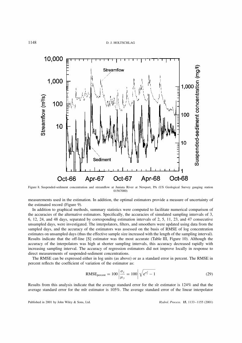
1148 D. J. HOLTSCHLAG
Figure 8. Suspended-sediment concentration and streamflow at Juniata River at Newport, PA (US Geological Survey gauging station01567000)
measurements used in the estimation. In addition, the optimal estimators provide a measure of uncertainty ofthe estimated record (Figure 9).
In addition to graphical methods, summary statistics were computed to facilitate numerical comparison ofthe accuracies of the alternative estimators. Specifically, the accuracies of simulated sampling intervals of 3,6, 12, 24, and 48 days, separated by corresponding estimation intervals of 2, 5, 11, 23, and 47 consecutiveunsampled days, were investigated. The interpolators, filters, and smoothers were updated using data from thesampled days, and the accuracy of the estimators was assessed on the basis of RMSE of log concentrationestimates on unsampled days (thus the effective sample size increased with the length of the sampling interval).Results indicate that the off-line [S] estimator was the most accurate (Table III, Figure 10). Although theaccuracy of the interpolators was high at shorter sampling intervals, this accuracy decreased rapidly withincreasing sampling interval. The accuracy of regression estimators did not improve locally in response todirect measurements of suspended-sediment concentrations.
The RMSE can be expressed either in log units (as above) or as a standard error in percent. The RMSE inpercent reflects the coefficient of variation of the estimator as:
RMSEpercent D 100
∣∣∣∣ �y%yD 100
∣∣∣∣√
e�2y � 1 �29
Results from this analysis indicate that the average standard error for the slr estimator is 124% and that theaverage standard error for the mlr estimator is 105%. The average standard error of the linear interpolator
Published in 2001 by John Wiley & Sons, Ltd. Hydrol. Process. 15, 1133–1155 (2001)

OPTIMAL ESTIMATION OF SUSPENDED-SEDIMENT CONCENTRATIONS 1149
Figure 9. Estimates and uncertainties of suspended-sediment concentrations at Juniata River at Newport, PA (US Geological Survey gaugingstation 01567000)
ranged from 48Ð4% for 3-day sampling intervals to 159% for 48-day sampling intervals. The average standarderror of the cubic-spline interpolator ranged from 50Ð6% for 3-day sampling intervals to 176% for 48-daysampling intervals. The average standard error for the on-line [F] estimator ranged from 52Ð7% for a 3-daysampling interval to 107% for a 48-day sampling interval. The average standard error for the off-line [S]estimator ranged from 39Ð9% for a 3-day sampling interval to 93Ð0% for a 48-day sampling interval. Thus,the off-line [S] estimator has the lowest standard error, especially at the shorter sampling intervals that areneeded to compute continuous records of suspended-sediment concentrations.
Possible sources of systematic variation in estimation errors among sites were investigated. In particular,off-line root mean square errors showed a slight tendency to decrease with increasing median discharges.Although the number of sites analysed is thought to be too small to provide conclusive results, the finding isconsistent with results by Phillips et al. (1999), who indicated that the accuracy and precision of the estimatorsthat they evaluated declined with a reduction in drainage area. No relation between model errors and sedimentcharacteristics was detected.
APPLICATION TO SEDIMENT COMPUTATION
Bias transformation adjustment
Exponentiation provides a simple transformation back to the original metric for estimates computed usinga log transformation. The mean of the exponentiated values, however, estimates the median of the original
Published in 2001 by John Wiley & Sons, Ltd. Hydrol. Process. 15, 1133–1155 (2001)

1150 D. J. HOLTSCHLAG
Table III. Estimation error characteristics at selected sites for specified sampling intervals (slr indicates simple linearregression, mlr indicates multiple linear regression, LinInt indicates linear interpolation, and CubSpl indicates cubio-spline
interpolation). The average root mean square error (mg/l) is given for days without measurements
Station name Estimator Simulated measurement interval (days)
3 6 12 24 48
Juniata River at Newport, PA slr 0Ð8868 0Ð8875 0Ð8877 0Ð8880 0Ð8875mlr 0Ð8231 0Ð8229 0Ð8240 0Ð8242 0Ð8235
LinInt 0Ð4372 0Ð6430 0Ð8287 0Ð9930 1Ð1791CubSpl 0Ð4488 0Ð6762 0Ð8768 1Ð0455 1Ð2450On-line 0Ð4495 0Ð5555 0Ð6600 0Ð7483 0Ð8063Off-line 0Ð3339 0Ð4339 0Ð5272 0Ð6297 0Ð7297
Sample size 9050 11 310 12 441 12 995 13 254Potomac River at Point of Rocks, MD slr 0Ð9388 0Ð9365 0Ð9380 0Ð9387 0Ð9387
mlr 0Ð7686 0Ð7653 0Ð7664 0Ð7674 0Ð7675LinInt 0Ð3878 0Ð5780 0Ð7669 0Ð9514 1Ð0680
CubSpl 0Ð3893 0Ð6068 0Ð8124 1Ð0193 1Ð1509On-line 0Ð4049 0Ð5044 0Ð5945 0Ð6859 0Ð7532Off-line 0Ð3054 0Ð3840 0Ð4746 0Ð5723 0Ð6869
Sample size 5896 7370 8107 8464 8648Rappahannock River at Remington, VA slr 0Ð9598 0Ð9567 0Ð9596 0Ð9584 0Ð9590
mlr 0Ð8812 0Ð8806 0Ð8834 0Ð8834 0Ð8845LinInt 0Ð6725 0Ð8823 1Ð0172 1Ð1663 1Ð2800
CubSpl 0Ð6989 0Ð9368 1Ð0705 1Ð2338 1Ð3480On-line 0Ð6018 0Ð6878 0Ð7793 0Ð8449 0Ð8795Off-line 0Ð4888 0Ð5791 0Ð6698 0Ð7756 0Ð8458
Sample size 6872 8590 9449 9867 10 058Yadkin River at Yadkin College, NC slr 0Ð7984 0Ð8007 0Ð8004 0Ð7983 0Ð7985
mlr 0Ð6541 0Ð6553 0Ð6540 0Ð6526 0Ð6525LinInt 0Ð4908 0Ð6929 0Ð8979 1Ð0140 1Ð1103
CubSpl 0Ð5086 0Ð7407 0Ð9604 1Ð0810 1Ð1814On-line 0Ð4406 0Ð5164 0Ð5766 0Ð6150 0Ð6360Off-line 0Ð3529 0Ð4353 0Ð5141 0Ð5712 0Ð6136
Sample size 9432 11 790 12 969 13 547 13 818Pee Dee River at Peedee, SC slr 0Ð4162 0Ð4174 0Ð4167 0Ð4167 0Ð4197
mlr 0Ð3678 0Ð3706 0Ð3694 0Ð3705 0Ð3715LinInt 0Ð3400 0Ð4133 0Ð4440 0Ð4830 0Ð5024
CubSpl 0Ð3583 0Ð4388 0Ð4688 0Ð5098 0Ð5544On-line 0Ð3176 0Ð3434 0Ð3627 0Ð3706 0Ð3721Off-line 0Ð2834 0Ð3189 0Ð3489 0Ð3628 0Ð3673
Sample size 976 1220 1342 1403 1410Edisto River near Givhans, SC slr 0Ð5580 0Ð5557 0Ð5555 0Ð5536 0Ð5529
mlr 0Ð5235 0Ð5220 0Ð5212 0Ð5186 0Ð5191LinInt 0Ð4272 0Ð4526 0Ð4622 0Ð4918 0Ð5215
CubSpl 0Ð4604 0Ð4794 0Ð4893 0Ð5277 0Ð5407On-line 0Ð4543 0Ð4822 0Ð5038 0Ð5109 0Ð5160Off-line 0Ð4129 0Ð4481 0Ð4849 0Ð5009 0Ð5124
Sample size 1342 1675 1837 1909 1927Colorado River near Cisco, UT slr 1Ð2530 1Ð2580 1Ð2573 1Ð2584 1Ð2560
mlr 1Ð1054 1Ð1097 1Ð1083 1Ð1097 1Ð1068LinInt 0Ð4056 0Ð5936 0Ð7888 0Ð9177 1Ð0585
CubSpl 0Ð4226 0Ð6222 0Ð8369 0Ð9609 1Ð1271On-line 0Ð5147 0Ð6913 0Ð8617 1Ð0281 1Ð1851Off-line 0Ð3704 0Ð5062 0Ð6617 0Ð7788 0Ð9226
Sample size 3996 4995 5489 5727 5828(continued on next page)
Published in 2001 by John Wiley & Sons, Ltd. Hydrol. Process. 15, 1133–1155 (2001)

OPTIMAL ESTIMATION OF SUSPENDED-SEDIMENT CONCENTRATIONS 1151
Table III. (continued )
Station name Estimator Simulated measurement interval (days)
3 6 12 24 48
San Juan River near Bluff, UT slr 0Ð9616 0Ð9570 0Ð9597 0Ð9588 0Ð9590mlr 0Ð8823 0Ð8776 0Ð8802 0Ð8797 0Ð8790
LinInt 0Ð3148 0Ð4306 0Ð5876 0Ð7411 0Ð8683CubSpl 0Ð3183 0Ð4506 0Ð6245 0Ð7836 0Ð9230On-line 0Ð4383 0Ð5384 0Ð6557 0Ð7403 0Ð8449Off-line 0Ð3079 0Ð4020 0Ð5340 0Ð6460 0Ð7550
Sample size 3922 4900 5390 5635 5734Green River at Green River, UT slr 0Ð9730 0Ð9757 0Ð9770 0Ð9775 0Ð9775
mlr 0Ð9536 0Ð9563 0Ð9552 0Ð9562 0Ð9562LinInt 0Ð3500 0Ð5145 0Ð7679 0Ð9256 1Ð1197CubSpl 0Ð3619 0Ð5357 0Ð8225 0Ð9588 1Ð1775On-line 0Ð4164 0Ð5627 0Ð6966 0Ð8291 0Ð9546Off-line 0Ð3041 0Ð4018 0Ð5354 0Ð6558 0Ð8054
Sample size 1694 2115 2321 2415 2444Paria River at Lees Ferry, AZ slr 1Ð9171 1Ð9195 1Ð9209 1Ð9191 1Ð9187
mlr 1Ð666 1Ð6712 1Ð6731 1Ð6729 1Ð6722LinInt 0Ð7965 1Ð1408 1Ð5457 2Ð0766 2Ð5059CubSpl 0Ð8090 1Ð1846 1Ð6546 2Ð2199 2Ð6274On-line 0Ð9152 1Ð2240 1Ð4594 1Ð6589 1Ð8124Off-line 0Ð6450 0Ð8960 1Ð1448 1Ð4237 1Ð6553
Sample size 6816 8520 9372 9798 10 011
Figure 10. Average root mean square error of selected estimators for specified sampling intervals
Published in 2001 by John Wiley & Sons, Ltd. Hydrol. Process. 15, 1133–1155 (2001)

1152 D. J. HOLTSCHLAG
population rather than the mean. For log-normally distributed populations, the median is less than the mean.Thus, the mean of the exponentiated estimates generally is thought to underestimate the mean suspended-sediment concentration. In contradiction, Walling and Webb (1988) show that exponentiated estimates thatare adjusted for this possible bias are significantly less accurate and less precise than estimates that arenot adjusted, based on load calculations derived from rating curves. If adjustment is desired, however,the ‘smearing’ approach (Helsel and Hirsch, 1992) provides a nonparametric bias correction factor (BCF)applicable to optimal estimates of suspended-sediment concentrations. For off-line [S] estimates, the BCF iscomputed as the mean of the exponentiated residuals:
BCF Dn∑iD1
exp[yi � y[S]i]
n�30
The residuals, which may follow any distribution, are only assumed to be independent and homoscedastic. Forapplication, the BCF is multiplied by the exponentiation smoothed estimates to compute the mean suspended-sediment concentrations.
Unit value computation
Because of the nonlinear relation (in arithmetic space rather than log space) between streamflowand suspended-sediment concentrations and occasionally large daily ranges in streamflow, daily averagesuspended-sediment concentrations are typically computed based on unit (less than daily) values rather thandaily average streamflow values. It is anticipated that future applications of the estimators will be based ona development from unit values and direct measurement data. If the unit value data are difficult to obtain,however, the dynamics determined from analysis of daily values data can be applied to shorter intervals, withadjustments described in the following section.
The state-space model contains static components, associated with the effects of streamflow and seasonality,and dynamic components, associated with the error characteristics. The explanatory variable associated withthe static effect of changes in streamflow rate, uk,4, on sediment concentrations must be recomputed for thesize of the unit time step. The parameters associated with the static effects, however, may still be applicable.In contrast, values of � and Qk characterize the dynamic error in sediment concentrations at a time step of 1day. The following section describes how to adjust daily estimates of � and Qk for computation at unit timeintervals.
The discrete time (difference) equation for the state equation was developed with a time index k having aconstant size k equal to 1 day and was expressed as:
�k D �·�k�1 C wk�1 �31
To convert this equation for use with an alternate size of time step, Equation (31) is first converted to acontinuous time (differential) equation of the form:
P�t D F�t C wt �32
which indicates that the rate of change in the state variable is proportional to its present state. Thisproportionality factor is simply computed as:
F D log[�] �33
For application at a new sampling interval k1, equal to say 1/24 day, and indexed by k1, � and the stateequation are revised as:
�1 D eF·k1
�k1 D �1·�k1�1 C wk1�1
�34
Published in 2001 by John Wiley & Sons, Ltd. Hydrol. Process. 15, 1133–1155 (2001)

OPTIMAL ESTIMATION OF SUSPENDED-SEDIMENT CONCENTRATIONS 1153
with a result that �1 > � for unit time intervals shorter than 1 day. Converting Qk to an alternate time stepis an extension of this procedure. First, the discrete process variance determined at k D 1 is related to thecontinuous process variance Q) as:
Qk D eFk{∫ k
0e�F)Q) e�FT
) d)}
eFTk �35
(Grewal and Andrews, 1993). Solving Equation (35) for Q) results in:
Q) D 2F·Qk
�1 C e2F·k �36
The corresponding discrete time covariance for discrete time interval k1 can then be computed as:
Qk1 D Q) e2Fk1
[ �1
2 e2F·k1FC 1
2F
]�37
Finally, the magnitude of the measurement covariance, Rk , may be decreased because the direct (instantaneous)measurements of suspended-sediment concentrations contain smaller time-sampling errors than those presentin daily average values. Methods described by Burkham (1985) may be helpful in revising the estimate ofRk . Once the values of �, Qk , Rk , and uk,4 are revised, the previously developed Kalman filter and smootherequations may be applied.
Implication for sampling design
The analyses described in this paper were based on long-term suspended-sediment concentration records,which had an average length of 6901 daily observations without missing values. Although application to shorterrecord length with missing data was not assessed, the following observations may provide a useful preliminaryguide to these types of situations. The SAS AUTOREG procedure was used to estimate model parameters.The documentation for this procedure suggests that the maximum likelihood estimation method be used ifmissing values are ‘plentiful’ (SAS Institute, 1988, p. 177). Although ‘plentiful’ is not explicitly defined,it is assumed to be related to both the length of record and the percentage of missing values. Should datacharacteristics limit the number of parameters that can be estimated or found statistically significant by use ofthis method, a simpler model structure might be used initially, perhaps eliminating terms for the streamflowderivative or seasonal component. Additionally, systematic sampling at a fixed interval limits informationavailable on the covariance structure, which is used in filtering and smoothing operations, to multiples ofthe fixed interval. Then, covariance information at shorter intervals must be projected from multiples of thesampling interval. For example, if systematic sampling occurs at 15-day intervals, the covariance structureis empirically defined only for 15, 30, 45-day intervals and so on, and must be extrapolated to 1-day orunit intervals for record computation. This type of extrapolation introduces additional uncertainty in theestimation process, and might be avoided by varying the sampling interval while maintaining the same totalnumber of samples. Additional analyses are needed to more fully investigate the implications for samplingdesign.
SUMMARY
This paper develops optimal estimators for on-line and off-line computation of suspended-sediment con-centrations in streams and compares the accuracies of the optimal estimators with results produced bytime-averaging interpolators and flow-weighting regression estimators. The analysis uses long-term daily-mean suspended-sediment concentration and streamflow data from 10 sites within the United States to compareaccuracies of the estimators. A log transformation was applied to both suspended-sediment concentration and
Published in 2001 by John Wiley & Sons, Ltd. Hydrol. Process. 15, 1133–1155 (2001)

1154 D. J. HOLTSCHLAG
streamflow values prior to development of the estimates. Standard techniques are described for removingthe possible bias in estimates of the mean computed form exponentiated values of sediment concentra-tion computed in log units and for approximating instantaneous or unit dynamics on the basis of dailysamples.
The optimal estimators are based on a Kalman filter and an associated smoother to produce the on-lineand off-line estimates, respectively. The optimal estimators included site-specific parameters, which wereestimated by generalized least squares, to account for influences associated with ancillary variables, includingstreamflow and annual seasonality, on suspended-sediment concentrations. In addition, the optimal estimatorsaccount for autoregressive error components and uncertainties in the accuracy of direct measurements incomputing continuous records of suspended-sediment concentrations. Results were compared with estimatesproduced by both linear and cubic-spline interpolators, which do not account for ancillary variables, andwith simple and multiple-regression estimators, which do not locally account for direct measurements ofsuspended-sediment concentration.
The average standard error of simple and multiple regression estimates was 124 and 105%, respectively.The accuracies of interpolators, and on-line and off-line estimators are related to measurement frequency,and were compared at simulated measurement intervals of 3, 6, 12, 24, and 48 days. The average standarderror of the linear interpolator ranged from 48Ð4% for 3-day sampling intervals to 159% for 48-day samplingintervals. The average standard error of the cubic-spline interpolator ranged from 50Ð6% for 3-day samplingintervals to 176% for 48-day sampling intervals. The average standard error for the on-line estimator rangedfrom 52Ð7% for a 3-day sampling interval to 107% for a 48-day sampling interval. The average standard errorfor the off-line estimator ranged from 39Ð9% for a 3-day sampling interval to 93Ð0% for a 48-day samplinginterval. Thus, the off-line estimator had the lowest standard error, especially at the shorter sampling intervalsthat are needed to compute continuous records of suspended-sediment concentrations.
The use of the optimal estimators rather than interpolators or regression estimators will improve the accuracyand quantify the uncertainty of records computed on the basis of suspended-sediment concentrations measuredat intervals less than 48 days. Although in this paper, parameters for the estimators were developed on thebasis of daily values data, it is anticipated that in typical applications the estimators will be developed on thebasis of unit-value data and direct measurement information.
REFERENCES
Bukaveckas PA, Likens GE, Winter TC, Buso DC. 1998. A comparison of methods for deriving solute flux rates using long-term data fromstreams in the Mirror Lake watershed. Water, Air, and Soil Pollution 105: 277–293.
Burkham DE. 1985. An approach for appraising the accuracy of suspended-sediment data. US Geological Survey Professional Paper 1333:18.
Ferguson RI. 1986. River loads underestimated by rating curves. Water Resources Research 22(1): 74–76.Gelb A (ed.). 1974. Applied Optimal Estimation. MIT Press: Cambridge, MA; 374.Glysson GD. 1987. Sediment-transport curves. US Geological Survey Open-File Report 87–218: 47.Grewal MS, Andrews AP. 1993. Kalman Filtering—Theory and Practice. Prentice Hall Information and System Science Series: Englewood
Cliffs, NJ; 38.Guy HP. 1970. Fluvial sediment concepts. US Government Printing Office: Washington, DC; US Geological Survey Techniques of Water-
Resources Investigations, Vol. 3, Chap. C1. 55.Guy HP, Norman VW. 1973. Field methods for measurement of fluvial sediment. US Government Printing Office: Washington, DC; US
Geological Survey Techniques of Water-Resource Investigations, Vol. 3, Chap. C2. 59.Helsel DR, Hirsch RM. 1992. Statistical Methods in Water Resources. Studies in Environmental Science Vol. 49. Elsevier: New York; 522.Koltun GF, Gray JR, McElhone TJ. 1994. User’s manual for SEDCALC, a computer program for computation of suspended-sediment
discharge. US Geological Survey Open-File Report 94–459: 46.Phillips JM, Webb BW, Walling DE, Leeks GJL. 1999. Estimating the suspended sediment loads of rivers in the LOIS study area using
infrequent samples. Hydrological Processes 13(7): 1035–1050.Porterfield G. 1972. Computation of fluvial-sediment discharge. US Government Printing Office: Washington, DC; US Geological Survey
Techniques of Water-Resources Investigations, Vol. 3, Chap. C3. 66.Richards RR, Holloway J. 1987. Monte Carlo studies of sampling strategies for estimating tributary loads. Water Resources Research 23(10):
1939–1948.SAS Institute. 1988. SAS/ETS User’s Guide, Vers. 6, 1st ed. SAS Institute: Cary NC; 560 pp.
Published in 2001 by John Wiley & Sons, Ltd. Hydrol. Process. 15, 1133–1155 (2001)

OPTIMAL ESTIMATION OF SUSPENDED-SEDIMENT CONCENTRATIONS 1155
Siouris GM. 1996. Optimal Control and Estimation Theory . Wiley: New York; 407.Walling DE, Webb BW. 1988. The reliability of rating curve estimates of suspended sediment yield; some further comments. In Sediment
Budgets , Bordas MP, Walling DE (eds). IAHS Publication No. 174; 350.Yang CT. 1996. Sediment Transport—Theory and Practice. McGraw-Hill: New York; 396.
Published in 2001 by John Wiley & Sons, Ltd. Hydrol. Process. 15, 1133–1155 (2001)