Charles University in Prague

Faculty of Mathematics and Physics

BACHELOR THESIS

Tomas Musil

Optical Game Position Recognition inthe Board Game of Go

Department of Applied Mathematics

Supervisor of the bachelor thesis: Mgr. Petr Baudis

Study programme: Computer Science

Specialization: General Computer Science

Prague 2014

I would like to thank Mgr. Petr Baudis for his supervision, patience and valuableadvice. I would also like to thank my parents for their support during my studies.

I declare that I carried out this bachelor thesis independently, and only with thecited sources, literature and other professional sources.

I understand that my work relates to the rights and obligations under the ActNo. 121/2000 Coll., the Copyright Act, as amended, in particular the fact thatthe Charles University in Prague has the right to conclude a license agreementon the use of this work as a school work pursuant to Section 60 paragraph 1 ofthe Copyright Act.

In Prague 30. 7. 2014 signature of the author

Nazev prace: Rozpoznavanı pozic deskove hry go z fotografiı

Autor: Tomas Musil

Katedra: Katedra aplikovane matematiky

Vedoucı bakalarske prace: Mgr. Petr Baudis, Katedra aplikovane matematiky

Abstrakt: Pri profesionalnıch a turnajovych partiıch ve hre go byva obvykleporizovan jejich zapis. I neformalnı partie muze byt uzitecne si zaznamenat propotreby pozdejsı analyzy a studia. Porizovanı zaznamu vsak hrace rusı od hrya snadno se pri nem udela chyba. Videozaznam nebo soubor fotografiı postradaflexibilitu abstraktnı notace. V teto praci popisujeme mozne postupy pri auto-maticke extrakci hernıch pozic z fotografiı. Navrhujeme vlastnı algoritmus za-lozeny na Houghove transformaci a metode RANSAC. Soucastı prace je imple-mentace programu, ktery tento algoritmus vyuzıva k tomu, aby umoznil hracumpartii snadno a spolehlive zaznamenat.

Klıcova slova: pocıtacove videnı, hra go

Title: Optical Game Position Recognition in the Board Game of Go

Author: Tomas Musil

Department: Department of Applied Mathematics

Supervisor: Mgr. Petr Baudis, Department of Applied Mathematics

Abstract: It is customary to keep a written game record of professional or high-rank amateur tournament games of Go. Even informal games are worth recordingfor subsequent analysis. Writing the game record by hand distracts the playerfrom the game and it is not very reliable. Video or photographic record lacksthe flexibility of abstract notation. In this thesis we discuss several ways ofautomatically extracting Go game records from photographs. We propose ourown method based on Hough transform and RANSAC paradigm. We implementa reliable and easy to use system that allows players to take a game recordeffortlessly.

Keywords: computer vision, game of go, baduk

Contents

Introduction 2

1 Theory and algorithms 41.1 Perspective . . . . . . . . . . . . . . . . . . . . . . . . . . . . . . 41.2 Color spaces . . . . . . . . . . . . . . . . . . . . . . . . . . . . . . 41.3 Hough transform . . . . . . . . . . . . . . . . . . . . . . . . . . . 51.4 RANSAC . . . . . . . . . . . . . . . . . . . . . . . . . . . . . . . 6

2 Analysis of the problem 82.1 Overview . . . . . . . . . . . . . . . . . . . . . . . . . . . . . . . . 82.2 Finding the grid . . . . . . . . . . . . . . . . . . . . . . . . . . . . 82.3 Finding the stones . . . . . . . . . . . . . . . . . . . . . . . . . . 102.4 Sequences of images . . . . . . . . . . . . . . . . . . . . . . . . . . 112.5 Video . . . . . . . . . . . . . . . . . . . . . . . . . . . . . . . . . 12

3 Related works 133.1 Academic work . . . . . . . . . . . . . . . . . . . . . . . . . . . . 133.2 Available software . . . . . . . . . . . . . . . . . . . . . . . . . . . 14

4 Game position recognition 174.1 Finding the grid . . . . . . . . . . . . . . . . . . . . . . . . . . . . 174.2 Finding the stones . . . . . . . . . . . . . . . . . . . . . . . . . . 184.3 Video . . . . . . . . . . . . . . . . . . . . . . . . . . . . . . . . . 18

5 Implementation 245.1 Imago . . . . . . . . . . . . . . . . . . . . . . . . . . . . . . . . . 245.2 Technical documentation . . . . . . . . . . . . . . . . . . . . . . . 24

6 Evaluation 276.1 Dataset . . . . . . . . . . . . . . . . . . . . . . . . . . . . . . . . 276.2 Experimental results . . . . . . . . . . . . . . . . . . . . . . . . . 27

Conclusion 29Future works . . . . . . . . . . . . . . . . . . . . . . . . . . . . . . . . 29

Bibliography 30

A User documentation 32

B The attached CD 33

1

Introduction

The game of Go

The game of Go is an ancient board game, originating in China. It was firstmentioned in Chinese writings from Honan dating from about 625 B. C. (Bell,1979).

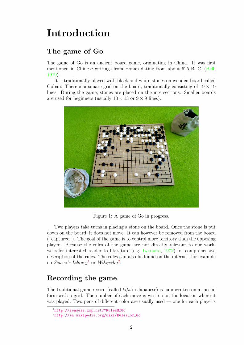
It is traditionally played with black and white stones on wooden board calledGoban. There is a square grid on the board, traditionally consisting of 19 × 19lines. During the game, stones are placed on the intersections. Smaller boardsare used for beginners (usually 13× 13 or 9× 9 lines).

Figure 1: A game of Go in progress.

Two players take turns in placing a stone on the board. Once the stone is putdown on the board, it does not move. It can however be removed from the board(“captured”). The goal of the game is to control more territory than the opposingplayer. Because the rules of the game are not directly relevant to our work,we refer interested reader to literature (e.g. Iwamoto, 1972) for comprehensivedescription of the rules. The rules can also be found on the internet, for exampleon Sensei’s Library1 or Wikipedia2.

Recording the game

The traditional game record (called kifu in Japanese) is handwritten on a specialform with a grid. The number of each move is written on the location where itwas played. Two pens of different color are usually used — one for each player’s

1http://senseis.xmp.net/?RulesOfGo2http://en.wikipedia.org/wiki/Rules_of_Go

2

moves — to make the game record easier to read. Any mistakes in a handwrittenrecord are hard to correct.

Today, computers, tablets or smartphones can be used to record the game.This facilitates the recording, because mistakes are easily corrected and the result-ing game record can be displayed conveniently. But it still distracts the recordingplayer from the game.

Outline of this thesis

In this thesis, we examine possibilities of automatic optical game position recog-nition in Go. We implement a system that enables players to record their gameeasily, with just a (web)camera and a computer. The recording is fully automaticand does not distract the player from the game. It is reliable and the resultinggame record can be easily displayed and edited in any Go editing program.

In Chapter 1 we introduce basic notions of perspective geometry, color theoryand we describe algorithms that are used later on. In Chapter 2 we give a detailedoverview of the problem of optical recognition of Go positions. In Chapter 3 wesurvey related academic works and currently available Go recording software. Wedescribe our method of game position recognition in Chapter 4 and the applica-tion based on it in Chapter 5. We evaluate performance of our application inChapter 6.

3

1. Theory and algorithms

In this chapter we explain some basic theoretic notions and algorithms that willbe used in following chapters.

1.1 Perspective

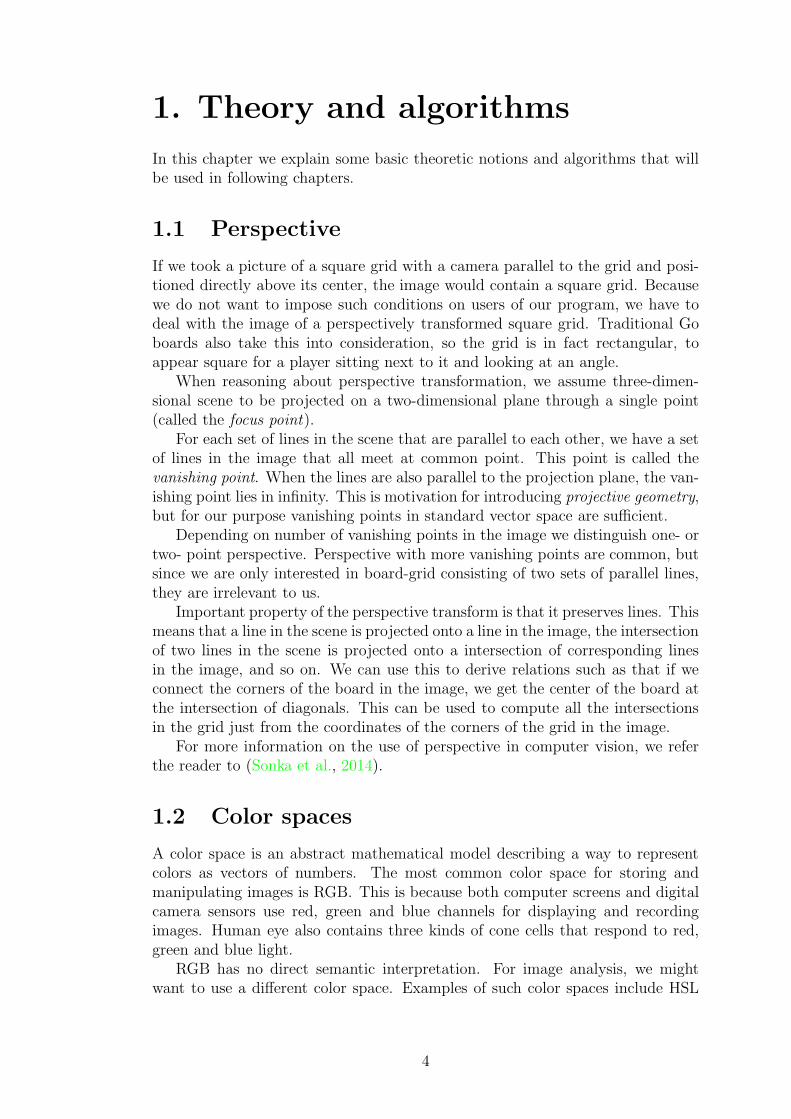
If we took a picture of a square grid with a camera parallel to the grid and posi-tioned directly above its center, the image would contain a square grid. Becausewe do not want to impose such conditions on users of our program, we have todeal with the image of a perspectively transformed square grid. Traditional Goboards also take this into consideration, so the grid is in fact rectangular, toappear square for a player sitting next to it and looking at an angle.

When reasoning about perspective transformation, we assume three-dimen-sional scene to be projected on a two-dimensional plane through a single point(called the focus point).

For each set of lines in the scene that are parallel to each other, we have a setof lines in the image that all meet at common point. This point is called thevanishing point. When the lines are also parallel to the projection plane, the van-ishing point lies in infinity. This is motivation for introducing projective geometry,but for our purpose vanishing points in standard vector space are sufficient.

Depending on number of vanishing points in the image we distinguish one- ortwo- point perspective. Perspective with more vanishing points are common, butsince we are only interested in board-grid consisting of two sets of parallel lines,they are irrelevant to us.

Important property of the perspective transform is that it preserves lines. Thismeans that a line in the scene is projected onto a line in the image, the intersectionof two lines in the scene is projected onto a intersection of corresponding linesin the image, and so on. We can use this to derive relations such as that if weconnect the corners of the board in the image, we get the center of the board atthe intersection of diagonals. This can be used to compute all the intersectionsin the grid just from the coordinates of the corners of the grid in the image.

For more information on the use of perspective in computer vision, we referthe reader to (Sonka et al., 2014).

1.2 Color spaces

A color space is an abstract mathematical model describing a way to representcolors as vectors of numbers. The most common color space for storing andmanipulating images is RGB. This is because both computer screens and digitalcamera sensors use red, green and blue channels for displaying and recordingimages. Human eye also contains three kinds of cone cells that respond to red,green and blue light.

RGB has no direct semantic interpretation. For image analysis, we mightwant to use a different color space. Examples of such color spaces include HSL

4

and HSV (Joblove and Greenberg, 1978). These spaces consist of hue, saturation,and lightness/value, which are easier to interpret than RGB values.

To obtain a gray-scale image from a polychromatic one, we use luminance. Itcomes from the YUV color space and its variants, which are mostly used in videoencoding. The luminance is defined as Y = 0.2126R + 0.7152G+ 0.0722B. Thisreflects the fact that green light contributes the most to human visual perceptionof intensity, and blue light the least. Digital cameras usually have better resolu-tion in the green channel, so it makes sense to give the biggest weight to green inimage analysis as well.

1.3 Hough transform

The Hough transform for lines was introduced by Duda and Hart (1972), buildingon a previous work by Hough (1962).

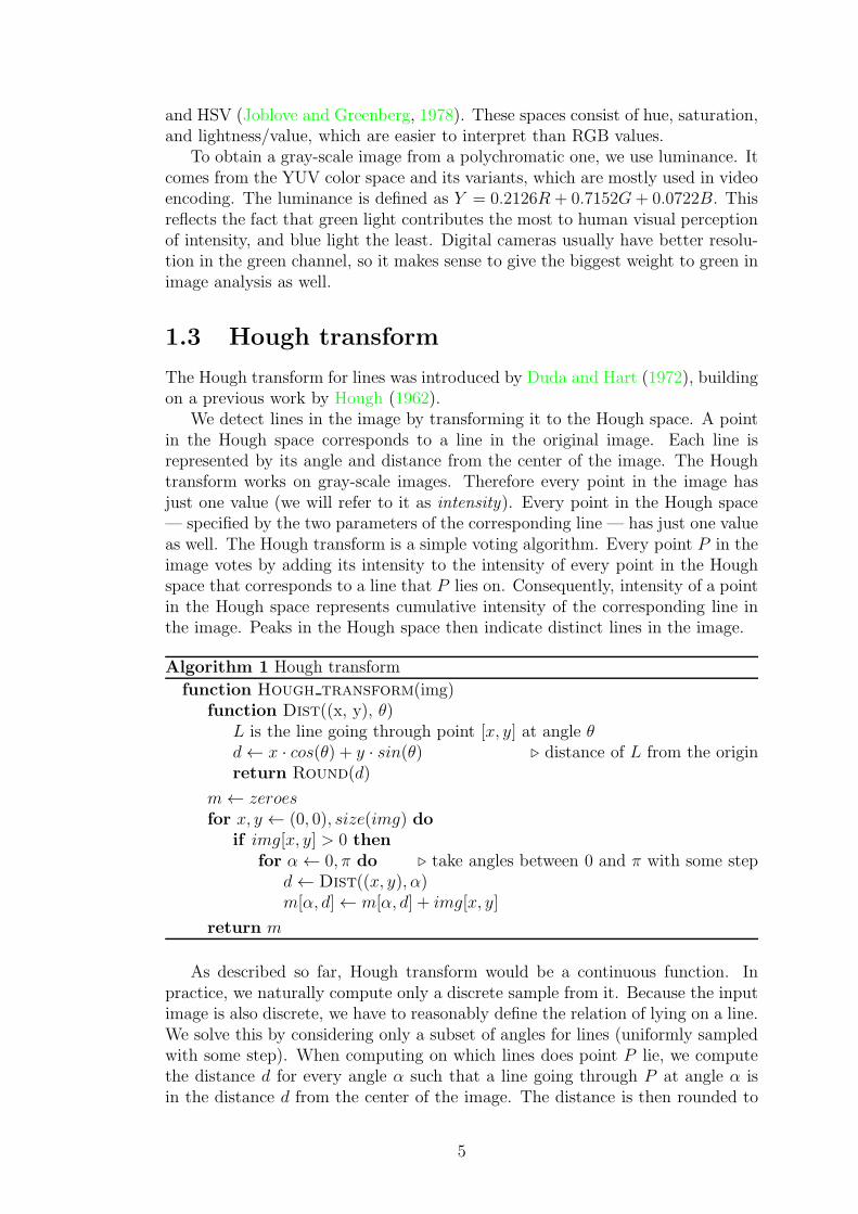
We detect lines in the image by transforming it to the Hough space. A pointin the Hough space corresponds to a line in the original image. Each line isrepresented by its angle and distance from the center of the image. The Houghtransform works on gray-scale images. Therefore every point in the image hasjust one value (we will refer to it as intensity). Every point in the Hough space— specified by the two parameters of the corresponding line — has just one valueas well. The Hough transform is a simple voting algorithm. Every point P in theimage votes by adding its intensity to the intensity of every point in the Houghspace that corresponds to a line that P lies on. Consequently, intensity of a pointin the Hough space represents cumulative intensity of the corresponding line inthe image. Peaks in the Hough space then indicate distinct lines in the image.

Algorithm 1 Hough transform

function Hough transform(img)function Dist((x, y), θ)

L is the line going through point [x, y] at angle θ

d← x · cos(θ) + y · sin(θ) ⊲ distance of L from the originreturn Round(d)

m← zeroes

for x, y ← (0, 0), size(img) doif img[x, y] > 0 then

for α← 0, π do ⊲ take angles between 0 and π with some stepd← Dist((x, y), α)m[α, d]← m[α, d] + img[x, y]

return m

As described so far, Hough transform would be a continuous function. Inpractice, we naturally compute only a discrete sample from it. Because the inputimage is also discrete, we have to reasonably define the relation of lying on a line.We solve this by considering only a subset of angles for lines (uniformly sampledwith some step). When computing on which lines does point P lie, we computethe distance d for every angle α such that a line going through P at angle α isin the distance d from the center of the image. The distance is then rounded to

5

the nearest point in the discrete Hough space. We use angles from 0 to π andnegative distance, so all parallel lines have the same angle but different distance.

For the pseudocode, see Algorithm 1. See figures 4.2 and 4.3 for an exampleof an image and its Hough transform.

O’Gorman and Clowes (1976) improved the Hough transform by using localgradient to reduce the number of useless votes and computation time. The Houghtransform was further generalized to detect arbitrary shapes by Ballard (1981).

1.4 RANSAC

The RANSAC (RANdom Sample And Consensus) algorithm was first introducedby Fischler and Bolles (1981). It is a stochastic method for estimation of theparameters of a model from data contaminated by large amount of outliers.

Figure 1.1: RANSAC estimate of a linear model. Dataset consists of all the dots,red line shows the model estimated by the least squares method, blue line showsthe Theil-Sen estimate, green line shows the model estimated by RANSAC (withconsensus set consisting of green dots).

We will illustrate the RANSAC process with an example of a linear model.Suppose we have some data generated from a linear model with Gaussian noise(e.g. green dots in Fig. 1.1). We would like to estimate the parameters of themodel. In this case, we can just use the least squares method (the green line inFig. 1.1) to estimate the parameters of the model.

Now we take the data generated from the same model, but this time withoutliers (blue dots in Fig. 1.1). The outliers are distributed arbitrarily, thereforewe cannot expect their deviations from the model to cancel out. As you can see,there can be quite a lot of outliers, but the line can still be distinguished. Thistime, the least squares (red line in Fig. 1.1) are quite off. Theil-Sen estimate

6

(Sen, 1968) is better, but still not good enough (blue line in Fig. 1.1). This iswhere RANSAC helps.

Algorithm 2 RANSAC algorithm

procedure RANSAC(data, distance, threshold, max iter)best← {}i← 0while |best| < threshold and i < max iter do

consensus← random sample(data)c← 0while c < |consensus| do

c← |consensus|model ← estimate(consensus)consensus← filter(model, data, distance)

if |best| < |consensus| thenbest← consensus

i← i+ 1

return best

In each RANSAC iteration we randomly select exactly enough datapointsto determine the parameters of the model (2 datapoints in the two-dimensionallinear case). Then we check all the datapoints against this model. We createa so called consensus set, consisting of datapoints that are closer than d to themodel (d is a parameter). We assume that the consensus set consist of inliers,therefore we can use e.g. least squares method to create a new estimate of theparameters based on the consensus set. We create a new consensus set for thenew model. We continue with re-estimating the model (based on the consensusset) and recomputing the consensus set (based on the model) until the consensusset stops growing. For common models and estimators, this part can be regardedas an instance of EM algorithm.

We repeat the whole cycle of randomly sampling the data and improvingthe model, until we find a suitable solution or reach a predetermined number ofiterations. In Figure 1.1 we end with consensus set consisting of green dots andthe corresponding model is visualized by the green line.

If we have an apriori estimate of the ratio of outlier and inliers, Fischler andBolles (1981) give an estimate on number of iterations needed to achieve selectedprobability of finding the correct consensus set.

There are many variations to the RANSAC algorithm. One important mod-ification is MSAC (Torr and Zisserman, 1998), where the inliers are scored bytheir fitness to the model and outliers are given constant weight. This does notpresent any computational overhead, but it can lead to better results. Anothermodification is MLESAC (Torr and Zisserman, 2000), where the consensus set isscored by its likelihood, instead of its cardinality.

For more information on RANSAC we recommend an excellent guide writtenby Zuliani (2014).

7

2. Analysis of the problem

In this chapter we analyze various potential solutions to the problem of opticalposition recognition in Go. In Section 2.1 we provide an overview of the problemand discuss the assumptions we make about the input. In sections 2.2 through2.5 we examine individual stages of the game position recognition.

2.1 Overview

There are many features that we can use to find the board in the image. Humanbrains probably use many of them simultaneously. We could for example clusterthe pixels of the image by their distance in color space. This would work inmany cases, except for a fairly common situation of wooden board on a woodentable. The most reliable system would combine all of these features in order towork in any conceivable conditions. Unfortunately, because we are working withimage data, the computations for such a system would take intolerable amountof resources. We need to carefully select what features we use in order to balancereliability with speed, if we want to build a system that is effectively usable.

This differs from general pattern recognition tasks in that we can exploit thegeometric properties of the grid. In following paragraphs, we present variouspossibilities to do so.

2.2 Finding the grid

First step of the position recognition is locating the grid. We could try to locatethe board and restrict the search for the grid to the appropriate area of the image,but this not necessary.

To simplify the analysis, we assume that there are no stones on the board.We deal with stones in the last paragraph of this section.

Detecting the edges To lower the amount of noise in subsequent stages ofrecognition, we might detect edges in the image and use them instead of theoriginal image. We assume that the grid consists of dark lines on light background,therefore we can use a simple filter to detect edges. The filter approximates theLaplacian of the image, by computing a convolution sum with the following mask(so called Laplace operator):

L =

1 1 11 −8 11 1 1

There are many other methods for edge detection, see (Sonka et al., 2014) fora survey.

Finding the lines We find the edges. Then we use the Hough transform.Peaks in the Hough space correspond to strong lines in the image. Now we needto find the lines that belong to the grid.

8

Points representing lines that are parallel in the scene lie almost on a line inHough space. They actually lie on a sinusoid, as lines that are parallel in the sceneintersect at a vanishing point in the image plane and each point in the image isprojected on a sinusoid in Hough space. But if we assume that we see the boardunder reasonable angle, then the vanishing point is far away from the center ofthe image, therefore the sinusoid formed by the vanishing point in the Houghspace has a large amplitude (x or y are large in d = x · sin(θ) + y · cos(θ)). Weare interested only in values relatively close to zero, because lines correspondingto larger values are out of the image. And the part of the sinusoid that is nearthe zero can be safely approximated by linear function.

Therefore we can easily find the two sets of lines that are parallel in the sceneand form the grid, as they lie on two lines in Hough space. Some lines might bemissing and we will usually find some extra ones (e.g. edges of the board).

Perspective We can use properties of perspective to try to find the grid an-alytically. If we assume two-point projection, we can find vanishing points forboth sets of lines. They determine the horizon line. Intersections of grid-lineswith any line parallel to the horizon are evenly spaced on the horizon-parallelline. The Fourier transform can be used to find the strongest frequency, whichcorresponds to the spacing of the grid-lines. Once we have the spacing, its easyto select a grid that maximizes the likelihood of observed lines.

There are also images, that are closer to one point perspective. Those can beanalyzed similarly. For images with no point perspective (camera parallel to theboard) the analysis is even simpler.

Finding the grid by minimization The problem of locating the grid in theimage can be modeled as a minimization problem. To do so, we need to choosea method for generating candidates for the grid and a function to minimize.

Selecting the parameters is important part of the minimization formulation.The more information we can get from the analysis of the image (e.g. angles of thelines from the Hough transform), the less parameters we need. The less param-eters we use, the faster the computation. On the other hand, if the informationused to restrict the search space was inaccurate or even wrong, it prevents usfrom reaching the correct solution.

If we parametrize on positions of the corners, we have eighth parameters. If weconsider the position of the camera relative to the board, we have six parameters.We can estimate the angles of lines from the Hough transform and take only theirdistance from the center of the image as parameters (then we have four).

Next we need to choose a cost function. The cost function can compare thecandidate to the edges detected in the image, to the lines detected from the edgesor their intersections. The first approach seems to be the most reliable, but it isalso the most computationally demanding.

In any configuration, this is quite costly to compute. The problem is in itsessence non-convex with many local minima (e.g. the position with grid shift-ed by one line). Therefore we cannot use gradient descent and must resort tostochastic optimization method such as Particle Swarm Optimization (Kennedyand Eberhart, 1995) or Cuckoo Search (Yang and Deb, 2009).

9

Selecting the lines We can try to build the grid from the lines that we foundby the Hough transform. We must somehow deal with some extra lines andsome grid-lines missing. Exploring all possible combinations is computationallyexpensive. But we can employ a RANSAC-inspired approach: select two lines ineach direction at random, try various configurations of the grid (each of selectedlines being interpreted as first, second, third, . . . , line of the grid), repeat thisa few times, pick the best candidate. The score of the candidates can be any ofthe functions mentioned in previous paragraph.

Finding the center Another method is based on finding the center and di-agonals of the grid first. Once we have the center and angles from the Houghtransform, the grid is determined by just two corners. We can further narrow thisdown by finding the diagonals of the grid first. Because diagonals go through thelargest number of intersections (except for the lines that we already have), theycan be found with RANSAC.

Polygons Instead of finding lines in the image, we can try to detect polygons.We assume that most of the polygons in the image will be on the board and theywill all be roughly the same size in the perspective projection. Therefore we canfind the median distance and discard all polygons that deviate from it too much.Then we take the convex hull of the remaining polygons and we should end upwith the grid.

Corners and intersections There are extensions to the Hough transform forfinding the corners and intersections of lines (Barrett and Petersen, 2001). Thiscould be used to find the intersections. The result would not contain false inter-sections, that we get when simply computing intersections of lines found by theHough transform.

Stones on the board Detecting lines with Hough transform works even withstones on the board. With too many stones on the board, the lines get obscuredand harder to detect. Rules of Go allow the board to be almost completely filledwith stones. In that case we would need to detect stones instead of lines. Houghtransform for circles could be used for that. But the board is highly unlikely toget completely covered in a real game. In Figure 2.1 we see two finished gameswith lines detected by the Hough transform. Some lines are missing, but thereare clearly enough lines to find the grid.

2.3 Finding the stones

When detecting stones, we can ignore the perspective transformation. Under anyreasonable angle, Go stones are projected as roughly circular shape, either blackor white.

Based on color If we know the position of the grid, the simplest approach isto detect stones by their color. We can quantize the colors — select the nearest(black, white or brown) for each pixel — and then pick the most frequent one. Or

10

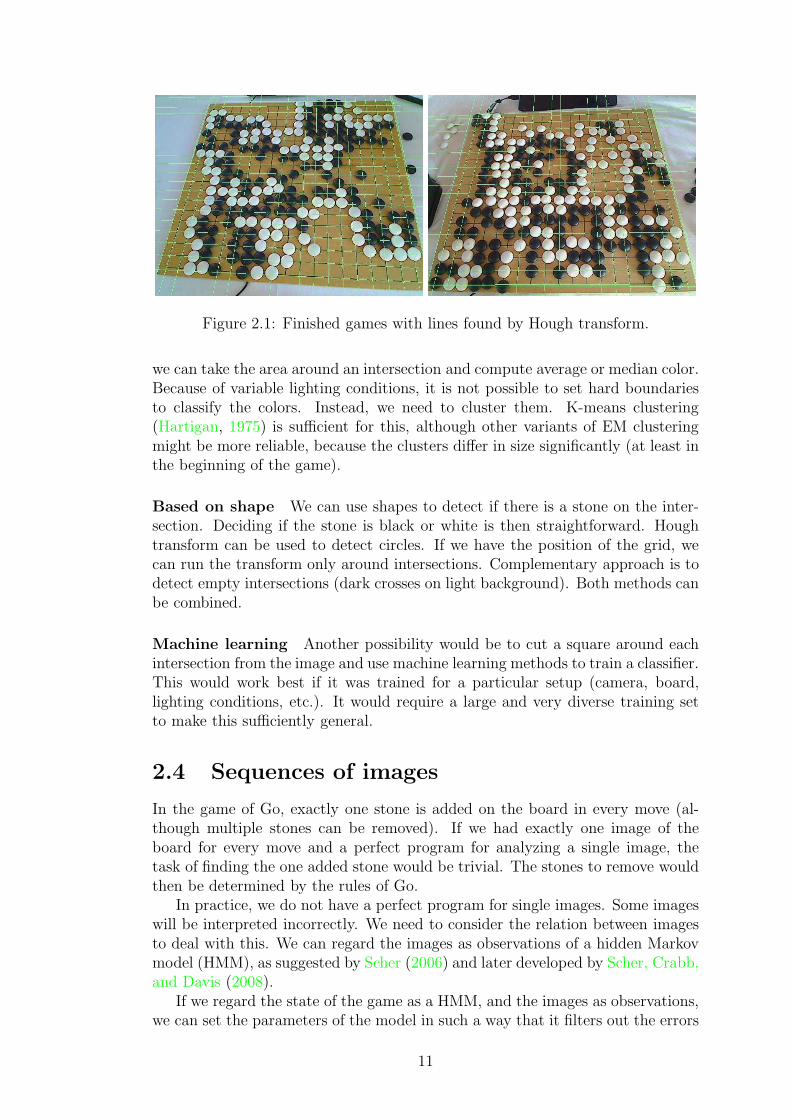
Figure 2.1: Finished games with lines found by Hough transform.

we can take the area around an intersection and compute average or median color.Because of variable lighting conditions, it is not possible to set hard boundariesto classify the colors. Instead, we need to cluster them. K-means clustering(Hartigan, 1975) is sufficient for this, although other variants of EM clusteringmight be more reliable, because the clusters differ in size significantly (at least inthe beginning of the game).

Based on shape We can use shapes to detect if there is a stone on the inter-section. Deciding if the stone is black or white is then straightforward. Houghtransform can be used to detect circles. If we have the position of the grid, wecan run the transform only around intersections. Complementary approach is todetect empty intersections (dark crosses on light background). Both methods canbe combined.

Machine learning Another possibility would be to cut a square around eachintersection from the image and use machine learning methods to train a classifier.This would work best if it was trained for a particular setup (camera, board,lighting conditions, etc.). It would require a large and very diverse training setto make this sufficiently general.

2.4 Sequences of images

In the game of Go, exactly one stone is added on the board in every move (al-though multiple stones can be removed). If we had exactly one image of theboard for every move and a perfect program for analyzing a single image, thetask of finding the one added stone would be trivial. The stones to remove wouldthen be determined by the rules of Go.

In practice, we do not have a perfect program for single images. Some imageswill be interpreted incorrectly. We need to consider the relation between imagesto deal with this. We can regard the images as observations of a hidden Markovmodel (HMM), as suggested by Scher (2006) and later developed by Scher, Crabb,and Davis (2008).

If we regard the state of the game as a HMM, and the images as observations,we can set the parameters of the model in such a way that it filters out the errors

11

in image analysis. For short games or smaller boards, the Viterbi algorithm(Viterbi, 1967) can be used to find the most probable order of the moves giventhe observations. For complete games on a 19× 19 board, the state space is toolarge for an exhaustive search and we need to heuristicaly prune it.

2.5 Video

To analyze a video recording, we can just treat it as a sequence of images. It wouldbe beneficial to detect and discard frames containing object (such as player’shand) moving over the board. This can be easily achieved by computing thedifference between consecutive images.

If we end up discarding too much frames (e.g. in a recording of a blitz game,when players are constantly moving their hands over the board), we can useoptical flow estimation (Sun et al., 2010) to find areas of strong movement. Wethen restrict our analysis to the static regions of each frame. Partial observationsare sufficient for HMM estimation.

There is also a question of analyzing a live video stream (e.g. for broadcastingan important tournament game over the internet). The software built for thistask needs to be very fast as well as reliable. The precision of such a systemwould be reduced by the fact that it would only know about past observationsand could not alter its decisions in situations such as detecting a conflict withthe rules and deciding that one of the past observations was flawed.

12

3. Related works

In this chapter we provides an overview of relevant academic work and currentlyavailable software.

3.1 Academic work

Optical recognition of Go position is an uncommon topic in academic writing.Only recently there has been a few papers published, the oldest we found datingfrom 2004.

None of the works mentioned below has publicly available working implemen-tation.

Srisuphab et al. (2012) describes AutoGoRecorder, an application for liverecording of Go games and record database management. It finds the boardat the beginning of the recording and assumes the position does not change.The camera must be positioned directly above the board. The average color inHSV color space measured in circular area around intersection is used to detectstones. Movement detection is used to select the frames in which the boardshould be checked for changes. There is no evaluation of the performance andthe application itself is not available.

Seewald (2010) presents a system based on machine learning methods. Thecorpus of images on which the system is trained and evaluated was created witha custom 8× 8 board. There is no reason to assume that this approach can workfor other users, unless everyone creates their own dataset and trains their ownclassifier specifically for their board and camera.

Scher (2006) proposes a method to improve a weak single-image classifier bytaking the whole sequence of images into account. The images are treated asobservations of states of a Hidden Markov Model. The Viterbi algorithm is used tofind the most probable sequence of states. This approach can be used to improveany system that works on single images. This method can be further developedby using the A* algorithm to search the space of possible move sequences (Scheret al., 2008).

Kang et al. (2005) and Yanai and Hayashiyama (2006) both proposealgorithms to extract game records from Go TV shows. Both works rely on theassumption that the video is recorded with a camera positioned directly abovethe Go board. This means that there is no perspective transformation and ver-tical lines on the board are also vertical in the image (and the same holds forhorizontal lines). This is a standard setup in TV broadcast of Go events, but itsuse anywhere else is very limited. It is fairly easy to analyze images under suchstrict assumptions and both works deal mainly with methods of selecting correctframes from the TV broadcast.

13

Hirsimaki (2005) describes a MATLAB prototype of a system for recognizingGo positions in single images. It is based on Hough transform. The two sets ofparallel lines are found by projecting the Hough space onto the angle axis andlocating two peaks. Small sub-grid is selected in the estimated center of the grid.The sub-grid is then grown until it fills the whole grid. The stones are classified byaverage luminosity around intersection. The output of the prototype consists ofan image with marked grid and stones, no abstract representation of the positionis given. The performance was evaluated on six images that can be downloadedwith the prototype.

The C++ implementation is also available1, but there was no update since2008. We were not able to compile it, but is clearly intended to only output imagewith marked situation, just as the prototype.

Shiba and Mori (2004) suggest to use a genetic algorithm to find the con-tour of the board in the image. They consider this being the first step towardsextracting the game position from images, but do not deal with subsequent steps(grid and stone location) at all.

3.2 Available software

There is a lot of software that attempts to automate Go game recording. Unfortu-nately, most of it is not complete and it is unmaintained and poorly documented.In this section, we survey available programs, the principles they work on andtheir current state of development.

Lot of the applications require to specify grid position manually and there-fore we cannot compare their performance with our work, which solves a harderproblem.

Rocamgo2 only works with video. It finds the corners of the grid (and assumesthe camera does not move). Then it applies the reverse perspective transformand finds the stones in the normalized image. Unfortunately, the stone-findingpart seems to be very unreliable. In a video with 30 first moves of a game, itonly found 22 moves and their order was entirely wrong. The documentation is inSpanish, therefore we do not know what principles it works on, apart from whatis obvious from the images displayed when the program is running.

MHImage/BenjaminsBox Go Image Recognition3 can analyze video, butrequires user to manually select proper frames, indicate the grid and manuallycalibrate stone recognition.

image2sgf4 requires user to supply coordinates of the corners of the grid. Itquantizes colors to classify the position. It was last updated in 2009.

1http://koti.kapsi.fi/thirsima/gocam/2http://github.com/Virako/Rocamgo3http://www.public.iastate.edu/~bholland/project_archive_content/

GoImageRecognition.html4http://www.inference.phy.cam.ac.uk/cjb/image2sgf.html

14

ludflu/kifu5 finds all closed polygons with 4 sides, it keeps those with areaaround median and computes the convex hull. Implementation is not finished,last update was made in 2012. See Figure 3.1 for result of the computation onone image from our dataset.

Figure 3.1: Screenshot of ludflu/kifu.

Kifu6 starts by finding a big quadrilateral shape. It assumes that is the board,cuts it from the image and uses Hough transform to find the lines. The programrelies on the assumption of static board and camera. The homepage claims that itworks on video, but the documentation7 does not describe how to choose relevantframes. It seems to be no longer maintained and it can no longer be downloaded.

Go Tracer8 is a web application. It asks the user to manually indicate theposition of the grid. After that, it clusters the colors around intersections andproduces a diagram. The color classification seems to be quite unstable.

Kifu-Snap9 is an Android application. The processing is done on the phone.

Go Scoring Camera10 is an Android application for automatic counting ofthe score. Processing is done on a remote server. Both this and Kifu-Snap arepaid and neither one is extensively documented.

5http://github.com/ludflu/kifu6http://www.sourceforge.net/projects/kifu7http://wiki.elphel.com/index.php?title=Kifu:_Go_game_record_(kifu)_generator8http://go-tracer.appspot.com/9http://remi.coulom.free.fr/kifu-snap/

10https://play.google.com/store/apps/details?id=com.jimrandomh.

goscoringcamera

15

Compogo11 was a SGF file editor for Windows, that was able to analyze seriesof images, given the position of the grid. The development was stopped in 2003.

Go Game Recorder12 webpage has a video demonstration, but no actualsoftware or source code. It was last updated in August 2013.

Go Watcher13 webpage also has a video demonstration, but no actual software.

11http://senseis.xmp.net/?CompoGo12https://gogamerecorder.wordpress.com13http://www.gowatcher.com/

16

4. Game position recognition

In this chapter we explain our solution and give an example of image analysis.The most significant difference from previous works is our use of RANSAC inthe analysis of Hough transform and in subsequent proccess of finding the grid.Another significant improvement is the use of clustering in the stone findingphrase. We also propose a new method for analysing video.

4.1 Finding the grid

In Figure 4.1 on page 19 we see the input image. It was taken by a webcameraconnected to the computer that can be seen in the top of the image. The computerwas running a Go clock and taking a picture each time a player pressed the keyafter his move. This method of recording lets the players to focus on the game(as tournament players are already used to playing with clock).

First we convert the image to gray-scale by computing luminance for eachpoint. To reduce the amount of noise in the subsequent Hough transform, weapply edge detection. We assume the lines are dark on light background, there-fore we use a simple filter with Laplace operator, followed by a high-pass filter(Fig. 4.2).

Next we take the Hough transform (Fig. 4.3, p. 20). Bright points in theHough transform represent strong lines in the image. The Hough transform isagain followed by a high-pass filter. If the lines are not strong enough, we canuse a filter similar to the one we used for edge detection (only with flipped signs)between the Hough transform and high-pass filter. This results in small groups ofnon-zero pixels, so we find connected components in the image and replace eachof them with its center. This way, we get one point in Hough space for each linein the image.

The grid is formed by two sets of parallel lines, so we are searching for twolines in the Hough space. We use RANSAC to find them (Fig. 4.4). We usestandard RANSAC to find the first line, we delete the points that lie on it andthen we use RANSAC again to find the second line. It would be possible toformulate a model with two lines, but it would need many more iterations to getthe right solution.

In Figure 4.5 on page 21 we see the selected lines over the original image.Now we find the candidates for the center of the grid. We make use of the

fact that we have most of the lines, therefore most of their intersections. If weexclude the lines that we already have, the lines that contain most points are thediagonals of the grid. We use RANSAC to find them (Fig. 4.6).

Once we have candidates for the diagonals, we can generate candidates forthe grid. We take an intersection on a diagonal as a corner of the grid. Becausewe have the lines and the other diagonal, we can compute position of remainingcorners and therefore the whole grid. We repeat this for all the intersections onall the candidates for diagonals and select the best grid (Fig. 4.7, p. 22). Thegrid candidates are scored in the same way as models in MSAC: for each of theintersections found in the previous step we count its distance to the nearest lineof the grid if it is smaller than δ and δ otherwise. We found that δ = 2 works

17

well for our application.

4.2 Finding the stones

For each intersection in the grid, we take average color in a 5 × 5 pixels squarearound it. In Figure 4.8 we see the average colors distributed in a color space,where the horizontal axis represent luminance and the vertical axis representsaturation.

We cluster the colors into three clusters using k-means clustering (Fig. 4.9,p. 23). The leftmost cluster corresponds to black stones, the rightmost to whitestones. The middle cluster corresponds to empty intersections.

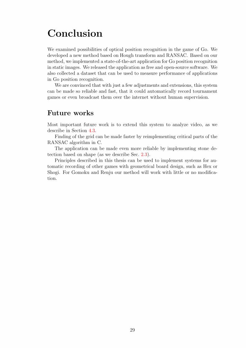
Once we have assigned stones to intersections, we can print the result as inFigure 4.10.

4.3 Video

In this section, we discuss our proposal for the video-analysis extention of thework described above. This exceeds the range of the implementation part of thisthesis and its realization is left for future works.

Trying to select precisely the frames in which we can observe the state ofthe board between moves and then analizing them without mistakes seems likea very unreliable approach. Therefore we propose to follow Scher et al. (2008)and use a HMM to model the game. As the state-space is quite large (up to 361M

where M is number of moves in the game), it is not feasible to compute the bestpath with Viterbi algorithm. Scher et al. (2008) find a good path with modifiedA* algorithm. We propose to search the state space with Monte-Carlo TreeSearch (MCTS, Coulom (2006)) instead. MCTS was already used in computer Goprograms with great success. There are open-source implementations of MCTSthat already contain Go rules, modifying one to count with probabilities insteadof number of wins should be straightforward.

18

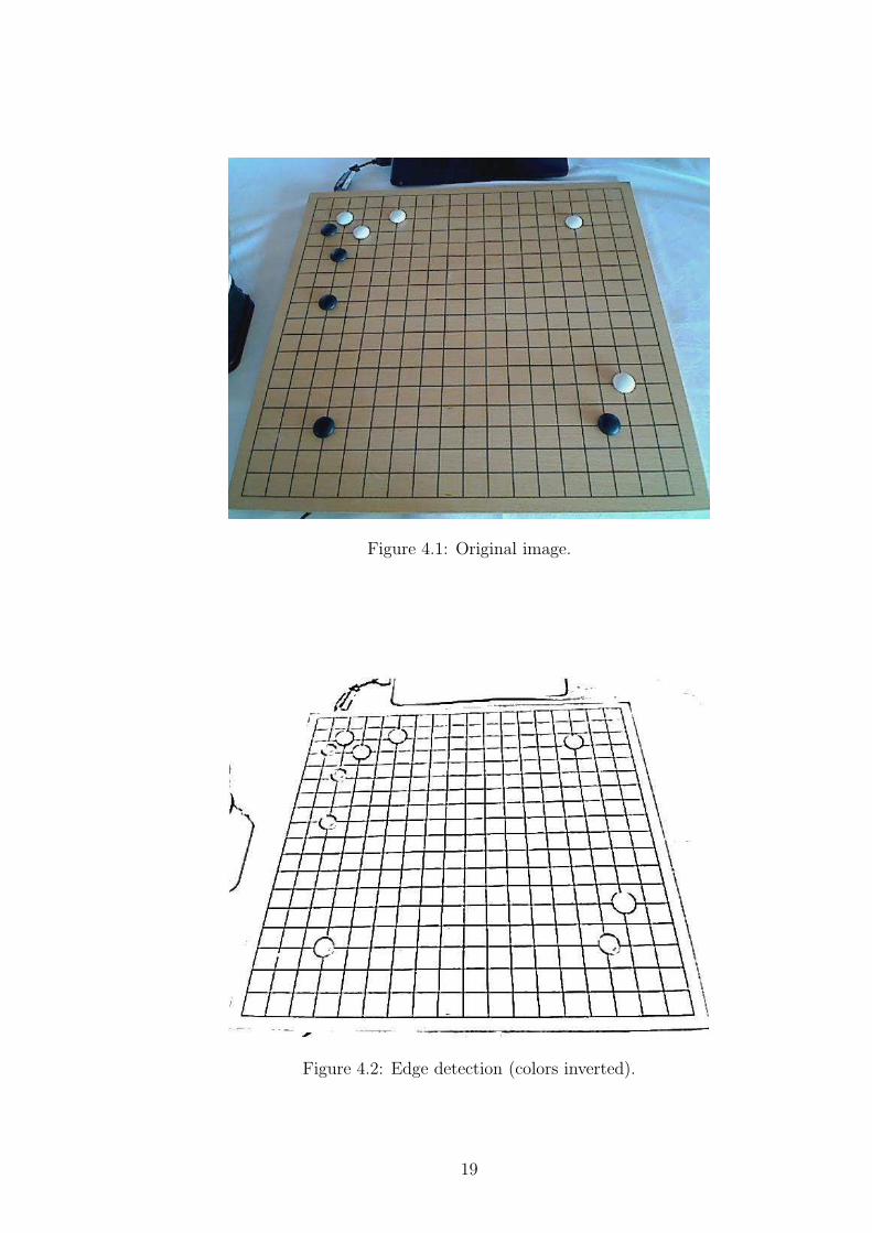
Figure 4.1: Original image.

Figure 4.2: Edge detection (colors inverted).

19

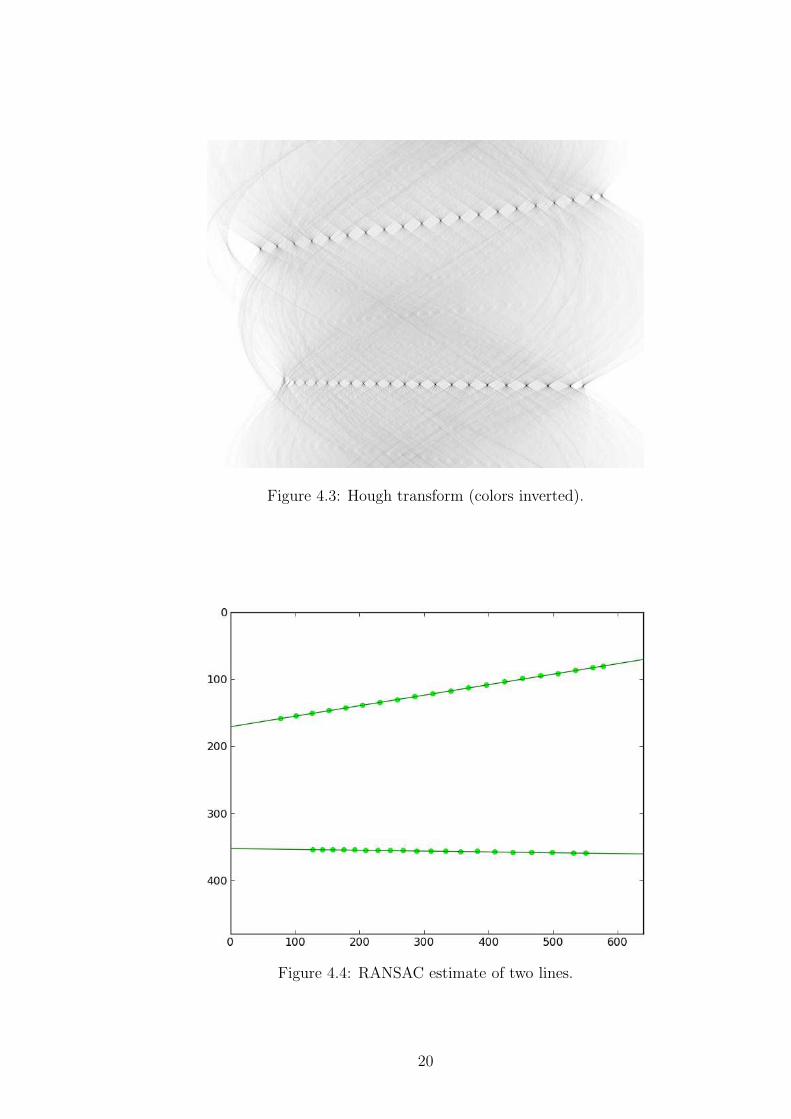
Figure 4.3: Hough transform (colors inverted).

Figure 4.4: RANSAC estimate of two lines.

20

Figure 4.5: Lines over the original image.

Figure 4.6: Finding the center.

21

Figure 4.7: The grid.

Figure 4.8: Distribution of the color around intersections.

22

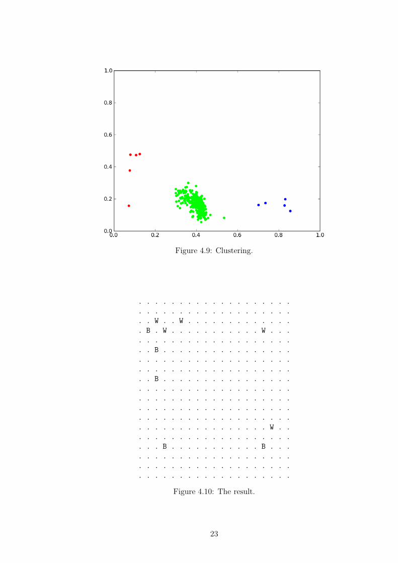
Figure 4.9: Clustering.

. . . . . . . . . . . . . . . . . . .

. . . . . . . . . . . . . . . . . . .

. . W . . W . . . . . . . . . . . . .

. B . W . . . . . . . . . . . W . . .

. . . . . . . . . . . . . . . . . . .

. . B . . . . . . . . . . . . . . . .

. . . . . . . . . . . . . . . . . . .

. . . . . . . . . . . . . . . . . . .

. . B . . . . . . . . . . . . . . . .

. . . . . . . . . . . . . . . . . . .

. . . . . . . . . . . . . . . . . . .

. . . . . . . . . . . . . . . . . . .

. . . . . . . . . . . . . . . . . . .

. . . . . . . . . . . . . . . . W . .

. . . . . . . . . . . . . . . . . . .

. . . B . . . . . . . . . . . B . . .

. . . . . . . . . . . . . . . . . . .

. . . . . . . . . . . . . . . . . . .

. . . . . . . . . . . . . . . . . . .

Figure 4.10: The result.

23

5. Implementation

In this chapter we describe Imago, our application for optical recognition of Gogame positions. Section 5.1 offers general description of the application. InSection 5.2 we discuss high-level technical choices we made. Detailed developerdocumentation is distributed with Imago and can be found on the attached CD(see page 33).

5.1 Imago

Imago is a program for automatic processing of Go images. It takes an image(or a set of images), finds the board-grid and stones and produces an abstractrepresentation of the game situation (or a game record).

It supports JPEG, BMP, TIFF (and other) image formats on input. It iscapable of output to ASCII and SGF format. As the process should be fullyautomatic, the program is operated from command line. There is, however, a GUIfor manual grid location in case the automatic one should fail.

The program is written mainly in Python, with performance-critical partswritten in C. It is distributed under slightly modified BSD 3-Clause License1.

The source code is available on GitHub2.

5.2 Technical documentation

Libraries and other dependencies

Most of the program is written in Python 2, so the Python 2 interpreter is neededto run it. Python development files and C compiler are needed to compile ourpcf module.

Beside Python’s standard library, we use PIL3 (or a compatible library, likePillow4) for image manipulation and numpy5 (Van Der Walt et al., 2011) forarray computations and linear algebra. These libraries should be sufficient forbasic functionality of Imago. For showing intermediate computations and plots,matplotlib6 is needed. Graphical user interfaces are implemented with pygame7.For capturing images with a camera we use OpenCV8 (Bradski, 2000).

Conventions

image coordinates The coordinates of the image start in the top left cornerwith [0, 0]. Fist coordinate is horizontal, second is vertical.

1http://opensource.org/licenses/BSD-3-Clause2http://github.com/tomasmcz/imago3http://www.pythonware.com/products/pil/4http://python-pillow.github.io/5http://www.numpy.org/6http://matplotlib.org/7http://www.pygame.org/8http://opencv.org/

24

lines We use multiple representations for lines, depending on the context. Linesrepresented by two points are easy to draw into image. For geometric computa-tions (distance from a point, intersection of two lines, etc.) we represent lines bycoefficients of the linear equation in general form (ax + by + c = 0). Lines weget from the Hough transform are represented by pairs (θ, d), where θ is anglebetween 0 and π and d is the distance from the centre of the image. The distancecan be negative, so that all parallel lines have the same θ and differ only in d.

colors There are two different representations of colors, one with discrete valuesfrom 0 to 255 for each channel, the other with floating point number between 0and 1 for each channel. We mostly use the former, but some libraries (matplotlib,colorsys from the Python standard library) use the latter, therefore we need toconvert between them sometimes. For gray-scale images we use discrete valuesbetween 0 and 255.

Most important modules

We give a high-level overview of the program architecture here. The detaileddocumentation is distributed with the program and can be found on the attachedCD.

imago.py This is the main module of the program. It contains the user interface.

linef.py This module finds the lines in the image.

gridf.py This module finds the grid, given the lines.

intrsc.py This module finds the stones on the grid.

hough.py This module implements the Hough transform.

ransac.py This module implements the RANSAC algorithm.

k means.py This module implements k-means clustering.

pcf.c This is a Python module written in C, that contains functions that are crit-ical for fast performance (e.g. the image processing part of Hough transformthat is called from hough.py).

Input and output formats

Imago loads images via PIL. It can open any image format, that is supported byPIL (JPEG, BMP, TIFF, . . . ).

Output for single images is a simple textual board representation with ’.’for empty intersection, ’B’ and ’W’ for black and white stones. See Figure 4.10on page 23 for an example. For game records, resulting from analysis of imagesequences, we use SGF file format. Single game positions can also be writtenwith SGF setup syntax.

25

SGF file format SGF9 (Smart Game Format) is the de facto standard fileformat for Go game records. Each move is recorded by its color (B or W), followedby coordinates in square brackets. The axes are labeled with letters from a to s.

There are a number of software packages for reviewing and editing Go SGFfiles (see article on Sensei’s Library10).

(;

SZ[19] HA[0] ST[0]

PB[Shusaku] PW[Gennan Inseki]

KM[0.0] RE[B+2]

BR[4d] WR[8d]

C[Gennan Inseki(white) VS Shusaku(black)]

;B[qd];W[dc];B[pq];W[oc];B[cp];W[cf];B[ep];W[qo];B[pe];W[np]

;B[po];W[pp];B[op];W[qp];B[oq];W[oo];B[pn];W[qq];B[nq];W[on]

;B[pm];W[om];B[pl];W[mp];B[mq];W[ol];B[pk];W[lq];B[lr];W[kr]

;B[lp];W[kq];B[qr];W[rr];B[rs];W[mr];B[nr];W[pr];B[ps];W[qs]

;B[no];W[mo];B[qr];W[rm];B[rl];W[qs];B[lo];W[mn];B[qr];W[qm]

)

Figure 5.1: Example of a SGF file — first 50 moves of a game.

Requirements for input images

We expect that:

• the board is standard 19 × 19 Go board, it has dark lines on light back-ground,

• the board is completely visible — it does not exceed the image,

• no part of the board is obscured by player’s hands or other object gettingbetween the board and the camera,

• the image is reasonably sharp and the perspective is not exceedingly dis-torted,

• the resolution of the image is at least 640× 480 pixels, and

• the board takes up most of the image — at least half of the shorter dimen-sion of the image.

We do not have have any special requirements on camera angle and lightingconditions. If the image meets the criteria above and the position can be rec-ognized by a human without difficulties, then the computer should be able torecognize it as well. The program might work even if the image violates some ofthe above mentioned conditions, but it is not guaranteed to.

9http://www.red-bean.com/sgf/10http://senseis.xmp.net/?SGFEditor

26

6. Evaluation

In this section we evaluate the performance of Imago. We have not found anyother work that we can meaningfully compare our results with (see Chapter 3for details). Therefore we build our own dataset, that we describe in Section 6.1.Results of our experiments on the dataset are given in Section 6.2.

6.1 Dataset

There is no standard dataset for measuring performance in optical position recog-nition in Go. We collected a set of images and manually recorded their gamepositions. We hope that this dataset can be used as a basis of comparison forany future works in this area, despite its small deficiencies: Even though we triedto make the dataset diverse, we only had two different cameras and two differentGo boards at our disposal. Because Imago was tested on this dataset during de-velopment, it would have to be expanded or replaced by an independent datasetto make the comparison with Imago fair.

We also recorded two complete games, with an image taken after each move.These can be used to experiment with extracting game records from image se-quences.

6.2 Experimental results

Precision

The dataset consists of 55 images. We run the test 3 times, because parts of thealgorithm are stochastic and results may vary.

mistakes no mistakes

incorrect one two threegrid stone stones stones

1 0 (0.0%) 3 (5.5%) 5 (9.1%) 5 (9.1%) 42 (76.4%)2 0 (0.0%) 3 (5.5%) 5 (9.1%) 5 (9.1%) 42 (76.4%)3 0 (0.0%) 3 (5.5%) 5 (9.1%) 5 (9.1%) 42 (76.4%)

Table 6.1: Test results on our dataset.

As we see in Table 6.1, Imago gives consistent results. The position of thegrid was always determined correctly. There are a few images in which Imagomisclassified up to three stones, but never more than that. Most of the images (76%) were classified with no mistakes. If we employed a measure counting with thetotal number of intersections, Imago would have 99.9% accuracy on this dataset.

Detailed reports of test results can be found on the attached CD.We also evaluated a version of Imago based on Cuckoo Search. With high

number of iterations, the number of correctly determined grid positions was alsonearly 100 %, but the analysis took on average 240 seconds for an image.

27

Time consumption

On Intel Core2 Quad Q6600 (2.40GHz) CPU it takes 28 seconds on averageto analyze an image from our dataset. Most of the time is spent finding thediagonals with our variation of RANSAC algorithm. To reduce the time consumedby this part of the analysis, we can reduce the number of RANSAC iterations.In Table 6.2 we see how this affects the precision of our system. The time isreduced linearly with the decreasing number of iterations. Error rate increasessignificantly under 200 iterations. In the other direction, error rate decreasesslowly and we need at least 800 iterations to consistenly achieve 0 mistakes onour dataset. This behavior was anticipated, because 200 iterations is the expectedamount needed to find the correct diagonal line.

iterations 800 500 200 150 100grids not found 0 (0.0%) 1 (1.8%) 2 (3.6%) 9 (16.4%) 14 (25.5%)average time [s] 28 20 13 12 10

Table 6.2: The effect of number of RANSAC iterations on time and precision.

Another way to make our application faster is to rewrite our RANSAC im-plementation from Python to C.

28

Conclusion

We examined possibilities of optical position recognition in the game of Go. Wedeveloped a new method based on Hough transform and RANSAC. Based on ourmethod, we implemented a state-of-the-art application for Go position recognitionin static images. We released the application as free and open-source software. Wealso collected a dataset that can be used to measure performance of applicationsin Go position recognition.

We are convinced that with just a few adjustments and extensions, this systemcan be made so reliable and fast, that it could automatically record tournamentgames or even broadcast them over the internet without human supervision.

Future works

Most important future work is to extend this system to analyze video, as wedescribe in Section 4.3.

Finding of the grid can be made faster by reimplementing critical parts of theRANSAC algorithm in C.

The application can be made even more reliable by implementing stone de-tection based on shape (as we describe Sec. 2.3).

Principles described in this thesis can be used to implement systems for au-tomatic recording of other games with geometrical board design, such as Hex orShogi. For Gomoku and Renju our method will work with little or no modifica-tion.

29

Bibliography

Dana H Ballard. Generalizing the hough transform to detect arbitrary shapes.Pattern recognition, 13(2):111–122, 1981.

William A Barrett and Kevin D Petersen. Houghing the hough: Peak collectionfor detection of corners, junctions and line intersections. In Computer Visionand Pattern Recognition, 2001. CVPR 2001. Proceedings of the 2001 IEEEComputer Society Conference on, volume 2, pages II–302. IEEE, 2001.

Robert Charles Bell. Board and table games from many civilizations, volume 1.Courier Dover Publications, 1979.

G. Bradski. The opencv library. Dr. Dobb’s Journal of Software Tools, 2000.

Remi Coulom. Efficient selectivity and backup operators in monte-carlo treesearch. In In: Proceedings Computers and Games 2006. Springer-Verlag, 2006.

Richard O Duda and Peter E Hart. Use of the hough transformation to detectlines and curves in pictures. Communications of the ACM, 15(1):11–15, 1972.

Martin A Fischler and Robert C Bolles. Random sample consensus: a paradigmfor model fitting with applications to image analysis and automated cartogra-phy. Communications of the ACM, 24(6):381–395, 1981.

John A Hartigan. Clustering algorithms. 1975.

T Hirsimaki. Gocam: Extracting go game positions from photographs. HelsinkiUniversity of Technology, Helsinki, Finland, Tech. Rep, 2005.

Paul VC Hough. Method and means for recognizing complex patterns, Decem-ber 18 1962. US Patent 3,069,654.

Kaoru Iwamoto. Go for beginners. Ishi Press, 1972.

George H Joblove and Donald Greenberg. Color spaces for computer graphics.In ACM siggraph computer graphics, volume 12, pages 20–25. ACM, 1978.

Deuk Cheol Kang, Ho Joon Kim, and Kyeong Hoon Jung. Automatic extractionof game record from tv baduk program. In Advanced Communication Technol-ogy, 2005, ICACT 2005. The 7th International Conference on, volume 2, pages1185–1188. IEEE, 2005.

J Kennedy and R Eberhart. Particle swarm optimization. In Neural Networks,1995. Proceedings., IEEE International Conference on, volume 4, pages 1942–1948. IEEE, 1995.

Frank O’Gorman and MB Clowes. Finding picture edges through collinearity offeature points. Computers, IEEE Transactions on, 100(4):449–456, 1976.

Steven Scher. Recording a game of go: Hidden markov model improvesa weak classifier. http://classes.soe.ucsc.edu/cmps290c/Winter06/

proj/stevenreport.doc, 2006. Accessed: 9. 7. 2014.

30

Steven Scher, Ryan Crabb, and James Davis. Making real games virtual: Trackingboard game pieces. In Pattern Recognition, 2008. ICPR 2008. 19th Interna-tional Conference on, pages 1–4. IEEE, 2008.

Alexander K Seewald. Automatic extraction of go game positions from images:A multi-strategical approach to constrained multi-object recognition. AppliedArtificial Intelligence, 24(3):233–252, 2010.

Pranab Kumar Sen. Estimates of the regression coefficient based on kendall’stau. Journal of the American Statistical Association, 63(324):1379–1389, 1968.

Kojiro Shiba and Kunihiko Mori. Detection of go-board contour in real imageusing genetic algorithm. In SICE 2004 Annual Conference, volume 3, pages2754–2759. IEEE, 2004.

Milan Sonka, Vaclav Hlavac, and Roger Boyle. Image processing, analysis, andmachine vision. Cengage Learning, 2014.

A Srisuphab, P. Silapachote, T. Chaivanichanan, W. Ratanapairojkul, andW. Porncharoensub. An application for the game of go: Automatic live gorecording and searchable go database. In TENCON 2012 - 2012 IEEE Region10 Conference, pages 1–6, Nov 2012.

Deqing Sun, Stefan Roth, and Michael J Black. Secrets of optical flow estimationand their principles. In Computer Vision and Pattern Recognition (CVPR),2010 IEEE Conference on, pages 2432–2439. IEEE, 2010.

Phil Torr and Andrew Zisserman. Robust computation and parametrization ofmultiple view relations. In Computer Vision, 1998. Sixth International Con-ference on, pages 727–732. IEEE, 1998.

Philip HS Torr and Andrew Zisserman. Mlesac: A new robust estimator withapplication to estimating image geometry. Computer Vision and Image Un-derstanding, 78(1):138–156, 2000.

Stefan Van Der Walt, S Chris Colbert, and Gael Varoquaux. The numpy ar-ray: a structure for efficient numerical computation. Computing in Science &Engineering, 13(2):22–30, 2011.

Andrew J Viterbi. Error bounds for convolutional codes and an asymptoticallyoptimum decoding algorithm. Information Theory, IEEE Transactions on, 13(2):260–269, 1967.

Keiji Yanai and Takehisa Hayashiyama. Automatic” go” record generation froma tv program. In Multi-Media Modelling Conference Proceedings, 2006 12thInternational, pages 4–pp. IEEE, 2006.

Xin-She Yang and Suash Deb. Cuckoo search via levy flights. In Nature &Biologically Inspired Computing, 2009. NaBIC 2009. World Congress on, pages210–214. IEEE, 2009.

Marco Zuliani. Ransac for dummies. http://vision.ece.ucsb.edu/~zuliani/Research/RANSAC/docs/RANSAC4Dummies.pdf, 2014. Accessed: 13. 7. 2014.

31

A. User documentation

Installation

Make sure you have all dependencies installed. That is PIL (or equivalent) andnumpy for basic functionality, matplotlib, pygame and OpenCV for additionalfeatures. On a Debian-based system, you can just run sudo apt-get install

python python-dev python-imaging python-numpy python-matplotlib

python-pygame python-opencv. Most of the libraries can be also installed withPIP, except for pygame, which has to be downloaded from its website.

Once you have all the dependencies, you need to compile Imago C code. Runmake in the imago directory. Imago should now be ready to run.

User guide

Command line interface

Using Imago is easy. Just run ./imago image.jpg to extract the position fromimage.jpg. If you specify multiple images, Imago will find the grid in the firstone and extract the game record, assuming that the board position does notchange, and images are in the correct order with one image per move. With./imago -S <files> the game record is produced in SGF. Run ./imago -h forhelp and the list of all options.

Graphical user interface

The goal of this work is to make Go recording as automatic as possible. Asa result, we expect minimum of user interaction. Therefore we decided to designour graphical user interfaces in rather minimalist way.

Manual grid selection You can select the grid manually, by running ./imago

-m <file> [more files].

Camera, Go timer There are two helper programs to facilitate taking of pho-tographs during the game. The ./imago-camera command, that takes images atthe press of the key or automatically with selected interval. And ./imago-timer,that displays Go game clock and takes an image with every clock-press. For de-tailed instructions on setting the time limits and video device attributes, run thecommand with -h option.

32

B. The attached CD

The content of the attached CD:

• source code of the implemented software (imago),

• developer documentation (documentation),

• a dataset consisting of images and text files with corresponding positions(imago/test_data),

• detailed test results (imago/test_data), and

• a PDF file with this thesis (thesis.pdf).

All the materials can also be found on the webpage of the Imago project1.

1http://tomasm.cz/imago

33