1

Openness and growth in alternative trading regimes. Evidence from EEC and CMEA’s customs unions

Rosa Capolupo* Giuseppe Celi

University of Bari, Department of Economics, Via Camillo Rosalba 53, Bari, (Italy) and University of Glasgow, Department of Economics,

Adam Smith Building, Glasgow G12 8RT (UK)

Abstract

While common sense would indicate that trade and growth are positively correlated, it is not clear from a theoretical and empirical perspective whether or not trade is a proximate determinant of growth. The voluminous empirical efforts in this area show mixed findings. Trying to elucidate the ambiguities in the literature we study the nexus between trade flows and growth in three groups of countries: historical EEC, the extreme case of CMEA customs union and a group of transitional economies (TEs), most of which just recently added to the EU member states. The comparator group of former communist countries, in which trade-openness is not spurred by market incentives, should be very informative in explaining the impact of trade on growth. Our main finding, by applying different econometric methodologies, is that either for the EEC or CMEA the coefficient of real openness is negative for the former two samples and positive for the third. For the EEC the indicator of openness shows a positive sign solely when the rate of growth of trade share is considered. The findings prove to be robust to variations in the controlling set, to different econometric techniques, and for the last group of countries to changing in the empirical indicator of openness (inter and intra-industry trade indicators). Keywords: economic growths, transition economies, capital accumulation, trade Openness, panel data JEL: O47, O42, E22, Corresponding author: email:r.capolupo@dse.uniba.it

2

1. Introduction

The literature on the relationship between growth and international trade is very large and

has received a great boost with the appearance of models of endogenous growth in which trade

plays an important role in affecting long run growth through various channels. First, technology

diffusions and spillovers generated by improvement in knowledge may spread quickly through

trade-partner countries. The access through international trade to a wide variety of intermediate

goods and new final products will affect a country’s productivity growth (Grossman and

Helpman [1991], Aghion and Howitt [1992]. Second, trade and technological diffusion reduces

duplication of research effort and enlarges the size of the market in which the typical firm

operates. This raises the monopoly rents that can be appropriated by successful innovators

promoting research-intensive production [Grossman & Helpman [1991], Romer [1990] which

influences positively the growth rate. Third, there should be an indirect effect of international

trade that operates through competition among firms in outward-oriented countries. These pro-

competitive gains from trade will increase specialisation and the incentive to innovate with a

positive impact on growth.

Beyond these effects, however, there may exist a number of potentially counteracting

effects. The most relevant (Aghion and Howitt [1992], Grossman and Helpman [1991]) is that a

country, because of imitation in technology, might not be able to appropriate all the benefits

from their investment in new technology. Indeed, innovations will be incorporated in factors and

goods which are object of trade and imitation of the new technologies by follower becomes

easier. At the global level this is a positive effect but it is a negative externality for countries

which have devoted higher resources to R&D. Therefore, the new growth theories do not predict

that trade will unambiguously enhance the growth rate of economies. The results of positive

links between trade and openness will depend on whether or not the forces of comparative

3

advantage drives resources in the direction of activities that generate long run growth (via

externalities, quality upgrading, expanding product varieties).

From an empirical point of view, however, the majority of economists believes that there

is little question about the positive association of expanding trade and economic growth; see e.g.

Harrison (1996), Edwards (1993, 1998), Sachs and Warner (1995, 2001), Frankel and Romer

(1999), Miller and Upadhyay (2000), Wacziarg (2001), Wacziarg and Welch (2003), Irwin and

Tervio (2002), Alcalà and Ciccone (2004), among others.

In contrast to this view, the classical cross-section empirical study by Levine and Renelt

(1992) offers support for the link between trade and resources allocation (static efficiency) but

questions long run growth effects. More recently, an emerging literature, initiated by Rodriguez

and Rodrick (1999), Rodrick et al (2002), Vamvakidis (2002) and partly by Lee, Ricci and

Rigobon (2004), shows the inconsistency of previous results, which are sensitive to the proxy

variables of openness, data sets and samples of countries included in the analysis. Whereas in

some works the impact of trade volume on growth has been investigated, in others different

empirical proxies for trade policy orientation has been adopted. This last strand of literature,

aimed at assessing the effects of liberalisation on economic performance of developing countries,

shows weak results in the trade-growth link across countries. These findings have raised

questions about the reliability of canonical measures of trade policy in capturing the growth

benefits of outward orientation policy. (Dollar and Kraay [2003]1.

The present work draws from these researches trying to study the robustness of the nexus

between trade flows and growth in three groups of countries: historical EEC, the extreme case of

CMEA customs union and a group of transitional economies (TEs).

Taking into account econometric criticisms (parameter heterogeneity, explanatory power

of the regressions) as well as the conflicting empirical outcomes, we focus on panels of a

1 Dollar and Kraay report the case of China policy of trade decentralization with modest reduction in the official import tariffs. Other important examples of this policy can be find analysing trade policy of high growing East Asian countries. This suggest that is difficult to construct a single convincing index of trade policy.

4

relatively homogeneous set of countries that share a common set of relevant coefficients. Aside

from the difficulties of isolating trade policy, since it is not just this policy but many other

macroeconomic policies that affect growth, we share with Pritchett (2001) and Harrison (1996)

the view that trade flows are the best measure of trade orientation, capturing both inward oriented

and export promoting regimes. Hence, it should be informative to look at countries which have

grown steadily and appreciably in the last decades and in which trade is perceived to have been

historically an important factor of growth. Analogously, it should be of interest to look at

countries that when opened to international trade, i.e. after the communist regime and after a short

transition, are becoming important exporters and their growth patterns seem to follow the export-

led growth hypothesis. What Wacziarg and Welch (2003) have shown, by extending and updating

the Sachs and Warner (1995) openness indicator, is that these countries have immediately gained

the value of 1 in the binary measure, just after the falling off the iron curtain.

Although there have not been many studies underlying the growth effects of openness for

European countries, we would expect that integration between similar countries, as predicted by

endogenous growth theories, would enhance the growth rate of economies (Rivera Batiz and

Romer [1991])2. Casual empiricism shows that this took place for EECs at least until 1990 but not

for CMEA, which consist of the former planned economies defined as closed in the Sachs and

Warner sense3. Why has a customs union like CMEA4, in which the volume of intra-area trade has

2 The empirical paper by Henreksson et al (1997 shows that EC memberships have a positive effect on economic growth. The membership is valued in their regressions with a dummy and the authors themselves claim that it should not capturethe effects of European integration but other developed country characteristics. In addition the resuls are not completely robust to changes in the set of the control variables (Henrekson et al. p.1547)

3 According to Sachs and Warner (1995) an economy is closed if it satisfies one of the five conditions (1) tariffs of 40% or more; (2) quotas of 40% or more; (3) black market premium higher or equal to 20%; (4) country with a state monopoly in export; (5) a country with a socialist economic system. The high tariffs should be computed considering the mid 1970 and quotas the mid 1980. The Sachs and Warner indicator captures many aspects of openness and particularly commercial policies than just trade. As Harrison and Hanson (1999) state, of all the five factors described by Sachs and Warner in defining their trade measure, only the socialist system dummy variable seems to be negatively and significantly correlated with growth. 4 The CMEA (Council for Mutual Economic Assistance) includes Poland Hungary, Bulgaria, Romania, Czechoslovakia, East Germany, USSR, Mongolia, Vietnam Cuba, and Yugoslavia. For a detailed assessment of the CMEA trading system see Lavigne (1995), Schrenk (1992), Sheets and Boata (1996)

5

been very large, not produced the expected effects on the growth rates of the countries involved in

the trade agreement? The institution of the CMEA trading group had as an objective to use trade

within the planning system to guarantee a satisfying rate of growth across socialist countries. Is its

failure a confirmation that the degree of market incentives, payment systems, and institutional

variables that affect productivity growth are more important than trade flows as claimed by

Rodrick et al (2003) and Dollar and Kraay (2001)? An assessment of dissimilarities between the

two customs unions, one characterised by exceptional growth and the other by a great diversion of

resources, may shed some light on the trade-growth nexus. At the same time, it should be also

informative to explore why changing the composition, volume, and partners of trade, just after the

fall of the Berlin Wall, the higher degree of openness of former CMEAs with other EU members

resulted in high growth rates for the former, despite the enormous problems involved in the

process of transition. In the period 1985-1988 the average export shares of these countries5

towards EECs was about 24% and towards CMEAs 49.8%. In 1994 data indicated a substantial

increase of Eastern European Exports to EECs (52.8%) and a large decline to CMEAs (16.9%).

How countries with a low or modest level of technological progress are able to redirect their

export to the EECs if industrial restructuring, technological spillovers and search of comparative

advantages would require a longer span? We think that the theoretical arguments stressed can

have a partial response by looking at the changing process in Eastern Europe and at the role of the

structure of trade in these countries. We would expect, for this group that benefits on growth

come mainly by inter-industry trade flows. Our findings show instead an important and positive

role of intra-industry trade for TEs.

Even if the nexus trade-growth has been widely studied, the paper contributes to the current

debate at three levels. First, following the division into communist and market economies we test

implicitly the importance of institutional factors (monopoly power by the government, property

5 The countries to which the figures refer are Poland, Hungary, Bulgaria, Romania, Czechoslovakia. Data are from IMF Direction of Trade Data.

6

rights, distortions in resources allocation) on growth. Second, considering the methodological

issues raised by growth econometrics, the use of panel estimation techniques aids to investigate

the relationship more robustly. Third, the unsatisfactory results found for CMEAs and EECs led

us to find a finer measure (at a lower level of disaggregation) of openness by looking at the

structure of trade for the TEs.

The remainder of the paper proceeds as follows. In section 2 we briefly discuss data,

methodological issues and outline model specifications. In section 3 we perform empirical tests of

the effects of trade openness on economic growth for the two customs unions and present the

results. We proceed in section 4 by analysing the composition of trade for a group of transition

and accession countries (TEs) and perform regressions of different measures of inter and intra-

industry trade on growth rates. The last section concludes.

2. Data, samples, and methodological issues. In our analysis we use time series data taken mainly from the Penn World Tables, version

6.1. A detailed description of these data can be found in the Appendix as well as in Heston,

Summers and Aten (HS&A, 2002). Our data set contains the countries of the former European

Community as well as CMEA. The EEC sample and time series are historically updated by the

inclusion of countries in the year in which they joined the EC6.

The data set for the second panel covers the period 1960-1989 and is unbalanced since

data for some countries started in 1970. The countries included are all pertaining to CMEA

customs union7.

In the empirical growth literature the most commonly used econometric method has been

cross section estimation of the Barro and Sala-i-Martin (1995) style. This approach uses a single

regression and average-values of the variables and growth rates for each country for the entire

6 For example, data for the UK, Ireland and Denmark are included beginning in 1973. The data set for the first panel covers the period 1950-1990. From the sample we dropped Luxembourg which joined the EC from the beginning but that is a strong outlier for its high degree of openness.

7

period. It also assumes that the production function parameters and levels of technologies are the

same across countries. The emerging of a widespread dissatisfaction with this standard empirical

method of growth analysis has brought many researchers to partly overwhelm the criticisms by

adopting a procedure that accounts for country idiosyncratic effects. The approach of dynamic

panel estimations which deals with many of the econometric difficulties (controls for country

specific effects and endogeneity of regressors) arising in the earlier studies has been applied in

growth regressions by Caselli, Esquivel and Lefort (1996), Bond, Hoeffler and Temple (2001),

among others. The new stage in the empirics of growth has seen the replacement of the first

differenced General Method of Moments (GMM DIFF) of Arellano and Bond (1991), with

Arellano and Bover (1995) and Blundell and Bover (1998)’s GMM system8.

In this work we employ dynamic panel estimators together with standard techniques. We

apply panel estimators by using pooled data at annual frequency and also averages of five year-

periods as in the majority of studies on the subject. We are aware that there are some problems in

dealing with annual time series data. The first is that some variables, particularly human capital,

are measured every 5 years (Barro & Lee [2000] data set). The second is that cyclical fluctuations

may cause variations in short run growth rates. To overcome the first problem we calculate the

time series of human capital by interpolation and the second one by using longer lags of the

variables under studies. However, the results on the openness measure strongly differ when we

consider panel based on averages of five-year periods.

The starting specification of the empirical modelling is a standard cross-country growth

regression that can nest much of the existing literature on the empirics of growth:

itiitstiit Xyy εηβββ ++++= − 2,10 ' for i = 1,…, N and t = 2,…,T (1)

where yit denotes the natural logarithm of real per-capita GDP in country i at time t , yit-s is a

lagged income per capita, Xit is a vector of explanatory variables including our measure of

7 The other three countries of CMEAs, not in the European area, Vietnam, Cuba and Mongolia, have been dropped. 8 See Bond, Hoeffler and Temple (2001) for a discussion of the application of the two methodologies in growth analyses.

8

openness, ηi is the country specific intercept, such as unobserved factors that influence the

country growth rate, and εi,t is the disturbance term, which reflects shocks to the level of output

per capita. The error term and ηi are assumed to be uncorrelated and independently distributed

across countries (E (ηi,) = 0, and E (εi,t ηi ) = 0 ). Subtracting lagged income from both sides of

equation (1) yields the dynamic panel model in which the growth rate is regressed on controls and

lagged output:

itiitstistiit Xyyy εηβββ ++++=− −− 2,10, 'ˆ for i=1,…,N and t=2,…,T

(2) where )1(ˆ −= ββ . As already stated, the current methodology to deal with both

problems is Arellano and Bond (1991) framework. The equation above, rewritten in differences,

removes the fixed effects (and its potential correlation with lagged income variable) and allows

estimates by instrumental variables using appropriate lags of the regressors as instruments.

The specification, differencing equation (1) is:

)()(')( ,,22,,1, stiitstiitstististiit XXyyyy −−−−− −+−+−=− εεββ (3)

The DIF-GMM approach of equation (3) may lead to a large downward bias in the coefficients

when the time periods are too short with respect to the number of countries. Even if this is not the

case in this work, in which the number of time periods is almost equal to the number of countries,

we also perform GMM (SYS) estimations as a sensitivity analysis to check whether the results are

robust to change in the estimated methodology. The use of GMM-SYS involves estimating jointly

equations (3) in differences and (1) in levels by adding lagged differences of endogenous

variables as instruments for the equation in levels9. The additional moment conditions for the

regressions in levels are:

[ ] 10))(( ,1,, ==+− −−− sforyyE tiististi εη (4)

[ ] 10))(( ,1,, ==+− −−− sforXXE tiististi εη (5)

9 For details on the two methodologies see Arellano and Bover (1995), Blundell and Bond (1998), Bond et al (2001)

9

Unfortunately, this statistical tool also causes some problems. Both the necessity to construct lag

values and the addition of more regressors on the right end side will decrease the sample size and

the degree of freedom of the estimation. Another set of questions concerns serial correlation. Tests

for first and second order serial correlation are reported for each regression.

Results for CMEA and EEC’s Sample

3.1 The CMEA Sample

Following the methodological discussion above we present the results of our analysis. We

start by reporting results for the CMEAs and for the EECs. For each sample we present two tables

of results. The first table shows estimates with annual data and the second table describes the

results using data averages five-year periods.

Among the determinants of growth we will test different specifications of the basic

regression equation by including measure of real trade openness (OPEN), given by the ratio of

export plus import to GDP, and the set of regressors that researchers always consider in growth

regressions. These regressors are: the growth rate of population, the natural log of real investment

ratio I/Y, the natural log of real consumption government spending in GDP (G), and human

capital. This last variable will be denoted in specific regressions with PRIM, to indicate the

percentage of population which attains primary education, SECON for secondary education. We

will also use, in some specifications the variable AVERSCH as the stock measure in Barro and

Lee (2000) denoting the average years of schooling in the population of 25 years and above. In

some regressions interaction of human capital with investment and openness will be used and

such an interaction term will be denoted by EDU. We restrict the number of countries and the

period of observations from 1970-1990 for the CMEAs. Time periods, country-samples and

methodology adopted will be indicated for each regression.

The coefficient estimates of the basic regression are listed in column 1 of Table 1, which

illustrate results using annual data. We find a significant negative effect of trade on growth and a

positive relationship for the investment share. The estimated coefficient of ln of real investment to

10

GDP is positive and statistically significant at 1% level. The openness variable has a negative

impact and the coefficient is significant at 5% level. The other regressions differ not only for the

estimation techniques but also for the measures of human capital used. We performed regressions

with the various measures of human capital used in the literature and we find that only PRIM is

positively correlated with growth. All other measures even when have been interacted with

investment and openness10 exhibit the usual negative sign. However, the opinion of economists

about the importance of primary education is very dissimilar. Some economists (Klenow and

Rodriguez-Clare [1999]) argue that primary education is not very important for growth, others

(Psacharoupoulos[1994], Grier [2002]) claim that it is universally one of the most important

factors of development. The group of CMEAs is formed by countries that do not have a high level

of technology and the positive correlation of primary education with growth is common to results

found in other developing countries11. It should be noted that the introduction of the growth rate

of trade share as regressor is used in some specifications in order to verify if such measure, which

will reveal positive for EEC, should have a positive impact on growth also for this group of

countries. The sign remains negative in all regressions (not reported).

Table 1: Annual Data Cross-country Growth regression (1960-1990) CMEA Sample

Dependent Variable: ∆ln yt

Regressors (1)

OLS

(2)

OLSDV

(3)

2SLSIVa (4)

GMM(DIFF)

(5)

GMM(SYS)

Constant −0.12121

(−1.61)

0.03034

(0.61)

0.25061***

(2.39) −0.002803 **

(−2.49)

−0.116991*

(−1.68)

∆ln yt-s 0.179659**

(2.33)

0.278180***

(3.48)

10 We tried to interact human capital with openness and investment to estimate the effect of this interactions on growth rate. The

idea is that larger openness encourages the introduction of new technologies, increases the demand of high skilled workers with a

positive impact on learning by doing and productivity. This has suggested to include the interaction term plus the level of human

capital as a separate regressors (see Harrison [1996]).

11 It is worth noting that in a growth framework one should include the growth rate of human capital more than its level, but many researchers claim that the rate of accumulation of human capital is very slow and have modelled GDP growth as function of the level of human capital (Benhabib and Spiegel [1994, 2000]). However, when we introduce the rate of growth of human capital (primary, secondary and average years of schooling) the coefficients in our regressions turn out to be positive (not shown)

11

Ln (I/Y) 0.06942

(3.67)

0.00372***

(4.83)

0.09053***

(4.68) 0.1864113***

4.92

0.064353***

(3.44) Ln OPEN −0.05903

(−1.85)

− 0.001328

(-4.31)

−0.04022***

(− 4.06)

∆ln OPEN −0.0800985***

(−2.75)

−0.076507***

(−2.48)

PRIM 0.00080***

(2.80)

−0.0006653

(−0.89)

SECON −0.00094***

(−3.24)

(−0.018490***

(−2.55)

AVERSCH − 0.02195

(−1.13)

∆ln POP −1.28658

(−1.11)

−0.03124***

(−4.17)

0.3125058

(0.18)

− 1.13347

(−0.98)

Ln G −0.01302

(−2.15)

0.000388

(-0.28)

−0.006189

(−1.15)

Dummy1 −0.08126***

(-2.68)

Dummy3 −0.02950

(0.87)

Dummy4 −0.03633

(-1.03)

Dummy5 − 0.03285**

(−2.12)

Dummy6 − 0.05219**

(-2.46)

Dummy7 −0.02138

(− 0.75)

Dummy8 −0.01151***

(-3.57)

Observations 186 185 136 162 178 R2 0.14 0.23 0.22

m1a −8.30

[0.000]

(−6.05

[0.000]

m2b −0.31

[0.75]

(−0.42

[0.67]

Sargan Testc [1.0000] [0.72]

Notes

***, **, * denote coefficients significantly different from zero at 1%, 5% and 10% respectively t statistics are in parentheses In equation (4) the instrumented variable is the natural logarithm of investment to GDP and the additional instruments (other than all the exogenous variables) are ln (I/GDP)t-2 and ln AVERSCHOOLt-2 a The null hypothesis is that the errors in the first differenced regressions do not exhibit first order serial correlation. b The null hypothesis is that the errors in the first differenced regressions do not exhibit second order serial correlation. cThe null hypothesis is that the instruments are valid and are not correlated with the residuals. In brackets are reported the p values

12

As stated previously, since the estimation of equations (1) with OLS, without controlling for fixed

effects and endogeneity considerations can generate misleading results, we performed estimations

with country dummies in regressions (2) and 2SLS with instrumental variable in regressions (3).

The investment coefficient maintains its sign and significance, while the coefficient of openness

becomes significant at 1% level in regression (3)12.

The growth regressions (4) and (5) are estimated with the generalised method of moments to

account for the endogeneity problems. The consistency of estimates requires the assumption that

all other factors except investment are strictly exogenous (E(I/Yi,t εI,t) =0 for all s>t). Even if other

regressors should be endogenous, such as openness, we test the validity of the instruments

conducting the Sargan test of the over-identifying restrictions, which accept the null of the

instrument validity. With differencing data the Sargan test requires the absence of second order

serial correlation. Looking over all of the specifications what results show is that investment, and

openness are robust but with positive and negative signs respectively. Growth of the labour force

fails to enter significantly and human capital proxied by average years of schooling is negatively

correlated with growth.

Even if dynamic panel estimations are more reliable it is important to note that the only

substantive variables that maintain their sign and significance are investment and openness.

The next step is to estimate the same regressions using five-year averages. Results are

displayed in Table 2.

Table 2: Five-Year13Panel Regression (1960-1990) CMEA’s Sample

12 Other regressions not reported have been performed with 2SLS and openness growth is significant at 5% level and primary education confirm a positive (even if not large)impact with a coefficient significant at 5% level. Among the different regressions estimated we noticed that the introduction of average years of schooling (AVERSCH as a regressor and also as an instrument) even if it remains insignificant reinforces the effect of the other regressors, specifically the natural log of the investment/GDP ratio. 13 The five year averages regression has the form:

tititititi xyyy ,5,525,,51,5 εαα ∆+∆+−∆=∆−

where:

13

Dependent Variable ∆ln yi,t

Regressors (1)

OLSDV

(2)

2SLSIVa

(3)

GMM (DIFF)b

(4)

GMM(SYS)

Constant 0.413454

(1.22)

0.163330**

(2.50)

∆ln yt-1 0.194343

(1.27)

0.530043***

(5.93)

0.407394*

(1.78)

Ln (I/Y) 0.056660**

(2.49)

0.074043 ***

(2.74)

0.088393**

(3.84)

0.03696

(1.22)

Ln OPEN 0.013908**

(1.97)

−0.0363068**

(−2.05)

−0.017543*

(-3.22)

−0.21370***

(−3.55)

∆Ln POP -0.001513

(−0.16)

−0.008251

(−1.18)

−1.341148**

(−5.08)

−0.826570***

(-3.09)

Ln PRIM −0.129870***

(−3.18)

Ln AVERSCH −0.024232

(−0.80)

−0.127293

(−1.20)

−0.035410**

(−4.39)

−0.84500***

(−2.81)

EDU −0.014678*

(−1.71)

−0.009020

(−1.67)

Ydum (1965-69) 0.041272**

(2.26)

Ydum (1970-74) 0.054774***

(3.17)

Ydum (1975-79) 0.043575***

(3.32)

Ydum (1980-84) 0.008820

(0.65)

Ydum (1985-90) -0.011359

(-1.07)

Number of observation

R2

37

0.66

37

0.61

15 30

m1 − 1.62

[0.1049]

-1.42

[0.15]

5,5 ,, −−=∆ tti yiytyi and tix ,5∆ denotes the average value over five years of the regressors.

14

m2

HansenTest of over-

identifying restrictions

1.63

[0.10}

−0.59

[0.55]

0.00

[1.00]

Notes.

***, **, * denote coefficients significantly different from zero at 1%, 5% and 10% respectively t statistics in parentheses and the p-value of the serial correlation tests (m1 and m2 ) are in square brackets. aRegression (2): Fixed effects (within) IV: instrumented variable ln investment. Instruments all the exogenous regressors plus Ln (I/Y)t-2 b Regression (3): the constant term has been eliminated and robust estimations have been conducted.

Table 2 reports five-year averages panel regressions. We observe that previous results are

confirmed except for openness, which becomes positive and significant at a 5% level in

regression (1). A possible explanation is the inclusion of the time dummies for the periods 1965-

1969, 1970-1974, 1975-1979, 1980-1984, 1985-1990. Time dummies are generally considered as

proxies for TFP (see Miller et al [2000]) which have been notoriously increasing in these

countries up to the end of the 1970’s. From growth theory we know that openness influences the

growth rate through TFP and the finding of regression 1 might possibly be the reason of the

positive nexus. The other noticeable outcome is that investment looses some significance in the

GMM (SYS). One plausible explanation, is that the other methods use weaker instruments to

control the endogeneity of this variable. We can take this result as a signal that the SYS GMM is

the more robust approach to control for endogeneity problems.

The overall finding for CMEAs is that either with annual data or five-year averages

whatever the econometric technique used, the investment in physical capital is the most robust

determinant of growth. Trade share, instead, measured either in levels or growth rates is

negatively correlated with growth.

3.2 The EEC Sample

In this section we display the results from the EEC sample. Table 3 reports the basic

regressions using annual data. Pooled OLS and dynamic panel estimations are performed. As

before the purpose is to exploit the time series variation in trade and their impact on the growth

rate. In Table 4 we perform the analysis by using five-year averages.

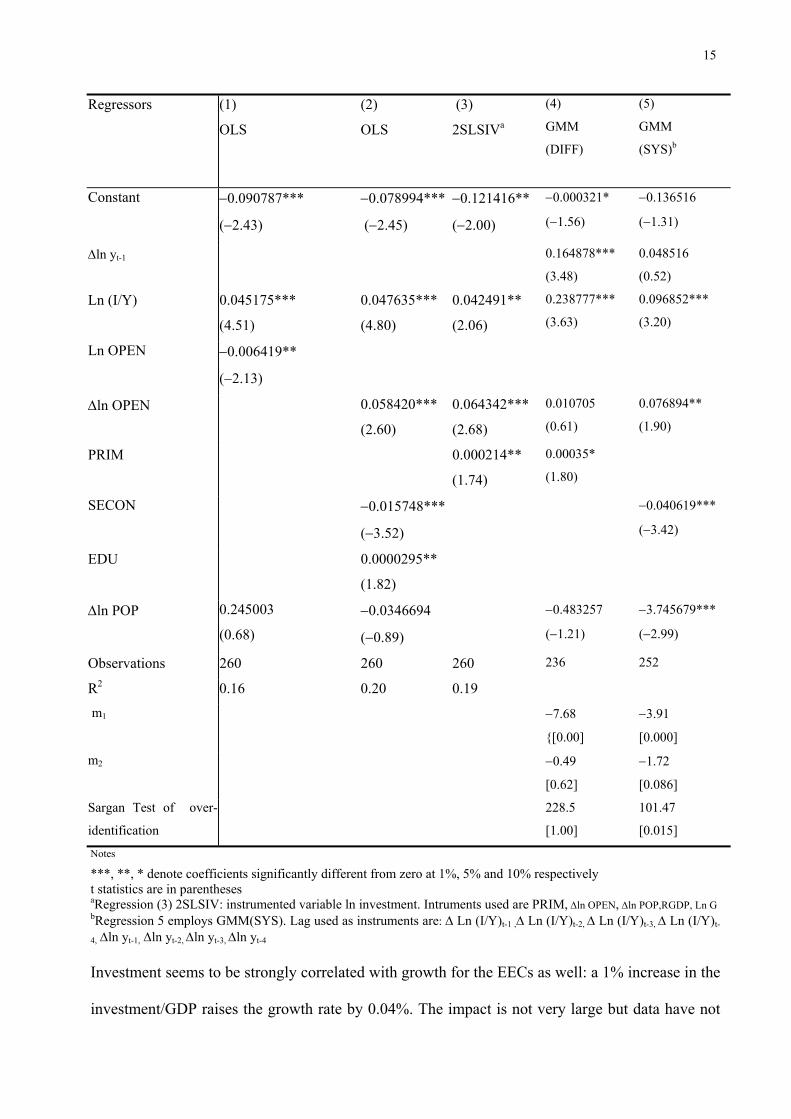
Table 3 Annual Data Cross-country Growth regression (1950-1990) EEC Sample. Dependent Variable ∆ln yt

15

Notes

***, **, * denote coefficients significantly different from zero at 1%, 5% and 10% respectively t statistics are in parentheses aRegression (3) 2SLSIV: instrumented variable ln investment. Intruments used are PRIM, ∆ln OPEN, ∆ln POP,RGDP, Ln G bRegression 5 employs GMM(SYS). Lag used as instruments are: ∆ Ln (I/Y)t-1 ,∆ Ln (I/Y)t-2, ∆ Ln (I/Y)t-3, ∆ Ln (I/Y)t-

4, ∆ln yt-1, ∆ln yt-2, ∆ln yt-3, ∆ln yt-4

Investment seems to be strongly correlated with growth for the EECs as well: a 1% increase in the

investment/GDP raises the growth rate by 0.04%. The impact is not very large but data have not

Regressors (1)

OLS

(2)

OLS

(3)

2SLSIVa

(4)

GMM

(DIFF)

(5)

GMM

(SYS)b

Constant −0.090787***

(−2.43)

−0.078994***

(−2.45)

−0.121416**

(−2.00)

−0.000321*

(−1.56)

−0.136516

(−1.31)

∆ln yt-1 0.164878***

(3.48)

0.048516

(0.52)

Ln (I/Y) 0.045175***

(4.51)

0.047635***

(4.80)

0.042491**

(2.06)

0.238777***

(3.63) 0.096852***

(3.20)

Ln OPEN −0.006419**

(−2.13)

∆ln OPEN 0.058420***

(2.60)

0.064342***

(2.68)

0.010705

(0.61) 0.076894**

(1.90)

PRIM 0.000214**

(1.74)

0.00035*

(1.80)

SECON −0.015748***

(−3.52)

−0.040619***

(−3.42)

EDU 0.0000295**

(1.82)

∆ln POP 0.245003

(0.68)

−0.0346694

(−0.89)

−0.483257

(−1.21)

−3.745679***

(−2.99)

Observations 260 260 260 236 252

R2 0.16 0.20 0.19 m1

−7.68

{[0.00]

−3.91

[0.000]

m2 −0.49

[0.62]

−1.72

[0.086]

Sargan Test of over-

identification

228.5

[1.00]

101.47

[0.015]

16

been transformed and the growth rate has not been multiplied by 100 as occurs generally in the

literature. As for CMEAs, openness in levels is robustly negatively correlated with growth

(regression 1). There are several ways to proceed from these unexpected negative results. The first

is to search for alternative proxies for openness. In some studies the growth rate of export or

import taken singularly have been used. We performed regressions with both measures in nominal

terms and the results were strongly positive for both. Obviously, negative coefficients were

obtained when the levels of both variables have been included in the same regression. As

explained openness in real terms, which takes into account both dimensions of access to foreign

market trade, is our preferred measure. There is another reason for the choice of openness as a

measure of trade intensity. Multivariate Dickey-Fuller test of the variables included in the

regressions showed that openness has a unit root and becomes stationary after first differencing

the variable while the same did not occur for the other measures reported in HS&A [2002]. As is

known this criticism applies to all empirical endogenous growth modelling that makes growth

rates a function of non-stationary variables. The inclusion of (log) differences in openness exhibits

a positive and robust coefficient in all the regressions based on annual data. Our result thus

suggest that when the proper measure of real openness is used it has a negative effect on growth

for EECs. This would indicate that the most empirical work that finds a strong and robust positive

result are either using different measures of trade policy or are likely to capture other

macroeconomic policies that are positively correlated with growth.

Concerning the other regressors, as for CMEAs, also for EECs the coefficient of primary

education is positive and significant. Also, we notice that interaction of primary education with

investment (EDU) has a positive impact on growth even if it is not large and the significance is

just at 10% level. The attempt to include other educational variables has not been satisfactory. The

negative coefficient of secondary education and average years of schooling on growth still remain

a puzzle in the empirics of growth (Wolff [2000])

17

The dynamic panel estimations (regressions 4 and 5) strengthen the previous findings. The

investment and the growth of openness variables have a strong impact on growth, although their

lagged values are statistically less significant. This might detect a strong cyclical effect of the

variables and a weak effect of the same variables on the long-run growth rates. Hence, we think

that the commonly used panel method which averages observations over five years should be

more reliable than yearly data to investigate long run effects of the same variables

Table 4: five-year period Regressions (1950-1990) EEC’s Sample

Dependent Variable: ∆ln yi,t

Regressors (1)

OLSDV

(2)

Fixed Effect (Within)

IVa

(3)

GMM (DIFF)b

(4)

GMM(SYS)

∆ln yt-1 0.543005***

(4.11)

0.480796***

(5.61)

0.564447***

(9.44)

0.275744**

(2.27)

Constant −0.59152

(−1.36)

−0.133493***

(−2.22)

−0.001395*

(−0.70)

-0.031648

(-0.99)

Ln (I/Y) 0.035529***

(3.04)

0.065221***

(4.41)

0.026512***

(2.36)

0.019784*

(1.93)

Ln OPEN −0.001535

(-0.44)

0.033202*

(1.64)

−0.011390

(−0.52)

0.003366

(0.82)

∆Ln POP 0.002329

(0.87)

Ln SECON −0.020647***

(−2.75)

0.004518

(0.50)

- 0.007259***

(-3.96)

SECON*OPEN −0.006889**

(−1.97)

0.003460

(0.88)

Ln AVERSCH −0.004692

(-0.65)

Ydum (1955-59) −0.003458

(−0.49)

Ydum (1960-64) −0.005839

(−0.81)

Ydum (1965-69) −0.003131

(−0.41)

18

Ydum (1970-74) −0.007681

(-1.04)

Ydum (1975-79) −0.008726

(−1.22)

dum (1980-84) −0.011051

(−1.46)

Ydum (1985-90) −0.011156*

(−1.58)

N. observations

R2

51

0.64

44

0.26

28 44

m1c -1.95

[0.051]

-1.91

[0.056}

m2 -0.20

[0.84]

0.40

[0.69]

HansenTest of over-

identifying restrictions

2.82

[1.00]

Notes.

***, **, * denote coefficients significantly different from zero at 1%, 5% and 10% respectively t statistics in parentheses and the p-value of the serial correlation tests are in square brackets aThe regression uses fixed effect within regression. The instrumented variable is Ln (I/Y; instruments are: all exogenous regressors + Ln (I/Y)t-1. bAdditional instruments used for the regressions are year dummies 1950-1990. Investment is treated as a potentially endogenous variable in GMM (DIFF) and GMM(SYS). The instrument set contains observations on all the variables in the equation dated t-2 and for GMM (SYS) the instruments used are the one in GMM(DIFF) + differences ∆ Ln (I/Y), ∆ Ln (I/Y) ∆ln OPEN dated t-1 c m1 and m2 are tests for first order and second order serial correlation in the first differenced residuals under the null of no serial correlation From table 4 we can observe that the only significant variable is investment in GDP. This is true

for all the methods used. However, when both lags of differences and lag of variables are used as

instruments, as in GMM(SYS), the investment looses part of its statistical significance. Human

capital continues to show a negative correlation with growth even when interaction terms are

introduced. In column 2 the interaction variable between openness and secondary education

(found generally positive in cross-country regression) exhibits a negative sign. The openness

variable does not seem to be a strong determinant of long run growth. In the endogenous growth

literature this variable has an indirect effect on growth trough the TFP. If international

specialisation of a country is oriented towards low technology goods the degree of openness can

be detrimental for productivity growth. In the case of EECs the result is at odds since we would

19

expect that TFP would be enhanced by economic integration between countries with high

standard of technologies, homogeneity in institutions, macroeconomic policy and market

structures.

4. Openness, trade structure and growth in transitional economies

The transition to market of former CMEAs has been associated with dramatic changes in

their foreign trade. Imports and exports have been strongly affected by processes of geographical

reorientation (especially towards the EU) and sectoral restructuring. In this section we try to

evaluate the relationship between openness and growth for a group of TEs14 in the period 1990-

2000).

Following Amable (2000), in addition to the openness measure, we consider as

explanatory variables some indices of sectoral composition of trade flows, such as inter-industry

index and dissimilarity index, in order to better qualify the link between trade and growth15. The

use of such trade structure indicators seems to us particularly appropriate for countries showing

relevant changes in the composition of their trade flows. In particular, such indices could signal if

inter or intra-specialisation promote growth in accordance with different models of trade

integration.

We complement inter-industry and dissimilarity measures with intra-industry indices

calculated at 8-digit level of disaggregation (at product level) . Such indices allow separating out

the share of trade flows differentiated by quality (vertical intra-industry trade) from the share of

trade flows differentiated by product attributes (horizontal intra-industry trade). This further

qualification of the trade flow structure is significant in order to disclose comparative advantage

dynamics operating inside both intra-industry (in the form of vertical intra-industry trade) and

inter-industry trade flows. If vertical component is the dominant part in intra-industry trade, then

14 We have considered 11 transitional economies: Hungary, Czech Republic, Slovakia, Poland, Bulgaria, Russia, Romania, Slovenia, Latvia, Estonia, Lithuania 15 Details on the construction of all trade indices used are in the appendix

20

trade could be better explained according to traditional arguments based on factor proportion and

differences in technology rather than theories based on imperfect competition. Hence, we

complement inter (intra)-industry indices calculated at 3-digit level with indices of vertical and

horizontal intra-industry trade calculated at 8-digit level. To better understand this point, compare

graph 1 and graph 2.

BGR

CZE

EST

HUNL TU

LVA

POL

ROMRUS

S VK

SVN

-.02

0.0

2.0

4av

erag

e gr

owth

(199

0-19

98)

.4 .6 .8inter-industry trade

grAVER Fitted v alues

Inter-industry trade and growth

BGR

CZE

EST

HUNLTU

LVA

POL

ROMRUS

SVK

SVN

-.02

0.0

2.0

4gr

owth

rat

e 19

90-1

998

.05 .1 .15 .2 .25 .3v ertical intra-industry trade (1990-1998)

grAVER Fitted v alues

vertical intra-industry trade and growth

Graph 1 displays a negative relationship between inter-industry trade and growth for the TEs in

the period 1990-98: more intra-industry trade (less inter-industry trade) is associated with more

growth. If we limited our observation to graph 1 in which inter (intra)-industry trade index has

been calculated at the 3-digit level, we would conclude that intra-industry specialisation promotes

growth and that the standard theory based on comparative advantages does not offer a good

prediction. But if we look at graph 2, in which trade index has been calculated at product level (8-

digit), we can observe that vertical intra-industry trade is positively associated with growth. In this

case, we cannot dismiss the traditional explanation based on comparative advantages because

vertical intra-industry is theoretically founded on a dynamics of specialisation based on factor

proportion (for example, different qualities incorporate different skill intensities).

Table 5 and table 6 describe results for the sample of TEs in the period 1990-2000. In

particular, table 5 reports regression results when trade indices at the 3-digit level are considered

as regressors, while table 6 shows results when trade indices at the 8-digit level are included.

21

Table 5. Trade and growth in transitional economies. Annual Data Cross-country Growth regression (1990-2000).

Dependent variable ∆ln yt. Trade indices at 3-digit level of disaggregation

Regressors (1)

OLS

(2)

OLS

(3)

OLS

(4)

OLS

Constant -0.1702129***

(-2.41)

-0.0163795

(-0.33)

-0.0320176

(-0.62)

0.0163638

(0.29)

Ln (I/Y) 0.0239028**

(1.95)

0.0268431**

(2.10)

0.0288855***

(2.23)

0.0283628***

(2.29)

∆Ln pop –0.4277895

(-0.86)

0.0179621

(0.04)

0.0407094

(0.09)

0.0671807

(0.15)

Ln OPEN 0.0250144**

(1.86)

INTER -0.086166**

(-1.89)

DISS(X) -0.0726609

(-1.37)

DISS(M) -0.262331***

(-2.26)

No. of Observ. 83 58 58 58

R2 0.08 0.17 0.15 0.19

Notes. ***, **, * denote coefficients significantly different from zero at 1%, 5% and 10% respectively t statistics in parenthesis

In the column (1) of table 5, the coefficient associated with openness is positive and

significant. This finding contrasts with previous results relative to CMEAs and supports the idea

of a positive influence of trade flows on growth when market mechanisms are in action. Columns

(2), (3) and (4) of table 5 show regression results when alternative measures of trade integration

are considered. In column (2), the inter-industry index is considered (INTER). This index has

been measured as the complement to one of the Grubel-Lloyd intra-industry trade index

calculated at the 3-digit level. The finding is that a negative and significant relationship emerges

between inter-industry trade and growth (at 5% level). However, as mentioned before, it is

important to investigate the type of intra-industry specialisation before inferring conclusions

about the model in action. In column (3), following Amable (2000), we consider as regressor the

dissimilarity index of exports. This index measures at to what extent the export composition by

sector of a transitional economy diverges from the export composition by sector of EU (value 1

22

indicates complete divergence, value 0 indicates complete convergence). The coefficient

associated with DISS(X) is negative but not significant. In column (4), we use the import

dissimilarity index. The coefficient associated with DISS(M) is negative and significant (at 1%

level). This should imply that a convergence towards the EU structure of demand for final goods

and input requirements promotes the growth of TEs. By looking at the other explanatory

variables, investment is significant in all specifications, thus confirming results obtained for

CMEAs and EECs.

In table 6 the coefficients of intra-industry trade indices are significant in almost all

specifications. In column (5), the Grubel-Lloyd intra-industry trade index calculated at 8-digit

level (GL) is positively associated with growth (at 5% level of significance). In column (6) and

(7) we can observe that both components of intra-industry trade – horizontal and vertical - are

positively related to growth (coefficients associated with GLH and GLV variables are significant

at 5% level). However, when we split the vertical intra-industry trade index in up-market (GLV+)

and down-market (GLV–) components, only the latter displays a significant coefficient. This

means that growth is positively related to specialisation in low quality goods.

In general, findings by using trade indices calculated at product level (8-digit) show that

both types of product differentiation dynamics, horizontal and vertical, have a positive influence

on growth. In such a case investment becomes insignificant. A likely explanation is that trade

indices, which signal product quality, should be better complemented by measures of human

capital rather than physical capital.

Table 6. Trade and growth in transitional economies. Annual Data Cross-country Growth regression (1990-2000).

Dependent variable ∆ln yt. Trade indices at 8-digit level of disaggregation

Regressors

(5)

OLS

(6)

OLS

(7)

OLS

(8)

OLS

(9)

OLS

23

Constant 0.083245

(0.04)

-0.072732**

(-1.85)

-0.08573**

(-2.14)

-0.081206**

(-2.01)

-0.08564**

(-2.14)

Ln (I/Y) 0.020747

(1.39)

0.018537

(1.22)

0.021809

(1.47)

0.0251768*

(1.71)

0.0217913

(1.47)

∆Ln pop 0.130432

(0.25)

-0.0041935

(-0.01)

0.1599507

(0.31)

0.1143399

(0.22)

0.1389768

(0.27)

GL 0.191316**

(1.92)

GLH 0.845921**

(2.00)

GLV 0.234801**

(1.85)

GLV+ 0.5074098

(1.44)

GLV– 0.319964**

(1.82)

Observ. 58 58 58 58 58

R2 0.16 0.16 0.15 0.13 0.15

Notes. ***, **, * denote coefficients significantly different from zero at 1%, 5% and 10% respectively t statistics in parentheses

5. Conclusions

This paper has investigated the relationship between trade-openness and growth. Overall,

our findings confirm that in planned economies the impact of openness defined in standard terms

is negative. But, surprisingly, the same variable has a strong negative effect also on the growth

rate of the EECs.

The finding of a negative correlation for the 2 major samples studied raises doubts about

the importance of this variable on long run growth performance. We started our work with the

expectation that openness should be influential for EEC but not for CMEA and realised that the

growth effects of openness, as measured by HS&A (2002), are not considerably different in both

samples. The only notable difference is that when we use the growth rate of openness, in the place

of its level, we find a positive relationship for the EECs but not for CMEAs. This result is found

using data at annual frequency. Regressions with five-year averages show, instead, a negative but

not significant coefficient for openness growth also for the EECs.

24

Although it is difficult to extract firm conclusions from the analysis above, what is

perhaps most notable from our regressions is that all different econometric methods used show the

same negative impact of the trade variable on growth.

The paper also provides findings regarding the robustness of other growth determinants:

(i) only investment in physical capital is strongly correlated with growth in the two historical

samples, (ii) standard measures of human capital are negatively correlated with growth, except for

primary education in both samples, but not in all the specifications.

The robustness of the investment share is not startling if we think that Levine and Renelt

(1992) achieved similar conclusions more than ten years ago by applying the extreme bound

analysis to cross-section regressions. Also for CMEA, investment has been the most important

growth determinant as deliberately stated by the policy agenda of the Communist Party.

Regarding the trade-growth relationship the most substantive result is that for EEC

openness is important when annual data are considered and this should explain short-run effects

more than long-run growth. This argument is supported by results obtained from the third sample

considered. In TEs the time period is too short to infer long run effects of trade on growth. In fact,

results reveal a substantial role of openness during the transition. Motivated by the fact that the

integration measure is rightly signed we have constructed indices of inter-industry and intra-

industry trade for this panel of countries. Openness and intra-industry trade indices seem to be

significant determinants of their growth transitional path. However, when we split the vertical

intra-industry trade index in up-market (GLV+) and down-market (GLV–) components, only the

latter displays a significant coefficient.

Should we infer that trade does spur growth particularly at the beginning of the process of

opening up to international integration, the subsequent effects being unable to sustain accelerating

growth processes, as witnessed by empirical and historical experience of EEC? A likely

explanation is that there might be diminishing returns for a very large trade share. But another

25

equally likely hypothesis is that the standard measure of openness adopted is not adequate to

capture the effects of trade in the EEC.

References Aghion, P. and Howitt, P.(1992), A Model of Growth through Creative Destruction, Econometrica , 60, 423-351 Alcalà , F. Ciccone, A. (2004) Trade and Productivity, Quarterly Journal of Economics, 119, 613-646

Amable, B. (2000), International specialisation and Growth, Structural Change and Economic Dynamics, 11, 413-431 Arellano, M. and Bond, S.R. (1991) Some tests of Specification for Panel Data: Monte Carlo Evidence and an Application

to Employment Equations, Review of Economic Studies, 58, 277-297 Arellano, M. and Bover, O. (1995) Another Look at the Instrumental Variable Estimation of Error Component, Journal of

Econometrics, 68, 29-52 Barro, R. and Jong-Wha Lee (1993) International Comparison of Educational Attainments, Journal of Monetary

Economics 32, dec. 363-394 Barro, R. and Jong-Wha Lee (2000), International Data on Educational Attainment: Updates and Implications, NBER

Working Paper, N. 7911 (web site for data from the Center for International Development at Harvard University: www.cid.harvard.edu/ciddata.html)

Barro, R. and Sala-i-Martin, X. (1995) Economic Growth, McGraw Hill, New York Benhabib, J. and Spiegel, M. (1994) The role of Human Capital in Economic Development: Evidence from Aggregate

Cross-Country Data, Journal of Monetary Economics, 34, 143-173 Benhabib, J. and Spiegel, M. (2000) The Role of Financial Development in Growth and Investment, Journal of Economic

Growth, 5, 341-360 Benhabib, J. and Spiegel, M. (2002) Human capital and Technology Diffusion, forthcoming in Handbook of Economic

Growth, North-Holland. Blundell, R. and Bover, S (1998) Initial Condition and Moment Restrictions in Dynamic Panel Data Model, Journal of

Econometrics, 87, 115-143 Bond S.R. Hoeffler, A. and Temple, J. (2001) GMM Estimation of Empirical Growth Models, CEPR Discussion Paper, n.

3048 Caselli F., Esquivel G. and Lefort F (1996). Reopening the Convergence debate: A New Look at Cross Country Growth

Empirics, Journal of Economic Growth, 1, 363-389 Dollar, D. and Kraay, A. (2003) Institutions, Trade and growth, Journal of Monetary Economics, 50, 133-162 Edwards, S. (1993) Openness, Trade Liberalisation, and Growth in Developing Countries, Journal of Economic

Literature, 31, 1358-393 Edwards, S. (1998), Openness, Productivity and Growth: What We Really Know? The Economic Journal, 108, 383-398 Frankel, J. and Romer, D (1999) Does trade cause Growth? American Economic Review, 89, 373-399 Grier, R. (2002) On the Interaction of Human and Physical Capital in Latin America, Economic Development and

Cultural Change, pp. 891-913 Grossman, G.M. and Helpman, E. (1991) Innovation and Growth in a Global Economy, MIT Press, Cambridge Harrison, A. (1996), Openness and Growth: A Time Series, Cross-Country Analysis for Developing Countries, Journal of

Development Economics, 48, 419-447. Henrekson, M.Torstensson J. and Torstensson R. (1997) Growth Effects of European Integration, European Economic

Review, 41, 1537-1557 Heston, A., Summers, R and Aten, B (2002) The Penn World Table (Mark 6.1), http: www.nber.org Irwin, D. and Tervio, M (2002) Does Trade Raise Income? Evidence from the Twentieth Century, Journal of

International Economics, 58, 1-18 Klenow, P.J. and Rodriguez-Clare, A. (1999) The Neoclassical Revival in Growth Economics: Has It Gone Too Far? in

NBER Macroeconomic Annual, 73-103 Lavigne, M. (1995) The Economics of Transition: From Socialist Economy to Market Economy. St Martin Press, New

York Lee H.Y., Ricci, L.A. and Rogobon R. (2004) Once Again, Is Openness Good for Growth?, NBER Working Paper No.

10749 Levine, R. and Renelt, D. (1992) A Sensitive Analysis of cross-country Growth Regressions, American Economic Review,

82, sept. 942-963

26

Mankiw, N.G., Romer, D. and Weil, N.D. (1992) A Contribute to the Empirics of Economic Growth Quarterly Journal of Economics, 107, May 407-437

Matsuyama, K (1992), Agricoltural Productivity, Comparative Advantage, and economic Growth, Journal of Economic Theory, 58, 317-34

Miller, S. M., Upadhayay, M.P. (2000), The Effects of Openness, Trade Orientation, and Human Capital on Total Factor Productivity, Journal of Development Economics, 63, 399-423

Pritchett, L. (2001) Where Has All the Education Gone?, The World Bank Economic Review, 15, 367-391 Psacharopoulos , G. (1994) Returns to Investment in Education: A Global Update, World Development , 22, 1325-1343 Rivera –Batiz F. and Romer P.M. (1991), Economic Integration and Economic Growth, Quarterly Journal of Economics,

106, 531-555 Rodriguez and Rodrick, D. (1999) Trade Policy and Economic Growth, NBER Working Paper No. 7081, April Rodrick, D, Subramanian A. and Trebbi F (2002) Institutions Rule: The primacy over Geography and Interaction in

Economic Development, NBER WP, No. 9305 Sachs, J. And Warner, A. (1995), Economic Reform and The process of Global Integration, Brookings Papers on

Economic Activity, August , 1-118 Sachs, J. And Warner, A.(2001) Fundamental Sources of Long Run Growth, American Economic Review, Paper and

Proceedings, 87, 184-188 Scheets N. and Boata, S. (1996) Eastern European Export Performance During the Transition, Board of Governors of the

Federal Reserve System, International Finance Discussion paper, N. 562 Schrenk, M. (1992) CMEA Trade and Payments: Conditions for Institutional Change, in B. Milanovic and Hillman

(editors) The Transition from Socialism in Eastern Europe: Domestic Restructuring and Foreign Trade. World Bank Summers, R. and Heston, A. (1991) The Penn World Table (Mark 5): An Expanded set of International Comparison

1950-1988, Quarterly Journal of Economics, may, 327-368 Vamvakidis, A. (2002) How Robust is the Growth-Openness Connection? Historical Evidence, Journal of Economic

Growth, 7, 57-80 Wacziarg and Welch (2003) Integration and Growth: An Update, NBER Working Paper, n. 10152, December Wacziarc R. (2001) Measuring the Dynamic Gains from Growth, The World Bank Economic Review. 15, 393-343 Wolff, E.N. (2000) Human capital Investment and Economic Growth: Exploring the Cross-country Evidence, Structural

Change and Economic Dynamic, 11, 433-472 Appendix

Samples

We use three samples. The first one is composed by EEC countries: Belgium, France, West Germany, Italy,

Netherlands (data are from 1950) United Kingdom, Ireland and Denmark (data are included from 1970)

The second sample is formed by historically planned economies (CMEAs) which includes: Czechoslovakia, Poland,

Hungary, Bulgaria, Romania, East Germany (DDR), USSR and Yugoslavia. In earlier version of PWT only 3 of these

countries were included in the data set (Hungary, Poland and Yugoslavia). All the countries participated in the 1996

benchmark comparisons carried out through the OECD and have been treated individually by [2002]. Estimates of

components of GDP and related variables for these countries are subject to some measurement errors. To signal the

relative reliability of the estimates, the authors have assigned to the data quality of these countries a rating scale

between B and C against a rating scale of A which is assigned to all the countries in the EEC panel (see Table A of

[2002, p. 13 Data Appendix of Penn World table 6.1).

The third sample is formed by ex-CMEA and accession countries: Hungary, Czech Republic, Slovakia, Poland,

Bulgaria, Russia, Romania, Slovenia, Latvia, Estonia, Lithuania.

List of Variables

POP: population is from the World Bank World Development Indicators 2001 and United Nations Development

centre for sources prior to 1960.

RGDPxx : real GDP per capita (1995 international prices) for 19xx ( RGDPCH in 2002

INVxx : investment share of RGDP (KI in 2002)

27

OPENxx (KOPEN in [2002]) is the ratio of export plus imports in exchange rate US $ relative to GDP in PPP (US$

PPP/GDP)

GOV xx: Government share of RGDP (KG in 2002).

Trade indices

INTER: inter-industry trade index calculated as 1 – GL index,

∑

∑∑∑∑

+

−−+=

+

−−=

i ii

i iii ii

i ii

i iij MX

MXMXMXMX

GL)(

)()(

1 ,

where j= country, i=3-digit industry, X=exports, M=imports

DISS(X)j = export dissimilarity index = ∑ −eu

ieu

j

ij

XX

XX

2/1

where eu= EU

DISS(M)j = import dissimilarity index = ∑ −eu

ieu

j

ij

MM

MM

2/1

GLHj = horizontal intra-industry trade index = ∑

∑∑+

−−+∈∈

p pp

Hp ppHp pp

MX

MXMX

)(

)(

where p= 8-digit product, UVp are the unit values of exports (x) and imports (m), α = 0.15 and the summation p∈H in the numerator is over those 8-digit commodities for which

αα +≤≤− 11 mp

xp

UVUV

,

GLVj = vertical intra-industry trade index = ∑∑∑+

−−+∈∈

p pp

Vp ppVp pp

MX

MXMX

)(

)(

ωηερε τηε συµµατιον π∈ς ισ οϖερ τηοσε 8�διγιτ χοµµοδιτιεσ φορ ωηιχη

αα +≥−≤ 1or 1 mp

xp

mp

xp

UVUV

UVUV

GLVj+ = up-market vertical intra-industry trade index = ∑

∑∑+

−−+∈∈

p pp

Up ppUp pp

MX

MXMX

)(

)(

where the summation p∈U is over those 8-digit commodities for which α+≥ 1mp

xp

UVUV

28

GLVj– = down-market vertical intra-ind. trade index = ∑

∑∑+

−−+∈∈

p pp

Dp ppDp pp

MX

MXMX

)(

)(

where the summation p∈D is over those 8-digit commodities for which 1 α−≤mp

xp

UVUV

Since the sets V and H are mutually exclusive and exhaustive and since the sets U and D are mutually exclusive and exhaustive of V, it follows immediately that

−+−

++= GLVGLVGLHGLdigitj )8(

Data Sources

Data for the main variables listed above are from Heston, Summers and Aten (2002), Penn World Tables, version .6.1

Data for human capital (PRIM, SECON, AVERAGE) are taken from Barro and Lee (1993) and updated from Barro

and Lee (2000). PRIM (LP in Barro and Lee [2000] is the percentage of primary school attained in the total

population. SECON is the” percentage of secondary school attained” in the total population (LS in Barro and Lee

[2000] and AVERAGE is the average schooling years in the total population (PYR in Barro and Lee [2000])

EDUxx has been used to interact human capital with openness or investment. The precise meaning of the variables is

given in the notes to each regression (it is the natural logarithm of the percentage of different degrees of schooling

attained in the total population aged 25 and above in 19xx multiplied by the natural log of the investment share or

openness share).

Trade data for the TEs are taken from the EUROSTAT COMEXT database. From this database, we have considered

135 3-digit sectors classified according to NACE-CLIO and 13724 8-digit products classified according Combined

Nomenclature.