online appendix mobilizing the masses for genocide
TRANSCRIPT

Online AppendixMobilizing the Masses for Genocide
Thorsten Rogall
A.1 Additional Tables and Figures
A.2 Extensions to Section II. – Data
A.3 Extensions to Section III. – Understanding theFirst Stage
A.4 Extensions to Section III. – Placebo, ExclusionRestriction, and Robustness Checks
A.5 Extensions to Section V. – Network Effects
A.6 Extensions to Section VI. – Information, Mate-rial Incentives, and Retaliation
A.7 Extensions to Section VI. – Modeling the Forceversus Obedience Channel
A.8 Proofs
A.1

A.1 Additional Tables and Figures
Table A.1: Clustered Standard Errors
Dependent Variable: # Militiamen, log # Civilian Perpetrators, log
First Stage Reduced Form OLS IV/2SLS
(1) (2) (3) (4)
Distance × Rainfall along Buffer, 1994 −0.509 −0.661Clustered, Commune Level (0.144) (0.162)Clustered, District Level (0.144) (0.162)Clustered, Province Level (0.118) (0.171)Bootstrap, District 0.006 0.002Bootstrap, Province 0.002 0.002
# Militiamen, log 0.626 1.299(0.039) (0.244)(0.047) (0.291)(0.069) (0.236)0.000 0.0010.000 0.011
Standard Controls yes yes yes yesGrowing Season Controls yes yes yes yesAdditional Controls yes yes yes yesProvince Effects yes yes yes yes
R2 0.50 0.58 0.74 .N 1432 1432 1432 1432
Notes: The first standard errors reported under each coefficient are clustered at the commune level, the second clusteredat the district level, the third at the province level. The fourth and fifth entry under each coefficient are p-values using awild bootstrap to account for the small number of district/province clusters. Distance × Rainfall along Buffer, 1994 isthe instrument (distance to the main road interacted with rainfall along the way between village and main road during the100 days of the genocide in 1994). Standard Controls include village population, distance to the main road, rainfall inthe village during the 100 days of the genocide in 1994, long-term average rainfall in the village during the 100 calenderdays of the genocide period (average for 1984-1993), rainfall along the buffer during the 100 days of the genocide in1994, long-term average rainfall along the buffer during the 100 calender days of the genocide period (1984-1993), andthe latter interacted with distance to the main road. Growing Season Controls are rainfall during the growing seasonin 1994 in the village, 10 year long-term average rainfall during the growing seasons in the village and both of theseinteracted with the difference between the maximum distance to the road in the sample and the actual distance to theroad. Additional Controls are distance to Kigali, main city, borders, Nyanza (old Tutsi Kingdom capital) as well aspopulation density in 1991 and the number of days with RPF presence. All control variables, except “Number of Dayswith RPF presence,” are in logs. Interactions are first logged and then interacted. In each column I also control for maineffects and double interactions. There are 142 communes, 30 districts, and 11 provinces in the sample.
A.2
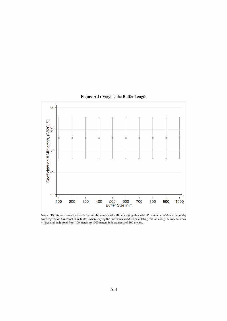
Figure A.1: Varying the Buffer Length
Notes: The figure shows the coefficient on the number of militiamen (together with 95 percent confidence intervals)from regression 6 in Panel B in Table 3 when varying the buffer size used for calculating rainfall along the way betweenvillage and main road from 100 meters to 1000 meters in increments of 100 meters.
A.3
Tabl
eA
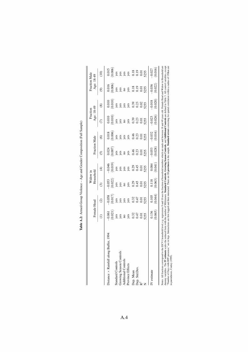
.2:A
rmed
-Gro
upV
iole
nce
–A
gean
dG
ende
rCom
posi
tion
(Ful
lSam
ple)
Wid
owin
Frac
tion
Frac
tion
Mal
eFe
mal
eH
ead
Hou
seho
ldFr
actio
nM
ale
Age
:18-
49A
ge:1
8-49
(1)
(2)
(3)
(4)
(5)
(6)
(7)
(8)
(9)
(10)
Dis
tanc
e×
Rai
nfal
lalo
ngB
uffe
r,19
94−
0.06
1−
0.05
8−
0.05
3−
0.04
60.
024
0.01
80.
010
0.01
00.
016
0.01
5(0
.021)
(0.0
17)
(0.0
22)
(0.0
19)
(0.0
07)
(0.0
06)
(0.0
10)
(0.0
10)
(0.0
06)
(0.0
06)
Stan
dard
Con
trol
sye
sye
sye
sye
sye
sye
sye
sye
sye
sye
sG
row
ing
Seas
onC
ontr
ols
yes
yes
yes
yes
yes
yes
yes
yes
yes
yes
Add
ition
alC
ontr
ols
noye
sno
yes
noye
sno
yes
noye
sPr
ovin
ceE
ffec
tsye
sye
sye
sye
sye
sye
sye
sye
sye
sye
s
Dep
.Mea
n0.
320.
320.
290.
290.
460.
460.
390.
390.
180.
18D
ep.S
td.D
ev.
0.47
0.47
0.45
0.45
0.23
0.23
0.23
0.23
0.19
0.19
R2
0.01
0.01
0.01
0.01
0.01
0.01
0.01
0.02
0.01
0.01
N52
5552
5552
5552
5552
5552
5552
5552
5552
5552
55
IVes
timat
e0.
136
0.10
50.
118
0.08
4−
0.05
3−
0.03
2−
0.02
3−
0.01
8−
0.03
6−
0.02
7(0
.065)
(0.0
44)
(0.0
63)
(0.0
41)
(0.0
28)
(0.0
16)
(0.0
26)
(0.0
20)
(0.0
22)
(0.0
16)
Not
es:A
llfr
actio
nsco
rres
pond
toth
eE
ICV
1ho
useh
old
leve
l,e.
g.re
gres
sion
s9
and
10us
eth
efr
actio
nof
hous
ehol
dm
embe
rsw
hich
are
mal
ean
dbe
twee
n18
and
49ye
ars
old.
Fem
ale
Hea
dan
dW
idow
inH
ouse
hold
are
dum
my
vari
able
s.T
heIV
estim
ate
scal
esth
ere
duce
dfo
rmw
ithth
enu
mbe
rofM
ilitia
men
.Sta
ndar
dC
ontr
ols,
Gro
win
gSe
ason
Con
trol
s,an
dA
dditi
onal
Con
trol
sare
defin
edin
Tabl
e3.
All
cont
rolv
aria
bles
,exc
ept
“Num
bero
fDay
sw
ithR
PFpr
esen
ce,”
are
inlo
gs.I
nter
actio
nsar
efir
stlo
gged
and
then
inte
ract
ed.T
here
are
11pr
ovin
cesi
nth
esa
mpl
e.St
anda
rder
rors
corr
ectin
gfo
rspa
tialc
orre
latio
nw
ithin
ara
dius
of15
0km
are
inpa
rent
hese
s,C
onle
y(1
999)
.
A.4

Tabl
eA
.3:L
ocal
Vio
lenc
e–
Age
and
Gen
derC
ompo
sitio
n(F
ullS
ampl
e)
Frac
tion
Frac
tion
Mal
eW
idow
inA
ge:1
3-49
Age
:13-
49Fe
mal
eH
ead
Hou
seho
ldFr
actio
nM
ale
(1)
(2)
(3)
(4)
(5)
(6)
(7)
(8)
(9)
(10)
Rad
ioC
over
age
inV
illag
e0.
109
0.11
20.
106
0.10
7−
0.03
0−
0.05
1−
0.03
4−
0.05
10.
055
0.06
1(0
.033)
(0.0
33)
(0.0
53)
(0.0
49)
(0.1
45)
(0.1
26)
(0.1
16)
(0.0
97)
(0.0
60)
(0.0
51)
Prop
agat
ion
Con
trol
sye
sye
sye
sye
sye
sye
sye
sye
sye
sye
sA
dditi
onal
Con
trol
sno
yes
noye
sno
yes
noye
sno
yes
Com
mun
eE
ffec
tsye
sye
sye
sye
sye
sye
sye
sye
sye
sye
s
Dep
.Mea
n0.
530.
530.
240.
240.
320.
320.
300.
300.
460.
46D
ep.S
td.D
ev.
0.23
0.23
0.21
0.21
0.47
0.47
0.46
0.46
0.23
0.23
R2
0.07
0.07
0.05
0.05
0.05
0.06
0.05
0.05
0.04
0.04
N40
3940
3940
3940
3940
3940
3940
3940
3940
3940
39
IVes
timat
e0.
216
0.21
90.
210
0.20
8−
0.06
0−
0.09
9−
0.06
8−
0.10
00.
109
0.11
9(0
.266)
(0.2
86)
(0.2
41)
(0.2
63)
(0.2
75)
(0.2
69)
(0.2
41)
(0.2
47)
(0.1
39)
(0.1
56)
Not
es:A
llfr
actio
nsco
rres
pond
toth
eE
ICV
1ho
useh
old
leve
l,e.
g.re
gres
sion
s3
and
4us
eth
efr
actio
nof
hous
ehol
dm
embe
rsw
hich
are
mal
ean
dbe
twee
n13
and
49ye
ars
old.
Fem
ale
Hea
dan
dW
idow
inH
ouse
hold
are
dum
my
vari
able
s.T
heIV
estim
ate
scal
esth
ere
duce
dfo
rmw
ithth
enu
mbe
rof
Mili
tiam
en.
Prop
agat
ion
cont
rols
are:
latit
ude,
long
itude
,ase
cond
orde
rpo
lyno
mia
lin
villa
gem
ean
altit
ude,
villa
geal
titud
eva
rian
ce,
and
ase
cond
orde
rpo
lyno
mia
lin
the
dist
ance
toth
ene
ares
ttra
nsm
itter
.A
dditi
onal
Con
trol
sin
clud
edi
stan
ceto
the
road
,dis
tanc
eto
the
bord
er,d
ista
nce
tom
ajor
city
,pop
ulat
ion
and
popu
latio
nde
nsity
,and
slop
ing
dum
mie
s.T
here
are
128
com
mun
esin
the
sam
ple.
Stan
dard
erro
rsin
pare
nthe
ses
are
clus
tere
dat
dist
rict
leve
l.
A.5

Tabl
eA
.4:A
rmed
-Gro
upV
iole
nce
–C
ompl
iers
I
Dep
ende
ntV
aria
ble:
#M
ilitia
men
,log
Sam
ple:
Popu
latio
nD
ensi
tyR
ain-
fed
Prod
uctio
nC
apita
lCity
RPF
Pres
ence
Hig
hL
owH
igh
Low
Far
Clo
seL
ong
Shor
t
(1)
(2)
(3)
(4)
(5)
(6)
(7)
(8)
Dis
tanc
e×
Rai
nfal
lalo
ngB
uffe
r,19
94−
0.31
4−
0.50
7−
0.43
8−
0.71
4−
0.29
4−
0.65
3−
0.48
5−
0.32
3(0
.086)
(0.2
38)
(0.1
73)
(0.1
58)
(0.2
11)
(0.0
78)
(0.1
22)
(0.1
83)
Stan
dard
Con
trol
sye
sye
sye
sye
sye
sye
sye
sye
sG
row
ing
Seas
onC
ontr
ols
yes
yes
yes
yes
yes
yes
yes
yes
Add
ition
alC
ontr
ols
yes
yes
yes
yes
yes
yes
yes
yes
Prov
ince
Eff
ects
yes
yes
yes
yes
yes
yes
yes
yes
R2
0.56
0.48
0.47
0.56
0.46
0.63
0.63
0.35
N71
671
671
671
671
671
665
977
3
Not
es:
The
sam
ples
are
defin
edin
the
colu
mn
head
ings
.T
hefu
llsa
mpl
eis
split
atth
em
edia
nfo
rth
eva
riab
les
popu
latio
nde
nsity
inre
gres
sion
s1
and
2,lo
ng-t
erm
rain
fall
duri
ngth
egr
owin
gse
ason
sin
the
villa
gein
regr
essi
ons
3an
d4,
dist
ance
toth
eca
pita
lKig
alii
nre
gres
sion
s5
and
6an
dfin
ally
num
bero
fday
sw
ithR
PFpr
esen
cein
regr
essi
ons7
and
8.St
anda
rdC
ontr
olsi
nclu
devi
llage
popu
latio
n,di
stan
ceto
the
mai
nro
ad,r
ainf
alli
nth
evi
llage
duri
ngth
e10
0da
ysof
the
geno
cide
in19
94,l
ong-
term
aver
age
rain
fall
inth
evi
llage
duri
ngth
e10
0ca
lend
erda
ysof
the
geno
cide
peri
od(a
vera
gefo
r198
4-19
93),
rain
fall
alon
gth
ebu
ffer
duri
ngth
e10
0da
ysof
the
geno
cide
in19
94,l
ong-
term
aver
age
rain
fall
alon
gth
ebu
ffer
duri
ngth
e10
0ca
lend
erda
ysof
the
geno
cide
peri
od(1
984-
1993
),an
dth
ela
tteri
nter
acte
dw
ithdi
stan
ceto
the
mai
nro
ad.G
row
ing
Seas
onC
ontr
olsa
rera
infa
lldu
ring
the
grow
ing
seas
onin
1994
inth
evi
llage
,10
year
long
-ter
mav
erag
era
infa
lldu
ring
the
grow
ing
seas
ons
inth
evi
llage
and
both
ofth
ese
inte
ract
edw
ithth
edi
ffer
ence
betw
een
the
max
imum
dist
ance
toth
ero
adin
the
sam
ple
and
the
actu
aldi
stan
ceto
the
road
.Add
ition
alC
ontr
olsa
redi
stan
ceto
Kig
ali,
mai
nci
ty,b
orde
rs,N
yanz
a(o
ldTu
tsiK
ingd
omca
pita
l)as
wel
las
popu
latio
nde
nsity
in19
91an
dth
enu
mbe
rof
days
with
RPF
pres
ence
.A
llco
ntro
lva
riab
les,
exce
pt“N
umbe
rof
Day
sw
ithR
PFpr
esen
ce,”
are
inlo
gs.
Inte
ract
ions
are
first
logg
edan
dth
enin
tera
cted
.T
here
are
11pr
ovin
ces
inth
esa
mpl
e.St
anda
rder
rors
corr
ectin
gfo
rspa
tialc
orre
latio
nw
ithin
ara
dius
of15
0km
are
inpa
rent
hese
s,C
onle
y(1
999)
.
A.6

Tabl
eA
.5:L
ocal
Vio
lenc
e–
Com
plie
rsI
Dep
ende
ntV
aria
ble:
#M
ilitia
men
,log
Sam
ple:
Popu
latio
nD
ensi
tyR
ain-
fed
Prod
uctio
nC
apita
lCity
RPF
Pres
ence
Hig
hL
owH
igh
Low
Far
Clo
seL
ong
Shor
t
(1)
(2)
(3)
(4)
(5)
(6)
(7)
(8)
Rad
ioC
over
age
inV
illag
e0.
552
0.62
30.
430
0.78
40.
578
0.21
60.
587
0.32
1(0
.278)
(0.6
08)
(0.2
04)
(0.4
69)
(0.2
13)
(0.4
11)
(0.4
28)
(0.1
81)
Prop
agat
ion
Con
trol
sye
sye
sye
sye
sye
sye
sye
sye
sA
dditi
onal
Con
trol
sye
sye
sye
sye
sye
sye
sye
sye
sC
omm
une
Eff
ects
yes
yes
yes
yes
yes
yes
yes
yes
R2
0.60
0.58
0.51
0.66
0.48
0.69
0.69
0.47
N52
852
952
852
952
852
951
154
6
Not
es:
The
sam
ples
are
defin
edin
the
colu
mn
head
ings
.T
hefu
llsa
mpl
eis
split
atth
em
edia
nfo
rthe
vari
able
spo
pula
tion
dens
ityin
regr
essi
ons1
and
2,lo
ng-t
erm
rain
fall
duri
ngth
egr
owin
gse
ason
sin
the
villa
gein
regr
essi
ons3
and
4,di
stan
ceto
the
capi
talK
igal
iin
regr
essi
ons
5an
d6
and
final
lynu
mbe
rof
days
with
RPF
pres
ence
inre
gres
sion
s7
and
8.Pr
opag
atio
nC
ontr
ols
are:
latit
ude,
long
itude
,ase
cond
orde
rpol
ynom
iali
nvi
llage
mea
nal
titud
e,vi
llage
altit
ude
vari
ance
,and
ase
cond
orde
rpol
ynom
iali
nth
edi
stan
ceto
the
near
estt
rans
mitt
er.A
dditi
onal
Con
trol
sinc
lude
dist
ance
toth
ero
ad,d
ista
nce
toth
ebo
rder
,dis
tanc
eto
maj
orci
ty,p
opul
atio
nan
dpo
pula
tion
dens
ity,
and
slop
ing
dum
mie
s.T
here
are
128
com
mun
esin
the
full
sam
ple.
Stan
dard
erro
rsin
pare
nthe
ses
are
clus
tere
dat
dist
rict
leve
l.
A.7

Tabl
eA
.6:A
rmed
-Gro
upV
iole
nce
–C
ompl
iers
II
Dep
ende
ntV
aria
ble:
#M
ilitia
men
,log
Sam
ple:
Mal
eH
HFr
actio
n13
-49
Frac
tion
Mal
e,13
-49
Frac
tion
18-4
9Fr
actio
nM
ale,
18-4
9H
igh
Low
Hig
hL
owH
igh
Low
Hig
hL
owH
igh
Low
(1)
(2)
(3)
(4)
(5)
(6)
(7)
(8)
(9)
(10)
Dis
tanc
e×
Rai
nfal
lalo
ngB
uffe
r,19
94−
0.32
5−
0.54
9−
0.28
4−
0.56
8−
0.27
6−
0.67
2−
0.36
6−
0.54
0−
0.26
7−
0.63
7(0
.132)
(0.0
92)
(0.1
63)
(0.1
49)
(0.1
58)
(0.2
12)
(0.1
73)
(0.1
75)
(0.1
57)
(0.2
04)
Stan
dard
Con
trol
sye
sye
sye
sye
sye
sye
sye
sye
sye
sye
sG
row
ing
Seas
onC
ontr
ols
yes
yes
yes
yes
yes
yes
yes
yes
yes
yes
Add
ition
alC
ontr
ols
yes
yes
yes
yes
yes
yes
yes
yes
yes
yes
Prov
ince
Eff
ects
yes
yes
yes
yes
yes
yes
yes
yes
yes
yes
R2
0.44
0.60
0.43
0.50
0.42
0.52
0.38
0.53
0.38
0.53
N71
571
771
172
171
571
771
371
970
872
4
Not
es:
The
sam
ples
are
defin
edin
the
colu
mn
head
ings
.T
hefu
llsa
mpl
eis
split
atth
em
edia
nfo
rth
efr
actio
nof
hous
ehol
dsw
itha
mal
ehe
adin
regr
essi
ons
1an
d2,
the
aver
age
frac
tion
ofho
useh
old
mem
bers
aged
13to
49in
regr
essi
ons
3an
d4,
the
aver
age
frac
tion
ofm
ale
hous
ehol
dm
embe
rsag
ed13
to49
inre
gres
sion
s5
and
6an
dfin
ally
the
sam
eas
befo
rew
itha
diff
eren
tage
cuto
ff(1
8to
49)
inre
gres
sion
s7
to10
.St
anda
rdC
ontr
ols
incl
ude
villa
gepo
pula
tion,
dist
ance
toth
em
ain
road
,ra
infa
llin
the
villa
gedu
ring
the
100
days
ofth
ege
noci
dein
1994
,lon
g-te
rmav
erag
era
infa
llin
the
villa
gedu
ring
the
100
cale
nder
days
ofth
ege
noci
depe
riod
(ave
rage
for
1984
-199
3),r
ainf
alla
long
the
buff
erdu
ring
the
100
days
ofth
ege
noci
dein
1994
,lon
g-te
rmav
erag
era
infa
llal
ong
the
buff
erdu
ring
the
100
cale
nder
days
ofth
ege
noci
depe
riod
(198
4-19
93),
and
the
latte
rin
tera
cted
with
dist
ance
toth
em
ain
road
.G
row
ing
Seas
onC
ontr
ols
are
rain
fall
duri
ngth
egr
owin
gse
ason
in19
94in
the
villa
ge,1
0ye
arlo
ng-t
erm
aver
age
rain
fall
duri
ngth
egr
owin
gse
ason
sin
the
villa
gean
dbo
thof
thes
ein
tera
cted
with
the
diff
eren
cebe
twee
nth
em
axim
umdi
stan
ceto
the
road
inth
esa
mpl
ean
dth
eac
tual
dist
ance
toth
ero
ad.A
dditi
onal
Con
trol
sare
dist
ance
toK
igal
i,m
ain
city
,bor
ders
,Nya
nza
(old
Tuts
iKin
gdom
capi
tal)
asw
ella
spo
pula
tion
dens
ityin
1991
and
the
num
ber
ofda
ysw
ithR
PFpr
esen
ce.
All
cont
rolv
aria
bles
,exc
ept“
Num
ber
ofD
ays
with
RPF
pres
ence
,”ar
ein
logs
.In
tera
ctio
nsar
efir
stlo
gged
and
then
inte
ract
ed.
The
rear
e11
prov
ince
sin
the
sam
ple.
Stan
dard
erro
rsco
rrec
ting
for
spat
ialc
orre
latio
nw
ithin
ara
dius
of15
0km
are
inpa
rent
hese
s,C
onle
y(1
999)
.
A.8
Tabl
eA
.7:L
ocal
Vio
lenc
e–
Com
plie
rsII
Dep
ende
ntV
aria
ble:
#M
ilitia
men
,log
Sam
ple:
Mal
eH
HFr
actio
n13
-49
Frac
tion
Mal
e,13
-49
Frac
tion
18-4
9Fr
actio
nM
ale,
18-4
9H
igh
Low
Hig
hL
owH
igh
Low
Hig
hL
owH
igh
Low
(1)
(2)
(3)
(4)
(5)
(6)
(7)
(8)
(9)
(10)
Rad
ioC
over
age
inV
illag
e0.
382
0.94
20.
343
0.60
10.
380
0.60
30.
435
0.55
50.
351
0.62
3(0
.322)
(0.3
74)
(0.3
85)
(0.3
19)
(0.4
02)
(0.2
54)
(0.3
86)
(0.3
11)
(0.3
93)
(0.2
50)
Prop
agat
ion
Con
trol
sye
sye
sye
sye
sye
sye
sye
sye
sye
sye
sA
dditi
onal
Con
trol
sye
sye
sye
sye
sye
sye
sye
sye
sye
sye
sC
omm
une
Eff
ects
yes
yes
yes
yes
yes
yes
yes
yes
yes
yes
R2
0.56
0.63
0.38
0.58
0.42
0.58
0.39
0.58
0.41
0.59
N52
553
252
852
952
053
752
253
552
852
9
Not
es:
The
sam
ples
are
defin
edin
the
colu
mn
head
ings
.T
hefu
llsa
mpl
eis
split
atth
em
edia
nfo
rth
efr
actio
nof
hous
ehol
dsw
itha
mal
ehe
adin
regr
essi
ons1
and
2,th
eav
erag
efr
actio
nof
hous
ehol
dm
embe
rsag
ed13
to49
inre
gres
sion
s3an
d4,
the
aver
age
frac
tion
ofm
ale
hous
ehol
dm
embe
rsag
ed13
to49
inre
gres
sion
s5an
d6
and
final
lyth
esa
me
asbe
fore
with
adi
ffer
enta
gecu
toff
(18
to49
)in
regr
essi
ons7
to10
.Pro
paga
tion
Con
trol
sar
e:la
titud
e,lo
ngitu
de,a
seco
ndor
der
poly
nom
iali
nvi
llage
mea
nal
titud
e,vi
llage
altit
ude
vari
ance
,and
ase
cond
orde
rpo
lyno
mia
lin
the
dist
ance
toth
ene
ares
ttra
nsm
itter
.A
dditi
onal
Con
trol
sin
clud
edi
stan
ceto
the
road
,dis
tanc
eto
the
bord
er,d
ista
nce
tom
ajor
city
,pop
ulat
ion
and
popu
latio
nde
nsity
,and
slop
ing
dum
mie
s.T
here
are
128
com
mun
esin
the
full
sam
ple.
Stan
dard
erro
rsin
pare
nthe
ses
are
clus
tere
dat
dist
rict
leve
l.
A.9
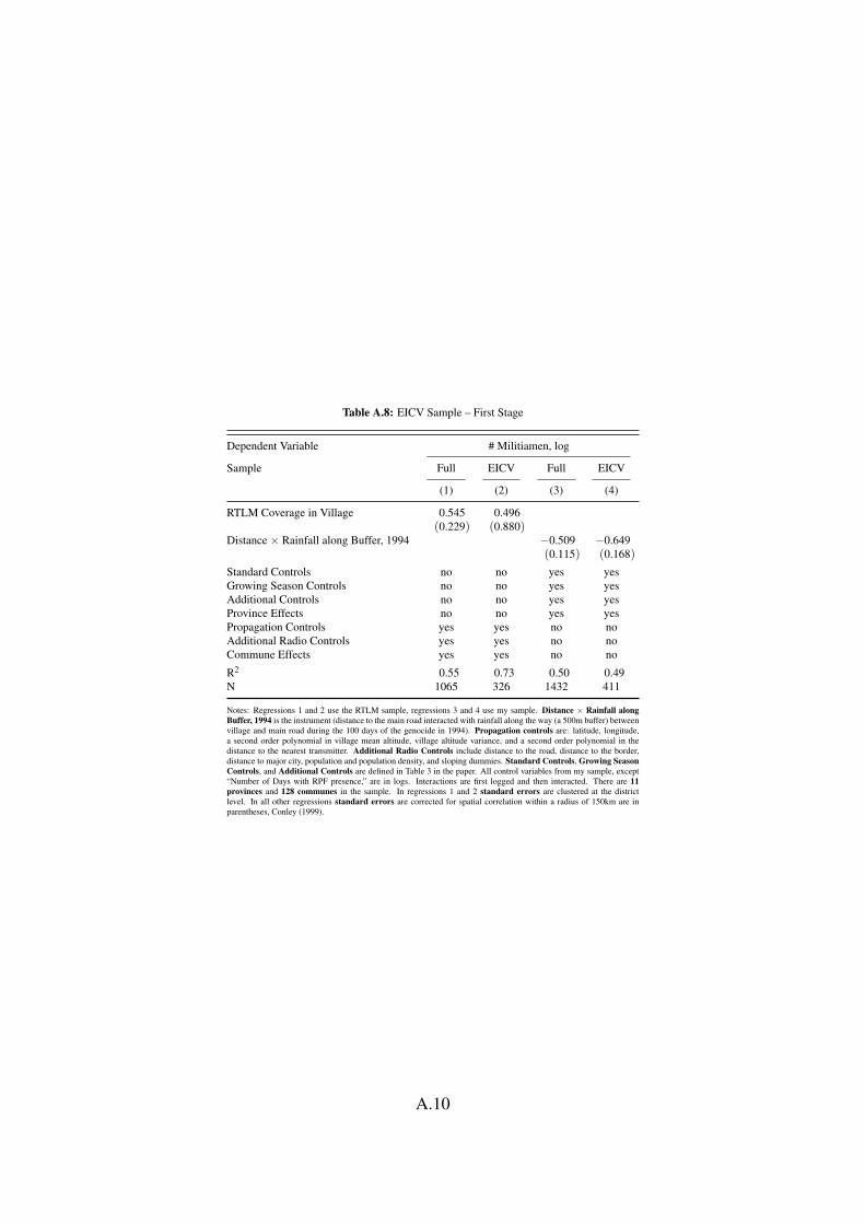
Table A.8: EICV Sample – First Stage
Dependent Variable # Militiamen, log
Sample Full EICV Full EICV
(1) (2) (3) (4)
RTLM Coverage in Village 0.545 0.496(0.229) (0.880)
Distance × Rainfall along Buffer, 1994 −0.509 −0.649(0.115) (0.168)
Standard Controls no no yes yesGrowing Season Controls no no yes yesAdditional Controls no no yes yesProvince Effects no no yes yesPropagation Controls yes yes no noAdditional Radio Controls yes yes no noCommune Effects yes yes no no
R2 0.55 0.73 0.50 0.49N 1065 326 1432 411
Notes: Regressions 1 and 2 use the RTLM sample, regressions 3 and 4 use my sample. Distance × Rainfall alongBuffer, 1994 is the instrument (distance to the main road interacted with rainfall along the way (a 500m buffer) betweenvillage and main road during the 100 days of the genocide in 1994). Propagation controls are: latitude, longitude,a second order polynomial in village mean altitude, village altitude variance, and a second order polynomial in thedistance to the nearest transmitter. Additional Radio Controls include distance to the road, distance to the border,distance to major city, population and population density, and sloping dummies. Standard Controls, Growing SeasonControls, and Additional Controls are defined in Table 3 in the paper. All control variables from my sample, except“Number of Days with RPF presence,” are in logs. Interactions are first logged and then interacted. There are 11provinces and 128 communes in the sample. In regressions 1 and 2 standard errors are clustered at the districtlevel. In all other regressions standard errors are corrected for spatial correlation within a radius of 150km are inparentheses, Conley (1999).
A.10

A.2 Extensions to Section II. – Data
A.2.1 Data Matching
I combine several datasets from different sources to construct the final dataset,which comprises 1,433 Rwandan villages. The different datasets are matchedby village names within communes.1 Unfortunately, the matching is imperfect,as some villages either have different names in different data sources, or usemultiple spellings. However, overall only about 5 percent of the villages donot have a clear match across all sources. Furthermore, these issues are likelyidiosyncratic, resulting in less precise estimates.
A.2.2 Participation in Violence
The two key measures are participation in armed-group violence and partici-pation in civilian violence. Since no direct measure of participation is avail-able, I use prosecution numbers for crimes committed during the genocide as aproxy. Importantly, individuals were prosecuted in the village where they com-mitted the crime (individuals did not have to be present in that village to beprosecuted). Depending on the role played by the accused, two categories ofcriminals are identified by the courts.
Category 1 includes perpetrators that mostly belong to the army and themilitia or are members of local armed groups such as policemen, thus I con-sider this to represent armed-group violence. There were approximately 77,000prosecution cases in this category (Figure A.2). Note that this number does notnecessarily equal the number of people involved. Consistent with organizedperpetrators moving around, there are cases where people were prosecuted inmultiple locations. Since external militiamen were thus likely prosecuted in ab-sence they could not have simply accused civilians to positively affect their ownverdict. The legal definition of category 1 includes: 1) planners, organizers, in-stigators, supervisors of the genocide; 2) leaders at the national, provincial ordistrict level, within political parties, army, religious denominations or militia;3) the well-known murderer who distinguished himself because of the zeal thatcharacterized him in the killings or the excessive wickedness with which killings
1A commune is an administrative unit above the village. There were 142 communes in total,which were in turn grouped into 11 provinces.
A.11
were carried out; and 4) people who committed rape or acts of sexual torture.The legal definition for category 1 also comprises rapists and torturers who
may have been civilians. However, civilians being falsely classified as militi-amen in the data, would only work against my findings and bias the estimatesdownwards.2 Besides, anecdotal evidence suggests that the especially gruesomeand cruel killings (including sexual violence and rape) were in fact committedby militia members. The vast majority of civilian killers did not seem to sadis-tically enjoy the killings (Hatzfeld, 2005).
People accused in category 2 are not members of any of the organized groupsmentioned in category 1 and I therefore label this category civilian violence.Approximately 430,000 prosecution cases were handled in this category (Fig-ure A.3). The legal definition of category 2 includes: 1) authors, co-authors,accomplices of deliberate homicides, or of serious attacks that caused some-one’s death; 2) the person who – with the intention of killing – caused injuriesor committed other serious acts of violence, but without actually causing death;and 3) the person who committed criminal acts or became the accomplice ofserious attacks, without the intention of causing death.
The reliability of the prosecution data is a key issue for the analysis. In lightof the chaos in the aftermath of the genocide, one might wonder about the gen-eral quality of the Gacaca data. Reassuringly, the Gacaca courts have been verythorough in investigating the various prosecution cases, taking about six yearsto complete their work (the first courts were set up in 2001).3 Besides, sincemuch of the violence was highly localized people knew the perpetrators welland could easily identify them later on in the prosecution process. Friedman(2010, p. 21) notes that “reports of those afraid to speak are rare, so this data
is likely to be a good proxy for the number of participants in each area.” Andeven identifying external militiamen was possible because they wore distinctiveuniforms indicating their area of origin (Des Forges, 1999). “A survivor of that
massacre identified the party affiliation of the assailants from their distinctive
garb, the blue and yellow print boubou of the Interahamwe and the black, yel-
2Reducing the number of militiamen and increasing the number of civilians in the data ro-tates the first-stage line counterclockwise and the reduced-form line clockwise, which implieslarger instrumental-variables estimates. Naturally, villages with many prosecuted militiamenwere, if at all, more likely to have some falsely classified civilians.
3As an aside, note that the courts’ actions (starting in 2001) are therefore unlikely to becorrelated with the instrument which uses rainfall from 1994.
A.12
low, and red neckerchiefs and hats of the Impuzamugambi. He could tell, too,
that they came from several regions.” Des Forges (1999, p. 180). Thus aftercross-checking these accusations with other villages, the local courts were ableto also prosecute external perpetrators.
As a first reliability test of the data, Friedman (2010) shows that the Gacacadata is positively correlated with several other measures of violence from threedifferent sources.4 Nevertheless, some measurement error may always exist butwould only matter as much as it is correlated with the instrument. In particular,random measurement error and allegations that these courts were occasionallymisused to settle old scores, resulting in false accusations do not pose any majorthreat because I am instrumenting for armed-group violence.
However, non-classical measurement error may matter. One potentially im-portant case is the presence of survival bias: in those villages with high partici-pation, the violence might have been so widespread that no witnesses were leftto accuse the perpetrators, resulting in low prosecution rates. Another concernis that villages with no reported armed-group violence might have actually re-ceived militiamen, but unsuccessful ones. To ease all these concerns that somesystematic, non-classical measurement error is biasing the results, I will presentseveral additional tests in the following section.
A.2.3 Reliability of the Gacaca Data
In this section, I perform a number of tests to ease concerns that measurementerror leads to any systematic biases (random measurement error does not posea threat). As noted above, one potentially important case is the presence of sur-vival bias: in those villages with high participation, the violence might havebeen so widespread that no witnesses were left to accuse the perpetrators, re-sulting in low prosecution rates. This would be particularly worrisome if it hap-pened in places that were potentially landlocked due to heavy rains and peoplecould not flee.
In general, large transport costs were unlikely to hinder the Tutsi from es-caping, since they avoided the main roads as road blocks were set up throughoutthe country (Hatzfeld, 2005). Thus, their movements should not be correlated
4These sources are a database from Davenport and Stam (2009), the PRIO/Uppsala data(Gleditsch et al., 2002), and a report from the Ministry of Higher Education (Kapiteni, 1996).
A.13
with the instrument. If anything they should have been more likely to flee ifthe road had been blocked preventing the militia to arrive – however this wouldonly work against my findings. To nevertheless ease the concern of survivalbias, I show that the results are robust to using several alternative measures ofgenocide violence, in particular actual death data which does not suffer from thesame prosecution reporting bias.
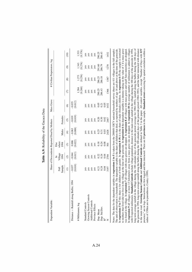
Child Mortality As a first alternative genocide violence outcome, I use childmortality data from the Rwandan EICV household survey from 2000/01 intro-duced above. The dependent variable is the share of children in the householdthat died, as reported by mothers of age 16 and above at the time of the genocide.Note that there is no age restriction on children – thus, depending on the age ofthe mother, some of the children are adults themselves.5 Regression 1 in TableA.9 shows that the instrument indeed negatively maps into child mortality. Re-assuringly, child mortality is only affected for individuals that experienced thegenocide in their village (regression 2). For individuals that only later moved totheir surveyed location the effect is small and insignificant (regression 3). Fur-thermore, consistent with the armed-group violence targeted especially at males,these negative effects seem to be driven by male mortality (regressions 4 and 5).
Regarding magnitude, the point estimate of -0.063 (standard error 0.008)for males suggests that a village with an average distance to the main road hasabout 15 percent lower male mortality rates, following a one standard-deviationincrease in rainfall between village and main road. This effect is very similar tothe ones obtained using the Gacaca prosecution data (for militiamen this numberranges between 20 and 30 percent).6
Deaths at Commune Level As another alternative outcome variable for geno-cide violence, I use data on Tutsi death estimates at the commune level. Unfortu-nately, this data is not available for my whole sample of villages. Nevertheless,regressions 1 to 3 in Table A.11 show that armed groups’ transport costs neg-
5Results are robust to varying the mother cutoff age (regressions 1 to 5 in Table A.10).6These results are also robust to controlling for average rainfall (years 1995 to 2001) during
the 100 calendar days of the genocide period along the way between village and main road andits interaction with distance to the main road. Recall that the survey data is from 2001, thusrainfall between 1995 and 2001 may be a confounder. Results can be found in regressions 6 to10 in Table A.10.
A.14

atively map into Tutsi deaths (since the data is only available at the communelevel I simply assume that each village (within a given commune) receives anequal share of deaths). In regressions 4 to 6, I then rerun the analysis at thecommune level. Although the number of observations drop significantly, armedgroups’ transport costs is still strongly negatively related to the number of Tutsideaths. The data on the commune-level death estimates is provided by Genody-namics. These estimates are generated using a Bayesian latent variable model oninformation from five different sources: the Ministry of Education in Rwanda,the Ministry of Local Affairs in Rwanda, Ibuka (the Rwandan survivor organi-zation), African Rights, and Human Rights Watch.7
DHS Data Sibling Deaths As yet another outcome variable, I use data fromthe three latest DHS Rounds (2005, 2010 and 2015). All three rounds containa question on how many years ago an individual’s sibling died (NISR et al.,2016, 2012; INSR et al., 2006). First, I show that 1994 is a clear outlier in thedistribution of deaths, around 25 percent of all reported deaths happened in thatyear. The average for all other years is about 3.7 percent (Figure A.4). Second,I show that my instrument is negatively related to the number of deaths onlyfor 1994 (in all three rounds). For all other years, the point estimate on the in-strument oscillates around zero (Figure A.5). Note that the effects for 1994 getslightly weaker over time (i.e. the different DHS rounds), this is unsurprisingsince migration is likely to create measurement error and bias the point esti-mate downwards (unfortunately, the DHS data for Rwanda does not allow me toidentify whether an individual experienced the genocide in the survey location).The results not only confirm that my instrument has a strong effect on genocidedeaths but also show that it does not have an effect on other deaths.
Mass Graves Moreover, recall from the discussion on RTLM violence abovethat the militia’s transport costs also negatively map into whether a mass gravesite was found in the village (I re-report the regression in column 6 in Table A.9).The point estimate of -0.035 suggests that a village with an average distance tothe main road is 37 percent less likely to have a mass grave site, given a onestandard-deviation increase in rainfall between village and main road (recall themagnitudes for armed-group violence from the Gacaca data: 20 to 30 percent).
7For more details see: https://genodynamics.weebly.com.
A.15

Besides, by dropping those villages with mass grave sites (i.e. villages withhigh death rates) and rerunning the baseline regression, I provide another testfor ruling out the presence of potential survival bias in the prosecution data.Importantly, the instrumental-variables point estimates are virtually identical tothe baseline results and similarly significant at the 99 percent confidence level(regression 7). Since especially small Tutsi minorities might have been at riskof being completely wiped out (and thus unable to identify the perpetrators),in the next regression I only drop villages with both a mass grave site and asmall Tutsi minority. Again, the results are very similar to the baseline numbers(regression 8). Finally, the results are also robust to dropping villages less than3.5 kilometers away from a mass grave location, reducing the sample size byabout 10 percent (regression 9).
Underreporting Next, potential underreporting of unsuccessful militiamen,something that would bias the OLS estimates upwards, is unlikely to push up theinstrumental-variables estimates as well. To see this, I add the average numberof militiamen per village in the sample to those villages with zero militiamenreported (only those with a Tutsi minority) and rerun the baseline regression.The point estimate of 1.533 (standard error 0.376, regression 10) is very similarto the baseline results and if anything higher. This is unsurprising, since the re-duced form is unaffected by this change and the first-stage coefficient decreasesin absolute terms.8 As a result the instrumental-variables estimates should in-crease.9
Migration Bias Another concern, besides survival bias, is potential migrationbias. Towards the end of the genocide several hundreds of thousands Hutu fledRwanda in fear of the RPF’s revenge. If people’s decision to flee is correlated
8Adding militiamen to low-violence villages, that is villages that were hard to reach, rotatesthe first-stage regression line counterclockwise.
9Besides, it seems puzzling that a genocide planner who wants to maximize civilian partici-pation and the number of Tutsi deaths, would send ineffective militiamen specifically to villagesthat are hard to reach: not only are the (wasted) costs of getting there higher but the monitor-ing costs will certainly be higher as well. Moreover, I am not aware of any anecdotal evidencesupporting the notion of lazy or unsuccessful militiamen. If anything, the contrary seems to betrue: in Hatzfeld (2005, p. 10), a civilian killer reports that the militiamen were the “younghotheads” who ragged the others on the killing job. Another one continues (p. 62), “When theInterahamwe noticed idlers, that could be serious. They would shout, We came a long way togive you a hand, and you’re slopping around behind the papyrus!”
A.16

with the instrument this might bias the results. This is particularly true if inplaces that are harder to reach by the militia and subsequently by the RPF, Hutucivilians are more likely to succeed in escaping. Although individuals were alsoprosecuted in abstenia it might still be the case that prosecutors who had escapedwere not well-known (especially civilians) and thus forgotten.
Note that prosecution in absentia did happen in around 15 percent of thecases (de Brouwer and Ruvebena (2013)). One of the reasons for this wasthat the Gacaca courts, besides bringing perpetrators to justice, also tried toacknowledge the suffering of the victims. Thus discussing a case in the ab-sence of the accused was part of the post-genocide reconciliation effort (Ny-seht Brehm (2014)). In several cases though did perpetrators return and pleadguilty (this would often lead to a reduction in their sentence). Detailed migra-tion data from the Rwandan EICV household survey in 2000/01 (representativeat national level) suggests that around 81 percent of the refugees returning toRwanda moved back into their home village (and only 19 percent choose a newlocation). This is consistent with a number of studies suggesting that even aftermajor conflict episodes, such as those in Sierra Leone or Rwanda, individualtend to move back to their homelands (Glennerster et al., 2013; UN, 1996).On a side note, the large majority – around 90 to 92 percent – of the sampledindividuals in 2000/01 experienced the genocide in their surveyed location.
I present a number of results suggesting that migration is unlikely to bias myeffects. First, the large majority of Hutu (and Tutsi) fled Rwanda towards theend of the genocide. Thus transport costs at the beginning of the genocide (onceI control for costs towards the end) are unlikely to suffer from the same bias.In Table A.15 below, I show that my results are robust to using only rainfallfor the first 5 days, first week or first 2 weeks in the excluded instrument whilecontrolling for the remaining genocide days. Second, the RPF from which theHutu were fleeing took over Rwanda gradually. It is thus unlikely that theirmovements are correlated with the instrument. In regressions 5 and 6 in TableA.12, I regress the number of days each village was under RPF control on theinstrument. The point estimates are small and insignificant.
Finally, I can use detailed migration data from the Rwandan EICV house-hold survey in 2000/01 to shed light on migration patterns.
I first identify refugees who fled Rwanda during the genocide and then re-turned to their home village afterwards. In regression 1 in Panel A. in Table
A.17
A.12, I show that being a refugee is uncorrelated with the instrument. Oneobvious caveat is that I only observe people who returned (e.g. survived) inmy sample. However, once people escaped, the decision to return (after thegenocide) is unlikely correlated with the instrument (using rainfall during thegenocide). Besides, those refugees escaping from high cost villages were morelikely to survive since the RPF could not reach them. Thus, if anything, the truerelationship between transport costs and being a refugee should be negative andthus go against my findings.
For completeness, I can also show that the instrument is uncorrelated withwhether an individual was internally displaced. Note that is this case I am testingwhether low transport costs increased chances that an individual would moveinto a given village. Again, I do not expect their decisions to escape, facingdeath, to be the result of a rational transport cost calculation, as was the case forthe militia. Consistently, the effect is small and insignificant (regression 2).
Furthermore, the results are robust to splitting the sample by gender andfocusing only on adult males (regressions 1 to 6 in Panel B. in Table A.12).
A.2.4 Rainfall Data
I use the recently released National Oceanic and Atmospheric Administration(NOAA, 2010) database of daily rainfall estimates for Africa, which stretchesback to 1983, as a source of exogenous weather variation (Novella and Thiaw,2012).10 The NOAA data relies on a combination of weather station data as wellas satellite information to derive rainfall estimates at 0.1 degree (∼ 11 km at theequator) latitude longitude intervals. Considering the small size of Rwanda,this high spatial resolution data is crucial to obtain reasonable rainfall variation.Furthermore, the high temporal resolution, i.e. daily estimates, allows me toconfine variation in rainfall in the instrument to the exact period of the genocide.
To construct the instrument, I compute the amount of rainfall during the pe-riod of the genocide over a 500-meter buffer around the distance line betweeneach village centroid and the closest point on the main road (Figure A.6 below il-lustrates this).11 Since these buffers crisscross the various rainfall grids and each
10ftp://ftp.cpc.ncep.noaa.gov/fews/fewsdata/africa/arc2/bin/.11Taking the village centroid to calculate distances is standard practice and furthermore very
reasonable for Rwanda with its very high population density (apart from the few nature reserves– which are excluded – there is no uninhabited space in Rwanda).
A.18

distance buffer is thus likely to overlap with more than one rainfall grid, I obtainconsiderable variation in rainfall along each buffer.12 Furthermore, Rwanda’shilly terrain ensures sufficient local variation in rainfall (micro-climates), i.e theclouds get stuck somewhere and it rains on one side of the mountain but not onthe other. The overall rainfall in each buffer is obtained through a weighted av-erage of the grids, where the weights are given by the relative areas covered byeach grid.13 In a similar fashion, using a village boundary map, I also computerainfall in each village.
A.2.5 Village Map and Africover Data
The Center for Geographic Information Systems and Remote Sensing of the Na-tional University of Rwanda (CGIS-NUR) in Butare provides a village boundarymap, importantly with additional information on both recent and old adminis-trative groupings (Verpoorten, 2012). Since Rwandan villages have been re-grouped under different higher administrative units a number of times after thegenocide, this information allows me to match villages across different datasets(e.g. the 1991 census and the Gacaca records).
Africover (2002a, 2002b) provides maps with the location of major roadsand cities derived from satellite imagery. These satellites analyze light andother reflected materials, and any emitted radiation from the surface of the earth.Since simple dirt roads have different radiation signatures than tarred roads orgravel roads, this allows to objectively measure road quality.14
References
[1] Africover. 2002a. “Roads of Rwanda –12In some cases multiple rainfall buffers fall within the same single rainfall grid. However,
this only happens for about 9 percent of the villages. The location of these villages is shown inFigure A.7 below. Naturally, this happens for villages very close to the main roads.
13Figure A.8 maps the variation in the difference between rainfall along each buffer duringthe genocide in 1994 and its long-term average (years 1984-1993) for each village.
14Because the satellite pictures are taken a little after the genocide, towards the middle andend of the 1990s, I also cross-check the data with a Rwandan road map from 1994. Except forone road, which runs south of Kigali, all roads match. That missing road, however, was of badquality and only upgraded sometime after 2000. Consequently, the satellites did not detect it.The results become weaker when including that road which is reasonable given the measurementerror it creates.
A.19

AFRICOVER.” Provided by FAO GeoNetwork athttp://rkp.review.fao.org/geonetwork/srv/api/records/7970dfcf-99eb-414b-a5d1-4d028c17454b (accessed 2011).
[2] Africover. 2002b. “Towns of Rwanda –AFRICOVER.” Provided by FAO GeoNetwork athttp://rkp.review.fao.org/geonetwork/srv/api/records/661929d8-4219-450c-a343-3ec421699226 (accessed 2011).
[3] de Brouwer A.M. and E. Ruvebana. 2013. The Legacy of the GacacaCourts in Rwanda: Survivors’ Views. International Criminal Law Review,13(5): 937-976.
[4] Des Forges, A. 1999. Leave None to Tell the Story: Genocide in Rwanda,New York: Human Rights Watch.
[5] Friedman, W. 2010. Local Economic Condi-tions and Participation in the Rwandan Genocide,http://cega.berkeley.edu/assets/miscellaneous files/wgape/19 Friedman.pdf.
[6] Gleditsch, N. P., Wallensteen, P., Eriksson, M., Sollenberg, M. and H.Strand. 2002. Armed conflict 1946-2001: A new dataset, Journal of Peace
Research, 39(5): 615-637.
[7] Glennerster, R., Miguel, E., and A. Rothenberg. 2013. Collective Actionin Diverse Sierra Leone Communities. Economic Journal, 123(568): 285-316.
[8] Hatzfeld, J. 2005. Machete season: The Killers in Rwanda speak, NewYork: Picador.
[9] Institut National de la Statistique du Rwanda - INSR and ORC Macro.2006. Rwanda Demographic and Health Survey 2005, Calverton, Maryland,USA: INSR and ORC Macro. https://dhsprogram.com/data/ (accessed Jan-uary 2018).
[10] Kapiteni, A. 1996. La premiere estimation du hombre des victims dugenocide du Rwanda de 1994 commune par commune en Fev. 1996, Re-port of the Ministry of Higher Education, Scientific Research, and Culture.http://rwanda.free.fr/docs1 c.htm
A.20

[11] National Institute of Statistics of Rwanda - NISR, Ministry of Health- MOH/Rwanda, and ICF International. 2012. Rwanda Demographicand Health Survey 2010, Calverton, Maryland, USA: NISR/Rwanda,MOH/Rwanda, and ICF International. https://dhsprogram.com/data/ (ac-cessed January 2018).
[12] National Institute of Statistics of Rwanda - NISR, Ministry of Financeand Economic Planning/Rwanda, Ministry of Health/Rwanda, and ICFInternational. 2016. Rwanda Demographic and Health Survey 2014-15,Kigali, Rwanda: National Institute of Statistics of Rwanda, Ministry of Fi-nance and Economic Planning/Rwanda, Ministry of Health/Rwanda, andICF International. https://dhsprogram.com/data/ (accessed January 2018).
[13] National Oceanic and Atmospheric Administration (NOAA).2010. African Rainfall Climatology from the Famine Early Warn-ing System. In cooperation with National Centers for Environ-mental Prediction (NCEP) and Climate Prediction Center (CPC),ftp://ftp.cpc.ncep.noaa.gov/fews/fewsdata/africa/arc2/bin/
[14] Novella, Nicholas S., and Wassila M. Thiaw (2012). African RainfallClimatology Version 2 for Famine Early Warning Systems. Journal of Ap-
plied Meteorology and Climatology, 52(3): 588-606.
[15] Nyseth Brehm H., Uggen C., and J.D. Gasanabo. Genocide, Justice,and Rwanda’s Gacaca Courts. Journal of Contemporary Criminal Justice,30(3): 333-352.
[16] Verpoorten, M. 2012. “Command- and Datafile for the Replicationof: Detecting Hidden Violence: The Spatial Distribution of ExcessMortality in Rwanda. (2012). Political Geography. 31(1): 44-56.”https://www.uantwerpen.be/en/staff/marijkeverpoorten/my-website/data/(accessed 2014, Rwandan sector shape file requested and received directlyfrom the author).
[17] United Nations (UN). 1996. General Assembly - Situation in Rwanda: in-ternational assistance for a solution to the problems of refugees,the restora-tion of total peace, reconstruction and socio-economic development inRwanda. Report of the Secretary-General, A/51/353
A.21
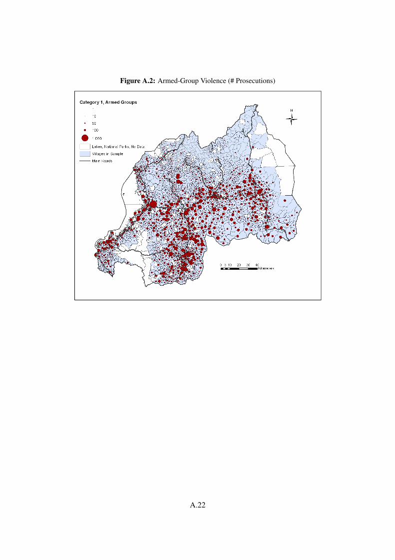
Figure A.2: Armed-Group Violence (# Prosecutions)
A.22

Figure A.3: Civilian Violence (# Prosecutions)
A.23
Tabl
eA
.9:R
elia
bilit
yof
the
Gac
aca
Dat
a
Dep
ende
ntV
aria
ble:
Shar
eof
Des
cend
ents
Rep
orte
dD
ead
byM
othe
rsM
ass
Gra
ve#
Civ
ilian
Perp
etra
tors
,log
InE
lse
Full
Vill
age
whe
reSa
mpl
e19
9419
94M
ales
Fem
ales
(1)
(2)
(3)
(4)
(5)
(6)
(7)
(8)
(9)
(10)
Dis
tanc
e×
Rai
nfal
lalo
ngB
uffe
r,19
94−
0.03
7−
0.04
40.
006
−0.
063
−0.
019
−0.
035
(0.0
10)
(0.0
13)
(0.0
22)
(0.0
08)
(0.0
19)
(0.0
12)
#M
ilitia
men
,log
1.28
41.
273
1.34
31.
533
(0.2
68)
(0.2
56)
(0.2
76)
(0.3
76)
Stan
dard
Con
trol
sye
sye
sye
sye
sye
sye
sye
sye
sye
sye
sG
row
ing
Seas
onC
ontr
ols
yes
yes
yes
yes
yes
yes
yes
yes
yes
yes
Add
ition
alC
ontr
ols
yes
yes
yes
yes
yes
yes
yes
yes
yes
yes
Prov
ince
Eff
ects
yes
yes
yes
yes
yes
yes
yes
yes
yes
yes
Dep
.Mea
n0.
210.
220.
180.
250.
200.
0529
0.25
286.
2529
1.60
290.
25D
ep.S
td.D
ev.
0.24
0.24
0.24
0.31
0.30
0.21
286.
4328
6.18
286.
7928
6.43
R2
0.04
0.04
0.08
0.03
0.02
0.05
..
..
N31
9727
0450
124
2824
6714
3213
6613
8712
7014
32
Not
es:
The
data
for
the
depe
nden
tvar
iabl
esin
regr
essi
ons
1to
5is
take
nfr
omth
e20
00/0
1E
ICV
natio
nalh
ouse
hold
surv
ey(t
here
are
411
villa
ges
inth
efu
llsa
mpl
e).
The
unit
ofob
serv
atio
nis
aho
useh
old.
The
depe
nden
tvar
iabl
eis
the
shar
eof
child
ren
that
died
,as
repo
rted
bym
othe
rsof
age
16an
dab
ove
atth
etim
eof
the
geno
cide
.In
regr
essi
ons
5to
7th
issh
are
isfo
rch
ildre
nof
both
gend
er.
Inre
gres
sion
8(9
)iti
sth
esh
are
ofm
ale
(fem
ale)
child
ren.
Inre
gres
sion
6(7
)the
sam
ple
isre
stri
cted
tom
othe
rsth
atliv
ed(d
idno
tliv
e)in
the
villa
geat
the
time
ofth
ege
noci
de.
Inre
gres
sion
6th
ede
pend
entv
aria
ble
isa
dum
my
taki
ngon
the
valu
eof
1if
am
ass
grav
ew
asfo
und
inth
evi
llage
.In
regr
essi
on7
allv
illag
esw
ithm
ass
grav
esar
edr
oppe
d.In
regr
essi
on8
allv
illag
esw
ithm
ass
grav
esan
dsm
allT
utsi
min
oriti
esar
edr
oppe
d.In
regr
essi
on9
allv
illag
esat
mos
t3.5
kilo
met
ers
away
from
am
ass
grav
esi
tear
edr
oppe
d.In
regr
essi
on10
the
aver
age
num
ber
ofm
ilitia
men
isad
ded
tovi
llage
sw
ith0
repo
rted
mili
tiam
en.S
tand
ard
Con
trol
sinc
lude
villa
gepo
pula
tion,
dist
ance
toth
em
ain
road
,rai
nfal
lin
the
villa
gedu
ring
the
100
days
ofth
ege
noci
dein
1994
,lo
ng-t
erm
aver
age
rain
fall
inth
evi
llage
duri
ngth
e10
0ca
lend
erda
ysof
the
geno
cide
peri
od(a
vera
gefo
r19
84-1
993)
,rai
nfal
lalo
ngth
ebu
ffer
duri
ngth
e10
0da
ysof
the
geno
cide
in19
94,l
ong-
term
aver
age
rain
fall
alon
gth
ebu
ffer
duri
ngth
e10
0ca
lend
erda
ysof
the
geno
cide
peri
od(1
984-
1993
),an
dth
ela
tteri
nter
acte
dw
ithdi
stan
ceto
the
mai
nro
ad.
Gro
win
gSe
ason
Con
trol
san
dA
dditi
onal
Con
trol
sar
ede
fined
inTa
ble
3in
the
pape
r.A
llco
ntro
lvar
iabl
es,e
xcep
t“N
umbe
rof
Day
sw
ithR
PFpr
esen
ce,”
are
inlo
gs.I
nter
actio
nsar
efir
stlo
gged
and
then
inte
ract
ed.T
here
are
11pr
ovin
cesi
nth
esa
mpl
e.St
anda
rder
rors
corr
ectin
gfo
rspa
tialc
orre
latio
nw
ithin
ara
dius
of15
0km
are
inpa
rent
hese
s,C
onle
y(1
999)
.
A.24

Tabl
eA
.10:
Gac
aca
Dat
aR
obus
tnes
s
Dep
ende
ntV
aria
ble:
Shar
eof
Des
cend
ents
Rep
orte
dD
ead
byM
othe
rs
All
Chi
ldre
nin
All
Hou
seho
lds
Mal
esFe
mal
es
Mot
hers
Mot
hers
Mot
hers
Mot
hers
Mot
hers
Mot
hers
Liv
edin
Liv
edin
over
over
over
over
over
over
All
Vill
age
inA
llV
illag
ein
14ye
ars
15ye
ars
16ye
ars
17ye
ars
18ye
ars
16ye
ars
Hou
seho
lds
1994
Hou
seho
lds
1994
(1)
(2)
(3)
(4)
(5)
(6)
(7)
(8)
(9)
(10)
Dis
tanc
e×
Rai
nfal
lalo
ngB
uffe
r,19
94−
0.02
8−
0.02
9−
0.03
7−
0.03
9−
0.03
8−
0.04
1−
0.05
3−
0.05
9−
0.02
7−
0.01
6(0
.010)
(0.0
08)
(0.0
10)
(0.0
10)
(0.0
09)
(0.0
11)
(0.0
08)
(0.0
12)
(0.0
22)
(0.0
20)
Stan
dard
Con
trol
sye
sye
sye
sye
sye
sye
sye
sye
sye
sye
sG
row
ing
Seas
onC
ontr
ols
yes
yes
yes
yes
yes
yes
yes
yes
yes
yes
Add
ition
alC
ontr
ols
yes
yes
yes
yes
yes
yes
yes
yes
yes
yes
Futu
reR
ainf
allC
ontr
ols
nono
nono
noye
sye
sye
sye
sye
sPr
ovin
ceE
ffec
tsye
sye
sye
sye
sye
sye
sye
sye
sye
sye
s
Dep
.Mea
n0.
210.
210.
210.
210.
220.
210.
240.
250.
200.
20D
ep.S
td.D
ev.
0.25
0.25
0.24
0.24
0.24
0.24
0.31
0.31
0.30
0.30
R2
0.03
0.03
0.04
0.04
0.04
0.04
0.03
0.03
0.02
0.02
N33
7533
0131
9730
8529
6831
9728
6824
2828
7424
67
Not
es:
The
data
for
the
depe
nden
tvar
iabl
eis
take
nfr
omth
e20
00/0
1E
ICV
natio
nalh
ouse
hold
surv
ey.
The
unit
ofob
serv
atio
nis
aho
useh
old.
The
depe
nden
tvar
iabl
eis
the
shar
eof
child
ren
that
died
,as
repo
rted
bym
othe
rsof
ace
rtai
nag
eat
the
time
ofth
ege
noci
de.I
nre
gres
sion
s1to
5th
eag
eof
the
repo
rtin
gm
othe
rsva
ries
(sho
wn
inth
eco
lum
nhe
ader
).In
regr
essi
ons
6to
10it
ism
othe
rsw
how
ere
olde
rth
an16
atth
etim
eof
the
geno
cide
.In
regr
essi
ons
1to
6th
esh
are
isfo
rch
ildre
nof
both
gend
er.
Inre
gres
sion
s7
and
8it
isth
esh
are
ofm
ale
child
ren,
and
inre
gres
sion
s9
and
10it
isth
esh
are
offe
mal
ech
ildre
n.In
regr
essi
ons
8an
d10
the
sam
ple
isre
stri
cted
toho
useh
olds
that
lived
inth
evi
llage
atth
etim
eof
the
geno
cide
.T
here
are
411
villa
ges
inth
efu
llsa
mpl
e.D
ista
nce×
Rai
nfal
lalo
ngB
uffe
r,19
94is
the
inst
rum
ent(
dist
ance
toth
em
ain
road
inte
ract
edw
ithra
infa
llal
ong
the
way
betw
een
villa
gean
dm
ain
road
duri
ngth
e10
0da
ysof
the
geno
cide
in19
94).
Stan
dard
Con
trol
sin
clud
evi
llage
popu
latio
n,di
stan
ceto
the
mai
nro
ad,r
ainf
alli
nth
evi
llage
duri
ngth
e10
0da
ysof
the
geno
cide
in19
94,l
ong-
term
aver
age
rain
fall
inth
evi
llage
duri
ngth
e10
0ca
lend
erda
ysof
the
geno
cide
peri
od(a
vera
gefo
r19
84-1
993)
,rai
nfal
lalo
ngth
ebu
ffer
duri
ngth
e10
0da
ysof
the
geno
cide
in19
94,l
ong-
term
aver
age
rain
fall
alon
gth
ebu
ffer
duri
ngth
e10
0ca
lend
erda
ysof
the
geno
cide
peri
od(1
984-
1993
),an
dth
ela
tteri
nter
acte
dw
ithdi
stan
ceto
the
mai
nro
ad.G
row
ing
Seas
onC
ontr
olsa
rera
infa
lldu
ring
the
grow
ing
seas
onin
1994
inth
evi
llage
,ten
-yea
rlon
g-te
rmav
erag
era
infa
lldu
ring
the
grow
ing
seas
ons
inth
evi
llage
and
both
ofth
ese
inte
ract
edw
ithth
edi
ffer
ence
betw
een
the
max
imum
dist
ance
toth
em
ain
road
inth
esa
mpl
ean
dth
eac
tual
dist
ance
toth
em
ain
road
.A
dditi
onal
Con
trol
sar
edi
stan
ceto
Kig
ali,
mai
nci
ty,b
orde
rs,N
yanz
a(o
ldTu
tsiK
ingd
omca
pita
l)as
wel
las
popu
latio
nde
nsity
in19
91an
dth
enu
mbe
rofd
ays
with
RPF
pres
ence
.Fut
ure
Rai
nfal
lCon
trol
sare
aver
age
rain
fall
alon
gth
ew
aybe
twee
nvi
llage
and
mai
nro
addu
ring
the
100
cale
ndar
days
ofth
ege
noci
depe
riod
for
the
year
s19
95to
2001
and
itsin
tera
ctio
nw
ithdi
stan
ceto
the
mai
nro
ad.
All
cont
rolv
aria
bles
,exc
ept“
Num
ber
ofD
ays
with
RPF
pres
ence
,”ar
ein
logs
.In
tera
ctio
nsar
efir
stlo
gged
and
then
inte
ract
ed.T
here
are
11pr
ovin
cesi
nth
esa
mpl
e.St
anda
rder
rors
corr
ectin
gfo
rspa
tialc
orre
latio
nw
ithin
ara
dius
of15
0km
are
inpa
rent
hese
s,C
onle
y(1
999)
.
A.25

Tabl
eA
.11:
Com
mun
eL
evel
Dea
ths
Dep
ende
ntV
aria
ble:
#D
eath
spe
rVill
age,
log
#D
eath
spe
rCom
mun
e,lo
g
(1)
(2)
(3)
(4)
(5)
(6)
Dis
tanc
e×
Rai
nfal
lalo
ngB
uffe
r,19
94−
0.51
3−
0.53
9−
0.64
8−
1.43
9−
1.60
0−
1.11
9(0
.171)
(0.1
76)
(0.1
78)
(0.5
82)
(0.6
02)
(0.8
12)
Stan
dard
Con
trol
sye
sye
sye
sye
sye
sye
sG
row
ing
Seas
onC
ontr
ols
noye
sye
sno
yes
yes
Add
ition
alC
ontr
ols
nono
yes
nono
yes
Prov
ince
Eff
ects
yes
yes
yes
yes
yes
yes
R2
0.59
0.60
0.62
0.65
0.66
0.69
N11
5911
5911
5911
811
811
8
Not
es:
The
com
mun
e-le
veld
eath
estim
ates
are
prov
ided
byG
enod
ynam
ics.
Inre
gres
sion
s1
to3
Idi
vide
the
num
ber
ofde
aths
inea
chco
mm
une
byth
enu
mbe
rofv
illag
es.I
nre
gres
sion
s4to
6Ir
unth
ere
gres
sion
sat
the
com
mun
ele
vel(
allc
ontr
ols
are
colla
psed
).St
anda
rdC
ontr
olsi
nclu
devi
llage
popu
latio
n,di
stan
ceto
the
mai
nro
ad,r
ainf
alli
nth
evi
llage
duri
ngth
e10
0da
ysof
the
geno
cide
in19
94,l
ong-
term
aver
age
rain
fall
inth
evi
llage
duri
ngth
e10
0ca
lend
erda
ysof
the
geno
cide
peri
od(a
vera
gefo
r19
84-1
993)
,rai
nfal
lal
ong
the
buff
erdu
ring
the
100
days
ofth
ege
noci
dein
1994
,lon
g-te
rmav
erag
era
infa
llal
ong
the
buff
erdu
ring
the
100
cale
nder
days
ofth
ege
noci
depe
riod
(198
4-19
93),
and
the
latte
rin
tera
cted
with
dist
ance
toth
em
ain
road
.G
row
ing
Seas
onC
ontr
ols
are
rain
fall
duri
ngth
egr
owin
gse
ason
in19
94in
the
villa
ge,t
en-y
earl
ong-
term
aver
age
rain
fall
duri
ngth
egr
owin
gse
ason
sin
the
villa
gean
dbo
thof
thes
ein
tera
cted
with
the
diff
eren
cebe
twee
nth
em
axim
umdi
stan
ceto
the
mai
nro
adin
the
sam
ple
and
the
actu
aldi
stan
ceto
the
mai
nro
ad.A
dditi
onal
Con
trol
sare
dist
ance
toK
igal
i,m
ain
city
,bor
ders
,Nya
nza
(old
Tuts
iKin
gdom
capi
tal)
asw
ella
spo
pula
tion
dens
ityin
1991
and
the
num
ber
ofda
ysw
ithR
PFpr
esen
ce.
All
cont
rolv
aria
bles
,exc
ept“
Num
ber
ofD
ays
with
RPF
pres
ence
,”ar
ein
logs
.Int
erac
tions
are
first
logg
edan
dth
enin
tera
cted
.The
rear
e11
prov
ince
sand
118
com
mun
esin
the
sam
ple.
Stan
dard
erro
rsco
rrec
ting
fors
patia
lcor
rela
tion
with
ina
radi
usof
150k
mar
ein
pare
nthe
ses,
Con
ley
(199
9).
A.26
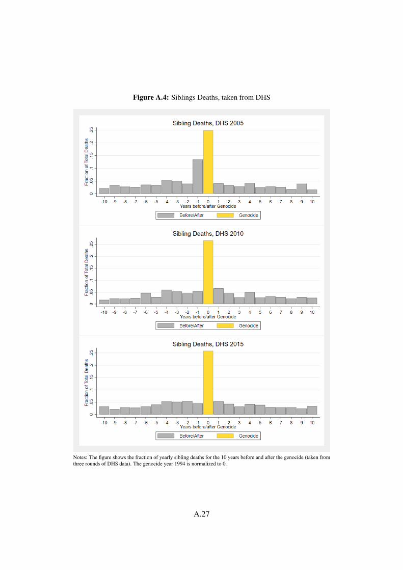
Figure A.4: Siblings Deaths, taken from DHS
Notes: The figure shows the fraction of yearly sibling deaths for the 10 years before and after the genocide (taken fromthree rounds of DHS data). The genocide year 1994 is normalized to 0.
A.27

Figure A.5: Siblings Deaths Regressions, taken from DHS
Notes: The figures show the distribution of coefficients on the instrument when using the number of sibling deaths fordifferent years (taken from three rounds of DHS data) in my preferred specification (regressions 3 and 6 in Panel A inTable 3 in the paper). The genocide year is normalized to 0. None of the coefficients are larger in absolute value thanthe one from 1994.
A.28

Table A.12: Refugees and Internally Displaced People and RPF
Panel A. Internally Number of DaysDependent Variable: Refugee Displaced Under RPF Control
(1) (2) (3) (4)
Distance × Rainfall along Buffer, 1994 −0.001 0.010 −0.114 −0.077(0.013) (0.011) (0.073) (0.051)
Standard Controls yes yes yes yesGrowing Season Controls yes yes yes yesAdditional Controls yes yes yes yesHarvest Season Controls no no no yesProvince Effects yes yes yes yes
R2 0.27 0.05 0.90 0.90N 13028 12233 1432 1432
Panel B.Sample: Females Males Adult Males
Dependent Variable: Internally Internally InternallyRefugee Displaced Refugee Displaced Refugee Displaced
(1) (2) (3) (4) (5) (6)
Distance × Rainfall along Buffer, 1994 0.006 0.013 −0.009 0.007 −0.014 0.004(0.013) (0.011) (0.014) (0.011) (0.014) (0.008)
Standard Controls yes yes yes yes yes yesGrowing Season Controls yes yes yes yes yes yesAdditional Controls yes yes yes yes yes yesProvince Effects yes yes yes yes yes yes
R2 0.27 0.06 0.27 0.05 0.28 0.06N 7234 6810 5794 5423 3849 3600
Notes: In regression 1 the dependent variable is a dummy taking on the value of 1 if an individual was a refugee. Inregression 2 the dependent variable is a dummy taking on the value of 1 if an individual was internally displaced during thegenocide. The data is taken from the EICV1 Survey and includes all individuals for which migration data is available (above16 years old). In Panel B. I split the full sample into different subsets (given in the column header). Standard Controlsinclude village population, distance to the main road, rainfall in the village during the 100 days of the genocide in 1994,long-term average rainfall in the village during the 100 calender days of the genocide period (average for 1984-1993), rainfallalong the buffer during the 100 days of the genocide in 1994, long-term average rainfall along the buffer during the 100calender days of the genocide period (1984-1993), and the latter interacted with distance to the main road. Growing SeasonControls are rainfall during the growing season in 1994 in the village, ten-year long-term average rainfall during the growingseasons in the village and both of these interacted with the difference between the maximum distance to the main road inthe sample and the actual distance to the main road. Additional Controls are distance to Kigali, main city, borders, Nyanza(old Tutsi Kingdom capital) as well as population density in 1991 and the number of days with RPF presence (except forregressions 3 and 4 in Panel A.). Harvest Season Controls are rainfall along the way between village and main road duringthe harvest season and its interaction with distance to the main road. All control variables, except “Number of Days withRPF presence,” are in logs. Interactions are first logged and then interacted. There are 11 provinces in the sample. Standarderrors correcting for spatial correlation within a radius of 150km are in parentheses, Conley (1999).
A.29

Figure A.6: Construction of the Instrument in ArcGIS
Instrument: Interaction of the length of the red line and amount of rain falling on the area of the blue rectangle duringthe period of the genocide.
A.30
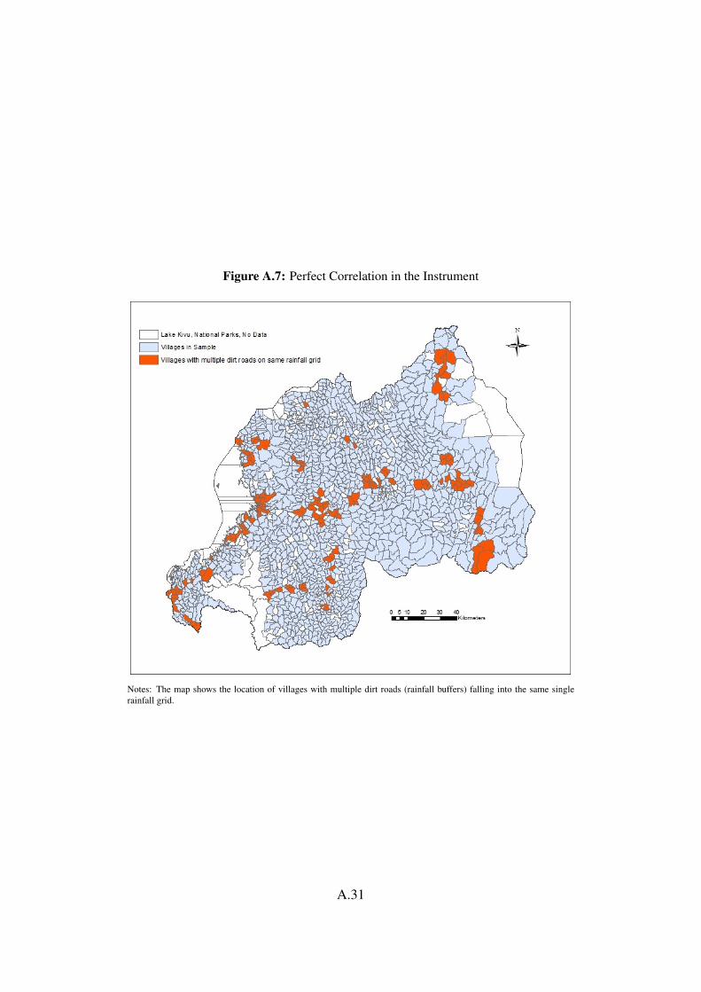
Figure A.7: Perfect Correlation in the Instrument
Notes: The map shows the location of villages with multiple dirt roads (rainfall buffers) falling into the same singlerainfall grid.
A.31

Figure A.8: Rainfall
Notes: This map shows rainfall along the way between main road and village during the period of the genocide in 1994for each village, subtracting rainfall between main road and village during the 100 calendar days of the genocide of anaverage year (years 1984-1993). White areas are either national parks, Lake Kivu, or villages not in the sample.
A.32

A.3 Extensions to Section III. – Understanding theFirst Stage
A.3.1 Understanding the First Stage
In this section I provide some additional results on the mechanisms of the instru-ment. Recall that I assume that the costs of traveling along the main roads arenegligible relative to the costs one has to occur when leaving those main roads,since local roads are usually non-paved dirt roads and heavy rains quickly makethem very difficult to penetrate with motorized vehicles. Rain turns dirt roadsinto slippery mud, usually requiring expensive four wheel drives and forcingdrivers to slow down; experts recommend about half the usual speed on wet dirtroads (ASIRT, 2005). Since the genocide planners were under time pressuretime was costly. Furthermore, water can collect in potholes and create deeppuddles or broken trees might block the road, requiring the driver to stop andclear the road or measure water depth, thus increasing travel time and costs evenfurther.15
Unfortunately, my satellite data does not allow me to identify whether anindividual dirt road was destroyed by the rain. However, I can provide somesuggestive evidence for the channels mentioned above. In particular, rainfall ondirt roads should make traveling harder in hilly areas. In Table A.13, I interactthe instrument with the slope along the way between the village and main road.16
The interaction effect is strongly negative as expected and almost significant(regression 1). In regression 2, I interact the instrument with a dummy takingon the value of one if the slope lies above the median. Again, the interactioneffect is negative and this time highly significant. Thus, it seems that rainfallincreases transport costs especially in hilly areas. As a robustness check, I showthat the main IV results are robust to using both my original instrument and itsinteraction with slope as instruments (regression 6).
Another important question is how persistent the effects of rainfall are. It
15Fallen trees are less of a problem for main roads since there is usually some space betweenroad boundary and the surrounding vegetation.
16I show results when using maximum slope along the way between village and main road.Results are robust to using average slope, albeit weaker. This makes sense given that the steepestpart should matter most. The data is downloaded from the USGS database (NASA and NGA,2000).
A.33
might be that rainfall before the genocide mattered too if roads got permanentlydamaged. Note that the instrument only uses rainfall for the exact period ofthe genocide. To show that this is a reasonable assumption I add distance tothe main road interacted with rainfall one week before the genocide to the firststage regression (regression 3). While the point estimate on my instrument (us-ing rainfall during the genocide) is identical to my baseline results the effect forrainfall one week before the genocide is small and insignificant. Besides, whenadding the interaction with rainfall two weeks before the genocide in regres-sion 4, the point estimate is even smaller and strongly insignificant (note thatthe effect for one week before turns significant, however this result is not ro-bust to clustering standard errors). Intuitively, although rainfall can create deeppotholes, once the dirt dries it usually becomes passable relatively quickly.
As a final sanity check, in regression 5, I interact the instrument with thestandard deviation of daily rainfall between the village and the main road. Thepoint estimate is positive and significant. Thus, the first-stage effects are weakerin areas with high temporal variation in rainfall. This is intuitive since hightemporal variation implies that there exist relatively dry time periods duringwhich a village could have easily been reached.
A.3.2 Extension: The Organizer’s Time Horizon
Intuitively, if the genocide planners had had unlimited time to complete thegenocide, I should not expect to find any effects in the first stage: Places thatwere hard to reach at the beginning of the genocide were likely easy to reachduring the end when the dry season started. However, because the genocideplanners did not know if and when the international community would inter-vene, any day could have been the last. Thus the planners rushed to executethe genocide as quickly as possible (taking into account transport costs). Thisimplies two things: we should observe the bulk of the killings in the first coupleof weeks and transport costs likely mattered less towards the end. Figure A.9plots the estimated total number of killings over time.17 Importantly, the bulk ofthe killings were perpetrated within the first couple of weeks. Besides, transport
17These estimates are also taken from Genodynamics.com and generated using a Bayesianlatent variable model on information from five different sources: the Ministry of Education inRwanda, the Ministry of Local Affairs in Rwanda, Ibuka (the Rwandan survivor organization),African Rights, and the Human Rights Watch.
A.34
costs seemed to have mattered the most at the beginning of the genocide and notat all towards the end. In Figure A.10, I split the genocide period into differ-ent intervals (3-week and 5-week intervals) and re-run my first-stage regression.While the point estimates for the first intervals are large and statistically sig-nificant at least at the 90 percent level, they are close to zero and insignificanttowards the end.
On a side note, I find exactly the same pattern in the reduced form usingcivilian perpetrators (Figure A.11). This provides some additional evidence thatit is really the militiamen driving the effects in the reduced form.
A.3.3 Extension: Main Road Costs
My first-stage analysis makes two assumptions. First, that transport costs onthe main roads are negligible relative to the costs for driving on dirt roads andsecond that armed groups took the shortest route from the main road to eachvillage. I now relax these two assumptions. In particular, I assume that armedgroups originated from the nearest main city (which is corroborated by anecdo-tal evidence) and that they did not necessarily take the shortest route from themain road to the village but rather the one with the lowest costs (accounting forboth distance and rainfall).18
In Table A.14, I show the results. Since I do not know the relative costs of1 mm of rainfall on a dirt road versus a tarred road, I present results for variouscosts. In regression 1, I calculate total travel costs assuming that the costs oftraveling on the main road are 50 percent lower than traveling on a dirt road.Recalculating the instrument under these assumptions gives a somewhat weakerfirst stage. I then re-calculate the instrument assuming that relative costs are20, 10, and 5 percent. In all cases the results are very similar to my baselinefirst-stage result from Table 3 in the paper. Besides, I also re-run the secondstage with the new instruments (20, 10 and 5 percent) and virtually obtain thesame point estimates (regressions 5 to 7). Taken together, these results suggestthat using the direct route between village and main road without taking intoaccount main road travel seems to be a reasonable approximation. Note thatwhen main road travel costs are about 20 percent of dirt road costs the first stage
18I allow militiamen to leave the main road 10 kilometers up and down the baseline point ofdeparture (i.e. when using the shortest path). I use the ArcGIS network tool to calculate theshortest path between the closest main city and the point where the dirt road begins.
A.35
gets equally strong as my baseline first stage. This is somewhat consistent withanecdotal evidence from Ethiopia (like Rwanda a very mountainous country)which suggests that average speed on a dirt road is about 25 to 30 percent of theaverage speed on a tarred road (Briggs, 2012).19
19Note that this comparison is likely an upper bound since it also factors in the dry season. Inmy Rwanda sample, I always observe positive rainfall.
A.36

References
[1] National Aeronautics and Space Administration (NASA) and NationalGeospatial-Intelligence Agency (NGI). 2000. Shuttle Radar TopographyMission digital elevation model (SRTM30), provided by United States Ge-ological Survey, https://dds.cr.usgs.gov/srtm/version2 1/SRTM30/e020n40/(accessed January 2014).
[2] Association For Safe International Road Travel(ASIRT). 2005. Road Security Report: South Africa,http://www.wpi.edu/Images/CMS/GPP/South Africa.pdf.
[3] Briggs, Philip. 2012. Ethiopia – the Bradt Travel Guide, Guilford, Con-necticut: The Global Pequot Press Inc.
A.37

Figure A.9: Killings over Time
Notes: The figure plots the estimated number of total deaths over time. These estimates are taken from Genodynam-ics.com and generated using a Bayesian latent variable model on information from five different sources: the Ministryof Education in Rwanda, the Ministry of Local Affairs in Rwanda, Ibuka (the Rwandan survivor organization), AfricanRights, and the Human Rights Watch.
A.38
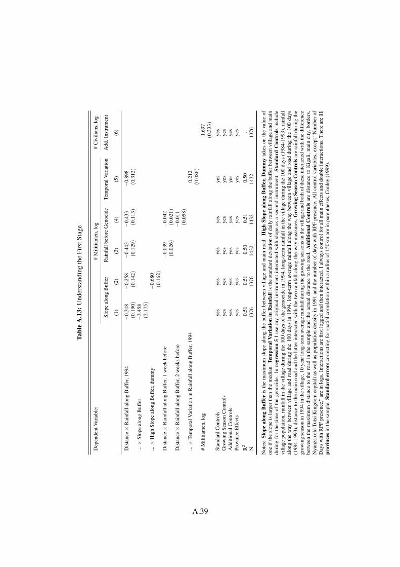
Tabl
eA
.13:
Und
erst
andi
ngth
eFi
rstS
tage
Dep
ende
ntV
aria
ble:
#M
ilitia
men
,log
#C
ivili
ans,
log
Slop
eal
ong
Buf
fer
Rai
nfal
lbef
ore
Gen
ocid
eTe
mpo
ralV
aria
tion
Add
.Ins
trum
ent
(1)
(2)
(3)
(4)
(5)
(6)
Dis
tanc
e×
Rai
nfal
lalo
ngB
uffe
r,19
94−
0.31
8−
0.25
8−
0.44
3−
0.43
3−
0.89
8(0
.190)
(0.1
42)
(0.1
29)
(0.1
13)
(0.3
12)
...×
Slop
eal
ong
Buf
fer
−3.
458
(2.1
75)
...×
Hig
hSl
ope
alon
gB
uffe
r,du
mm
y−
0.68
0(0
.162)
Dis
tanc
e×
Rai
nfal
lalo
ngB
uffe
r,1
wee
kbe
fore
−0.
039
−0.
042
(0.0
26)
(0.0
21)
Dis
tanc
e×
Rai
nfal
lalo
ngB
uffe
r,2
wee
ksbe
fore
−0.
011
(0.0
58)
...×
Tem
pora
lVar
iatio
nin
Rai
nfal
lalo
ngB
uffe
r,19
940.
212
(0.0
86)
#M
ilitia
men
,log
1.69
7(0
.333)
Stan
dard
Con
trol
sye
sye
sye
sye
sye
sye
sG
row
ing
Seas
onC
ontr
ols
yes
yes
yes
yes
yes
yes
Add
ition
alC
ontr
ols
yes
yes
yes
yes
yes
yes
Prov
ince
Eff
ects
yes
yes
yes
yes
yes
yes
R2
0.51
0.51
0.50
0.51
0.50
.N
1376
1376
1432
1432
1432
1376
Not
es:
Slop
eal
ong
Buf
fer
isth
em
axim
umsl
ope
alon
gth
ebu
ffer
betw
een
villa
gean
dm
ain
road
.H
igh
Slop
eal
ong
Buf
fer,
Dum
my
take
son
the
valu
eof
one
ifth
esl
ope
isla
rger
than
the
med
ian.
Tem
pora
lVar
iatio
nin
Rai
nfal
lis
the
stan
dard
devi
atio
nof
daily
rain
fall
alon
gth
ebu
ffer
betw
een
villa
gean
dm
ain
duri
ngfo
rth
etim
eof
the
geno
cide
.In
regr
essi
on5
Ius
em
yor
igin
alin
stru
men
tin
tera
cted
with
slop
eas
ase
cond
inst
rum
ent.
Stan
dard
Con
trol
sin
clud
evi
llage
popu
latio
n,ra
infa
llin
the
villa
gedu
ring
the
100
days
ofth
ege
noci
dein
1994
,lon
g-te
rmra
infa
llin
the
villa
gedu
ring
the
100
days
(198
4-19
93),
rain
fall
alon
gth
ew
aybe
twee
nvi
llage
and
road
duri
ngth
e10
0da
ysin
1994
,lon
g-te
rmav
erag
era
infa
llal
ong
the
way
betw
een
villa
gean
dro
addu
ring
the
100
days
(198
4-19
93),
dist
ance
toth
em
ain
road
and
the
latte
rint
erac
ted
with
the
two
rain
fall-
alon
g-th
e-w
aym
easu
res.
Gro
win
gSe
ason
Con
trol
sare
rain
fall
duri
ngth
egr
owin
gse
ason
in19
94in
the
villa
ge,1
0ye
arlo
ng-t
erm
aver
age
rain
fall
duri
ngth
egr
owin
gse
ason
sin
the
villa
gean
dbo
thof
thes
ein
tera
cted
with
the
diff
eren
cebe
twee
nth
em
axim
umdi
stan
ceto
the
road
inth
esa
mpl
ean
dth
eac
tual
dist
ance
toth
ero
ad.
Add
ition
alC
ontr
ols
are
dist
ance
toK
igal
i,m
ain
city
,bor
ders
,N
yanz
a(o
ldTu
tsiK
ingd
omca
pita
l)as
wel
las
popu
latio
nde
nsity
in19
91an
dth
enu
mbe
rofd
ays
with
RPF
pres
ence
.All
cont
rolv
aria
bles
,exc
ept“
Num
bero
fD
ays
with
RPF
pres
ence
,”ar
ein
logs
.Int
erac
tions
are
first
logg
edan
dth
enin
tera
cted
.Ial
way
sco
ntro
lfor
allm
ain
effe
cts
and
doub
lein
tera
ctio
ns.T
here
are
11pr
ovin
cesi
nth
esa
mpl
e.St
anda
rder
rors
corr
ectin
gfo
rspa
tialc
orre
latio
nw
ithin
ara
dius
of15
0km
are
inpa
rent
hese
s,C
onle
y(1
999)
.
A.39

Figure A.10: First-Stage Effects over Time
Notes: I replace my instrument in regression 3 in Panel A in Table 3 by interactions of distance to the main roadwith rainfall along the way for three/five time intervals of equal length. The point estimates together with 95 percentconfidence intervals are plotted on the y-axis. To illustrate, the first point estimate on the left figure is on distance to themain road interacted with rainfall along the way during the first five weeks of the genocide.
Figure A.11: Reduced-Form Effects over Time
Notes: I replace my instrument in regression 6 in Panel A in Table 3 by interactions of distance to the main roadwith rainfall along the way for three/five time intervals of equal length. The point estimates together with 95 percentconfidence intervals are plotted on the y-axis. To illustrate, the first point estimate on the left figure is on distance to themain road interacted with rainfall along the way during the first five weeks of the genocide.
A.40

Tabl
eA
.14:
Alte
rnat
ive
Rou
tes
(inc
l.M
ain
Roa
ds)
Dep
ende
ntV
aria
ble:
#M
ilitia
men
,log
#C
ivili
anPe
rpet
rato
rs,l
og
(1)
(2)
(3)
(4)
(5)
(6)
(7)
Qui
ckes
tPat
h,M
ain
Roa
d50
%−
0.38
6(0
.095)
Qui
ckes
tPat
h,M
ain
Roa
d20
%−
0.46
9(0
.112)
Qui
ckes
tPat
h,M
ain
Roa
d10
%−
0.47
5(0
.116)
Qui
ckes
tPat
h,M
ain
Roa
d5%
−0.
481
(0.1
18)
#M
ilitia
men
,log
1.40
81.
377
1.35
8(0
.303)
(0.3
07)
(0.3
03)
Stan
dard
Con
trol
sye
sye
sye
sye
sye
sye
sye
sG
row
ing
Seas
onC
ontr
ols
yes
yes
yes
yes
yes
yes
yes
Add
ition
alC
ontr
ols
yes
yes
yes
yes
yes
yes
yes
Mai
nR
oad
Con
trol
sye
sye
sye
sye
sye
sye
sye
sPr
ovin
ceE
ffec
tsye
sye
sye
sye
sye
sye
sye
s
R2
0.50
0.50
0.50
0.50
..
.N
1432
1432
1432
1432
1432
1432
1432
Not
es:
The
inst
rum
ent
isth
eto
tal
tran
spor
tco
sts
alon
gth
edi
rtro
adan
dal
ong
the
mai
nro
ad.
For
exam
ple,
inQ
uick
est
Path
,Mai
nR
oad
50%
Ias
sum
eth
atth
etr
avel
cost
s(i
nduc
edby
rain
fall)
onth
em
ain
road
are
50pe
rcen
tof
thos
eon
the
dirt
road
.In
regr
essi
ons
5to
7,I
inst
rum
entf
orth
enu
mbe
rof
mili
tiam
enw
ithth
ein
stru
men
tfro
mre
gres
sion
s2
to4,
resp
ectiv
ely.
Stan
dard
Con
trol
sin
clud
evi
llage
popu
latio
n,di
stan
ceto
the
mai
nro
ad,r
ainf
alli
nth
evi
llage
duri
ngth
e10
0da
ysof
the
geno
cide
in19
94,l
ong-
term
aver
age
rain
fall
inth
evi
llage
duri
ngth
e10
0ca
lend
erda
ysof
the
geno
cide
peri
od(1
984-
1993
),ra
infa
llal
ong
the
“qui
ckes
t”w
ay(n
otne
cess
arily
shor
test
)be
twee
nvi
llage
and
mai
nro
addu
ring
the
100
days
ofth
ege
noci
dein
1994
,lon
g-te
rmav
erag
era
infa
llal
ong
the
“qui
ckes
t”w
aybe
twee
nvi
llage
and
mai
nro
addu
ring
the
100
cale
nder
days
ofth
ege
noci
depe
riod
(198
4-19
93)a
ndth
ela
tteri
nter
acte
dw
ithdi
stan
ceto
the
mai
nro
ad(a
gain
notn
eces
sari
lysh
orte
st).
Gro
win
gSe
ason
Con
trol
sand
Add
ition
alC
ontr
ols
are
defin
edin
Tabl
e3
inth
epa
per.
Mai
nR
oad
Con
trol
sar
edi
stan
ceto
the
clos
estm
ain
city
(mea
sure
dal
ong
the
mai
nro
adne
twor
kfr
omth
em
ain
city
toth
epo
intw
here
the
dirt
road
begi
ns)
and
rain
fall
alon
gth
ew
ay.
All
cont
rolv
aria
bles
,exc
ept“
Num
ber
ofD
ays
with
RPF
pres
ence
,”ar
ein
logs
.In
tera
ctio
nsar
efir
stlo
gged
and
then
inte
ract
ed.
The
rear
e11
prov
ince
sin
the
sam
ple.
Stan
dard
erro
rsco
rrec
ting
for
spat
ialc
orre
latio
nw
ithin
ara
dius
of15
0km
are
inpa
rent
hese
s,C
onle
y(1
999)
.
A.41
A.4 Extensions to Section III. – Placebo, ExclusionRestriction, and Robustness Checks
A.4.1 Placebo Tests
To rule out systematic measurement error in the rainfall data or that somethingother than the militia might be driving the results, I rerun both first-stage andreduced-form regressions using rainfall during the 100 calendar days of thegenocide from the years 1983 until 2014 in the instrument. Reassuringly, thecoefficient on the instrument with rainfall from 1994, the year of the genocide,is an outlier to the left in the distribution of 32 point estimates (Figures A.12 andA.13). Besides, the figures show that the strong negative effect for the genocideperiod from 1994 is not simply the result of a negative long-term trend: the pointestimates for the time periods before 1994 are all oscillating around zero.
Moreover, I also rerun first stage and reduced form using rainfall for various100-day windows before and after the genocide in the instrument. Again, thecoefficient on the instrument with rainfall during the genocide is an outlier inboth cases (Figures A.14 and A.15).20
Finally, rerunning the two placebo checks from above with child mortality(from the EICV survey) or the number of Tutsi deaths (from Genodynamics) asthe dependent variable gives similar results: the coefficient on the instrumentwith 1994 rainfall during the genocide period is an extreme outlier in all cases(Figures A.16, A.17 and A.18).
A.4.2 Exclusion Restriction Tests
At this point, I still need to argue that civilians were not directly affected bythe instrument, i.e. by traveling themselves, or that the instrument somehowaffected access to markets, prices and income.
Anecdotal Evidence Starting with anecdotal evidence, several reports and ac-counts of the genocide indeed support the claim that civilian violence was a very
20This also rules out that the results may be driven by some non-linear effects of distance tothe main road (this should then be true for other time periods as well).
A.42
local affair (Hatzfeld, 2005).21
Besides that, few people in Rwanda, let alone ordinary civilians, owned acar or a truck (less than 1 percent according to the 1992 DHS Survey) and thepossibilities of moving between villages in motor vehicles, certainly the mostaffected by rain-slickend roads, were therefore limited for civilians. In addition,moving around along or close to the main roads was risky for ordinary citizens,as roadblocks were set up all over the country and being Hutu did not alwaysensure safety. Prunier (1995, p. 249) writes that “To be identified on one’s
[identity] card [often at a roadblock] as a Tutsi or to pretend to have lost one’s
paper meant certain death. Yet to have a Hutu ethnic card was not automati-
cally a ticket to safety. (...) And people were often accused of having a false
card, (...).” Amnesty International (1994, p. 6) reports that “Each individual
passing through these roadblocks had to produce an identity card which indi-
cates the ethnic origin of its bearer. Being identified as or mistaken for a Tutsi
meant immediate and summary execution.” Des Forges (1999, p. 210) contin-ues, “During the genocide some persons who were legally Hutu were killed as
Tutsi because they looked Tutsi. According to one witness, Hutu relatives of Col.
Tharcisse Renzaho, the prefect of the city of Kigali, were killed at a barrier after
having been mistaken for Tutsi.”
Furthermore, there were no reasons for Hutu to travel because social lifecompletely stopped (Hatzfeld, 2005). As one civilian killer puts it, “During the
killings, we had not one wedding, not one baptism, not one soccer match, not
one religious service like Easter.” (Hatzfeld, 2005, pp. 94-95). Another onecontinues (p. 133), “During the killings there was no more school, no more
leisure activities, no more ballgames and the like.”
On a more general account, Horowitz (2001, p. 526) notes “that [civil-
ian] crowds generally stay close to home, attack in locales where they have
the tactical advantage, and retreat or relocate the attack when they encounter
unexpected resistance.”
Curfew Test Besides the anecdotal evidence, I also present a number of in-direct tests. At the beginning of the genocide, a strict nation-wide curfew wasimplemented, which drastically limited the travel opportunities for civilians –
21Hatzfeld (2005) calls it a Neighborhood Genocide because only neighbors and co-workerswere able to identify Tutsi, as they are similar to the Hutu (Hatzfeld, 2005).
A.43
in fact both Hutu and Tutsi were required to stay at home. Des Forges (1999,p. 162) writes that “At the start, authorities instructed Rwandans to stay at
home. The curfew allowed authorities and local political leaders to put in place
the barriers and patrols necessary to control the population, multiplying them
in communities where they were already functioning and reestablishing them in
places where they were no longer in operation. Tutsi as well as Hutu cooper-
ated with these measures at the start, hoping they would ensure their security.
The hope was disappointed.” Reassuringly, the instrumental-variables estimatesare similar to the baseline results when I restrict the variation in rainfall in theinstrument to the first five days, the first week, or the first two weeks of thegenocide, while controlling for rainfall along the way between village and mainroad for the remaining days and its interaction with distance to the main road(regressions 1 to 3 in Table A.15 below).22 I believe that this is a very powerfultest since the curfew essentially ruled out any kind of civilian movement.
Commune Test Next, because of tight population controls, already before1994, it was practically impossible for civilians to get permission to leave theircommune. The authorities carefully monitored and controlled the population.Des Forges (p. 186, 1999) writes “Rwandans were supposed to be registered
in the communes of residence if these differed from their communes of birth.
Nyumbakumi, cell heads, and councilors all were involved in making sure that
no strangers lived unnoticed in a commune.” Des Forges (pp. 186) continuesthat “Authorities also revived an earlier requirement that persons wishing to
travel outside their communes receive written authorization to leave (feuilles de
route).” Thus leaving one’s commune involved significant costs. And indeed theresults are similar, if anything larger, when I restrict the sample to those com-munes with no main road passing through (regression 4 in Table A.15). Thisfurther supports the identification strategy since moving around the communeshould have been unrelated to transport costs in these off-the-main-road areas.
The two tests above provide general evidence that the exclusions restriction
22To be cautious, I also control for the long-term average rainfall between village and mainroad for those first couple of days and its interaction with distance to the main road as well asrainfall in the village during the first couple of days and its long-term average. Furthermore, I usedifferent cutoff dates because I do not know when exactly the curfew ended. For the first-five-days and first-week regressions, I lose a few observations, because there was no rainfall duringthat short time period. However, rerunning the baseline regression with those two reducedsamples gives the same results.
A.44

is likely to hold. In the following I will work through several possible threats– providing evidence why they should not matter (occasionally drawing on thetwo tests above).
Civilians Escaping There are two possibilities. High transport costs mighthinder civilians from escaping (in case they took the main road). This scenariohowever would only work against my findings and bias the estimate downwards.On a side note, it seems unlikely since road blocks were set up all over thecountry and civilians likely avoided those under all circumstances. The otherpossibility is that civilians could easily flee from places that the militia couldnot reach (because of high transport costs). A number of results suggest thatthis is unlikely. First, as noted above at the beginning of the genocide the strictcurfew forced people to stay at home and even Tutsi cooperated with these or-ders. Second, escaping the violence – because of high transport costs – shouldhave been less of an issue in places close to the border since here civilians likelymanaged to escape much easier anyway. Importantly, in regression 5 in TableA.15 I show that the effects of the militia do not depend on the distance to theborder. If anything the effects are slightly larger close to the border. Finally,recall from the discussion above that I do not find any evidence that becoming arefugee or being internally displaced during the genocide is correlated with theinstrument.
Civilians Getting Stuck In The Fields Another concern is that civilians whowork their fields further from home close to the main dirt road get stuck andcannot return home if transport costs are high. This case is also unlikely forseveral reasons. First, as noted above Rwandans were only occasionally givenpermission to leave the commune, it therefore seems highly unlikely that theyhad fields outside of their home commune – which they would have neededto access every day. Thus the second test from above speaks against this con-cern. Second, recall again that the curfew prevented civilians from leaving theirhomes, thus they unlikely worked on their fields. Finally, recall from above thatvery few civilians owned a car or truck and most of the farmers movements thushappened on foot. However, while strong rainfalls do affect vehicle transporta-tion, they are unlikely to keep individuals from returning home.
A.45

Public Transportation The instrument might also affect public transportationfor civilians. Again, it seems unlikely that this mattered. First, the curfew re-quested everyone to stay at home, thus civilians unlikely took a local bus or cab.Besides, public transportation is likely more common in urban areas. Below, Ishow that the results are robust to dropping all the main cities and the capitalKigali (Table A.23).
Localized Violence Unfortunately, the raw Gacaca data only records the lo-cation where people committed their crime(s) and not where they lived. A po-tential concern is thus that civilians traveled together with the militia and jointlycommitted the crimes (the curfew does not fully address this issue because civil-ians may have been granted permission to travel by the authorities). I addressthis in two ways: first, I did not find any anecdotal evidence that civilians fol-lowed the militia on their killing spree (naturally, this does not rule out the coun-terfactual but it is somewhat comforting). Second and more importantly, thesame government agency that provided the Gacaca data (“National Service ofGacaca Jurisdiction”) also provided a spreadsheet of a random subset of 20,000category 2 perpetrators including names, sex, home village and the locationsof where the crimes were committed (around 2.5 percent are female). Given atotal of about 430,000 category 2 cases, this number is large enough to allow forrepresentativeness.
Importantly, only about 4 percent of the individuals in this sample commit-ted crimes outside of their home village. However, in all these cases the crimesare committed within the home commune. This suggests that it is unlikely thatlarge numbers of civilians joined the militia outside of their home areas butrather stayed within their home village (or in a few cases communes). Note thatcivilians moving within a commune is unlikely to bias the results. First, the datasuggests that this only happened in very few cases (i.e. 4 percent) and secondrecall from regression 4 in Table A.15 that the results are robust to excludingcommunes that have a main road passing through. Thus it seems unlikely thatcivilians’ decisions to commit crimes in their neighboring villages are affectedby the instrument.
Market Access and Income/Price Effects Transport costs may have also af-fected civilians’ access to markets (often located close to the main road) and
A.46

thus potentially prices and income which in turn could affect participation inviolence. Importantly, the timing of the genocide somewhat alleviates this con-cern. It partly overlaps with the growing season which ensures enough variationin rainfall to affect transport costs (there is essentially no rainfall during the dryseason) but still allows me to control for rainfall during the growing season.Besides, the harvest season and thus the time when villagers take their crops tothe market to sell (and hence transport costs should matter) only accounts fora small period during the end of the genocide. I first show that my results arerobust to adding harvest season controls to the regressions (rainfall along thebuffer between village and main road during the harvest season and its interac-tion with distance to the road). First stage, reduced form and the main regressionare shown in Table A.16. Importantly, transport costs during the harvest seasondo not affect the first stage or reduced form (regressions 1 and 2) and neither dothey affect the main result (regression 3). Besides, the point estimate on harvestcosts is small and insignificant.
In the following, I show that rainfall during the genocide period interactedwith distance to the main road does not have an effect on wealth and income(once harvest costs are controlled for) for three different outcomes: a) TableA.17 uses nightlight density aggregated at the commune level;23 b) Table A.18uses information on household assets from the 1991 census to construct a wealthindex (also only available at the commune level);24 c) Table A.19 uses data onhousehold consumption, assets and agricultural income/output from the EICVhousehold survey from 2000/01. Finally, I can use the EICV household sur-vey to calculate local market prices for the major crops – again, transport costs(during the period of the genocide) have no effects on any of these (Table A.20).
In each case transport costs are constructed using rainfall from the year ofthe outcome data, i.e. 1991 rainfall for the 1991 census.25 Importantly, the in-teraction between rainfall during the genocide period and distance to the main
23Several satellites of the US Air Force circle around the earth 14 times a day observing everylocation on the planet at some instant between 8 and 10 pm local time. Each satellite datasetconsists of a grid that reports the average yearly light density with a six-bit digital number (aninteger between 0 and 62). The grid comes at a very high resolution, equal to approximately0.86 square kilometers at the equator. The data is provided by the NOAA (1992/1993).
24The index incorporates information on housing such as roofing and floor material, as wellas radio ownership and access to electricity and water.
25To be cautious, in those cases where the outcome variable is measured after 1994, I alsocontrol for distance to the main road interacted with rainfall along the buffer during the 100genocide days in 1994 and all main effects. Unsurprisingly, the results do not depend on it.
A.47

road is never significantly related to any income or wealth measure. Interest-ingly though, transport costs during the harvest season are often significant andshow the right sign, i.e. higher transport costs during the harvest season (andselling season) tend to decrease income and wealth (this is comforting becauseit shows that I am not simply obtaining noisy estimates). There is no clear re-lationship for crop prices. However this is unsurprising since there is no clearprediction in this case – whether harvest costs increase or decrease prices de-pends on local supply and demand. Most importantly, transport costs during thegenocide period are unrelated to crop prices. Some of the regressions are run atthe commune level. However, my baseline results are robust to collapsing thedata at that level (regression 1 in Table A.18).
Coffee Finally, one of Rwanda’s most important cash crops is coffee. Coffeeproduction is a very transport-intensive undertaking since it requires the coffeebeans to be shipped to special coffee mills for processing before being baggedand possibly exported. Thus if my instrument had effects not only on the mili-tia’s transport costs but also on the coffee production process I might obtain verydifferent results in areas with high coffee production or places with a coffee mill.
Thus, to check whether my results differ in coffee production places I usetwo additional data sets. One is a nation-wide survey on the number of coffeetrees in each village. Unfortunately that survey is from 1999 (5 years after thegenocide) but it includes information on the age of the tree. I can distinguishbetween trees planted before 1990 and after (“old” and “new” trees). The seconddata set contains information on the location of coffee mills that were installedby the 1960s. This data is taken from Guariso and Verpoorten (2018b).26
As a first test, I show in Table A.21 that my main effects are not significantlydifferent in places with coffee trees (regressions 1 to 3). The interaction effectsof the number of militiamen with the number of coffee trees in each village aresmall and insignificant. This is true when looking at all trees and old or new treesseparately. Besides, the interaction effects with the instrument are further smalland insignificant in the first stage (regressions 4 to 6). Finally, the instrument isuncorrelated with the number of coffee trees in each village (regressions 7 to 9).
26Although this data is seemingly old, it still predicts for example investment in coffee treemaintenance from 2003 (Guariso and Verpoorten, 2018a). Thus it seems reasonable to assumethat many of these mills are either still running or were replaced.
A.48

As a second test, I use the location of coffee mills. Results are reported inTable A.22. First, I show that the main results are robust to dropping villageswith a coffee mill (regression 1), villages with a coffee mill within 10 kilometers(regression 2) and within 20 kilometers (regression 3). Besides, the results arenot significantly different in any of these three subsets of villages (regressions4 to 6). Interaction effects are insignificant throughout. Finally, the first-stageeffects are not significantly different in villages with a coffee mill or coffee millsclose-by (regressions 7 to 9).
Gauging the Bias Thus taken together all of the above findings, includingthe abundance of anecdotal evidence (or sometimes rather absence of anecdotalevidence) suggests that the exclusion restriction is likely to hold.
To nevertheless get a sense of how large the direct effect of transport costson civilian violence would have to be to render the IV estimate insignificant,I follow Conley et al.’s (2012) plausibly exogenous method. I assume that the(potential) direct effect of the instrument on civilian violence is uniformly dis-tributed on an interval [δ ,0]. By varying δ , I identify the threshold at which theinstrumental variable coefficient on (instrumented) militia violence becomes in-significant at the 90 percent level. The results are reported in Figure A.19. Aslong as the direct effect of my instrument on civilian violence is smaller (in ab-solute value) than -0.5, I still obtain a significant instrumental variable estimate.In terms of magnitudes this suggest that the direct effect has to be 76 percent ofthe overall reduced-form effect to render the estimates insignificant. This seemshighly implausible given all the evidence from above together with the fact thatthere is no anecdotal evidence for systematic shipping of civilian perpetrators.
A.4.3 Robustness Checks
General Checks Next, I perform a number of general robustness checks, re-ported in Table A.23. Besides worrying about transport costs during the harvestseason from 1994, which I already discussed in more detail above, one mightfurther worry that yearly long-term rainfall might bias the results. Moreover,ruggedness might be correlated with rainfall and directly affect civilian partici-
A.49
pation in violence.27 However, the main effects is unaffected by controlling fora) the yearly long-term average rainfall in the village and along the way betweenvillage and main road and the interaction of the latter with distance to the mainroad, b) the interaction of distance to the main road with both rainfall in thevillage during the growing season in 1994 and long-term average rainfall in thevillage during the growing seasons, and c) village terrain ruggedness.
To check whether armed groups might have taken a direct route to eachvillage, possibly affected by rainfall along the way, I also control for rainfallduring the genocide along the way between each village and the closest maincity and its interaction with distance to the main city. As noted, I do not knowexactly where armed groups were stationed, but the vast majority are likely tohave started out from the main cities. However, the two additional controls donot affect the main result (regression 3). I provide a more detailed discussion inSection A.3 above. Furthermore, the results are robust to dropping all the maincities and villages close to them (regression 4).
One might also be worried that the UN troops that were stationed in Kigali,although few, were affected by transport costs, thus biasing the estimates. Butagain, the results are robust to dropping villages in Kigali city (regression 5).
Replacing 11 province fixed effects by 142 commune effects also does notmatter (regression 6). Since the rainfall data only comes at a coarse resolution,at least relative to the large number of communes, this significantly reducesthe variation in the instrument. Nevertheless, the instrumental-variables pointestimate remains similar and equally significant.
Temperature Besides, recent studies found that temperature can also havea direct impact on violence (Burke et al., 2015; Ranson, 2014; Hsiang et al.,2013). Given the correlation across climatic factors and in order to avoid anyomitted variables bias, in Table A.24 I add controls for temperature in the villageand along the way from the village to the main road as well as the interactionof the latter with distance to the main road. I report IV estimates (regressions 1to 4), as well as reduced-form estimates (regressions 5 to 8) and the first stage(regressions 9 to 12). Reassuringly, all the results are robust. This is true for
27The Terrain Ruggedness Index data is provided by Nunn and Puga (2012b) used in Nunnand Puga (2012a). The average villages ruggedness in my sample is 3.45 with a standard devi-ation of 1.38.
A.50

using both average temperature as well as maximum temperature. The temper-ature data is provided by the Terrestrial Hydrology Research Group and is alsoavailable daily at 0.1 degree resolution (Chaney et al., 2014).28
Dependent Variable To show that my findings are not dependent on func-tional form I report the results for alternative transformations of the dependentvariables in Tables A.25 and A.26. Most importantly, I obtain very similar re-sults when using a simple linear regression. The point estimate in regression 1 inTable A.25 suggests that an additional militiaman resulted in 6.8 more civilianperpetrators, very similar to my baseline results from above (recall: 7.2). Theresults are further robust to using a Poisson IV model (regression 2). The pointestimate translates into a marginal effect of around 6 (evaluated at the mean ofall the other variables). Moreover, the results are robust to using the number ofperpetrators normalized by local village population (regressions 3 and 4).
Finally, I vary the various log transformations. Importantly, the results arerobust to using a hyperbolic sine transformation – a common approach whendealing with observations that can take on the value of 0 (regression 1 in TableA.26). The point estimate is virtually identical to my baseline results. In regres-sions 2 to 9, I report results for various log(X+k) transformations where k variesbetween 0.0001 and 1000 (and X is either the number of militiamen or civilianperpetrators). The point estimates are only slightly lower for smaller k’s. To geta sense of the magnitude, the one for k = 0.0001 still implies that an additionalmilitiamen resulted in around 6 more civilian perpetrators.
Outliers To test for outliers, I also dropped one province at a time and the re-sulting estimates range from 1.153 to 1.527 and are significantly different fromzero at the 99 percent confidence level in all cases (Figure A.20).
Sensitivity Analysis Next, in Table A.27 I perform a standard sensitivity anal-ysis on the IV estimate, varying the number of controls. Altonji et al. (2005)derive a measure that determines how strong the unobservables have to be rel-ative to the already included observables to drive the point estimate down tozero. The controls for the unrestricted model (relative to which the other ones
28The data is available here: https://hydrology.princeton.edu/data.metdata africa.php.
A.51

are evaluated) are shown in column 1. In columns 2 to 7 I keep adding con-trols for the restricted models. For instance the number in column 3 suggeststhat the unobservables have to be 11.71 times as strong as the observables toeliminate the effect (controlling for all standard controls, growing season con-trols, additional controls and province fixed effects). To put this number intoperspective note that the observables in this case include strong predictors ofcivilian violence such as population and population density, distance to Kigali,province fixed effects, rainfall in the village and all growing season controls(among others). Importantly, the ratio is strongly above 1 for all specifications.Thus it seems unlikely that some other (unobservable) variable might alter themain result.
Robustness Check – Rainfall in Village The 11 kilometer rainfall grids mightbe too coarse to sufficiently distinguish between rainfall along the distancebuffer and rainfall in the village. Thus, the instrument might pick up differentialvillage rainfall effects rather than transport costs. For instance, rainfall in thevillage likely affects rain-fed agriculture and this channel is potentially strongerfor remote villages that depend on subsistence farming. Thus little rainfall invillages far away from the main road might lower villagers’ opportunity costsof violence – violating the exclusion restriction. Alternatively, villages close tothe main road that receive a lot of rainfall might be significantly richer not onlybecause they can harvest more but also because they can sell their products onthe nearby markets.
First note that these concerns are somewhat eased by the exact timing of thegenocide: it only partially overlaps with the growing season (the rainfall thatmatters the most for plant production and thus the two income channels out-lined above). Thus, in my main specifications I always control for rainfall inthe village during the 1994 spring growing season and also allow the villagegrowing season effects to vary by distance to the main road. As shown abovethe results are also robust to controlling for rainfall during the harvest season(the time when transport costs matter most for agricultural income) and its in-teraction with distance to the road. These controls should pick up most of thetwo economic effects outlined above.
However, to further alleviate these concerns, I also control for rainfall inthe village during the 100 genocide days in 1994 interacted with distance to the
A.52

main road for various specifications. Results are reported in Panel A of TableA.28. To show that the instrumental variable regressions are really driven by thearmed groups’ transport costs, I also report the first stage in Panel B. In regres-sion 1, I simply control for my crucial standard and growing season controls.Importantly, the IV results hold up and the interaction with rainfall along thebuffer rather than in the village seems to be driving the first stage – while thecoefficient on the former is large and almost significant at the 90 percent level,the one on the latter is small and strongly insignificant. In regressions 2 to 4, Iadd various other controls. For instance, for the sake of interpretation, I also addrainfall at the nearest point on the main road29 and its interaction with distanceto the main road. Although this is a very demanding specification, the IV esti-mates hold up. The first-stage point estimates drop a little. To increase power Idrop the province fixed effects in regression 5 and onwards (note that this doesnot change the effect in my baseline regression).30 In this case, the point esti-mates on the instrument increase (in absolute terms) and gain significance at the90 percent level while both rainfall in the village and at the main road (inter-acted with distance to the road) are relatively smaller and insignificant. I showseveral different specifications to ensure that the larger effect for the instrumentis not due to some lucky choice of suitable controls.
Taken together, this supports that the results are driven by rainfall along theway to the village (neither the interaction of distance to the main road with vil-lage rainfall nor with rainfall at the main road matter). Importantly, there is stillreasonable variation between rainfall in the village, rainfall at the main road,and rainfall along the buffer even for small distances because main roads, dis-tance buffers, and village boundaries are not perfectly aligned with the rainfallgrid but rather crisscross the grid cells in various locations.31
29Measured two and a half kilometers up and down the road (from the nearest point) over a500-meter road buffer. Results are robust to varying the 2.5 km cutoff.
30Dropping province fixed effects in my baseline regressions (regressions 3 in Panel A and 6in Panel B in Table 3) gives point estimates of 1.280 in the second stage and -0.798 in the firststage.
31For instance, rainfall along the buffer and in the village only fall within the same rainfallgrid for about 9 percent of the villages.
A.53
References
[1] Altonji, J.G., Elder, T.E. and C.R. Taber. 2005. An Evaluation of Instru-mental Variable Strategies for Estimating the Effects of Catholic Schooling.Journal of Human resources, 40(4): 791-821.
[2] Burke, M., Hsiang S. and E. Miguel. 2015. Climate and conflict. Annual
Review of Economics, 7: 577-617.
[3] Chaney, N. W., Sheffield, J., Villarini, G., and E. F. Wood 2014. De-velopment of a high-resolution gridded daily meteorological dataset oversub-Saharan Africa: spatial analysis of trends in climate extremes. Journal
of Climate, 27(15): 5815-5835.
[4] Conley, T.G., Hansen, C.B. and P.E. Rossi. 2012. Plausibly exogenous.Review of Economics and Statistics, 94(1): 260-272.
[5] Des Forges, A. 1999. Leave None to Tell the Story: Genocide in Rwanda,New York: Human Rights Watch.
[6] NOAA National Geophysical Data Center. 1992/1993. Version 4 DMSP-OLS Nighttime Lights Time Series: Average Visible, Stable Lights, &Cloud Free Coverages. DMSP data collected by US Air Force WeatherAgency. https://ngdc.noaa.gov/eog/dmsp/downloadV4composites.html (ac-cessed 2009).
[7] Guariso A. and M. Verpoorten. 2018a. Aid, trade and the post-war recov-ery of the Rwandan coffee sector. Journal of Eastern African Studies, 12(3):552-574.
[8] Guariso A. and M. Verpoorten. 2018b. Data for: Aid, trade and the post-war recovery of the Rwandan coffee sector. Journal of Eastern African Stud-
ies, 12(3): 552-574. (Data requested and received directly from the authors).
[9] Hatzfeld, J. 2005. Machete season: The Killers in Rwanda speak, NewYork: Picador.
[10] Horowitz, D. 2001. The Calculus of Passion, in: The Deadly Ethnic Riot,University of California Press, Berkeley, pp. 522-565.
A.54

[11] Hsiang, S. M., Burke, M. and E. Miguel. 2013. Quantifying the Influenceof Climate on Human Conflict, Science, 341(6151): 1235367.
[12] Nunn, N. and D. Puga. 2012a. Ruggedness: The Blessing of Bad Geog-raphy in Africa, The Review of Economics and Statistics, 94(1): 20-36.
[13] Nunn, N. and D. Puga. 2012b. Data and replication files for ’Ruggedness:The blessing of bad geography in Africa.’ Grid-cell-level data on terrainruggedness, Terrain Ruggedness Index, https://diegopuga.org/data/rugged/(accessed 2014).
[14] Ranson, M. 2014. Crime, Weather, and Climate Change. Journal of Envi-
ronmental Economics and Management, 67(3): 274-302.
A.55
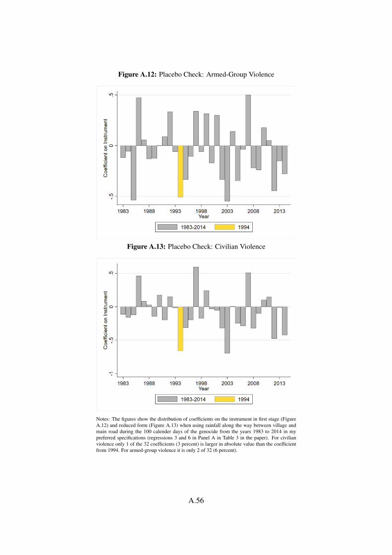
Figure A.12: Placebo Check: Armed-Group Violence
Figure A.13: Placebo Check: Civilian Violence
Notes: The figures show the distribution of coefficients on the instrument in first stage (FigureA.12) and reduced form (Figure A.13) when using rainfall along the way between village andmain road during the 100 calender days of the genocide from the years 1983 to 2014 in mypreferred specifications (regressions 3 and 6 in Panel A in Table 3 in the paper). For civilianviolence only 1 of the 32 coefficients (3 percent) is larger in absolute value than the coefficientfrom 1994. For armed-group violence it is only 2 of 32 (6 percent).
A.56
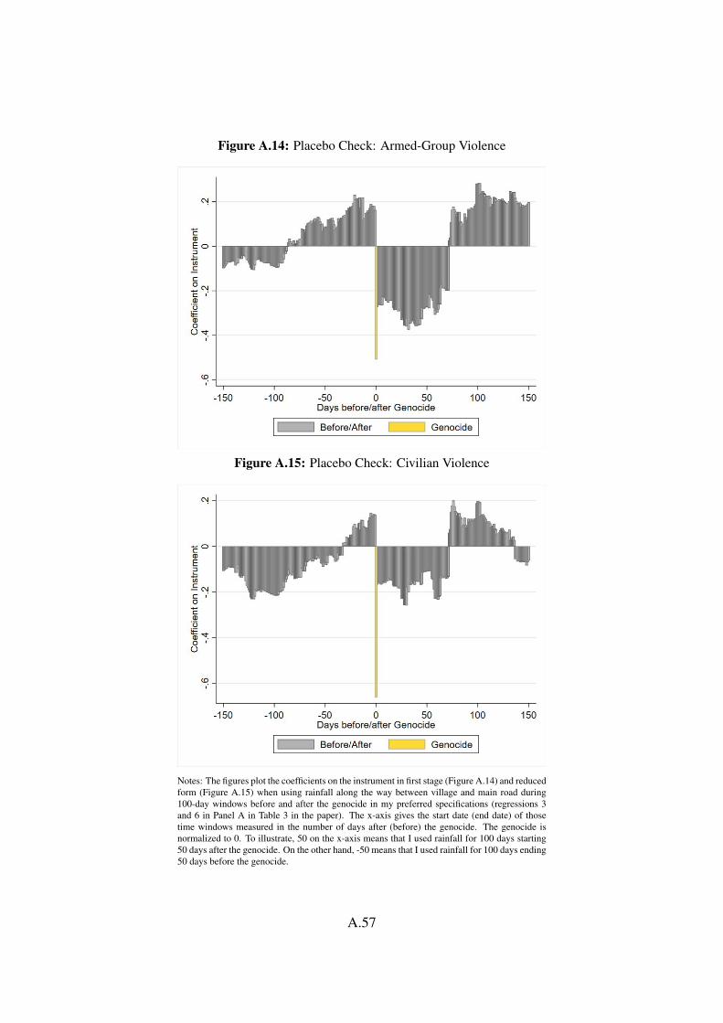
Figure A.14: Placebo Check: Armed-Group Violence
Figure A.15: Placebo Check: Civilian Violence
Notes: The figures plot the coefficients on the instrument in first stage (Figure A.14) and reducedform (Figure A.15) when using rainfall along the way between village and main road during100-day windows before and after the genocide in my preferred specifications (regressions 3and 6 in Panel A in Table 3 in the paper). The x-axis gives the start date (end date) of thosetime windows measured in the number of days after (before) the genocide. The genocide isnormalized to 0. To illustrate, 50 on the x-axis means that I used rainfall for 100 days starting50 days after the genocide. On the other hand, -50 means that I used rainfall for 100 days ending50 days before the genocide.
A.57

Figure A.16: Placebo Check: Child Mortality – Different Years
Figure A.17: Placebo Check: Child Mortality – Different Time Windows
Notes: Figure A.16 shows the distribution of coefficients on the instrument when using rainfallalong the way between village and main road during the 100 calender days of the genocide fromthe years 1983 to 2014 in regression 1 in Table A.9 in the paper.Figure A.17 plots the coefficients on the instrument when using rainfall along the way betweenvillage and main road during 100-day windows before and after the genocide in regression 1in Table A.9 in the paper. The x-axis gives the start date (end date) of those time windowsmeasured in the number of days after (before) the genocide. The genocide is normalized to 0.To illustrate, 50 on the x-axis means that I used rainfall for 100 days starting 50 days after thegenocide. On the other hand, -50 means that I used rainfall for 100 days ending 50 days beforethe genocide.
A.58

Figure A.18: Placebo Check: Death Estimates
Notes: The figures show the distribution of coefficients on the instrument when using rainfallalong the way between village and main road during the 100 calender days of the genocide fromthe years 1983 to 2014 in my preferred specifications (regressions 3 and 6 in Panel A in Table 3in the paper) with a number of deaths estimates (at the commune level) as the outcome variable.Only 3 of 32 (9 percent) of the coefficients are larger in absolute value than the one from 1994.
A.59
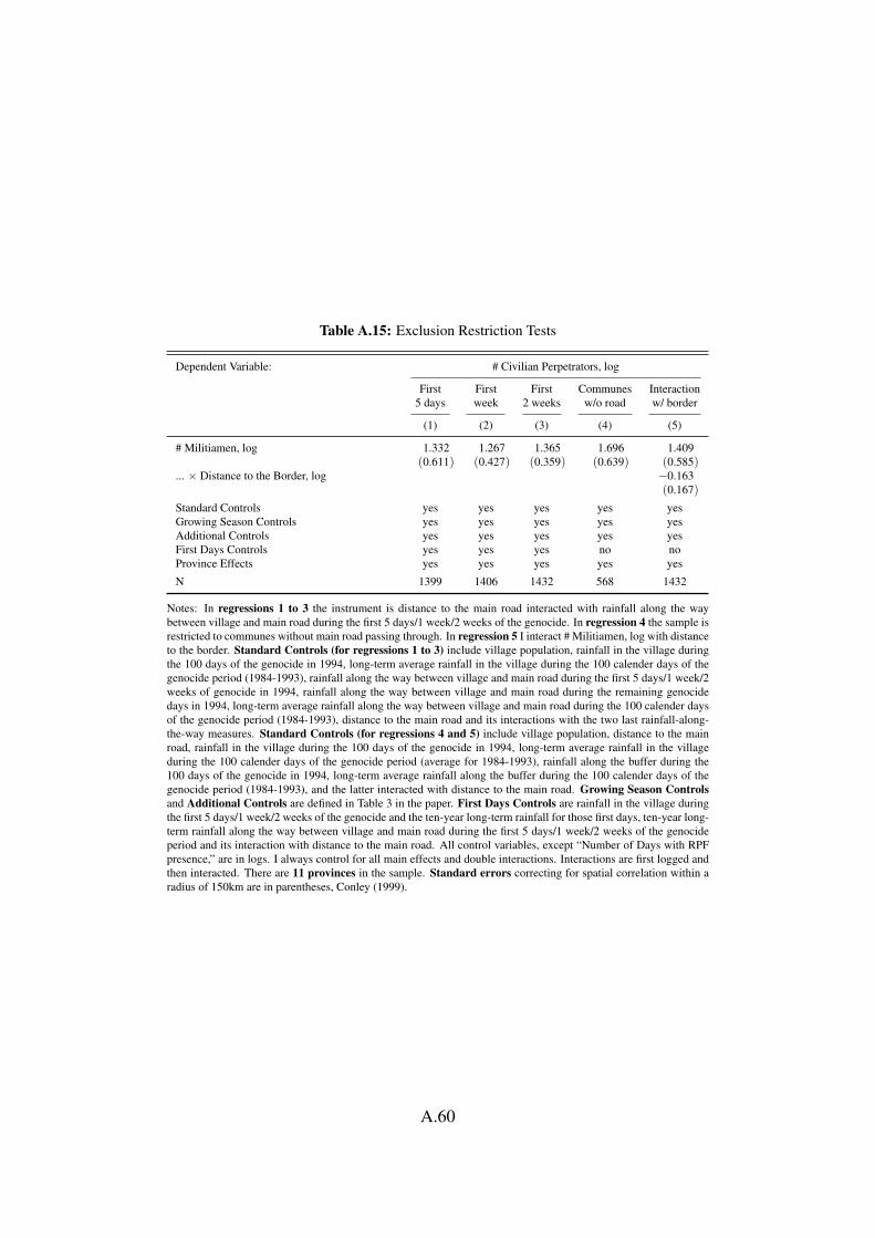
Table A.15: Exclusion Restriction Tests
Dependent Variable: # Civilian Perpetrators, log
First First First Communes Interaction5 days week 2 weeks w/o road w/ border
(1) (2) (3) (4) (5)
# Militiamen, log 1.332 1.267 1.365 1.696 1.409(0.611) (0.427) (0.359) (0.639) (0.585)
... × Distance to the Border, log −0.163(0.167)
Standard Controls yes yes yes yes yesGrowing Season Controls yes yes yes yes yesAdditional Controls yes yes yes yes yesFirst Days Controls yes yes yes no noProvince Effects yes yes yes yes yes
N 1399 1406 1432 568 1432
Notes: In regressions 1 to 3 the instrument is distance to the main road interacted with rainfall along the waybetween village and main road during the first 5 days/1 week/2 weeks of the genocide. In regression 4 the sample isrestricted to communes without main road passing through. In regression 5 I interact # Militiamen, log with distanceto the border. Standard Controls (for regressions 1 to 3) include village population, rainfall in the village duringthe 100 days of the genocide in 1994, long-term average rainfall in the village during the 100 calender days of thegenocide period (1984-1993), rainfall along the way between village and main road during the first 5 days/1 week/2weeks of genocide in 1994, rainfall along the way between village and main road during the remaining genocidedays in 1994, long-term average rainfall along the way between village and main road during the 100 calender daysof the genocide period (1984-1993), distance to the main road and its interactions with the two last rainfall-along-the-way measures. Standard Controls (for regressions 4 and 5) include village population, distance to the mainroad, rainfall in the village during the 100 days of the genocide in 1994, long-term average rainfall in the villageduring the 100 calender days of the genocide period (average for 1984-1993), rainfall along the buffer during the100 days of the genocide in 1994, long-term average rainfall along the buffer during the 100 calender days of thegenocide period (1984-1993), and the latter interacted with distance to the main road. Growing Season Controlsand Additional Controls are defined in Table 3 in the paper. First Days Controls are rainfall in the village duringthe first 5 days/1 week/2 weeks of the genocide and the ten-year long-term rainfall for those first days, ten-year long-term rainfall along the way between village and main road during the first 5 days/1 week/2 weeks of the genocideperiod and its interaction with distance to the main road. All control variables, except “Number of Days with RPFpresence,” are in logs. I always control for all main effects and double interactions. Interactions are first logged andthen interacted. There are 11 provinces in the sample. Standard errors correcting for spatial correlation within aradius of 150km are in parentheses, Conley (1999).
A.60
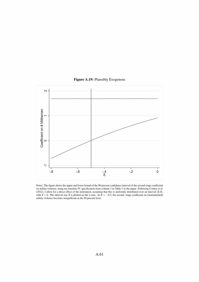
Figure A.19: Plausibly Exogenous
Notes: The figure shows the upper and lower bound of the 90 percent confidence interval of the second-stage coefficienton militia violence, using my baseline IV specification from column 3 in Table 3 in the paper. Following Conley et al.(2012), I allow for a direct effect of the instrument, assuming that this is uniformly distributed over an interval [δ ,0],with δ < 0. The interval size δ is plotted on the x-axis. At δ = −0.5, the second -stage coefficient on (instrumented)militia violence becomes insignificant at the 90 percent level.
A.61
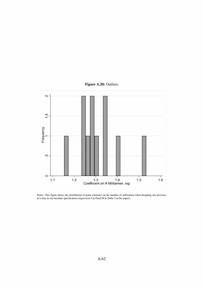
Figure A.20: Outliers
Notes: This figure shows the distribution of point estimates on the number of militiamen when dropping one provinceat a time in my baseline specification (regression 6 in Panel B in Table 3 in the paper).
A.62
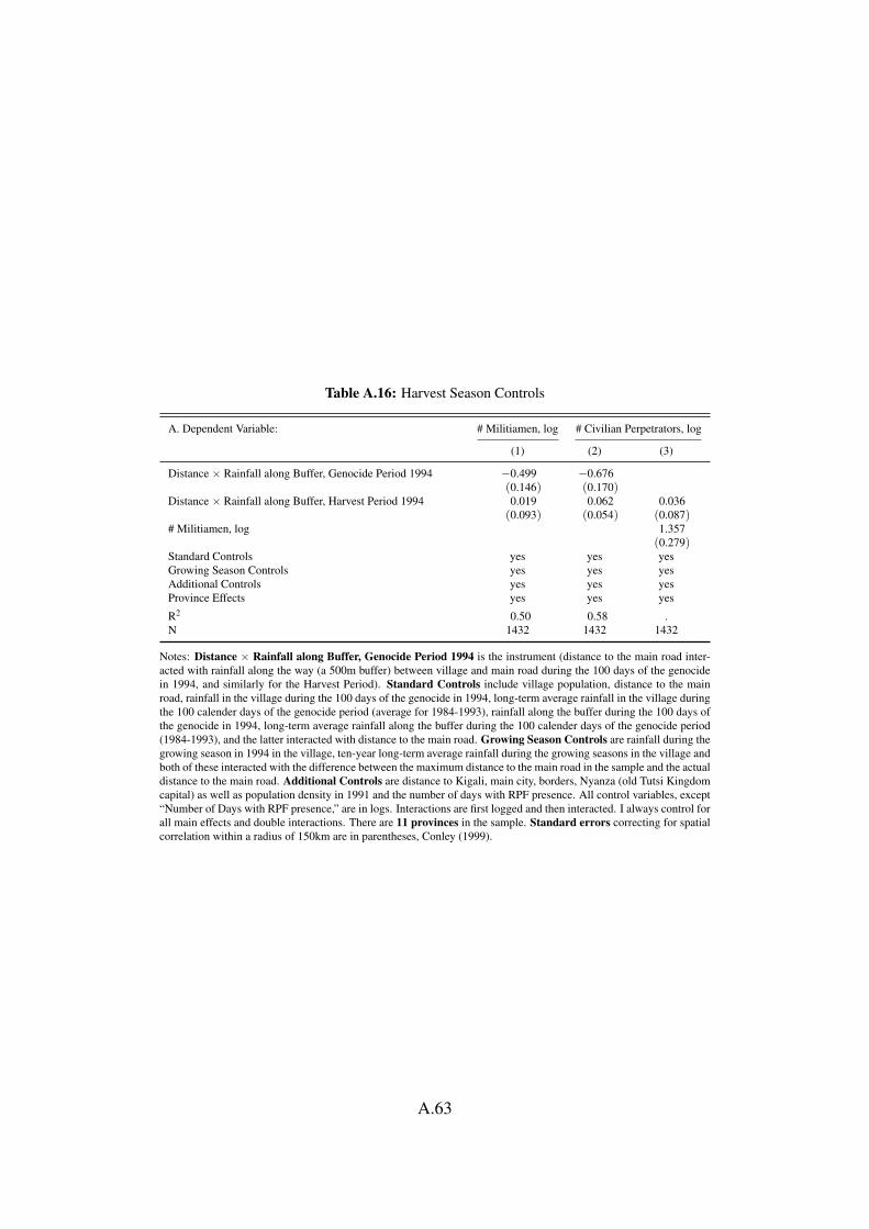
Table A.16: Harvest Season Controls
A. Dependent Variable: # Militiamen, log # Civilian Perpetrators, log
(1) (2) (3)
Distance × Rainfall along Buffer, Genocide Period 1994 −0.499 −0.676(0.146) (0.170)
Distance × Rainfall along Buffer, Harvest Period 1994 0.019 0.062 0.036(0.093) (0.054) (0.087)
# Militiamen, log 1.357(0.279)
Standard Controls yes yes yesGrowing Season Controls yes yes yesAdditional Controls yes yes yesProvince Effects yes yes yes
R2 0.50 0.58 .N 1432 1432 1432
Notes: Distance × Rainfall along Buffer, Genocide Period 1994 is the instrument (distance to the main road inter-acted with rainfall along the way (a 500m buffer) between village and main road during the 100 days of the genocidein 1994, and similarly for the Harvest Period). Standard Controls include village population, distance to the mainroad, rainfall in the village during the 100 days of the genocide in 1994, long-term average rainfall in the village duringthe 100 calender days of the genocide period (average for 1984-1993), rainfall along the buffer during the 100 days ofthe genocide in 1994, long-term average rainfall along the buffer during the 100 calender days of the genocide period(1984-1993), and the latter interacted with distance to the main road. Growing Season Controls are rainfall during thegrowing season in 1994 in the village, ten-year long-term average rainfall during the growing seasons in the village andboth of these interacted with the difference between the maximum distance to the main road in the sample and the actualdistance to the main road. Additional Controls are distance to Kigali, main city, borders, Nyanza (old Tutsi Kingdomcapital) as well as population density in 1991 and the number of days with RPF presence. All control variables, except“Number of Days with RPF presence,” are in logs. Interactions are first logged and then interacted. I always control forall main effects and double interactions. There are 11 provinces in the sample. Standard errors correcting for spatialcorrelation within a radius of 150km are in parentheses, Conley (1999).
A.63
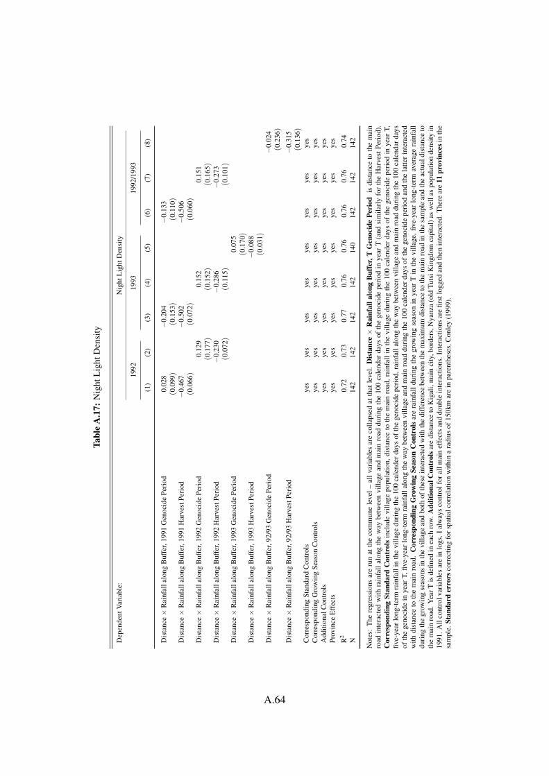
Tabl
eA
.17:
Nig
htL
ight
Den
sity
Dep
ende
ntV
aria
ble:
Nig
htL
ight
Den
sity
1992
1993
1992
/199
3
(1)
(2)
(3)
(4)
(5)
(6)
(7)
(8)
Dis
tanc
e×
Rai
nfal
lalo
ngB
uffe
r,19
91G
enoc
ide
Peri
od0.
028
−0.
204
−0.
133
(0.0
99)
(0.1
53)
(0.1
10)
Dis
tanc
e×
Rai
nfal
lalo
ngB
uffe
r,19
91H
arve
stPe
riod
−0.
467
−0.
502
−0.
506
(0.0
66)
(0.0
72)
(0.0
60)
Dis
tanc
e×
Rai
nfal
lalo
ngB
uffe
r,19
92G
enoc
ide
Peri
od0.
129
0.15
20.
151
(0.1
77)
(0.1
52)
(0.1
65)
Dis
tanc
e×
Rai
nfal
lalo
ngB
uffe
r,19
92H
arve
stPe
riod
−0.
230
−0.
286
−0.
273
(0.0
72)
(0.1
15)
(0.1
01)
Dis
tanc
e×
Rai
nfal
lalo
ngB
uffe
r,19
93G
enoc
ide
Peri
od0.
075
(0.1
70)
Dis
tanc
e×
Rai
nfal
lalo
ngB
uffe
r,19
93H
arve
stPe
riod
−0.
088
(0.0
31)
Dis
tanc
e×
Rai
nfal
lalo
ngB
uffe
r,92
/93
Gen
ocid
ePe
riod
−0.
024
(0.2
36)
Dis
tanc
e×
Rai
nfal
lalo
ngB
uffe
r,92
/93
Har
vest
Peri
od−
0.31
5(0
.136)
Cor
resp
ondi
ngSt
anda
rdC
ontr
ols
yes
yes
yes
yes
yes
yes
yes
yes
Cor
resp
ondi
ngG
row
ing
Seas
onC
ontr
ols
yes
yes
yes
yes
yes
yes
yes
yes
Add
ition
alC
ontr
ols
yes
yes
yes
yes
yes
yes
yes
yes
Prov
ince
Eff
ects
yes
yes
yes
yes
yes
yes
yes
yes
R2
0.72
0.73
0.77
0.76
0.76
0.76
0.76
0.74
N14
214
214
214
214
014
214
214
2
Not
es:
The
regr
essi
ons
are
run
atth
eco
mm
une
leve
l–al
lvar
iabl
esar
eco
llaps
edat
that
leve
l.D
ista
nce×
Rai
nfal
lalo
ngB
uffe
r,T
Gen
ocid
ePe
riod
isdi
stan
ceto
the
mai
nro
adin
tera
cted
with
rain
fall
alon
gth
ew
aybe
twee
nvi
llage
and
mai
nro
addu
ring
the
100
cale
ndar
days
ofth
ege
noci
depe
riod
inye
arT
(and
sim
ilarl
yfo
rth
eH
arve
stPe
riod
).C
orre
spon
ding
Stan
dard
Con
trol
sin
clud
evi
llage
popu
latio
n,di
stan
ceto
the
mai
nro
ad,r
ainf
alli
nth
evi
llage
duri
ngth
e10
0ca
lend
erda
ysof
the
geno
cide
peri
odin
year
T,fiv
e-ye
arlo
ng-t
erm
rain
fall
inth
evi
llage
duri
ngth
e10
0ca
lend
erda
ysof
the
geno
cide
peri
od,r
ainf
alla
long
the
way
betw
een
villa
gean
dm
ain
road
duri
ngth
e10
0ca
lend
arda
ysof
the
geno
cide
inye
arT,
five-
year
long
-ter
mra
infa
llal
ong
the
way
betw
een
villa
gean
dm
ain
road
duri
ngth
e10
0ca
lend
erda
ysof
the
geno
cide
peri
odan
dth
ela
tter
inte
ract
edw
ithdi
stan
ceto
the
mai
nro
ad.
Cor
resp
ondi
ngG
row
ing
Seas
onC
ontr
ols
are
rain
fall
duri
ngth
egr
owin
gse
ason
inye
arT
inth
evi
llage
,five
-yea
rlo
ng-t
erm
aver
age
rain
fall
duri
ngth
egr
owin
gse
ason
sin
the
villa
gean
dbo
thof
thes
ein
tera
cted
with
the
diff
eren
cebe
twee
nth
em
axim
umdi
stan
ceto
the
mai
nro
adin
the
sam
ple
and
the
actu
aldi
stan
ceto
the
mai
nro
ad.Y
earT
isde
fined
inea
chro
w.A
dditi
onal
Con
trol
sare
dist
ance
toK
igal
i,m
ain
city
,bor
ders
,Nya
nza
(old
Tuts
iKin
gdom
capi
tal)
asw
ella
spo
pula
tion
dens
ityin
1991
.All
cont
rolv
aria
bles
are
inlo
gs.I
alw
ays
cont
rolf
oral
lmai
nef
fect
san
ddo
uble
inte
ract
ions
.Int
erac
tions
are
first
logg
edan
dth
enin
tera
cted
.The
rear
e11
prov
ince
sin
the
sam
ple.
Stan
dard
erro
rsco
rrec
ting
fors
patia
lcor
rela
tion
with
ina
radi
usof
150k
mar
ein
pare
nthe
ses,
Con
ley
(199
9).
A.64
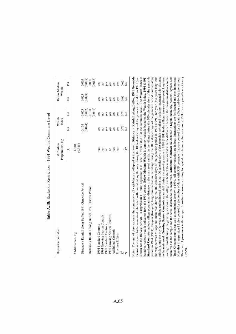
Tabl
eA
.18:
Exc
lusi
onR
estr
ictio
n–
1991
Wea
lth,C
omm
une
Lev
el
Dep
ende
ntV
aria
ble:
#C
ivili
anW
ealth
Bel
owM
edia
nPe
rpet
rato
rs,l
ogIn
dex
Wea
lth
(1)
(2)
(3)
(4)
(5)
#M
ilitia
men
,log
1.38
0(0
.345)
Dis
tanc
ex
Rai
nfal
lalo
ngB
uffe
r,19
91G
enoc
ide
Peri
od−
0.17
4−
0.05
30.
025
0.00
5(0
.074)
(0.0
72)
(0.0
28)
(0.0
28)
Dis
tanc
ex
Rai
nfal
lalo
ngB
uffe
r,19
91H
arve
stPe
riod
−0.
198
0.03
0(0
.041)
(0.0
18)
1994
Stan
dard
Con
trol
sye
sye
sye
sye
sye
s19
94G
row
ing
Seas
onC
ontr
ols
yes
nono
nono
1991
Stan
dard
Con
trol
sno
yes
yes
yes
yes
1991
Gro
win
gSe
ason
Con
trol
sno
yes
yes
yes
yes
Add
ition
alC
ontr
ols
yes
yes
yes
yes
yes
Prov
ince
Eff
ects
yes
yes
yes
yes
yes
R2
.0.
730.
740.
620.
62N
142
142
142
142
142
Not
es:
The
unit
ofob
serv
atio
nis
the
com
mun
e–
allv
aria
bles
are
colla
psed
atth
atle
vel.
Dis
tanc
e×
Rai
nfal
lalo
ngB
uffe
r,19
91G
enoc
ide
Peri
odis
dist
ance
toth
em
ain
road
inte
ract
edw
ithra
infa
llal
ong
the
way
duri
ngth
e10
0ca
lend
erda
ysof
the
geno
cide
peri
odfr
om19
91(a
ndsi
mila
rfo
rth
eH
arve
stpe
riod
).In
regr
essi
on1
Ire
run
regr
essi
on6
inPa
nel
Bfr
omTa
ble
3at
the
com
mun
ele
vel.
The
Wea
lthIn
dex
isba
sed
onva
riou
sw
ealth
indi
cato
rsfr
omth
e19
91ce
nsus
.Bel
owM
edia
nW
ealth
isdu
mm
yva
riab
leba
sed
onth
eW
ealth
Inde
x.19
94(1
991)
Stan
dard
Con
trol
sin
clud
evi
llage
popu
latio
n,di
stan
ceto
the
mai
nro
ad,r
ainf
alli
nth
evi
llage
duri
ngth
e10
0ca
lend
erda
ysof
the
geno
cide
peri
odin
1994
(199
1),t
en-y
ear(
five-
year
)lon
g-te
rmra
infa
llin
the
villa
gedu
ring
the
100
cale
nder
days
ofth
ege
noci
depe
riod
,rai
nfal
lalo
ngth
ew
aybe
twee
nvi
llage
and
mai
nro
addu
ring
the
100
cale
nder
days
ofth
ege
noci
depe
riod
in19
94(1
991)
,ten
-yea
r(fi
ve-y
ear)
long
-ter
mra
infa
llal
ong
the
way
betw
een
villa
gean
dm
ain
road
duri
ngth
e10
0ca
lend
erda
ysof
the
geno
cide
peri
odan
dth
ela
tteri
nter
acte
dw
ithdi
stan
ceto
the
mai
nro
ad.G
row
ing
Seas
onC
ontr
olsa
rera
infa
lldu
ring
the
grow
ing
seas
onin
1994
(199
1)in
the
villa
ge,t
en-y
ear(
five-
year
)lon
g-te
rmav
erag
era
infa
lldu
ring
the
grow
ing
seas
ons
inth
evi
llage
and
both
ofth
ese
inte
ract
edw
ithth
edi
ffer
ence
betw
een
the
max
imum
dist
ance
toth
em
ain
road
inth
esa
mpl
ean
dth
eac
tual
dist
ance
toth
em
ain
road
.Add
ition
alC
ontr
olsa
redi
stan
ceto
Kig
ali,
mai
nci
ty,b
orde
rs,N
yanz
a(o
ldTu
tsiK
ingd
omca
pita
l)as
wel
las
popu
latio
nde
nsity
in19
91.A
llco
ntro
lvar
iabl
esar
ein
logs
.Int
erac
tions
are
first
logg
edan
dth
enin
tera
cted
.N
ote
that
inre
gres
sion
1Ia
lso
cont
rolf
orth
enu
mbe
rofd
ays
with
RPF
pres
ence
.Ial
way
sco
ntro
lfor
allm
ain
effe
cts
and
doub
lein
tera
ctio
ns.
The
rear
e11
prov
ince
sin
the
sam
ple.
Stan
dard
erro
rsco
rrec
ting
fors
patia
lcor
rela
tion
with
ina
radi
usof
150k
mar
ein
pare
nthe
ses,
Con
ley
(199
9).
A.65
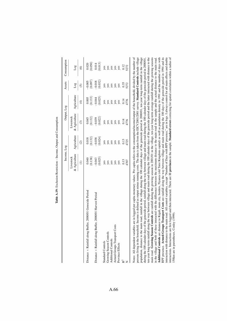
Tabl
eA
.19:
Exc
lusi
onR
estr
ictio
n–
Inco
me,
Out
puta
ndC
onsu
mpt
ion
Inco
me,
Log
Out
put,
Log
Ass
ets
Con
sum
ptio
n
Liv
esto
ckL
ives
tock
&A
gric
ultu
reA
gric
ultu
re&
Agr
icul
ture
Agr
icul
ture
Log
Log
(1)
(2)
(3)
(4)
(5)
(6)
Dis
tanc
e×
Rai
nfal
lalo
ngB
uffe
r,20
00/0
1G
enoc
ide
Peri
od0.
040
0.01
80.
045
0.00
5−
0.00
50.
020
(0.1
38)
(0.1
32)
(0.1
32)
(0.1
33)
(0.0
97)
(0.0
50)
Dis
tanc
e×
Rai
nfal
lalo
ngB
uffe
r,20
00/0
1H
arve
stPe
riod
−0.
043
−0.
038
−0.
039
−0.
044
−0.
018
0.01
4(0
.025)
(0.0
24)
(0.0
22)
(0.0
25)
(0.0
32)
(0.0
13)
Stan
dard
Con
trol
sye
sye
sye
sye
sye
sye
sG
row
ing
Seas
onC
ontr
ols
yes
yes
yes
yes
yes
yes
Add
ition
alC
ontr
ols
yes
yes
yes
yes
yes
yes
Arm
ed-G
roup
sTr
ansp
ortC
osts
yes
yes
yes
yes
yes
yes
Prov
ince
Eff
ects
yes
yes
yes
yes
yes
yes
R2
0.13
0.13
0.14
0.14
0.35
0.12
N47
0747
2547
7647
7652
7252
72
Not
es:
All
depe
nden
tvar
iabl
esar
ein
logg
edpe
rcap
itam
onet
ary
valu
es.P
erca
pita
refe
rsto
the
cons
umpt
ion/
inco
me/
outp
utof
the
hous
ehol
d,di
vide
dby
the
num
bero
fpe
rson
sliv
ing
inth
eho
useh
old.
Inco
me
isde
fined
asou
tput
min
usru
nnin
gco
sts.
The
data
ista
ken
from
the
EIC
V20
01/2
001
surv
ey.S
tand
ard
Con
trol
sinc
lude
villa
gepo
pula
tion,
dist
ance
toth
em
ain
road
,rai
nfal
lin
the
villa
gedu
ring
the
100
cale
nder
days
ofth
ege
noci
depe
riod
in20
00/0
1,te
n-ye
arlo
ng-t
erm
rain
fall
inth
evi
llage
duri
ngth
e10
0ca
lend
erda
ysof
the
geno
cide
peri
od,r
ainf
alla
long
the
way
betw
een
villa
gean
dm
ain
road
duri
ngth
e10
0ca
lend
erda
ysof
the
geno
cide
peri
odin
2000
/01,
ten-
year
long
-ter
mra
infa
llal
ong
the
way
betw
een
villa
gean
dm
ain
road
duri
ngth
e10
0ca
lend
erda
ysof
the
geno
cide
peri
odan
dth
ela
tteri
nter
acte
dw
ithdi
stan
ceto
the
mai
nro
ad.
Gro
win
gSe
ason
Con
trol
sar
era
infa
lldu
ring
the
grow
ing
seas
onin
2001
/01
inth
evi
llage
,ten
-yea
rlo
ng-t
erm
aver
age
rain
fall
duri
ngth
egr
owin
gse
ason
sin
the
villa
gean
dbo
thof
thes
ein
tera
cted
with
the
diff
eren
cebe
twee
nth
em
axim
umdi
stan
ceto
the
mai
nro
adin
the
sam
ple
and
the
actu
aldi
stan
ceto
the
mai
nro
ad.
Add
ition
alC
ontr
ols
are
dist
ance
toK
igal
i,m
ain
city
,bor
ders
,Nya
nza
(old
Tuts
iKin
gdom
capi
tal)
asw
ella
spo
pula
tion
dens
ityin
1991
and
the
num
ber
ofda
ysw
ithR
PFpr
esen
ce.
Arm
ed-G
roup
sTr
ansp
ortC
osts
are
rain
fall
alon
gth
ew
aybe
twee
nvi
llage
and
mai
nro
addu
ring
the
100
days
ofth
ege
noci
depe
riod
in19
94an
dits
inte
ract
ion
with
dist
ance
toth
em
ain
road
.All
cont
rolv
aria
bles
,exc
ept“
Num
bero
fDay
sw
ithR
PFpr
esen
ce,”
are
inlo
gs.I
alw
ays
cont
rolf
oral
lmai
nef
fect
san
ddo
uble
inte
ract
ions
.Int
erac
tions
are
first
logg
edan
dth
enin
tera
cted
.The
rear
e11
prov
ince
sin
the
sam
ple.
Stan
dard
erro
rsco
rrec
ting
fors
patia
lcor
rela
tion
with
ina
radi
usof
150k
mar
ein
pare
nthe
ses,
Con
ley
(199
9).
A.66
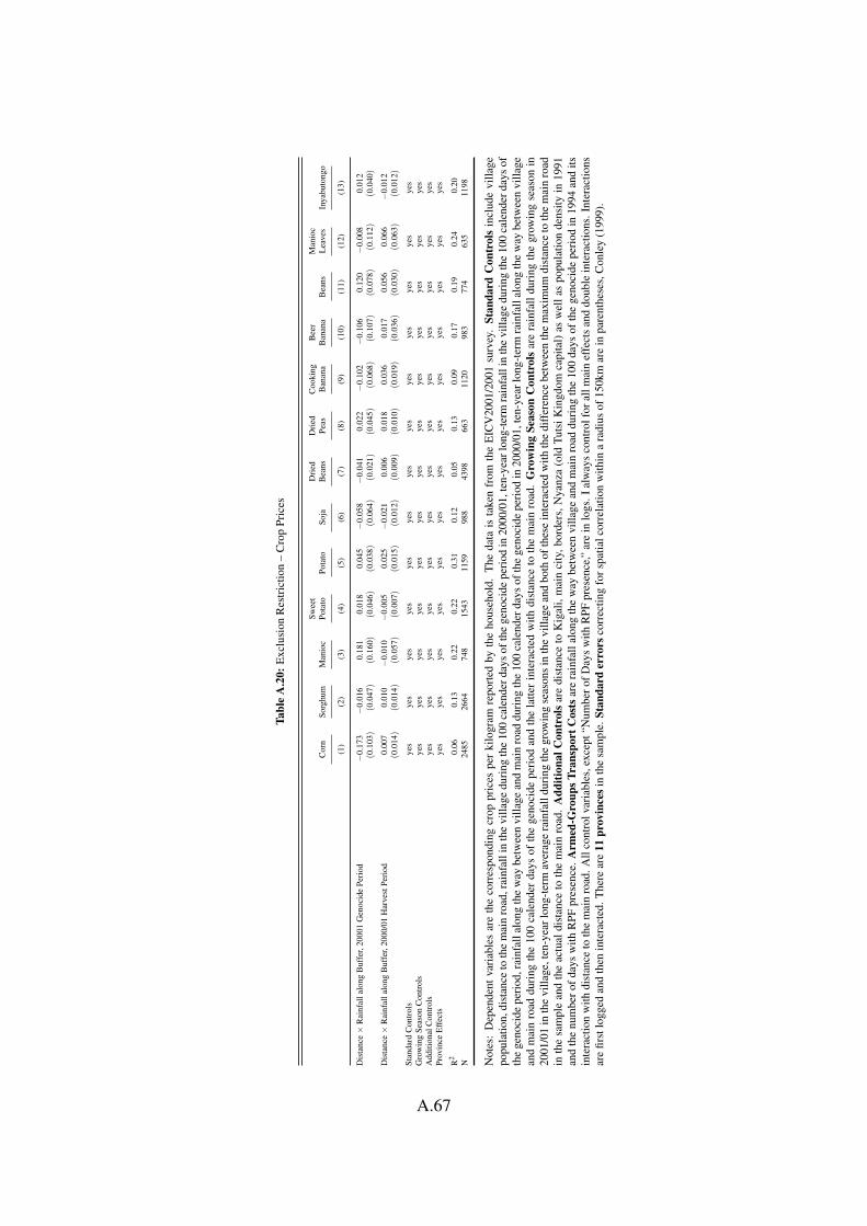
Tabl
eA
.20:
Exc
lusi
onR
estr
ictio
n–
Cro
pPr
ices
Swee
tD
ried
Dri
edC
ooki
ngB
eer
Man
ioc
Cor
nSo
rghu
mM
anio
cPo
tato
Pota
toSo
jaB
eans
Peas
Ban
ana
Ban
ana
Bea
nsL
eave
sIn
yabu
tong
o
(1)
(2)
(3)
(4)
(5)
(6)
(7)
(8)
(9)
(10)
(11)
(12)
(13)
Dis
tanc
e×
Rai
nfal
lalo
ngB
uffe
r,20
001
Gen
ocid
ePe
riod
−0.
173
−0.
016
0.18
10.
018
0.04
5−
0.05
8−
0.04
10.
022
−0.
102
−0.
106
0.12
0−
0.00
80.
012
(0.1
03)
(0.0
47)
(0.1
60)
(0.0
46)
(0.0
38)
(0.0
64)
(0.0
21)
(0.0
45)
(0.0
68)
(0.1
07)
(0.0
78)
(0.1
12)
(0.0
40)
Dis
tanc
e×
Rai
nfal
lalo
ngB
uffe
r,20
00/0
1H
arve
stPe
riod
0.00
70.
010
−0.
010
−0.
005
0.02
5−
0.02
10.
006
0.01
80.
036
0.01
70.
056
0.06
6−
0.01
2(0
.014)
(0.0
14)
(0.0
57)
(0.0
07)
(0.0
15)
(0.0
12)
(0.0
09)
(0.0
10)
(0.0
19)
(0.0
36)
(0.0
30)
(0.0
63)
(0.0
12)
Stan
dard
Con
trol
sye
sye
sye
sye
sye
sye
sye
sye
sye
sye
sye
sye
sye
sG
row
ing
Seas
onC
ontr
ols
yes
yes
yes
yes
yes
yes
yes
yes
yes
yes
yes
yes
yes
Add
ition
alC
ontr
ols
yes
yes
yes
yes
yes
yes
yes
yes
yes
yes
yes
yes
yes
Prov
ince
Eff
ects
yes
yes
yes
yes
yes
yes
yes
yes
yes
yes
yes
yes
yes
R2
0.06
0.13
0.22
0.22
0.31
0.12
0.05
0.13
0.09
0.17
0.19
0.24
0.20
N24
8526
6474
815
4311
5998
843
9866
311
2098
377
463
511
98
Not
es:
Dep
ende
ntva
riab
les
are
the
corr
espo
ndin
gcr
oppr
ices
per
kilo
gram
repo
rted
byth
eho
useh
old.
The
data
ista
ken
from
the
EIC
V20
01/2
001
surv
ey.
Stan
dard
Con
trol
sin
clud
evi
llage
popu
latio
n,di
stan
ceto
the
mai
nro
ad,r
ainf
alli
nth
evi
llage
duri
ngth
e10
0ca
lend
erda
ysof
the
geno
cide
peri
odin
2000
/01,
ten-
year
long
-ter
mra
infa
llin
the
villa
gedu
ring
the
100
cale
nder
days
ofth
ege
noci
depe
riod
,rai
nfal
lalo
ngth
ew
aybe
twee
nvi
llage
and
mai
nro
addu
ring
the
100
cale
nder
days
ofth
ege
noci
depe
riod
in20
00/0
1,te
n-ye
arlo
ng-t
erm
rain
fall
alon
gth
ew
aybe
twee
nvi
llage
and
mai
nro
addu
ring
the
100
cale
nder
days
ofth
ege
noci
depe
riod
and
the
latte
rin
tera
cted
with
dist
ance
toth
em
ain
road
.G
row
ing
Seas
onC
ontr
ols
are
rain
fall
duri
ngth
egr
owin
gse
ason
in20
01/0
1in
the
villa
ge,t
en-y
earl
ong-
term
aver
age
rain
fall
duri
ngth
egr
owin
gse
ason
sin
the
villa
gean
dbo
thof
thes
ein
tera
cted
with
the
diff
eren
cebe
twee
nth
em
axim
umdi
stan
ceto
the
mai
nro
adin
the
sam
ple
and
the
actu
aldi
stan
ceto
the
mai
nro
ad.
Add
ition
alC
ontr
ols
are
dist
ance
toK
igal
i,m
ain
city
,bor
ders
,Nya
nza
(old
Tuts
iKin
gdom
capi
tal)
asw
ella
spo
pula
tion
dens
ityin
1991
and
the
num
bero
fday
sw
ithR
PFpr
esen
ce.A
rmed
-Gro
upsT
rans
port
Cos
tsar
era
infa
llal
ong
the
way
betw
een
villa
gean
dm
ain
road
duri
ngth
e10
0da
ysof
the
geno
cide
peri
odin
1994
and
itsin
tera
ctio
nw
ithdi
stan
ceto
the
mai
nro
ad.A
llco
ntro
lvar
iabl
es,e
xcep
t“N
umbe
rofD
ays
with
RPF
pres
ence
,”ar
ein
logs
.Ial
way
sco
ntro
lfor
allm
ain
effe
cts
and
doub
lein
tera
ctio
ns.I
nter
actio
nsar
efir
stlo
gged
and
then
inte
ract
ed.T
here
are
11pr
ovin
cesi
nth
esa
mpl
e.St
anda
rder
rors
corr
ectin
gfo
rspa
tialc
orre
latio
nw
ithin
ara
dius
of15
0km
are
inpa
rent
hese
s,C
onle
y(1
999)
.
A.67
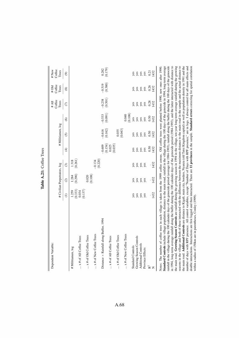
Tabl
eA
.21:
Cof
fee
Tree
s
Dep
ende
ntV
aria
ble:
#A
ll#
Old
#N
ewC
offe
eC
offe
eC
offe
e#
Civ
ilian
Perp
etra
tors
,log
#M
ilitia
men
,log
Tree
sTr
ees
Tree
s
(1)
(2)
(3)
(4)
(5)
(6)
(7)
(8)
(9)
#M
ilitia
men
,log
1.25
91.
284
1.31
8(0
.333)
(0.2
90)
(0.2
61)
...x
#of
All
Cof
fee
Tree
s0.
034
(0.1
37)
...x
#of
Old
Cof
fee
Tree
s0.
020
(0.1
08)
...x
#of
New
Cof
fee
Tree
s−
0.13
4(0
.220)
Dis
tanc
e×
Rai
nfal
lalo
ngB
uffe
r,19
94−
0.60
9−
0.61
6−
0.53
3−
0.23
8−
0.51
90.
282
(0.1
54)
(0.1
62)
(0.0
91)
(0.5
01)
(0.3
80)
(0.1
79)
...x
#of
All
Cof
fee
Tree
s0.
025
(0.0
35)
...x
#of
Old
Cof
fee
Tree
s0.
035
(0.0
43)
...x
#of
New
Cof
fee
Tree
s0.
040
(0.1
08)
Stan
dard
Con
trol
sye
sye
sye
sye
sye
sye
sye
sye
sye
sG
row
ing
Seas
onC
ontr
ols
yes
yes
yes
yes
yes
yes
yes
yes
yes
Add
ition
alC
ontr
ols
yes
yes
yes
yes
yes
yes
yes
yes
yes
Prov
ince
Eff
ects
yes
yes
yes
yes
yes
yes
yes
yes
yes
R2
..
.0.
500.
500.
500.
280.
260.
21N
1432
1432
1432
1432
1432
1432
1432
1432
1432
Not
es:
The
num
ber
ofco
ffee
tree
sin
each
villa
geis
take
nfr
omth
e19
99co
ffee
cens
us.
Old
coff
eetr
ees
wer
epl
ante
dbe
fore
1990
,ne
won
esaf
ter
1990
.St
anda
rdC
ontr
ols
incl
ude
villa
gepo
pula
tion,
dist
ance
toth
em
ain
road
,rai
nfal
lin
the
villa
gedu
ring
the
100
days
ofth
ege
noci
dein
1994
,lon
g-te
rmav
erag
era
infa
llin
the
villa
gedu
ring
the
100
cale
nder
days
ofth
ege
noci
depe
riod
(ave
rage
for1
984-
1993
),ra
infa
llal
ong
the
buff
erdu
ring
the
100
days
ofth
ege
noci
dein
1994
,lon
g-te
rmav
erag
era
infa
llal
ong
the
buff
erdu
ring
the
100
cale
nder
days
ofth
ege
noci
depe
riod
(198
4-19
93),
and
the
latte
rin
tera
cted
with
dist
ance
toth
em
ain
road
.G
row
ing
Seas
onC
ontr
ols
are
rain
fall
duri
ngth
egr
owin
gse
ason
in19
94in
the
villa
ge,t
en-y
ear
long
-ter
mav
erag
era
infa
lldu
ring
the
grow
ing
seas
ons
inth
evi
llage
and
both
ofth
ese
inte
ract
edw
ithth
edi
ffer
ence
betw
een
the
max
imum
dist
ance
toth
em
ain
road
inth
esa
mpl
ean
dth
eac
tual
dist
ance
toth
em
ain
road
.Add
ition
alC
ontr
olsa
redi
stan
ceto
Kig
ali,
mai
nci
ty,b
orde
rs,N
yanz
a(o
ldTu
tsiK
ingd
omca
pita
l)as
wel
las
popu
latio
nde
nsity
in19
91an
dth
enu
mbe
rof
days
with
RPF
pres
ence
.A
llco
ntro
lvar
iabl
es,e
xcep
t“N
umbe
rof
Day
sw
ithR
PFpr
esen
ce,”
are
inlo
gs.
Ial
way
sco
ntro
lfor
allm
ain
effe
cts
and
doub
lein
tera
ctio
ns.
Inte
ract
ions
are
first
logg
edan
dth
enin
tera
cted
.T
here
are
11pr
ovin
ces
inth
esa
mpl
e.St
anda
rder
rors
corr
ectin
gfo
rsp
atia
lcor
rela
tion
with
ina
radi
usof
150k
mar
ein
pare
nthe
ses,
Con
ley
(199
9).
A.68

Tabl
eA
.22:
Cof
fee
Mill
s
Dep
ende
ntV
aria
ble:
#C
ivili
anPe
rpet
rato
rs,l
og#
Mili
tiam
en,l
og
No
Cof
fee
Mill
with
in:
x=
0km
x=
10km
x=
20km
x=
0km
x=
10km
x=
20km
x=
0km
x=
10km
x=
20km
(1)
(2)
(3)
(4)
(5)
(6)
(7)
(8)
(9)
#M
ilitia
men
,log
1.29
11.
274
1.42
21.
280
1.27
81.
322
(0.2
52)
(0.2
50)
(0.2
43)
(0.2
54)
(0.2
59)
(0.2
78)
...x
Cof
fee
Mill
with
inx
km−
0.41
3−
0.30
4−
0.42
4(0
.295)
(0.2
92)
(0.4
44)
Dis
tanc
e×
Rai
nfal
lalo
ngB
uffe
r,19
94−
0.56
5−
0.55
4−
0.55
7(0
.100)
(0.1
01)
(0.1
14)
...x
Cof
fee
Mill
with
inx
km−
0.13
4−
0.22
6−
0.13
2(0
.152)
(0.1
39)
(0.1
87)
Stan
dard
Con
trol
sye
sye
sye
sye
sye
sye
sye
sye
sye
sG
row
ing
Seas
onC
ontr
ols
yes
yes
yes
yes
yes
yes
yes
yes
yes
Add
ition
alC
ontr
ols
yes
yes
yes
yes
yes
yes
yes
yes
yes
Prov
ince
Eff
ects
yes
yes
yes
yes
yes
yes
yes
yes
yes
R2
..
..
..
0.50
0.50
0.50
N11
9711
6596
814
3114
3114
3114
3114
3114
31
Not
es:T
helo
catio
nof
coff
eem
ills
ista
ken
from
Gua
riso
and
Ver
poor
ten
(201
8).I
nre
gres
sion
s1to
3Id
rop
allv
illag
esw
ithin
xki
lom
eter
sof
aco
ffee
mill
,the
cuto
ffdi
stan
ceis
give
nin
the
colu
mn
head
er(0
mea
nsno
mill
inth
evi
llage
itsel
f).R
egre
ssio
ns4
to9
cont
rolf
orva
riou
sco
ffee
mill
inte
ract
ions
.Sta
ndar
dC
ontr
ols
incl
ude
villa
gepo
pula
tion,
dist
ance
toth
em
ain
road
,rai
nfal
lin
the
villa
gedu
ring
the
100
days
ofth
ege
noci
dein
1994
,lon
g-te
rmav
erag
era
infa
llin
the
villa
gedu
ring
the
100
cale
nder
days
ofth
ege
noci
depe
riod
(ave
rage
for1
984-
1993
),ra
infa
llal
ong
the
buff
erdu
ring
the
100
days
ofth
ege
noci
dein
1994
,lon
g-te
rmav
erag
era
infa
llal
ong
the
buff
erdu
ring
the
100
cale
nder
days
ofth
ege
noci
depe
riod
(198
4-19
93),
and
the
latte
rint
erac
ted
with
dist
ance
toth
em
ain
road
.Gro
win
gSe
ason
Con
trol
sare
rain
fall
duri
ngth
egr
owin
gse
ason
in19
94in
the
villa
ge,
ten-
year
long
-ter
mav
erag
era
infa
lldu
ring
the
grow
ing
seas
ons
inth
evi
llage
and
both
ofth
ese
inte
ract
edw
ithth
edi
ffer
ence
betw
een
the
max
imum
dist
ance
toth
em
ain
road
inth
esa
mpl
ean
dth
eac
tual
dist
ance
toth
em
ain
road
.A
dditi
onal
Con
trol
sar
edi
stan
ceto
Kig
ali,
mai
nci
ty,b
orde
rs,N
yanz
a(o
ldTu
tsiK
ingd
omca
pita
l)as
wel
las
popu
latio
nde
nsity
in19
91an
dth
enu
mbe
rof
days
with
RPF
pres
ence
.A
llco
ntro
lvar
iabl
es,e
xcep
t“N
umbe
rof
Day
sw
ithR
PFpr
esen
ce,”
are
inlo
gs.
Ial
way
sco
ntro
lfor
allm
ain
effe
cts
and
doub
lein
tera
ctio
ns.I
nter
actio
nsar
efir
stlo
gged
and
then
inte
ract
ed.T
here
are
11pr
ovin
cesi
nth
esa
mpl
e.St
anda
rder
rors
corr
ectin
gfo
rspa
tialc
orre
latio
nw
ithin
ara
dius
of15
0km
are
inpa
rent
hese
s,C
onle
y(1
999)
.
A.69
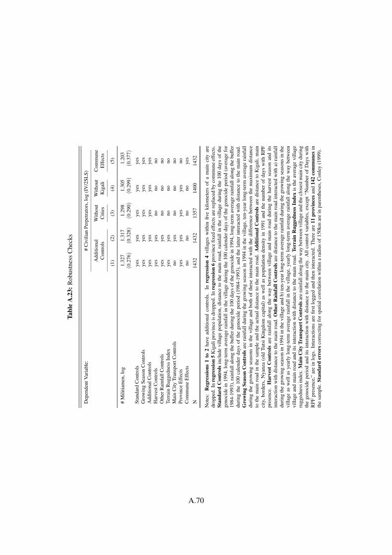
Tabl
eA
.23:
Rob
ustn
ess
Che
cks
Dep
ende
ntV
aria
ble:
#C
ivili
anPe
rpet
rato
rs,l
og(I
V/2
SLS)
Add
ition
alW
ithou
tW
ithou
tC
omm
une
Con
trol
sC
ities
Kig
ali
Eff
ects
(1)
(2)
(3)
(4)
(5)
#M
ilitia
men
,log
1.32
71.
317
1.29
81.
305
1.20
3(0
.276)
(0.3
28)
(0.2
90)
(0.2
99)
(0.3
77)
Stan
dard
Con
trol
sye
sye
sye
sye
sye
sG
row
ing
Seas
onC
ontr
ols
yes
yes
yes
yes
yes
Add
ition
alC
ontr
ols
yes
yes
yes
yes
yes
Har
vest
Con
trol
sye
sye
sno
nono
Oth
erR
ainf
allC
ontr
ols
yes
yes
nono
noTe
rrai
nR
ugge
dnes
sIn
dex
yes
yes
nono
noM
ain
City
Tran
spor
tCon
trol
sno
yes
nono
noPr
ovin
ceE
ffec
tsye
sye
sye
sye
sno
Com
mun
eE
ffec
tsno
nono
noye
s
N14
3214
3213
5714
0014
32
Not
es:
Reg
ress
ions
1to
2ha
vead
ditio
nal
cont
rols
.In
regr
essi
on4
villa
ges
with
infiv
eki
lom
eter
sof
am
ain
city
are
drop
ped.
Inre
gres
sion
5K
igal
ipro
vinc
eis
drop
ped.
Inre
gres
sion
6pr
ovin
cefix
edef
fect
sar
ere
plac
edby
com
mun
eef
fect
s.St
anda
rdC
ontr
ols
incl
ude
villa
gepo
pula
tion,
dist
ance
toth
em
ain
road
,rai
nfal
lin
the
villa
gedu
ring
the
100
days
ofth
ege
noci
dein
1994
,lon
g-te
rmav
erag
era
infa
llin
the
villa
gedu
ring
the
100
cale
nder
days
ofth
ege
noci
depe
riod
(ave
rage
for
1984
-199
3),r
ainf
alla
long
the
buff
erdu
ring
the
100
days
ofth
ege
noci
dein
1994
,lon
g-te
rmav
erag
era
infa
llal
ong
the
buff
erdu
ring
the
100
cale
nder
days
ofth
ege
noci
depe
riod
(198
4-19
93),
and
the
latte
rin
tera
cted
with
dist
ance
toth
em
ain
road
.G
row
ing
Seas
onC
ontr
ols
are
rain
fall
duri
ngth
egr
owin
gse
ason
in19
94in
the
villa
ge,t
en-y
earl
ong-
term
aver
age
rain
fall
duri
ngth
egr
owin
gse
ason
sin
the
villa
gean
dbo
thof
thes
ein
tera
cted
with
the
diff
eren
cebe
twee
nth
em
axim
umdi
stan
ceto
the
mai
nro
adin
the
sam
ple
and
the
actu
aldi
stan
ceto
the
mai
nro
ad.
Add
ition
alC
ontr
ols
are
dist
ance
toK
igal
i,m
ain
city
,bor
ders
,Nya
nza
(old
Tuts
iKin
gdom
capi
tal)
asw
ella
spo
pula
tion
dens
ityin
1991
and
the
num
ber
ofda
ysw
ithR
PFpr
esen
ce.
Har
vest
Con
trol
sar
era
infa
llal
ong
the
way
betw
een
villa
gean
dm
ain
road
duri
ngth
eha
rves
tse
ason
and
itsin
tera
ctio
nw
ithdi
stan
ceto
the
mai
nro
ad.O
ther
Rai
nfal
lCon
trol
sar
edi
stan
ceto
the
mai
nro
adin
tera
cted
with
a)ra
infa
lldu
ring
the
grow
ing
seas
onin
1994
inth
evi
llage
and
b)te
n-ye
arlo
ng-t
erm
aver
age
rain
fall
duri
ngth
egr
owin
gse
ason
sin
the
villa
geas
wel
las
year
lylo
ng-t
erm
aver
age
rain
fall
inth
evi
llage
,yea
rly
long
-ter
mav
erag
era
infa
llal
ong
the
way
betw
een
villa
gean
dm
ain
road
and
itsin
tera
ctio
nw
ithdi
stan
ceto
the
mai
nro
ad.
Terr
ain
Rug
gedn
ess
Inde
xis
the
aver
age
villa
geru
gged
ness
inde
x.M
ain
City
Tran
spor
tCon
trol
sare
rain
fall
alon
gth
ew
aybe
twee
nvi
llage
and
the
clos
estm
ain
city
duri
ngth
ege
noci
depe
riod
and
itsin
tera
ctio
nw
ithdi
stan
ceto
the
mai
nci
ty.
All
cont
rolv
aria
bles
,exc
ept“
Num
ber
ofD
ays
with
RPF
pres
ence
,”ar
ein
logs
.In
tera
ctio
nsar
efir
stlo
gged
and
then
inte
ract
ed.
The
rear
e11
prov
ince
san
d14
2co
mm
unes
inth
esa
mpl
e.St
anda
rder
rors
corr
ectin
gfo
rspa
tialc
orre
latio
nw
ithin
ara
dius
of15
0km
are
inpa
rent
hese
s,C
onle
y(1
999)
.
A.70

Tabl
eA
.24:
Add
ition
alR
obus
tnes
sC
heck
s–
Tem
pera
ture
Dep
ende
ntV
aria
ble:
#C
ivili
anPe
rpet
rato
rs,l
og#
Mili
tiam
en,l
og
IV/2
SLS
OL
SO
LS
(1)
(2)
(3)
(4)
(5)
(6)
(7)
(8)
(9)
(10)
(11)
(12)
#M
ilitia
men
,log
1.42
61.
357
1.41
21.
376
(0.3
40)
(0.3
54)
(0.3
30)
(0.3
55)
Dis
tanc
e×
Rai
nfal
lalo
ngB
uffe
r,19
94−
0.56
5−
0.46
9−
0.56
2−
0.47
8−
0.39
6−
0.34
6−
0.39
8−
0.34
8(0
.127)
(0.1
04)
(0.1
27)
(0.1
04)
(0.1
04)
(0.1
01)
(0.1
05)
(0.1
00)
Stan
dard
Con
trol
sye
sye
sye
sye
sye
sye
sye
sye
sye
sye
sye
sye
sG
row
ing
Seas
onC
ontr
ols
yes
yes
yes
yes
yes
yes
yes
yes
yes
yes
yes
yes
Add
ition
alC
ontr
ols
yes
yes
yes
yes
yes
yes
yes
yes
yes
yes
yes
yes
Max
.Tem
pera
ture
Con
trol
sye
sye
sno
noye
sye
sno
noye
sye
sno
noM
ax.T
empe
ratu
re-R
oad
Inte
ract
ions
noye
sno
nono
yes
nono
noye
sno
noA
vera
geTe
mpe
ratu
reC
ontr
ols
nono
yes
yes
nono
yes
yes
nono
yes
yes
Ave
rage
Tem
pera
ture
-Roa
dIn
tera
ctio
nsno
nono
yes
nono
noye
sno
nono
yes
Prov
ince
Eff
ects
yes
yes
yes
yes
yes
yes
yes
yes
yes
yes
yes
yes
R2
..
..
0.59
0.59
0.59
0.59
0.51
0.52
0.51
0.52
N14
3214
3214
3214
3214
3214
3214
3214
3214
3214
3214
3214
32
Not
es:S
tand
ard
Con
trol
sinc
lude
villa
gepo
pula
tion,
dist
ance
toth
em
ain
road
,rai
nfal
lin
the
villa
gedu
ring
the
100
days
ofth
ege
noci
dein
1994
,lon
g-te
rmav
erag
era
infa
llin
the
villa
gedu
ring
the
100
cale
nder
days
ofth
ege
noci
depe
riod
(ave
rage
for
1984
-199
3),r
ainf
alla
long
the
buff
erdu
ring
the
100
days
ofth
ege
noci
dein
1994
,lon
g-te
rmav
erag
era
infa
llal
ong
the
buff
erdu
ring
the
100
cale
nder
days
ofth
ege
noci
depe
riod
(198
4-19
93),
and
the
latte
rin
tera
cted
with
dist
ance
toth
em
ain
road
.G
row
ing
Seas
onC
ontr
ols
are
rain
fall
duri
ngth
egr
owin
gse
ason
in19
94in
the
villa
ge,t
en-y
earl
ong-
term
aver
age
rain
fall
duri
ngth
egr
owin
gse
ason
sin
the
villa
gean
dbo
thof
thes
ein
tera
cted
with
the
diff
eren
cebe
twee
nth
em
axim
umdi
stan
ceto
the
mai
nro
adin
the
sam
ple
and
the
actu
aldi
stan
ceto
the
mai
nro
ad.A
dditi
onal
Con
trol
sare
dist
ance
toK
igal
i,m
ain
city
,bor
ders
,Nya
nza
(old
Tuts
iKin
gdom
capi
tal)
asw
ella
spo
pula
tion
dens
ityin
1991
and
the
num
ber
ofda
ysw
ithR
PFpr
esen
ce.
Max
.Te
mpe
ratu
reC
ontr
ols
are
max
imum
tem
pera
ture
inth
evi
llage
duri
ngth
e10
0da
ysof
the
geno
cide
in19
94,m
axim
umte
mpe
ratu
real
ong
the
way
betw
een
villa
gean
dm
ain
road
duri
ngth
e10
0da
ysof
the
geno
cide
in19
94.M
ax.T
empe
ratu
re-R
oad
Inte
ract
ions
isth
ela
tteri
nter
acte
dw
ithdi
stan
ceto
the
mai
nro
ad.A
vera
geTe
mpe
ratu
reC
ontr
ols
are
aver
age
tem
pera
ture
inth
evi
llage
duri
ngth
e10
0da
ysof
the
geno
cide
in19
94,a
vera
gete
mpe
ratu
real
ong
the
way
betw
een
villa
gean
dm
ain
road
duri
ngth
e10
0da
ysof
the
geno
cide
in19
94.
Aver
age
Tem
pera
ture
-Roa
dIn
tera
ctio
nsis
the
latte
rin
tera
cted
with
dist
ance
toth
em
ain
road
.A
llco
ntro
lvar
iabl
es,e
xcep
t“N
umbe
rof
Day
sw
ithR
PFpr
esen
ce,”
are
inlo
gs.
Inte
ract
ions
are
first
logg
edan
dth
enin
tera
cted
.The
rear
e11
prov
ince
sin
the
sam
ple.
Stan
dard
erro
rsco
rrec
ting
fors
patia
lcor
rela
tion
with
ina
radi
usof
150k
mar
ein
pare
nthe
ses,
Con
ley
(199
9).
A.71

Table A.25: Additional Robustness Checks – Dependent Variable I
Dependent Variable: # Civilian# Civilian Perpetrators Perpetrators, p.c.
Linear Poisson Linear log(X+1)
(1) (2) (3) (4)
# Militiamen 6.768 0.027(2.838) (0.013)
# Militiamen, p.c. 6.114(2.221)
log(# Militiamen, p.c.+ 1) 1.430(0.315)
Standard Controls yes yes yes yesGrowing Season Controls yes yes yes yesAdditional Controls yes yes yes yesProvince Effects yes yes yes yes
N 1432 1432 1432 1432
Notes: In regression 2 I run a Poisson IV regression. In regression 4 the X stands for # Civilian Perpetrators, p.c.Standard Controls include village population, distance to the main road, rainfall in the village during the 100 daysof the genocide in 1994, long-term average rainfall in the village during the 100 calender days of the genocide period(average for 1984-1993), rainfall along the buffer during the 100 days of the genocide in 1994, long-term averagerainfall along the buffer during the 100 calender days of the genocide period (1984-1993), and the latter interactedwith distance to the main road. Growing Season Controls are rainfall during the growing season in 1994 in thevillage, ten-year long-term average rainfall during the growing seasons in the village and both of these interactedwith the difference between the maximum distance to the main road in the sample and the actual distance to the mainroad. Additional Controls are distance to Kigali, main city, borders, Nyanza (old Tutsi Kingdom capital) as wellas population density in 1991 and the number of days with RPF presence. All control variables, except “Number ofDays with RPF presence,” are in logs. Interactions are first logged and then interacted. There are 11 provinces inthe sample. Standard errors correcting for spatial correlation within a radius of 150km are in parentheses, Conley(1999). In regression 2, standard errors are clustered at the commune level (142 communes).
A.72

Tabl
eA
.26:
Add
ition
alR
obus
tnes
sC
heck
s–
Dep
ende
ntV
aria
ble
II
Dep
ende
ntV
aria
ble:
#C
ivili
anPe
rpet
rato
rs
HST
log(
X+0
.000
1)lo
g(X
+0.0
01)
log(
X+0
.01)
log(
X+0
.1)
log(
X+1
)lo
g(X
+10)
log(
X+1
00)
log(
X+1
000)
(1)
(2)
(3)
(4)
(5)
(6)
(7)
(8)
(9)
log(
#M
ilit
iam
en+√
#M
ilit
iam
en2+
1)1.
248
(0.2
46)
log(
#M
ilit
iam
en+
k)1.
115
1.13
11.
155
1.19
61.
299
1.68
93.
197
5.69
0(0
.189)
(0.1
91)
(0.1
95)
(0.2
11)
(0.2
60)
(0.4
03)
(0.9
96)
(2.4
23)
Stan
dard
Con
trol
sye
sye
sye
sye
sye
sye
sye
sye
sye
sG
row
ing
Seas
onC
ontr
ols
yes
yes
yes
yes
yes
yes
yes
yes
yes
Add
ition
alC
ontr
ols
yes
yes
yes
yes
yes
yes
yes
yes
yes
Prov
ince
Eff
ects
yes
yes
yes
yes
yes
yes
yes
yes
yes
N14
3214
3214
3214
3214
3214
3214
3214
3214
32
Not
es:T
hede
pend
entv
aria
ble
isa
func
tion
ofth
e#
Civ
ilian
Perp
etra
tors
.HST
inco
lum
n1
stan
dsfo
rhyp
erbo
licsi
netr
ansf
orm
atio
ngi
ven
bylo
g(X+√
X2+
1).T
heco
nsta
ntk
inre
gres
sor2
isgi
ven
inth
eco
lum
nhe
ader
.Sta
ndar
dC
ontr
olsi
nclu
devi
llage
popu
latio
n,di
stan
ceto
the
mai
nro
ad,r
ainf
alli
nth
evi
llage
duri
ngth
e10
0da
ysof
the
geno
cide
in19
94,l
ong-
term
aver
age
rain
fall
inth
evi
llage
duri
ngth
e10
0ca
lend
erda
ysof
the
geno
cide
peri
od(a
vera
gefo
r198
4-19
93),
rain
fall
alon
gth
ebu
ffer
duri
ngth
e10
0da
ysof
the
geno
cide
in19
94,l
ong-
term
aver
age
rain
fall
alon
gth
ebu
ffer
duri
ngth
e10
0ca
lend
erda
ysof
the
geno
cide
peri
od(1
984-
1993
),an
dth
ela
tteri
nter
acte
dw
ithdi
stan
ceto
the
mai
nro
ad.
Gro
win
gSe
ason
Con
trol
sar
era
infa
lldu
ring
the
grow
ing
seas
onin
1994
inth
evi
llage
,ten
-yea
rlon
g-te
rmav
erag
era
infa
lldu
ring
the
grow
ing
seas
ons
inth
evi
llage
and
both
ofth
ese
inte
ract
edw
ithth
edi
ffer
ence
betw
een
the
max
imum
dist
ance
toth
em
ain
road
inth
esa
mpl
ean
dth
eac
tual
dist
ance
toth
em
ain
road
.Add
ition
alC
ontr
olsa
redi
stan
ceto
Kig
ali,
mai
nci
ty,b
orde
rs,N
yanz
a(o
ldTu
tsiK
ingd
omca
pita
l)as
wel
las
popu
latio
nde
nsity
in19
91an
dth
enu
mbe
rofd
ays
with
RPF
pres
ence
.All
cont
rolv
aria
bles
,exc
ept“
Num
bero
fDay
sw
ithR
PFpr
esen
ce,”
are
inlo
gs.I
nter
actio
nsar
efir
stlo
gged
and
then
inte
ract
ed.T
here
are
11pr
ovin
cesi
nth
esa
mpl
e.St
anda
rder
rors
corr
ectin
gfo
rspa
tialc
orre
latio
nw
ithin
ara
dius
of15
0km
are
inpa
rent
hese
s,C
onle
y(1
999)
.
A.73

Tabl
eA
.27:
Sens
itivi
tyA
naly
sis
Rob
ustn
ess
toC
ontr
ols
(1)
(2)
(3)
(4)
(5)
(6)
(7)
Rat
ioU
nobs
erva
bles
toO
bser
vabl
es0.
0014
.32
11.7
19.
0516
.51
4.02
7.75
Bas
icSt
anda
rdC
ontr
ols
yes
yes
yes
yes
yes
yes
yes
Stan
dard
Con
trol
sye
sye
sye
sye
sye
sye
sye
sG
row
ing
Seas
onC
ontr
ols
noye
sye
sye
sye
sye
sye
sA
dditi
onal
Con
trol
sno
noye
sye
sye
sye
sye
sM
ain
City
Tran
spor
tCon
trol
sno
nono
yes
yes
yes
yes
Har
vest
Con
trol
sno
nono
noye
sye
sye
sO
ther
Rai
nfal
lCon
trol
sno
nono
nono
yes
yes
Terr
ain
Rug
gedn
ess
Inde
xno
nono
nono
noye
sPr
ovin
ceE
ffec
tsno
noye
sye
sye
sye
sye
s
N14
3314
3314
3214
3214
3214
3214
32
Not
es:
The
tabl
esh
ows
how
stro
ngth
eun
obse
rvab
les
have
tobe
rela
tive
toth
ein
clud
edob
serv
able
sto
driv
eth
epo
int
estim
ate
dow
nto
zero
.T
heco
ntro
lsfo
rth
eva
riou
sre
stri
cted
mod
els
are
give
nat
the
botto
mof
the
tabl
e.N
ote
that
inth
eun
rest
rict
edm
odel
(col
umn
1)I
only
cont
rolf
orB
asic
Stan
dard
Con
trol
sw
hich
are
dist
ance
toth
em
ain
road
,rai
nfal
lalo
ngth
ew
aybe
twee
nvi
llage
and
mai
nro
addu
ring
the
100
days
ofth
ege
noci
dein
1994
,lon
g-te
rmav
erag
era
infa
llal
ong
the
way
betw
een
villa
gean
dm
ain
road
duri
ngth
e10
0ca
lend
erda
ysof
the
geno
cide
peri
od(1
984-
1993
)an
dth
ela
tter
inte
ract
edw
ithdi
stan
ceto
the
mai
nro
ad.
Stan
dard
Con
trol
sin
clud
evi
llage
popu
latio
n,di
stan
ceto
the
mai
nro
ad,r
ainf
alli
nth
evi
llage
duri
ngth
e10
0da
ysof
the
geno
cide
in19
94,l
ong-
term
aver
age
rain
fall
inth
evi
llage
duri
ngth
e10
0ca
lend
erda
ysof
the
geno
cide
peri
od(a
vera
gefo
r19
84-1
993)
,rai
nfal
lalo
ngth
ebu
ffer
duri
ngth
e10
0da
ysof
the
geno
cide
in19
94,l
ong-
term
aver
age
rain
fall
alon
gth
ebu
ffer
duri
ngth
e10
0ca
lend
erda
ysof
the
geno
cide
peri
od(1
984-
1993
),an
dth
ela
tter
inte
ract
edw
ithdi
stan
ceto
the
mai
nro
ad.
Gro
win
gSe
ason
Con
trol
sar
era
infa
lldu
ring
the
grow
ing
seas
onin
1994
inth
evi
llage
,ten
-yea
rlon
g-te
rmav
erag
era
infa
lldu
ring
the
grow
ing
seas
ons
inth
evi
llage
and
both
ofth
ese
inte
ract
edw
ithth
edi
ffer
ence
betw
een
the
max
imum
dist
ance
toth
em
ain
road
inth
esa
mpl
ean
dth
eac
tual
dist
ance
toth
em
ain
road
.A
dditi
onal
Con
trol
sar
edi
stan
ceto
Kig
ali,
mai
nci
ty,b
orde
rs,N
yanz
a(o
ldTu
tsiK
ingd
omca
pita
l)as
wel
las
popu
latio
nde
nsity
in19
91an
dth
enu
mbe
rof
days
with
RPF
pres
ence
.H
arve
stC
ontr
olsa
rera
infa
llal
ong
the
way
betw
een
villa
gean
dm
ain
road
duri
ngth
eha
rves
tsea
son
and
itsin
tera
ctio
nw
ithdi
stan
ceto
the
mai
nro
ad.
Oth
erR
ainf
allC
ontr
olsa
reye
arly
long
-ter
mav
erag
era
infa
llin
the
villa
ge,y
earl
ylo
ng-t
erm
aver
age
rain
fall
alon
gth
ew
aybe
twee
nvi
llage
and
mai
nro
adan
dits
inte
ract
ion
with
dist
ance
toth
em
ain
road
.Te
rrai
nR
ugge
dnes
sIn
dex
isth
eav
erag
evi
llage
rugg
edne
ssin
dex.
Mai
nC
ityTr
ansp
ort
Con
trol
sar
era
infa
llal
ong
the
way
betw
een
villa
gean
dth
ecl
oses
tmai
nci
tydu
ring
the
geno
cide
peri
odan
dits
inte
ract
ion
with
dist
ance
toth
em
ain
city
.A
llco
ntro
lvar
iabl
es,e
xcep
t“N
umbe
rof
Day
sw
ithR
PFpr
esen
ce,”
are
inlo
gs.
Inte
ract
ions
are
first
logg
edan
dth
enin
tera
cted
.T
here
are
11pr
ovin
cesi
nth
esa
mpl
e.
A.74
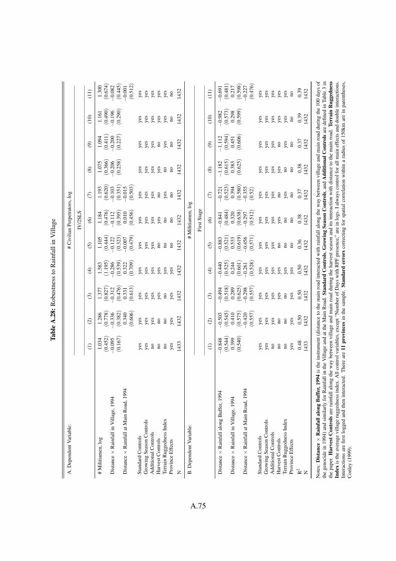
Tabl
eA
.28:
Rob
ustn
ess
toR
ainf
alli
nV
illag
e
A.D
epen
dent
Var
iabl
e:#
Civ
ilian
Perp
etra
tors
,log
IV/2
SLS
(1)
(2)
(3)
(4)
(5)
(6)
(7)
(8)
(9)
(10)
(11)
#M
ilitia
men
,log
1.03
41.
286
1.37
71.
583
1.10
51.
184
1.19
31.
075
1.09
41.
161
1.30
0(0
.452)
(0.7
78)
(0.8
27)
(1.1
95)
(0.4
44)
(0.4
76)
(0.6
20)
(0.3
66)
(0.4
11)
(0.4
90)
(0.6
74)
Dis
tanc
e×
Rai
nfal
lin
Vill
age,
1994
−0.
095
−0.
336
−0.
312
−0.
286
−0.
122
−0.
112
−0.
103
−0.
206
−0.
200
−0.
196
−0.
082
(0.1
67)
(0.3
82)
(0.4
76)
(0.5
39)
(0.3
23)
(0.3
95)
(0.3
51)
(0.2
58)
(0.2
27)
(0.2
90)
(0.4
45)
Dis
tanc
e×
Rai
nfal
latM
ain
Roa
d,19
940.
340
0.33
10.
322
−0.
007
0.01
0−
0.01
5−
0.00
1(0
.606)
(0.6
13)
(0.7
09)
(0.4
79)
(0.4
56)
(0.5
03)
(0.5
12)
Stan
dard
Con
trol
sye
sye
sye
sye
sye
sye
sye
sye
sye
sye
sye
sG
row
ing
Seas
onC
ontr
ols
yes
yes
yes
yes
yes
yes
yes
yes
yes
yes
yes
Add
ition
alC
ontr
ols
noye
sye
sye
sye
sye
sye
sye
sye
sye
sye
sH
arve
stC
ontr
ols
nono
yes
yes
noye
sno
yes
noye
sye
sTe
rrai
nR
ugge
dnes
sIn
dex
nono
noye
sno
noye
sno
yes
yes
yes
Prov
ince
Eff
ects
yes
yes
yes
yes
nono
nono
nono
no
N14
3314
3214
3214
3214
3214
3214
3214
3214
3214
3214
32
B.D
epen
dent
Var
iabl
e:#
Mili
tiam
en,l
og
Firs
tSta
ge
(1)
(2)
(3)
(4)
(5)
(6)
(7)
(8)
(9)
(10)
(11)
Dis
tanc
e×
Rai
nfal
lalo
ngB
uffe
r,19
94−
0.84
8−
0.50
3−
0.49
4−
0.44
0−
0.88
3−
0.84
1−
0.72
1−
1.18
2−
1.11
2−
0.98
2−
0.69
1(0
.544)
(0.5
45)
(0.5
18)
(0.5
25)
(0.5
21)
(0.4
84)
(0.5
23)
(0.6
15)
(0.5
94)
(0.5
73)
(0.4
81)
Dis
tanc
e×
Rai
nfal
lin
Vill
age,
1994
0.39
90.
410
0.28
90.
244
0.53
30.
320
0.39
40.
383
0.45
10.
298
0.21
7(0
.540)
(0.5
75)
(0.6
25)
(0.6
01)
(0.6
19)
(0.6
38)
(0.5
80)
(0.6
25)
(0.6
06)
(0.5
99)
(0.5
98)
Dis
tanc
e×
Rai
nfal
latM
ain
Roa
d,19
94−
0.42
0−
0.29
8−
0.26
1−
0.45
6−
0.29
7−
0.35
5−
0.22
7(0
.557)
(0.5
57)
(0.5
28)
(0.5
71)
(0.5
12)
(0.5
2)(0
.476)
Stan
dard
Con
trol
sye
sye
sye
sye
sye
sye
sye
sye
sye
sye
sye
sG
row
ing
Seas
onC
ontr
ols
yes
yes
yes
yes
yes
yes
yes
yes
yes
yes
yes
Add
ition
alC
ontr
ols
noye
sye
sye
sye
sye
sye
sye
sye
sye
sye
sH
arve
stC
ontr
ols
nono
yes
yes
noye
sno
yes
noye
sye
sTe
rrai
nR
ugge
dnes
sIn
dex
nono
noye
sno
noye
sno
yes
yes
yes
Prov
ince
Eff
ects
yes
yes
yes
yes
nono
nono
nono
no
R2
0.48
0.50
0.50
0.50
0.36
0.38
0.37
0.38
0.37
0.39
0.39
N14
3314
3214
3214
3214
3214
3214
3214
3214
3214
3214
32
Not
es:
Dis
tanc
e×
Rai
nfal
lalo
ngB
uffe
r,19
94is
the
inst
rum
ent(
dist
ance
toth
em
ain
road
inte
ract
edw
ithra
infa
llal
ong
the
way
betw
een
villa
gean
dm
ain
road
duri
ngth
e10
0da
ysof
the
geno
cide
in19
94)a
ndsi
mila
rly
forR
ainf
alli
nth
eV
illag
ean
dat
the
Mai
nR
oad.
Stan
dard
Con
trol
s,G
row
ing
Seas
onC
ontr
ols,
and
Add
ition
alC
ontr
ols
are
defin
edin
Tabl
e3
inth
epa
per.
Har
vest
Con
trol
sar
era
infa
llal
ong
the
way
betw
een
villa
gean
dm
ain
road
duri
ngth
eha
rves
tsea
son
and
itsin
tera
ctio
nw
ithdi
stan
ceto
the
mai
nro
ad.
Terr
ain
Rug
gedn
ess
Inde
xis
the
aver
age
villa
geru
gged
ness
inde
x.A
llco
ntro
lvar
iabl
es,e
xcep
t“N
umbe
rofD
ays
with
RPF
pres
ence
,”ar
ein
logs
.Ial
way
sco
ntro
lfor
allm
ain
effe
cts
and
doub
lein
tera
ctio
ns.
Inte
ract
ions
are
first
logg
edan
dth
enin
tera
cted
.T
here
are
11pr
ovin
ces
inth
esa
mpl
e.St
anda
rder
rors
corr
ectin
gfo
rsp
atia
lcor
rela
tion
with
ina
radi
usof
150k
mar
ein
pare
nthe
ses,
Con
ley
(199
9).
A.75

A.5 Extensions to Section V. – Network Effects
A.5.1 A Simple Spatial Model
To guide the empirical analysis in the paper, I use a simple game-theoretic modelto determine the allocation of militiamen and their effects on civilian participa-tion. The model is based on Acemoglu, Garcia-Jimeno and Robinson (2015).
A.5.2 Network Structure and Utility
Assume that the economy consists of n villages. For village i let N(i) denotethe set of villages that are connected to it. In the baseline these will be the directneighbors to i but I will also present results when using higher-order neighbors.Let W be an n×n symmetric, spatial weighting matrix with off-diagonal entriesgiven by
(A.1) wi j =
0 if j /∈ N(i)1
di jri jif j ∈ N(i),
where di j denotes the geodesic distance between the centroids of villages i andj and ri j is the amount of rainfall along the way between villages i and j. Thuspossible spillovers between villages depend on the transport costs between thevillages. In particular, heavy rainfall makes transportation and thus spilloversharder.
Civilian participation in violence is a function of the number of militiamenin each village and the number of militiamen in neighboring villages
(A.2) ci = τimi + ηtimi + φmiWim+ δWim+ ui,
where ci is the number of civilian perpetrators in village i and mi are the numberof militiamen in village i. Wi is the ith row of the spatial weighting matrix Wand m is the full column vector of militiamen, respectively. Besides, the effectof village i’s militia on civilian violence depends on village characteristics inthe following way
(A.3) τi = Xiβ + γpi + εi,
A.76
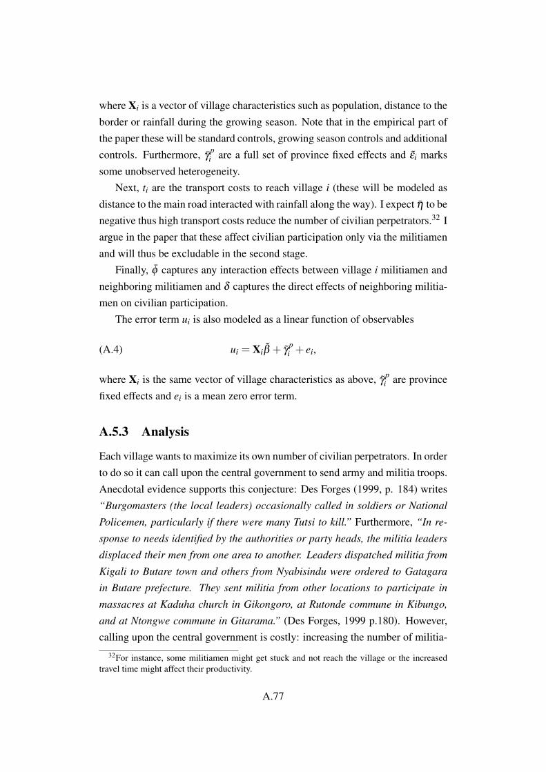
where Xi is a vector of village characteristics such as population, distance to theborder or rainfall during the growing season. Note that in the empirical part ofthe paper these will be standard controls, growing season controls and additionalcontrols. Furthermore, γ
pi are a full set of province fixed effects and εi marks
some unobserved heterogeneity.Next, ti are the transport costs to reach village i (these will be modeled as
distance to the main road interacted with rainfall along the way). I expect η to benegative thus high transport costs reduce the number of civilian perpetrators.32 Iargue in the paper that these affect civilian participation only via the militiamenand will thus be excludable in the second stage.
Finally, φ captures any interaction effects between village i militiamen andneighboring militiamen and δ captures the direct effects of neighboring militia-men on civilian participation.
The error term ui is also modeled as a linear function of observables
(A.4) ui = Xiβ + γpi + ei,
where Xi is the same vector of village characteristics as above, γpi are province
fixed effects and ei is a mean zero error term.
A.5.3 Analysis
Each village wants to maximize its own number of civilian perpetrators. In orderto do so it can call upon the central government to send army and militia troops.Anecdotal evidence supports this conjecture: Des Forges (1999, p. 184) writes“Burgomasters (the local leaders) occasionally called in soldiers or National
Policemen, particularly if there were many Tutsi to kill.” Furthermore, “In re-
sponse to needs identified by the authorities or party heads, the militia leaders
displaced their men from one area to another. Leaders dispatched militia from
Kigali to Butare town and others from Nyabisindu were ordered to Gatagara
in Butare prefecture. They sent militia from other locations to participate in
massacres at Kaduha church in Gikongoro, at Rutonde commune in Kibungo,
and at Ntongwe commune in Gitarama.” (Des Forges, 1999 p.180). However,calling upon the central government is costly: increasing the number of militia-
32For instance, some militiamen might get stuck and not reach the village or the increasedtravel time might affect their productivity.
A.77
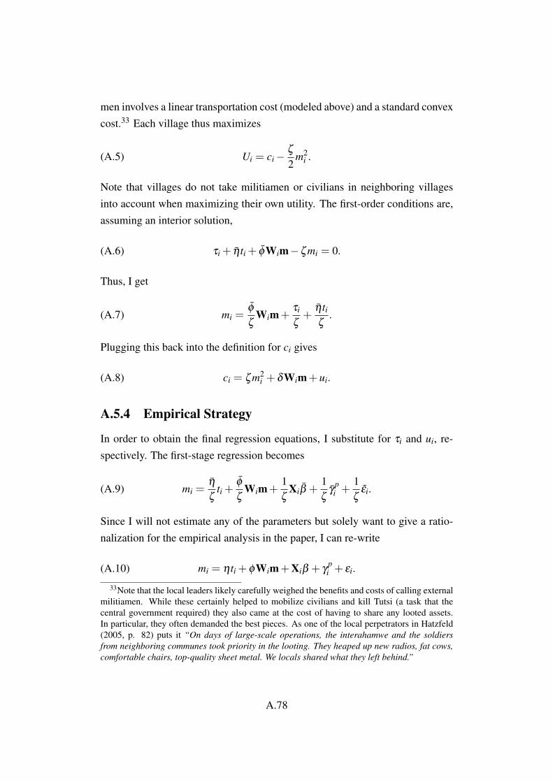
men involves a linear transportation cost (modeled above) and a standard convexcost.33 Each village thus maximizes
(A.5) Ui = ci−ζ
2m2
i .
Note that villages do not take militiamen or civilians in neighboring villagesinto account when maximizing their own utility. The first-order conditions are,assuming an interior solution,
(A.6) τi + ηti + φWim−ζ mi = 0.
Thus, I get
(A.7) mi =φ
ζWim+
τi
ζ+
ηtiζ
.
Plugging this back into the definition for ci gives
(A.8) ci = ζ m2i + δWim+ ui.
A.5.4 Empirical Strategy
In order to obtain the final regression equations, I substitute for τi and ui, re-spectively. The first-stage regression becomes
(A.9) mi =η
ζti +
φ
ζWim+
1ζ
Xiβ +1ζ
γpi +
1ζ
εi.
Since I will not estimate any of the parameters but solely want to give a ratio-nalization for the empirical analysis in the paper, I can re-write
(A.10) mi = ηti +φWim+Xiβ + γpi + εi.
33Note that the local leaders likely carefully weighed the benefits and costs of calling externalmilitiamen. While these certainly helped to mobilize civilians and kill Tutsi (a task that thecentral government required) they also came at the cost of having to share any looted assets.In particular, they often demanded the best pieces. As one of the local perpetrators in Hatzfeld(2005, p. 82) puts it “On days of large-scale operations, the interahamwe and the soldiersfrom neighboring communes took priority in the looting. They heaped up new radios, fat cows,comfortable chairs, top-quality sheet metal. We locals shared what they left behind.”
A.78

In this first stage ti is the militia’s transport costs measured as the distance ofthe village centroid from the main road interacted with rainfall along the wayfrom the village to the main road during the time of the genocide. Note that thetwo main effects, i.e. distance and rainfall uninteracted, are included in Xi. Thenew term Wim captures any spillover or displacement effects. Depending onthe sign of φ militiamen arriving in neighboring villages can either increase thenumber of militiamen in village i (φ positive) if militiamen for instance move toneighboring villages once their mission is completed or decrease the number ofmilitiamen if there are displacement effects (φ negative).
The second-stage regression becomes
(A.11) ci = ζ m2i + δWim+Xiβ + γ
pi + ei.
Here the new terms Wim capture possible spillover effects. In particular, anyspillover effects in equation (A.10) are likely to be mirrored in the second stage(A.11), captured by δ .
Finally note that strictly speaking this model predicts a quadratic relation-ship between ci and mi. In the empirical analysis in the paper I deviate from thisas I anyway take the natural logarithm of the two conflict variables.
A.5.5 Identification
Note that because of the recursive structure of the specification Wim is likely tobe correlated with the error term and thus endogenous in the first stage. Besides,both mi and neighboring militiamen Wim are endogenous in the second stage.To obtain causal effects I follow the standard procedure in the spatial econo-metrics literature and use instruments constructed using the characteristics ofneighbors’ of neighbors.
The idea is that transport costs (and other characteristics) to second-orderneighbors affect the number of militiamen in a given village i only via the num-ber of militiamen going to first-order neighbors. Note that the point estimateson the spillover terms obtained for regressions (A.10) and (A.11), although in-formative about the direction of potential spillover effects, do not allow me todirectly read off marginal effects. I will use the standard formulas to calculate
A.79
direct, indirect and total marginal effects.34
A.5.6 Additional Tables
34In general, one can re-write the specifications above as y=Xβ +WXπ+λWy+e. Solvingthis equation for y yields: y = (I−λW)−1(Xβ +WXπ + e). Furthermore, E(y|X,W) = (I−λW)−1[Xβ +WXπ ]. The marginal direct effect is ADE = 1
n ∑ni=1
∂E(yi|X,W)∂xi
and the indirect
effect is given by AIE = 1n ∑
ni=1 ∑
nj=1, j 6=i
∂E(yi|X,W)∂xi
. The total effect is the sum of the two.
A.80

Tabl
eA
.29:
Spat
ialE
cono
my
ofC
onfli
ct–
Hig
her-
Ord
erN
eigh
bors
Rob
ustn
ess
Dep
ende
ntV
aria
ble:
#M
ilitia
men
,log
Spat
ialL
ag:
X=
3X=
4X=
5X=
6
(1)
(2)
(3)
(4)
(5)
(6)
(7)
(8)
Dis
tanc
e×
Rai
nfal
lalo
ngB
uffe
r,19
94−
0.51
6−
0.51
0−
0.49
9−
0.52
2−
0.49
3−
0.51
5−
0.49
1−
0.50
4(0
.133)
(0.1
36)
(0.1
31)
(0.1
32)
(0.1
31)
(0.1
32)
(0.1
30)
(0.1
30)
Spat
ialL
agof
Ord
erX×
#M
ilitia
men
,log
0.02
70.
022
−0.
035
−0.
015
−0.
057
−0.
026
−0.
065
−0.
050
(0.0
67)
(0.0
67)
(0.0
62)
(0.0
56)
(0.0
59)
(0.0
49)
(0.0
57)
(0.1
16)
Stan
dard
Con
trol
sye
sye
sye
sye
sye
sye
sye
sye
sG
row
ing
Seas
onC
ontr
ols
yes
yes
yes
yes
yes
yes
yes
yes
Add
ition
alC
ontr
ols
yes
yes
yes
yes
yes
yes
yes
yes
Prov
ince
Eff
ects
yes
yes
yes
yes
yes
yes
yes
yes
Mar
gina
lEff
ects
ofth
eIn
stru
men
tD
irec
tEff
ect
−0.
516
−0.
510
−0.
499
−0.
522
−0.
493
−0.
515
−0.
491
−0.
504
(0.1
33)
(0.1
36)
(0.1
31)
(0.1
32)
(0.1
31)
(0.1
32)
(0.1
30)
(0.1
30)
Indi
rect
Eff
ect
−0.
002
−0.
002
0.00
20.
001
0.00
20.
001
0.00
20.
001
(0.0
05)
(0.0
05)
(0.0
03)
(0.0
03)
(0.0
02)
(0.0
02)
(0.0
02)
(0.0
03)
Tota
lEff
ect
−0.
518
−0.
512
−0.
497
−0.
521
−0.
491
−0.
514
−0.
489
−0.
503
(0.1
35)
(0.1
38)
(0.1
32)
(0.1
32)
(0.1
31)
(0.1
32)
(0.1
30)
(0.1
31)
N14
3214
3214
3214
3214
3214
3214
3214
32
Not
es:
Spat
ialL
agof
Ord
erX×
#M
ilitia
men
,log
isth
enu
mbe
rofm
ilitia
men
mul
tiplie
dby
anX
th-O
rder
spat
ialw
eigh
ting
mat
rix.
The
wei
ghts
forn
eigh
bors
are
defin
edas
1di
stij×
rain
ij,t
heX
’sar
ede
fined
inth
eco
lum
nhe
ader
s.St
anda
rdC
ontr
ols,
Gro
win
gSe
ason
Con
trol
s,an
dA
dditi
onal
Con
trol
sare
defin
edin
Tabl
e3
inth
epa
per.
Inte
ract
ions
are
first
logg
edan
dth
enin
tera
cted
.T
here
are
11pr
ovin
ces
inth
esa
mpl
e.In
allo
ddre
gres
sion
ssp
atia
laut
o-co
rrel
atio
nsp
atia
laut
o-co
rrel
atio
nis
assu
med
tobe
capt
ured
byth
esp
atia
llag
ofth
ede
pend
entv
aria
ble
and
erro
rter
ms
are
hete
rosk
edas
tic(C
onle
y,20
08).
Inal
leve
nre
gres
sion
ssp
atia
laut
o-co
rrel
atio
nis
expl
icitl
ym
odel
edin
the
erro
rter
mfo
llow
ing
Dru
kker
etal
.(20
13).
Stan
dard
erro
rsfo
rmar
gina
leff
ects
are
obta
ined
usin
gth
ede
ltam
etho
d.
A.81

Tabl
eA
.30:
Spat
ialE
cono
my
ofC
onfli
ct–
Spat
ialW
eigh
tsR
obus
tnes
s
Dep
ende
ntV
aria
ble:
#C
ivili
an#
Mili
tiam
en,l
ogPe
rpet
rato
rs,l
og
Spat
ialL
ag:
X=
1X=
2X=
3X=
4X=
5X=
6X=
1
(1)
(2)
(3)
(4)
(5)
(6)
(7)
(8)
(9)
(10)
(11)
(12)
(13)
Dis
tanc
e×
Rai
nfal
lalo
ngB
uffe
r,19
94−
0.49
8−
0.49
7−
0.56
4−
0.52
2−
0.56
7−
0.48
0−
0.55
7−
0.53
6−
0.54
0−
0.53
3−
0.52
7−
0.54
9(0
.132)
(0.1
38)
(0.1
34)
(0.1
48)
(0.1
34)
(0.1
52)
(0.1
34)
(0.1
45)
(0.1
34)
(0.1
39)
(0.1
34)
(0.1
34)
#M
ilitia
men
,log
1.29
1(0
.074)
Spat
ialL
agof
Ord
erX×
#M
ilitia
men
,log
0.45
10.
446
0.35
70.
409
0.24
70.
534
0.15
30.
133
0.09
00.
073
0.04
80.
038
0.01
6(0
.062)
(0.0
62)
(0.0
62)
(0.0
73)
(0.0
60)
(0.1
14)
(0.0
58)
(0.0
67)
(0.0
56)
(0.0
62)
(0.0
54)
(0.0
54)
(0.0
30)
Stan
dard
Con
trol
sye
sye
sye
sye
sye
sye
sye
sye
sye
sye
sye
sye
sye
sG
row
ing
Seas
onC
ontr
ols
yes
yes
yes
yes
yes
yes
yes
yes
yes
yes
yes
yes
yes
Add
ition
alC
ontr
ols
yes
yes
yes
yes
yes
yes
yes
yes
yes
yes
yes
yes
yes
Prov
ince
Eff
ects
yes
yes
yes
yes
yes
yes
yes
yes
yes
yes
yes
yes
yes
Mar
gina
lEff
ects
Dir
ectE
ffec
t−
0.50
8−
0.50
7−
0.56
6−
0.52
4−
0.56
8−
0.48
2−
0.55
7−
0.53
6−
0.54
0−
0.53
3−
0.52
7−
0.54
91.
292
(0.1
35)
(0.1
41)
(0.1
34)
(0.1
48)
(0.1
34)
(0.1
53)
(0.1
34)
(0.1
45)
(0.1
34)
(0.1
39)
(0.1
34)
(0.1
34)
(0.0
74)
Indi
rect
Eff
ect
−0.
196
−0.
192
−0.
116
−0.
128
−0.
053
−0.
121
−0.
024
−0.
020
−0.
010
−0.
008
−0.
004
−0.
004
0.01
0(0
.067)
(0.0
67)
(0.0
41)
(0.0
50)
(0.0
22)
(0.0
54)
(0.0
13)
(0.0
13)
(0.0
08)
(0.0
08)
(0.0
06)
(0.0
05)
(0.0
19)
Tota
lEff
ect
−0.
703
−0.
698
−0.
681
−0.
652
−0.
621
−0.
603
−0.
581
−0.
556
−0.
550
−0.
542
−0.
531
−0.
553
1.30
2(0
.194)
(0.2
01)
(0.1
68)
(0.1
91)
(0.1
51)
(0.1
95)
(0.1
43)
(0.1
52)
(0.1
38)
(0.1
43)
(0.1
36)
(0.1
36)
(0.0
72)
N14
3214
3214
3214
3214
3214
3214
3214
3214
3214
3214
3214
3214
32
Not
es:
Spat
ialL
agof
Ord
erX×
#M
ilitia
men
,log
isth
enu
mbe
rof
mili
tiam
enm
ultip
lied
byan
Xth
-Ord
ersp
atia
lwei
ghtin
gm
atri
x.T
hew
eigh
tsfo
rne
ighb
ors
are
defin
edas
1di
stij
,the
X’s
are
defin
edin
the
colu
mn
head
ers.
Stan
dard
Con
trol
s,G
row
ing
Seas
onC
ontr
ols,
and
Add
ition
alC
ontr
olsa
rede
fined
inTa
ble
3in
the
pape
r.In
tera
ctio
nsar
efir
stlo
gged
and
then
inte
ract
ed.T
here
are
11pr
ovin
cesi
nth
esa
mpl
e.In
alle
ven
regr
essi
ons
spat
iala
uto-
corr
elat
ion
isex
plic
itly
mod
eled
inth
eer
rort
erm
follo
win
gD
rukk
eret
al.
(201
3).
Inre
gres
sion
13st
anda
rder
rors
are
corr
ecte
dfo
rspa
tialc
orre
latio
nw
ithin
ara
dius
of15
0km
,C
onle
y(1
999)
.In
allo
ther
regr
essi
ons
spat
iala
uto-
corr
elat
ion
isas
sum
edto
beca
ptur
edby
the
spat
iall
agof
the
depe
nden
tvar
iabl
ean
der
rort
erm
sar
ehe
tero
sked
astic
(Con
ley,
2008
).
A.82

A.6 Extensions to Section VI. – The Tutsi Minor-ity, Material Incentives, Fear, and RTLM
The results from Section VI. in the paper suggest that the militia mostly actedas a moral authority invoking civilians’ obedience. In this Section I considersome additional interaction effects to understand the channels better. Note that,in order to establish causality, I instrument each interaction term with the in-teraction between the instrument and the variable capturing the heterogeneouseffects. Furthermore, I always include all double interactions.
Tutsi Minority First, the militia’s effects on civilian participation are larger invillages with Tutsi rebels present at the beginning of the genocide (regressions1 and 2 in Table A.31). Since the Hutu extremists carefully cultivated the Hutupopulations fear of the Tutsi (rebels), mobilizing the population in these villageswas likely easier. Additionally, villages with Tutsi rebels had much fewer localmilitiamen and thus the arriving external militiamen likely had a large impact.35
Second, the coefficient on the interaction with the Tutsi minority share, isequally positive (5.161, standard error 13.810, regression 1). However, sincevariation in the Tutsi minority share only comes at coarse commune level, theeffect is insignificant. In regression 2, I thus replace the continuous Tutsi mi-nority share variable by a dummy variable taking on the value of 1 if the Tutsiminority share lies above the median. Once more, the point estimate is similarlypositive but, in addition, also significant at the 95 percent level (1.070, standarderror 0.531).36
A large Tutsi minority likely made mobilization easier as the enemy waseasy to point out. In addition, similar to the case for Tutsi rebels, villageswith large Tutsi minorities likely had fewer local militiamen, thus increasingthe marginal effect of an external militia member.
35Note that this explanation assumes that the effects of the militia on civilian participationare concave and that local and external militiamen are substitutes in the mobilization process. Iprovide evidence for this below.
36Unfortunately, because of strong multicollinearity, this specification does not allow me tocontrol for the double interaction of the Tutsi minority share dummy with distance to the mainroad. To account for the potential omitted variable bias that this creates, I interact the Tutsi mi-nority share dummy with the other controls not involving distance to the main road and includethem in the regression.
A.83

Material Incentives There is abundant anecdotal evidence that material in-centives mattered for civilian participation (Hatzfeld, 2005). In regressions 3 to5, I test this. Importantly, I differentiate between Hutu wealth and Tutsi wealth.Theory suggests two opposite effects of income on conflict (Dube and Vargas,2013). Conflict levels should increase if the gains from fighting go up, this isthe rapacity channel. On the other hand, conflict prevalence should decreaseif income from alternative economic activities goes up, this is the opportunitycost channel. Thus, in this case, since the Hutu attacked the Tutsi, an increasein Tutsi wealth should make mobilization easier and an increase in Hutu wealthshould decrease participation. Regressions 3 to 5 confirm these conjectures.The interaction effect with Hutu wealth is negative and statistically significantat the 95 percent level (-0.620, standard error 0.248). For Tutsi wealth the in-teraction is positive and again statistically significant (regression 4). The resultsare robust to adding both interactions together (regression 5).
Note that these results are consistent with the result from the main paper thatthe militia did not coerce civilians but rather invoked obedience. If the militiahad coerced civilians this should have happened regardless of the material statusof the village. However, acting as a moral authority suggests that there was someroom for discretion.
Reassuringly, the above results are robust to including both wealth and Tutsiinteractions (regression 6).
Prior Exposure to Violence Finally, I check whether a village’s prior expo-sure to violence affects the results. The Uppsala Conflict Data Program (UCDP)database (Pettersson and Oberg, 2020; UCDP, 2013; Sundberg and Melander,2013) provides detailed information on the location and actors of violent eventssince 1989.37 Results are reported in Table A.32. First, I show that my instru-ment is uncorrelated with whether a village experienced pre-genocide violence(regression 1). Second, the militia’s effects on civilian participation seem to belower in places with prior violence (regression 2). The point estimate on theinteraction term is negative, however strongly insignificant. Because exposureto Hutu-driven and RPF-driven violence may have had different effects, I nextsplit villages into those who experienced any kind of RPF violence and those
37The main sources of UCDP are reports by international news agencies (such as Reuters andthe BBC) and reports from non-governmental organizations (such as Human Rights Watch).
A.84

that only experienced Hutu violence (against Tutsi civilians). The effects inregression 3 suggest that the militia was especially successful in villages withexposure to RPF violence. The point estimate is positive and significant at the 90percent level (2.853, standard error 1.570). The point estimate on Hutu violenceis negative but still highly insignificant. These results are robust to interact-ing the two violence measures in two separate regressions (regressions 4 and5). In this case, significance for the RPF violence interaction increases slightly(regression 4).
In terms of interpretation, these results are consistent with anecdotal evi-dence suggesting that the Hutu government built on the population’s fear of theTutsi and especially the Tutsi rebel army to foster participation (Des Forges,1999). This fear should have been especially salient in those places that wereexposed to pre-genocide Tutsi violence. Once more the findings are inconsis-tent with the militia coercing civilians into participation. In that case, the effectsshould have been unrelated to RPF violence exposure.
RTLM As an extension, I look at interaction effects with RTLM coverage inTable A.33. Recall from the main paper that RTLM induced violence by localmilitia and police forces (and only subsequently civilians). Thus this delivers atest on whether external and local militia were substitutes or complemented eachother. I first interact the number of militiamen with a dummy taking on the valueof 1 if RTLM coverage lies above the median. The effect is close to zero andinsignificant. This is confirmed when I, instead of interacting, split the sampleat the median of RTLM (regressions 3 and 4). Both effects are significant andhighly similar. Note that the effects are slightly lower than my baseline resultsfrom the main paper. This is because the RTLM sample is slightly smaller: inregression 7 I rerun my baseline specification using the RTLM sample and thepoint estimate is similar to the ones in regressions 3 and 4.
Finally, I split the sample at the 75th percentile. The interaction effect inregression 2 suggests that the effects of the militia are lower in places with highRTLM coverage (above 75th percentile). The effect is almost significant at the90 percent level (when using clustered standard errors). Note that because ofthe stark differences between clustered and Conley standard errors in this case,I report both. This negative interaction effect is confirmed when splitting thesample at the 75th percentile. While the effect for villages with low RTLM
A.85
coverage is close to baseline and highly significant, the effect for high-RTLMvillages is low and insignificant (0.243, standard errors 0.366 and 0.289). Thissuggests that local and external militiamen were substitutes in the mobilizationprocess.
References
[1] Des Forges, A. 1999. Leave None to Tell the Story: Genocide in Rwanda,New York: Human Rights Watch.
[2] Dube, O. and J. F. Vargas. 2013. Commodity Price Shocks and Civil Con-flict: Evidence From Colombia, Review of Economic Studies, 80(4): 1384-1421.
[3] Hatzfeld, J. 2005. Machete season: The Killers in Rwanda speak, NewYork: Picador.
[4] Pettersson, T. and M. Oberg. 2020. Organized Violence, 1989-2019. Jour-
nal of Peace Research, 57(4): 597-613.
[5] Sundberg, R. and E. Melander. 2013. Introducing the UCDP Geo-Referenced Event Dataset. Journal of Peace Research, 50(4): 523-532.
[6] Uppsala Conflict Data Program (UCDP). 2013. UCDP Geo-ReferencedEvent Dataset. https://ucdp.uu.se/downloads/index.htmlged global (ac-cessed July 2020).
A.86
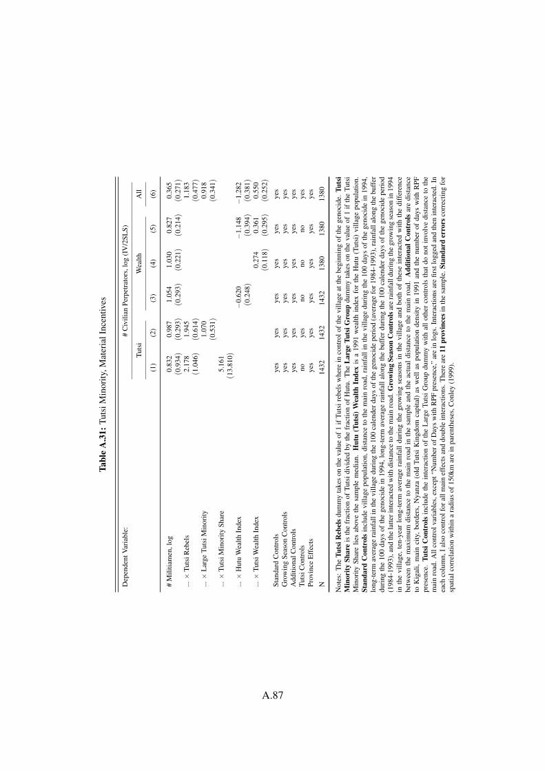
Tabl
eA
.31:
Tuts
iMin
ority
,Mat
eria
lInc
entiv
es
Dep
ende
ntV
aria
ble:
#C
ivili
anPe
rpet
rato
rs,l
og(I
V/2
SLS)
Tuts
iW
ealth
All
(1)
(2)
(3)
(4)
(5)
(6)
#M
ilitia
men
,log
0.83
20.
987
1.05
41.
030
0.82
70.
365
(0.9
34)
(0.2
93)
(0.2
93)
(0.2
21)
(0.2
14)
(0.2
71)
...×
Tuts
iReb
els
2.17
81.
945
1.18
3(1
.046)
(0.6
14)
(0.4
77)
...×
Lar
geTu
tsiM
inor
ity1.
070
0.91
8(0
.531)
(0.3
41)
...×
Tuts
iMin
ority
Shar
e5.
161
(13.
810)
...×
Hut
uW
ealth
Inde
x−
0.62
0−
1.14
8−
1.28
2(0
.248)
(0.3
94)
(0.3
81)
...×
Tuts
iWea
lthIn
dex
0.27
40.
361
0.55
0(0
.118)
(0.2
95)
(0.2
52)
Stan
dard
Con
trol
sye
sye
sye
sye
sye
sye
sG
row
ing
Seas
onC
ontr
ols
yes
yes
yes
yes
yes
yes
Add
ition
alC
ontr
ols
yes
yes
yes
yes
yes
yes
Tuts
iCon
trol
sno
yes
nono
noye
sPr
ovin
ceE
ffec
tsye
sye
sye
sye
sye
sye
s
N14
3214
3214
3213
8013
8013
80
Not
es:
The
Tuts
iReb
els
dum
my
take
son
the
valu
eof
1if
Tuts
ireb
els
whe
rein
cont
rolo
fthe
villa
geat
the
begi
nnin
gof
the
geno
cide
.Tu
tsi
Min
ority
Shar
eis
the
frac
tion
ofTu
tsid
ivid
edby
the
frac
tion
ofH
utu.
The
Lar
geTu
tsiG
roup
dum
my
take
son
the
valu
eof
1if
the
Tuts
iM
inor
itySh
are
lies
abov
eth
esa
mpl
em
edia
n.H
utu
(Tut
si)
Wea
lthIn
dex
isa
1991
wea
lthin
dex
for
the
Hut
u(T
utsi
)vi
llage
popu
latio
n.St
anda
rdC
ontr
ols
incl
ude
villa
gepo
pula
tion,
dist
ance
toth
em
ain
road
,rai
nfal
lin
the
villa
gedu
ring
the
100
days
ofth
ege
noci
dein
1994
,lo
ng-t
erm
aver
age
rain
fall
inth
evi
llage
duri
ngth
e10
0ca
lend
erda
ysof
the
geno
cide
peri
od(a
vera
gefo
r198
4-19
93),
rain
fall
alon
gth
ebu
ffer
duri
ngth
e10
0da
ysof
the
geno
cide
in19
94,l
ong-
term
aver
age
rain
fall
alon
gth
ebu
ffer
duri
ngth
e10
0ca
lend
erda
ysof
the
geno
cide
peri
od(1
984-
1993
),an
dth
ela
tteri
nter
acte
dw
ithdi
stan
ceto
the
mai
nro
ad.G
row
ing
Seas
onC
ontr
olsa
rera
infa
lldu
ring
the
grow
ing
seas
onin
1994
inth
evi
llage
,ten
-yea
rlo
ng-t
erm
aver
age
rain
fall
duri
ngth
egr
owin
gse
ason
sin
the
villa
gean
dbo
thof
thes
ein
tera
cted
with
the
diff
eren
cebe
twee
nth
em
axim
umdi
stan
ceto
the
mai
nro
adin
the
sam
ple
and
the
actu
aldi
stan
ceto
the
mai
nro
ad.
Add
ition
alC
ontr
ols
are
dist
ance
toK
igal
i,m
ain
city
,bo
rder
s,N
yanz
a(o
ldTu
tsi
Kin
gdom
capi
tal)
asw
ell
aspo
pula
tion
dens
ityin
1991
and
the
num
ber
ofda
ysw
ithR
PFpr
esen
ce.
Tuts
iCon
trol
sin
clud
eth
ein
tera
ctio
nof
the
Lar
geTu
tsiG
roup
dum
my
with
allo
ther
cont
rols
that
dono
tinv
olve
dist
ance
toth
em
ain
road
.All
cont
rolv
aria
bles
,exc
ept“
Num
bero
fDay
sw
ithR
PFpr
esen
ce,”
are
inlo
gs.I
nter
actio
nsar
efir
stlo
gged
and
then
inte
ract
ed.I
nea
chco
lum
n,Ia
lso
cont
rolf
oral
lmai
nef
fect
san
ddo
uble
inte
ract
ions
.The
rear
e11
prov
ince
sin
the
sam
ple.
Stan
dard
erro
rsco
rrec
ting
for
spat
ialc
orre
latio
nw
ithin
ara
dius
of15
0km
are
inpa
rent
hese
s,C
onle
y(1
999)
.
A.87
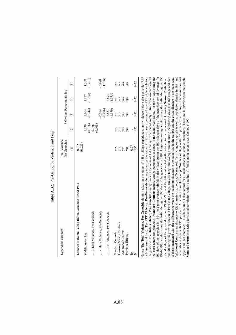
Tabl
eA
.32:
Pre-
Gen
ocid
eV
iole
nce
and
Fear
Dep
ende
ntV
aria
ble:
Tota
lVio
lenc
ePr
e-G
enoc
ide
#C
ivili
anPe
rpet
rato
rs,l
og
(1)
(2)
(3)
(4)
(5)
Dis
tanc
e×
Rai
nfal
lalo
ngB
uffe
r,G
enoc
ide
Peri
od19
94−
0.01
5(0
.023)
#M
ilitia
men
,log
1.33
01.
104
1.13
71.
308
(0.3
16)
(0.2
44)
(0.2
24)
(0.4
51)
...×
Tota
lVio
lenc
e,Pr
e-G
enoc
ide
−0.
926
(0.6
68)
...×
Hut
uV
iole
nce,
Pre-
Gen
ocid
e−
0.69
4−
0.98
0(0
.496)
(1.7
36)
...×
RPF
Vio
lenc
e,Pr
e-G
enoc
ide
2.85
32.
694
(1.5
70)
(1.5
35)
Stan
dard
Con
trol
sye
sye
sye
sye
sye
sG
row
ing
Seas
onC
ontr
ols
yes
yes
yes
yes
yes
Add
ition
alC
ontr
ols
yes
yes
yes
yes
yes
Prov
ince
Eff
ects
yes
yes
yes
yes
yes
R2
0.27
..
..
N14
3214
3214
3214
3214
32
Not
es:
The
Tota
lVio
lenc
e,Pr
e-G
enoc
ide
dum
my
take
son
the
valu
eof
1if
avi
llage
expe
rien
ced
any
viol
ence
befo
reth
ege
noci
de(R
PFor
Hut
uar
my
driv
en).
The
RPF
Vio
lenc
e,Pr
e-G
enoc
ide
dum
my
take
son
the
valu
eof
1if
avi
llage
expe
rien
ced
any
RPF
viol
ence
befo
reth
ege
noci
de.
The
Hut
uV
iole
nce,
Pre-
Gen
ocid
edu
mm
yta
kes
onth
eva
lue
of1
ifa
villa
geex
peri
ence
dso
lely
Hut
u-dr
iven
viol
ence
agai
nst
the
Tuts
ibe
fore
the
geno
cide
.St
anda
rdC
ontr
ols
incl
ude
villa
gepo
pula
tion,
dist
ance
toth
em
ain
road
,ra
infa
llin
the
villa
gedu
ring
the
100
days
ofth
ege
noci
dein
1994
,lon
g-te
rmav
erag
era
infa
llin
the
villa
gedu
ring
the
100
cale
nder
days
ofth
ege
noci
depe
riod
(ave
rage
for
1984
-199
3),r
ainf
alla
long
the
buff
erdu
ring
the
100
days
ofth
ege
noci
dein
1994
,lon
g-te
rmav
erag
era
infa
llal
ong
the
buff
erdu
ring
the
100
cale
nder
days
ofth
ege
noci
depe
riod
(198
4-19
93),
and
the
latte
rin
tera
cted
with
dist
ance
toth
em
ain
road
.G
row
ing
Seas
onC
ontr
ols
are
rain
fall
duri
ngth
egr
owin
gse
ason
in19
94in
the
villa
ge,t
en-y
earl
ong-
term
aver
age
rain
fall
duri
ngth
egr
owin
gse
ason
sin
the
villa
gean
dbo
thof
thes
ein
tera
cted
with
the
diff
eren
cebe
twee
nth
em
axim
umdi
stan
ceto
the
mai
nro
adin
the
sam
ple
and
the
actu
aldi
stan
ceto
the
mai
nro
ad.
Add
ition
alC
ontr
olsa
redi
stan
ceto
Kig
ali,
mai
nci
ty,b
orde
rs,N
yanz
a(o
ldTu
tsiK
ingd
omca
pita
l)as
wel
las
popu
latio
nde
nsity
in19
91an
dth
enu
mbe
rof
days
with
RPF
pres
ence
.A
llco
ntro
lvar
iabl
es,e
xcep
t“N
umbe
rof
Day
sw
ithR
PFpr
esen
ce,”
are
inlo
gs.
Inte
ract
ions
are
first
logg
edan
dth
enin
tera
cted
.In
each
colu
mn,
Ial
soco
ntro
lfor
allm
ain
effe
cts
and
doub
lein
tera
ctio
ns.
The
rear
e11
prov
ince
sin
the
sam
ple.
Stan
dard
erro
rsco
rrec
ting
fors
patia
lcor
rela
tion
with
ina
radi
usof
150k
mar
ein
pare
nthe
ses,
Con
ley
(199
9).
A.88

Tabl
eA
.33:
RT
LM
Inte
ract
ion
Eff
ects #
Civ
ilian
Perp
etra
tors
,log
Full
Rad
ioC
over
age
Rad
ioC
over
age
Rad
ioC
over
age
Rad
ioC
over
age
Full
Sam
ple
abov
eM
edia
nbe
low
Med
ian
abov
e75
thbe
low
75th
Sam
ple
(1)
(2)
(3)
(4)
(5)
(6)
(7)
#M
ilitia
men
,log
1.03
71.
406
1.06
40.
925
0.24
31.
293
1.00
7(0
.741)
(0.6
82)
(0.4
29)
(0.4
60)
(0.3
66)
(0.4
55)
(0.3
03)
[16.
550]
[22.
720]
[0.2
62]
[0.3
92]
[0.2
89]
[0.4
49]
[0.2
46]
...x
RT
LM
Rad
ioC
over
age,
dum
my
(med
ian)
0.02
1(0
.790)
[8.4
19]
...x
RT
LM
Rad
ioC
over
age,
dum
my
(75t
h)−
0.72
8(0
.469)
[11.
390]
Stan
dard
Con
trol
sye
sye
sye
sye
sye
sye
sye
sG
row
ing
Seas
onC
ontr
ols
yes
yes
yes
yes
yes
yes
yes
Add
ition
alC
ontr
ols
yes
yes
yes
yes
yes
yes
yes
Prop
agat
ion
Con
trol
sye
sye
sno
nono
nono
Add
ition
alR
adio
Con
trol
sye
sye
sno
nono
nono
Prov
ince
Eff
ects
yes
yes
yes
yes
yes
yes
yes
N10
5610
5652
952
726
479
210
56
Not
es:
Reg
ress
ions
1,2
and
7us
eth
efu
llR
TL
Msa
mpl
em
atch
edw
ithm
ysa
mpl
e.In
regr
essi
ons
3an
d4
the
sam
ple
issp
litat
the
med
ian
valu
eof
RT
LM
cove
rage
.In
regr
essi
ons5
and
6th
esa
mpl
eis
split
atth
e75
thpe
rcen
tile
ofR
TL
Mco
vera
ge.S
tand
ard
Con
trol
s,G
row
ing
Seas
onC
ontr
ols,
and
Add
ition
alC
ontr
olsa
rede
fined
inTa
ble
3in
the
pape
r.Pr
opag
atio
nco
ntro
lsar
e:la
titud
e,lo
ngitu
de,a
seco
ndor
der
poly
nom
iali
nvi
llage
mea
nal
titud
e,vi
llage
altit
ude
vari
ance
,and
ase
cond
orde
rpo
lyno
mia
lin
the
dist
ance
toth
ene
ares
ttra
nsm
itter
.Add
ition
alR
adio
Con
trol
sinc
lude
slop
ing
dum
mie
s.A
llco
ntro
lvar
iabl
esfr
omm
ysa
mpl
e,ex
cept
“Num
bero
fDay
sw
ithR
PFpr
esen
ce,”
are
inlo
gs.
Ialw
ays
cont
rolf
oral
lmai
nef
fect
san
ddo
uble
inte
ract
ions
.In
tera
ctio
nsar
efir
stlo
gged
and
then
inte
ract
ed.
Stan
dard
erro
rsco
rrec
ting
fors
patia
lcor
rela
tion
with
ina
radi
usof
150k
mar
ein
squa
repa
rent
hese
s,C
onle
y(1
999)
.Sta
ndar
der
rors
clus
tere
dat
the
com
mun
ele
vela
rein
regu
larp
aren
thes
es.
A.89

A.7 Extensions to Section VI. – Modeling the Forceversus Obedience Channel
To support the anecdotal evidence presented in the paper, in this section I modelthe two scenarios outlined in the paper (militia as a moral authority versus militiahad to use force) and test their theoretical implications. Note upfront that thesetheoretical results are based on certain assumptions about the militia’s fightingtechnology (which can be backed up by anecdotal evidence). They should nev-ertheless be taken with a grain of salt.
A.7.1 Obedience Model versus Force Model
Set Up Assume that there are N villages. Each village is inhabited by a Hutupopulation of size 1, for simplicity, and a Tutsi population of size T . In eachvillage, there might already be local armed groups such as policemen Ml orRPF Tutsi rebels R. Anecdotal evidence suggests that there are fewer localmilitiamen in villages with a large Tutsi minority or Tutsi rebels, i.e. ∂Ml/∂S <
0 with S = T ,R.38 I call T and R the strategic factors S.Imagine that the N villages can be of two types j ∈ {o,w}: those that do
not oppose the militia (w) and those that oppose the militia (o).39 Together withthe local armed groups, the external militiamen Me turn ordinary civilians intocivilian killers at a decreasing rate by teaching and organizing them.40
(A.12) K j = K(M j) ·C j,
where M j = M je +M j
l . C j equals the number of Hutu participating in the train-ing. For simplicity, I assume that all Hutu villagers join in with the training,
38In places with large Tutsi minorities, the political leaders were likely to be from oppositionparties and thus have their own anti-genocide militia and police force. Furthermore, places underthe control of the RPF at the beginning of the genocide were unlikely to have any pro-genocidemilitia at all. Besides that, the pro-genocide militia in those places with large Tutsi minoritiesmight have been less well prepared and equipped for genocide and thus had lower effects oncivilian participation in general.
39Opposing is defined in an active way, i.e. fighting the militia (and not just innerly opposingthe militia).
40Anecdotal evidence that armed groups would usually call all Hutu civilians together in onelocation, and then instruct and organize them, implies decreasing effects of the militia (Hatzfeld,2005; Gourevitch, 1998).
A.90
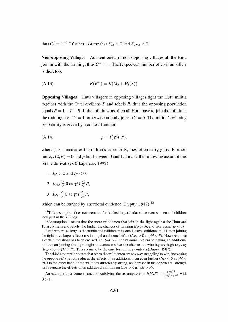
thus C j = 1.41 I further assume that KM > 0 and KMM < 0.
Non-opposing Villages As mentioned, in non-opposing villages all the Hutujoin in with the training, thus Cw = 1. The (expected) number of civilian killersis therefore
(A.13) E(Kw) = K(Me +Ml(S)).
Opposing Villages Hutu villagers in opposing villages fight the Hutu militiatogether with the Tutsi civilians T and rebels R, thus the opposing populationequals P = 1+T +R. If the militia wins, then all Hutu have to join the militia inthe training, i.e. Co = 1, otherwise nobody joins, Co = 0. The militia’s winningprobability is given by a contest function
(A.14) p = I(γM,P),
where γ > 1 measures the militia’s superiority, they often carry guns. Further-more, I(0,P) = 0 and p lies between 0 and 1. I make the following assumptionson the derivatives (Skaperdas, 1992)
1. IM > 0 and IP < 0,
2. IMM T 0 as γM S P,
3. IMP S 0 as γM S P,
which can be backed by anecdotal evidence (Dupuy, 1987).42
41This assumption does not seem too far fetched in particular since even women and childrentook part in the killings.
42Assumption 1 states that the more militiamen that join in the fight against the Hutu andTutsi civilians and rebels, the higher the chances of winning (IM > 0), and vice versa (IP < 0).
Furthermore, as long as the number of militiamen is small, each additional militiaman joiningthe fight has a larger effect on winning than the one before (IMM > 0 as γM < P). However, oncea certain threshold has been crossed, i.e. γM > P, the marginal returns to having an additionalmilitiaman joining the fight begin to decrease since the chances of winning are high anyway(IMM < 0 as γM > P). This seems to be the case for military contexts (Dupuy, 1987).
The third assumption states that when the militiamen are anyway struggling to win, increasingthe opponents’ strength reduces the effects of an additional man even further (IMP < 0 as γM <P). On the other hand, if the militia is sufficiently strong, an increase in the opponents’ strengthwill increase the effects of an additional militiaman (IMP > 0 as γM > P).
An example of a contest function satisfying the assumptions is I(M,P) = (γM)β
(γM)β+Pβwith
β > 1.
A.91
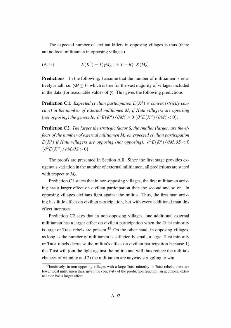
The expected number of civilian killers in opposing villages is thus (thereare no local militiamen in opposing villages)
(A.15) E(Ko) = I(γMe,1+T +R) ·K(Me).
Predictions In the following, I assume that the number of militiamen is rela-tively small, i.e. γM ≤ P, which is true for the vast majority of villages includedin the data (for reasonable values of γ). This gives the following predictions
Prediction C 1. Expected civilian participation E(K j) is convex (strictly con-
cave) in the number of external militiamen Me if Hutu villagers are opposing
(not opposing) the genocide: ∂ 2E(Ko)/∂M2e ≥ 0
(∂ 2E(Kw)/∂M2
e < 0).
Prediction C2. The larger the strategic factor S, the smaller (larger) are the ef-
fects of the number of external militiamen Me on expected civilian participation
E(K j) if Hutu villagers are opposing (not opposing): ∂ 2E(Ko)/∂Me∂S < 0(∂ 2E(Kw)/∂Me∂S > 0
).
The proofs are presented in Section A.8. Since the first stage provides ex-ogenous variation in the number of external militiamen, all predictions are statedwith respect to Me.
Prediction C1 states that in non-opposing villages, the first militiaman arriv-ing has a larger effect on civilian participation than the second and so on. Inopposing villages civilians fight against the militia. Thus, the first man arriv-ing has little effect on civilian participation, but with every additional man thiseffect increases.
Prediction C2 says that in non-opposing villages, one additional externalmilitiaman has a larger effect on civilian participation when the Tutsi minorityis large or Tutsi rebels are present.43 On the other hand, in opposing villages,as long as the number of militiamen is sufficiently small, a large Tutsi minorityor Tutsi rebels decrease the militia’s effect on civilian participation because 1)the Tutsi will join the fight against the militia and will thus reduce the militia’schances of winning and 2) the militiamen are anyway struggling to win.
43Intuitively, in non-opposing villages with a large Tutsi minority or Tutsi rebels, there arefewer local militiamen thus, given the concavity of the production function, an additional exter-nal man has a larger effect.
A.92

A.7.2 Results
Prediction C1: Functional Form Supporting the obedience channel, the ef-fects of an additional militiaman seem to be decreasing. The concave relation-ship between civilian perpetrators and militiamen is presented graphically inFigure A.21, using nonparametric local mean smoothing with an Epanechnikovkernel, conditional on the controls from my preferred specification (regression 6in Panel B in Table 3 in the paper) and instrumenting for the number of militia-men. Furthermore, when I regress civilian participation (residuals) on a second-order polynomial in the militiamen residuals from Figure A.21, the square termis negative and highly significant at the 99 percent level, again confirming theconcave relationship.44 The coefficient on the square term is graphically de-picted in Figure A.22, to the far right of the x-axis, labeled Full (sample).45
However, the result must be taken with a pinch of salt since the nonlin-earities in the second stage might be driven by nonlinearities in the first stage.Reassuringly though, the first-stage relationship looks reasonably linear.46
Prediction C1: Interaction Effects Note that the results shown in SectionA.6 (Table A.31) clearly support the obedience channel: the effect of the militiais larger in places with Tutsi Rebels and a strong Tutsi minority. Besides, furtherconsistent with the model, the effects seem to be weaker in places with RTLMcoverage.47
Identifying Opposing Villages The empirical evidence suggests that the mili-tiamen functioned as a moral authority for the whole sample of villages and thebulk of anecdotal evidence supports this view. The same anecdotal evidence,
44The concave relationship might simply mirror differences in militia quality. For in-stance, extremely successful militiamen might have been operating in small groups whereasthe badly-trained/badly-equipped militia might have moved around in larger groups (with somewell-trained men to guide them). However, since anecdotal evidence suggests that the well-trained/well-equipped troops often led the larger operations which resulted in massive killings,I drop those villages with mass graves and rerun the analysis. Importantly, the effects are stillequally concave (Figure A.25 in Section A.7.3 below).
45Restricting the sample to those villages where militiamen make up less than 5 percent orless than 2.5 percent of the population, i.e. where γM ≤ P, still delivers equally concave effects(Figures A.23 and A.24 in Section A.7.3 below).
46Figure A.26 in Section A.7.3.47RTLM coverage increases the number of local militia men and thus reduces the marginal
effect of an additional external militia member.
A.93

however, also suggests that in some villages civilians did oppose the militia.Identifying those, potentially few, villages is not only interesting in itself butalso allows me to test the predictions of the force model. In particular, anecdo-tal evidence suggests that villages with a large proportion of ethnically mixedhouseholds were more likely to oppose the militia, since civilians would be morewilling to resist when their family members’ and friends’ lives were at risk (DesForges, 1999).
Summing up over all Hutu and Hutu-Tutsi households Fc in a commune c
(remember that ethnicity data is only available at the commune level), I defineintra-household ethnic polarization as48
(A.16) IHEPc =Fc
∑i=1
Nic
Nc·hic · tic,
where Nc is the total number of people in all households Fc in commune c, Nic
the number of people in household i and hic is the fraction of household mem-bers in household i that are Hutu and tic the fraction that are Tutsi, respectively.The higher this measure is, the higher the chances that civilians in those villagesopposed the militia.
In Figure A.22 I report the coefficients on the square term from regressionsof civilian participation (residuals, netting out all controls) on a second-orderpolynomial in the militiamen residuals from Figure A.21, for different per-centiles of intra-household ethnic polarization. Interestingly, for villages withhigh levels of intra-household ethnic polarization (up to the 91st percentile), i.e.those where one would expect resistance, the effects of an additional militiamanare increasing (the point estimates on the square term are positive and signifi-cant), as predicted by the force model (Prediction C2). From the 90th percentileonwards, point estimates turn insignificant and finally negative for the full sam-ple of villages.49
Furthermore, anecdotal evidence suggests that these villages with high lev-
48Note that I do not include pure-Tutsi households. The reason is that pure-Tutsi householdswould reduce the polarization measure, since it is symmetric, but they do not reduce the likeli-hood of opposition.
49The convex relationship between civilian perpetrators and militiamen for high levels ofintra-household ethnic polarization is also presented graphically in Figure A.27 in Section A.7.3below. However, sample sizes are small and the results should therefore again be interpretedwith caution.
A.94

els of intra-household ethnic polarization were opposing the genocide. For ex-ample, Des Forges (1999) writes that in Huye commune (97th percentile), bothHutu and Tutsi civilians fended off attackers from outside. Des Forges (1999, p.350) continues that a witness from the commune of Ngoma (98th percentile) re-calls that “Kanyabashi (the burgomaster) urged the people of Cyarwa to avoid
violence and to fight together against attacks.” On a more general note, many ofthe communes with high intra-household polarization are located in the south-west of Rwanda, where the opposition was overall more pronounced.
References
[1] Des Forges, A. 1999. Leave None to Tell the Story: Genocide in Rwanda,New York: Human Rights Watch.
[2] Dupuy, T. N. 1987. Understanding War, New York: Paragon House.
[3] Skaperdas, S. 1992. Cooperation, Conflict and Power in the Absence ofProperty Rights, American Economic Review, 82(4): 720-739.
A.95
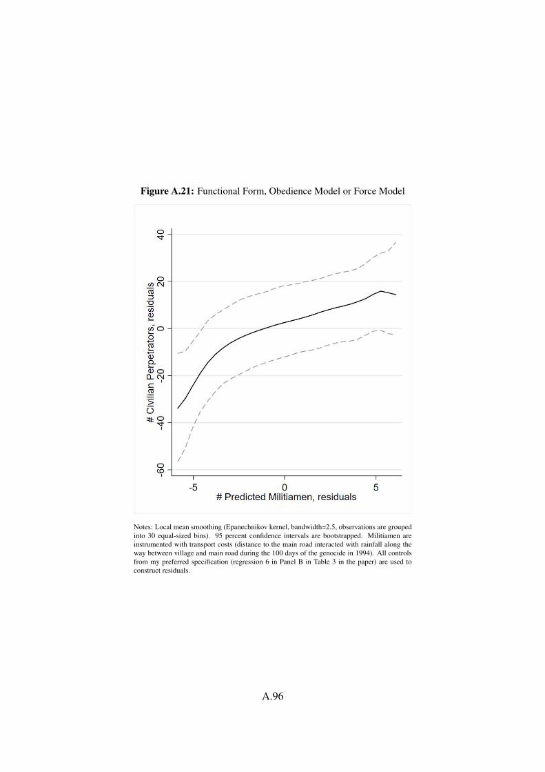
Figure A.21: Functional Form, Obedience Model or Force Model
Notes: Local mean smoothing (Epanechnikov kernel, bandwidth=2.5, observations are groupedinto 30 equal-sized bins). 95 percent confidence intervals are bootstrapped. Militiamen areinstrumented with transport costs (distance to the main road interacted with rainfall along theway between village and main road during the 100 days of the genocide in 1994). All controlsfrom my preferred specification (regression 6 in Panel B in Table 3 in the paper) are used toconstruct residuals.
A.96
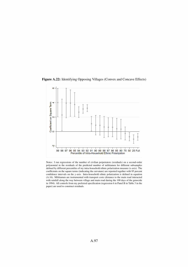
Figure A.22: Identifying Opposing Villages (Convex and Concave Effects)
Notes: I run regressions of the number of civilian perpetrators (residuals) on a second-orderpolynomial in the residuals of the predicted number of militiamen for different subsamplesdefined by different percentiles of my intra-household ethnic polarization measure (x-axis). Thecoefficients on the square terms (indicating the curvature) are reported together with 95 percentconfidence intervals on the y-axis. Intra-household ethnic polarization is defined in equation(A.16). Militiamen are instrumented with transport costs (distance to the main road interactedwith rainfall along the way between village and main road during the 100 days of the genocidein 1994). All controls from my preferred specification (regression 6 in Panel B in Table 3 in thepaper) are used to construct residuals.
A.97

A.7.3 Additional Figures and Tables
Figure A.23: Functional Form (# Militiamen/Population ≤ 5 percent)
Notes: Local mean smoothing (Epanechnikov kernel, bandwidth=2.5, observations are groupedinto 30 equal-sized bins). 95 percent confidence intervals are bootstrapped. Militiamen areinstrumented with transport costs (distance to the main road interacted with rainfall along theway between village and main road during the 100 days of the genocide in 1994). All controlsfrom my preferred specification (regression 6 in Panel B in Table 3 in the paper) are used toconstruct residuals. The sample is restricted to villages where militiamen make up less than 5percent of the village population.
A.98
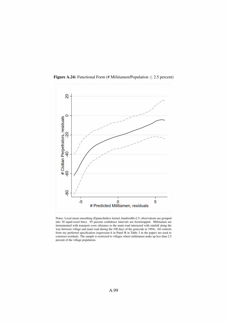
Figure A.24: Functional Form (# Militiamen/Population ≤ 2.5 percent)
Notes: Local mean smoothing (Epanechnikov kernel, bandwidth=2.5, observations are groupedinto 30 equal-sized bins). 95 percent confidence intervals are bootstrapped. Militiamen areinstrumented with transport costs (distance to the main road interacted with rainfall along theway between village and main road during the 100 days of the genocide in 1994). All controlsfrom my preferred specification (regression 6 in Panel B in Table 3 in the paper) are used toconstruct residuals. The sample is restricted to villages where militiamen make up less than 2.5percent of the village population.
A.99

Figure A.25: Functional Form (Excluding Villages with Mass Graves)
Notes: Local mean smoothing (Epanechnikov kernel, bandwidth=2.5, observations are groupedinto 30 equal-sized bins). 95 percent confidence intervals are bootstrapped. Militiamen areinstrumented with transport costs (distance to the main road interacted with rainfall along theway between village and main road during the 100 days of the genocide in 1994). All controlsfrom my preferred specification (regression 6 in Panel B in Table 3 in the paper) are used toconstruct residuals. The sample is restricted to villages where no mass grave was found.
A.100

Figure A.26: Linear First-Stage Relationship
Notes: Local nonparametric estimation (Epanechnikov kernel, bandwidth=0.7, observations are grouped into 100 equal-sized bins). Armed Groups’ Transport Cost is the instrument (distance to the main road interacted with rainfall alongthe way between village and main road during the 100 days of the genocide in 1994). All controls from my preferredspecification (regression 3 in Panel A in Table 3 in the paper) are used to construct residuals.
A.101

Figure A.27: Opposing Villages (Convex Effects)
Notes: Y-axis: # Civilian Perpetrators, residuals. X-axis: # Predicted Militiamen, residuals. Local mean smoothing(Epanechnikov kernel, bandwidth=3). 95 percent confidence intervals are bootstrapped. Samples restricted to 98th, 97thand 95th percentile of intra-household ethnic polarization. Intra-household ethnic polarization is defined in equation(A.9) in the paper. Militiamen are instrumented with transport costs (distance to the main road interacted with rainfallalong the way between village and main road during the 100 days of the genocide in 1994). All controls from mypreferred specification (regression 6 in Panel B in Table 3 in the paper) are used to construct residuals.
A.102

A.8 Proofs
Prediction C1 – Functional Form
1. Non-opposing Villages: The result follows directly from the assumption thatKMM < 0.
2. (i) Opposing Villages, γM ≤ 1 + T + R: Since the second derivative ofH(M,P) = I(M,P) ·K(M) involves KMM < 0, which is negative, the result doesnot follow directly from differentiation. To show that H(M,P) is convex in M
note that convexity of I(M,P) implies that for any two points M1≥ 0 and M2≥ 0and λ between 0 and 1, we have
(A.17) λ I(M1)+ (1−λ )I(M2) ≥ I(λM1 +(1−λ )M2).
Now, set M2 = 0. This gives
(A.18) λ I(M1) ≥ I(λM1).
Multiply both sides by K(M1) ≥ 0 to get
(A.19) λ I(M1) ·K(M1) ≥ I(λM1) ·K(M1).
Note that since K(M) is strictly increasing
(A.20) λ I(M1) ·K(M1) ≥ I(λM1) ·K(M1) > I(λM1) ·K(λM1).
Rearranging gives
(A.21) λH(M1) > H(λM1),
which implies convexity of H.
2. (ii) Opposing Villages, γM > 1 + T + R: Since both I(M,P) and K(M)
are concave functions once γM > P, the curvature of the product of the two isambiguous and depends on functional forms. However, since I(M,P) has toapproach 1 and thus I(M,P) · K(M) will approach K(M) the effects eventuallywill turn concave. To illustrate that the product of two concave functions caneither be concave or convex consider I(M,P) = Mα
P (as long as Mα < P) with0 < α < 1 and K(M) = Mβ with 0 < β < 1. The resulting product H(M,P) =Mα+β
P is convex if α +β ≥ 1 but strictly concave otherwise.
A.103

Prediction C2 – Interactions
1. Non-opposing Villages: Take the derivative of E (Kw) w.r.t. S and Me to get
(A.22)∂E (Kw)
∂S∂Me= KMM(Me +Ml(S)) ·
∂Ml
∂S.
The result follows immediately, since both terms in the product are negative.
2. (i) Opposing Villages, γM ≤ 1+T +R: Take the derivative of E (Ko) w.r.t.S and Me = M to get
(A.23)∂E (Ko)
∂S∂M= IMP(M,P) ·K(M)+ IP(M,P) ·KM(M).
The result follows immediately, since the first term in the sum is non-positiveand the second term is negative.
2. (ii) Opposing Villages, γM > 1+T +R: Now IMP(M,P) > 0, thus ∂E(Ko)∂S∂M
in equation (A.23) is ambiguous.
A.104