One billion Euro program for early childcareservices in Italy*

Isabella Giorgettia† and Matteo Picchioa,b,c,d

a Department of Economics and Social Sciences, Marche Polytechnic University, Italyb Sherppa, Ghent University, Belgium

c IZA, Germanyd GLO

July 30, 2018

Abstract

In 2007 the Italian central government started a program by transferring fundsto regional governments to develop both private and public early childcare services.Exploiting the different timing of program implementation across regions, we eval-uate its effectiveness in boosting the public supply of early childhood educationalservices. We find that the ratio between the available slots in public early childhoodeducation and the population of those aged 0-2 increased by 18.1% three years afterthe start of the program, with respect to the pre-program level. The program impactwas however nil in the South and totally driven by the Center-North.

Keywords: Early childcare services, public early childhood education, governmenttransfers, difference-in-differencesJEL classification codes: C23, H52, H70, J13, R10

*We wish thank Barbara Ermini, Daniele Ripanti, and Raffaella Santolini for their help with the data.†Corresponding author: Department of Economics and Social Sciences, Marche Polytechnic

University, Ancona, 60121, Italy. E-mail addresses: i.giorgetti@univpm.it (I. Giorgetti);m.picchio@univpm.it (M. Picchio).

1 Introduction

Over the last decades, European policy-makers’ agenda has supported the increase infemale labour force participation (FLFP) as one of the most crucial goals to reach. Fromthe Lisbon Strategy (CEU, 2000) to the Europe 2020 Strategy of Smart, Sustainable andInclusive Growth (European Commission, 2010), the targets of female employment ratewere set respectively to 60% and to 75% in the European Union. To favor this strategy,in particular to boost maternal employment, Barcelona European Council (CEU, 2002)established that early childcare provision should reach at least 33% of children underthree years of age, especially in Southern countries where early childcare facilities havebeen scarce.

Early studies showed that female labour supply is elastic to childcare access and itscost,1 so that childcare subsidies were important in encouraging FLFP (Blau and Robins,1988; Ribar, 1995; Blau, 2003). The meta-analysis in Akgunduz and Plantenga (2018)however revealed that labour supply elasticities became somewhat smaller over time andthat they were insignificant in some countries. They claimed that this heterogeneity acrosscountries might be due to different institutions. In countries with high FLFP, high part-time rates, and/or already highly subsidized childcare systems like Norway, France, theNetherlands, and Sweden, policies expanding subsidized child care had a weak effect onmaternal employment (Lundin et al., 2008; Havnes and Mogstad, 2011; Givord and Mar-bot, 2015; Bettendorf et al., 2015), but rather crowded out informal child care arrange-ments. In countries like Germany, Italy, and Belgium, where childcare is “rationed”,2 ma-ternal employment is instead mainly affected by an increase in the supplied slots of earlychildhood education, with price reductions playing a secondary role (Wrohlich, 2004;Del Boca and Vuri, 2007; Valdelanoote et al., 2015). The impact of childcare access andprices on FLFP was also found to be heterogeneous across subpopulations: the laboursupply of low-income, single, and low-educated mother was more responsive to childcareaccess and prices (Del Boca et al., 2009; Akgunduz and Plantenga, 2018).

Empirical studies for Italy pointed out that making it easier to access early childcareservices would be very effective in allowing households to reconcile family and work(Del Boca, 2002; Bratti et al., 2005; Del Boca et al., 2005; Del Boca and Vuri, 2007; DelBoca and Sauer, 2009). Brilli et al. (2016) found indeed that an increase by one percent inpublic childcare coverage raised maternal employment by 1.3 percentage points, with thisimpact being larger in provinces with lower childcare availability. Figari and Narazani

1See Blau and Currie (2006) and Akgunduz and Plantenga (2018) for recent reviews.2In these countries, the demand of slots in public early childcare education exceeds their supply. Local

authorities set therefore eligibility criteria and this selection process is known as “rationing”.

1

(2017) estimated a joint structural model of Italian female labour supply and childcarebehaviour including choices in formal or informal childcare services. They found thatincreasing childcare coverage rate of formal care is more effective than decreasing thecosts in encouraging FLFP.

The Italian government, in order to catch up with the European target (CEU, 2002)about the local coverage of early childcare services and to increase the FLFP,3 startedwith the 2007 Budget Law (Law 296/2006) a three-year special public plan, called “PianoStraordinario per lo Sviluppo dei Servizi per la Prima Infanzia” (PSSSPI). The programwas further extended in 2010, 2012, and 2014, for a total public expenditure of about e1billion. The funds were allocated to regional governments in order to subsidize the de-velopment of both public and private early childcare services. The regional governmentswere asked to co-finance the transfer from the national government. Public and privatechildcare providers, among which also municipalities, had to apply to obtain the subsidyfrom their own regions.

The e1 billion program was expected to be effective in increasing maternal employ-ment to the extent to which the transfers were actually and efficiently used in expandingthe supply of childcare services. Furthermore, in order to boost the employment rate ofmothers belonging to disadvantaged groups, the transfers should have been able to expandthe supply of inexpensive childcare services, typically public early childhood educationalservices. Our study aims at evaluating the impact of PSSSPI on the availability of slots inpublic early childhood educational services. This is of utmost importance. If the impactis weak or nil, we cannot expect effects on maternal employment. Moreover, in general,it cannot be given for granted that large transfers from the central governments to localauthorities are able to generate the expected impact. There might be several reasons todoubt about the efficient use of government funds when transferred to local authorities.The effectiveness of transfers from the central government to local administrations couldbe limited, for example, by the poor functioning of local institutions in the administrationsof the resources or by distorting mechanisms in political economy, such that additionalresources increase political corruption and politicians grabbing rents from the transfers(Brollo et al., 2013). About the former, Bandiera et al. (2009) found that in Italy morethan 80% of the public waste is related to an inefficient administration of the transfersfrom the central government. About the latter, there is evidence for Italy of biases in theallocation and use of central transfers: i) Barone and Narciso (2013) detected connectionsbetween the local presence of organized crime and the amount of public funding trans-

3The Italian FLFP and the female employment rates (15-64 years) are still away from the achievementof the targets set by European Commission (2010). In 2015 they were 55.9% and by 47.2% , respectively(Eurostat, Labour Force Survey).

2

ferred from the central government; ii) Carozzi and Repetto (2016) showed that transfersto municipalities depend on the birth town of the members of Parliament, rather than ex-clusively on local development needs; iii) De Angelis et al. (2018) found that white collarcrimes increased in the South in the presence of EU disbursements.

The main difficulty in identifying the impact of a nationwide policy intervention con-sists in disentangling its true effect from the spurious one related to the time trend. How-ever, the transfers to the regions did not take place at the same moment. Regions hadindeed to pass a set of acts to receive the transfers from the central government. Theyneeded to update their legislation about the different types of early childcare services andto design the executive authorizing procedures for transferring grants to the final child-care service providers (Istituto degli Innocenti, 2009). The different timing with which thefunds were transferred from the central government to the regions were plausibly exoge-nous with respect to the level of supply of slots in public early childhood education at thelocal level. The implementation timing is indeed likely to be determined by the level ofadministrative capacity of the regional bureaucracy, as reported by Soncin (2013, p. 73).Consistently, while studying the determinants of the performance of Italian regions inspending resources from European structural funds, Milio (2007) showed that the delaysin the programmatic acts to spend their allocated resources were due to their own admin-istrative capacity. Exploiting the different timing of transfers across the Italian regions,we estimate, in a Difference-in-Differences (DiD) model, the causal impact of PSSSPIon the coverage rate of public early childcare services, defined as the ratio between theavailable number of slots in public early childhood education and the population aged0-2 (up to 36 months of age). The empirical analysis is based on a dataset at municipallevel collected by the Italian Department of Territorial and Internal Affairs over the years2004-2013 and containing, among other variables, also information on local public formalchildcare supply.

We find that the PSSSPI was effective in increasing the ratio between the availableslots in public early childhood education and the population of those aged 0-2: withrespect to the pre-program average coverage rate, it increased by 5.5% in the year ofintervention and by 18.1% three years after the start of the program. The effect wasnot however homogeneous across regions. Even if the Southern regions were asked toco-finance the transfers from the national government more heavily, no increase in thecoverage rate is detected in the Southern regions. On the contrary, in the Center-North,the increase in the coverage rate amounted to 12.7% in the year of intervention and by32.1% three years after the beginning of the program. Finally, we found that the programhad positive effects on the coverage rate in the Center-North both in the provincial capitalsand in the rest of the territory.

3

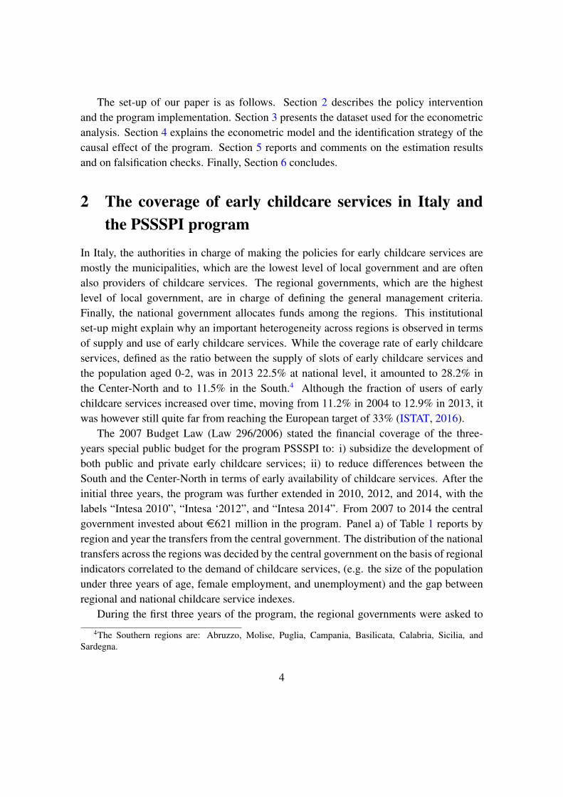
The set-up of our paper is as follows. Section 2 describes the policy interventionand the program implementation. Section 3 presents the dataset used for the econometricanalysis. Section 4 explains the econometric model and the identification strategy of thecausal effect of the program. Section 5 reports and comments on the estimation resultsand on falsification checks. Finally, Section 6 concludes.

2 The coverage of early childcare services in Italy andthe PSSSPI program

In Italy, the authorities in charge of making the policies for early childcare services aremostly the municipalities, which are the lowest level of local government and are oftenalso providers of childcare services. The regional governments, which are the highestlevel of local government, are in charge of defining the general management criteria.Finally, the national government allocates funds among the regions. This institutionalset-up might explain why an important heterogeneity across regions is observed in termsof supply and use of early childcare services. While the coverage rate of early childcareservices, defined as the ratio between the supply of slots of early childcare services andthe population aged 0-2, was in 2013 22.5% at national level, it amounted to 28.2% inthe Center-North and to 11.5% in the South.4 Although the fraction of users of earlychildcare services increased over time, moving from 11.2% in 2004 to 12.9% in 2013, itwas however still quite far from reaching the European target of 33% (ISTAT, 2016).

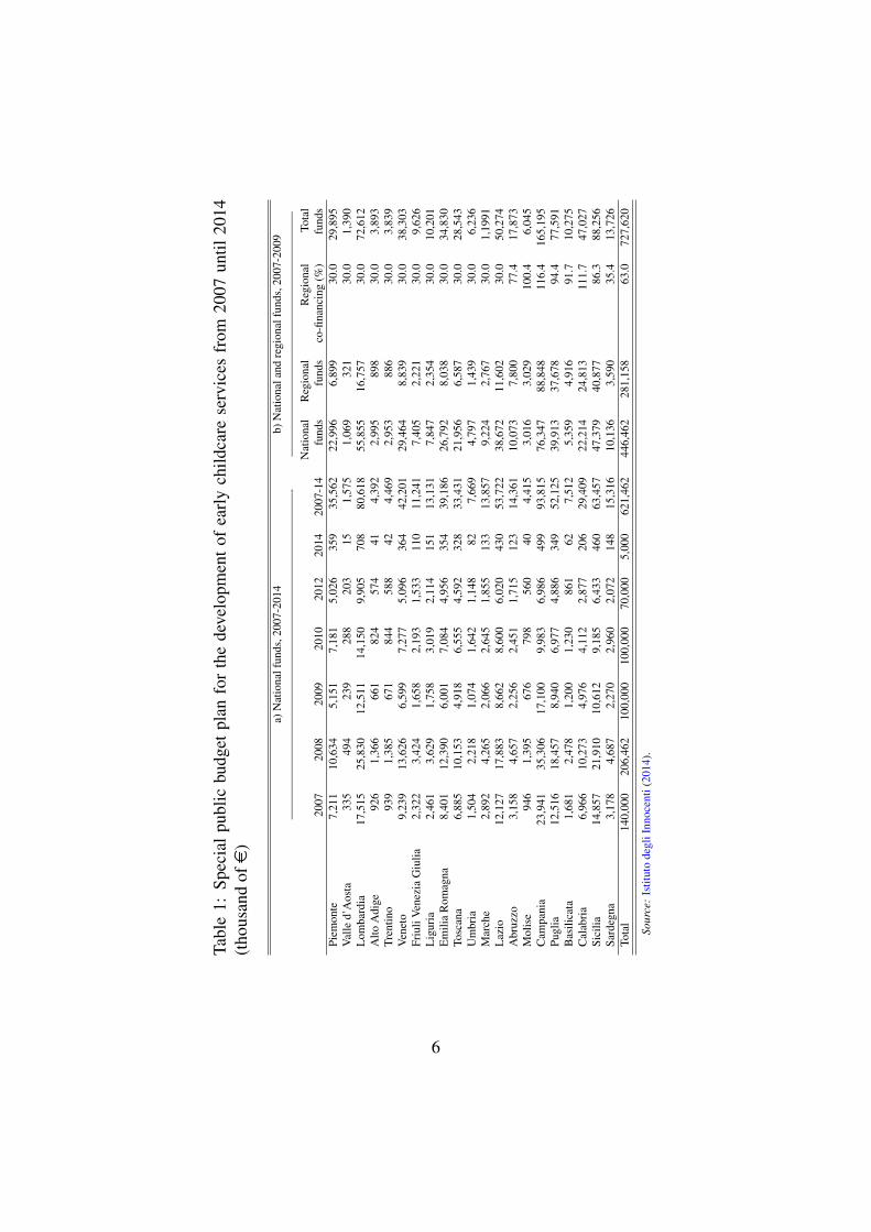
The 2007 Budget Law (Law 296/2006) stated the financial coverage of the three-years special public budget for the program PSSSPI to: i) subsidize the development ofboth public and private early childcare services; ii) to reduce differences between theSouth and the Center-North in terms of early availability of childcare services. After theinitial three years, the program was further extended in 2010, 2012, and 2014, with thelabels “Intesa 2010”, “Intesa ‘2012”, and “Intesa 2014”. From 2007 to 2014 the centralgovernment invested about e621 million in the program. Panel a) of Table 1 reports byregion and year the transfers from the central government. The distribution of the nationaltransfers across the regions was decided by the central government on the basis of regionalindicators correlated to the demand of childcare services, (e.g. the size of the populationunder three years of age, female employment, and unemployment) and the gap betweenregional and national childcare service indexes.

During the first three years of the program, the regional governments were asked to

4The Southern regions are: Abruzzo, Molise, Puglia, Campania, Basilicata, Calabria, Sicilia, andSardegna.

4

co-finance the intervention, with a total contribution of almost e300 million. Centraland Northern regions had to co-sponsor 30% of the national transfer. Southern regions,in which the supply of early childcare services was especially low, had instead to give alarger contribution, which went from 35.4% for Sardegna to 116.4% for Campania. Panelb) of Table 1 reports the national and regional funds in the first three years of the program,as well as the regional co-sponsoring rate.

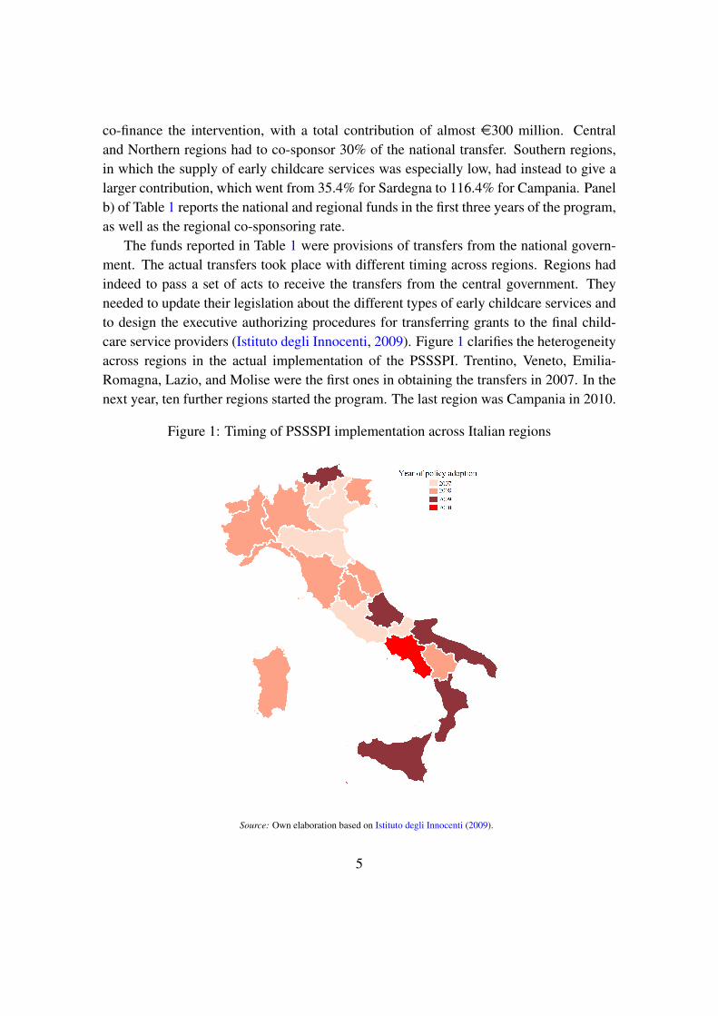
The funds reported in Table 1 were provisions of transfers from the national govern-ment. The actual transfers took place with different timing across regions. Regions hadindeed to pass a set of acts to receive the transfers from the central government. Theyneeded to update their legislation about the different types of early childcare services andto design the executive authorizing procedures for transferring grants to the final child-care service providers (Istituto degli Innocenti, 2009). Figure 1 clarifies the heterogeneityacross regions in the actual implementation of the PSSSPI. Trentino, Veneto, Emilia-Romagna, Lazio, and Molise were the first ones in obtaining the transfers in 2007. In thenext year, ten further regions started the program. The last region was Campania in 2010.

Figure 1: Timing of PSSSPI implementation across Italian regions

Source: Own elaboration based on Istituto degli Innocenti (2009).

5

Tabl

e1:

Spec

ialp

ublic

budg

etpl

anfo

rth

ede

velo

pmen

tof

earl

ych

ildca

rese

rvic

esfr

om20

07un

til20

14(t

hous

and

ofe

)

a)N

atio

nalf

unds

,200

7-20

14b)

Nat

iona

land

regi

onal

fund

s,20

07-2

009

——

——

——

——

——

——

——

——

——

——

——

——

——

——

-—

——

——

——

——

——

——

——

——

——

——

Nat

iona

lR

egio

nal

Reg

iona

lTo

tal

2007

2008

2009

2010

2012

2014

2007

-14

fund

sfu

nds

co-fi

nanc

ing

(%)

fund

sPi

emon

te7,

211

10,6

345,

151

7,18

15,

026

359

35,5

6222

,996

6,89

930

.029

,895

Val

led’

Aos

ta33

549

423

928

820

315

1,57

51,

069

321

30.0

1,39

0L

omba

rdia

17,5

1525

,830

12,5

1114

,150

9,90

570

880

,618

55,8

5516

,757

30.0

72,6

12A

ltoA

dige

926

1,36

666

182

457

441

4,39

22,

995

898

30.0

3,89

3Tr

entin

o93

91,

385

671

844

588

424,

469

2,95

388

630

.03,

839

Ven

eto

9,23

913

,626

6,59

97,

277

5,09

636

442

,201

29,4

648,

839

30.0

38,3

03Fr

iuli

Ven

ezia

Giu

lia2,

322

3,42

41,

658

2,19

31,

533

110

11,2

417,

405

2,22

130

.09,

626

Lig

uria

2,46

13,

629

1,75

83,

019

2,11

415

113

,131

7,84

72,

354

30.0

10,2

01E

mili

aR

omag

na8,

401

12,3

906,

001

7,08

44,

956

354

39,1

8626

,792

8,03

830

.034

,830

Tosc

ana

6,88

510

,153

4,91

86,

555

4,59

232

833

,431

21,9

566,

587

30.0

28,5

43U

mbr

ia1,

504

2,21

81,

074

1,64

21,

148

827,

669

4,79

71,

439

30.0

6,23

6M

arch

e2,

892

4,26

52,

066

2,64

51,

855

133

13,8

579,

224

2,76

730

.01,

1991

Laz

io12

,127

17,8

838,

662

8,60

06,

020

430

53,7

2238

,672

11,6

0230

.050

,274

Abr

uzzo

3,15

84,

657

2,25

62,

451

1,71

512

314

,361

10,0

737,

800

77.4

17,8

73M

olis

e94

61,

395

676

798

560

404,

415

3,01

63,

029

100.

46,

045

Cam

pani

a23

,941

35,3

0617

,100

9,98

36,

986

499

93,8

1576

,347

88,8

4811

6.4

165,

195

Pugl

ia12

,516

18,4

578,

940

6,97

74,

886

349

52,1

2539

,913

37,6

7894

.477

,591

Bas

ilica

ta1,

681

2,47

81,

200

1,23

086

162

7,51

25,

359

4,91

691

.710

,275

Cal

abri

a6,

966

10,2

734,

976

4,11

22,

877

206

29,4

0922

,214

24,8

1311

1.7

47,0

27Si

cilia

14,8

5721

,910

10,6

129,

185

6,43

346

063

,457

47,3

7940

,877

86.3

88,2

56Sa

rdeg

na3,

178

4,68

72,

270

2,96

02,

072

148

15,3

1610

,136

3,59

035

.413

,726

Tota

l14

0,00

020

6,46

210

0,00

010

0,00

070

,000

5,00

062

1,46

244

6,46

228

1,15

863

.072

7,62

0

Sour

ce:

Istit

uto

degl

iInn

ocen

ti(2

014)

.

6

The final beneficiaries of the program are providers of early childcare services. Theycould be both private and public entities. Typical beneficiaries of the program were mu-nicipalities and private entities supplying daycare centers and supplementary services for0-2 years old children.

3 Data and sample

For the empirical analysis, the main data source is the dataset on local public financecollected by Italian Department of Territorial and Internal Affairs over the years 2004-2013.5 This dataset contains information on demographics, public finance (tax revenuesand expenditures), and public individual-demand services (such as public and financed bypublic funds daycare centers and school canteens) for all the 8,092 Italian municipalities.In particular, we have information on the number of available slots in public and publicfinanced early childhood education. A secondary data source, still at municipality level,concerns information on the population size by age categories, including the group 0-2, obtained by the National Institute of Statistics (Istat).6 Finally, our third data sourcecomes from Istat as well: the regional time series of real GDP growth rate and femaleemployment rate, which will be used as time-varying controls.

After deleting from the sample 7 municipalities on the regional borders which switchedregions in 2009,7 we aggregated the variables at municipality level at the level of provinces.There are 110 provinces in Italy and they are the intermediate level of local governmentbetween the municipalities and regions. Regions are composed of a certain number ofprovinces which, in turn, are made up of a certain number of municipalities. This impliesthat each province belongs to one and only one region. After grouping the data at the levelof provinces, we have a balanced panel of 1,100 observations, over 10 years and across110 provinces.

The outcome variable of primary interest is the coverage rate, defined as the ratiobetween the available slots of public (or financed by public grants) early childhood ed-ucational services in a province and the population aged 0-2 in the same province. Wegrouped the data at the level of provinces for three main reasons. First, most of the mu-nicipalities in Italy are small in terms of population and have therefore no public childcareservice. For example, in 2007 more than 70% of the municipalities had less than 5,000

5See Finanza Locale website on http://finanzalocale.interno.gov.it/apps/floc.php/in/cod/4.6Information on population from 2004 until 2012 comes from the “Atlante Statistico dei Comuni”. For

2013, data on population was downloaded from the online archive “Popolazione e Famiglie”.7In 2009, Casteldelci, Maiolo, Novafeltria, Pennabilli, San Leo, Sant’Agata Feltria, and Talamello

passed from Marche to Emilia Romagna, as a consequence of a referendum result in 2006.

7

inhabitants and 94% of them reported a coverage rate equal to 0. Nationwide, the massof municipalities with no public childcare services amounted to 81%. If we have workedat the level of municipalities, we would have had to face this corner solution problem orstick to an evaluation of the effect at the extensive margin. Second, given that there aremany small municipalities with no public childcare services, it is likely that the demandfor public childcare services of parents living in small municipalities is served by the clos-est large municipality. It might then be that the program will generate an effect only onlarger municipalities, so as to exploit economies of scale and allow all the families of thesurrounding towns to benefit from the enlarged supply of public slots. In other words, wewould consider as treated small municipalities only because they are in a region whichimplemented the program, although the chances that they react to the program are virtu-ally zero, not having the critical size to do it. Third, if the unit of observation were themunicipality, it would be unclear how to weight units in order to take into account the ex-tremely large variability in terms of population (both total and conditional of age) amongmunicipalities and get estimates that could reflect the average impact for a representativemunicipality. For example, in 2007, the median population was 2,424 inhabitants, the99th percentile was 68,739, and 22.7% of the Italian population was concentrated in thetop 0.5% municipalities. Grouping the data at the level of provinces importantly reducesthese problems.

Table 2 reports descriptive statistics of the coverage rate, disaggregated by implemen-tation time, geographical area, and type of municipality. Panel a) of Table 2 shows that,over the ten year time window under analysis, on average in the Italian provinces therewere 8.8 available slots in public early childhood education per 100 children younger than36 months. This figure increased over time: before the policy it amounted to 7.9, whereasit increased by 1.6 points (20%) in the period after the program implementation. Figure2 allows to visually inspect more in detail at the change in the supply of public childcareservices: it clearly shows that the mode shifted to the right, with the right tail becomingfatter.

As we explained in Section 2 and showed in Table 1, the funds were assigned acrossregions taking into account their heterogeneity and needs. More than one half of thenational and regional transfers were indeed used for the 8 regions of the South. In theeconometric analysis we will study this dimension of heterogeneity of the effect. Panel b)of Table 2 reports the coverage rate in the 8 regions of the South and in the rest of Italy,before and after the program implementation. The situation is quite different across theregions. In the South, the coverage rate was 0.041, against 0.118 for the Center-North.The change after the policy seems to be more important in the South, whose coverage rateincreased by about 16%, whereas in the rest of the country it raised by 9%.

8

Table 2: Descriptive statistics of the outcome variable and the timing ofthe program implementation

Mean Std. Dev. Minimum Maximum Observationsa) Coverage rate, whole sample

Coverage rate 0.088 0.060 0.000 0.305 1,100Coverage rate before PSSSPI 0.079 0.055 0.001 0.276 451Coverage rate after PSSSPI 0.095 0.062 0.000 0.305 649

b) Coverage rate, South and Center-NorthCenter-North 0.118 0.057 0.023 0.305 680South 0.041 0.026 0.000 0.110 420Center-North before PSSSPI 0.111 0.052 0.023 0.276 250South before PSSSPI 0.038 0.024 0.001 0.106 201Center-North after PSSSPI 0.121 0.059 0.026 0.305 430South after PSSSPI 0.044 0.027 0.000 0.110 219

c) Coverage rate, provincial capitals and the rest of the territoryCapital 0.146 0.093 0.000 0.462 1,100Not capital 0.069 0.054 0.000 0.277 1,100Capital before PSSSPI 0.132 0.087 0.000 0.435 451Not capital before PSSSPI 0.061 0.050 0.000 0.248 451Capital after PSSSPI 0.156 0.096 0.000 0.462 649Not capital after PSSSPI 0.075 0.056 0.000 0.277 649

d) Policy indicators (lags and leads)3 or more years before of adoption 0.210 0.407 0.000 1.000 1,1002 years before of adoption 0.100 0.300 0.000 1.000 1,1001 year before of adoption 0.100 0.300 0.000 1.000 1,100Year of adoption 0.100 0.300 0.000 1.000 1,1001 year after of adoption 0.100 0.300 0.000 1.000 1,1002 years after of adoption 0.100 0.300 0.000 1.000 1,1003 or more years after of adoption 0.290 0.454 0.000 1.000 1,100

9

Figure 2: Kernel(a) density distribution of the coverage rate before and after PSSSPIimplementation

02

46

8D

ensi

ty

0 .05 .1 .15 .2 .25 .3Coverage rate

Coverage rate before PSSSPI Coverage rate after PSSSPI

(a) Epanechnikov kernel function.

10

Panel c) of Table 2 reports the sample means of the coverage rate by focusing first onthe provincial capitals only and then on provinces after excluding their capital. This isa further heterogeneity dimension that we will investigate. The capitals are, aside froma few exceptions, the largest cities of the province in terms of population8 and from theeconomic point of view. It is interesting to evaluate whether the program impact can differbetween capitals and the rest of the provinces. The theory does not provide indeed clear-cut predictions. On the one hand, provincial capitals are attraction poles for childcareservices because of a higher population density and because they absorb workers from thesurrounding small municipalities. If many childcare service providers are already locatedin the capital, it is more likely that they will apply and obtain the program transfers. Onthe other hand, the coverage rate in small municipalities is low, if not zero. The excessof demand for public early childcare services could then be an important leverage forsmall municipalities to request the transfers and develop them. Understanding whether theprogram was effective in developing early childcare services both in provincial capitalsand in the rest of the territory is a valuable piece of information to shed more light on howand to what extent the PSSSPI modified the local supply of public early childcare services.As expected, the coverage rate is larger in capitals (0.146) than elsewhere (0.069). Bothin the capitals and in the rest of the provinces, the coverage rate went up after the programimplementation, respectively by about 18% and 23%. At least from raw statistics, itseems that the supply of public childcare services increased both in larger and smallermunicipalities. The following econometric analysis aims at disentangling the spuriouseffect due to eventual already ongoing positive trends in the coverage rate, from the trueeffect of the program.

Finally, 3 displays summary statistics of the covariates that will be used in the re-gression model. Apart from the regional indicators, we will also control for the regionalfemale employment and the regional real GDP growth to control for time-varying regionalheterogeneity.

4 Method

Identification of the effect of PSSSPI implementation on the coverage rate is attained byexploiting the fact that the program started in the regions with different timing, gradu-ally from 2007 until 2010. Simply comparing provinces before and after the programimplementation is problematic since there may have been many economic and politicalinfluences other than the PSSSPI that affected the supply of early childcare services over

8In the capitals live approximately one third of the Italian population.

11

Table 3: Summary statistics of covariates

Mean Std. Dev. Minimum MaximumRegional female employment rate 0.473 0.112 0.254 0.623Regional real GDP growth rate -0.003 0.025 -0.085 0.048Regions

Piemonte 0.073 0.266 0.000 1.000Valle d’Aosta 0.009 0.095 0.000 1.000Lombardia 0.109 0.312 0.000 1.000Province of Trento 0.009 0.095 0.000 1.000Province of Bolzano 0.009 0.095 0.000 1.000Veneto 0.063 0.244 0.000 1.000Friuli Venezia Giulia 0.036 0.187 0.000 1.000Liguria 0.036 0.187 0.000 1.000Emilia Romagna 0.082 0.274 0.000 1.000Toscana 0.091 0.288 0.000 1.000Umbria 0.018 0.134 0.000 1.000Marche 0.045 0.208 0.000 1.000Lazio 0.045 0.208 0.000 1.000Abruzzo 0.036 0.187 0.000 1.000Molise 0.018 0.134 0.000 1.000Campania 0.045 0.208 0.000 1.000Puglia 0.055 0.227 0.000 1.000Basilicata 0.018 0.134 0.000 1.000Calabria 0.045 0.208 0.000 1.000Sicilia 0.082 0.274 0.000 1.000Sardegna 0.073 0.260 0.000 1.000

Provinces (Total observations) 110 (1,100)

time. Similarly, by focusing on a particular year in a cross-section framework, a simpledifference in the average coverage rate between regions which already implemented theprogram and those which have not done it yet also pauses a problem because there mightbe fundamental differences in the political attention towards childcare services betweenthe two groups of regions. As a result, we employ a DiD estimator and estimate changesin the differences of the coverage rate of public early childcare services between early andlate implementing regions before and after the reform. The identification of causal effectsrequires some assumptions. In what follows, we conduct statistical tests for each of theseassumptions to check whether they are supported by the data.

Our empirical evaluation will be in a panel data framework. We specify the followingmodel for coverage rate y of province i of region r in year t:

yirt = x′irtβ + γr + φt + δ0Irt + δ1Irt−1 + δ2Irt−2 + δ3Irt−3 + uirt, (1)

where

• xirt is the vector containing the time-varying variables, the regional employmentrate and real GDP growth rate of regressors, and β is the conformable vector ofcoefficients.

12

• γr is a set of regional fixed effects. There are 21 regions in our data, hence theyamount to 20 regional indicators.

• φt is a set of year fixed effects.

• (Irt, Irt−1, Irt−2, Irt−3) are the regressors of interest. They are indicator variables.Irt−τ , with τ = 0, 1, 2, is equal to 1 if the program was implemented in region r attime t− τ . Irt−3 is equal to 1 if the program was implemented 3 or more years ago.The parameter δ0 is the effect of the program in the year of implementation; δ1 is theeffect one year after the year of implementation; δ2 and δ3 are the program impacttwo and three or more years after the program implementation, respectively.

• uirt is the error term at the provincial level.

The parameters of Equation (1) are estimated using Ordinary Least Squares (OLS).Inference deserves a special discussion. In our DiD application the identification of thePSSSPI effect is based on variations across regions and years. The regressors of primaryinterest (Irt, Irt−1, Irt−2, Irt−3) are therefore correlated within regions. Proper inferenceshould take this into account. The cluster-robust variance estimator (CRVE) is a simpleway to deal with correlation within-groups (Liang and Zeger, 1986). However, this ap-proach is unbiased only when the number of clusters is large enough and the asymptoticresults can be safely invoked. In our study, the number of regions is just 21. The CRVE istherefore likely to suffer from a small sample bias, resulting in a type I error.9 Cameronet al. (2008) proposed a wild cluster bootstrap-t procedure to get critical values when thenumber of clusters is small. When reporting the estimation results, the presentation ofthe point estimates of the coefficients of (Irt, Irt−1, Irt−2, Irt−3) will be accompanied byp-values based on the wild cluster bootstrap (WCB) procedure by Cameron et al. (2008)with restricted residuals.10

Some assumptions are required for the OLS estimation of the DiD model in Equation(1) to return unbiased estimates of the causal effect of the program implementation.

Assumption 1 (Parallel trend assumption): Conditional on the control variables, provincesin regions which have already implemented the program would have experienced similartrends in the coverage rate as provinces in regions which have not implemented yet theprogram, in the absence of the program.

9See Cameron and Miller (2015) for an overview of the problems in doing inference when the numberof clusters is small.

10In the WCB procedure with restricted residuals, the bootstrap algorithm the model is re-estimatedunder the null hypothesis of no treatment effect. We bootstrapped the residuals 5,000 times using the Webbsix-point distribution as weights (Webb, 2014).

13

Since we cannot observe the counterfactual evolution of the coverage rate in the absenceof the program implementation, this assumption is not testable. However, we can checkwhether it is at least supported by the data before the policy implementation, by testingwhether the provinces were following parallel trends before regions started distributingthe funds. In the same spirit of Autor (2003), we checked this by augmenting Equation(1) by leads of the indicator for the program implementation, from t+1 up to t+5. If thetrend between treated and not treated yet is parallel before the policy implementation, thecoefficients of these further indicators are to be nil. When this is the case, the provinceswere following parallel trends in the coverage rate while approaching the implementationmoment. We report the results of this check in Subsection 5.3.

Assumption 2 (Exogeneity of the timing of program implementation): Conditional on ob-servables, the timing of the implementation is exogenous with respect to the supply andthe demand of public early childhood educational services. Rather, the timing is politi-cally determined.

The timing of program implementation differed across regions because the transfers fromthe central government took place in different moments. In order to be financed, regionshad to pass a set of acts to update their legislation about the different types of early child-care services and to design the executive authorizing procedures for transferring grants tothe final childcare service providers (Istituto degli Innocenti, 2009). The different timingwith which the funds were transferred from the central government was therefore likelydetermined by the level of administrative capacity of the regional bureaucracy (Soncin,2013, p. 73). There is evidence that this also explains the heterogeneity across regionsin spending resources from European structural funds (Milio, 2007). The fact that theSouthern regions, which were the most in need of early childcare services, delayed theprogram implementation also supports Assumption 2: if the timing had been endogenous,one would have expected the opposite.

Assumption 3 (No anticipation): The local authorities were not able to anticipate thePSSSPI implementation.

This assumption would fail if the municipalities or the region itself anticipated the startof the program and decided either to invest more in childcare services before the actualarrival of the transfers or to postpone some planned investment in childcare services, soas to sponsor them with the PSSSPI. The direction of the eventual bias could go in eitherway. To check whether anticipation might be an issue, in Subsection 5.3 we provide arobustness check by removing for all the provinces the year before the program imple-mentation.

14

5 Estimation results

5.1 Baseline estimation results and their heterogeneity across regionsand municipality type

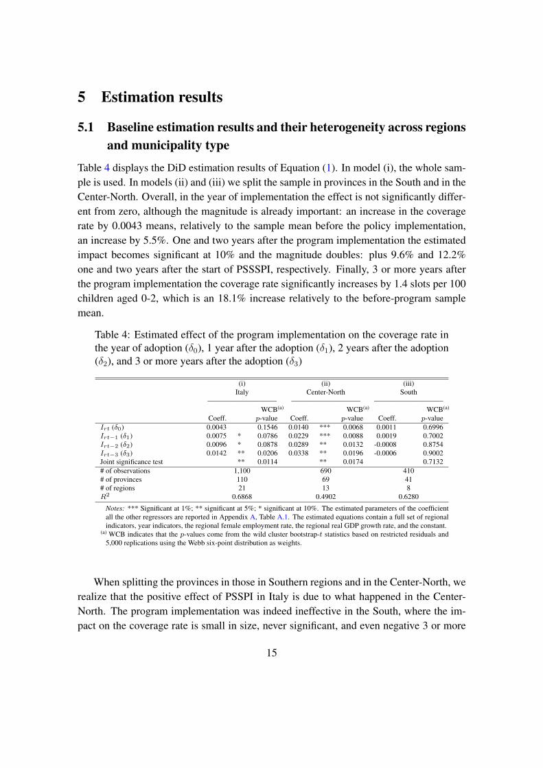
Table 4 displays the DiD estimation results of Equation (1). In model (i), the whole sam-ple is used. In models (ii) and (iii) we split the sample in provinces in the South and in theCenter-North. Overall, in the year of implementation the effect is not significantly differ-ent from zero, although the magnitude is already important: an increase in the coveragerate by 0.0043 means, relatively to the sample mean before the policy implementation,an increase by 5.5%. One and two years after the program implementation the estimatedimpact becomes significant at 10% and the magnitude doubles: plus 9.6% and 12.2%one and two years after the start of PSSSPI, respectively. Finally, 3 or more years afterthe program implementation the coverage rate significantly increases by 1.4 slots per 100children aged 0-2, which is an 18.1% increase relatively to the before-program samplemean.

Table 4: Estimated effect of the program implementation on the coverage rate inthe year of adoption (δ0), 1 year after the adoption (δ1), 2 years after the adoption(δ2), and 3 or more years after the adoption (δ3)

(i) (ii) (iii)Italy Center-North South

—————————– —————————– —————————–WCB(a) WCB(a) WCB(a)

Coeff. p-value Coeff. p-value Coeff. p-valueIrt (δ0) 0.0043 0.1546 0.0140 *** 0.0068 0.0011 0.6996Irt−1 (δ1) 0.0075 * 0.0786 0.0229 *** 0.0088 0.0019 0.7002Irt−2 (δ2) 0.0096 * 0.0878 0.0289 ** 0.0132 -0.0008 0.8754Irt−3 (δ3) 0.0142 ** 0.0206 0.0338 ** 0.0196 -0.0006 0.9002Joint significance test ** 0.0114 ** 0.0174 0.7132# of observations 1,100 690 410# of provinces 110 69 41# of regions 21 13 8R2 0.6868 0.4902 0.6280

Notes: *** Significant at 1%; ** significant at 5%; * significant at 10%. The estimated parameters of the coefficientall the other regressors are reported in Appendix A, Table A.1. The estimated equations contain a full set of regionalindicators, year indicators, the regional female employment rate, the regional real GDP growth rate, and the constant.

(a) WCB indicates that the p-values come from the wild cluster bootstrap-t statistics based on restricted residuals and5,000 replications using the Webb six-point distribution as weights.

When splitting the provinces in those in Southern regions and in the Center-North, werealize that the positive effect of PSSPI in Italy is due to what happened in the Center-North. The program implementation was indeed ineffective in the South, where the im-pact on the coverage rate is small in size, never significant, and even negative 3 or more

15

years after the start of the program. In the provinces in the Center-North, the impact wasimmediate: already in the year of the implementation, the transfers generated a highlysignificant increase in the coverage rate by 1.4 slots in public early childhood educationper 100 children aged 0-2. Relatively to the average coverage rate before the program inthe Center-North, the rise amounts to 12.6%. The impact becomes much stronger whenmoving ahead: 3 or more years after the start of PSSSPI, the coverage rate increases by30.5% with respect to the pre-intervention average.

Finally, we investigated whether the PSSSPI effect could differ between provincialcapitals and the rest of the territory. Panel I) of Table 5 reports the estimate programeffect for the 110 provincial capitals, whilst panel II) focuses on the effect elsewhere.Nationwide, the program increased the supply of public childcare services both in theprovincial capitals and in the rest of the territory, with magnitudes that, relatively to thebefore-program average, are very much the same: 3 (or more) years after the program im-plementation the available slots in public childhood education increased by 19.2% in thecapitals and by 19.6% in the rest of the provinces. This means that the PSSSPI programwas effective also in increasing the supply of public childcare services in smaller townsand less populated areas, where traditionally the availability of public childcare serviceshave been quite scarce.

By splitting the sample of capitals (and of the provinces excluding their capitals) inthose in Southern regions and the ones in the Center-North, we get the same picturecoming from Table 4: the effect is driven by the Center-North and no program effect isdetected in the South, neither in the provincial capitals nor in the rest of the territory.

5.2 Further heterogeneity analysis

In order to have a better understanding of the heterogeneity of the program effect acrossregional differences, we decided to split the sample on the basis of the level of the GDPgrowth rate and of the female employment rate. We looked at the median of these twocovariates in 2004 and split the sample in regions below and above the median GDPgrowth rate and female employment rate. Regions with a high GDP growth rate in 2004might have been more likely to approach the start of the program with more resourceswhich, in turn, might have had a knock-on impact on the effectiveness of the PSSSPI.There are 8 regions with a high GDP growth rate in 2004: 3 from the South (Molise,Calabria, and Sardegna), 2 from the Center (Marche and Lazio), and 3 from the North(Province of Bolzano, Veneto, and Emilia Romagna). The estimation results for model (i)in Table 6 show that, for high GDP growth rate regions, the PSSSPI was effective. Giventhat the coverage rate in the years before the program start in these 8 regions was equal to

16

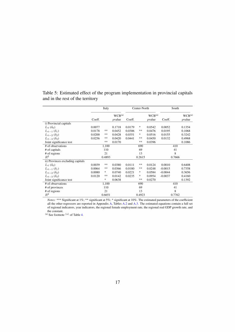
Table 5: Estimated effect of the program implementation in provincial capitalsand in the rest of the territory

Italy Center-North South—————————– —————————– —————————–

WCB(a) WCB(a) WCB(a)

Coeff. pvalue Coeff. pvalue Coeff. pvaluei) Provincial capitalsIrt (δ0) 0.0077 0.1718 0.0179 * 0.0542 0.0052 0.1354Irt−1 (δ1) 0.0178 ** 0.0452 0.0306 ** 0.0476 0.0195 0.1068Irt−2 (δ2) 0.0200 ** 0.0428 0.0351 * 0.0516 0.0155 0.3242Irt−3 (δ3) 0.0256 ** 0.0420 0.0441 ** 0.0450 0.0132 0.4968Joint significance test ** 0.0170 ** 0.0396 0.1086# of observations 1,100 690 410# of capitals 110 69 41# of regions 21 13 8R2 0.4893 0.2615 0.7666ii) Provinces excluding capitalsIrt (δ0) 0.0039 ** 0.0380 0.0111 ** 0.0124 0.0010 0.6408Irt−1 (δ1) 0.0064 ** 0.0366 0.0180 ** 0.0248 -0.0015 0.7358Irt−2 (δ2) 0.0080 * 0.0740 0.0221 * 0.0584 -0.0044 0.3656Irt−3 (δ3) 0.0120 ** 0.0142 0.0235 * 0.0954 -0.0037 0.4160Joint significance test * 0.0638 ** 0.0270 0.1392# of observations 1,100 690 410# of provinces 110 69 41# of regions 21 13 8R2 0.6651 0.4923 0.7762

Notes: *** Significant at 1%; ** significant at 5%; * significant at 10%. The estimated parameters of the coefficientall the other regressors are reported in Appendix A, Tables A.2 and A.3. The estimated equations contain a full setof regional indicators, year indicators, the regional female employment rate, the regional real GDP growth rate, andthe constant.

(a) See footnote (a) of Table 4.

17

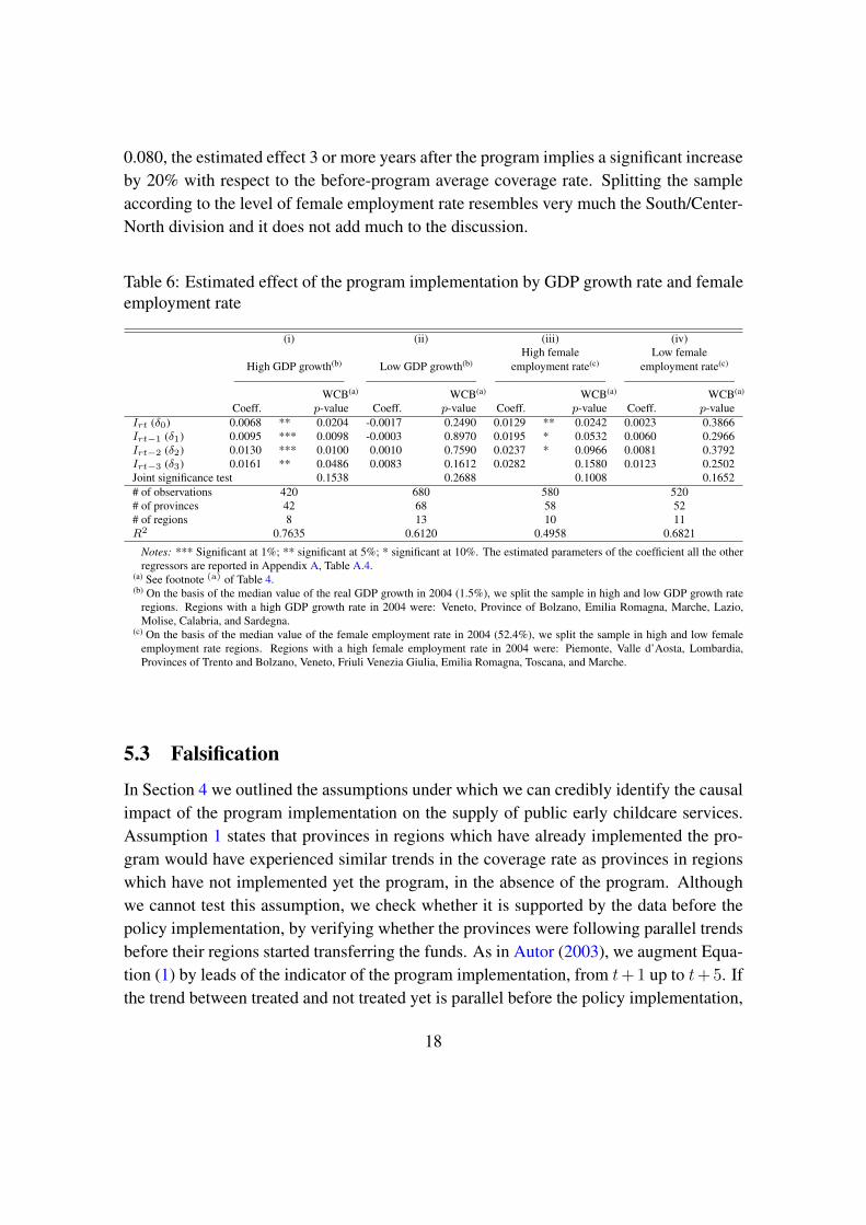
0.080, the estimated effect 3 or more years after the program implies a significant increaseby 20% with respect to the before-program average coverage rate. Splitting the sampleaccording to the level of female employment rate resembles very much the South/Center-North division and it does not add much to the discussion.

Table 6: Estimated effect of the program implementation by GDP growth rate and femaleemployment rate

(i) (ii) (iii) (iv)High female Low female

High GDP growth(b) Low GDP growth(b) employment rate(c) employment rate(c)

—————————– —————————– —————————– —————————–WCB(a) WCB(a) WCB(a) WCB(a)

Coeff. p-value Coeff. p-value Coeff. p-value Coeff. p-valueIrt (δ0) 0.0068 ** 0.0204 -0.0017 0.2490 0.0129 ** 0.0242 0.0023 0.3866Irt−1 (δ1) 0.0095 *** 0.0098 -0.0003 0.8970 0.0195 * 0.0532 0.0060 0.2966Irt−2 (δ2) 0.0130 *** 0.0100 0.0010 0.7590 0.0237 * 0.0966 0.0081 0.3792Irt−3 (δ3) 0.0161 ** 0.0486 0.0083 0.1612 0.0282 0.1580 0.0123 0.2502Joint significance test 0.1538 0.2688 0.1008 0.1652# of observations 420 680 580 520# of provinces 42 68 58 52# of regions 8 13 10 11R2 0.7635 0.6120 0.4958 0.6821

Notes: *** Significant at 1%; ** significant at 5%; * significant at 10%. The estimated parameters of the coefficient all the otherregressors are reported in Appendix A, Table A.4.

(a) See footnote (a) of Table 4.(b) On the basis of the median value of the real GDP growth in 2004 (1.5%), we split the sample in high and low GDP growth rate

regions. Regions with a high GDP growth rate in 2004 were: Veneto, Province of Bolzano, Emilia Romagna, Marche, Lazio,Molise, Calabria, and Sardegna.

(c) On the basis of the median value of the female employment rate in 2004 (52.4%), we split the sample in high and low femaleemployment rate regions. Regions with a high female employment rate in 2004 were: Piemonte, Valle d’Aosta, Lombardia,Provinces of Trento and Bolzano, Veneto, Friuli Venezia Giulia, Emilia Romagna, Toscana, and Marche.

5.3 Falsification

In Section 4 we outlined the assumptions under which we can credibly identify the causalimpact of the program implementation on the supply of public early childcare services.Assumption 1 states that provinces in regions which have already implemented the pro-gram would have experienced similar trends in the coverage rate as provinces in regionswhich have not implemented yet the program, in the absence of the program. Althoughwe cannot test this assumption, we check whether it is supported by the data before thepolicy implementation, by verifying whether the provinces were following parallel trendsbefore their regions started transferring the funds. As in Autor (2003), we augment Equa-tion (1) by leads of the indicator of the program implementation, from t+1 up to t+5. Ifthe trend between treated and not treated yet is parallel before the policy implementation,

18

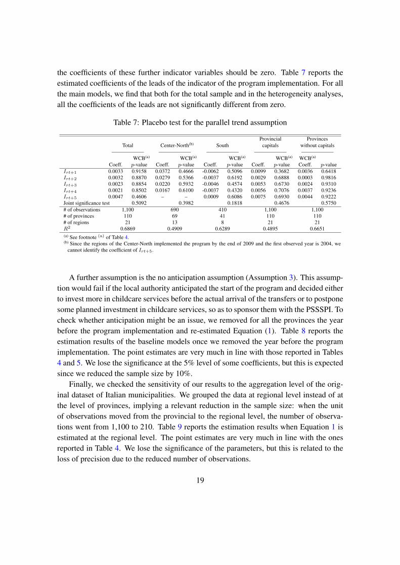
the coefficients of these further indicator variables should be zero. Table 7 reports theestimated coefficients of the leads of the indicator of the program implementation. For allthe main models, we find that both for the total sample and in the heterogeneity analyses,all the coefficients of the leads are not significantly different from zero.

Table 7: Placebo test for the parallel trend assumption

Provincial ProvincesTotal Center-North(b) South capitals without capitals

—————— —————— —————— —————— ——————WCB(a) WCB(a) WCB(a) WCB(a) WCB(a)

Coeff. p-value Coeff. p-value Coeff. p-value Coeff. p-value Coeff. p-valueIrt+1 0.0033 0.9158 0.0372 0.4666 -0.0062 0.5096 0.0099 0.3682 0.0036 0.6418Irt+2 0.0032 0.8870 0.0279 0.5366 -0.0037 0.6192 0.0029 0.6888 0.0003 0.9816Irt+3 0.0023 0.8854 0.0220 0.5932 -0.0046 0.4574 0.0053 0.6730 0.0024 0.9310Irt+4 0.0021 0.8502 0.0167 0.6100 -0.0037 0.4320 0.0056 0.7076 0.0037 0.9236Irt+5 0.0047 0.4606 – – 0.0009 0.6086 0.0075 0.6930 0.0044 0.9222Joint significance test 0.5092 0.3982 0.1818 0.4676 0.5750# of observations 1,100 690 410 1,100 1,100# of provinces 110 69 41 110 110# of regions 21 13 8 21 21R2 0.6869 0.4909 0.6289 0.4895 0.6651(a) See footnote (a) of Table 4.(b) Since the regions of the Center-North implemented the program by the end of 2009 and the first observed year is 2004, we

cannot identify the coefficient of Irt+5.

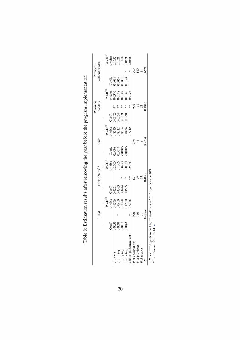
A further assumption is the no anticipation assumption (Assumption 3). This assump-tion would fail if the local authority anticipated the start of the program and decided eitherto invest more in childcare services before the actual arrival of the transfers or to postponesome planned investment in childcare services, so as to sponsor them with the PSSSPI. Tocheck whether anticipation might be an issue, we removed for all the provinces the yearbefore the program implementation and re-estimated Equation (1). Table 8 reports theestimation results of the baseline models once we removed the year before the programimplementation. The point estimates are very much in line with those reported in Tables4 and 5. We lose the significance at the 5% level of some coefficients, but this is expectedsince we reduced the sample size by 10%.

Finally, we checked the sensitivity of our results to the aggregation level of the orig-inal dataset of Italian municipalities. We grouped the data at regional level instead of atthe level of provinces, implying a relevant reduction in the sample size: when the unitof observations moved from the provincial to the regional level, the number of observa-tions went from 1,100 to 210. Table 9 reports the estimation results when Equation 1 isestimated at the regional level. The point estimates are very much in line with the onesreported in Table 4. We lose the significance of the parameters, but this is related to theloss of precision due to the reduced number of observations.

19

Tabl

e8:

Est

imat

ion

resu

ltsaf

terr

emov

ing

the

year

befo

reth

epr

ogra

mim

plem

enta

tion

Prov

inci

alPr

ovin

ces

Tota

lC

ente

r-N

orth

(b)

Sout

hca

pita

lsw

ithou

tcap

itals

——

——

——

——

——

——

——

——

——

——

——

——

——

——

——

——

——

—W

CB

(a)

WC

B(a

)W

CB

(a)

WC

B(a

)W

CB

(a)

Coe

ff.

p-v

alue

Coe

ff.

p-v

alue

Coe

ff.

p-v

alue

Coe

ff.

p-v

alue

Coe

ff.

p-v

alue

I rt

(δ0

)0.

0058

0.12

660.

0271

0.25

000.

0008

0.87

300.

0142

**0.

0346

0.00

390.

1752

I rt−

1(δ

1)

0.00

98*

0.09

000.

0373

0.13

060.

0014

0.83

120.

0264

**0.

0148

0.00

690.

1228

I rt−

2(δ

2)

0.01

190.

1098

0.04

44*

0.07

80-0

.001

50.

8554

0.02

89**

0.01

480.

0085

0.18

16I rt−

3(δ

3)

0.01

66*

0.05

300.

0505

*0.

0680

-0.0

015

0.84

540.

0350

**0.

0146

0.01

24*

0.06

28Jo

ints

igni

fican

cete

st**

0.03

36**

*0.

0076

0.77

10**

0.01

26*

0.08

68#

ofob

serv

atio

ns99

062

136

999

099

0#

ofpr

ovin

ces

110

6941

110

110

#of

regi

ons

2113

821

21R

20.

6826

0.48

250.

6234

0.48

430.

6626

Not

es:

***

Sign

ifica

ntat

1%;*

*si

gnifi

cant

at5%

;*si

gnifi

cant

at10

%.

(a)

See

foot

note

(a)

ofTa

ble

4.

20

Table 9: Baseline estimation results of the program implementation atregional level

(i) (ii) (iii)Italy Center-North South

—————————– —————————– —————————–WCB(a) WCB(a) WCB(a)

Coeff. pvalue Coeff. pvalue Coeff. pvalueIrt (δ0) 0.0024 0.5696 0.0120 * 0.0598 -0.0008 0.7226Irt−1 (δ1) 0.0050 0.5408 0.0204 * 0.0876 0.0002 0.9524Irt−2 (δ2) 0.0070 0.6074 0.0280 0.1756 -0.0013 0.8822Irt−3 (δ3) 0.0120 0.5014 0.0337 0.2512 -0.0005 0.9496Joint significance test 0.5090 0.2126 0.6512# of observations 210 130 80# of regions 21 13 8R2 0.9727 0.9514 0.9765

Notes: * Significant at 10%.(a) See footnote (a) of Table 4.

6 Conclusions

We evaluated the effectiveness of PSSSPI, a national program co-financed by regionsand started in 2007, in increasing the available slots in public early childhood education.The transfers towards public and private early childcare providers amounted to almoste1 billion. The central government designed this intervention in order to enlarge thesupply of early childcare services and to reduce the imbalances between the South andthe Center-North in the supply and use of early childcare services.

Since PSSSPI was a nationwide program, disentangling the impact of the time trendfrom the true effect of the program is not trivial. However, the transfers from the centralgovernment to the regional authority did not take place at the same moment in each region.Regions had indeed to pass a set of acts to receive the transfers from the central govern-ment to update their legislation about the different types of early childcare services and todesign the executive authorizing procedures for transferring grants to the final childcareservice providers. We took advantage of the different timing of transfers across regionsand, by the DiD technique, we estimated the causal impact of PSSSPI on the availableslots in public early childhood education. The empirical analysis is based on a dataset atthe municipal level collected by the Italian Department of Territorial and Internal Affairsover the years 2004-2013. We aggregated the data at the level of the 110 Italian provinceswhich are observed for 10 years.

We found that PSSSPI was only partially successful. Whilst on average in Italy three(or more) years after the program intervention the available slots in public early childhoodeducation increased by 18.1% with respect to the pre-intervention average, the program

21

impact was not homogeneous across regions. We showed indeed that the program effec-tiveness was nil in the Southern regions and quite strong in the Center-North where, threeor more years after the policy implementation, the increase in the coverage rate amountedto more than 30% and characterized both provincial capitals and the rest of the territory.Hence, the program failed in reducing regional differences in the supply of early childcareservices, at least the public ones. The reasons of this failure are not in question in thispaper, but they should be investigated in order to design policy interventions that might befully effective in reducing regional disparities in the availability of public early childcareservices and, thereby, in the maternal employment rates.

ReferencesAkgunduz, Y. and J. Plantenga (2018). Child care prices and maternal employment: A meta-analysis.

Journal of Economics Surveys 32(1), 118–133.

Autor, D. H. (2003). Outsourcing at will: The contribution of unjust dismissal doctrine to the growth ofemployment outsourcing. Journal of Labor Economics 21(1), 1–42.

Bandiera, O., A. Prat, and T. Valletti (2009). Active and passive waste in government spending: Evidencefrom a policy experiment. American Economic Review 99(4), 1278–1308.

Barone, G. and G. Narciso (2013). The effect of organized crime on public funds. Temi di discussione dellaBanda d’Italia, Working Paper No. 916.

Bettendorf, L., E. Jongen, and P. Muller (2015). Childcare subsidies and labour supply-evidence from aDutch reform. Labour Economics 36(C), 112–123.

Blau, D. (2003). Child care subsidy programs. In R. Moffit (Ed.), Means Tested Social Programs, pp.443–516. University of Chicago Press.

Blau, D. and J. Currie (2006). Pre-school, day care, and after-school care: Who’s minding the kids? InE. Hanushek and F. Welch (Eds.), Handbook of the Economics of Education, Volume 2, Chapter 20, pp.1163–1278. Elsevier.

Blau, D. and P. Robins (1988). Child care costs and family labor supply. Review of Economics andStatistics 70(3), 374–381.

Bratti, M., E. Del Bono, and D. Vuri (2005). New mothers’ labour force participation in Italy: The role ofjob characteristics. Labour 19(s1), 79–121.

Brilli, Y., D. Del Boca, and C. Pronzato (2016). Does child care availability play a role in maternal employ-ment and children’s development? Evidence from Italy. Review of Economics of the Household 14(1),27–51.

22

Brollo, F., T. Nannicini, R. Perotti, and G. Tabellini (2013). The political resource curse. American Eco-nomic Review 103(5), 1759–1796.

Cameron, A. C., J. B. Gelbach, and D. L. Miller (2008). Bootstrap-based improvements for inference withclustered errors. Review of Economics and Statistics 90(3), 414–427.

Cameron, A. C. and D. L. Miller (2015). A practitioner’s guide to cluster-robust inference. Journal ofHuman Resources 50(2), 371–372.

Carozzi, F. and L. Repetto (2016). Sending the pork home: Birth town bias in transfers to Italian munici-palities. Journal of Public Economics 134(C), 42–52.

CEU (2000). Council of the European Union. Presidency Conclusions. Lisbon European Council, 23rd and24th March. Brussels.

CEU (2002). Council of the European Union. Barcelona European Council 15-16 March. Presidency con-clusions. http://aei.pitt.edu/43345/1/Barcelona_2002_1.pdf.

De Angelis, I., G. de Blasio, and L. Rizzica (2018). On the unintended effects of public transfers: Evidencefrom EU funding to Southern Italy. Temi di discussione della Banda d’Italia, Working Paper No. 1180.

Del Boca, D. (2002). The effect of child care and part time opportunities on participation and fertilitydecisions in Italy. Journal of Population Economics 15(3), 549–573.

Del Boca, D., M. Locatelli, and D. Vuri (2005). Child-care choices by working mothers: The case of Italy.Review of Economics of the Household 3(4), 453–477.

Del Boca, D., S. Pasqua, and C. Pronzato (2009). Motherhood and market work decisions in institutionalcontext: A European perspective. Oxford Economic Papers 61(Suppl. 1), i147–i171.

Del Boca, D. and R. M. Sauer (2009). Lifecycle employment and fertility across institutional enviroments.European Economic Review 53(3), 274–292.

Del Boca, D. and D. Vuri (2007). The mismatch between employment and child care in Italy: The impactof rationing. Journal of Population Economics 20(4), 805–832.

European Commission (2010). Europe 2020. A strategy for smart, sustainable and inclusive growth.Communication from the Commission. COM (2010) 2020 final, 3 March 2010. Brussels. http://eur-lex.europa.eu/LexUriServ/LexUriServ.do?uri=COM:2010:2020:FIN:EN:PDF.

Figari, F. and E. Narazani (2017). Female labour supply and childcare in Italy. JRC Working Papers onTaxation and Structural Reforms N.02/2017, European Commission, Joint Research Centre, Seville.

Givord, P. and C. Marbot (2015). Does the cost of child care affect female labor market participation? Anevaluation of a French reform of childcare subsidies. Labour Economics 36(C), 99–111.

Havnes, T. and M. Mogstad (2011). Money for nothing? Universal child care and maternal employment.Journal of Public Economics 95(11), 1455–1465.

23

ISTAT (2016). L’offerta comunale di asili nido e altri servizi socio-educativi per la prima infanzia. Annoscolastico 2013/2014. Statistiche Report. Istituto nazionale di statistica, Rome.

Istituto degli Innocenti (2009, December). Monitoraggio del Piano di sviluppo dei servizi socio-educativiper prima infanzia. Centro nazionale di documentazione e analisi per l’infanzia e l’adolescenza.Litografia IP di Firenze.

Istituto degli Innocenti (2014). Monitoraggio del Piano di sviluppo dei servizi socio-educativi per primainfanzia. Centro nazionale di documentazione e analisi per l’infanzia e l’adolescenza. Litografia IP diFirenze.

Liang, K.-Y. and S. L. Zeger (1986). Longitudinal data analysis using generalized linear models.Biometrika 73(1), 13–22.

Lundin, D., E. Mörk, and B. Öckert (2008). How far can reduced childcare prices push female laboursupply? Labour Economics 15(4), 647–659.

Milio, S. (2007). Can administrative capacity explain differences in regional performances? Evidence fromstructural funds implementation in Southern Italy. Regional Studies 41(4), 429–442.

Ribar, D. (1995). A structural model of child care and the labor supply of married women. Journal of LaborEconomics 13(3), 558–597.

Soncin, S. (2013). Gli asili nido. In M. Stefani (Ed.), Le normative e le politiche regionali per la parteci-pazione delle donne al mercato del lavoro. Questioni di Economia e Finanza (Occasional papers) No.189, Chapter 9, pp. 64–73. Bank of Italy.

Valdelanoote, D., P. Vanleenhove, A. Decoster, J. Ghysels, and G. Verbist (2015). Maternal employment:The impact of the triple rationing in childcare in Flanders. Review of Economics of the Households 13(3),685–707.

Webb, M. D. (2014). Reworking wild bootstrap based inference for clustered errors. Queen’s EconomicsDepartment Working Paper No. 1315, Kingston, Canada.

Wrohlich, K. (2004). Child care costs and mothers’ labor supply: An empirical analysis for Germany.Discussion Paper 412 DIW Berlin, German Institute for Economic Research.

24

Appendix

A Full set of estimation results

Table A.1: Full set of estimation results of the results reported in Table 4

(i) (ii) (iii)Italy Center-North South

—————————– —————————– —————————–Coeff. Std. Err.(a) Coeff. Std. Err.(a) Coeff. Std. Err.(a)

Program implementation impactIrt (δ0) 0.0043 * 0.0022 0.0140 *** 0.0018 0.0011 0.0023Irt−1 (δ1) 0.0075 ** 0.0030 0.0229 *** 0.0039 0.0019 0.0040Irt−2 (δ2) 0.0096 ** 0.0040 0.0289 *** 0.0053 -0.0008 0.0048Irt−3 (δ3) 0.0142 *** 0.0046 0.0338 *** 0.0071 -0.0006 0.0050

Region - Reference: Piemonte (Campania in model iii)Valle d’Aosta 0.0051 0.0032 -0.0031 0.0053 – –Lombardia -0.0304 *** 0.0003 -0.0311 *** 0.0005 – –Province of Trento 0.0198 *** 0.0028 0.0107 ** 0.0049 – –Veneto -0.0460 *** 0.0017 -0.0437 *** 0.0026 – –Fiuli Venezia Giulia -0.0024 *** 0.0007 -0.0007 0.0011 – –Liguria 0.0058 *** 0.0019 0.0109 *** 0.0033 – –Emilia Romagna 0.0700 *** 0.0043 0.0570 *** 0.0074 – –Toscana 0.0367 *** 0.0007 0.0386 *** 0.0012 – –Umbria -0.0058 *** 0.0020 -0.0007 0.0034 – –Marche -0.0002 0.0011 0.0026 0.0018 – –Lazio -0.0284 *** 0.0059 -0.0150 0.0097 – –Abruzzo -0.0345 *** 0.0093 – – 0.0342 *** 0.0059Molise -0.0634 *** 0.0139 – – 0.0044 0.0041Campania -0.0547 ** 0.0237 – – – –Puglia -0.0482 ** 0.0220 – – 0.0094 *** 0.0007Basilicata -0.0324 * 0.0174 – – 0.0308 *** 0.0026Calabria -0.0633 *** 0.0209 – – -0.0047 *** 0.0012Sicilia -0.0173 0.0227 – – 0.0398 *** 0.0006Sardegna -0.0288 ** 0.0132 – – 0.0380 *** 0.0043Province of Bolzano -0.0633 *** 0.0028 -0.0685 *** 0.0049 – –

Year - Reference: 20042005 0.0019 * 0.0010 0.0018 0.0019 0.0008 0.00112006 0.0015 0.0015 -0.0008 0.0027 0.0011 0.00182007 0.0029 * 0.0016 -0.0039 0.0035 0.0029 ** 0.00112008 0.0002 0.0029 -0.0170 *** 0.0049 0.0027 0.00172009 0.0005 0.0037 -0.0180 *** 0.0055 0.0029 0.00292010 -0.0010 0.0040 -0.0210 *** 0.0063 0.0030 0.00382011 -0.0033 0.0049 -0.0237 *** 0.0078 0.0039 0.00462012 -0.0072 0.0060 -0.0283 *** 0.0096 0.0038 0.00512013 -0.0083 0.0059 -0.0288 *** 0.0093 0.0029 0.0051

Regional female employment rate 0.0015 * 0.0008 0.0037 *** 0.0014 0.0008 * 0.0003Regional real GDP growth rate 0.0000 0.0002 0.0000 0.0003 0.0000 0.0001Constant 0.0986 *** 0.0055 0.0851 *** 0.0086 0.0283 *** 0.0068# of observations 1,100 690 410# of provinces 110 69 41# of regions 21 13 8R2 0.6868 0.4902 0.6280

Notes: *** Significant at 1%; ** significant at 5%; * significant at 10%.(a) CRVE standard errors.

25

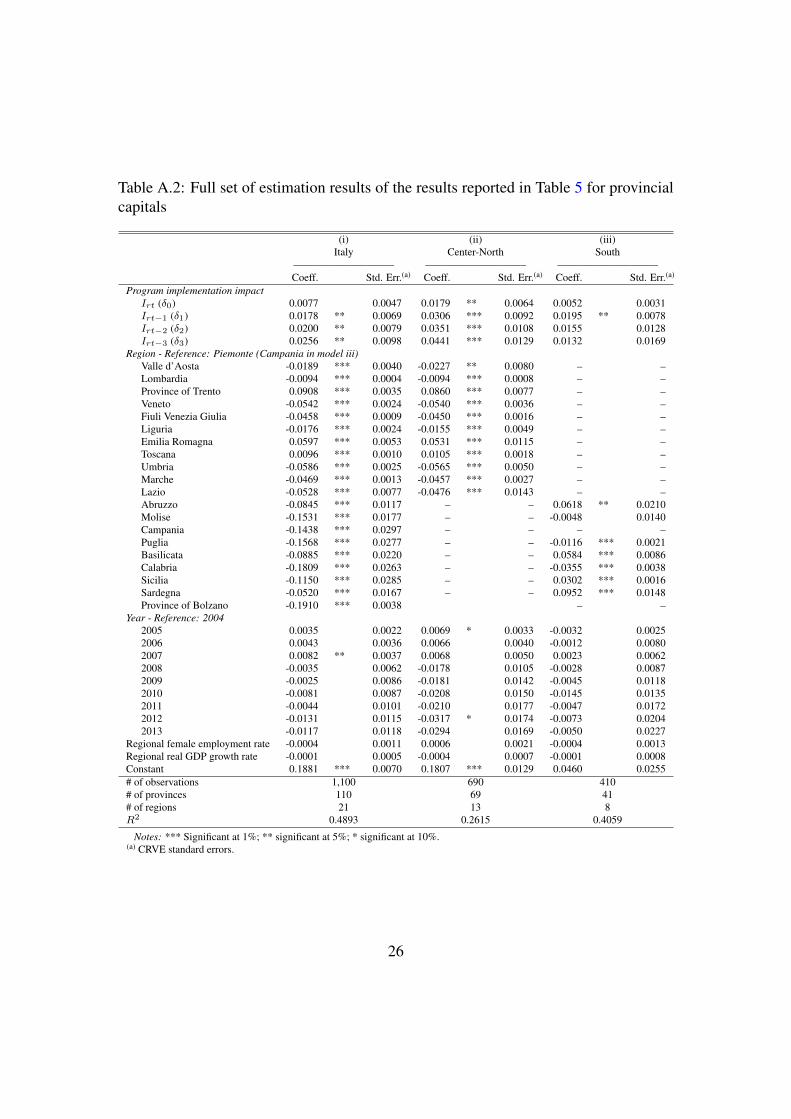
Table A.2: Full set of estimation results of the results reported in Table 5 for provincialcapitals

(i) (ii) (iii)Italy Center-North South

—————————– —————————– —————————–Coeff. Std. Err.(a) Coeff. Std. Err.(a) Coeff. Std. Err.(a)

Program implementation impactIrt (δ0) 0.0077 0.0047 0.0179 ** 0.0064 0.0052 0.0031Irt−1 (δ1) 0.0178 ** 0.0069 0.0306 *** 0.0092 0.0195 ** 0.0078Irt−2 (δ2) 0.0200 ** 0.0079 0.0351 *** 0.0108 0.0155 0.0128Irt−3 (δ3) 0.0256 ** 0.0098 0.0441 *** 0.0129 0.0132 0.0169

Region - Reference: Piemonte (Campania in model iii)Valle d’Aosta -0.0189 *** 0.0040 -0.0227 ** 0.0080 – –Lombardia -0.0094 *** 0.0004 -0.0094 *** 0.0008 – –Province of Trento 0.0908 *** 0.0035 0.0860 *** 0.0077 – –Veneto -0.0542 *** 0.0024 -0.0540 *** 0.0036 – –Fiuli Venezia Giulia -0.0458 *** 0.0009 -0.0450 *** 0.0016 – –Liguria -0.0176 *** 0.0024 -0.0155 *** 0.0049 – –Emilia Romagna 0.0597 *** 0.0053 0.0531 *** 0.0115 – –Toscana 0.0096 *** 0.0010 0.0105 *** 0.0018 – –Umbria -0.0586 *** 0.0025 -0.0565 *** 0.0050 – –Marche -0.0469 *** 0.0013 -0.0457 *** 0.0027 – –Lazio -0.0528 *** 0.0077 -0.0476 *** 0.0143 – –Abruzzo -0.0845 *** 0.0117 – – 0.0618 ** 0.0210Molise -0.1531 *** 0.0177 – – -0.0048 0.0140Campania -0.1438 *** 0.0297 – – – –Puglia -0.1568 *** 0.0277 – – -0.0116 *** 0.0021Basilicata -0.0885 *** 0.0220 – – 0.0584 *** 0.0086Calabria -0.1809 *** 0.0263 – – -0.0355 *** 0.0038Sicilia -0.1150 *** 0.0285 – – 0.0302 *** 0.0016Sardegna -0.0520 *** 0.0167 – – 0.0952 *** 0.0148Province of Bolzano -0.1910 *** 0.0038 – –

Year - Reference: 20042005 0.0035 0.0022 0.0069 * 0.0033 -0.0032 0.00252006 0.0043 0.0036 0.0066 0.0040 -0.0012 0.00802007 0.0082 ** 0.0037 0.0068 0.0050 0.0023 0.00622008 -0.0035 0.0062 -0.0178 0.0105 -0.0028 0.00872009 -0.0025 0.0086 -0.0181 0.0142 -0.0045 0.01182010 -0.0081 0.0087 -0.0208 0.0150 -0.0145 0.01352011 -0.0044 0.0101 -0.0210 0.0177 -0.0047 0.01722012 -0.0131 0.0115 -0.0317 * 0.0174 -0.0073 0.02042013 -0.0117 0.0118 -0.0294 0.0169 -0.0050 0.0227

Regional female employment rate -0.0004 0.0011 0.0006 0.0021 -0.0004 0.0013Regional real GDP growth rate -0.0001 0.0005 -0.0004 0.0007 -0.0001 0.0008Constant 0.1881 *** 0.0070 0.1807 *** 0.0129 0.0460 0.0255# of observations 1,100 690 410# of provinces 110 69 41# of regions 21 13 8R2 0.4893 0.2615 0.4059

Notes: *** Significant at 1%; ** significant at 5%; * significant at 10%.(a) CRVE standard errors.

26

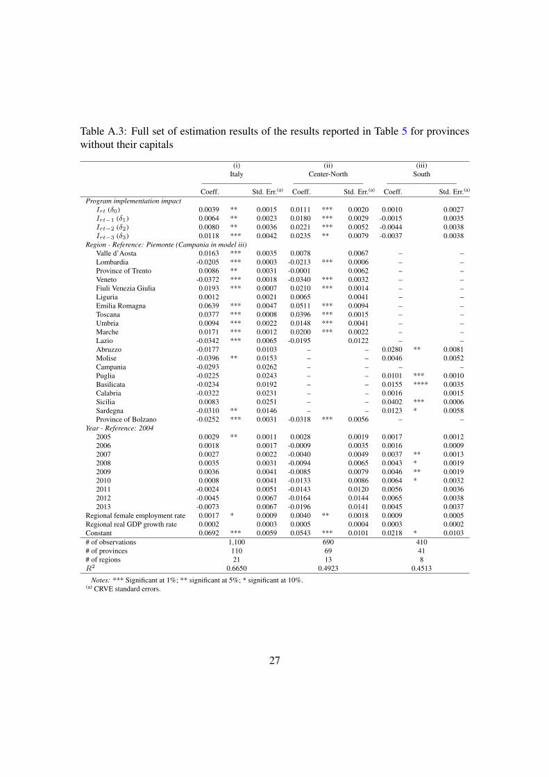
Table A.3: Full set of estimation results of the results reported in Table 5 for provinceswithout their capitals

(i) (ii) (iii)Italy Center-North South

—————————– —————————– —————————–Coeff. Std. Err.(a) Coeff. Std. Err.(a) Coeff. Std. Err.(a)

Program implementation impactIrt (δ0) 0.0039 ** 0.0015 0.0111 *** 0.0020 0.0010 0.0027Irt−1 (δ1) 0.0064 ** 0.0023 0.0180 *** 0.0029 -0.0015 0.0035Irt−2 (δ2) 0.0080 ** 0.0036 0.0221 *** 0.0052 -0.0044 0.0038Irt−3 (δ3) 0.0118 *** 0.0042 0.0235 ** 0.0079 -0.0037 0.0038

Region - Reference: Piemonte (Campania in model iii)Valle d’Aosta 0.0163 *** 0.0035 0.0078 0.0067 – –Lombardia -0.0205 *** 0.0003 -0.0213 *** 0.0006 – –Province of Trento 0.0086 ** 0.0031 -0.0001 0.0062 – –Veneto -0.0372 *** 0.0018 -0.0340 *** 0.0032 – –Fiuli Venezia Giulia 0.0193 *** 0.0007 0.0210 *** 0.0014 – –Liguria 0.0012 0.0021 0.0065 0.0041 – –Emilia Romagna 0.0639 *** 0.0047 0.0511 *** 0.0094 – –Toscana 0.0377 *** 0.0008 0.0396 *** 0.0015 – –Umbria 0.0094 *** 0.0022 0.0148 *** 0.0041 – –Marche 0.0171 *** 0.0012 0.0200 *** 0.0022 – –Lazio -0.0342 *** 0.0065 -0.0195 0.0122 – –Abruzzo -0.0177 0.0103 – – 0.0280 ** 0.0081Molise -0.0396 ** 0.0153 – – 0.0046 0.0052Campania -0.0293 0.0262 – – – –Puglia -0.0225 0.0243 – – 0.0101 *** 0.0010Basilicata -0.0234 0.0192 – – 0.0155 **** 0.0035Calabria -0.0322 0.0231 – – 0.0016 0.0015Sicilia 0.0083 0.0251 – – 0.0402 *** 0.0006Sardegna -0.0310 ** 0.0146 – – 0.0123 * 0.0058Province of Bolzano -0.0252 *** 0.0031 -0.0318 *** 0.0056 – –

Year - Reference: 20042005 0.0029 ** 0.0011 0.0028 0.0019 0.0017 0.00122006 0.0018 0.0017 -0.0009 0.0035 0.0016 0.00092007 0.0027 0.0022 -0.0040 0.0049 0.0037 ** 0.00132008 0.0035 0.0031 -0.0094 0.0065 0.0043 * 0.00192009 0.0036 0.0041 -0.0085 0.0079 0.0046 ** 0.00192010 0.0008 0.0041 -0.0133 0.0086 0.0064 * 0.00322011 -0.0024 0.0051 -0.0143 0.0120 0.0056 0.00362012 -0.0045 0.0067 -0.0164 0.0144 0.0065 0.00382013 -0.0073 0.0067 -0.0196 0.0141 0.0045 0.0037

Regional female employment rate 0.0017 * 0.0009 0.0040 ** 0.0018 0.0009 0.0005Regional real GDP growth rate 0.0002 0.0003 0.0005 0.0004 0.0003 0.0002Constant 0.0692 *** 0.0059 0.0543 *** 0.0101 0.0218 * 0.0103# of observations 1,100 690 410# of provinces 110 69 41# of regions 21 13 8R2 0.6650 0.4923 0.4513

Notes: *** Significant at 1%; ** significant at 5%; * significant at 10%.(a) CRVE standard errors.

27

Table A.4: Full set of estimation results of the results reported in Table 6

(i) (ii) (iii) (iv)High female Low female

High GDP Low GDP employment employmentgrowth(b) growth(b) rate(c) rate(c)

—————————– —————————– —————————– —————————–Coeff. SE(a) Coeff. SE(a) Coeff. SE(a) Coeff. SE(a)

Program implementation impactIrt (δ0) 0.0068 ** 0.0022 -0.0017 0.0014 0.0129 *** 0.0020 0.0023 0.0019Irt−1 (δ1) 0.0095 ** 0.0029 -0.0003 0.0023 0.0195 *** 0.0043 0.0060 0.0034Irt−2 (δ2) 0.0130 ** 0.0040 0.0010 0.0037 0.0237 *** 0.0059 0.0081 0.0053Irt−3 (δ3) 0.0161 ** 0.0057 0.0083 0.0050 0.0282 *** 0.0082 0.0123 * 0.0064

Region - Reference: Piemonte (Emilia Romagna in model i and Campania in model iv)Valle d’Aosta – – 0.0035 0.0028 -0.0055 0.0068 – –Lombardia – – -0.0304 *** 0.0003 -0.0313 *** 0.0006 – –Province of Trento – – 0.0193 *** 0.0022 0.0091 0.0061 – –Veneto -0.1130 *** 0.0105 – – -0.0419 *** 0.0035 – –Fiuli Venezia Giulia – – -0.0020 *** 0.0006 -0.0002 0.0014 – –Liguria – – 0.0067 *** 0.0017 – – 0.0849 *** 0.0156Emilia Romagna – – – – 0.0542 *** 0.0094 – –Toscana – – 0.0372 *** 0.0006 0.0391 *** 0.0015 – –Umbria – – -0.0050 ** 0.0017 – – 0.0732 *** 0.0156Marche -0.0670 *** 0.0096 – – 0.0034 0.0023 – –Lazio -0.0935 *** 0.0181 – – – – 0.0466 *** 0.0126Abruzzo – – -0.0302 *** 0.0079 – – 0.0363 *** 0.0103Molise -0.1237 *** 0.0325 – – – – 0.0026 0.0070Campania – – -0.0442 ** 0.0202 – – – –Puglia – – -0.0377 * 0.0189 – – 0.0086 *** 0.0012Basilicata – – -0.0236 0.0151 – – 0.0297 *** 0.0045Calabria -0.1205 ** 0.0449 – – – – -0.0053 ** 0.0020Sicilia – – -0.0065 0.0195 – – 0.0388 *** 0.0008Sardegna -0.0899 ** 0.0312 – – – – 0.0379 *** 0.0074Province of Bolzano -0.1330 *** 0.0030 – – -0.0714 *** 0.0063 – –

Year - Reference: 20042005 0.0049 ** 0.0015 0.0009 0.0014 0.0010 0.0022 0.0018 0.00162006 0.0048 ** 0.0016 -0.0008 0.0015 -0.0021 0.0035 0.0021 0.00152007 0.0055 ** 0.0020 0.0001 0.0018 -0.0049 0.0040 0.0044 *** 0.00132008 0.0032 0.0040 0.0007 0.0017 -0.0172 *** 0.0050 0.0037 * 0.00192009 0.0041 0.0055 0.0036 0.0027 -0.0154 ** 0.0059 0.0025 0.00272010 -0.0024 0.0052 0.0068 * 0.0031 -0.0175 ** 0.0069 0.0007 0.00332011 -0.0054 0.0062 0.0032 0.0052 -0.0196 * 0.0089 -0.0026 0.00502012 -0.0085 0.0096 -0.0016 0.0064 -0.0246 * 0.0110 -0.0056 0.00612013 -0.0058 0.0101 -0.0046 0.0061 -0.0260 ** 0.0111 -0.0062 0.0053

Regional female emp. rate 0.0019 0.0015 0.0019 ** 0.0007 0.0043 ** 0.0018 0.0006 0.0006Regional GDP growth rate 0.0006 0.0006 -0.0003 0.0003 0.0001 0.0004 -0.0002 0.0002Constant 0.1605 *** 0.0180 0.0973 *** 0.0050 0.0816 *** 0.0112 0.0238 * 0.0129# of observations 420 680 580 520# of provinces 42 68 58 52# of regions 8 13 10 11R2 0.7635 0.6120 0.4958 0.6821

Notes: *** Significant at 1%; ** significant at 5%; * significant at 10%.(a) CRVE standard errors.(b) On the basis of the median value of the real GDP growth in 2004 (1.5%), we split the sample in high and low GDP growth rate regions. Regions with a high

GDP growth rate in 2004 were: Veneto, Province of Bolzano, Emilia Romagna, Marche, Lazio, Molise, Calabria, and Sardegna.(c) On the basis of the median value of the female employment rate in 2004 (52.4%), we split the sample in high and low female employment rate regions. Regions

with a high female employment rate in 2004 were: Piemonte, Valle d’Aosta, Lombardia, Provinces of Trento and Bolzano, Veneto, Friuli Venezia Giulia, EmiliaRomagna, Toscana, and Marche.

28