ESI The Erwin Schrodinger International Boltzmanngasse 9Institute for Mathematical Physics A-1090 Wien, Austria

On Spectral Problems Related to a Time DependentModel in Superconductivity with Electric Current

B. Helffer

Vienna, Preprint ESI 2192 (2009) November 10, 2009

Supported by the Austrian Federal Ministry of Education, Science and CultureAvailable online at http://www.esi.ac.at

On spectral problems related to a time

dependent model in superconductivity with

electric current.

B. Helffer (Univ Paris-Sud and CNRS)∗

Abstract

This lecture is mainly inspired by a paper of Y. Almog appearinglast year at Siam J. Math. Anal. Our goal here is first to discuss indetail the simplest models which we think are enlightning for under-standing the role of the pseudospectra in this question and secondlyto present proofs which will have some general character and will forexample apply in a more physical model, for which we have obtainedrecently results together with Y. Almog and X. Pan.

1 Introduction

We would like to understand the following problem coming from supercon-ductivity. We consider a superconductor placed in an applied magnetic fieldand submitted to an electric current through the sample. It is usually saidthat if the applied magnetic field is sufficiently high, or if the electric currentis strong, then the sample is in a normal state. We are interested in analyz-ing the joint effect of the applied field and the current on the stability of thenormal state. As described for example in our recent book with S. Fournais[FoHel], this kind of question, without magnetic fields, can be treated by us-ing fine results on the spectral theory of Schrodinger operator with magneticfield starting with the analysis of the case with constant magnetic field in the

∗The author was also visiting the Erwin Schrodinger Institute in Vienna when writingthis paper.

1

whole space and in the half-space. So we would like to start an analogousanalysis when an electric current is considered.

This lecture is mainly inspired by a paper of Y. Almog [Alm2]. Our maingoal here is to discuss in details the simplest models which we think areenlightning for understanding the role of the pseudospectra in this question.In the second part, we will present proofs which have some general characterand for example apply in a more physical model, involving for example thenon self-adjoint operator −∂2

x − (∂y − ix2

2)2 + i y on R

2x,y, ,for which we have

obtained recently results together with Y. Almog and X. Pan [AHP].After a presentation in the next section of the general problems and of

our main results, we will come back to Almog’s analysis and will start froma fine “pseudo-spectral” analysis for the complex Airy operator on −∂2

x + i xon the line or on R

+ and make a survey of what is known.We hope also that this will illustrate some aspects discussed in the lectures

of J. Sjostrand at this conference. They are also related to recent results ofGallagher-Gallay-Nier [GGN] and to results on the Fokker-Planck equationobtained by Helffer, Herau, Nier ([HelNi] and references therein) or Villani[Vil].

AcknowledgementsDuring the preparation of these notes we have benefitted, in addition to thecollaboration with Y. Almog and X. Pan, of discussions with many colleaguesincluding W. Bordeaux-Montrieux, B. Davies, P. Gerard, C. Han, F. Herau,J. Martinet, F. Nier and J. Sjostrand. In addition, W. Bordeaux-Montrieuxand K. Pravda-Starov provide us also with numerical computations whichwere sometimes confirming and sometimes predicting interesting properties.

2 The model in superconductivity

2.1 General context

Coming back to the physical motivation, let us consider a two-dimensionalsuperconducting sample capturing the entire xy plane. We can assume alsothat a magnetic field of magnitude He is applied perpendicularly to thesample. Denote the Ginzburg-Landau parameter of the superconductor byκ (κ > 0) and the normal conductivity of the sample by σ.

2

The physical problem is posed in a domain Ω with specific boundaryconditions. We will only analyze here limiting situations where the domainpossibly after a blowing argument becomes the whole space (or the half-space). We will mainly work in dimension 2 for simplification.

Then the time-dependent Ginzburg-Landau system (also known as theGorkov-Eliashberg equations) is in ]0, T [×Ω :

∂tψ + iκΦψ = −∆κAψ + κ2(1 − |ψ|2)ψ ,κ2 curl 2A + σ(∂tA + ∇Φ) = κIm (ψ∇κAψ) + κ2 curl He ,

(2.1)

where ψ is the order parameter, A the magnetic potential, Φ the electricpotential, ∇κA = ∇ + iκA and −∆κA is the magnetic Laplacian associatedwith magnetic potential κA.In addition (ψ,A,Φ) satisfies an initial condition at t = 0.

In order to solve this equation, one should also define a gauge (Coulomb,Lorentz,...). The orbit of (ψ,A,Φ) by the gauge group is

(exp iκq ψ,A + ∇q,Φ − ∂tq) | q ∈ Q ,

where Q is a suitable space of regular functions of (x, t). We refer to[BJP] (Paragraph B in the introduction) for a discussion of this point. Wewill choose the Coulomb gauge which reads that we can add the conditiondiv A = 0 for any t. Another possibility could be to take div A + σΦ = 0.

A solution (ψ,A,Φ) is called a normal state solution if ψ = 0.

2.2 Stationary normal solutions

From (2.1), we see that if (0,A,Φ) is a time-independent normal statesolution, then (A,Φ) satisfies the equality

κ2 curl 2A + σ∇Φ = κ2 curl He , div A = 0 in Ω . (2.2)

(Note that if one identifies He to a function h, then curl He = (−∂yh , ∂xh).)Interpreting these equations as the Cauchy-Riemann equations, this can berewritten as the property that

κ2( curl A −He) + i σΦ ,

is an holomorphic function in Ω. In particular, if σ 6= 0, Φ and curl A−He

are harmonic.

3

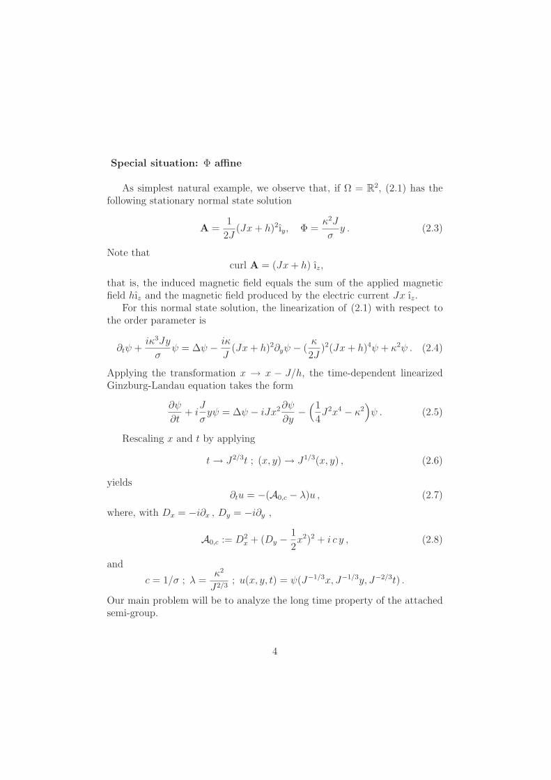
Special situation: Φ affine

As simplest natural example, we observe that, if Ω = R2, (2.1) has the

following stationary normal state solution

A =1

2J(Jx+ h)2 ıy, Φ =

κ2J

σy . (2.3)

Note thatcurl A = (Jx+ h) ız,

that is, the induced magnetic field equals the sum of the applied magneticfield hız and the magnetic field produced by the electric current Jx ız.

For this normal state solution, the linearization of (2.1) with respect tothe order parameter is

∂tψ +iκ3Jy

σψ = ∆ψ − iκ

J(Jx+ h)2∂yψ − (

κ

2J)2(Jx+ h)4ψ + κ2ψ . (2.4)

Applying the transformation x → x − J/h, the time-dependent linearizedGinzburg-Landau equation takes the form

∂ψ

∂t+ i

J

σyψ = ∆ψ − iJx2∂ψ

∂y−

(1

4J2x4 − κ2

)ψ . (2.5)

Rescaling x and t by applying

t→ J2/3t ; (x, y) → J1/3(x, y) , (2.6)

yields∂tu = −(A0,c − λ)u , (2.7)

where, with Dx = −i∂x , Dy = −i∂y ,

A0,c := D2x + (Dy −

1

2x2)2 + i c y , (2.8)

and

c = 1/σ ; λ =κ2

J2/3; u(x, y, t) = ψ(J−1/3x, J−1/3y, J−2/3t) .

Our main problem will be to analyze the long time property of the attachedsemi-group.

4

We now apply the transformation

u→ u eicyt

to obtain

∂tu = −(D2

xu+ (Dy −1

2x2 − ct)2u− λu

). (2.9)

Note that considering the partial Fourier transform, we obtain

∂tu = −D2xu−

[(1

2x2 + (ct− ω)

)2

− λ

]u . (2.10)

This can be rewritten as the analysis of a family (depending on ω ∈ R)of time-dependent problems on the line

∂tu = −Lβ(t,ω)u+ λu , (2.11)

with Lβ being the well-known anharmonic oscillator (or Montgomery opera-tor) :

Lβ = D2x + (

1

2x2 + β)2 , (2.12)

andβ(t, ω) = ct− ω .

Note that in this point of view, we can after a change of time look at thefamily of problems

∂τv(x, τ) = −(Lcτv)(x, τ) + λv(x, τ) , (2.13)

the initial condition at t = 0 becoming at τ = −ωc.

2.3 Recent results by Almog-Helffer-Pan [AHP]

The main point concerning the previously defined operator is to obtain resultswhich are quite close to the Airy operator on the line.

Theorem 2.1If c 6= 0, A = A0,c has compact resolvent, empty spectrum, and there existsC > 0 such that

‖ exp(−tA)‖ ≤ exp(−2

√2c

3t3/2 + Ct3/4

), (2.14)

5

for any t ≥ 1 and

‖(A− λ)−1‖ ≤ exp( 1

6cReλ3 + C Reλ3/2

), (2.15)

for all λ such that Reλ ≥ 1.

Here we can no longer use the explicit properties of the Airy function but asemi-classical analysis of the operator Lβ as |β| → +∞ plays an importantrole. We refer to [AHP] for details.

3 A simplified model : no magnetic field

We assume, following Almog, that a current of constant magnitude J is beingflown through the sample in the x axis direction, and h = 0. Then (2.1) has(in some asymptotic regime) the following stationary normal state solution

A = 0 , Φ = Jx . (3.1)

For this normal state solution, the linearization of (2.1) gives

∂tψ + iJxψ = ∆x,yψ + ψ , (3.2)

whose analysis is (see ahead) strongly related to the Airy equation.

3.1 The complex Airy operator in R

This operator can be defined as the closed extension A of the differentialoperator on C∞

0 (R) A+0 := D2

x + i x . We observe that A = (A−0 )∗ with

A−0 := D2

x − i x and that its domain is

D(A) = u ∈ H2(R) , x u ∈ L2(R) .

In particular A has compact resolvent.It is also easy to see that

Re 〈Au |u〉 ≥ 0 . (3.3)

Hence −A is the generator of a semi-group St of contraction,

St = exp−tA . (3.4)

6

Hence all the results of this theory can be applied.In particular, we have, for Reλ < 0

||(A− λ)−1|| ≤ 1

|Reλ| . (3.5)

One can also show that the operator is maximally accretive.A very special property of this operator is that, for any a ∈ R,

TaA = (A− ia)Ta , (3.6)

where Ta is the translation operator (Tau)(x) = u(x− a) .As immediate consequence, we obtain that the spectrum is empty and thatthe resolvent of A, which is defined for any λ ∈ C satisfies

||(A− λ)−1|| = ||(A− Reλ)−1|| . (3.7)

One can also look at the semi-classical question, i.e. look

Ah = h2D2x + i x , (3.8)

and observe that it is the toy model for some results of Dencker-Sjostrand-Zworski [DSZ]. Of course in such an homogeneous situation one can go fromone point of view to the other but it is sometimes good to look at what eachtheory gives on this very particular model. This for example interacts withthe first part of the lectures by J. Sjostrand [Sjo2].

The most interesting property is the control of the resolvent for Reλ ≥ 0.

Proposition 3.1There exist two positive constants C1 and C2, such that

C1 |Reλ|− 1

4 exp4

3Reλ

3

2 ≤ ||(A− λ)−1|| ≤ C2 |Reλ|− 1

4 exp4

3Reλ

3

2 , (3.9)

(see Martinet [Mart] for this fine version). Note that W. Bordeaux-Montrieuxand J. Sjostrand1 have obtained a better result.

The proof of the (rather standard) upper bound is based on the directanalysis of the semi-group in the Fourier representation. We note indeed that

F(D2x + i x)F−1 = ξ2 +

d

dξ. (3.10)

1Personnal communication

7

Then we have

FStF−1v = exp(−ξ2t+ ξt− t3

3)v(ξ − t) , (3.11)

and this implies immediately

||St|| = exp maxξ

(−ξ2t+ ξt− t3

3) = exp(− t3

12) . (3.12)

Then one can get an estimate of the resolvent by using, for λ ∈ C, the formula

(A− λ)−1 =

∫ +∞

0

exp−t(A− λ) dt . (3.13)

For a closed accretive operator, (3.13) is standard when Reλ < 0, but esti-mate (3.12) on St gives immediately an holomorphic extension of the righthand side to the whole space, showing independently that the spectrum isempty (see Davies [Dav]) and giving for λ > 0 the estimate

||(A− λ)−1|| ≤∫ +∞

0

exp(λt− t3

12) dt . (3.14)

The asymptotic behavior as λ→ +∞ of this integral is immediately obtainedby using the Laplace method and the dilation t = λ

1

2 s in the integral.The proof (see [Mart]) of the lower bound is obtained by constructing

quasimodes for the operator (A−λ) in its Fourier representation. We observe(assuming λ > 0), that

ξ 7→ u(ξ;λ) := exp

(−ξ

3

3+ λξ − 2

3λ

3

2

)(3.15)

is a solution of

(d

dξ+ ξ2 − λ)u(ξ;λ) = 0 . (3.16)

Multiplying u(·;λ) by a cut-off function χλ with support in ]−√λ,+∞[ and

χλ = 1 on ]−√λ+ 1,+∞[, we obtain a very good quasimode, concentrated

as λ → +∞, around√λ, with an error term giving almost2 the announced

lower bound for the resolvent.Of course this is a very special case of a result on the pseudo-spectra but thisleads to an almost optimal result.

2One should indeed improve the cut-off for getting an optimal result

8

3.2 The complex Airy operator in R+

Here we mainly describe some results presented in [Alm2], who refers to[IvKo]. We can then associate the Dirichlet realization AD of the complexAiry operator D2

x + ix on the half-line, whose domain is

D(AD) = u ∈ L2, x1

2u ∈ L2 , (D2x + i x)u ∈ L2(R+) , (3.17)

and which is defined (in the sense of distributions) by

ADu = (D2x + i x)u . (3.18)

Moreover, by construction, we have

Re 〈ADu |u〉 ≥ 0 , ∀u ∈ D(AD) . (3.19)

Again we have an operator, which is the generator of a semi-group of con-traction, whose adjoint is described by replacing in the previous description(D2

x + i x) by (D2x − i x), the operator is injective and as its spectrum con-

tained in Reλ > 0. Moreover, the operator has compact inverse, hence thespectrum (if any) is discrete.

Using what is known on the usual Airy operator, Sibuya’s theory anda complex rotation, we obtain ([Alm2]) that the spectrum of AD σ(AD) isgiven by that

σ(AD) = ∪+∞j=1λj (3.20)

withλj = exp i

π

3µj , (3.21)

the µj’s being real zeroes of the Airy function satisfying

0 < µ1 < · · · < µj < µj+1 < · · · . (3.22)

It is also shown in [Alm2] that the vector space generated by the corre-sponding eigenfunctions is dense in L2(R+).

We arrive now to the analysis of the properties of the semi-group and theestimate of the resolvent.As before, we have, for Reλ < 0,

||(AD − λ)−1|| ≤ 1

|Reλ| , (3.23)

9

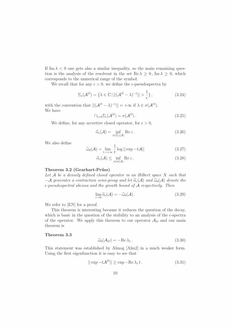
If Imλ < 0 one gets also a similar inequality, so the main remaining ques-tion is the analysis of the resolvent in the set Reλ ≥ 0 , Imλ ≥ 0, whichcorresponds to the numerical range of the symbol.

We recall that for any ǫ > 0, we define the ǫ-pseudospectra by

Σǫ(AD) = λ ∈ C | ||(AD − λ)−1|| > 1

ǫ , (3.24)

with the convention that ||(AD − λ)−1|| = +∞ if λ ∈ σ(AD).We have

∩ǫ>0Σǫ(AD) = σ(AD) . (3.25)

We define, for any accretive closed operator, for ǫ > 0,

αǫ(A) = infz∈Σǫ(A)

Re z . (3.26)

We also define

ω0(A) = limt→+∞

1

tlog || exp−tA|| (3.27)

αǫ(A) ≤ infz∈σ(A)

Re z . (3.28)

Theorem 3.2 (Gearhart-Pruss)Let A be a densely defined closed operator in an Hilbert space X such that−A generates a contraction semi-group and let αǫ(A) and ω0(A) denote theǫ-pseudospectral abcissa and the growth bound of A respectively. Then

limǫ→0

αǫ(A) = −ω0(A) . (3.29)

We refer to [EN] for a proof.This theorem is interesting because it reduces the question of the decay,

which is basic in the question of the stability to an analysis of the ǫ-spectraof the operator. We apply this theorem to our operator AD and our maintheorem is

Theorem 3.3ω0(AD) = −Reλ1 . (3.30)

This statement was established by Almog [Alm2] in a much weaker form.Using the first eigenfunction it is easy to see that

|| exp−tAD|| ≥ exp−Reλ1 t . (3.31)

10

Hence we have immediately

0 ≥ ω0(AD) ≥ −Reλ1 . (3.32)

To prove that −Reλ1 ≥ ω0(AD), it is enough to show the following lemma.

Lemma 3.4For any α < Reλ1 , there exists a constant C such that, for all λ s.t. Reλ ≤α

||(AD − λ)−1|| ≤ C . (3.33)

Proof : We know that λ is not in the spectrum. Hence the problem is justa control of the resolvent as |Imλ| → +∞. The case, when Imλ < 0 hasalready be considered. Hence it remains to control the norm of the resolventas Imλ→ +∞ and Reλ ∈ [−α,+α].

This is indeed a semi-classical result ! The main idea is that when Imλ→+∞, we have to inverse the operator

D2x + i(x− Imλ) − Reλ .

If we consider the Dirichlet realization in the interval ]0, Im λ2

[ ofD2

x + i(x − Imλ) − Reλ, it is easy to see that the operator is invertible byconsidering the imaginary part of this operator and that this inverse R1(λ)satisfies

||R1(λ)|| ≤ 2

Imλ.

Far from the boundary, we can use the resolvent of the problem on the linefor which we have a unifom control of the norm for Reλ ∈ [−α,+α].

ApplicationComing back to the application in superconductivity, one is looking at thesemigroup associated with AJ := D2

x + iJx−1 (where J ≥ 0 is a parameter).The stability analysis leads to a critical value

Jc = (Reλ1)− 3

2 , (3.34)

such that :

• For J ∈ [0, Jc[, || exp−tAJ || → +∞ as t→ +∞.

• For J > Jc, || exp−tAJ || → 0 as t→ +∞.

This improves Lemma 2.4 in Almog [Alm2], who gets only this decay for|| exp−tAJψ|| for ψ in a specific dense space.

11

3.3 Numerical computations

Here we reproduce in Figure 1 the classical picture due to Trefethen of thepseudo-spectra of the Davies operator D2

x + ix2 on the line and in Figure 2the corresponding picture realized with numerical computations for us byW. Bordeaux Montrieux for the case of Airy. W. Bordeaux Montrieux is us-ing eigtool3. These figures give the level-curves of the norm of the resolvent||(A−z)−1|| = 1

ǫcorresponding to the boundary of the ǫ-pseudospectra. The

right column gives the correspondence between the color and log10(ǫ).

As usual for this kind of computation for non self adjoint operators, weobserve on both figures, in addition to the (discrete) spectrum lying on thehalf-line of argument π

4(resp. π

3) , a parasite spectrum starting from the

fifteenth eigenvalue. This was already observed by B. Davies for the com-plex harmonic oscillator D2

x + i x2. This is immediately connected with theaccuracy of the computations of Maple.

The computation for Figure 2 is done on an interval [0, L] with Dirichletconditions at 0 and L using 400 “grid points”. The figure gives the level-curves of the norm of the resolvent ||(A− z)−1|| = 1

ǫcorresponding for each

ǫ to the boundary of the ǫ-pseudospectrum. The right column gives the cor-respondence between the color and log10(ǫ).In the upper part of the Airy-picture in Figure 2, these level-curves be-come asymptotically vertical lines corresponding to the fact that each ǫ-pseudospectrum of the Airy operator is a left-bounded half-plane.

The first zoom in Figure 3 below shows that for ǫ = 10−1, the ǫ-pseudo-spectrum has two components, the bounded one containing the first eigen-value. For ǫ = 10−2, the ǫ-pseudo-spectrum has three components, eachbounded one containing one eigenvalue. The second and third zoom illus-trate the property that, for a given k, as ǫ → 0, the component of the ǫ-pseudospectrum containing one eigenvalue µk becomes asymptotically a diskcentered at µk.

3see http://www-pnp.physics.ox.ac.uk/∼ stokes/courses/scicomp/eigtool/html/eigtool/documentation/menus/airy-demo.html and http://www.comlab.ox.ac.uk/pseudospectra/eigtool/

12

Figure 1: Davies operator: pseudospectra

0 20 40 60 80 100 120 140 160

−20

0

20

40

60

80

100

120

dim = 100

−7

−6

−5

−4

−3

−2

−1

0

Figure 2: Airy with Dirichlet condition : pseudospectra

13

Figure 3: Zooms

14

3.4 Higher dimension problems relative to Airy

Here we follow (and extend) [Alm2] Almog.

3.4.1 The model in R2

We consider the operator

A2 := −∆x,y + i x . (3.35)

Proposition 3.5

σ(A2) = ∅ . (3.36)

Proof : After a Fourier transform in the y variable, it is enough to showthat

(A2 − λ)

is invertible withA2 = D2

x + i x+ η2 . (3.37)

We have just to control for a given λ ∈ C, (D2x + i x + η2 − λ)−1 (whose

existence is given by the 1D result) uniformly in L(L2(R)) uniformly withrespect to η.

3.4.2 The model in R2+ : perpendicular current.

Here it is useful to reintroduce the parameter J , which is assumed to bepositive. Hence we consider the Dirichlet realization

AD,⊥2 := −∆x,y + i Jx , (3.38)

in R2+ = x > 0 .

Proposition 3.6

σ(AD,⊥2 ) = ∪r≥0,j∈N∗(λj + r) . (3.39)

Proof : For the inclusion

∪r≥0,j∈N∗(λj + r) ⊂ σ(AD,⊥2 ) ,

15

we can use L∞ eigenfunctions in the form

(x, y, z) 7→ exp i(yη + zζ)uj(x)

where uj is the eigenfunction associated to λj. We have then to use the factthat L∞-eigenvalues belong to the spectrum. This can be formulated in thefollowing proposition.

Proposition 3.7Let Ψ ∈ L∞(R2

+) ∩H1loc(R

2+) satisfying, for some λ ∈ C,

−∆x,yΨ + iJxΨ = λΨ (3.40)

in R2+ and

Ψx=0 = 0 . (3.41)

Then either Ψ = 0 or λ ∈ σ(AD,⊥3 ).

For the opposite inclusion, we observe that we have to control uniformly

(AD − λ+ η2)−1

with respect to η under the condition that

λ 6∈ ∪r≥0,j∈N∗(λj + r) .

It is enough to observe the uniform control as η2 → +∞ which results of(3.23).

3.4.3 The model in R+2 : parallel current

Here the models are the Dirichlet realization in R2+ :

AD,‖2 = −∆x,y + i J y , (3.42)

or the Neumann realization

AN,‖2 = −∆x,y + i J y . (3.43)

Using the reflexion (or antireflexion) trick we can see the problem as aproblem on R

2 restricted to odd (resp. even) functions with respect to(x, y) 7→ (−x, y). It is clear from Proposition 3.5 that in this case the spec-trum is empty.

16

4 A few theorems for more general situations

4.1 Other models

The goal is to treat more general situations were we no more know explicitelythe spectrum like for complex Airy or complex harmonic oscillator. At leastfor the case without boundary this is close to the problematic of the lecturesof J. Sjostrand. The operators we have in mind are (see [AHP])

D2x + (Dy −

1

2x2)2 + i c y , (4.1)

and the next one could be

(Dx +x3

3)2 + (Dy − x2y)2 + i c(x2 − y2) . (4.2)

More generally :

B(x, y) = Reψ(z) , Φ(x, y) = cImψ(z) , (4.3)

with ψ holomorphic will work.If ψ is a non constant polynomial and c 6= 0, then one can prove that theoperator will have compact resolvent (see Theorem 4.1 below).

4.2 Maximal accretivity

All the operators considered before can be placed in the following more gen-eral context. We consider in R

n (or in an open set Ω ⊂ Rn)

PA,V := −∆A + V , (4.4)

withReV ≥ 0 and V ∈ C∞(Ω),A ∈ C∞(Ω,Rn) .

Then it is interesting to observe that when Ω = Rn, then the operator is

maximally accretive (see [HelNi] for the definition). The proof which is givenin [AHP] is close to the proof (see for example [FoHel]) of the fact that if Vis in addition real −∆A + V is essentially self-adjoint.

17

4.3 A criterion for compactness of the resolvent

All the results of compact resolvent stated in this paper can be proved in anunified way. Here we follow the proof of Helffer-Mohamed [HelMo], actuallyinspired by Kohn’s proof in subellipticity (see [HelNi] for a presentation). Wewill analyze the problem for the family of operators PA,V , where the electricpotential has in addition the form :

V (x) =( ∑

j

Vj(x)2)

+ iQ(x) ,

with Vj and Q in C∞.We note also that it has the form :

PA,V =

n+p∑

j=1

X2j =

n∑

j=1

X2j +

p∑

ℓ=1

Y 2ℓ + iX0 ,

with

Xj = (Dxj− Aj(x)) , j = 1, . . . , n , Yℓ = Vℓ , ℓ = 1, . . . , p , X0 = Q.

In particular, the magnetic field is recovered by observing that

Bjk =1

i[Xj, Xk] = ∂jAk − ∂kAj , for j, k = 1, . . . , n .

We now introduce the quantities :

mq(x) =∑

ℓ

∑

|α|=q

|∂αxVℓ| +

∑

j<k

∑

|α|=q−1

|∂αxBjk(x)| +

∑

|α|=q−1

|∂αxQ| . (4.5)

It is easy to reinterpret this quantity in terms of commutators of the Xj’s.When q = 0, the convention is that

m0(x) =∑

ℓ

|Vℓ(x)| . (4.6)

Let us also introduce

mr(x) = 1 +r∑

q=0

mq(x) . (4.7)

Then the criterion is

18

Theorem 4.1Let us assume that there exists r and a constant C such that

mr+1(x) ≤ C mr(x) , ∀x ∈ Rn , (4.8)

andmr(x) → +∞ , as |x| → +∞ . (4.9)

Then PA,V (h) has a compact resolvent.

4.4 About the L∞-spectrum

We already met this question in Proposition 3.7. This proposition is actuallya particular case of the more general statement [AHP], which can be seen asgiving a comparison between the L∞-spectrum and the L2-spectrum.

Proposition 4.2We assume that V ∈ C0 and ReV ≥ 0 If (ψ, λ) satisfies

(PA,V − λ)ψ = 0 in D′(Rn) ,

with ψ ∈ L∞ (or L2), then either ψ = 0 or λ is in the spectrum of P = PA,V .

The proof is reminiscent of the so-called Schnol’s theorem.

5 Conclusion

What we plan to continue in collaboration with Y. Almog and X. Pan is toanalyze

1

tln || exp−tPA,V || ,

as t→ +∞ for our specific examples

1. in the case of the whole space,

2. in the case of the half space

3. and apply these results to the stability question of problem with bound-ary in various asymptotic limits.

19

This should lead to the introduction of critical fields like in the standardsuperconductivity theory (see [FoHel]). One of the difficulties for these gen-erallizations is that we have no longer the explicit knowledge of the spectrumlike for the complex Airy operator. We do not know for example if the spec-trum of the Dirichlet realization in the half-space asssociated with PA,V isnon empty.

References

[Alm1] Y. Almog. The motion of vortices in superconductors under theaction of electric currents. Talk in CRM 2008.

[Alm2] Y. Almog. The stability of the normal state of superconductors inthe presence of electric currents. Siam J. Math. Anal. 40 (2) (2008),p. 824-850.

[AHP] Y. Almog, B. Helffer, and X. Pan. Superconductivity near the nor-mal state under the action of electric currents and induced magneticfield in R

2. Preprint September 2009

[AHHP] Y. Almog, C. Han, B. Helffer, and X. Pan. Critical magnetic fieldand critical current of type II superconductors. In preparation.

[BJP] P. Bauman, H. Jadallah, and D. Phillips. Classical solutions to thetime-dependent Ginzburg-Landau equations for a bounded super-conducting body in a vacuum. J. Math. Phys., 46 (2005), p. 095104,25.

[Dav] B. Davies. Linear operators and their spectra. Cambridge Studiesin Advanced Mathematics.

[DSZ] N. Dencker, J. Sjostrand, and M. Zworski. Pseudospectra of semi-classical (pseudo)differential operators. Comm. Pure Appl. Math.57 (3) (2004), p. 384-415.

[EN] K.J. Engel and R. Nagel. One-parameter semi-groups for linearevolution equations. Springer Verlag.

[FoHel] S. Fournais and B. Helffer. Spectral methods in Superconductivity.To appear in Birkhauser.

20

[GGN] I. Gallagher, T. Gallay and F. Nier. Spectral asymptotics for largeskew-symmetric perturbations of the harmonic oscillator, Preprint2008.

[Han] C. Han. The eigenvalue problem for the Schrodinger operator withelectromagnetic field. Master Thesis (2009).

[Hel1] B. Helffer. Semi-Classical Analysis for the Schrodinger Operatorand Applications, no. 1336 in Lecture Notes in Mathematics (1988).

[Hel2] B. Helffer. The Montgomery model revisited. To appear in Collo-quium Mathematicum.

[HelMo] B. Helffer and A. Mohamed. Sur le spectre essentiel des opra-teurs de Schrodinger avec champ magntique, Annales de l’InstitutFourier 38 (2) (1988), p. 95-113.

[HelNi] B. Helffer and F. Nier. Hypoelliptic estimates and spectral theoryfor Fokker-Planck operators and Witten Laplacians. no. 1862 inLecture Notes in Mathematics, Springer-Verlag (2004).

[IvKo] B.I. Ivlev and N.B. Kopnin. Electric currents and resistive statesin thin superconductors. Adv. in Physics 33 (1984), p. 47-114.

[Mart] J. Martinet. Sur les proprietes spectrales d’operateurs non-autoadjoints provenant de la mecanique des fluides. These de doc-torat (in preparation).

[Sjo1] J. Sjostrand. Resolvent estimates for non-self-adjoint operators viasemi-groups. http://arxiv.org/abs/0906.0094.

[Sjo2] J. Sjostrand. Spectral properties for non self-adjoint differentialoperators. Provisory lecture notes for Evian 2009.

[Tr] L.N. Trefethen. Pseudospectra of linear operators. SIAM Rev. 39(3) (1997), p. 383-406.

[TrEm] L.N. Trefethen and M. Embree. Spectra and pseudospectra. Acourse in three volumes (2004-version).

[Vil] C. Villani. Hypocoercivity. To appear in Memoirs of the AMS.

21