DTIB FiLE COPYNASA Contractor Report 187443

co

ICASE INTERIM REPORT 14

SPECTRAL METHODS FOR TIME DEPENDENT PROBLEMS

Eitan Tadmor

NASA Contract No. NAS1-18605September 1990

INSTITUTE FOR COMPUTER APPLICATIONS IN SCIENCE AND ENGINEERINGNASA Langley Research Center, Hampton, Virginia 23665

Operated by the Universities Space Research Association

ELECTE t00T.2919MNASA sI^ a aLNational Aeronautics andSpace AdministrationLangley Research CenterHampton, Virginia 23665-5225

ICASE INTERIM REPORTS

ICASE has introduced a new report series to be called ICASE Interim Reports.The series will complement the more familiar blue ICASE reports that have beendistributed for many years. The blue reports are intended as preprints ofresearch that has been submitted for publication in either refereed journals orconference proceedings. In general, the green Interim Report will not be submit-ted for publication, at least not in its printed form. It will be used for researchthat has reached a certain level of maturity but needs additional refinement, fortechnical reviews or position statements, for bibliographies, and for computersoftware. The Interim Reports will receive the same distribution as the ICASEReports. They will be available upon request in the future, and they may bereferenced in other publications.

Robert G. VoigtDirector

Accession ForNTIS GRA&IDTIC TAB [Unannounced I]Justifioation

ByDistributionl.

Availability Codsvail and/or

Dist Speial

SPECTRAL METHODS FOR

TIME DEPENDENT PROBLEMS

Eitan Tadmor'

School of Mathematical Sciences, Tel-Aviv University

TABSTRACT

This short review on spectral approximations for time-dependent problems consists of

three parts. In part I we discuss some basic ingredients from the spectral Fourier and Cheby-

shev approximation theory. Part II contains a brief survey on hyperbolic and parabolic time-

dependent problems which are dealt with both the energymethod and the related Fourier

analysis. In part III we combine the ideas presented in the first two parts, in our study of

accuracy stability and convergence of the spectral Fourier approximation to time-dependent

problems. ( )

Lecture notes for the

Nordic Summerschool on Numerical Methods in Fluid Dynamics

August 20-25, 1990

Sydkoster, SWEDEN

'Research was supported in part by NASA Contract No. NAS1-18107 while the author was in residenceat the Institute for Computer Applications in Science and Engineering (ICASE), NASA Langley ResearchCenter, Hampton, VA 23665.

ti

TABLE OF CONTENTS

1. SPECTRAL APPROXIMATION THEORY 1

1.1. The Periodic Problem - Fourier Approximation 1

1.2. The Pseudospectral (Collocation) Approximation 8

1.3. Spectral and Pseudospectral Approximations - Exponential Accuracy 17

1.4. The Non-Periodic Problem - Chebyshev Approximation 19

2. TIME DEPENDENT PROBLEMS 29

2.1. Initial Value Problems of Hyperbolic Type 29

2.2. Initial Value Problems of Parabolic Type 36

2.3. Well-posed Time-Dependent Problems 38

3. THE FOURIER METHOD FOR HYPERBOLIC

AND PARABOLIC EQUATIONS 40

3.1. The Spectral Approximation 40

3.2. The Pseudospectral Approximation 50

3.3. Skew-Symmetric Differencing 54

3.4. Smoothing 55

Appendix. Fourier Collocation with Even Number of Gridpoints 62

V

1. SPECTRAL APPROXIMATION THEORY

1.1. The Periodic Problem - Fourier Approximation

Consider the first order Sturm-Liouville (SL) problem

d(1..1) - -"Ao(x), 0 < x < 27,-

augmented by periodic boundary conditions

(1.1.2) 0(0) = 0(2ir).

It has an infinite sequence of eigenvalues, Ak = ik, with the corresponding eigenfunctions

Ok(x) = eik= .Thus, (Ak = ik, Ok = eikz) are the eigenpairs of the differentiation operator

dxin L2[0,27r), and they form a complete system in this space. This system is complete

in the following sense. Let L2[0, 2-T) be induced with the usual Euclidean inner product

(1.1.3) (w(), w 2(X)) =- f0 wi (x)-(x)dx.

Note that k(x) are orthogonal with respect to this inner product, for

14. { o jk,(1.e.) (ek e = 2 = 2- j = k.

Let w(x)cL 2[0, 2r) be associated with its spectral representation in this system, i.e., the

Fourier expansion

(1.1.5) w(x) - E (k)k(X), 'i(k) -(wk)

k=-oo II€kII2

or equivalently,

(1.1.6) w(x) E ? b(k)ekx, ib(k) W(=)e- kt.

The truncated Fourier expansion

N1 . . )S NV W e z k ik

x ,

k=-N

denotes the spectral-Fourier projection of w(x) into 7rN-the space of trigonometric polyno-

mials of degree < N:

N

SNW = ,b(0) + Z[ib(k)e' + ib(-k)e- ikJk=1

N

(1.1.8) = 2(0) + Z[i[2(k) + 22(-k)] cos kx + i[2(k) - 2(-k)] sin kxk=1

N= Zatkcos kx + bk sin kx;

k=O

here hk and bk are the usual Fourier coefficients given by

ak = w(k) + i(-) 1 k) W() cos kd6,(1.1.9)

ik = 4(k) - fv(-k)] =ff jw )sin k~6.

Since w - SNW is orthogonal to the 7rN-space:

(1.1.10) (w - SNW, eikx) = 2ir(k)- 27ri(k) = 0, IkI _ N,

it follows that for any PNIEVr we have (see Figure 1)

(1.1.11) I1w - PNII 2 = 1w - SNWII2 + IISNw- PNI1 .

Hence, SNw solves the least-squares problem

SNW

Figure 1:

(1.1.12) 11w - SvwIl = Minp,,,,NjIW - pNII

2

i.e., SNW is the best least-squares approximation to w. Moreover, (1.1.11) with PN = 0 yields

(1.1.13) IISNWII = Ilwll2 - I1w - SNWII2 _ I1WI11

and by letting N --+ co we arrive at Bessel's inequality

(1.1.14) 27r E Izb(k)12 E Y i(k)l 110kJ 2 < lW 2l.k=-oo k=-oo

Remark: An immediate consequence of (1.1.14) is the Riemann-Lebesgue lemma, asserting

that

fo() = f d 70, for any weL2 [0,27r).

The system { k = eikx} is complete in the sense that for any w(x)eL 2[0,27r) we have

Parseval equality:

(1.1.15) 27, E it,(k)2 1 10(k)l'lkll"=ll1ll,k=-oo k=-oo

which in view of (1.1.13), is the same as

N

(1.1.16) lim IISNw =Z b(k)e?" - w(x)11 - 0.-N

The last equality establishes the L2 convergence of the spectral-Fourier projection, SNw(x),

to w(x), whose difference can be upper bounded by the following

Error Estimate:

11 W- SN 112 = I1W112 - IISNW 112 = 1 6i(k)l 2IlkIl = 27r E I,(k)l2.Ikl>N Ikl>N

We observe that the RHS tends to zero as a tail of a converging sequence, i.e.,27r

o w(x) - E 6(k)ei12 dx = 27r E I[b(k)I1-2 0.( k=-N Ikl>N N-.oo

The last equality tells us that the convergence rate depends on how fast the Fourier coeffi-

cients, ?b(k), decay to zero, and we shall quantify this in a more precise way below.

Remark (1.1.17) yields uniform a.e., convergence for subsequences; in fact one can show

Nv+(1.1.18) a.e._lim Iw(x) - SNpw(x)I = 0, inf L > 1.

3

In fact, w(x) = a.e. limNv. SNw(x) for all weL 2[0, 27.], but a.e. convergence may fail if w(.)

is only L' [0, 2ir]-integrable.

Yet, if we agree to assume sufficient smoothness, we find the convergence of spectral-

Fourier projection to be very rapid, both in the L' and the pointwise sense. To this we

proceed as follows.

Define the Sobolev space H-[0,27-) consisting of 2wr-periodic functions which their first

s-derivatives are L2-integrable; set the inner product

(1.1.19) (W1, w2)H. = t=oX DPwi(x)DPW2(x)dx.

The essential ingredient here is that the system {eikx} - which was already shown to be

complete in L2 [0, 2-r) - H[0, 27r), is also a complete system in H4[0,27r) for any s > 0. For

orthogonality we have

0 jfk,(1.1.20) (. ' I, eiJx)g, =

27r :L k p j =k.p=O

The Fourier expansion now readsoc

(11.1)W(X) .. E Cv,(k) e i kx

where the Fourier coefficients, iv,(k), are given by

(1.1.22) (k) - (w(x), e")H-

(eik, e k)H'

We integrate by parts and use periodicity to obtain

(w(x), ekx)H-J Dpw(x)DPe kxdx=

5

2"

p-0

=

- (_1)p(_ik) 2 p I/1 w(we-kQdp=O 0

and together with (1.1.20) we recover the usual Fourier expansion we had before, namely

(1.1.23) w 8o(k) = @(k) =

4

The completion of {e"'} in H[O, 27r) gives us the Parseval equality, compare (1.1.15)

S

Ow - SNwII'. = , >i: k(k)l2IlekI, H [ -i(k1 2ir> 2~Ikl>N Jkl>N P=O

(1.1.24)

N 2p • 27r. E I2,(k)12 = E _" I1w - SNWII 2 .p=O Jkl>N p=O

Since

2

(1.1.25) Const1 (1 + N) / ( NP) < Const 2(1 +

we conclude from (1.1.24), that for any weH'[O,2-r) we have

(1.1.26) 11 - SN I _< Const,. we"H[0,27r).

Note that Const, = Const, • IIw - SNWIIH -- 0. This kind of estimate is usually referedN-.-oo

to by saying that the Fourier expansion has spectral accuracy, i.e., the error tends to zero

faster than any fixed power of N, and is restricted only by the global smoothness of w(x).

We note that as before, this kind of behavior is linked directly to the spectral decay of

the Fourier coefficienLs in this case. Indeed, by Cauchy-Schwartz inequalityIIlwIIH. . IleikxllH, 1

I 2 (k)l = Ib(k)l _< IIew I l, .- Ile Ex0II) lWIl

(1.1.27)

1< Const +-(I + Ik12)"2

In fact more is true. By Parseval equality

00 0

llwll , = l lv(k)lIle'kllg = 2( k lt(k)l ,

k=-oo k Z=-O) IO

and hence by the Reimann-Lebesgue lemma, the product (l+lkl)1Ilz(k)I is not only bounded

(as asserted in (1.1.27), but in fact it tends to zco,

(1 + IkI2)!2Vo(k)l- 0.k-+00o

Thus, f,(k) tends to zero faster than ikl - for all w(x)cH o. This yields spectral convergence,

for

11 W SNW112 = 27r E 1? (k)12 _< Const. 1 < Const.Ikl>N Jk >N ( 1 + 1k 2)' IVo s -1

5

i.e., we get slightly less than (1.1.26),

11W SNW 1 :-- ---t. 0 s > .I~w-s, ll <¢ N 3-2._ N-.oo

Moreover, there is a rapid convergence for derivatives as well. Indeed, if w(x)eH'[0, 2r)

then for 0 < a < s we have

11w - SNWII = (2'r >k 2p)11(k )12

Ikl>N p=O

" Const. E (1 + IkI2)yib(k)12

Ikl>N

_ ~(1 ±+ Ikl2)"" Const. E (1 + N -2) IW(k)1 2 <

Ikl>N ( 2,O

" Const. E (1 +,r- " P- - (k)I 1

Ikl>N (1 + N 2 )s-a

K Const.11W,- 2(sGVWll- N2(s-a)

Hence1

(1.1.28) 11W - SNwllHo < Const,. N<-. o- _ s, weH8 (0,2r)

with Const, JJW - SNWIIH. - 0. Thus, for each derivative we "lose" one order in theN--f 00

convergence rate.

As a corollary we also get uniform convergence of SNw(x) for H'[0, 27r)-functions w(x),

with the help of Sobolev-type estimate

(1.1.29) Maxo<.< 2.-lv(X)< Const.lvllH, .

(Proof: Write v(x) = U(xo) + fxo v'(x)dx with U(x0 ) = f02 v(x)dx, and use Cauchy-

Schwartz to upper bound the two integrals on the right.)

Utilizing (1.1.20) with v(x) = w(x) - SNw(x) we find

Maxo <2,,u(x) - SNw(X) < Const.I u SNwllj,,(1.1.30) 1

< Consto,---- 0, wcHl[(0, 27r).NS - 1 N.oo

Corollary: Assume w(x)H'[O, 27r). Then

00(1.1.31) ,(x) = ()k-c-o

6

In closing this section, we note that the spectral-Fourier projection, SNw(x), can berewritten in the form

SNw( ) E 2_, (k)e = 2" w( ) E e'k(x-C)d6(1.1.32a) k--N

f 27rO D,(, -)(6dC0

where

(1.1.32b) DN(x - 1 N - sin2 2k=-N 27.-r) sin (j~

Thus, the spectral projection is given by a convolution with the so-called Dirichlet kernel,

(1 .1 .3) D~~ z) = -- in2ir sing

Now (1.1.23) reads

(1.1.34) Jw(x) - DN(x) *w(x) < Const, • Const, - JJ8 JJ'f'.

7

1.2. The Pseudospectral (Collocation) Approximation

We have seen that given the "moments"

jb(k) 2-='z2(kJ,=' w(we-'ked , -N < k < NV,

we can recover smooth functions w(x) within spectral accuracy. Now, suppose we are given

discrete data of w(x): specifically, assume w(x) is known at equidistant collocation points

(1.2.1) W,=W(X,), X,=T+vh, V=0,1,...,2N.

Without loss of generality we can assume that r-which measures a fixed shift from the origin,

satisfies

h 2,r(1.2.2) 0 < N±1h2N+l1

Given the equidistant values w,, we can approximate the above "moments," CV(k), by the

trapezoidal rule 2

h 2N+I -ikx_ 1 2N

(1.2.3) E -= ,,= 2N + 1 =0

Using zi(k) instead of ? (k) in (1.1.7), we consider now the pseudospectral approximation

N

(1.2.4) 'ONW= v(k)ek=-N

The error, w(x) - ONw(x), consists of two parts:

W(X) - ?NW(X) = b (k), i' + E [C(k)- (k)]e

IkI>N IkI<N

The first contribution on the right is the truncation error

(1.2.5) Tw~(x) =(I- SN)w(x) = ? .(k)e' .

Ikl>N

We have seen that it is spectrally small provided w(x) is sufficiently smooth. The second

contribution on the right is the aliasing error

(1.2.6) ANW(X) = 5 [zV(k) - I(k)]e "

Ikl<N

This is pure discretization error; to estimate its size we need the

2 ' and E" indicate summation with 1 of the first and respectively, the first and the last last terms.

8

Poisson's Summation Formula (Aliasing)

Assume w(x)eH'[0, 27r). Then we haveCo

(1.2.7) ib(k) = 1 eiP(2N+l)r,6)(k + p(2N + 1)).

Proof: For w(x)cH' [0, 2-r) we insert its Fourier expansion

1 2N 2N ;X(1.2.8) f(k) =2N + 1 Z v(je)e- - 1 Z(je _, 2N +1 ,= o E

Since w(x) is assumed to be in H', the summation on the right is absolutely convergent

(1.2.9) E li(j)l _ (! + j 2)It(j)2 . 1 Const.'1wIHi,-7=-00

and hence we can interchange the order of summation

1 0 2N

(1.2.10) T(k) = 2N + 1 E ?(j) E ej=-00 V,=O

Straightforward calculation yields2N ~2N 21 2N -ii~~~ . e(jk),,_3.' -

21V + I = 'ik(+')" Jt) 2N + I V=o

(1.2.11) ei(j-k) 2 ,r.(2N+1) 1+12N+ =0 j-k#0[mod2N+1)

2N + 12N+ 1, j-k =p. (2N+ 1).

and we end up with the asserted equality

00 1 2N oo,(= 5 )(J) 2N+1 ei(k) = + e(k + p(2N + 1)) ' e'P(2N+

J=--00 0=,=0- 0

We note that once w(x) is assumed to be smooth, it is completely determined (pointwise,

that is) by its Fourier coefficients tb(k); so are its equidistant values w, - w(x,) and so are

its discrete Fourier coefficients iv(k). The last formula shows that fv(k) are determined in

terms of Cv(k), by folding back high modes on the lowest ones, due to the discrete resolution

of the moments of w(x): all modes = k[mod2N + 1] are aliased at the same place since they

are equal on the gridpoints

(1.2.12) e-( +p

( 2 N +1

) )x= e ip(2N+1)r

• e'kt-.

9 t

Let us rewrite (1.2.7) in the form

@(k) = v(k) + Z etP(2N+I)r -a(k + p(2N + 1)).p;o

Returning to the aliasing error in (1.26), we now have

(1.2.13) Avw(x) = [Zelp.(N) w?(k +p (2N +1))] ei.

We note that TNw(x) lies outside 7rN while ANw(X) lies in 7rN, hence by H'-orthogonality

[Iw(x) - ¢bNw(x)II& = E (1 + [kl 2)' . I@(k)12 -- truncationIki>N

+ E (1 + [kj 2 ), I E eip(2N+I)r -v(k + p(2N + 1))12 <- aliasing.Ikj<N Poo

Both contributions involve only the high amplitudes - higher than N in absolute value; in

fact they involve precisely all of these high amplitudes. This leads us to aliasing estimate

> (1 + Ikl2)qI E eip(2N+)" .t(k + p(2N + 1))12 <Ik!<N p O

1 : (1 + lk + p(2N + z12)l )°I(k + p(2N + 1))12.

Ik<N p-o

(1.2.15) M xk 5 [ 1 + k 2 <• alk, NP 1 + Ik + p (2 + 1)12] -

jjTNW(X)112 . . Eo 1 +N 2

Hence, we conclude that for any s > 1. we have1

(1.2.16) IIANw(x)IIHI < Const -IITNw(x)IIH,, s >

Augmenting this with our previous estimates we end up with spectral accuracy as before,

namely11

(1.2.17) 11w - kNWIIHc < Const, N' weH8 [0,27r), s _u>

We observe that bNw(x) is nothing but the trigonometric interpolant of w(x) at the equidis-

tant points x = x,:N 2N i x I x¢V)(x).=x,. = E- 1 E w(x,) e =

k=-N V =(1.2.18)

2N 1 Nj

= E w(x,) 2N + 1 > ek(P'-)h " W(xp).V=O k=- N

10

This shows that OV is in fact a seudospectral projection, which in the usual sin-cos formu-

lation reads

N

?/INw = 'ak cos kx + ik sn kxk=O

(1.2.19) r ~ ~ ak ] w(x,) [Cos hx",[bk J 2N + 1 _ L sinkx,, "

Thus, trigonometric interpolation provides us with an excellent vehicle to perform approxi-

mate discretizations with high (= spectral) accuracy, of differential and integral operations.

These can be easily carried out in the Fourier space where the exponents serve as eigenfunc-

tion. For example, suppose we are given the equidistant gridvalues, w,, of an underlying

smooth (i.e., also periodic!) function w(x), w(x)cH'[O, 27r). A second-order accurate discrete

derivative is provided by center differencing

dw += X) - W-1 + 0(h2 ).T(X 2h

Note that the error in this case is, 0(h 2 ) = w( 3)(c)h 2 , no matter how smooth w(x) is.

Similarly, fourth order approximation is given via Richardson procedure by

dw (X = 8[)W - [W +2 - W v-2 + O(h 4 ).

X 12h

The pseudospectral approximation gives us an alternative procedure: construct the trigono-

metric interpolant

N 1 2N

(1.2.20) OArw(x) = E i-v(k)e ' x, t = 2N + 1 Z w1 ek=-N 0

Differentiate - in the Fourier space this amounts to simple multiplication since the exponen-

tials are eigenfunctions of differentiation,

(1.2.21) TONw(X)= f J(k)iketkz,dx k=-N

and we approximate

(1.2.22) dw X ) = d ()x + spectrally small error.

Indeed, by our estimates we have for w(x)eH'[O,27r),s > 1,

(1.2.23) Maxo<=<2,l dw(x) - dNW(x)l _ Const.11w(x)- CNw(o)st < 8---t-

- TCs11 N- 2

which verifies the asserted spectral accuracy. Similar estimates are valid for higher deriva-tives. To carry out the above recipe, one proceeds as follows: starting with the vector ofgridvalues, ib = (wO,. , w2,v), one computes the discrete Fourier coefficients

1 2N

(1.2.24) V(k) 1 -N _ N < N

or, in matrix formulation

iD(- ) O1 ikXL,.(1.2.25) F Fk ,= eN+1

then we differentiate

(1.2.26) ib(k) --+ ikzi(k),

or in matrix formulationz (-N) fv(-N) -iN

(1.2.27) [ :h] A="

ib(N) J(N) iNand finally, we return to the "physical" space, calculating

N(1.2.28) sib(k)e' v 0,1,...2N,k--N

or in matrix formulation

(1.2.29) [ = F*.(2N+1) : (2N+l)Fk ,e kx.dw IXN ~ bN

The summary of these three steps is

(1.2.30) :O D : O D -= (2N + 1)F'AF,S'(XN) W2N

where ObD represents the discrete differentiation matrix, and similarly ObD' for higher deriva-

tives.

Note: Since (2N + 1)F*F = I2N+1 (interpolation!) we apply 'bDS = (2N + 1)F*A"F. Howdoes this compare with finite differences and finite-element type differencing?

12

In periodic second-order differencing we have

0 1 0 -1-1 0 0

FD2 2h

0 0 11 0 -1 0

fourth order differencing yields

0 8 -1 1 -8-8 0 1

FD4 = .-12h -

-1 0 8

8 -1 1 -8 0

In both cases the second and fourth order differencing takes place in the physical space.

The corresponding differencing matrices have finite bandwidth and this reflects the fact that

these differencing methods are local. Similarly, finite-element differencing,

1 1 4 1 1 1 WV+1 - WV-1

6 -/ + W + v = 2h

corresponds to a differencing matrix

4 1 1 -1

6 "0 1 ... 0 -1-1 0 0

FE4 = 6 *6 2h0 0 1

1 1 4 1 0 . -1 0

We still operate in physical space with O(N) operations (tridiagonal solver) and locality

is reflected by a very rapid (exponential decay) away from main diagonal. Nevertheless, if

we increase the periodic center differences stencil to its limit then we end up with global

pseudospectral differentiation

d N ( ik 2N ik kV;

(1.2.31) dx =W( -) E 2N -+1 "eX k=-N =

recall the Dirichlet kernel (1.1.33)

Ni ei(2N+l )x sin(N + 1)x(1.2.32) E e e eiX - 1 sin

k=-N

13

and its derivative,Ndsin(N + =) (Nv+ + - cs.

N)dsi(N+ )x (N+) cos(N+ 1)x sinE- 1 cosEsin(N + 1)x(1.2.33) ike' x -2- = 2_2_x -- 2-2

k=-N dx sin sin2

so that

( kk(vp)h (N + }) cos((N + .)(v - )h( 1 .2 .3 4 )k = i k e i k " ' h 2i (

k= -N sin( xv~)

Hence (1.2.31), (1.2.34) give us

d N1 (-1)" ,1 -'D, s(1v'-)(1.2 .35 ) W '( .,) d O NW (X ) = 2 i ( ) V xu W -.

TX U=o2 sin2: 2 xl 2 sin( 2x)'

In this case bD is a full (2N + 1) x (2N + 1) matrix whose multiplication requires O(N 2)

operations; however, we can multiply ObD[w] efficiently using its spectral representation from

(1.2.30),

"OD = (2N + 1)F*AF.

Multiplication by F and F* can be carried out by FFT which requires only O(N log N)

operating and hence the total cost here is almost as good as standard "local" methods, and

in addition we maintain spectral accuracy.

We have seen how the pseudospectral differentiation works in the physical space. Next,let's examine how the standard finite-difference/element differencing methods operate in

the Fourier space. Again, the essential ingredient is that exponentials play the role of

eigenfunctions for this type of differencing. To see this, consider for example the usualsecond order center differencing, D2 (h), for which we have(1.2.36) =k eik+l - e- ik -1 isin(kh) eik,

(1h2.36)=2h = h e

The term i is called the "symbol" of center differencing. By superposition we obtainh

for arbitrary grid function (represented here by its trigonometric interpolant)

N

(1.2.37) ?PNW(X) = ib(k)e ik

k=-N

that

WV+ I - Wt, 1 N2h = D2(h)¢PlNw = v(k)D(h)eikx=x.

k=-N(1.2.38)

N isin(kh), - k x

= E h (k)eIk--x.k=-N

14

It is second-order accurate differencing since its symbol satisfies

(1.2.39) isin(kh) = ik + .(k 3h2 ).h

Note that for the low modes we have O(h 2) error (the less significant high modes are differ-

enced with 0(1) error but their amplitudes tend rapidly to zero). Thus we have

d 11 = sin(kh), 2II d7NW- D2(h)?NW E Ik - - I Ii(k)h

(1.2.40) k=-N

< Const.h ' E (1 + Ikl)lt,(k)l2 < Const.h' - II/)NW113,,

and this estimate should be compared with the usual

-W(X,) - 2h < os'h.Mx, ()dx 2

The main difference between these two estiamtes lies in the fact that (1.2.41) is local, i.e.,

we need the smoothness of w(x) only in the neighborhood of x = x1, and not in the whole

interval. The analogue localization in the Fourier space will be dealt later.

Similarly, we have for fourth order differencing the symbol

.1 4 sinkh sin2kh]S[4 sh - 2hJ = ik + o(k5 h4 ).

In general, we have difference operators whose matrix representation, D, is of the form

(1.2.41) D = (dik] -N < j,k < N

and it is periodic and antisymmetric (here [=] =[mod 2N + 1])

(i) periodicity djk = dfk-j]

(1.2.42)(ii) antisymmetry dk = -dkj.

Matrices satisfying the periodicity property are called circulant, and they all can be diago-

nalized by the unitary Fourier matrix

(1.2.43) D = U*AU, U = (2N + 1)2 . F, U*U = '2N+.

15. . .. . . . . . . . . . .

Indeed, with p - q = t we have

1 N[U*DU]jk 2N + 1 Z e -q]e-

p,q-N

1 N2N + 1 4q=-Nr

(1.2.44) 1 N ijh N i(k-.).(r+qh)- 2N E e eid[ q E e-i~-)(+h

2N + 1 -,q-N q=-NI j#k,

- ikh d[]j = k,

and using the antisymmetry we end up with symbols Ak

N(1.2.45) A = diag(AN,... ,AN), Ak = 2i dtsin(kUh).

1=1

As an example, we obtain for the finite-element differencing system

.sinkh (4 1 ,kh +Ak = 2-h + e 6 e-

(1.2.46) 6i sin(kh)

h 4 + 2 cos(kh)ik+O(h).

In general, the symbols are trigonometric polynomials or rational functions in the "dual

variable," kh, which has "exact" representation on the grid in terms of translation operator

(polynomials or rational functions), and accuracy is determined by the ability to approximate

the exact differentiation symbol ik foriki - 1, see Figure 2.

16

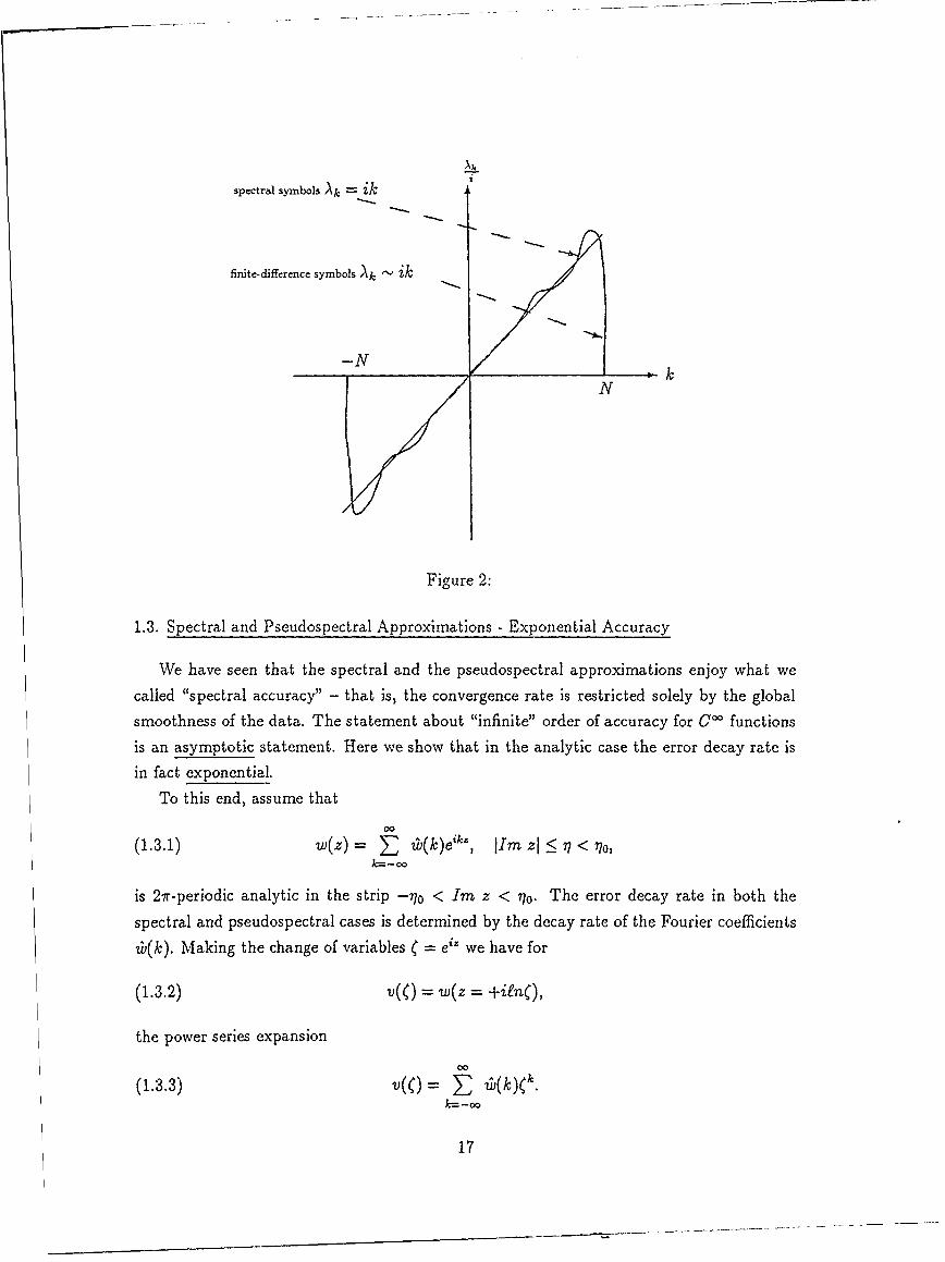
spectral symbols Ak - ik

finite-difference symbols Al, i"

-N __ k

V

N

Figure 2:

1.3. Spectral and Pseudospectral Approximations - Exponential Accuracy

We have seen that the spectral and the pseudospectral approximations enjoy what we

called "spectral accuracy" - that is, the convergence rate is restricted solely by the global

smoothness of the data. The statement about "infinite" order of accuracy for Co functions

is an asymptotic statement. Here we show that in the analytic case the error decay rate is

in fact exponential.

To this end, assume that

00

(1.3.1) w(z) = i T(k)e"', Iml zl < 7 < no,k-_o

is 27r-periodic analytic in the strip -n1o < Im z < 710. The error decay rate in both the

spectral and pseudospectral cases is determined by the decay rate of the Fourier coefficients

?b(k). Making the change of variables C = eiz we have for

(1.3.2) v(() = w(z = +ien(),

the power series expansion

(1.3.3) V()= S (k)(k .

k7 -co

By the periodic analyticity of w(z) in the strip IImzl : q < 77o, v(C) is found to be single-

valued analytic in the corresponding annulus

(1.3.4) e-M < I17 < e°,

whose Laurent expansion is given in (1.3.3):

(1.3.5) = IV (C )-(k+l)d(, e- 0 < < e0.

This yields exponential decay of the Fourier coefficients

(1.3.6) ji'(k)I < M(rl)e-k, M(77) = Maximzi, <w(z)I, 0 < 7 < 770.

We note that the inverse implication is also true; namely an exponential decay like (1.3.6)

implies the analyticity of w(z). Inserting this into (1.1.24) yields

11w - SNwII2 = 27r E 1I?(k)l2 <Ikl>N

(1.3.7)

< 27r. M2 (27). 5 e-2 = 2 7 - I. -- 2n:kl>N e2n - 1

and similarily for the pseudospectral approximation

(1.3.8) 11w - tPNW 12 <Const. M2 () e- n.

Note that in either case the exponential factor depends on the distance of the singularity

(lack of analyticity) from the real line. For higher derivatives we likewise obtain

(1.3.9) 11W - SNW IH + 11w - ONWII H < Const.N ° M2 (y) e2 N-- e2n - "

We can do even better, taking into account higher derivatives, e.g.,

(1.3.10) kilv(k) = 1L (dv -dC

so that with

(1.3.11) M,(-q) = en 7 MaxjC=Ilv)((),j=0

we have

(1.3.12) kl6b(k)l _< MI(77)e -'n,

and hence

(1.3.13) 11W - SNWII'fH, + I1w - OPNW11,Io < Const.M,(, 7)e-,-

18

1.4. The Non-Periodic Problem - Chebyshev Approximation

We start by considering the second order SL problem

2d 2d(1.4.1) -,-- ) = A,¢(X), -1 < X < 1.

This is a special case of the general SL problem

(1.4.2) L( = - () + q(x)¢(x) = AO(x), p, q, w > 0.

Noting the Green identity

(1.4.3) (LO, ),(x)= -(pb')'+ qc =p(x)[b, 11' + (V), Lo),(x), [V), 01 = b' - 00',

we find that L is formally self-adjoint provided certain auxiliary conditions are satisfied. In

the nonsingular case where p(a) -p(b) 0 0, we augment (1.4.2) with homogeneous boundary

conditions,

(1.4.4) (a) = O(a) = 0, b(b) = q(b) = 0.

Then L is self-adjoint in this case with a complete eigensystem (Ak,lkk(x)): each

w(x)eL (x)[a, b] has the "generalized" Fourier expansion

(1.4.5) w(x) 2v(k)Vk(x), fv(k)= ( )()k=O 1lOk(X)llL

with Fourier coefficients

(1.4.6) T(k) ) O()k(b)w(x)dx.

The decay rate of the coefficients is algebraic: indeed

Iii~kIII - (Li/k, w)=

(1.4.7) TI-¢i-" (p(x)" [¢/, wlb + (a ,Lw)

- i (p(). a l1 L(j)w)Ib L(O)w),.

W j=O "k A

The asymptotic behavior of the eigenvalues for nonsingular SL problem is

Ak 1rk , Const.k2

19

and hence, unless w(x) satisfies infinite set of boundary restrictions we end with algebraic

decay of C(k)1 p~) ~b(x~wx)I~ Const.

This leads to algebraic convergence of the corresponding spectral and pseudospectral pro-

jections.

In contrast, the singular case is characterized by having, p(a) = p(b) = 0, in which case

L is self-adjoint independently of the boundary conditions since the brackets , j drop, and

we have spectral decay-compare (1.1.22)

(1.4.8) Th(k)- 1 _ .. (gk,L(S)) < 1 IIL(°)wII:Ik lWkllw W - 1141wkl

provided w(x) is smooth enough; that is, the decay is as rapid as the smoothness of w(x)

may permit.

Returning to the singular SL problem (1.4.1) we use the transformation

d 1 d 1 d(1.4.9) x = cos9, =

which yields

d 2

(1.4.10) d921 €(O) = )€(9), $(9) b=O(cos9),

obtaining the two sets of eigensystems

(1.4.11a) (AA = k 2 ,¢, = cos k9),

and

(1.4.11b) (Ak = k 2,q¢k = sin kO).

The second set violates the boundedness requirement which we now impose

(1.4.12) lo'(-11)1 <Const.,

and so we are left with

(1.4.13) (Ak = k2, k(x) = cos(kcos - 1 x)).

The trigonometric identity

cos(k + 1)0 = 2 cos 0 cos k0 - cos(k - 1)0

20

yields the recurrence relation

(1.4.14) Vbk+l(x) = 2xo;k(x) - kk-1(x), ?ko(x) -1,()= x ,

hence, ?Pk(x) are polynomials of degree k - these are the Chebyshev polynomials

(1.4.15) Tk(x) = cos(k cos-1 x)

which are orthonormal w.r.t. Chebyshev weight w(x) = (1 - 2 -!-

0 h#I,

(1.4.16) (T(x),Tj(x)), = -Tk(X)(x) = IITII, = j = k > 0,

IToI12 = 7 = =0.

In analogy with what we had done before, we consider now the Chebyshev-Fourier expansiono

(1.4.17) w(x) ,- E ^(k)Tk(x), zb(k) = ( 2(x),Tk(x)),

k=O V1TAWt

To get rid of the factor 1 for k = 0 we may also write this as2

(1.4.18a) w(X) ,. E '?b(k)Tk(x)

k=O

where

(1.4.18b) Cv(k) = (w(x), Tk(x)). = 2 1 w(x) cos(k cos' x)dx(1.4./4) ( ir= J V -X2

or using the above Chebyshev transformation

(1.4.18c) ti(k) =2 f w(cos ) cos k d .

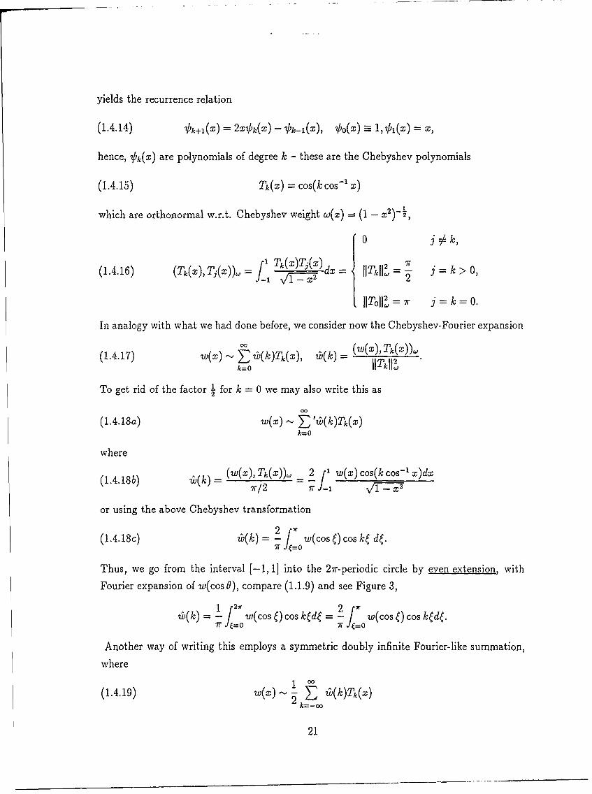
Thus, we go from the interval [-1, 1] into the 27r-periodic circle by even extension, with

Fourier expansion of w(cos 0), compare (1.1.9) and see Figure 3,

I =_ w(cos ) cos k~d = _ w(cos ) cos k d.7.", =0 7r" J=0

Another way of writing this employs a symmetric doubly infinite Fourier-like summation,

where

1 0o(1.4.19) w(X) , -2 E 6(k)Tk(X)

21

W(O) = w(x = cosO)

X = cos8

/0 +1

w(O) =W(-9)

Figure 3:

with Tk(x) Tk(x) and

(1.4.20) ti(k) = 2(1 w(x)Tk(X) dx-J v - dx, -cc<k <c.

The Parseval identity reflects the completeness of this system

IIW(X)II1' w 2(x)dx I 1 l4D1a 2~ + 1,Ci(1.4.2.1)4LkO J

T ooIti(k)2

k=O

which yields the error estimate

IIW - SNWIIT = 1- S Iv(k)I2.4 k>N

Now, in order to get a measure of the spectral convergence we have to estimate the decay

rate of Chebyshev coefficients in terms of the smoothness of w(x) and its derivatives; to

this end we need Sobolev like norms. Unlike the Fourier case, {Tk(x)} is not complete with

respect to H8 - orthogonality is lost because of the Chebyshev weight. So we can proceed

formally as before, see (1.1.24),

(1.4.22) I1W - SNWII = 27r E ItC(k)l < (1 + Ik12) 12k>N k>N (1 + N 2 )s

i.e., if we define the Chebyshev-Sobolev norm

"o

IIW112. = -(I + Ik 12 jl,(k)1 2,k=O

22

then we have spectral accuracy

11W - SNWIIT: Const,* weH -1, 1].

In fact the H space can be derived from appropriate inner product in the real space as done

in Fourier expansion. The correct inner product is given by - compare (1.1.19)

( L ) 2r d 2p d 2p(1.4.23) (W-,W2)Hf. - EW 1 COS0 Wcos

p=O x=cos P=O.

so that0 j 0 ,

(1.4.24) (TkTj)H2, = , I,(1.4.24)~_ ET' i H' - k4p, =k (with -, factor at j =k =0).

Hence the Fourier coefficients in this Hilbert space behave like00

(1.4.25) (w(x),Tk)H . - E(1 + k2 )2,ii(k),k=O

and the corresponding norm is equivalent to

(1.4.26) Ip~ E(1 + k2) l7b(k)12 .k=O

The reason for the squared factors here is due to the fact that L is a second order differential

operator, unlike the first-order D A A in the Fourier case, i.e.,

(1.4.27) E(1 + Ikl2)2 li(k)I J ~ ILw w Tk=O p=O

involves the first 2s-derivatives of w(x) - appropriately weighted by Cliebyshev weight. This

completes the analogy with the Fourier case, and enables us to estimate derivative as well-

compare (1.1.28 - 1.1.29),1

(1.4.28) 11w - SNWII1 < Const 8 -. _, o<s, weH [-1,1].

Next, let's discuss the discrete setup. Because we seek an even extension of the upper semi-

circle we consider the case of even number of grid points - equally distributed along the unit

circle. One choice is to look at

9V = r + vh = (v + )r (h = -,r =h)

23

0 1. .'

X, cos[(v + T1)]

Figure 4:

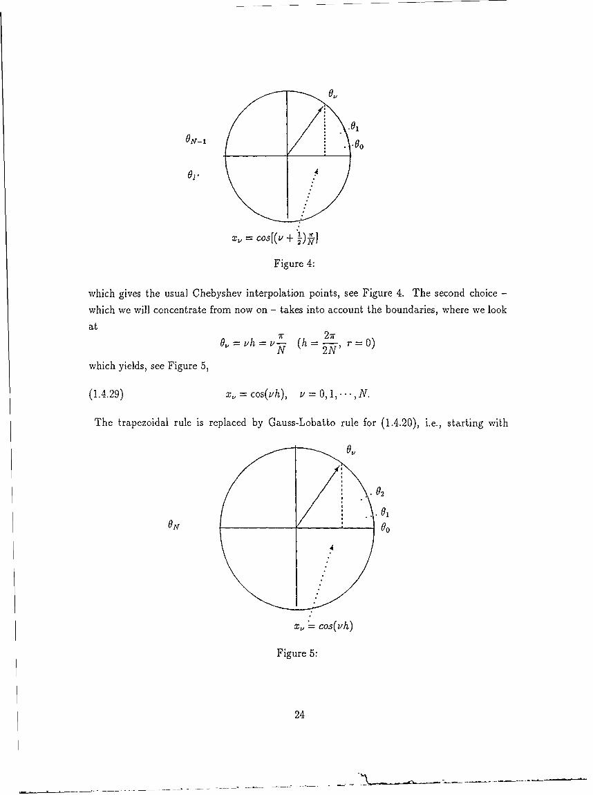
which gives the usual Chebyshev interpolation points, see Figure 4. The second choice -

which we will concentrate from now on - takes into account the boundaries, where we look

at iro = ,h =V7, (h = "- , r,--o)2Nr

which yields, see Figure 5,

(1.4.29) X, = cos(vh), v = 0,1,... ,N.

The trapezoidal rule is replaced by Gauss-Lobatto rule for (1.4.20), i.e., starting with

0V

02.. 01

X, cos(vh)

Figure 5:

24

(1.4.18c), we have2S 2

(1.4.30) w(k)=- w(cos 6) cos k~d6 - - I"w(cos 0,) cos kO, •4K L" =0 Wi N=-

and we end up with the discrete Chebyshev coefficients

2 N(1.4.31) iv-(k) = - WTk(x,), 0 < k < N.

Indeed, this corresponds to the case of Fourier interpolation with even number of equidistant

gridpoints 0,, in (A.1.2), for

1 2N 1 N

=bk Z 1: -11eik" -E wik, + e ikO.] 27r=

= 2 "w,cos(k0z).

Then one may construct the Chebyshev interpolant at these N + 1 gridpoints

N(1.4.32) lkNW(X) = E "i(k)Tk:(x).

k=O

We have an identical aliasing relation

(1.4.33) ?i(k) = E zb(k + 2pN)

(compare A.1.5), and hence spectral convergence, i.e., (compare (1.2.14) and (1.2.12))

(1.4.34) IlW(X) - V)NW(X)IIH, -- Const , -. weH , s > o,

where Const. -, IWIH,.

Example: We have the Sobolev imbedding of LOO space

1_ [ 1('(kk) 1)

w(x)1_ I-(k)! < - (E1l + k I2)-'I(k)l 2 1k=- 2 k

< Const. II-wIIH,, a > 1

Consequently,

MaxIw(x)- INW(x)l < (Const, Ilwlliw) - S > 0'> .

2N-0 2

25

In particular, with s = N + 1 we obtain the "usual" estimate for the near minmax approxi-

mation ( collocated at at x, = cos + )

e-_NMax.lw(x) - ,bvw(x)I Const.lwlHN+ •

T N!

We briefly mention the exponential convergence in the analytic case. To this end we employ

Bernstein's regularity ellipse, Er, with foci ±1 and sum of its semi axis = r. Denoting

(1.4.35) M(77) = Max.,,.I-(z)j, r = e7.

We have

Theorem. Assume w(x) is analytic in [-1,1] with regularity ellipse whose sum of semiazis

- = e", > 1. Then

IIw(X) - ¢Nw(x)iI° + IIw(X) - SIW(x)2 <-Const.M-H H o e2 "j - 1 "

Proof: The transformation z = (C + -')/2 takes Eo from the z-plane into the annulus

To < I(I < ro in the (-plane. Hence, v(() = 2w (z = admits the power expansion

(1.4.36) v(C) = 2w (C ) i vyk, r- ) < I < ro ==-oo

indeed, setting ( = e' 6 and recalling Cv(-k) = z(k), the above expansion clearly describes

the real interval (-1,1]

o

(1.4.37) w(z = cos 0)= E' i(k)coskO.k=O

By Laurent expansion in (1.4.36)

(1.4.38) 1k) = d( i r TC, e 10 < r < 00,2x1CIk+1

hence

(1.439) It'(k)l <! M (77)e - k,7

and the result follows along the lines of (1.3.7-8).

Finally, we conclude with discussion on Chebyshev differencing. Starting with grid values

w/ at Chebyshev points x( = cos .), one constructs the Chebyshev interpolant

N 2 N(1.4.40) ONW(X) = "iV(k). Tk(X), iV(k) = . _ "wLcos(kx1 ,).

k=O z'v0

26

One can compute 7i(k), 0 < k < N, efficiently via the cos-FFT with O(N log N) operations.

Next, we differentiate in Chebyshev space

d N d(1.4.41) k (x)- E"(k)-Tk(x).(.1 d=O

In this case, however, Tk(x) is not an eigenfunction of J; instead JTk(x) - being a polyno-mial of degree < k - 1, can be expressed as linear combination of {Tj(x)}j.- (in fact Tk(x)

is even/odd for even/odd k's): with co = 2, ck>o = 1 we obtain

d 2(1.4.42) -Tk(x) = - o_ T 3 (X)(1.442)dx Ck o~<<A

h --3 odd

and hence(1.4.43) dNW(X) - (k 2(X).

A-7 odd

Rearranging we get

d N 2(1.4.44) T'/Nw(x) = _"' i'(k)Tk(x), V'(k) = - E pih(p)

k=o Ck _p+1h odd

and similarly for the second derivative

(1.4.45) ibv"(k) = 2 p(p2 -kV)v(p).Ck pkh+2

p+h even

The amount of work to carry out the differentiation in this form is O(N 2 ) operations which

destroys the N log N efficiency. Instead, we can employ the recursion relation which follows

directly from (1.4.44)

(1.4.46) ib'(k + 1) = fv'(k - 1). Ck_1 - 2kzl(k).

To see this in a different way we note that

sin(k + 1)0 = sin(k - 1)0 + 2 sin 0 cos k9,

which leads toI dTk+1 I I. dTk- 1

k+1 dx k-1 dxand hence

d N 1T1'NW(X) >3 "kv(k)-T$(x)=

k=O

2 "(d/(k -1)- ''(k + 1)) T(x) =- summation by parts

1 N N- > "2? ,(k)Tk(x) E > "7'(k)Tk(X)

k=O k=O

27

as asserted. In general we have

(1.4.47) w(s)(k + 1)= - ()(k - 1)Ck-1- 2kiv(-)(k).

With this ib(k) can be evaluated using ((N) operations, and the differentiated polynomialat the grid points is computed using another cos-FFT employing O(N log N) operations

d N(1.4.48) TV)Nw(x)Ix= = "i'(k) cos kx,

Ak=O

with spectral/exponential error

(1 3

(1.4.49) Max=A Idw(X) - d¢NW(X)l <Const,. e - N n

The matrix representation of Chebyshev differentiation, DT, takes the almost antisymmetric

form

Ck X3 - Xk

x3- X3 )j- k (0, N),

2N 2 + I1 06

2N 2 j=k=N.

6

28

2. TIME DEPENDENT PROBLEMS

2.1. Initial Value Problems of Hyperbolic Type

The wave equation,

(2.1.1) wtt = a2wXX,

is the prototype of P.D.E.'s of hyperbolic type. We study the pure initial-value problem

associated with (2.1.1), augmented with 2ir-periodic boundary conditions and subject to

prescribed initial conditions,

(2.1.2) w(X,0) = f(X), wt(X,0) = g(x).

We can solve this equation using the method of characteristics, which yields

(2.1.3) w(X, t) = f(x + at) + f(x - at) + "1 j-+at g(s)ds.

We shall study the manner in which the solution depends on the initial data. In this context

the following features are of importance.

1. Linearity: the principle of superposition holds.

2. Finite speed of propagation: influence propagates with speed < a. This is the essential

feature of hyperbolicity. In the wave equation it is reflected by the fact that the value of

w at (X, t) is not influenced by initial values outside domain of dependence (x-at, x+at)

3. Existence for large enough set of addmissible initial data: arbitrary C., initial data

can be prescribed and the corresponding solution is Co'.

4. Uniqueness: the solution is uniquely determined for -oo < t < oo by its initial data.

5. Conservation of Energy. The wave equation (2.1.1) describes the motion of a string

with kinetic energy, p f w'dx, and potential one, 1T f wdx, (T/p = a'). In order

to show that the total energy

ETotl = p J(wt2 + a2 w2)dx,

is conserved in time we may proceed in one of two ways: either by the so called energy

method or by the Fourier method.

29

The Energy Method.

Rewrite (2.1.1) as a first order system

Ow

(2.1.4a) u,- a2 2 Ul U0 at' 2

TX Jor equivalently,

au = A U(2.1.4b) Ou = X

The essential ingredient here is the existence of a positive symmetrizer, H > 0,

(2.1.5) HA= a 0 a _ 43 = AT , H= ' 0 a

so that multiplication by H on the left gives

(2.1.6) Hut = A,u,.

Now, multiplying by uT we are led to

(2.1.7) (u, Hut) = (u,Ajux),

and the real part of both sides are in fact perfect derivatives, for by the symmetry of H,

Re(u, Hut)= l(u, Hut)+ -(Hu,,u)=2 2

-(u, Hu) + 2(ut, Hu) [(u, Hu)],

and similarily, by the symmetry ofA,, we haveIu I a [1

Re(u, A~ux) = (U) Asux) + (A~ux, u) = -[.U, Asu)]

Hence, by integration over the 27r-period we end up with energy conservation, asserting

(2.1.8) dj(w2 + a 2 W2)dx = d (u, Hu)dx = (u, Au)dx = 0.

We note that the positivity of H was not used in the proof and is assummed just for the

sake of making (u, Hu) an admissible convex "energy norm."

30

The Fourier Method.

Fourier transform (2.1.4b) to get the O.D.E.

(2.1.9) -- (k, t) = ikAii(k,t),

whose solution is

(2.1.10) a(k, t) = e kAfL(, 0),

where ii(k, 0) is the Fourier transform of the initial data. Now, for

(2.1.11) A=TAT -1 , A= -a ,T= -aa

we find

(2.1.12) ii(k, t) = TeikAtT- l(k, 0)

or

(2.1.13) T-li(k, t) [ ekat I T - l (k, 0)

and hence (since the diagonal matrix on the right is clearly unitary), the L2-norm of

T- (k, t) is conserved in time,i.e.,

(2.1.14) ,,T-'fz(k, t)112 = ,IT-lf(k,0)112 '1 T _- =1 [ 1 -a]

2a - a

Summing over all modes and using Parseval we end up with energy conservation

(w 2 + a w )dx = 4a' w -2aw 2)+ (wt + w )2 dx\ -2a + -2a d

(2.1.15a)

= 4a 2 j IIT-' U12 dx = 8ra2 I-' (k, t)112 = Const.k

as asserted.

We note that the only tool used in the energy method was the existence of a positive sym-

metrizer for A, while the only tool used in the Fourier method was the real diagonalization

of A; in fact the two are related, for if A = TAT - ' then for H = (T- 1 )*T - 1 > 0 we have

(2.1.15b) HA = (T-1 )*AT -1 = A, = A T, A real diagonal.

Energy conservation implies (in view of linearity) uniqueness, and serves as a basic tool

to prove existence. It will be taken as definition of hyperbolicity. It implies and is implied

by the qualitative properties (1) - (4).

31

We now turn to consider general P.D.E.'s of the form

ou P(d,,D), - a(2.1.16a) at P(xt,D) =AI(xt)

with 27r-periodic boundary conditions and subject to prescribed initial conditions,

(2.1.16b) u(x,O) = f(x).

We say that the system (2.1.16a) is hypberbolic if the following a priori energy estimate

holds:

(2.1.17) Iu(X, t)IL2(.) Const.T -JIu(x, 0)IL , (), -T < t < T.

As we shall see later on this is equivalent to energy conservation with appropriate energy

renormin.0

Here are the basic facts concerning such systems.

The Constant Coefficients Case.

au d a(2.1.18) - = P(D)u, P(D) = A.- A=at-- 'ax A =constant matrices.

Define the Fourier symbol associated with P(D):

d

(2.1.19) P(ik) = i Ajkj, k = (k1 ,k 2 , ,kd) ,3=1

which naturally ariscs as we Fourier transform (2.1.18),

(2.1.20) -u(k, t) = P(ik)&(k, ).

Sovling the O.D.E. (2.1.20) we find, as before, that hyperbolicity amounts to

(2.2.21) jle'(tk)'t < ConstT, -T < t < T, for all k's.

For this to be true the necessary Garding-Petrovski condition should hold, namely

(2.1.22) IReA[P(ik)]I < Const.

Example: For the wave equation, A[P(ik)] = ±ika.

But the Garding-Petrovski condition is not sufficient for the hyperbolic estimate (2.1.17) astold by the counterexample

at-[ U2 = 0 a ax U

32

As before, in this case we have A[P(ik)] = ±ika, hence the Garding-Petrovski condition is

fulfilled. Yet, Fourier analysis shows that we need both Iui(X, O)IL 2(x) and 11 -- (x, O)IL 2(=) in

order to upperbound 1 u1(X, t) 1L2(X). Thus, the best we can hope for with this counterexample

is an a priori estmate of the form

Iu(x, t)IIL2 () < ConstT" IIu(x, O)IHI( ), -T < t < T.

We note that in this case we have a "loss" of one derivative. This brings us to the notion ofweak hyperbolicity.

We say that the system (2.1.16a) is weakly hyperbolic if there exists an s > 0 such that the

following a priori estimate holds:

Ilu(X, t)IIL2 (X) - ConstT. IIU(x, 0)IIH-(), -T < t < T.

The Garding-Petrovski condition is necessary and sufficient for the system (2.1.18) to beweakly hyperbolic. The necessary and sufficient characterization of hyperbolic systems isprovided by the Kreiss matrix theorem. It states that (2.1.21) holds iff there exists a positive

symmetrizer 4l(k) such that

(2.1.23) Re[Hl(k)P(ik)] 0= 0, 0 <m < 4(k) < M,

and this yields the conservation for I1U(X,t)112 = 27r X !ku(k'1I}( , i.e.,

27r E(i ( k, t) ), fl( k) ( k, t) )k

is conserved in time.

Remark: For an a priori estimate forward in time (0 < t < T), it will suffice to have

(2.1.24) Re[Ht(k)P(ik)] = [i(k)P(ik) + P(ik)ft(k)] <_ 0.

Indeed, we have in this case

1d-2t(ii(k),II(k)ii(k)) < (Rel[t(k)P(ik)jLt(k), 1(k)) < 0,

and hence summing over all k's and using Parseval's

Al.JUX )1

Special important cases are the strictly hyperbolic systems where P(ik) has distinct realeigenvalues, so that P(ik) can be real diagonalized

P(k) = iT(k)A(k)T-'(k),

33

and, as before, f(k) = (T-(k))*T-(k) will do. The other important case consists of

symmetric hyperbolic systems which can be symmetrized in the physical space, i.e. there

exists an H > 0 such that

HAj = Aj, = AT .

Most of the physically relevant systems fall into these categories.

Example: Shallow water equations (linearized)

u IV + A, +¢ +A2y Uv =0

with[no 0 1]V 0 01

A,= 0 uo 0 ,A2 0 Vo 1

3 0 uo 0 00 Vo

can be symmetrized with'o O

S1]

The Variable Coefficient Case.

(2.1.25) a P(xt,D)u.0t =

This is the motivation for introducing the notion of hyperbolicity as is: freeze the coefficients

and assume hyperbolicity of ut = P(xo, to, D)u uniformly for each (x0 , to); then (unlike the

case of weak hyperbolicity), the variable coefficients problem is also hyperbolic.

Remark: This result is based in the invariance of the notion of hyperbolicity under low-

under perturbations; it restricts hyperbolic system to be of first-order.

So far we have dealt with hyperbolicity via the Fourier method studying the algebraic

properties of its symbol 1(ik); we can also work with the energy method.

For example, if we assume that P(x,t, D) is semi-bounded, i.e., if

(2.1.26) -MIuIII 2(X) < Re(u,P(x, t,D)u)L(x) < MIIujL2(X), 0 < M,

then we have hyperbolicity.

34

Example: The symmetric hyperbolic case Aj(X, t) = AT(x, t): we can rewrite such sym-

metric problems in the equivalent form

= I u , (Aju'l + Bu, B -Z E A

In this case the symmetry of the Ai's implies that 1 [F Aj - + Fj -. (Aju)] is skew-

adjoint, i.e., integration by parts gives

U) Z j -'f- + Ai ) .)2 8Xj j O~jL2(X)

Therefore we have

and hence the semi-boundedness requirement (2.1.26) holds with M = IIReBII. Conse-

quently, if Aj(x, t) are symmetric (or at least symmetrizable) then the system (2.1.16a) is

hyperbolic.

35

2.2. Initial Value Problems of Parabolic Tipe.

The heat equation,

(2.2.1) ut = auxx, a > 0,

is the prototype of P.D.E.'s of parabolic type. We study the pure initial-value problem

associated with (2.2.1), augmented with 2ir-periodic boundary conditions and subject to

initial conditions

(2.2.2) U(XO) = f(X).

We can solve this equation using the Fourier method which gives

(2.2.3) (kt) = e-ktf(k).

It shows the dissipation effect (= the rapid decay of the amplitudes, Jiz(k, t)I, as functions of

the high wavenumbers, kj > 1) in this case, which is the essential feature of parabolicity.

As before, we study the manner in which the solution depends on its initial data.

1. Linearity: the principal of superposition holds.

2. Uniqueness: the solution is uniquely determined for t > 0 by the explicit formula

oo 1 _2

(2.2.4) u(x, t) = Q(x-y,t)f(y)dy, Q(z) - --e&e, > 0.

3. Existence for large enough set of addmisible initial data: bounded initial data f(x)

can be prescribed (or at least If(x)l < eo 2 ) and the corresponding solution is C'O -

in fact u(x, t > 0) is analytic because of exponential decay in Fourier space.

4. The maximum principle: follows directly from the representation of u(x, t) as a convo-

lution of f(x) with the unit mass positive kernel Q(z).

5. Energy decay: as usual we may proceed in one of two ways.

The Fourier Method. We start with

11 9,u(x, t)l -2r Z If(k) 2 Maxk[ kl2 .e-ak2[1] <_ Const.t-' ,2

k

(since the quantity inside the above brackets is maximized at k2at = s). The last a priori

estimate shows that the parabolic solution becomes infinetly smoother than its initial data

36

is as we "gain" infintely many s-derivetives, and at the same time, higher derivetives decay

faster as t T oo. Alternatively, we can work with the

Energy Method.

Multiply (2.2.1) by u and integrate to get1 d

(2.2.6) -1II2IL 2 (-) < -aIlu1112(X)

and in general

1 d a3u 2 - a3+1u 2(2.2.7) 2d11 I < -Const. aX+ 1L2

successive integration of (2.2.7) yields (2.2.5).

Turning to general case, we consdier mth-order P.D.E.'s of the form,u m

(2.2.8) - = P(x, t,D)u, P(xt,D) = E A,(x, t)D 3 .at 131=0

We say that the system (2.2.8) is weakly parabolic of order a ifas

(2.2.9) 1 I-au(x, t)tL, < Cons t. -/11 -(1 , o)I1 2(x).aX-'In the constant coefficients case this leads to the Garding-Petrovski characterization of

parabolicity of order 1, requiring

ReA P(ik) = A(ik) _ -A. IktO + B.

W[=o

Remark: Generically we have a = 13 = m the order of dissipation which is necessarily

even.

The extension to the variable coefficients case (with Lipschitz continuous coeeficients)

may proceed in one of two ways. Either, we freeze the coeeficients and apply the Fourier

method to the constant coeficients problems; or, we may use the energy method, e.g., inte-

gration by parts shows that for

P(x, t,D) (A (x t)a B,au+ Cu,

with Aj + At > 8 > 0, and B, = Bt, the corresponding systems (2.2.8) is parabolic of

order 2.

Example: ut = au,, + ux is weakly parabolic of order two, yet does not satisfy Petrovski

parabolicity.

37

2.3. Well-Posed Time-Dependent Problems.

Hyperbolic and parabolic equations are the two most important examples of time-dependent

problems whose evolution process is well-posed. Thus, consider the initial value problem

au(2.3.1) = P(X',, D)U.

We assume that a large enough class of admissible initial data

(2.3.2) u(x,t = 0) = f(x)

there exists a unique solution, u(x,t). This defines a solution operator, E(t,,T) which de-

scribes the evolution of the problem

(2.3.3) u(t) = E(t,r,)u(7-).

Hoping to compute such solutions, we need that the solutions will depend continuously in

their initial data, i.e.,

(2.3.4) !lu(t) - v(t)lj < Const,'llu(0) - v(0)IIH. 0 < t < T.

In view of linearity, this amounts to having the a priori estimate (boundedness)

(2.3.5) Ilu(t) -E(t, ,)u(,r)ll _< ConstTIlu(-r)jIH, 0 < t < T,

which includes the hyperbolic and parabolic cases.

Counterexample: (Hadamard) By Cauchy-Kowaleski, the system

--+ Au = 0, Ull A=+O5t Ox -I I

has a unique solution for arbitrary analytic data, at least for sufficiently small time. Yet,

with initial data

sin 7ax(2.3.6) ui(x,0) = - , u 2(x,0) = 0,n

we obtain the solution

_ cosh nt sin nx sinh ni cos nx,(,a =, u2(x,t) =

n n$

which tends to infinity JIu(., t)l,,._ -. oo, while the initial data tend to zero. Thus thisa2U aL 2

Laplace equation, 2-- + = 0, is not well-posed as an initial-value problem.

Finally, we note that a well-posed problem is stable against perturbations of inhomogeneous

38

data in view of the following

Duhamel's principle. The solution of the inhomogeneous problem

(2.3.8) au P(x, t, D)u + F(x, t)

is given by

(2.3.9) U(t) = E(t, O)u(O) + 1= E(t, 7-)F(7-)dr-.

Proof: We have

a \ =a a~ t r)~tdU =t -[E(t, O)u(O)J + - __Etr)td]

= P(x, t, D)[E(t, O)u(O)] + E(t, t)F(t) + a -[E(t, r-)F(t)]dT

= P(x, t, D)[E(t, O)u(O) + j E(t, T-)F(Tr)dT] + F(t) = P(x, t, D)u(t) + F.

This implies the a priori estimate

(2.3.10) Ilu(t)II ConstTllu(0)II + Constrj IIF(-r)IIHfdT 0 < t < T)

as asserted.

39

3. THE FOURIER METHOD FOR HYPERBOLIC AND PARABOLIC EQUA-

TIONS

3.1. The Spectral Approximation

We begin with the simplest hyperbolic equation - the scalar constant-coefficients wave

equation

&u au(3.1.1) -= -at aX

subject to initial conditions

(3.1.2) u(x,O) f(x),

and periodic boundary conditions.

This Cauchy problem can be solved by the Fourier method: with f(x) = - f(k)e kx

we obtain after integration of (3.1.1),

(3.1.3) -it(k,t) =zkafi(kt),

with solution

(3.1.4) u(k,t) = eik.tf(k),

and hence

(3.1.5) u(x,t) eik't(k)eskz = "j(k)e i k(x+at) = f(x + at).k k

Thus the solution operation in this case amounts to a simple translation

E(t, 7)a(x, r) = u(x + a(t - r), t), IIE(t,T)Il = 1.

This is reflected in the Fourier space, see (3.1.4), where each of the Fourier coefficients has

the same change in phase and no change in amplitude; in particular, therefore, we have the

a priori energy bound (conservation)

(3.1.6) Iu(., t)l 2 = 27r Z l(k, t) 2 = 27r I(k)12 = 11/(.)11J2.k k

We want to solve this equation by the spectral Fourier method. To this end we shall ap-

proximate the spectral Fourier projection of the exact solution SUN E SNU(X, t). Projecting

the equation (3.1.1) into the N-space we have

aUN 9(3.1.7) a N [ay].

40

Since SN commute with multiplication by a constant and with differentiation we can write

this as(3.!.8) 8t~UN _ UN

Thus aN = SNU satisfies the same equation the exact solution does, subject to the approxi-

mate initial data

(3.1.9) UN(t = 0) = SNf.

The resulting equations amount to 2N + 1 ordinary differential equations (O.D.E.) for the

amplitudes of the projected solution

d( UN(k, t) = ikafzN(k, t), -N < k < N1

subject to initial conditions

(3.1.11) UN(k,0) = f(k).

Since these equations are independent of each other, we can solve them directly, obtaining

(3.1.12) UN(k, t) = e'katf(k)

and our approximate solution takes the form

N

(3.1.13) UN(X,t)= i f(k)etk(x+at).k=-N

Hence, the approximate solution uN(X, t) = fN(x + at) satisfies

(3.1.14) u(x, t) - ul(x, t) = E(t, O)f(x) - E(t, O)SNf(x)

and therefore, it converges spectrally to the exact solution, compares (1.1.26),

Iiu(t) - utN(t)j < H1E(t, 0)(I - SN)f(x)I <

(3.1.15)< 11(I - SN)f(X)II < Constllfll. - .

Similar estimates holds for higher Sobolev norms; in fact if the initial data is analytic then

the convergence rate is exponential. In this case the only source of error comes from the

initial data, that is we have the error equation

a a(3.1.16) a-[u - UN] = a-- [u - UNV]

41

subject to initial error

(3.1.17) u - UN(t = 0) = f - fNv.

Consequently, the a priori estimate of this constant coefficient wave equation

(3.1.18) Iu - UN(t)lI < ConstTlIf - fNII - Const.I1f H ConstT 1.

Now let us turn to the scalar equation with variable coefficients

(3.119)Ou Ou(3.1.19) = a(x, t)T, a(x, t) = 27r - periodic.

This hyperbolic equation is well-posed: by the energy method we have

=- f u_- x,t)u-f a--(x,t)u

(3.1.20) u2(xt)dx ua(x, t)u 2- -- az(x,t)u2(x,t)dx,

and hence

(3.1.22a) IIu(X, t)JJL (x) <_ ConstT" - Jf(X)JJ

with

(3.1.22b) ConstT = eMT, M = Maxx,t[-ax(x,t)].

In other words, we have for the solution operator

IIS(t, 7r)u(r)JL,(x) :5 e M(tT7)11U()11 L2(:)

and similarly for higher norms. As before, we want to solve this equation by the spectralFourier method. We consider the spectral Fourier projection of the exact solution UN =

SNu(x, t); projecting the equation (3.1.19) we get

(3.1.23) a UN=, [(xt) Ou]

Unlike the previous constant coefficients case, now SN does not commute with multipli-cation by a(x, t), that is, for arbitrary smooth function p(x, t) we have (suppressing time

dependence)

(3.1.24a) SNa(x)p(x) = E h(k - j)(j) eikxk=-N =-

42

while

cxx(3.1.24b) a(x)SNp(x) = a(k- )() eikx.

k=-oo j

Thus, if we exchange the order of operations we arrive at

(3.1.25) C&uN a~,.OuNtO)-- = a(xt)---- - [a(x,t)lSN - SNa(x, t)]a-

While the second term on the right is not zero, this commutater between multiplication and

Fourier projection is spectrally small, i.e.,

IISNa(x)p(x) - a(x)SNp(x)llL(.) =

(3.1.26) II(SN, - I)a(x)p(x) + a(x)(I - SN)p(X)IL(x) _

11< Const.Ila(x)p(X)IIHa -- + Const.la(x)IIL(x) Ip( x) •IH

and so we intend to neglect this spectrally small contribution and to set as an approximate

model equation for the Fourier projection of u(x, t)

aVN - (,GVNatl a~, t) a -

Yet, the second term may lie outside the N-space, and so we need to project it back, thus

arriving at our final form for the spectral Fourier approximation of (3.1.19)

VN_ ( 9 OvN(3.1.27) SN (a(x, t) .

Again, we commit here a spectrally small deviation from the previous model, for

(3.1.28) 11(1 - SN)ap(x)JL, (x) -- Constla(x)p(x)H 11 1.

The Fourier projection of the exact solution does not satisfy (3.1.22), but rather a near by

equation,

19UN ((3.1.29) = SN a(x, t)-, + F(X,t)

where the truncation error, FN(x, t) is given by

(3.1.30) FN(x, t) =SNv a(x, t)(I - SN)-

43

The truncation error is the amount by which the (projection of) the exact solution misses

our approximate mode (3.1.27); in this case it is spectrally small by the errors committed in

(3.1.26) and (3.1.18). More precisely we have

(3.1.31) JJFJV(X, <)J,. : 11a4 , t I 1 11 H+l

depending on thc degree of smoothness of the exact solution. We note that by hyperbolicity,

the later is exactly the degree of smoothness of the initial data, i.e., by the hyperbolic

differential energy estimate1(3.1.32) -<F(X I)J l (): a(x, t) Il,()-1fll JJ "

and in the particular case of analytic initial data, the truncation error is exponentially small.

From this point of view, our spectral approximation (3.1.27) satisfies an evolution model

which is spectrally away from that of the Fourier projection of the exact solution (3.1.29).

This is in addition to the spectrally small error we commit initially, as we had before

(3.1.33) VN(t = 0) = SNf E fi.

We now raise the question of convergence. That is, whether the accumulation of spectrally

small errors while integrating (3.1.27) rather than (3.1.29), give rise to an approximate

solution vN(x, t) which is only spectrally away from the exact projection UN(x, t). We already

know that the distance between uV(X, t) and the exact solution u(x, t) - due to the spectrally

small initial error - is spectrally small as we have seen in the previous constant coefficient

case.

To answer this convergence question we have to require the stability of the approximate

model (3.1.27). That is, we say that the approximation (3.1.27) is stable if it satisfies an a

priori energy estimate analogous to the one we have for the differential equation

(3.1.34) [Iiv(t)[I < Const.eMlIvN(O)[V.

Clearly, such a stability estimate is necessary in any computational model. Otherwise, the

evolution model does not depend continuously on the (initial) data, and small rounding

errors can render the computed solution useless. And on the positive side we will show that

the stability implies the spectral convergence of an approximate solution UN(X, t).3 Indeed

the error equation for eN(t) = UN(t) - VN(t) takes the form

(3.1.35) at17( )t ca X N x )&e-S= [(x,,)-eN x+~

3We note that in the previous constant coefficient case, the approximate model coincides with the differ-ential case, hence the stability estimate was nothing but the a priori estimate for the differential equationitself.

44

Let EN(t, r) denote the evolution operator solution associated with our approximate model.

By the stability estimate (3.1.34)

(3.1.36) IIEg(t,-,)vN(-,)ll __ Cons te ('-'ll,-,N(_r) 11

Hence, by (3.1.36) together with Duhammel's principle we get for the inhomogeneous error

equation (3.1.35)

(3.1.37a) eN(t) = EN(t, O)eN(O) + 1=O EN(t, r)FN(T)d-r

and

(3.1.3 7b) IjeN(t)jf < Const.e Mt [IieNccii1L,2 . + j jFN(X, -r)11L(x)d7l

In our case eN(O) = fN - SfN = 0, and the truncation error FN(x, r) is spectrally small;

hence

(3.1.38) lieN = uN(t) - vN(t)l _< Const.eMt. 1

whe7e the constant depends on j[a(x,t)11L.(!) and IIf1j,.+i, i.e., restricted solely by the

smoothness of the data. In the particular case of analytic data we have exponential conver-

gence

(3.1.39) IjeN(t) = uN(t) - vN(t)j < Const.eAft - ?)I.

Adding to this the error between uN(t) and u(t) (- which is due to the spectrally small error

in the initial data between fN and f) we end up with

-L for H-+' initial data

(3.1.40) tIu(t) - VN(t)Ii Const.e,..,I e- N for analytic initial data

To summarize, we have shown that our spectral Fourier approximation converges spectrally

to the exact solution, provided the approximation (3.1.27) is stable.

Is the approximation (3.1.27) stable? That is, do we have the a priori estimate (3.1.34)?

To show this we try to follow the steps that lead to the analogue estimate in the differential

case, compare (3.1.20). Thus, we multiply (3.1.27) by vN(x, t) and integrate over the in-

period, obtaining

(3.1.41) - vN r (x,t)dx = + vN(x, t)SN a(x, t) yv' dx.

45

But vN(X, t) is orthogonal to (I - SN) [a(x, t) 8N] so adding this to the right-hand side of

(3.1.41) we arrive at1 d f VN

(3.1.42) I V- ( t) = vN(X, t)a(x, t)-dx2 ax

and we continue precisely as before to conclude, similarly to (3.1.22), that the stability

estimate (3.1.34) holds

(3.1.43) lIvN(t)ll- ConsteMtJvN(O)II, M = Maxx,t[-ax(x,t)].

In the constant coefficient case the Fourier method amount to a system of (2N + 1)

uncoupled O.D.E.'s for the Fourier coefficients of vN = uN which were integrated explicitly.

Let's see what is the case with problems having variable coefficients say, for simplicity,

a =a(x). Fourier transform (3.1.22) we obtain for '(k,t) = N(k,t) - the kth-Fourier

coefficient of VN(x, t) = Ek=-N '(k,t)ekx

(3.1.44) di,(,,) _ N

dt - .Z a(k-j)ij (j,t), -N < k < N.dt j=-N

In this case we have a (2N + 1) x (2N + 1) coupled system of O.D.E.'s written in the

matrix-vector form, consult (1.2.46)

d . (-N,t)1(3.1.45) [(t) = AN(t), (t)] Ak, = a(k - j), A = diag(sk).

- (N, t)

We can solve this system explicitly (since a (.) was assumed not to depend on time)

(3.1.46) (t) = eA (0);

that is, we obtain an explicit representation of the solution operator

(3.1.47) EN(t,r) = F; e AA(t-T)FN, A = AN,A = AN

where FN denote the spectral Fourier projection

r (-N)(3.1.48) FNVN(x) =

We note that in view of Parseval identity JIFN vN(X)12 = JIVN(x)1L,(,) (modulo factorization

factor), hence, stability amounts to having the a priori estimate on the discrete symbol

fN(t, T) = eANA(t -T), requiring

(3.1.49) Ile AvA(1-7)II < Const.eM(t- ,).

46

The essential point of stability here, lies in having a uniform bound in the RHS of (3.1.49)

independent on the order of the system, e.g., a straightforward estimeate of the form

(3.1 .50) II e A(,-T) II < e"llANvijIA(t - -)

will not do because IAN, T ._oo. The essence of the a priori estimate we obtained in

(3.1.22), and likewise in (3.1.42), was that the (unbounded) operator P(x, t, D) - a(x, t)i9,

is semi-bounded, i.e.,

Re a(x t).] a(x, t) (a(x, t).)] = ax( ,);

namely, compare (2.1.26)

Re a(xt)- , U--) 1 1UIIL2 )x, L2(x)

and likewise for Re (SN 'a(x, t)]) In the present form this is expressed by the sharper

estimate of the matrix exponent, 4 compare (3.1.50)

(3.1.51) JjeA NA(t--')jj < eIIRe-AJN Hj-'-,).

This time, jjReANAII like the Re[P(x, t, D)], is bounded. Indeed, [ReAAhk 3 = a[h(k - j)ij +

a(j- k)ik], and since a(x, t) is real (hyperbolicity!) then &(p) = a(-p), i.e.,

(3.1.52) [ReAAlk, = 2i(j - k)a(k - j) - N < j,k < N.

Thus, ReAA is a Toeplitz matrix, namely its (k,j) entry depends solely on its distance from

the main diagonal k -j; we leave it as an exercise - using our previous study on circulent

matrices in (1.2.43) - to see that its norm does not exceed the sum of absolute values along

the, say, zeroth (j = 0) row, i.e.,

1 Nv

(3.1.53) IlReANAII Z E Ikh(k)l2 k=N

which is bounded, uniformly with respect to N, provided a(x, t) is sufficiently smooth, e.g.,

we can take the exponent M to be

<1 NM = _ lka(k)l < - k4a(k)2. Z <

(3.1.54) N k=-

< 7r

4To see this, use Duhammel's principle for ! = ReAA (t) + F(t) where F(t) = iImAeAd A or integratedirectly.

47

which is only slightly worse than what we obtained in (3.1.43).

A similar analysis shows the convergence of the spectral-Fourier method for hyperbolic

systems. For example, consider the N x N symmetric hyperbolic problem

(3.1.55a) = A(xt)- + B(x,t)u, with symmetric A(x,t).

at ax

We note that if the system is not in this symmetric form, then (in the 1-D case) we can bring

it to the symmetric form by a change of variables, i.e., the existence of a smooth symmetric

H(x, t) such that H(x, t)A(x, t) is symmetric, implies that for w(X, t) = T-'(x, t)u(x, t) with

H = (T-')*T- 1 we have, compare (2.1.15b)

(3.1.55b) aw -T 1-(x, t)A(x, t)T(x, t)aw- + C(x, t)w(x, t)

where T-1(x,t)A(x,t)T(x,t) = T*(x,t)H(x,t)A(x,t)T(x,t) is symmetric, and C(x,t) =

B(x, t)± a- (x, t)-T-'(x, t)A(x, t)(x, t). The spectral Fourier approximation of (3.1.55a)

takes the form

(3.1.56) 9VN = SN A(x,t)- +SNB(x,t)vN(x,t).

Its stability follows from integration by parts, for by orthogonality

2 dt N X t), tA Ovxdx +J UNB(X, t)uNdx < MJVN(x, t)dx

where

(3.1.57b) M = Max=,t aA(x, t) + ReB(xt)

and hence

(3.1.58) IvN(t)IIL2(=) < e"'IIvN(0)II.

The approximation (3.1.56) is spectrally accurate with (3.1.55) and hence spectral conver-

gence follows. The solution of (3.1.56) is carried out in the Fourier space, and takes the

form

(3.1.59) -{(kt) = N A(k - j,t)iji(j,t), -N < k < N)j=-N

which form a coupled (2N + 1) x (2N + 1) system of O.D.E.'s for the (2N + 1)-vectors of

Fourier coefficients f(k, t).

There are two difficulties in carrying out the calculation with the spectral Fourier method.

First, is the time integration of (3.1.59); even in the constant coefficient case, it requires to

48

compute the exponent eA 'At which is expensive, and in the time-dependent case we must

appeal to approximate numerical methods for time integration. Second, to compute the

RHS of (3.1.59) we need to multiply an (2N + 1) x (2N + 1) matrix, AA by the Fourier

coefficient vector which requires O(N) operations. Indeed, since A is a Toeplitz matrix and

A is diagonal, we can still carry out this multiplication efficiently, i.e., using two FFT's which

requires O(N log N) operations. Yet, it still necessitates to carry out the calculation in the

Fourier space. We can overcome the last difficulty with the pseudospectral Fourier method.

flefore leaving the spectral method, we note that its spectral convergence equally applies

to any P.D.E.

(3.1.60) u P(xt,D)u

with scnmi-bounded operator P(x, t, D), e.g., the symmetric hyperbolic as well as the parabolic

operators. indeed, the spectral approximation of (3.1.60) reads

(3.1.61) -- = SNP(X, t, D)vN.at

Multiply by VN and integrate - by orthogonality and seni-boundedness we have

(3.1.62) d v2 (x, t)dx = Re(vN. P(x, t, D)vN) < M V @(x, t)dx.

Hence stability follows and the method converges spectrally.

49

3.2. The Pseudospectral Approximation

We return to the scalar constant coefficient caseau _Ou

(3.2.1) -t a u

subject to periodic boundary conditions and prescribed initial data

(3.2.2) u(x,O) = f(x).

To solve this problem by the pseudospectral Fourier method, we proceed as before, this time

projecting (3.2.1) with the pseudospectral projection VN, to obtain for UN = VPNu(x, t)

(3.2.3) allN a-at T aO

Here, 1/N commutes with multiplication by a constant, but unlike the spectral case, it does

not commute with differentiation, i.e., by the aliasing relation (1.2.2) we have

P N ek,=N ],k(3.2.4a) PN-V E (kp(k))ekx = E > i[k + j(2N + 1)],[k + j(2N + 1)Ieikz

Ox k=-N k=-N i

where asa N N(32.b) aON =E(k ( )' E ikE [A;+3(2)V+)] ' .

(3.2.4b) NP= k=-N i

The difference between these two operators is a pure aliasing error, i.e., we have for /N =

SN + AN, see (1.2.13)

dp _d d N N-'ON -(NP) AN, - =E i[k ± j(2N + 1)]k(k + j(2N + 1)]e 'kx

dxk=-N

which is spectrally small. Sacrificing such spectrally small errors, we are led to the pseu-

dospectral approximation of (3.2.1)

(3.2.5) aVN = aVN

at at

subject to initial conditions

(3.2.6) VN(t = 0) = kNf.

Here, vN = VN(X, t) is an N-degree trigonometric polynomial which satisfies a nearby equa-

tion satisfied by the interpolant of the exact solution PNU(X, t). That is, UN - ONU(x, t)

satisfies (3.2.5) modulo spectrally small truncation error

aUNJ aUN [a(3.2.7) at + FN(x, t), FN(x, t) = (I - ?PN)U

50

where by (3.2.3), FAr(x,t) = a [Obro - 2(bru)], and by (1.2.17) it is indeed spectrally

small

(3.2.8) IIFN(x,t)ll j IaI IIa[(I- PN)u]III jal I UJIHS+,1

The stability proof of (3.2.5) follows along the lines of the spectral stability, and spectral

convergence follows using Duhammel's principle for the stable numerical solution operator.

That is, the error equation for eN = uNV - VN is

(3.2.9) NN a&

whose solution is

(3.2.10) eN(t) = EN(t,0)(fA, -VNf) + 1=E (t,-r)FN(x,T)dr.

Hence, by stability1 1

(3.2.11) ifeN(t)l < Const.evf. JUJIHo+1 - < Const.eM t llf HI+'

this together with the estimate of the pseudospectral projection yields

.. for H ' + ' initial data

(3.2.12) 11u(t) - vN(t)fl _ Const.e eN" ' for H nl initial datae-'N for analytic initial data

To carry out the calculation of (3.2.5) we can compute the discrete Fourier coefficients 5(k, t)

which obey the O.D.E.,

(3.2.13) -(k, v) = ikai(k,t),

as was done with the spectral case; alternatively, we can realize our approximate interpolant

VN(X, t) at the 2N 4 1 equidistant points x, = h, and (3.2.5) amounts to a coupled (2N+ 1)

- O.D.E. system in the real space

(32.4)dvN O VN

(3.2.14) jt(XVt) = a-j-(x = x,,,t) v =0,1,...,2N.

(3.2.15) VN(Xv, 0) = f(x,).

Let us turn to the variable coefficient case,

(3.2.16) 9u= a(X, t)u

t Dx

The pseudospectral approximation takes the form

aVN [ ., 1v(3.2.17a) -= N a(x, t) a-

(3.2.17b) VN(X , 0) = f(x.).

It can be solved as a coupled O.D.E. system in the Fourier space, but just as easily can be

realized at the 2N + 1 so-called collocation points

(3.2.18a) dvN(x,, t) = x,, t)dt =ax 't)--( =

(3.2.18b) VN(X , t = 0) = f(x,,).

The truncation error of this model is spectrally small in the sense that uN = O.Nu satisfies(3__)DUN _ [ UN]

(3.2.19) = [a(x, t)' --- + FN(x,t)

where

(3.2.20) FN(X,t) = ON [a(x,t] - ON [a(x, t) -( )NU)

is spectrally small

JIFN(x, t)iI -IIN [a(x, t)' [I- ON)u] 1<

(3.2.21)

- Ia(x,t)IlL-' " If IH-+1N

Ience, if the approximation (3.2.12) stable, spectral convergence follows. Is the approxima-

tion (3.2.12) stable? The presence of aliasing errors is responsible to a considerable difficulty

in proving this, and currently this is an open question. If we try to follow the differential

and spectral recipe, we should multiply by VN(X, t) and integrate by parts. However, here

vN(x, t) is not orthogonal to (I - ON)[...] which otherwise would enable us to follow the

differential estimate of f VN(X, t)a(x, t) g-N(x,t)dx in terms Vf f VN(x, t)dx; more precisely,

we have for IPN = SN + AN that I - ObN = I - SN - AN where fVN(I - SN)[.. .]dx = 0,

compare (3.1.41), (3.1.42); yet f vN AN [.. .]dx leaves us with an additional contribution which

cannot be bounded in terms of f. vN(x, t)dx in order to end up with the stability proof with

Gronwall's inequality. To shed a different light on this difficulty, we can turn to the Fourier

space; we write (3.2.17) in the form

(3.2.22) Ovr = a(x) avN

52

and Fourier transform to get for the kth Fourier coefficient

d N(3.2.23a) -i3(k, t) = a - j, t)ij5(3, t)

j=-N

i.e.,

d(3.2.23b) -.- i(t) = ANAfV(t) Ajj = a[k - j + p(2N + 1)].P

This time, ReANA is unbounded. This difficulty appears when we confine ourselves to the

discrete framework: multiplying (3.2.18a) by v(x,, t) and trying to sum by parts we arrive

at

1d 2

(3.2.24)

= - [I a(x, t)v 2(X, t)] a'(x, t)vN(x , t);

but the first term on the right does not vanish in this case - it equals, by the aliasing relation,

to

ax - IaIt)v(x,t) = I [ .. I + :, p (2N + 1)-avl[p. (2N + 1)2' X=x, OX P902

and a loss of one derivative is reflected by the factor 2N+1 inside the right summation. There

are two main approaches to enforce stability at this point: skew-symmetric differencing and

smoothing. We discuss these approaches in the next two subsections.

53

3.3 Skew-Symmetric Differencing The essential argument of well-posedness for symmetric

hyperbolic systems with constant coefficients is the fact that (say in the 1-D case) P(D) =

Ax is a skew-adjoint operator what is loosely called "integration by parts" ..... With variable

coefficients this is also true, modulo low-order bounded terms, i.e.,

Ox 1 A~x,) +-(a(x,t).)I .A(x,t).(3.3.1) P(x,t,D) =A(xt) )- = 2 a Ox 0 t

The stability proofs of spectral methods follow the same line, i.e., we have in the Fourier

space, compare (3.1.45), (3.1.52) 1(3.3.2) ANvA = 2 [AA - AA,] + 2 + A-A,]

and stability amounts to show that the second term in (3.3.2) is bounded: for then we have

in (3.3.2) (as in (3.3.1)) a skew-adjoint term with an additional bounded operator. The

difficulty with the stability of pseudo-spectral methods arises from the fact that the second

term on the right of (3.3.2) is unbounded,

1(3.3.3) limN.-.c I-(A, "A + A- 'N)1 T o.

2

To overcome this difficulty, we can discretize the symmetlic hyperbolic system (again, say

the I-D case)

(3.3.4a) u.._ = A(x, t)_O u

at Ox

when the spatial operator is alrc.ady put in the "right" skew-adjoint form, compare (3.3.1),

O3.3-t_) 1 [A ' Out 0 1 1

(3.3.4b) = 12 ' t)a + (A(x, t)u) - 1Ax(x, t)u.

The pseudospectral approximation takes the form

3U _[ ( U]\T'\ +9 1(3.3.5) 1 N A(x, t) Ou N a O--N(A(X, t)uN) -PN(Ax(x, t)uN).

In the Fourier space, this gives usd 1. 10AN

(3.3.6) -i-= 2[ANA + AANi - 2--X V.

Now, ANA + AAN is symmetric because A is, ""is bounded and stability follows.

54

3.4. Smoothing

We have already met the process of smoothing in connection with the heat equation:

starting with bounded initial data, f(x), the solution of the heat equation (2.2.1)1 _:2

(3.4.1) u(Xt) = Q * f(x), Q(x) = e- t, t> 0

represents the effect of smoothing f(x), so that u(., t > 0)cC' (in fact analytic) and u(x, t I

0) =/(X).

A general process of smoothing can be accomplished by convolution with appropriate

smoothing kernel Q(x)

(3.4.2) M() = Q() * f()

such that

(3.4.3a) Qe(X) * f(x)

is sufficiently smoother than f(x) is, and

(3.4.3b) Qe(x) * f(x)- - f(x).e--.. 0

With the heat kernel, the role of E was played by time t > 0. A standard way to construct

such smoothers is the following. We start with a C-function supported on, say, (-1,1), such

that it has a unit mass

(3.4.4a) Q(x)dx 1

and zero first r momentb

(3.4.4b) xJO(x)dx = 0, j = l,2,.,r.

Then we set Q,(x) = 1Q (.) and consider

(3.4.5) fM(x) = QW(x) * f(x), e> 0.

Now, assume f is (r + 1) - differentiable in the e neighborhood of x; then, since Q,(x) is

supported on (-c, -) and satisfies (3.3.4a) as well, we have by Taylor expansion

f(x) - Q(x) * f(x) = fltl< Q,(y)[f(x) - f(x - y)]dy =

(3.4.6) = C O _[ ()T+ fr+-l)( )]+

jQ() [T fO( r) + (+ )! dy.

55

The first r moments of Q.(y) vanish and we are left with

(3.4.7) If(x) - QW(x) * f(x)I < Const. MaxjyI< f(r+l)(y). r+l,

i.e., f,(x) converges to f(x) with order r + 1 as e -0 0. Morevoer, f,(x) is as smooth as O(x)

is, since

(3.4.8) f = Q (x Y) f (y)dy

has many bounded derivatives as Q has, i.e., starting with differentiable function f of order

r + 1 in the neighborhood of x, we end up with regularized function fe(x) in C5, s > r.

Example: For C' regularization - choose a unit mass Co kernel, see Figure 6,

Qoe- -: , I < 1(3.4.9a) OW= { I<1 with Qo such that Jq$(x)dx = 1.

0, IX[ > 1

Then f,(x) Q,(x) * f(x) is a C- regularization of f(x) with first order convergence rate

Q(X) Q-(X)

.1 +1 - e

Figure 6:

(3.4.9b) If(x) - f,(x)[ _< Const.Maxjy-x<_ [f'(y)l e - 0.

To increase the order of convergence, we require more vanishing moments which yield more

oscillatory kernels as in Figure 7.

56

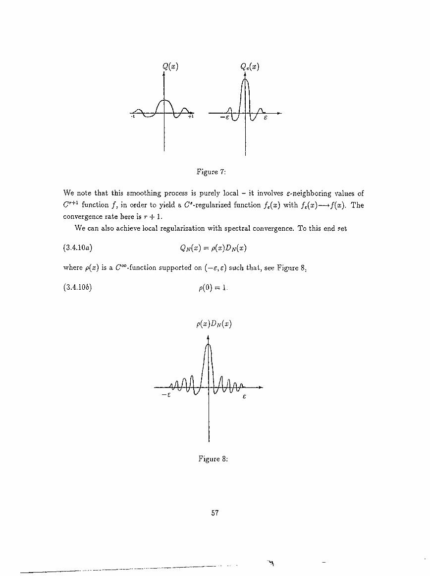
Q(x) Qr(x)

• 1 +1.. -e1

Figure 7:

We note that this smoothing process is purely local - it involves c-neighboring values of

C r +l function f, in order to yield a C--regularized function f,(x) with f,(x)--f(x). The

convergence rate here is r + 1.

We can also achieve local regularization with spectral convergence. To this end set

(3.4.10a) QN(x) = p(x)DN(x)

where p(x) is a Coo-function supported on (-6, e) such that, see Figure 8,

(3.4.10 b) p(O) = 1.

p (x) Div(x)

Figure 8:

57

Consider now:

(3.4.11) fN(x) = QN * f(x).

Then fN(x) is C- because QN is; and the convergence rate is spectral, since by (1.1.25)

f(x) - QN * f(x) = f(x) - lyl< DN(y)p(y)f(x - y)dy

f(x) - p(y)f(x - y)l,=o + residual

where1

(3.4.12b) Iresiduall < Const.I[p(y)f(x - y)[[g,(_ ,C) T for any s > 0.

Thus, the convergence rate is as fast as the local smoothness of f permits; of course with

p =1 we obtain the C'-regularization due to the spectral projection. The role of p was to

localize this process of spectral smoothing.

We can as easily implement such smoothing in the Fourier space: For example, with the

heat kernel we have

(3.4.13) {(k, t) = e-k 2 ,j(k)

so that i(k,t) for any t > 0 decay faster than exponential and hence u(x,t > 0) belong

to H for any s (and by Sobolev imbeddings, therefore, is in C' and in fact analytic). In

general we apply,

00

(3.4.14) f (x) = >1 Q (k)(k)ek

such that for f,(x) to be in H' we require

00

(3.4.15a) E (1 + IkI 2)"IQ (k)J 2(f(k) 2 < Const.

and r 4 1 order of convergence follows with

(3.4.15 b) i(k) - 11 < Const.(Ek)r+l.

Indeed, (3.4.15b) implies00

Jf(x)- f,(x)I < Const. *r+1 Z Ik+lf(k)ekx1

(3.4.16) k-cc

< Const. Maxif(r+l)I• .

58

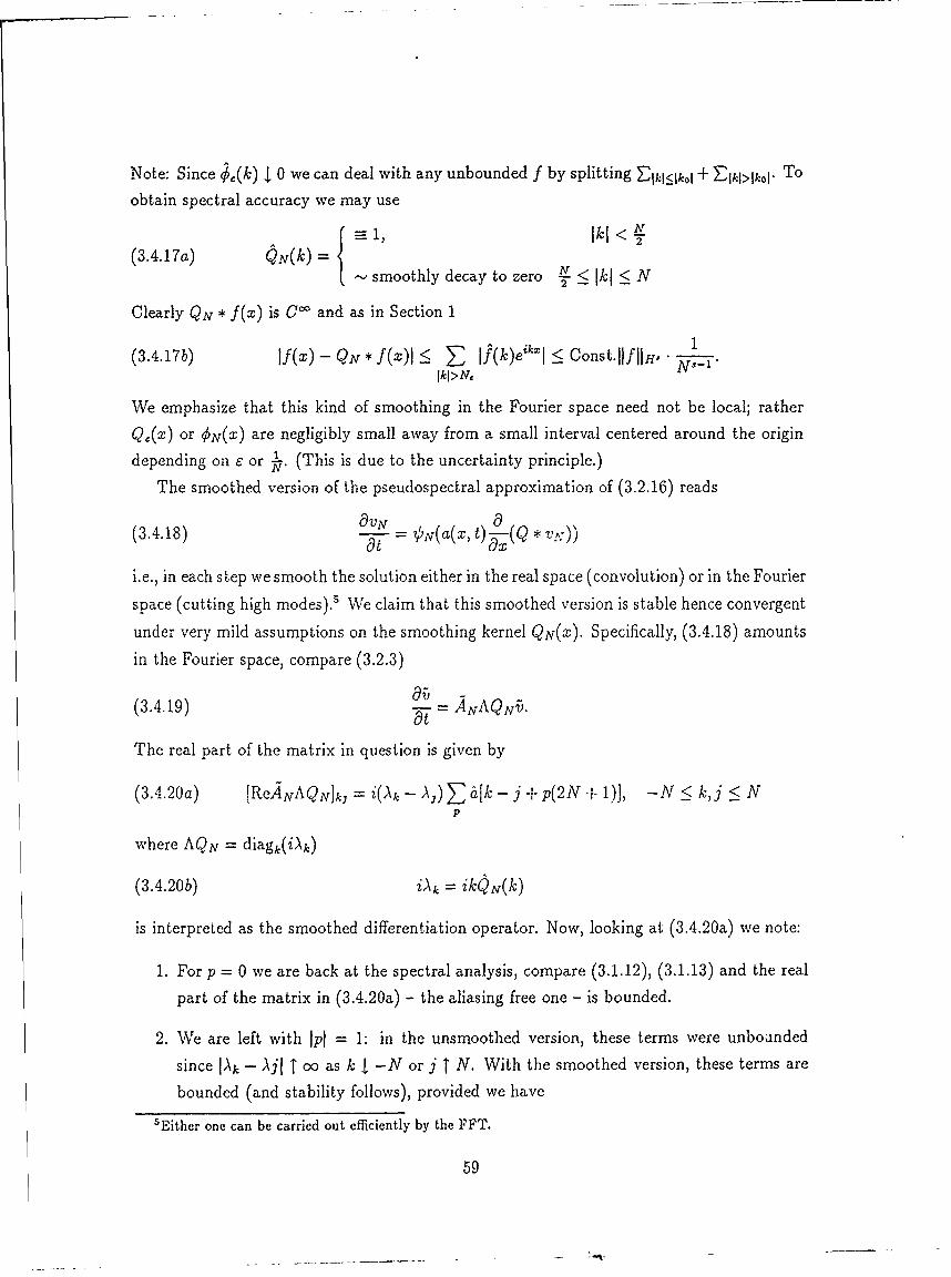
Note: Since q5(k) 1 0 we can deal with any unbounded f by splitting EIk1_<Iko + Z[kj>k1- To

obtain spectral accuracy we may use

= 1 IkI <(3.4.17a) QN(k) = N<[[<N( smoothly decay to zero N -k-

Clearly QN * f(x) is CI and as in Section 1

(3.4.17b) f(x)-QN*f(x)< E If(k)ek, I <Const. IlflH 1Ikl>N,

We emphasize that this kind of smoothing in the Fourier space need not be local; rather

Q,(x) or ObN(x) are negligibly small away from a small interval centered around the origin

depending on e or ,. (This is due to the uncertainty principle.)

The smoothed version of the pseudospectral approximation of (3.2.16) reads

(3.4.18) N= O(a(x, *

i.e., in each step we smooth the solution either in the real space (convolution) or in the Fourier

space (cutting high modes).' We claim that this smoothed version is stable hence convergent

under very mild assumptions on the smoothing kernel QN(x). Specifically, (3.4.18) amounts

in the Fourier space, compare (3.2.3)

(3.4.19) a N

The real part of the matrix in question is given by

(3.4.20a) [ReANAQN]kl = i(Ak -- Aj) Z a[k - j + p(2N + 1)], -N < kj < NP

where AQN = diagk(iAk)

(3.4.20b) iAk = ikQN(k)

is interpreted as the smoothed differentiation operator. Now, looking at (3.4.20a) we note:

1. For p = 0 we are back at the spectral analysis, compare (3.1.12), (3.1.13) and the real

part of the matrix in (3.4.20a) - the aliasing free one - is bounded.

2. We are left with Jpt = 1: in the unsmoothed version, these terms were unbounded

since jAk - AA T co as k I -N or j I N. With the smoothed version, these terms are

bounded (and stability follows), provided we have

5Either one can be carried out efficiently by the FFT.

59

(3.4.21) jAk = ikQN,(k)-- 0IMTN

For example, consider the smoothing kernel QN(x) where(3.4.22a) sin kh h= 27r

Q(k) = kh 2N+ 1,

This yields the smoothed differentiation symbols-- kh

(3.4.22b) Ak = isin -ho.

which corresponds to the second order center differencing in (1.2.36); stability is immediate

by (3.4.21) forsi 2 7rk

2N+1 oklIAkz 10rk

Yet, this kind of smoothing reduces the overall spectral accuracy to a second one; a fourth

order smoothing will be

1 [ .kh 2kh] Ak(3.4.23a) Ak= i 34sinA -sin - , Ivm) = k

or

6i sin kh A,,(3.4.23b) Ak Q nN(k) -

h 4 + 2 cos kh' ikIn general, the accuracy is determined by the low modes while stability has to do with

high ones. To entertain spectral accuracy we may consider smoothing kernels other than

trigonometric polynomials (- finite difference), but rather, compare (3.4.17)--1, kl < N

(3.4.24) QV(k) = 1,-' smoothly decay to zero N < Jkl < N.

2-An increasing portion of the spectrum is differentiated exactly which yields spectral accuracy;

the highest modes are not amplified because of the smoothing effect in this part of the

spectrum.

We close this section noting that if some dissipation is present in the differential model

to begin with, e.g., with the parabolic equation

(3.4.25)- - (a(x' t)au )' a(x,t)cx>0,

then stability follows with no extra smoothing. The parabolic dissipation compensates for

the loss of "one derivative" if first order terms are present. To see this we proceed as follows:

multiply

(3.4.26) O t)= a [ t) OVN t)

60

by VN(xzt) and sum to obtain

(3.4.27) 1 v( ) N OVN

V 19 O

Suppressing excessive indices, VN(xI,, t) v,,(t), we have for the RHS of (3.4.27)

(3--28 V" a,(t) 7 L ~ '9 (a(t)Lv} - Za,(t)

Now, the first sum on the right gives us the usual loss of one derivative and the secondare compensates with gain of such quantity. Petrowski type stability (gain of derivatives)follows. We shall only sketch the details here. Starting with the first term on the right of(3.4.28) we have

I a a/ 19Va 1(3.4.29) T a~v"- ' - I *" + -" [aliasing errors]2aEx\ (ax 2Jax 2

while for the second term

(3.4.30) - a,(t) 2,0 < -a OV' X t) 2d

and this last term dominates the RHS of (3.4.29).

61

APPENDIX

A.1. Fourier Collocation with Even Number of Gridpoints

We assume w(x) is known at

(A.1.1) w, = w(x,) x, =r +vth I,= 0,1,-.. ,2N

with h and 0 < r < h. We use the trapezoidal nodes

1 2N 1 2N-1

(A.1.2) fi(k) = E- > w,e h E wve- kz27r 1,=O -N V=O

to obtain the pseudospectral approximation

N

(A.1.3) IPNW= S "(k)ek .

k=-N

Note: We now have only 2N pieces of discrete data at the different 2N grid points

Xo, X1,'",X2N- and they correspond to 2N waves, as we have a "silent" last mode, i.e.,

with r = 0, k = N, Imle'kx=, = i sin vw = 0. This is a projection, since in view of (A.1.3)

4NW is the interpolant of w(x) at x = x,:

PNW(X)x=. kN [ o 2N I w(x)e-kzj eikx,,

(A.1.4)2N-1 N

E w(x,). 1 S "eNkGI*V)hv=0 k=-N

The aliasing relation in this case reads - compare (1.2.7)00

(A.1.5) i v(k) = E eip2Nriii(k + 2pN)P=- a

and spectral convergence follow - compare with (1.2.16)1

(A.1.6) IIANW(X)IIH. Const, IITNW(X)UjH,, S >

In the usual sin-cos formulation it takes the form

(A.1.7)N [2N[?PNW= 5kcoswabksj)ksin - 1, 0<]k <N.

Nw E "Fk cos kx + 4: sin kx, k N E W(X,,) co

Noting that bN 0 we have 2N free parameters ao, {a k=1 and N to match our data

at {X,120-.

62

NReport Documentation Page

1. Report No. 2. Government Accession No. 3. Recipient's Catalog No.NASA CR-187443

ICASE interim Report 14

4. Title and Subtitle 5 Report Date

SPECTRAL METHODS FOR TIME DEPENDENT PROBLEMS September 1990

6. Performing Organization Code

7 Author(s) 8 Performing Organzation Report No.

Eitan Tadmor Interim Report No. 1410. Work Unit No.

9 Performing Organization Name and Address 505-90-21-01Institute for Computer Applications in Science 11. Contract or Grant No

and EngineeringMail Stop 132C, NASA Langley Research Center NASl-18605Hampton, VA 23665-5225 13 Type of Report and Period Covered

12. Sponsoring Agency Name and Address

National Aeronautics and Space Administration Contractor Report

Langley Research Center 14 Sponsoring Agency Code

Hampton, VA 23665-5225

15 Supplementary Notes

Langley Technical Monitor:Richard W. Barnwell

Interim Report

16 Abstract

This short review on spectral approximations for time-dependent problems con-sists of three parts. In part I we discuss some basic ingredients form the spec-tral Fourier and Chebyshev approximation theory. Part II contains a brief surveyon hyperbolic and parabolic time-dependent problems which are dealt with both theenergymethod and the related Fourier analysis. In part III we combine the ideaspresented in the first two parts, in our study of accuracy stability and conver-gence of the spectral Fourier approximation to time-dependent problems.

17 Key Words (Suggested by Author(s)) -_ 18 Distribution Statement

Fourier approximation, Chebyshev approx- 64 - Numerical Analysisimation, spectral accuracy, hyperbolicand parabolic systems, stability, con-vergence Unclassified - Unlimited

19. Security Classif (of this report) 20 Security Classif. (of this page) 21 No of pages 22. Price

Unclassified Unclassified 68 A04

NASA FORM 1626 OCT 86

NASA-Langey, 1990