open problems in the spectral analysis of evolutionary...

Open Problems in the Spectral Analysis ofEvolutionary Dynamics

Lee AltenbergInformation and Computer Sciences

University of Hawai‘i at Manoa, Honolulu, Hawai‘i U.S.A.∗

[email protected]

Abstract

For broad classes of selection and genetic operators, the dynamics of evolutioncan be completely characterized by the spectra of the operators that define thedynamics, in both infinite and finite populations. These classes include generalizedmutation, frequency-independent selection, uniparental inheritance. Several openquestions exist regarding these spectra:

1. For a given fitness function, what genetic operators and operator intensitiesare optimal for finding the fittest genotype? The concept of rapid first hittingtime, an analog of Sinclair’s “rapidly mixing” Markov chains, is examined.

2. What is the relationship between the spectra of deterministic infinite popu-lation models, and the spectra of the Markov processes derived from them inthe case of finite populations?

3. Karlin proved a fundamental relationship between selection, rates of trans-formation under genetic operators, and the consequent asymptotic mean fit-ness of the population. Developed to analyze the stability of polymorphismsin subdivided populations, the theorem has been applied to unify the reduc-tion principle for self-adaptation, and has other applications as well. Manyother problems could be solved if it were generalized to account for the in-teraction of different genetic operators. Can Karlin’s theorem on operatorintensity be extended to account for mixed genetic operators?

IntroductionA general theory for the performance and design of evolutionary algorithms has provendifficult to achieve. This difficulty sets in even before we delve into search spaces withgreat complexity, or search operators with great complexity. We find it in the simplest

∗Copyright c©2004 by Lee Altenberg. Chapter 4 in Frontiers of Evolutionary Computation, ed. AnilMenon, pp. 73-102. Genetic Algorithms And Evolutionary Computation Series, Vol. 11, Kluwer AcademicPublishers, Boston, MA, 2004. Last corrigenda October 6, 2016.

1

Open Problems in the Spectral Analysis of Evolutionary Dynamics 2

“canonical” models of evolutionary algorithms owing to their nonlinear structure andstochastic dynamics.

Nonlinearity and stochasticity can be eliminated by making a variety of simplifyingassumptions—in essence, exploring a subspace on the boundaries of the general prob-lem. Linearity is produced by assuming constant selection and uniparental transmission(i.e. where the offspring type is determined by the type of its one parent). Determinismcan be produced by assuming an infinite population size. These assumptions producea linear dynamical system whose trajectory and attractors can be described in closedform, and decomposed in terms of its spectrum of eigenvalues and eigenvectors.

Actual evolutionary algorithms depart from this boundary in two important ways:finite populations, and recombination between two (or more) parents.

Recombination, a central innovation of genetic algorithms, is aimed at allowingcombinations of partial solutions to be assembled. Recombination between two parentschanges the dynamics of the infinite population model from linear to quadratic. In aquadratic system, we can no longer obtain a spectrum of eigenvalues and eigenvectors;the methods of nonlinear analysis must be employed, such as characterization of fixedpoints and their stability, domains of attraction, and Lyapunov functions.

A great deal of work has been on the dynamics of recombination and selection formodels at various points on the boundaries of the general problem. A recent com-pendium can be found in Christiansen (2000). For more on quadratic dynamical sys-tems see Rabinovich et al. (1992) and Arora et al. (1994). Progress has been made inthe dynamics of recombination in the absence of selection, in both infinite and finitepopulation models, by Rabani et al. (1995), and for simple selection, by Rabinovichand Wigderson (1999). Numerous analyses for other models on the boundary of thegeneral problem can be found in the evolutionary computation and population geneticsliterature.

Evolutionary algorithms employ finite populations of a size considerably less thanthe cardinality of the search space, since a primary goal of the algorithms is to locatedesired elements of the search space without exhaustive search.

Finite population algorithms typically use Bernoulli sampling to generate new sam-ples of the search space. This changes the model of the algorithm from deterministic tostochastic, a Markov chain which has a linear state transition matrix, but whose dimen-sions are exponentially increased beyond the number of elements in the search space.The first model of finite population dynamics was developed based on Bernoulli sam-pling by Wright (1931) and Fisher (1930). In the Wright-Fisher model, the number ofstates in the Markov chain for the finite population model is O(N |S|), compared to adimension of |S| for the infinite population model, where |S| is the number of differentgenotypes, and N is the population size. Hence, the dimensionality of the state spaceis vastly increased in the finite population model over the infinite population model.

This comparison can be made more concrete by describing the difference in termsof points in the |S| − 1 dimensional simplex. In the infinite population model, the sys-tem state is represented as a single point in the simplex which moves deterministicallyone generation to the next. In the finite population model, the state is represented asa probability distribution over a cloud points in the simplex, restricted to the lattice ofcoordinates {x : N xi ∈ {0, 1, . . . , N},

∑ni=1 xi = 1}. The distribution of the cloud

of points is what changes every generation.


Because the uniparental, infinite population model has a complete solution, in termsof the spectrum of the linear operators, it presents the logical starting point to try to un-derstand a number of unanswered questions in the design and dynamics of evolutionaryalgorithms. So I begin with the uniparental, infinite population modelThere are threeprimary open questions I want to discuss:

1. What are the optimal transmission matrices for finding global optima of a searchspace?

2. What is the relationship between the spectrum of the infinite population modeland the spectrum of the finite population model?

3. Can a key theorem of Karlin on the effects of operator intensity be generalized?

The Canonical ModelThe ‘canonical’ model I shall be referring to throughout is the model of an infinitepopulation evolving with discrete, non-overlapping generations, under constant fitnesscoefficients and generalized uniparental transmission. Let x be the n-dimensional vec-tor of frequencies of different types in the population, so xi ≥ 0, and

∑ni=1 xi = 1,

which is to say that x ∈ ∆n, the n− 1-dimensional simplex. Then the recursion on xis:

x′ =1

wTWx, (1)

where x′ is the vector of frequencies in the next time step; W is the diagonal matrix offitness coefficients, wi ≥ 0;

w =

n∑i=1

wixi

is the mean fitness of the population, used as a normalizer to maintain the system stateas frequencies; and

T =[Tij

]ni,j=1

is the n-by-n matrix of transmission probabilities, Tij , the probability that type j pro-duces an offspring of type i, so

n∑i=1

Tij = 1 ∀j, Tij ≥ 0.

In vector form, these identities are:

1>x = 1, 1>T = 1, and w = 1>Wx,

where

1 =

1...1


The trajectory of the system is:

x(t) =1

ν(t)(TW)t x(0), (2)

where ν(t) = 1>(TW)t x(0) is the normalizer.

1 Optimal Evolutionary Dynamics for OptimizationFor an optimization problem, we assume that an objective function f : S → <+ isdefined on each element of the search space; here, I assume that the goal is to find theelement with maximum objective function value. Exhaustive search or random searchof such a space will require on the average n/2 samples to have sampled an optimumif it is unique (which will be by assumption throughout unless specified otherwise).If an algorithm can find the optimum in an average of εn/2 samples, for some smallconstant ε� 1, then it is clearly doing better than “blind search”.

However, evolutionary algorithms can perform much better thanO(n). The canon-ical example for an “evolutionary algorithm-easy” problem is the ONEMAX problem,where the fitness increases with the number of loci that have 1 as their allelic value(Ackley, 1987). The number of samples required by a simple mutation-selection al-gorithm to find the global optimum in the ONEMAX problem is O(L) = O(log(n)),where L the number of loci, n = |A|L is the size of the search space, A is the set ofalleles for each locus, |A| the cardinality of A (for binary strings, |A| = 2) .

So, as a performance goal, we would like the time complexity our evolutionarysearch to be on the order of the ONEMAX problem, takingO(log(n)) samples in orderto find the global optimum. To be a little more lenient with the performance require-ments, we can relax the condition for “EA-easy” to polylogarithmic time, meaning thatit takes O(P (log(n))) samples to find the optimum, where P (log(n)) is a polynomialin log(n).

So, we wish to know what conditions on an evolutionary algorithm will allow it tofind the global optimum in O(P (log(n))) samples.

Evolutionary algorithms often have multiple domains of attraction (at least in themetastable sense (van Nimwegen et al., 1999)), which imposes a secondary searchproblem: finding the initial conditions that are in the domain of attraction containingthe global optimum. The multiple-attractor problem is usually described as “multi-modality” of the fitness function, but it must be understood that the fitness functionby itself does not determine whether the EA has multiple domains of attraction—it isonly the relationship of the fitness function to the variation-producing operators thatproduces multiple-attractors (Altenberg, 1995).

In order to preclude this secondary search problem, we desire that the algorithmexhibit a single, global attractor that contains the global optimum.

So, we wish to find what spectral properties give rise to the following characteristicsof an evolutionary algorithm:

1. Rapid First Hitting Time: It finds the global optimum using a number of sam-ples that areO(P (log(n))) where n, is the cardinality of the search space. I willcall this the rapid first hitting time property.


2. Global Attraction: It finds the global optimum regardless of the initial samplestaken, i.e. the simplex must have one global attractor containing the optimum.

Search problem that present obstacles to 1. include long path problems, and theneedle-in-a-haystack. Search problem that present obstacles to 2. include deception,rugged adaptive landscapes, and multimodal objective functions.

1.1 Spectral Conditions for Global AttractionFor the canonical model Eq. (1), the global attraction condition, 2. above, can bestated precisely as:

limt→∞

1

ν(t)(TW)t x(0) = π, and π1 > 0, ∀x(0) ∈ ∆n, (3)

where we index the global optimum type as 1, so π1 is its stationary frequency.Condition (3) is guaranteed if and only if T is primitive (irreducible and acyclic),

i.e. there is some v ≥ 0 such that Tv > 0. From the Perron-Frobenius theorem (Gant-macher, 1959), primitiveness guarantees that there be a strictly positive eigenvector πcorresponding to the leading eigenvalue of TW. This eigenvector π, normalized so〈1,π〉 =

∑i πi = 1 , is the global attractor, since the composition of the population

converges to it regardless of the initial composition x(0).Primitiveness in the transmission matrix corresponds to the property of ergodicity.It should be noted that when some types have a fitness of 0, then their frequency

becomes irrelevant to the dynamics, so the transmission probabilities {Tij : j ∈ N},whereN = {i : wi = 0}, are also irrelevant. Hence, primitiveness is required only forthe restriction of T to T+, where

T+ =[Tij

]i,j /∈N

.

For simplicity, I will henceforth assume all fitnesses are positive.It should be noted that ergodicity in the infinite population model gives us little

guarantee that the system in the finite population model will exhibit a global attractor,due to the phenomenon of metastability or broken ergodicity (Palmer, 1982). Whileergodicity in the infinite population model is necessary for ergodicity in the finite pop-ulation model, it is not sufficient. The Markov chain for the finite population modelmust in addition be rapidly mixing (Sinclair, 1992) to avoid broken ergodicity, as willbe discussed later.

1.2 Spectral Conditions for Rapid First Hitting TimesWhat properties of T and W—which here completely define the canonical evolution-ary algorithm—lead to rapid first hitting times? W incorporates the map between theobjective function and the fitness values, wi, and we could certainly focus on the prop-erties of this map. I can pose the following (without belaboring its precise details):

Open Question 1.1. For a given transmission matrix, T, what is the optimum selectionscheme to find the global optimum with a rapid first hitting time?


Here, however, since the canonical model assumes that W is fixed, we wish toconsider the problem for arbitrary W. This leaves only T, the transmission matrix, tobe explored.

We can, without loss of generality, label the unique optimal point in the searchspace with i = 1, so

w1 =n

maxi=1

wi.

We can trivially guarantee a hitting time of 1 by simply constructing a transmissionmatrix that produces the optimum by mutation:

T =

1 1 · · · 10 0 · · · 0...

...0 0 · · · 0

.Transmission in this case is biased to find the optimum without any help from selection.Clearly, such a priori knowledge does not capture the nature of the implicit knowledgethat an evolutionary algorithm must contain to have rapid first hitting times (Altenberg,1995). The essence of evolutionary search is that transmission in the absence of se-lection is unable to produce adaptation or optimization. Only when selection andtransmission are combined does adaptation occur. The translation of this principle intoa condition on T would require that all types evolve to equal frequency in the absenceof selection, i.e.

limt→∞

(T)t x(0) =1

n1, ∀x(0) ∈ ∆n. (4)

Condition (4) for “fair” transmission implies that

1. The transmission matrix is doubly stochastic, i.e. T 1 = 1;

2. The transmission matrix is primitive, i.e. irreducible and acyclic.

So, our question about the optimal characteristics of T can be posed thus:

Open Question 1.2. Given a fitness function on a points in a search space, what “fair”transmission matrix is optimal for finding the global optimum with rapid first hittingtime?

A rapid first hitting time refers to the number of samples that need to be takenbefore finding the global optimum. But in an infinite population, an infinite number ofsamples are taken each generation. So clearly, to adapt the infinite population model tothe problem of rapid first hitting time, we need a proper translation.

In a finite population, with discrete, non-overlapping generations, the number ofsamples, s∗, until the optimum is found is:

s∗ = N τ µ,

where N is the population size, τ is the first hitting time (in generations), and µ isthe fraction of the population each generation that comprise new samples. Hence, to


achieve rapid first hitting times, the population size and the first hitting time itself musteach be polylogarithmic in n = |S|, the size of the search space, sinceO(P (log(n)))∗O(P (log(n))) = O(P (log(n))).

1.3 Rapid Mixing and Rapid First Hitting TimesVitanyi (2000) has investigated the problem of rapid first hitting time in the finite pop-ulation model, and proposes two criteria that will ensure rapid first hitting time:

1. the second-largest eigenvalue of the matrix representing the Markov process isbounded away far enough from 1 so that the Markov chain is rapidly mixing, asdefined by Sinclair (1992).

2. the stationary distribution π gives probability greater than 1/P (log(n)) to the setof states that contain the global optima, where P (log(n)) is a polynomial in thelog of the size of the search space.

The identification of the second-largest eigenvalue as a measure of the speed ofconvergence of the Markov chain in evolutionary dynamics goes all the way back toWright (1931) and Fisher (1930), who solved the second-largest eigenvalue for theMarkov process representing the finite population model. This eigenvalue is λ3 =1− 1/N (since λ1 = λ2 = 1), where N is haplotype population size. It gives the rateof convergence to fixation on a single haplotype due to genetic drift, and is also the rateof decrease in the frequency of heterozygotes in the population. See Ewens (1979, pp.17, 76, 79, 82, 85–90, 105–107, and Appendix B).

Other more recent work investigating the second-largest eigenvalue includes Suzuki(1995), Rudolph (1997), and Schmitt and Rothlauf (2001a,b)

The condition defined by Sinclair (1992) to produce what he calls rapid mixing ina Markov chain is as follows. Sinclair lays out his concept of rapid mixing by firstdefining the relative pointwise distance (r.p.d.) on a Markov process with transitionmatrix P as:

d(t, n) = maxi,j∈{1,...,n}

∣∣∣∣[Pt]ij− πi

∣∣∣∣πi

,

where n is the cardinality of the state space for the chain. Additionally, one defines

τ(ε) = min{t ∈ Z+ : d(t′, n) ≤ ε, ∀t′ ≥ t}.

The Markov chain is said to be rapidly mixing if there exists a polynomialP (log(n), log(1/ε))such that:

maxε∈(0,1]

τ(ε) ≤ P (log(n), log(1/ε))

(Sinclair, 1992, p. 56).Rapid mixing concerns the rate of convergence of a Markov chain to its limiting

probability distribution. The second-largest eigenvalue determines the rate at which thecomponents of the probability distribution that are orthogonal to the limiting distribu-tion die away. The definition of fast optimization which depends on rapid mixing I callrapid first hitting time by analogy.


I propose a slightly different set of criteria from Vitanyi (2000) to allow rapid firsthitting time to be defined in the infinite population model. We can translate the abovediscussion into a condition for rapid first hitting time in the deterministic model thus:

Definition: Rapid First Hitting Time. Consider a deterministic evolutionary algo-rithm with a unique global optimum, which we set to be type 1, so w1 > wi for alli ∈ {2, . . . , n}. Let

τ(ε) = maxx(0)∈∆n

min{t ∈ Z+ : x1(t) ≥ ε}.

The evolutionary algorithm is said to possess a rapid first hitting time if there existpolynomials P1(log(n)) and P2(log(n)) in log(n), such that

ε ≥ 1

P1(log(n))and τ(ε) ≤ P2(log(n))). (5)

For the canonical evolutionary algorithm, x(t) = 1ν(t) (TW)t x(0), this requires

that for all x(0) ∈ ∆n, there exist polynomials P1(log(n)) and P2(log(n)) such that:

x1(P2(log(n))) =1

ν(t)[1 0 · · · 0] (TW)P2(log(n)) x(0) ≥ 1

P1(log(n)). (6)

Of course, it must be emphasized that this ‘translation’ carries with it no presump-tion that the infinite population model adequately approximates the behavior the firsthitting time in the finite population model. The first hitting time is a concept thatproperly belongs to stochastic processes; it is a random variable. The use of the in-finite population model to approximate the first hitting time has been taken before inthe “takeover time” models (Goldberg and Deb, 1991), where a deterministic, infinitepopulation model is used to approximate the time to fixation of a genotype in a finitepopulation. It is clear that this approximation will be inadequate and misleading un-der the very circumstances in which an evolutionary algorithm is of interest, namely,when it can find the fittest elements of the search space by sampling only a fractionof the search space. This circumstances will be discussed in Section 2.1. I claim onlythat this use of the infinite population model may lead us to results that may be worthinvestigating more rigorously in the finite population model.

1.4 Some AnalysisWe can assume without significant loss of generality that TW permits a Jordan canon-ical representation as

TW = W−1/2QΛQ>W1/2, (7)

where the matrix W−1/2Q consists of columns that are the eigenvectors of TW,QQ> = Q>Q = I, and Λ is the diagonal matrix Λii = λi of the eigenvalues ofTW. This assumption will simplify the analysis.


The condition applies if we assume that transition probabilities are symmetric, i.e.Tij = Tji, which is typical of the mutation operators used on data structures in evolu-tionary computation. This is verified by noting that since any symmetric matrix S hasJordan form S = QΛQ>, so we can take S = W1/2 TW1/2 = QΛQ>, hence

TW =(W−1/2Q

)Λ(Q>W1/2

).

We must assume here that all fitnesses are non-zero, wi > 0.With this assumption we can then represent the trajectory in terms of a scaled pop-

ulation vector x(t) := W1/2x′(t) as

x(t) =1

ν(t)QΛtQ>x(0).

We can arbitrarily permute the indices so that λ1 > λ2 ≥ · · · ≥ λn > −λ1, and sothat w1 > w2 ≥ · · · ≥ wn. Then for Qij , i follows the order of the fitnesses, while jfollows the order of the eigenvalues. In particular, with qi being the ith column of Q,

q1 = c π > 0

is the strictly positive leading eigenvector of QΛQ>, with c = 〈1,q1〉 (note that bydefinition 〈qi,qi〉 = 1). Thus:

QΛQ>π = λ1π.

The trajectory of the w1/21 -weighted frequency of the optimal type is:

x1(t) =1

ν(t)

n∑i=1

q1i λti

[q>i x(0)

]=

λt1ν(t)

(q11〈q1,x(0)〉+

n∑i=2

q1i

(λiλ1

)t〈qi,x(0)〉

). (8)

Further evaluation of ν(t) yields:

nν(t) =

n∑i=1

1>qiλtiq>i x(0) (9)

= λt1

[n∑i=1

〈1,qi〉(λiλ1

)t〈qi,x(0)〉

](10)

= λt1

[〈1,q1〉〈q1,x(0)〉+

n∑i=2

〈1,qi〉(λiλ1

)t〈qi,x(0)〉

](11)

= λt1

[c 〈q1,x(0)〉+

n∑i=2

〈1,qi〉(λiλ1

)t〈qi,x(0)〉

], (12)


using c = 〈1,q1〉. So we obtain:

x1(t) =q11〈q1,x(0)〉+

∑ni=2 q1i

(λi

λ1

)t〈qi,x(0)〉

c 〈q1,x(0)〉+∑ni=2〈1,qi〉

(λi

λ1

)t〈qi,x(0)〉

Substituting the above into (6), setting t = P2(log(n)), and rearranging, we obtain thecondition:

[P1(log(n)) q11 − c] 〈q1,x(0)〉 ≥ (13)n∑i=2

(λiλ1

)P2(log(n))

[〈1,qi〉 − P1(log(n)) q1i] 〈qi,x(0)〉

Since q1 = cπ, we substitute P1(log(n)) q11 − c = c [P1(log(n))π1 − 1], and〈q1,x(0)〉 = c〈π,x(0)〉, to get:

c2 [P1(log(n))π1 − 1]〈π,x(0)〉 ≥ (14)n∑i=2

(λiλ1

)P2(log(n))

(〈1,qi〉 − P1(log(n)) q1i) 〈qi,x(0)〉,

∀ x(0) ∈ ∆n.

At this point, we take interest in the second-largest eigenvalue λ2. Let us define

r = λ2/λ1. (15)

For any δ > 0, if r is small enough, then

nδ ≥

∣∣∣∣∣n∑i=2

rP2(log(n)) (〈1,qi〉 − P1(log(n)) q1i) 〈qi,x(0)〉

∣∣∣∣∣ (16)

≥

∣∣∣∣∣n∑i=2

(λiλ1

)P2(log(n))

(〈1,qi〉 − P1(log(n)) q1i) 〈qi,x(0)〉

∣∣∣∣∣ ≥ 0. (17)

In this case, condition (14) is met provided

[P1(log(n))π1 − 1]〈π,x(0)〉 ≥ δ/c2

or

π1 ≥1 + δ

c2 〈π,x(0)〉

P1(log(n))>

1

P1(log(n)). (18)

Hence, for small enough r, the only condition for rapid first hitting time is that thefrequency of the optimum at equilibrium be on the order of P1(log(n))

−1. We knowthat selection is required in order for π1 ≥ 1

P1(log(n)) since the principle eigenvector ofT has π1 = 1

n by the fairness assumption. Thus:


Theorem: 1. If the system x(t) = 1ν(t) (TW)t x(0) exhibits rapid first hitting time,

then there exists a critical value σ∗ ∈ [0, 1) such that the system x(t) = 1ν(t) (TWσ)t x(0)

no longer exhibits rapid first hitting time for all σ ≤ σ∗.

Characterizing the dependence of σ on T and W remains an open question.Now, it remains to be asked, what transmission matrices T minimize r = λ2

λ1?

1.5 Transmission Matrices Minimizing λ2/λ1If we find a transmission matrix that gives r = λ2/λ1 = 0, then the only condition werequire for rapid first hitting time is (18). The rank-1 matrix yields r = 0:

T = U =1

n1 1> =

1

n

1 1 · · · 11 1 · · · 1...

...1 1 · · · 1

.We have λ1(U) = 1, and λ2(U) = · · · = λn(U) = 0. When we include selection:

UW =1

n1 1>W =

1

n1 [w1 w2 · · ·wn] =

1

n

w1 w2 · · · wnw1 w2 · · · wn...

...w1 w2 · · · wn

is also a rank-1 matrix, with eigenvalues λ1(UW) = 1

n

∑ni=1 wi, and λ2(UW) =

· · · = λn(UW) = 0.Thus, it would appear that the rank-1 matrix would be a candidate transmission

matrix to achieve rapid first hitting times. However, this hope is instantly dashed bynoting that for UW, π1 = 1/n, which is not greater than 1/P1(log(n)). We might askif we can find another rank-1 matrix where π1 ≥ 1/P1(log(n)), but this is precluded bythe condition that T be ‘fair’, and thus doubly stochastic, requiring that πi = 1/n for alli. This result is not unexpected, when we consider that the rank-1 matrix correspondsto random search.

So, we are left with the following:

Open Question 1.3. For a given set of fitnesses, W, what classes of fair transmissionmatrices maximize π1 while minimizing r = λ2/λ1 so as to satisfy the conditions forrapid first hitting time?

One step we may take in defining the notion of classes of transmission matrices isto note that the topology of transmission may be separated from the operator intensityby the following parameterization:

T(µ) = (1− µ)I + µ P, (19)

where µ ∈ [0, 1] is the mutation rate, and P is a transmission matrix in which at leastone value Pii = 0 (Altenberg and Feldman, 1987). For those genetic operators that


can be represented as graphs, where a vertex represents a type, and an edge representsan operator transformation from one type to another, then P naturally corresponds to anormalized adjacency matrix for the graph.

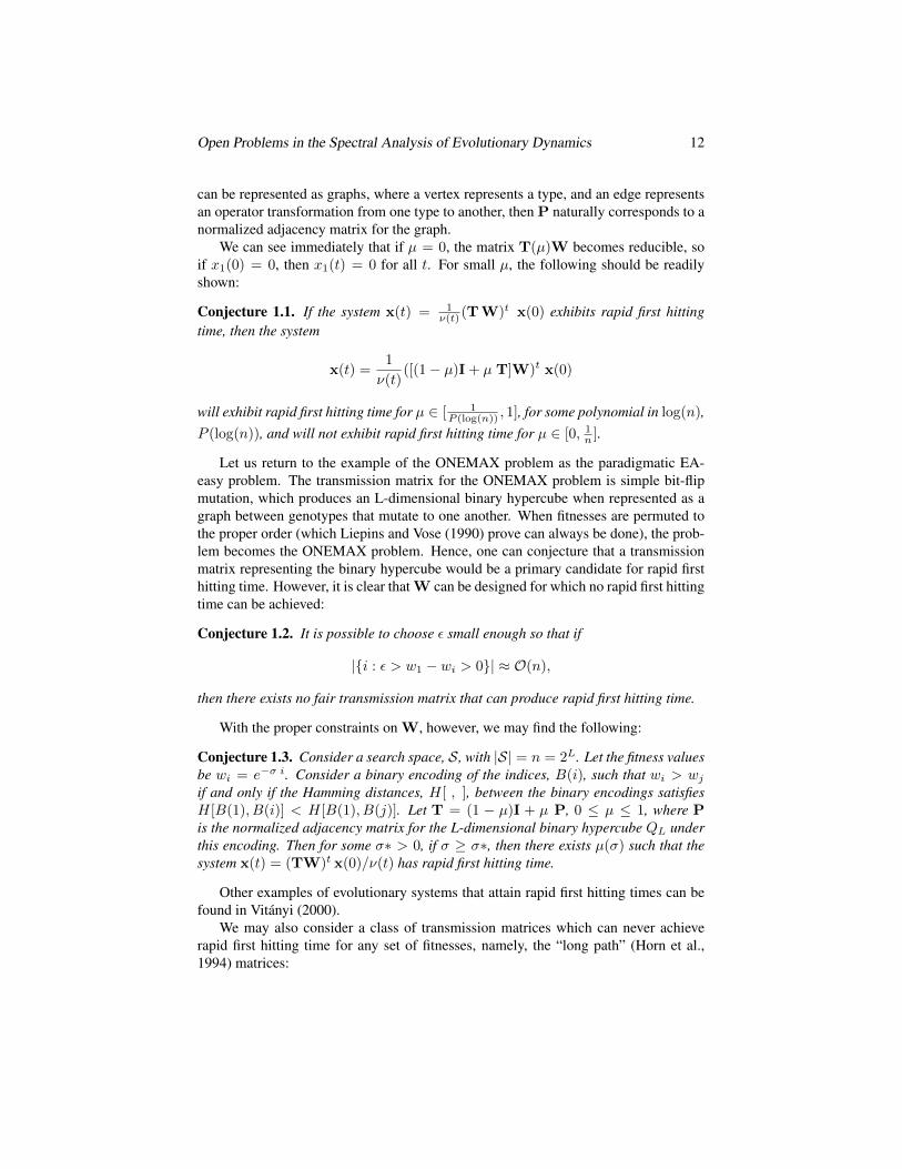
We can see immediately that if µ = 0, the matrix T(µ)W becomes reducible, soif x1(0) = 0, then x1(t) = 0 for all t. For small µ, the following should be readilyshown:

Conjecture 1.1. If the system x(t) = 1ν(t) (T W)t x(0) exhibits rapid first hitting

time, then the system

x(t) =1

ν(t)([(1− µ)I + µ T]W)t x(0)

will exhibit rapid first hitting time for µ ∈ [ 1P (log(n)) , 1], for some polynomial in log(n),

P (log(n)), and will not exhibit rapid first hitting time for µ ∈ [0, 1n ].

Let us return to the example of the ONEMAX problem as the paradigmatic EA-easy problem. The transmission matrix for the ONEMAX problem is simple bit-flipmutation, which produces an L-dimensional binary hypercube when represented as agraph between genotypes that mutate to one another. When fitnesses are permuted tothe proper order (which Liepins and Vose (1990) prove can always be done), the prob-lem becomes the ONEMAX problem. Hence, one can conjecture that a transmissionmatrix representing the binary hypercube would be a primary candidate for rapid firsthitting time. However, it is clear that W can be designed for which no rapid first hittingtime can be achieved:

Conjecture 1.2. It is possible to choose ε small enough so that if

|{i : ε > w1 − wi > 0}| ≈ O(n),

then there exists no fair transmission matrix that can produce rapid first hitting time.

With the proper constraints on W, however, we may find the following:

Conjecture 1.3. Consider a search space, S, with |S| = n = 2L. Let the fitness valuesbe wi = e−σ i. Consider a binary encoding of the indices, B(i), such that wi > wjif and only if the Hamming distances, H[ , ], between the binary encodings satisfiesH[B(1), B(i)] < H[B(1), B(j)]. Let T = (1 − µ)I + µ P, 0 ≤ µ ≤ 1, where Pis the normalized adjacency matrix for the L-dimensional binary hypercube QL underthis encoding. Then for some σ∗ > 0, if σ ≥ σ∗, then there exists µ(σ) such that thesystem x(t) = (TW)t x(0)/ν(t) has rapid first hitting time.

Other examples of evolutionary systems that attain rapid first hitting times can befound in Vitanyi (2000).

We may also consider a class of transmission matrices which can never achieverapid first hitting time for any set of fitnesses, namely, the “long path” (Horn et al.,1994) matrices:


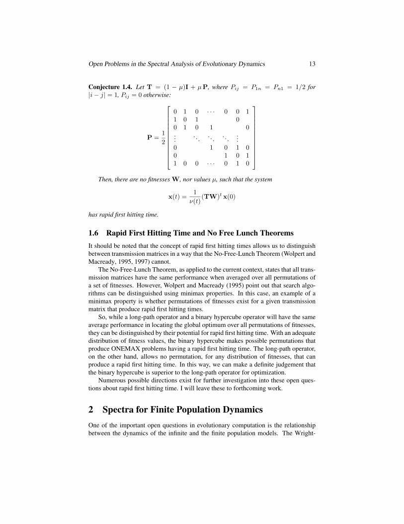
Conjecture 1.4. Let T = (1 − µ)I + µP, where Pij = P1n = Pn1 = 1/2 for|i− j| = 1, Pij = 0 otherwise:

P =1

2

0 1 0 · · · 0 0 11 0 1 00 1 0 1 0...

. . .. . .

. . ....

0 1 0 1 00 1 0 11 0 0 · · · 0 1 0

Then, there are no fitnesses W, nor values µ, such that the system

x(t) =1

ν(t)(TW)t x(0)

has rapid first hitting time.

1.6 Rapid First Hitting Time and No Free Lunch TheoremsIt should be noted that the concept of rapid first hitting times allows us to distinguishbetween transmission matrices in a way that the No-Free-Lunch Theorem (Wolpert andMacready, 1995, 1997) cannot.

The No-Free-Lunch Theorem, as applied to the current context, states that all trans-mission matrices have the same performance when averaged over all permutations ofa set of fitnesses. However, Wolpert and Macready (1995) point out that search algo-rithms can be distinguished using minimax properties. In this case, an example of aminimax property is whether permutations of fitnesses exist for a given transmissionmatrix that produce rapid first hitting times.

So, while a long-path operator and a binary hypercube operator will have the sameaverage performance in locating the global optimum over all permutations of fitnesses,they can be distinguished by their potential for rapid first hitting time. With an adequatedistribution of fitness values, the binary hypercube makes possible permutations thatproduce ONEMAX problems having a rapid first hitting time. The long-path operator,on the other hand, allows no permutation, for any distribution of fitnesses, that canproduce a rapid first hitting time. In this way, we can make a definite judgement thatthe binary hypercube is superior to the long-path operator for optimization.

Numerous possible directions exist for further investigation into these open ques-tions about rapid first hitting time. I will leave these to forthcoming work.

2 Spectra for Finite Population DynamicsOne of the important open questions in evolutionary computation is the relationshipbetween the dynamics of the infinite and the finite population models. The Wright-


Fisher model of finite populations (Wright, 1931; Fisher, 1930)1 is derived from thecanonical model of an infinite population by the addition of only one free parameter—the population size. It thus provides the ideal model in which to pose this question.

2.1 Wright-Fisher Model of Finite PopulationsIn the Wright-Fisher model of a finite population, selection and genetic operators acton the current members of the population to produce a probability distribution fromwhich each member of the population for the next generation is drawn independently.It is as if an infinite zygote pool was created, weighted by selection, from which onlyfinite many can survive, each with equal probability.

The elements of the Wright-Fisher model are mostly the same as for the infinitepopulation model. Let:

N be the population size;

x be the vector of frequencies of each type i in the population, corresponding to N xiindividuals of type i;

x′ be the vector of the frequencies of each type i in the population in the next gener-ation, corresponding to N x′i individuals of type i, produced by taking N inde-pendent samples from the distribution y(x);

y(x) = 1wTWx be the vector representing the probability distribution for drawing an

individual of type i to compose the population in the next generation. T and Wagain represent the transmission matrix and fitness matrix, respectively.

Since the population consists of discrete individuals, the frequency vectors are nowrestricted to a lattice of discrete points on the simplex ∆n, namely

∆n(N) = {x : N xi ∈ {0, 1, . . . , N},n∑i=1

xi = 1}.

The Wright-Fisher model forms a Markov chain, whose transition matrix on frequencyvectors is:

M =[Mx′,x

]x,x′∈∆n(N)

with entries

Mx′,x = N !

n∏i=1

yNx′ii

(Nx′i)!=

N !∏ni=1(Nx′i)!

n∏i=1

(e>i TWx

1>Wx

)Nx′i(20)

where e>i = [0 0 · · · 1 · · · 0 0] has the 1 in the ith position.

1The Markov model by Wright and Fisher is known in the genetic algorithms community as the “Nixand Vose model” (Nix and Vose, 1991). Other work on Markov chains in genetic algorithms includes Gold-berg and Segrest (1987), and (Davis and Principe, 1993), since this community developed largely withoutawareness of prior work in mathematical population genetics.


If we make the assumption that T is primitive, and Tij = Tji, then we may employthe Jordan form (7):

Mx′,x =N !∏n

i=1(Nx′i)!

n∏i=1

(w−1/2i

∑nj=1 qijλj〈qj ,W1/2x〉∑n

j=1 wjxj

)Nx′i. (21)

Wright and Fisher analyzed some simple cases for this Markov system and deriveda number of their properties, including rates of convergence, probabilities of fixation,time to fixation, and stationary distributions of allele frequencies.

In the special case of T = W = I, and n = 2, the solution for all the eigenvaluesof M was found by Feller (1951), and by Cannings (1974) through his method of“exchangeable processes” (see Ewens 1979, pp. 77–79). The solution is:

λ1 = 1 and λi =

i∏j=2

(1− j − 2

N

), i ∈ {2, . . . , N + 1},

where λi refers to the eigenvalues of M, not of TW.Regrettably, the method of exchangeable processes can not be applied when differ-

ent individuals have different offspring probability distributions. We are therefore leftwith the following:

Open Question 2.1. What is the relationship between the eigenvalues and eigenvectorsof TW and those of M?

Since M is defined explicitly in terms of the eigenvalues and eigenvectors of TWin(21), establishing their relationship with the eigenvalues of M is simply a matter ofalgebra. The complexity of the algebra, however, obscures the relationship. One maybe able to simplify the sums in (21) by making assumptions that cause one term todominate the sum, for example, if λ2, · · · , λn = 0. But the utility of such an approachhas yet to be demonstrated.

One can nevertheless make the following observations. Because the state space ofthe system is restricted to the lattice ∆n(N) ⊂ ∆n, and the situation of interest iswhen N ≈ O(log(n)) � n, the vast majority of the entries of any x ∈ ∆n(N) mustbe 0. Thus, ∆n(N) has no points on the interior of ∆n, and is in fact restricted to thelow-dimensional boundaries of ∆n.

Thus, the indices of the non-zero components of x make up a sparse set. Let usdefine the sparse set:

Ψ(x) = {i : xi > 0} (22)

Then we may rewrite (20) as:

Mx′,x =N !∏

i∈Ψ(x′)(Nx′i)!

∏i∈Ψ(x′)

(w−1/2i

∑nj=1 qijλj

∑k∈Ψ(x) qjkw

1/2k xk∑

j∈Ψ(x) wjxj

)Nx′i.

(23)


The trajectory of points in the finite population model will be radically differentfrom the trajectory in the infinite population model. In the finite population model, aprobability distribution will move over the surface of ∆n, while in the infinite popu-lation model, the system will enter the interior of ∆m within v generations, for the vthat gives Tv > 0 and makes T primitive. Evolution in the finite population modelcan be views as transitions between one k-dimensional (k ≤ N ) edge of ∆n andanother, with the probability of transition being highest for types i where the terms∑nj=1 qijλj〈qj ,x〉 are the largest.My earlier discussion of the transmission matrix representing the binary hypercube

took place in the context of the infinite population model. I conjectured that in theinfinite population dynamics it will exhibit rapid first hitting time properties. However,it seems apparent that in the finite population model, the binary hypercube mutationwill be especially advantageous in traversing the low-dimensional boundaries of thesimplex.

I suspect that methods which can analyze (21) as a flow along the low-dimensionalboundaries of the simplex may prove to be most helpful in understanding finite popu-lation dynamics. In the work of van Nimwegen (1999) we find this approach appliedto specific models of mutation and selection, with a nice harvest of analytical results.Answers to the general spectral problem, however, await discovery.

2.2 Rapid First Hitting Time in a Finite PopulationFor a Wright-Fisher model, we can define the criteria for rapid first hitting time in termsof the actual first hitting time for the Markov chain. Here I depart only slightly fromVitanyi (2000).

Let us refer to the set of populations that contain the global optimum as:

B+ = {x ∈ ∆n(N) : x1 > 0},

and conversely, the set of populations that do not contain the global optimum as:

B− = {x ∈ ∆n(N) : x1 = 0},

Suppose that the population always begins fixed on one type other than the optimum,so x(0) = ei, i ∈ {2, . . . , n}.

We cannot use M itself to calculate the probability that the first transition from B−

to B+ occurs at time t, because in calculating[Mt]x+,x−

where x+ ∈ B+ and x− ∈

B−, we can’t know whether this transition is the first transition. However, by setting allthe elements of Mx−,x+ to 0, where x− ∈ B− and x+ ∈ B+, we generate a Markovprocess in which B+ is an absorbing set, hence transition probabilities within B− aftert iterations include the probability that the first hitting time has not yet occurred.

This modified matrix is equivalent to restriction of M to B+, which we shall callM. Then the probability that the global optimum first appears after generation τ is:

Gi(t) =∑

x−∈B−

[M

t]x,ei

= 〈1,Mtei〉


We can define the criteria for rapid first hitting time in terms of the speed at whichGi(τ) declines with τ .

As a basis for comparison, we can consider how Gi(τ) behaves for random search,i.e. M = 1

n1 1>, where n = |∆n(N)|. Then Gi(t) =∑

x−∈B−1n =

(1− 1

n

)Nfor

all i. So

G(τ) =

(1− 1

n

)τN.

In order for G(τ) to be reduced to O(1), to be specific, say G(τ) ≤ 1e , we have:

log[G(τ)] = τN log

(1− 1

n

)≤ −1,

thus for large n, log(1− 1

n

)≈ − 1

n , hence τN ≥ n, which is what we expect. Theessential idea for rapid first hitting time is that we would like τN ≤ P (log(n)). Thethe obvious candidate for a condition to define rapid first hitting time would be:

Definition: Rapid First Hitting Time in a Finite Population. The evolutionary algo-rithm is said to possess a rapid first hitting time if there exist polynomials in log(n),P1(log(n)) and P2(log(n)), such that N ≤ P1(log(n)), and

maxi∈B−〈1,Mτ

ei〉 ≤1

e, for all τ ≥ P2(log(n)), (24)

Clearly, the smaller the spectral radius of M, the more easily that rapid first hittingtime is achieved. We are then ready to pose the main open question regarding thespectrum of evolutionary systems:

Open Question 2.2. What conditions on the eigenvalues and eigenvectors of TWsatisfy condition (24) for rapid first hitting time?

3 Karlin’s Spectral Theorem forGenetic Operator Intensity

Samuel Karlin derived theorem of fundamental significance for evolutionary dynamicsin an article that examines the role of population subdivision in maintaining geneticdiversity (Karlin, 1982). The problem at hand was to understand whether migrationwould enhance or inhibit the maintenance of genetic diversity. Karlin took the ap-proach of finding the conditions that would prevent an allele from becoming extinct,i.e. which would cause it to increase when rare. To this end, he proved a general the-orem on the spectral radius of the stability matrix, which solved his problem for thecase of any number of demes, any migration pattern, and any selection regime—quiteextraordinary in its generality. The theorem is presented below. The square matrix Prepresents the migration pattern, ξ represents the overall migration rate, and the diago-nal matrix W represents the average (or ‘marginal’) selection coefficients of an allelewhen rare.


Theorem: 2 (Karlin, 1982).Let

M(ξ) = (1− ξ)I + ξP,

where P is an irreducible Markov matrix, and let W be a diagonal matrix with strictlypositive diagonal elements, where W 6= aI, for any scalar a. Then the spectral radiusρ(M(ξ)W) is strictly decreasing in ξ:

d

dξρ(M(ξ)W) < 0, for 0 ≤ ξ ≤ 1.

The matrix M(ξ)W represents the stability matrix for the introduction of an alleleinto this multi-deme system. The allele goes extinct when rare if ρ(M(ξ)W) < 1,and is protected from extinction if ρ(M(ξ)W) > 1. Since ρ(M(ξ)W) decreases withξ, the consequence of Karlin’s result is that more migration makes it more difficult tomaintain genetic diversity.

Karlin’s result, obtained to answer a question about migration, proves to have muchdeeper significance for evolutionary dynamics. It reveals a basic property of the relationbetween selection and genetic operators. Its first application outside of the migrationquestion was by Altenberg (Altenberg, 1984; Altenberg and Feldman, 1987) in mod-ifier gene theory. A number of studies in the theory of modifier genes — genes thatcontrol the genetic system, such as rates of mutation (Karlin and McGregor, 1974),recombination (Feldman, 1972; Feldman and Balkau, 1973; Teague, 1976; Feldmanet al., 1980), and migration (Teague, 1977)— all found same result: new alleles whichreduced these rates could always invade a population, suggesting a general “reductionprinciple”. Altenberg (1984) showed that all of these models could be unified witha common representation, M(ξ)W. With this unified representation, the applicationof Karlin’s theorem immediately proves the reduction principle: when an allele thatmodifies rates of mutation, recombination, migration, or any other transformation oftype is introduced into a population near equilibrium, it will increase in frequency if ituniformly reduces the rates of transformation, and go extinct if it uniformly increasesthe rates of transformation.

Another immediate result from Karlin’s theorem regards the mean fitness undera mutation-selection balance. The mean fitness of haploid system decreases with in-creasing mutation rates:

Corollary: 3. Consider an evolutionary system consisting of

• constant selection,

• asexual genetic operators, and

• discrete, non-overlapping generations.

The mean fitness of the population at an attractor is a decreasing function of the prob-ability of the genetic operator acting.

Proof. Let the asexual genetic operator be represented by the Markov matrix M,and let µ is the probability of applying the operator. Then the transmission matrix forthe algorithm is:

T = (1− µ)I + µM,


GENOTYPE

FITNESS

001

000

101

010

011

100

110

111

2 3 4 5 6 7 8

1

2

3

4

5

Figure 1: The Deceptive Trap fitness landscape for three loci with two alleles.

and the recursion for discrete, non-overlapping generations is:

w x ′ = [(1− µ)I + µM] W x

For the global attractor, x, which is the leading eigenvector of TW (whose ex-istence and positive value are established by the Perron-Frobenius Theorem (Gant-macher, 1959)), we have:

[(1− µ)I + µM] W x = T W x = x ρ(TW) = x w.

Hence the mean fitness of the global attractor,

w = ρ( T(µ)W ),

is a decreasing function of the operator probability µ.

3.1 Karlin’s Theorem illustrated with the Deceptive Trap FunctionSuppose a mutation operator is ergodic: i.e. repeated application of the operator canmutate any genotype into any other genotype. Then, under an algorithm of constantselection and mutation, the Perron-Frobenius Theorem shows that there is only onedomain of attraction of the system—i.e. one ‘fitness peak’, as discussed in Section1.1. This may seem contradictory to intuition about ‘multi-modal’ fitness landscapes,in which one would expect multiple domains of attraction. But multiple domains donot occur in haploid, infinite population models under ergodic mutation; finite popu-lations are required to produce quasi-stability of multiple attractors. The global natureof the attractor for ergodic mutation under infinite population size is illustrated withthe Deceptive Trap fitness landscape (Ackley, 1987), shown in Figure 1. In terms ofthe hypercube topology of the graph representing mutation, this is a bimodal fitnessfunction. The frequency vector of the global attractor is shown as a function of themutation rate, for a simple point mutation model, in Figure 2. The mean fitness of theattractor is seen to decrease as a function of the mutation rate, as the Karlin theoremproves. This is shown in Figure 3.


000001

010011

100101

110111

0.25

0.5

0.75

1.

0

0.1

0.2

000001

010011

100101

110GENOTYPE

µ =

OPERATOR INTENSITY

FREQUENCY

Figure 2: There is only one attractor at each value µ, but an ‘error catastrophe’ isevident for µ ≈ 0.5.

0 0.2 0.4 0.6 0.8 13

3.5

4

4.5

5

POPULATIONMEAN

FITNESS

µ = OPERATOR INTENSITY

Figure 3: The mean fitness of the population at the global attractor as a function ofmutation rate. It decreases in accord with Karlin’s theorem.


3.2 Applications for an Extended Karlin TheoremSeveral problems are encountered for which an extended Karlin theorem would allowsolution, but which are currently unsolved. One of these is in modifier theory. Thishas been called ‘self-adaptation’ (Schwefel, 1987; Back, 1996) in the EvolutionaryComputation literature as. In Altenberg (1984) and Altenberg and Feldman (1987) itis proven that the Reduction Principle for linear variation in transmission holds formodifiers that are tightly linked to haplotypes under viability selection (Altenberg andFeldman, 1987, Result 3, p. 565). It is conjectured that the result would also hold forlooser linkage to the modifier locus. The analysis requires that we show for r > 0 thatthe spectral radius of M(µ, r)W decreases in µ, where:

M(µ, r) = (1− µ)[(1− r)I + rQ] + µ[(1− r)S + rS],

with Q, S, and S being Markov matrices (see Altenberg and Feldman (1987) for de-tails). The proof awaits an extension of Karlin’s theorem for r > 0.

The other context of unsolved problems occurs when several transformation pro-cesses act on types in the population, such as the simultaneous action of mutation,recombination, and migration. This can result in recursions of the form:

nwx′ = M(µ, β, γ)Wx (25)= [(1− µ)I + µA][(1− β)I + βB][(1− γ)I + γC]Wx, (26)

where A, B, and C are Markov matrices representing different transformation pro-cesses, and µ, β, and γ are the overall rates of those processes. We wish to know howthe spectral radius of M(µ, β, γ)W changes as a function of each parameter µ, β, andγ. Such a result would allow understanding of genetic recombination can evolve inthe presence of mutation under certain circumstances (Altenberg, 1984; Kondrashov,1988). It is clear that for certain cases of A, B, C, and W, the spectral radius is notmonotonically decreasing in each of µ, β, and γ. However, specifying the conditionsthat produce an increase in the spectral radius with respect to µ, β, γ, etc. requires anextension of Karlin’s theorem. The existence of cases of increase led to the “Principleof Partial Control” for the evolution of genetic modifiers:

Conjecture 3.1. (Altenberg, 1984, p. 149) When a modifier gene has only partial con-trol over the transformations occurring at selected loci, then it is possible for this partof the transformation to evolve an increase.

3.3 Extending Karlin’s TheoremWe need to extend Karlin’s theorem on linear variation from products of the form

[(1− µ)I + µB]W

to products of the more general form

[(1− µ)A + µB]W.


Open Question 3.1. Let

M(µ) = [(1− µ)A + µB],

where A and B are irreducible Markov matrices, and W is a diagonal matrix withstrictly positive diagonal elements not similar to the identity matrix. For what condi-tions on A, B, and W is the spectral radius ρ(M(µ)W) strictly decreasing in µ:

d

dµρ(M(µ)W) < 0, for 0 ≤ µ ≤ 1?

Karlin proved that the spectral radius ρ ([(1− µ)I + µB]W) is decreasing in µ.Clearly each matrix pair {B,W} determines a class of matrices A for which the spec-tral radius ρ ([(1− µ)A + µB]W) is decreasing in µ. Explicit characterization of thisclass is not immediately obvious. However, one can follow Karlin‘s proof to producea condition which would provide the answer if it could be solved.

Suppose that

M(µ, r) = [(1− µ)I + µA][(1− r)I + rB],

where A and B are Markov matrices.I retrace the analysis of Karlin (1982, pp. 195–196). Define

φ(p, µ, r) = supx>0

∑i

pi log

(xi

[M(µ, r)x]i

). (27)

Let x(µ, r) be the vector for which the supremum is attained. The Donsker-Varadhan(1975) variational formula for the spectral radius gives:

log ρ (M(µ, r)D) = supp>0

[〈p, log(D 1)〉 − φ(p, µ, r)] (28)

where D = diag[wi/w

], 1 is the vector of ones, log(v) stands for the vector of

components log(vi),log(D 1) =

[(logwi − logw)

],

and we set∑i pi = 1. Let p(µ, r) be the vector at which this supremum is attained.

Since both x(µ, r) and p(µ, r) as implicitly defined are unique critical points ofφ(p, µ, r),

∂φ(p, µ, r)

∂x(µ, r)=∂φ(p, µ, r)

∂p(µ, r)= 0

for all i. Hence∂ρ

∂µ= −ρ ∂

∂µφ(p, µ, r)

with p = p(µ, r) fixed. Further evaluation paralleling Karlin (1982) yields the condi-tion

∂ρ

∂µ≤ 0 ⇐⇒ (29)

1 ≤∑i

pi(µ, r)[M(0, r)x(µ, r)]i[M(µ, r)x(µ, r)]i

.


For r = 0, Karlin uses Jensen’s inequality to give:

log∑i

pi(µ, 0)xi(µ, 0)

[M(µ, 0)x(µ, 0)]i(30)

≥ φ(p, µ, 0) =∑i

pi(µ, 0) logxi(µ, 0)

[M(µ, 0)x(µ, 0)]i.

By using the principal eigenvector

x = M(µ, 0) x,

the supremum definition of φ gives:

φ(p, µ, 0) ≥∑i

pi(µ, 0) logxi

[M(µ, 0)x]i= 0.

Thus was it is proved that for r = 0, ∂ρ/∂µ ≤ 0. The analysis of (29) for r > 0 doesnot allow us to use (30), and is unsolved. This leaves us with:

Open Question 3.2. What conditions on the matrices A and B, and scalars r and µ,produce

1 ≤∑i

pi(µ, r)[((1− r)I + rB)x(µ, r)]i

[[(1− µ)I + µA][(1− r)I + rB] x(µ, r)]i,

where x(µ, r) and p(µ, r) are the vectors producing the suprema of expressions (27)and (28)?

Another direction to extend Karlin’s theorem, which would be quite relevant to theissue of rapidly mixing Markov chains and rapid first hitting times, is to say somethingabout the second-largest eigenvalue. I would offer (without claiming undue certitude2)the following:

Conjecture 3.2.Let

M(ξ) = (1− ξ)I + ξP,

where P is an irreducible Markov matrix, and let W be a diagonal matrix with strictlypositive diagonal elements not similar to the identity matrix. Then the ratio of thesecond-largest eigenvalue λ2(M(ξ)W), to the spectral radius ρ(M(ξ)W), is strictlyincreasing in ξ:

d

dξ

λ2(M(ξ)W)

ρ(M(ξ)W)> 0, for 0 ≤ ξ ≤ 1.

2October 17, 2005: A counterexample has been provided by Christian Ebenbauer: W =

diag[1, 3, 2

],P =

0.2 0.6 0.20.6 0.1 0.30.2 0.3 0.5

.


3.4 DiscussionKarlin’s theorem, because it holds for arbitrary Markov and fitness matrices, captures afundamental property of Darwinian dynamics, the interaction of selection and transfor-mation caused by genetic operators. What is not generally understood is how multiplegenetic operators interact with one another. Theories that depend on the interactionof recombination, mutation, migration, selection, and drift, such as Wright’s ShiftingBalance Theory (Wright, 1931), pose formidable analytical difficulties. Attempting tounderstand the interaction of multiple genetic operators brings us to the need to extendKarlin’s theorem.

4 ConclusionI hope that the reader, having followed the lines of discussion through this chapter,may come away with the conclusion that the spectra of evolutionary systems providea useful means to pose, and occasionally to solve, problems in evolutionary dynamics.I have used the spectral representation of the generalized mutation-selection systemto address the question of when an evolutionary algorithm is useful for function op-timization. I have described an analog to “rapidly mixing Markov chains” (Sinclair,1992) that is appropriate for optimization, “rapid first hitting time”. The conditionsneeded for an evolutionary algorithm to exhibit rapid first hitting time can be describedin terms of the spectra of the linear systems that, under broad circumstances, can beused to represent them.

I have also posed questions on the dynamics of finite populations in terms of thespectra of the underlying operators. Tying together the spectra of infinite populationmodels with the spectra of the finite population models into which they are embeddedremains a major open question in the theory of evolutionary dynamics. Progress mayresult if flows over the low-dimensional boundaries of the simplex can be modeled.

Lastly, I have reviewed an important theorem by Karlin (1982) on the spectral prop-erties of genetic operator intensity. Extensions of this theorem would find immediateapplication.

Since these are spectral problems, there may indeed already be analytic techniquesthat could be applied to their solution. It is hoped that this chapter may bring attentionto these problems and thus hasten their solution.

5 AcknowledgementsI thank Anil Menon for initiating this book as an outgrowth of the “Hilbert Challenges”for Evolutionary Algorithms session organized for the 2001 International Conferenceon Artificial Intelligence. The open questions on Karlin’s Theorem emerged duringwork on my doctoral dissertation with Marcus W. Feldman and Samuel Karlin in 1983.Early versions of my ideas on rapid first hitting times were vetted in discussions withRichard Palmer and other colleagues while I was a visiting researcher at the Santa FeInstitute in the summer of 1995.


ReferencesAckley, D. H., 1987. A Connectionist Machine for Genetic Hillclimbing, volume

SECS28 of The Kluwer International Series in Engineering and Computer Science.Kluwer Academic Publishers, Boston.

Altenberg, L., 1984. A Generalization of Theory on the Evolution of Modifier Genes.Ph.D. dissertation, Stanford University.

Altenberg, L., 1995. The Schema Theorem and Price’s Theorem. Pages 23–49 inD. Whitley and M. D. Vose, eds. Foundations of Genetic Algorithms 3. MorganKaufmann, San Mateo, CA.

Altenberg, L. and Feldman, M. W. 1987. Selection, generalized transmission, and theevolution of modifier genes. I. The reduction principle. Genetics 117:559–572.

Arora, S., Rabani, Y., and Vazirani, U., 1994. Simulating quadratic dynamical sys-tems is PSPACE-complete. in Proceedings of the 26th Annual ACM Symposiumon Theory of Computing, Pages 459–467. URL citeseer.nj.nec.com/arora94simulating.html.

Back, T., 1996. Evolutionary Algorithms in Theory and Practice: Evolutionary Strate-gies, Evolutionary Programming, Genetic Algorithms. Oxford University Press, Ox-ford.

Cannings, C. 1974. The latent roots of certain Markov chains arising in genetics: Anew approach, I. Haploid models. Advances in Applied Probability 6:260–290.

Christiansen, F. B., 2000. Population Genetics of Multiple Loci. John Wiley and Sons,LTD, Chichester.

Davis, T. E. and Principe, J. C. 1993. A markov chain framework for the simple geneticalgorithm. Evolutionary Computation 1:269–288.

Donsker, M. D. and Varadhan, S. R. S. 1975. On a variational formula for the princi-pal eigenvalue for operators with maximum principle. Proceedings of the NationalAcademy of Sciences U.S.A. 72:780–783.

Ewens, W. J., 1979. Mathematical Population Genetics. Springer-Verlag, Berlin.

Feldman, M. W. 1972. Selection for linkage modification: I. Random mating popula-tions. Theoretical Population Biology 3:324–346.

Feldman, M. W. and Balkau, B. 1973. Selection for linkage modification II. A recom-bination balance for neutral modifiers. Genetics 74:713–726.

Feldman, M. W., Christiansen, F. B., and Brooks, L. D. 1980. Evolution of recombi-nation in a constant environment. Proceedings of the National Academy of SciencesU.S.A. 77:4838–4841.

citeseer.nj.nec.com/arora94simulating.html

citeseer.nj.nec.com/arora94simulating.html


Feller, W., 1951. Diffusion processes in genetics. Pages 227–246 in J. Neyman, ed. Pro-ceedings of the Second Berkeley Symposium on Mathematical Statistics and Proba-bility. University of California Press, Berkeley.

Fisher, R. A., 1930. The Genetical Theory of Natural Selection. Clarendon Press,Oxford.

Gantmacher, F. R., 1959. The Theory of Matrices, volume 2. Chelsea PublishingCompany, New York.

Goldberg, D. E. and Deb, K., 1991. A comparative analysis of selection schemesused in genetic algorithms. Pages 69–93 in G. Rawlins, ed. Foundations of GeneticAlgorithms. Morgan Kaufmann, San Mateo, CA.

Goldberg, D. E. and Segrest, P., 1987. Finite markov chain analysis of genetic algo-rithms. in Proceedings of the Second International Conference on Genetic Algo-rithms, Pages 1–8.

Horn, J., Goldberg, D. E., and Deb, K., 1994. Long path problemsin H. P. Schwefeland R. Manner, eds. Parallel Problem Solving from Nature—PPSN III, volume 866.Springer-Verlag, Berlin.

Karlin, S., 1982. Classifications of selection–migration structures and conditions fora protected polymorphism. Pages 61–204 in M. K. Hecht, B. Wallace, and G. T.Prance, eds. Evolutionary Biology, volume 14. Plenum Publishing Corporation, NewYork.

Karlin, S. and McGregor, J. 1974. Towards a theory of the evolution of modifier genes.Theoretical Population Biology 5:59–103.

Kondrashov, A. S. 1988. Deleterious mutations and the evolution of sexual reproduc-tion. Nature (London) 336:435–440.

Liepins, G. and Vose, M. 1990. Representational issues in genetic optimization. Journalof Experimental and Theoretical Artificial Intelligence 2:101–115.

Nix, A. E. and Vose, M. D. 1991. Modeling genetic algorithms with markov chains.Annals of Mathematics and Artificial Intelligence 5:79–88.

Palmer, R. G. 1982. Broken ergodicity. Advances in Physics 31:669–735.

Rabani, Y., Rabinovich, Y., and Sinclair, A., 1995. A computational view of populationgenetics. in Annual ACM Symposium on the Theory of Computing, Pages 83–92.ISBN 0-89791-718-9. URL citeseer.nj.nec.com/41563.html.

Rabinovich, Y., Sinclair, A., and Wigderson, A., 1992. Quadratic dynamical systems.in IEEE Symposium on Foundations of Computer Science, Pages 304–313. URLciteseer.nj.nec.com/article/rabinovich92quadratic.html.

Rabinovich, Y. and Wigderson, A. 1999. Techniques for bounding the convergencerate of genetic algorithms. Random Structures Algorithms 14:111–138.

citeseer.nj.nec.com/41563.html

citeseer.nj.nec.com/article/rabinovich92quadratic.html


Rudolph, G., 1997. Convergence properties of evolutionary algorithms. Verlag Kovac,Hamburg.

Schmitt, F. and Rothlauf, F., 2001a. On the importance of the second largest eigen-value on the convergence rate of genetic algorithmsin L. Spector, E. D. Goodman,A. Wu, W. B. Langdon, H.-M. Voigt, M. Gen, S. Sen, M. Dorigo, S. Pezeshk, M. H.Garzon, and E. Burke, eds. Proceedings of the Genetic and Evolutionary Compu-tation Conference (GECCO-2001), Pages 559–564. Morgan Kaufmann, San Fran-cisco, California, USA. ISBN 1-55860-774-9. URL citeseer.nj.nec.com/schmitt01importance.html.

Schmitt, F. and Rothlauf, F., 2001b. On the mean of the second largest eigenvalue onthe convergence rate of genetic algorithms. Technical Report Working Paper 1/2001,University of Bayreuth, Department of Information Systems, Universitaetsstrasse30, D-95440 Bayreuth, Germany. Working Papers in Information Systems.

Schwefel, H.-P. 1987. Collective phenomena in evolutionary systems. Preprints ofthe 31st Annual Meeting of the International Society for General System Research,Budapest 2:1025–1033.

Sinclair, A., 1992. Algorithms for Random Generation and Counting: A Markov ChainApproach. Birkhauser, Boston. ISBN 0-8176-3658-7.

Suzuki, J. 1995. A markov chain analysis on simple genetic algorithms. IEE Transac-tions on Systems, Man and Cybernetics 25:655–659.

Teague, R. 1976. A result on the selection of recombination altering mechanisms.Journal of Theoretical Biology 59:25–32.

Teague, R. 1977. A model of migration modification. Theoretical Population Biology12:86–94.

van Nimwegen, E., 1999. The Statistical Dynamics of Epochal Evolution. Ph.D. thesis,Universiteit Utrecht, Amsterdam.

van Nimwegen, E. J., Crutchfield, J. P., and Huynen, M. 1999. Metastable evolution-ary dynamics: Crossing fitness barriers or escaping via neutral paths? Bulletin ofMathematical Biology 62:799–848.

Vitanyi, P. M. B. 2000. A discipline of evolutionary programming. TheoreticalComputer Science 241:3–23. ISSN 0304-3975. URL http://xxx.lanl.gov/abs/cs.NE/9902006.

Wolpert, D. H. and Macready, W. G., 1995. No free lunch theorems for search.Technical Report SFI-TR-95-02-010, Santa Fe Institute, Santa Fe, NM. URLciteseer.nj.nec.com/wolpert95no.html.

Wolpert, D. H. and Macready, W. G. 1997. No free lunch theorems for optimization.IEEE Transactions on Evolutionary Computation 1:67–82.

Wright, S. 1931. Evolution in Mendelian populations. Genetics 16:97–159.

citeseer.nj.nec.com/schmitt01importance.html

citeseer.nj.nec.com/schmitt01importance.html

http://xxx.lanl.gov/abs/cs.NE/9902006

http://xxx.lanl.gov/abs/cs.NE/9902006

citeseer.nj.nec.com/wolpert95no.html

open problems in the spectral analysis of evolutionary...

Documents