1

OBSERVED TIP RESISTANCE AT EOD & BOR USING BOTTOM TIP GAGES FOR DRIVEN PILES

By

YIPENG XIE

A THESIS PRESENTED TO THE GRADUATE SCHOOL OF THE UNIVERSITY OF FLORIDA IN PARTIAL FULFILLMENT

OF THE REQUIREMENTS FOR THE DEGREE OF MASTER OF SCIENCE

UNIVERSITY OF FLORIDA

2011

2

© 2011 Yipeng Xie

3

To my well-beloved professor, Dr. Michael McVay, and to my parents, for their unconditional love

4

ACKNOWLEDGMENTS

I am indebted to my many of my colleagues to support me with this thesis. Most

importantly, I sincerely thank Dr. Michael McVay for serving as my advisor. If I have

ever learned how to do research, or come closer to a geotechnical engineer, it is

because of his great teach by word and deed. There is no doubt that his guidance will

accompany me for the rest of my life. I am impressed by his vast and versatile erudition,

rigorous attitude towards research, and great personality throughout. To be his student

is definitely one of my whole life’s landmarks. His valuable support and encouragement

were what made this possible. Special thanks go to Dr. Reynaldo Roque for sitting on

my supervisory committee. I would also like to thank other fellow graduate students for

making the graduate study an enjoyable experience. A particular word of thanks goes to

Khiem Tran and Jiangpeng Xiang, for unselfishly sharing with me much of their

knowledge.

I would like to thank my parents also, for their self-giving love. Without them, I can

never become who I am today. I hope they will feel proud for me in the future.

5

TABLE OF CONTENTS

page

ACKNOWLEDGMENTS .................................................................................................. 4

LIST OF TABLES ............................................................................................................ 7

LIST OF FIGURES .......................................................................................................... 8

ABSTRACT ................................................................................................................... 11

CHAPTER

1 FOUNDATION INTRODUCTION ............................................................................ 13

1.1 Background of Pile Foundations ....................................................................... 13

1.2 Pile Capacities .................................................................................................. 14 1.2.1 Introduction of Pile Forces ....................................................................... 14 1.2.2 Side Shear Force and Tip Resistance ..................................................... 15

2 PILE SET-UP ( FREEZE ) ...................................................................................... 18

2.1 Introduction to Pile Set-up ( Freeze ) ................................................................ 18

2.2 Principles of Pile Set-up .................................................................................... 19 2.2.1 Observation of Pile Set-up ....................................................................... 19

2.2.2 Findings and Conclusions ....................................................................... 20 2.2.3 Mechanisms of Pile Set-up ...................................................................... 22

2.3 Relationship between Pile Set-up and Logarithm of Time ................................ 24

3 PILE LOAD TESTS ................................................................................................. 28

3.1 Introduction to Pile Load Tests ......................................................................... 28

3.2 Slow and Quick Tests ....................................................................................... 30 3.3 Four Load Test Methods .................................................................................. 30 3.4 Dynamic Forces vs. Static Forces..................................................................... 34

3.4.1 Dynamic Forces Recorded by PDA ......................................................... 34 3.4.2 Match Calculated Forces to Measured Forces With CAPWAP ............... 38

3.4.3 Dynamic Tests Recorded by SmartPile Review ...................................... 40 3.4.4 Wave Theory ........................................................................................... 41

3.4.5 Unloading Point Method ......................................................................... 44

4 ENERGY METHOD ................................................................................................ 47

4.1 Theories of Energy Method ............................................................................... 47 4.1.1 Newton's Three Laws of Motion .............................................................. 47 4.1.2 Force and Energy Equilibrium ................................................................. 48

6

4.1.3 Process of Energy Method ...................................................................... 51 4.1.4 Examples of Energy Method ................................................................... 59

4.1.4.1 Site – Dixie Highway .................................................................... 59

4.1.4.1.1 Compression load test – end bent no.1 ....................................... 59 4.1.4.1.2 Compression load test – Pier no.8 .............................................. 64 4.1.4.2 Site – Caminada Bay ................................................................... 68

5 OBSERVATIONS OF ENERGY APPROACH ........................................................ 72

5.1 EOD vs. BOR Predicted Static Response of Dixie Highway ............................. 72

5.2 EOD vs. BOR Predicted Static Response of Caminida Bay ............................. 74

6 CONCLUSION ........................................................................................................ 88

6.1 Summary .......................................................................................................... 88 6.2 Recommendations ............................................................................................ 89

APPENDIX: EXAMPLES OF ENERGY METHOD ........................................................ 90

LIST OF REFERENCES ............................................................................................. 102

BIOGRAPHICAL SKETCH .......................................................................................... 105

7

LIST OF TABLES

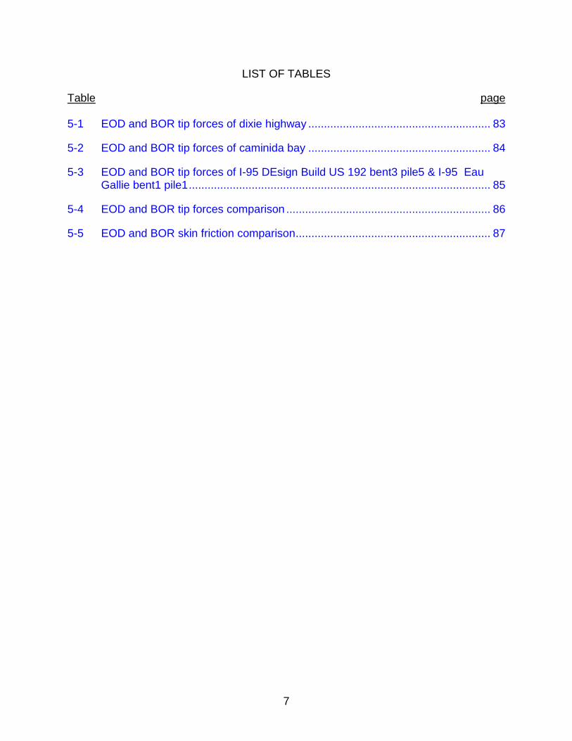
Table page 5-1 EOD and BOR tip forces of dixie highway .......................................................... 83

5-2 EOD and BOR tip forces of caminida bay .......................................................... 84

5-3 EOD and BOR tip forces of I-95 DEsign Build US 192 bent3 pile5 & I-95 Eau Gallie bent1 pile1 ................................................................................................ 85

5-4 EOD and BOR tip forces comparison ................................................................. 86

5-5 EOD and BOR skin friction comparison .............................................................. 87

8

LIST OF FIGURES

Figure page 1-1 Prestressed concrete pile ................................................................................... 14

1-2 Pile total capacity composed of side skin friction and tip resistance ................... 15

1-3 Forces along the pile .......................................................................................... 16

1-4 Forces acting on pile segment during driving ..................................................... 17

2-1 Seidel et at. (1988) relationship between pile capacity and log time ................. 26

3-1 Pile load test frame 1 .......................................................................................... 29

3-2 Pile load test frame 2 .......................................................................................... 29

3-3 Pile instralled with PDA strain gages and accelerometer ................................... 35

3-4 Instrumentation at 18 in from pile tip: PDI (strain and accelerometers). ............. 36

3-5 PDA Data acquisition systems............................................................................ 36

3-6 PDA analyzer ...................................................................................................... 37

3-7 CAPWAP analyze procedure.............................................................................. 40

3-8 EDC software window ........................................................................................ 41

3-9 WaveUp and WaveDown Forces passing along the pile .................................... 41

3-10 Wave traveling in the pile ................................................................................... 41

3-11 Steps of Statnamic test ....................................................................................... 45

3-12 Real field Statnamic test ..................................................................................... 45

3-13 Statnamic measured load and calculated static force ......................................... 46

4-1 Mass-Spring-Damper model ............................................................................... 50

4-2 Excel configuration sheet from SmartPile Review .............................................. 52

4-3 Excel data sheet from SmartPile Review of one blow ........................................ 51

4-4 Excel sheet from Energy Method1 ...................................................................... 53

4-5 Excel sheet from Energy Method2 ...................................................................... 53

9

4-6 EDC Blow 777 Forces vs. Time at Pile Tip of Pier 8 ........................................... 55

4-7 EDC Blow 777 Forces vs. Displacement at Pile Tip of Pier 8 ............................. 56

4-8 EDC Blow 777 Energy vs. Time at Pile Tip of Pier 8 .......................................... 57

4-9 EDC Blow 779 Forces vs. Time at Pile Tip of Pier 8 ........................................... 57

4-10 EDC Blow 779 Forces vs. Displacement at Pile Tip of Pier 8 ............................. 58

4-11 EDC Blow 779 Energy vs. Time at Pile Tip of End Bent1 ................................... 58

4-12 EDC Blow 740 Energy vs. Time at Pile Tip of End Bent1 ................................... 61

4-13 EDC Blow 740 Forces vs. Displacement at Pile Tip of End Bent1...................... 61

4-14 EDC Blow 740 Energy vs. Time at Pile Tip of End Bent1 ................................... 62

4-15 EDC Blow 765 Energy vs. Time at Pile Tip of End Bent1 ................................... 62

4-16 EDC Blow 765 Forces vs. Displacement at Pile Tip of End Bent1...................... 63

4-17 EDC Blow 765 Energy vs. Time at Pile Tip of End Bent1 ................................... 63

4-18 EDC Blow 751 Forces vs. Time at Pile Tip of Pier 8 Pile .................................... 65

4-19 EDC Blow 751 Forces vs. Displacement at Pile Tip of Pier 8 Pile ...................... 66

4-20 EDC Blow 751 Energy vs. Time at Pile Tip of End Bent1 ................................... 66

4-21 EDC Blow 779 Forces vs. Time at Pile Tip of Pier 8 Pile .................................... 67

4-22 EDC Blow 779 Forces vs. Displacement at Pile Tip of Pier 8 ............................. 67

4-23 EDC Blow 779 Energy vs. Time at Pile Tip of Pier 8 .......................................... 68

4-24 EDC Blow 630 Forces vs. Time at Pile Tip of Caminida Bay Bent1 Pile1 ......... 69

4-25 EDC Blow 630 Forces vs. Disp. at Pile Tip of Caminida Bay Bent1 Pile1 ......... 69

4-26 EDC Blow 630 Energy vs. Time at Pile Tip of Caminida Bay Bent1 Pile1 .......... 70

4-27 EDC Blow 660 Forces vs. Disp. at Pile Tip of Caminida Bay Bent1 Pile1 .......... 70

4-28 EDC Blow 660 Energy vs. Time at Pile Tip of Caminida Bay Bent1 Pile1 .......... 71

4-29 EDC Blow 660 Forces vs. Time at Pile Tip of Caminida Bay Bent1 Pile1 .......... 71

5-1 Estimated tip resistance of Dixie Highway Bent 1 Pile1 blows before the load test ...................................................................................................................... 72

10

5-2 Estimated tip resistance of Dixie Highway Bent 1 Pile1 blows after the load test ...................................................................................................................... 72

5-3 Estimated tip resistance of Dixie Highway Pile8 blows before the load test ....... 73

5-4 Estimated tip resistance of Dixie Highway Pile8 blows after the load test .......... 73

5-5 Estimated tip resistance of Caminida Bay1 blows before the load test ............... 74

5-6 Estimated tip resistance of Caminida Bay1 blows after the load test .................. 74

5-7 Estimated tip resistance of Caminida Bay7 blows before the load test ............... 75

5-8 Estimated tip resistance of Caminida Bay7 blows after the load test .................. 75

5-9 Davisson’s Capacity of Dixie Highway Bent1 Pile1 ............................................ 76

5-10 Davisson’s Capacity of Dixie Highway Pier8 ...................................................... 77

5-11 Davisson’s Capacity of Caminida Bay Bent1 ...................................................... 77

5-12 Davisson’s Capacity of Caminida Bay Bent7 ...................................................... 78

5-13 Predicted Tip Resistance at EOD for pile 5 at US 192 ....................................... 80

5-14 Predicted Tip Resistance at BOR for pile 5 at US 192 ....................................... 80

5-15 Predicted Tip Resistance at EOD and BOR for pile 5 at US 192 ........................ 81

5-16 Predicted Tip Resistance at EOD of I95 Eau Gallie bent1 pile1 ......................... 82

5-17 Predicted Tip Resistance at BOR of I95 Eau Gallie bent1 pile1 ......................... 82

5-18 Predicted Tip Resistance at EOD and BOR I95 Eau Gallie bent1 pile1 ............. 83

11

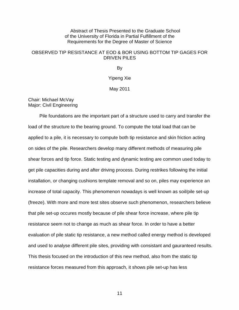
Abstract of Thesis Presented to the Graduate School of the University of Florida in Partial Fulfillment of the Requirements for the Degree of Master of Science

OBSERVED TIP RESISTANCE AT EOD & BOR USING BOTTOM TIP GAGES FOR

DRIVEN PILES

By

Yipeng Xie

May 2011

Chair: Michael McVay Major: Civil Engineering

Pile foundations are the important part of a structure used to carry and transfer the

load of the structure to the bearing ground. To compute the total load that can be

applied to a pile, it is necessary to compute both tip resistance and skin friction acting

on sides of the pile. Researchers develop many different methods of measuring pile

shear forces and tip force. Static testing and dynamic testing are common used today to

get pile capacities during and after driving process. During restrikes following the initial

installation, or changing cushions template removal and so on, piles may experience an

increase of total capacity. This phenomenon nowadays is well known as soil/pile set-up

(freeze). With more and more test sites observe such phenomenon, researchers believe

that pile set-up occures mostly because of pile shear force increase, where pile tip

resistance seem not to change as much as shear force. In order to have a better

evaluation of pile static tip resistance, a new method called energy method is developed

and used to analyse different pile sites, providing with consistant and gauranteed results.

This thesis focused on the introduction of this new method, also from the static tip

resistance forces measured from this approach, it shows pile set-up has less

12

relationship with pile tip force compared to the increase of pile shear force. The current

application of energy method performed on different piles is considered successful.

13

CHAPTER 1 FOUNDATION INTRODUCTION

1.1 Background of Pile Foundations

Pile foundations are important part of a structure used to carry and transfer the

load of the structure to the bearing ground located at some depth below ground surface.

Foundations are generally broken into two categories: shallow foundations and deep

foundations. Shallow foundation is usually, embedded a meter or so into soil. A shallow

foundation is a type of foundation which transfers building loads to the earth very near

the surface, including spread footing foundations, mat-slab foundations, slab-on-grade

foundations, rubble trench foundations, and earthbag foundations. A deep foundation is

a type of foundation distinguished from shallow foundations by the depth they are

embedded into the ground. Structural members made of steel, concrete, and/or timber.

They are expensive due to cost materials, placement (driving, drilling, etc.) vs. shallow

foundations. They are used for following reasons: 1) If the upper soil layers are

compressible or too weak to support the structural loads. 2) Structures subject to large

horizontal forces – In Florida, a common design consideration is hurricane winds, ship

impact on bridge piers, etc. 3) Foundations subject to adverse future influences: soil

erosion or scour from streams or waterways during storms (Acosta 15’ in 25yrs).

Pile foundations have been used as load carrying and load transferring systems

for many years. Two types of forces act on piles, tip resistance acts on the bottom of the

pile and skin friction acts on the sides of the pile. Piles are heavy beams of timber,

concrete, or steel, driven into the earth as a foundation or support for a structure.

Selection of a pile type is based on Cost – in south Florida commercial construction,

auger cast concrete are prevalent – develop more side friction than driven steel or

14

concrete pile due to drilling into limestone (oolites) – resulting in cheaper cost.

Nowadays concrete piles are the most common piles used, which are driven into the

ground to ensure that the foundation is deep. For concrete piles, they are divided into

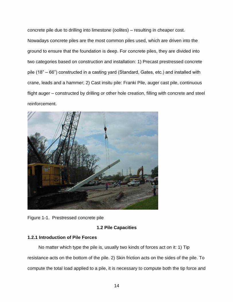
two categories based on construction and installation: 1) Precast prestressed concrete

pile (18” – 66”) constructed in a casting yard (Standard, Gates, etc.) and installed with

crane, leads and a hammer; 2) Cast insitu pile: Franki Pile, auger cast pile, continuous

flight auger – constructed by drilling or other hole creation, filling with concrete and steel

reinforcement.

Figure 1-1. Prestressed concrete pile

1.2 Pile Capacities

1.2.1 Introduction of Pile Forces

No matter which type the pile is, usually two kinds of forces act on it: 1) Tip

resistance acts on the bottom of the pile. 2) Skin friction acts on the sides of the pile. To

compute the total load applied to a pile, it is necessary to compute both the tip force and

15

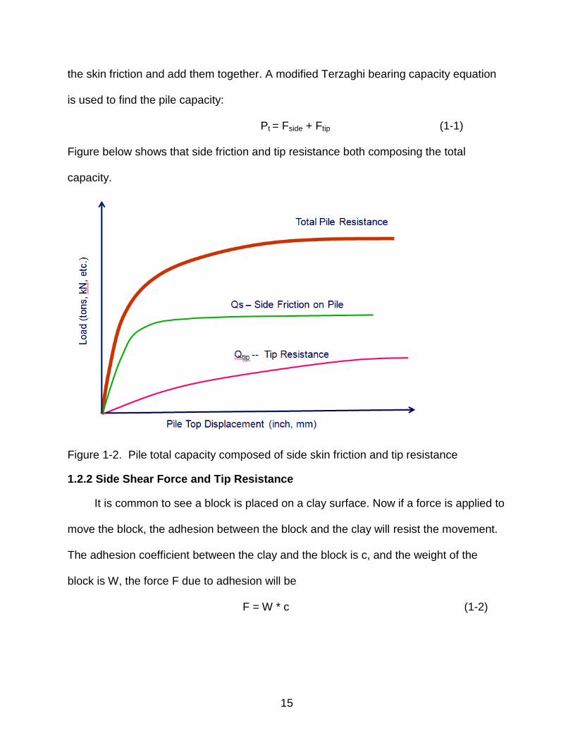
the skin friction and add them together. A modified Terzaghi bearing capacity equation

is used to find the pile capacity:

Pt = Fside + Ftip (1-1)

Figure below shows that side friction and tip resistance both composing the total

capacity.

Figure 1-2. Pile total capacity composed of side skin friction and tip resistance

1.2.2 Side Shear Force and Tip Resistance

It is common to see a block is placed on a clay surface. Now if a force is applied to

move the block, the adhesion between the block and the clay will resist the movement.

The adhesion coefficient between the clay and the block is c, and the weight of the

block is W, the force F due to adhesion will be

F = W * c (1-2)

16

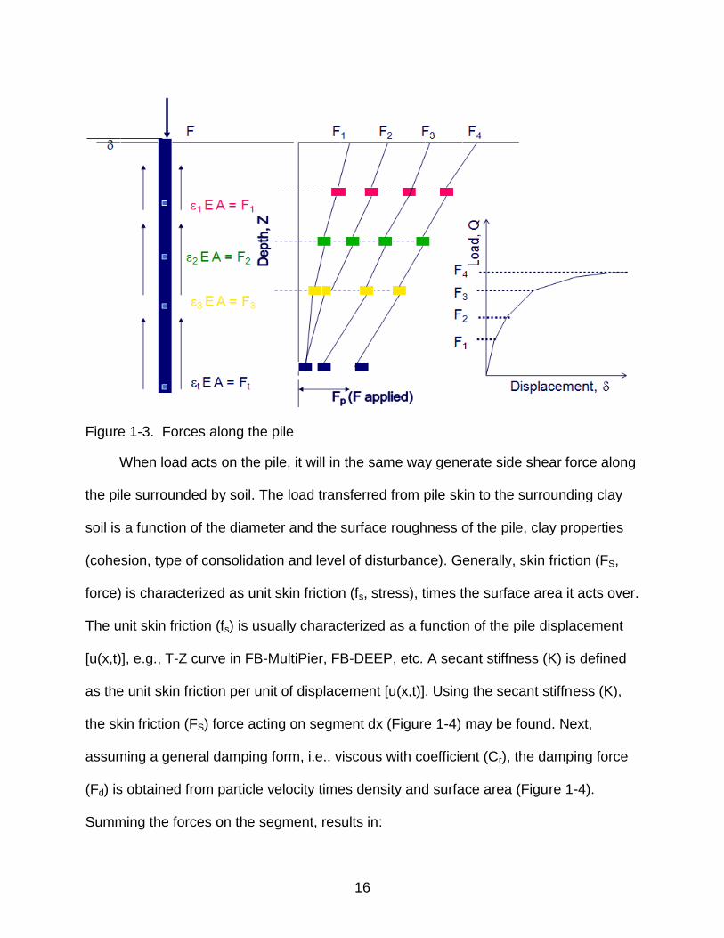
Figure 1-3. Forces along the pile

When load acts on the pile, it will in the same way generate side shear force along

the pile surrounded by soil. The load transferred from pile skin to the surrounding clay

soil is a function of the diameter and the surface roughness of the pile, clay properties

(cohesion, type of consolidation and level of disturbance). Generally, skin friction (FS,

force) is characterized as unit skin friction (fs, stress), times the surface area it acts over.

The unit skin friction (fs) is usually characterized as a function of the pile displacement

[u(x,t)], e.g., T-Z curve in FB-MultiPier, FB-DEEP, etc. A secant stiffness (K) is defined

as the unit skin friction per unit of displacement [u(x,t)]. Using the secant stiffness (K),

the skin friction (FS) force acting on segment dx (Figure 1-4) may be found. Next,

assuming a general damping form, i.e., viscous with coefficient (Cr), the damping force

(Fd) is obtained from particle velocity times density and surface area (Figure 1-4).

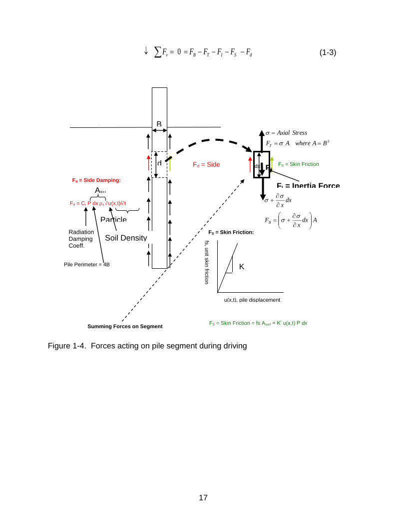
Summing the forces on the segment, results in:

17

(1-3)

Figure 1-4. Forces acting on pile segment during driving

dx

B

dx FI FS = Skin Friction

Fd = Side Damping

FI = Inertia Force

2BAwhereAF

StressAxial

T

Adxx

F

dxx

B

K’

fs, u

nit s

kin

frictio

n

u(x,t), pile displacement

FS = Skin Friction = fs Asurf = K’ u(x,t) P dx

FS = Skin Friction:

Fd = Side Damping:

Fd = Cr P dx s u(x,t)/t

Particle velocity, v

Asu

rf

Radiation Damping Coeff.

Soil Density

Pile Perimeter = 4B

Summing Forces on Segment

dSITBv FFFFFF 0

18

CHAPTER 2 PILE SET-UP ( FREEZE )

2.1 Introduction to Pile Set-up ( Freeze )

For geotechnical engineers, they observed nearly 100 years ago that bearing

capacity of a driven pile usually increases after its installation. During restrikes following

the initial installation, or changing cushions template removal and so on, piles may

experience a driving from easy to hard. This phenomenon nowadays is well known as

soil/pile set-up (freeze). With more installation of driven piles, it is recognized as

occurring in most parts of all the world, all driven pile types, and in all sorts of soils,

which ranges from organic and inorganic saturated clay, and loose to medium dense

silt, sandy silt, silty sand, and fine sand, and is related to both soil and pile properties.

And the timeline is from less than half an hour to several years or even longer. Over

forty years ago, geotechnical engineers observed an averaged 70% pile capacity

increase between 0.5 to 20 days. (Tavenas and Audy (1972)). They wrote the first well-

documented summarization of set-up phenomenon about performing tension load test

on steel pipe piles at sand site in France, claiming the long term set-up was in the

region of 50 to 150% of initial pile capacity. In fact, pile set-up occurs much more quickly

in sand than in clay. Usually, set-up (freeze) takes a few hours for the side-shear friction

to restore in sand, where in clay it may takes months or even years for the piles to

restore total capacity.

Although the phenomenon today is observed more and more and got recognised

in nearly all sorts of soils, the increase capacity of pile with time is not mainly

considered in pile foundation design. It can be imagined that by including the pile set-

up (freeze) into the pile foundation design, the total cost of foundation can be reduced

19

as the number, length, size of the pile could be reduced. It may also generated big

saving in the total cost as foundation cost ranging from 5% to 30% in the total cost.

Although geotechnical engineers realize such advantages as if they can fully use this

phonomenon, but due to lack of understanding about the detailed mechanism, it is hard

to tell how principal factors such as soil type, pile size and material as well as its

installation method affect soil/pile set-up.

2.2 Principles of Pile Set-up

2.2.1 Observation of Pile Set-up

As mentioned before, pile set-up occurs in all kinds of soil. Many papers also

present relating findings. For example:

Bullock et al. (2005) - final research report lasting from February 1993 to April

1999 investigated five fully instrumented piles driven into a variety of soils (sand, clay,

mixed soils) at four different FDOT bridge sites. These five eighteen-inch square piles

were instrumented with strain gages, lateral total stress cells, pore pressure sensors

along their length and at their tips were cast Osterberg load cells. In the field SPT

Torque, piezo CPT and DMT stage testing were performed. Also in laboratory, they

drove a model pile in the centrifuge in flight at 50gs and then perform a static pull out

(tension) test to determine if they could duplicate freeze effects. After 16 to 1727 days

elapsed time using Osterberg cell tests separating side shear and end bearing, 12 to

32% side shear increase per log cycle of time were recorded.

C.S. Chen, S.S. Liew & Y.C. Tan (1998) - two case histories where the changes in

pile capacity were observed with time are presented. One case shows the increase in

pile capacity especially the shaft friction for piles driven into clayey deposit. The average

unit shaft friction, determined from the high strain dynamic pile test, has increased from

20

33 kPa to 57 kPa from 3 days to 33 days after the installation of piles. The second case

shows a tendency of increase in pile capacity for pile driven into sandy deposit over a

period longer than needed for complete dissipation of excess pore water pressure

induced by the driving process.

Gary Axelsson (2000) - two series of full scale field tests were performed on

instrumented concrete piles, driven in loose to medium dense sand. In addition,

laboratory rod shear chamber tests were performed on driven model piles and finally

revealed that set-up is a major feature of driven piles in non-cohesive soil.

Kehoe (1989) - investigated two Florida mixed cohesive soils sites with driven

square prestressed concrete piles. Static and dynamic tests showed capacities

increases average from 58% to 200% within 11 days after driving.

W. K. Ng & M. R. Selamat, K. K. Choong (2010) - based on the assumption that

the capacity increase of pile depends on various factors, the duration of full set-up is

assumed to be dependent solely on soil type, a total 6 case studies (CS) and 11

numbers of test piles (P1 – P11) are presented to investigate from the aspect of soil/pile

set-up. All the projects located in peninsular Malaysia. Two types of pile used in the

cases such as RC square pile (with size 200 – 400mm) and spun pile (with diameter

250 – 500mm), results showing set-up effect is playing a role on time-dependent

capacity of driven pile in Malaysian soil.

2.2.2 Findings and Conclusions

Van E. Komurka and Alan B. Wagner (2003) concluded in their final report

“Estimating Soil/pile Set-up” that through a thorough review of the literature and the

state of the practice, set-up is predominately associated with an increase in soil

resistance acting on the sides (shaft) of a pile. Unit set-up has units of force divided by

21

pile side area. The complete mechanisms contributing to set-up are not well

understood, but the majority of set-up is likely related primarily to dissipation of excess

porewater pressures within, and subsequent remolding and reconsolidation of soil which

is displaced and disturbed as the pile is driven. Set-up is recognized as occurring in

most parts of the world, for virtually all driven pile types, in organic and inorganic

saturated clay, and loose to medium dense silt, sandy silt, silty sand, and fine sand, and

is related to both soil and pile properties. In cohesive soils, the shear strength of the

disturbed and reconsolidated soil has been found to be higher than the soil’s

undisturbed shear strength. In fine-grained granular soils, the majority of set-up is

related to creep-induced breakdown of driving-induced arching mechanisms, and to

aging. The more permeable the soil, the faster set-up develops. Set-up rate decreases

as pile size increases. As soil around and beneath the pile is displaced and disturbed,

excess porewater pressures are generated, decreasing the effective stress of the

affected soil. The increase in porewater pressure is constant with depth (Soderberg,

1961), and can exceed the existing overburden stress within 1 pile diameter of the pile

(Pestana et al., 2002; Randolph, et al., 1979). Decrease in excess porewater pressure

is inversely proportional to the square of the distance from the pile (Pestana et al.,

2002). The time to dissipate excess porewater pressure is proportional to the square of

the horizontal pile dimension (Holloway and Beddard, 1995; Soderberg, 1961), and

inversely proportional to the soil’s horizontal coefficient of consolidation (Soderberg,

1961). Accordingly, larger-diameter piles take longer to set-up than smaller-diameter

piles (Long et al., 1999; Wang and Reese, 1989). Excess porewater pressures dissipate

slower for a pile group than for a single pile (Camp et al., 1993; Camp and Parmar,

22

1999). As excess porewater pressures dissipate, the effective stress of the affected soil

increases, and set-up predominately occurs as a result of increased shear strength and

increased lateral stress against the pile.

Bullock et al. (2005), Axelsson (1998a), and Chow et al. (1998) concluded that

setup occurs primarily as a result of side shear increase, not end bearing. Penetration of

the pile pushes soil outward and away from the pile, destructuring and shearing it to a

greater extent adjacent to the side of the pile than at the pile tip, and thus reducing the

side resistance during installation (and increased aging effects).

2.2.3 Mechanisms of Pile Set-up

Time-dependent pile capacity increase depends on many factors such as soil

grain characteristics, insitu stress level, pile geometry, chemical processes and pile

installation procedure. In cohesionless soil, the excess pore water pressure dissipated

quickly. Excess pore water pressures induced by pile driving seldom exceed 20% of the

effective overburden stress. Soil/pile set-up taking place in pile in cohesionless soil is

thought to be due to the following reasons:

(a) chemical effects which may cause the sand particles to bond to the pile surface,

(b) soil ageing effects resulting in increase in shear strength and stiffness with time,

(c) gain in radial effective stress due to creep effects or relaxation on the established circumferential arching around the pile shaft during installation.

Pile installation in clay is different from pile driving in sand. Komurka et al. divided

the soil/pile set-up mechanisms into the following three phases:

Phase I: logarithmically nonlinear rate of excess pore water pressure

dissipationBecause of the highly disturbed state of the soil, the rate of dissipation of

excess porewater pressures is not constant. During this first phase of set-up, set-up rate

23

corresponds to the rate of dissipation, and so is also not uniform (not linear) with

respect to the log of time for some period after driving. During this phase of non-

constant rate of dissipation of excess pore pressures, the affected soil experiences an

increase in effective and horizontal stress, consolidates, and gains strength in a manner

which is not well-understood and is difficult to model and/or predict. This first phase of

set-up has been demonstrated to account for capacity increases in a matter of minutes

after installation.

Phase II: logarithmically linear rate of excess porewater pressure dissipation

At some time after driving, the rate of excess porewater pressure dissipation

becomes constant (linear) with respect to the log of time. During this second phase of

set-up, set-up rate corresponds to the rate of excess porewater pressure dissipation,

and so for most soils is also constant (linear) with respect to the log of time for some

period after driving. During the logarithmically constant rate of dissipation, the affected

soil experiences an increase in effective vertical and horizontal stress, consolidates, and

gains shear strength according to conventional consolidation theory.

Phase III: Independent of effective stress

Infinite time is required for dissipation of excess porewater pressure to be

complete. Practically speaking, there is a time after which the rate of dissipation is so

slow as to be of no further consequence, at which time it is accepted that primary

consolidation is complete. However, secondary compression continues after primary

consolidation is complete, and is independent of effective stress. Similarly, since the

rate of set-up corresponds to the rate of excess porewater pressure dissipation, it

follows that in some cases infinite time would be required for set-up to be complete.

24

Again practically speaking, and as with primary consolidation, there is likely a time after

which the rate of set-up is so slow as to be of no further consequence, and effective-

stress-related set-up is effectively complete. However, as with secondary compression,

it has been demonstrated that set-up continues after dissipation of excess porewater

pressures. During this third phase of set-up, set-up rate is independent of effective

stress. This is related to the phenomenon of aging.

For a given soil type at a given elevation along the pile shaft, there is likely some

overlap between successive phases, so, more than 1 phase may be contributing to set-

up at a time (e.g., aging may begin before essentially complete dissipation of excess

porewater pressure). In addition, unless soil conditions are uniform along the entire

length of the shaft and beneath the toe, different soils at different elevations will be in

different phases of set-up at a given time.

2.3 Relationship between Pile Set-up and Logarithm of Time

Civil engineers generally assume a log-linear relationship between pile capacity

and elapsed time. Following is Terzaghi’s one dimensional (radial) consolidation theory:

Th = 4* Ch * t / rp2 (2-1)

Where Th = Time Factor Ch = Coefficient of Radial Consolidation t = Elapsed Time since End of Driving rp = pile radius

Based on Terzaghi’s theory, Vesic (1977) found that in clays, pile capacity showed

a linear trend against the logarithm of time except for short and long setup times, which

is similar to a strain vs. log time oedometer consolidation curve. It was raised by them

that due to the dissipation of excess pore pressure as the result of pile installation, set-

up was developed because of the radial consolidation. Researchers further illustrate

25

that the consolidation set-up varies as the square of pile radius, suggesting reduce

some of the variation of Set-up Factors such as pile size would warrant additional

research.

Mohr-Coulomb Equation (2-2) describes side shear increment in the following form:

τ = σ' tan(υ') + c' (2-2)

Where σ' = (σ - u), known as the principle of effective stress. σ is the total stress

applied normal to the shear plane, and u is the pore water pressure acting on the same

plane. υ' = the effective angle of shearing resistance. c' = apparent cohesion, allowing

the soil to possess some shear strength at no confining stress, or even under tensile

stress. It may also be due to diagenetic affects caused by soil aging such as chemical

bonding, cementation of grains and the effects of creep; indeed futher identified that soil

possessed no cohesion when newly remoulded. When shear tests are conducted on an

overconsolidated or dense soil, and peak strengths are plotted on a τ/σ plot, it appears

that cohesion exists as the y-intercept is non-zero. Some feel that this is not due to true

cohesion, but is the effect of interlocking of particles.

From this Mohr-Coulomb equation, some researchers have shown the possibility

which a portion of the set-up is due to the increases in the effective horizontal stress

during consolidation. Experiments demonstrated that at first near the pile the horizontal

effective stresses near the pile are low and increase as time goes by, when the excess

pore water pressure disappears. Also from the experiments done in sand, effective

stress changed from low to high the same with in clay. In conclusion, piles driven both in

clay and sand will have a change in effective stresses, and the increase of horizontal

effective stresses will be a reason for pile set-up effect.

26

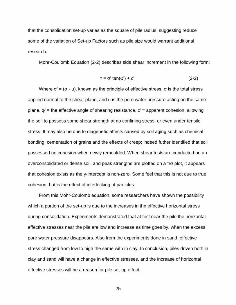
So far, although researchers have not come to a final conclusion of how to predict

the pile set-up exactly and uniformly, it is demonstrated a strong relationship between

pile capacity changes and the logarithm of time.

Figure 2-1. Seidel (1988) ploted relationship between pile capacity and log time

Skov and Denver (1988) reached a relationship between pile capacity and time

from four case histories illustrating set-up, as following:

Q / Q0 – 1 = A * log10 ( T / T0 ) (2-3)

Where Q = pile capacity at time T; Q0 = pile capacity at initial time T0; T = time elapsed since end of driving; T0 = initial time elapsed since end of driving, a reference time before which there is no

predictable Q0 increase as a function of elapsed time.

Skov and Denver (1988) use mostly dynamic tests to reach the A value falling

between 0.2 and 5.0. But for this equation, it is hard to tell the portion of pile side friction

and pile end bearing of the total capacity. As some researches results indicate, pile set-

up occurs primarily due to side shear forces increase instead of pile end bearing. Skov

and Denver, Kehoe and many other researchers found little change with time for pile

27

end bearing from dynamic tests. Also static tests showed such situation from Axelsson’s

research. In Equation 2-3, Q is defined as the total pile capacity which includes the pile

end bearing capacity. Since end bearing may not change a lot, it will cause the set-up

factor lower than the true values. Also further researchers need to concern is the T0.

Because there are no specific criteria to define what time T0 will ends, A will be affected

by it significantly, too. Bullock suggests using T0 = 1 day, so it will give an general

standard criteria for future set-up calculation. Bullock summarized the side shear forces

increase linearly with the log of elapsed time at five test site with different soil situation

in Florida

Bullock et al. (2005) then reviewed all the assumption of set-up factor, further

raised another Set-up factor Ashear as the side shear Semilog-Linear Setup factor to

modify Equation 2-3. He suggests that use T0=1 day to remove the difficulty of finding

the actual start of the semilog-linear set-up process, providing a global reference, also

use Ashear to describe the side shear component only, because end bearing capacity

doesn’t change a lot after end of driving. Finally, plot the EOD capacity at 1 min elapsed

time. It may give a more reliable capacity measurements at fixed times.

Bullock modified Skov and Denver’s equation into set-up factor based on side

shear, providing a more uniformly using equation:

Qs/Qs0=fs/fs0=Ashear * log ( t / t0 )+1 = ( ms / Qs0 ) * log ( t / t0) + 1 (2-4)

Where Ashear = Dimensionless set-up factor; Qs = Side shear capacity at time t; Qs0 = Side shear capacity at initial reference time t0;

fs = Unit side shear capacity at time t; t = Time elapsed since EOD, days; t0 = reference time, recommended to use 1 day; ms = Semilog-linear slope of Qs vs log t

28

CHAPTER 3 PILE LOAD TESTS

3.1 Introduction to Pile Load Tests

Geotechnical engineers find this increase of pile capacity after static load test

(SLT) or dynamic load test (DLT) taken after initial driving. So for determing when pile

set-up (freeze) actually happens or how much influence it affects the total pile bearing

capacity, it is very important that after initial driving, a load test would be conducted

later. Pile foundations are constructed depending on the stiffness of subsurface soil and

ground water conditions with a variety of construction techniques. Due to the extensive

nature of the subsurface mass that it influences, the degree of uncertainty regarding the

actual working capacity of a pile foundation is generally very higher. Load testing is

playing an important role in value engineering and the geotechnical and structural

optimization of foundation solutions. It should be recognized not only in financial terms,

but also with regard to sustainability. Load testing of piles is factored into the project

cost plan and program at an early stage. To perform load tests successfully, it should

allow sufficient time for an objective evaluation of the test results, and subsequent

design revisions engineering to be carried out. A lack of clear objectives and

understanding combined with poorly specified requirements can lead to problems that

could have been avoided such as: 1) insufficient time to carry out tests and to evaluate

the test results; 2) lack of flexibility in the testing regime; 3) no provision for value

engineering; 4) unrealistic performance criteria specified; 5) inappropriate test method

specified; 6) load test conditions are not representative of the working piles; 7) piles

infrequently loaded to failure. It is obvious that continuous improvement in foundation

design and construction practices, while at the same time fulfilling its traditional role of

29

design validation and routine quality control of the piling works can be assured. Data

from pile tests has to be collected and analyzed to enable the piling industry run

smoothly. The test pile, installation equipment and installation procedure should be

identical to that intended to be used for production piles to the extent load. The piles

should be loaded to at least two times the design load, and preferably to failure. Pile

foundations, including helical screw foundations, that have been tested to their ultimate

capacity should not be used as production piles.

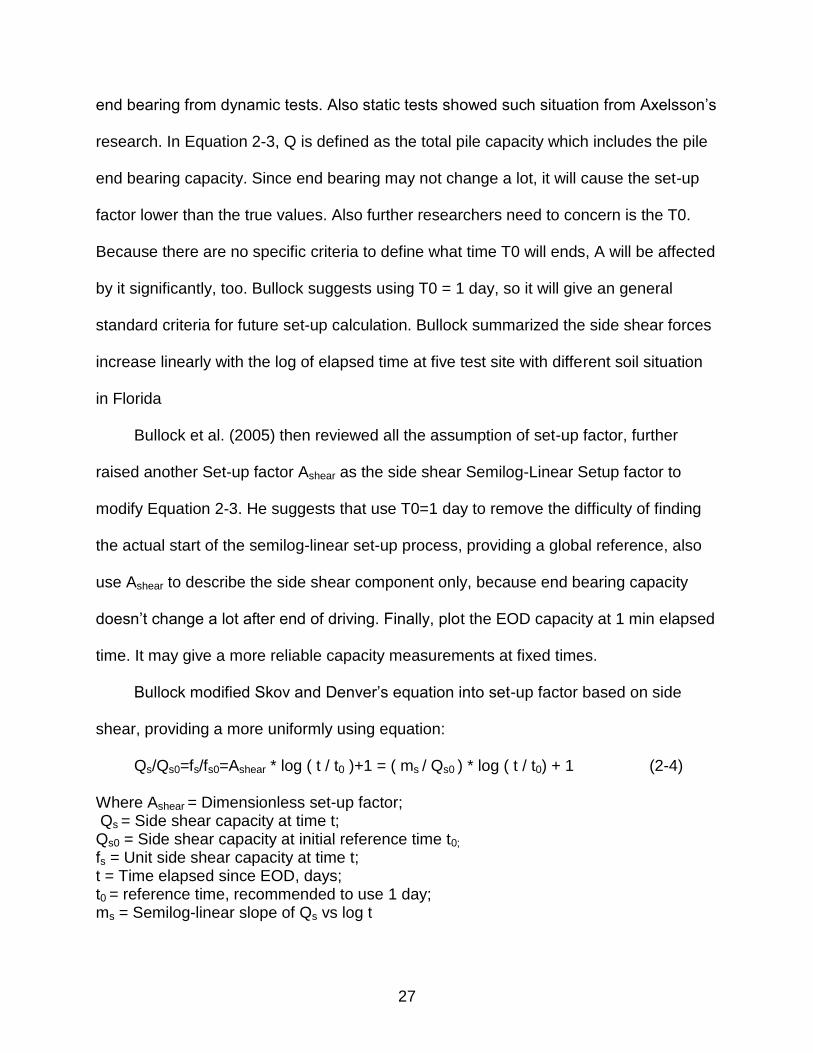
Figure 3-1. Pile load test frame 1

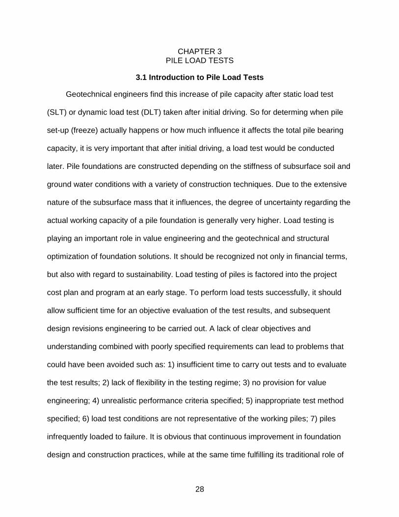
Figure 3-2. Pile load test frame 2

30

3.2 Slow and Quick Tests

Regarding to pile load test, two most common tests are slow and quick maintained

tests (see American Society for Testing and Materials 1143-81).

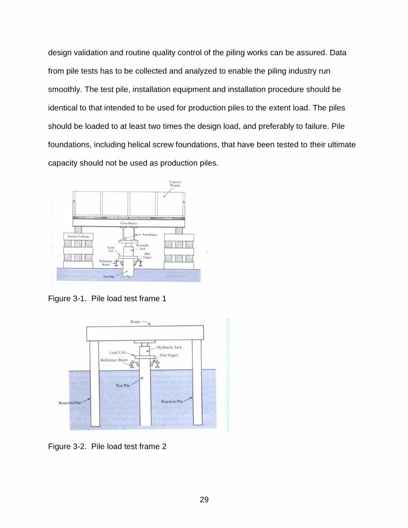
1) Slow Maintained:

– Load the pile in 8 equal increments (25%, 50%, 75%, 100%, 125%, 175% and 200%) of the design service load;

– Maintain each increment until the rate of settlement has decreased to 0.01 in/hour, but not longer than 2 hours;

– Maintain the 200% load for 24 hours;

– After the required holding time, remove the load in decrements of 25% with 1 hour between steps;

– After loading as above, reload pile to test load in 50% increments of design load, allowing 20 minutes between load increments;

– Then increase the load in increments of 10% of design load until failure, allowing 20 minutes between load steps.

2) Quick Maintained – Recommended by Federal Highway Administration (3 – 5 hours):

– Load the pile in 20 increments to 300% of the design load (i.e. each increment is 15% of design load);

– Maintain each load for 5 minutes with readings taken every 2.5 minutes;

– After reaching 300% - hold load for 5 minutes and then remove the load in 4 equal decrements (each 75% of design) with 5 minutes between decrements;

– Because of the quickness of the test, it is not generally recommended for settlement estimations – considered an undrained loading scenario.

3.3 Four Load Test Methods

Dynamic Pile Testing: Dynamic pile testing constitutes a comprehensive and

economical means to quantitatively evaluate the hammer-pile-soil system based on the

measurement of pile force and velocity records under hammer impacts. Measurements,

data processing and analysis are performed in real time in the field by Pile Driving

31

Analyzer® (PDA) equipment from PDITM, or Smartpile ReviewTM which supplies both

top and tip gages. Testing results include estimation of pile load capacity, dynamic pile

stresses and structural integrity as well as driving system performance. The Pile Driving

Analyzer® is applicable on bored cast-in-situ, drilled shafts, continuous flight auger &

driven piles, this applies for either test pile or working pile. Dynamic pile monitoring for

construction quality control and verification testing are performed on hundreds of project

sites in America. Main objectives of dynamic pile testing include obtaining information

on the following: 1) Hammer and driving system performance for productivity and

construction control; 2) Dynamic pile stresses during and after installation. To reduce

the possibility of pile damage, stress must be kept within certain bounds; 3) Pile integrity

during and after installation; 4) Static pile bearing capacity, at the time of testing. For the

evaluation of long term capacity, piles are generally tested during re-strike some time

after installation.

To enhance analysis, CAPWAP® is used combined with PDA, which enables

people to correlate the measured data with the known pile / soil model elements. The

end result of CAPWAP®, via a rigorous and repeated signal matching solution, produces

a pile driving summary that contains pile capacity, percent end bearing / skin friction,

measured pile compression and tension stresses. Using this type of empirical and

analytical data assistance, it can validate a project's design requirements with superior

accuracy and speed. With dynamic load test, researchers want to know:

(a) Estimates total bearing capacity of a pile or shaft (b) Soil resistance parameters (c) Resistance distribution along the shaft and at the toe (d) Static load–settlement curves from the measured force and velocity data (e) Total computed soil capacity – sum of Skin Friction and Toe Bearing (f) Computed load against settlement curve

32

(g)Stresses at any point along the shaft

Static pile load testing: it involves the direct measurement of pile head

displacement in the response to a physically applied test load. It is the most

fundamental form of pile load. Testing has been performed in the load range 100 kN to

12,000 kN. The SLT may be carried out for the following load configurations:

(a) Compression (b) Lateral (c) Tension (i.e. uplift)

For the Static Load Test the load is most commonly applied via a jack acting

against a reaction beam, which is restrained by an anchorage system or by jacking up

against a reaction mass (“kentledge” or dead weight ). The anchorage system may be in

the form of cable anchors or reaction piles installed into the ground to provide tension

resistance. The nominated test load is usually applied in a series of increments in

accordance with the appropriate Code, or with a pre-determined load testing

specification for a project. Each load increment is sustained for a specified time period,

or until the rate of pile movement is less than a nominated value. Static load testing

methods are applicable to all pile types, on land or over water, and may be carried out

on either production piles or sacrificial trial piles. Trial piles are specifically constructed

for the purpose of carrying out load tests and therefore, are commonly loaded to failure.

Testing of production piles however, is limited to prove that a pile will perform

satisfactorily at the serviceability or design load, plus an overload to demonstrate that

the pile has some (nominated) reserve capacity.

Loading is applied to the test pile using a calibrated hydraulic jack, and where

required a calibrated load cell measures the load. During the SLT, direct measurements

33

of pile displacement under the applied loading are taken by reading deflectometers (dial

auges reading to 0.01mm) that are positioned on glass reference plates cemented to

the pile head. The deflectometers are supported by reference beams that are founded a

specified distance away from both the test pile and any reaction points. Although SLT is

generally held as the most reliable form of load testing a pile or pile group, it is important

that interaction effects are minimized. These may result from interaction between the

test pile and the anchorage systems, or between the measuring system and reaction

points. For this reason, careful attention is given to performing the test in accordance

with proper procedures.

Lateral load test: Lateral load test in one of the good means of estimating lateral

capacity of pile. Piles are generally used to transmit vertical and lateral loads to the

surrounding soil media. Piles are sometimes subjected to lateral loads due to wind

pressure, water pressure, earth pressure, earthquakes, etc. when the horizontal

component of the load is small in comparison with the vertical load (say, less than 20%),

it is generally assumed to be carried by vertical piles and no special provision for lateral

load is made. Piles that are used under tall chimneys, towers, high rise buildings, high

retaining walls, bridges & other concrete elevated structures etc. are normally subjected

to high lateral loads. These piles or pile groups should resist not only vertical

movements but also lateral movements. Some of the measured are: 1) Efficiency of the

pile group loads; 2) Soil stiffness degradation; 3) Bending moments 4) Lateral pile

response; 5) Pile deflection and soil response; 6) Ultimate lateral resistance; 7)

Acceptable deflection at working lateral load.

34

Pull-out load test: many structures are constructed using deep piled foundations in

order to transfer structural dead load through unstable ground to a solid stratum. Action

of horizontal wind or wave forces on the structure and the behavior of the piles under

these loads are much less well documented. The resistance of the concrete piles to

pull-out comes from two major sources, skin friction between pile and soil and suctions

generated at the base of the pile as movement occurs. Both of these effects are greatly

affected by the generation of excess or suction pore pressures in the soil due to

movement of the pile. Suctions are generated at the base of the pile in all soils owing to

the opening up of a void as the pile moves. At the sides of the pile, un-drained shearing

of the soil when the pile is pulled quickly will result in excess pore pressure generation

in loose soils and suctions being generated in dense soils. These pore pressures will

alter the effective stress state of the soil and will hence have a great impact on the

force-displacement behavior of the pile. Pull-out tests are the ideal alternative because

of their low cost, relative rapid execution, and reliability of results. The actual skin

resistance between concrete and in-situ soil can be measured at different elevations

within the soil profile. The greater certainty achieved from pullout testing eliminates

overly conservative design values, which in turn reduces as-constructed costs.

Experience has shown that these savings far exceed the cost of pullout testing.

3.4 Dynamic Forces vs. Static Forces

3.4.1 Dynamic Forces Recorded by PDA

Usually performing a static load test after end of driving is a cost of time and

money, needing additional equipment to install loads and measurement of movement

and force. Sometimes pile load test frame’s installation may have some disturb to the

soil. But the estimation of pile tip force is very important for testing pile integrity and

35

prediction of pile performance. Static load test can directly measure pile end bearing

capacity, where provide civil engineers with open-and-shut results. Comparing to taking

long time performing static load tests, people want to measure the static shear forces

and tip resistances more quickly and economically. So getting static results from

dynamic tests is what usually researchers prefer. Since dynamic tests do not disturb soil

around pile during driving and feed back test data simultaneity, it is easy for engineer s

to monitor whether pile driving is smooth or not as well as inspecting pile capacity at the

same time. The need to predict and better understand the ultimate loads to which a

cast-in-place pile foundation is capable is critical for pile design and optimization, as

well as for quality assurance of such elements. The use of high strain dynamic testing of

cast-in-place piles and drilled shafts has become a more frequent routine for bearing

capacity evaluations in many countries around the world, increasing the levels of

standardization and codification (Beim et al. 1998). To accurately predict static capacity

from dynamic pile testing is always being researched by many geotechnical engineers,

and has been the focus of dynamic pile tests on many project sites. Signal matching on

the data seems to be the key of getting more accurately determine capacity.

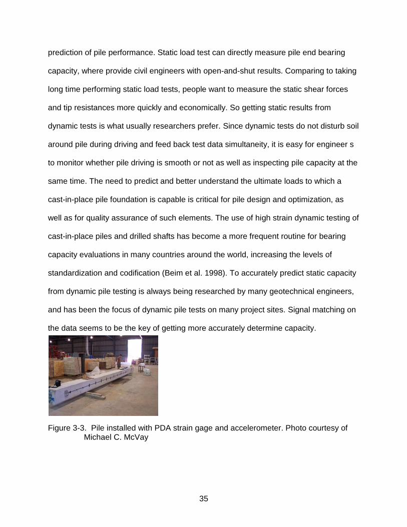
Figure 3-3. Pile installed with PDA strain gage and accelerometer. Photo courtesy of Michael C. McVay

36

Figure 3-4. Instrumentation at 18 in from pile tip: PDI (strain and accelerometers).

Photo courtesy of Michael C. McVay

Figure 3-5. PDA Data Acquisition Systems. Photo courtesy of Michael C. McVay

37

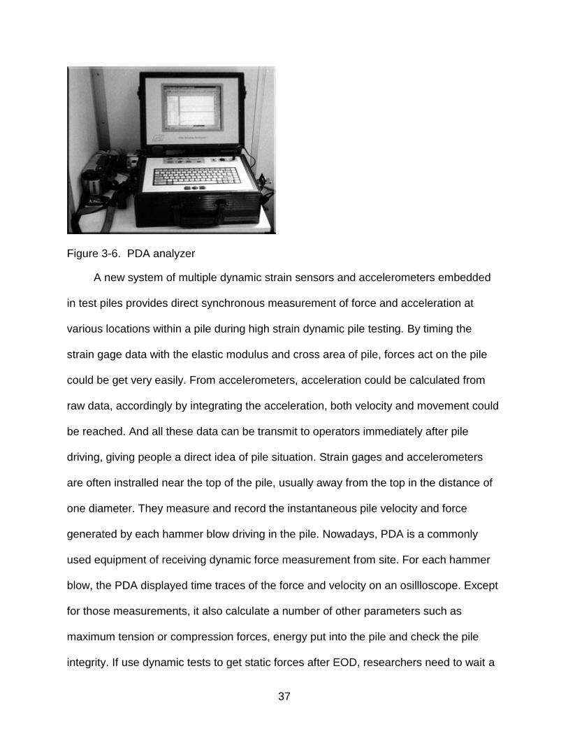
Figure 3-6. PDA analyzer

A new system of multiple dynamic strain sensors and accelerometers embedded

in test piles provides direct synchronous measurement of force and acceleration at

various locations within a pile during high strain dynamic pile testing. By timing the

strain gage data with the elastic modulus and cross area of pile, forces act on the pile

could be get very easily. From accelerometers, acceleration could be calculated from

raw data, accordingly by integrating the acceleration, both velocity and movement could

be reached. And all these data can be transmit to operators immediately after pile

driving, giving people a direct idea of pile situation. Strain gages and accelerometers

are often instralled near the top of the pile, usually away from the top in the distance of

one diameter. They measure and record the instantaneous pile velocity and force

generated by each hammer blow driving in the pile. Nowadays, PDA is a commonly

used equipment of receiving dynamic force measurement from site. For each hammer

blow, the PDA displayed time traces of the force and velocity on an osillloscope. Except

for those measurements, it also calculate a number of other parameters such as

maximum tension or compression forces, energy put into the pile and check the pile

integrity. If use dynamic tests to get static forces after EOD, researchers need to wait a

38

similar time as performing static load test, waiting until pore water pressure dissipates

and pile set-up increases.

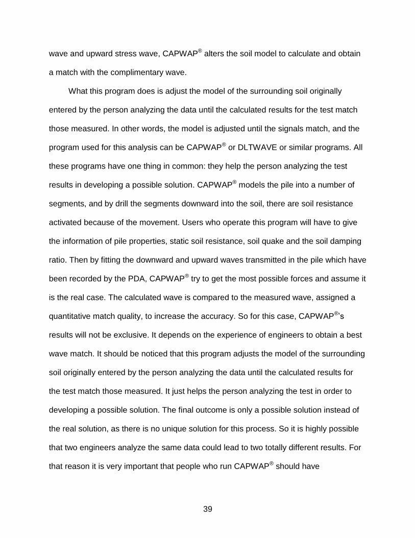
3.4.2 Match Calculated Forces to Measured Forces With CAPWAP

After PDA collects raw data from test field, recorded force and velocity waves from

selected hammer blows will be analyzed using the CAPWAP® computer program to

separate the skin friction and tip resistance from the total force. CAPWAP® (CAse Pile

Wave Analysis Program) is a software program that estimates total bearing capacity of

a pile or shaft, as well as resistance distribution along the shaft and at the toe. The

program takes as input the force and velocity data obtained with a Pile Driving

Analyzer® (PDA). This instrumentation system creates an opportunity to explore side

and end bearing pile resistance distribution with confidence and reliability than from top

measurements alone. Because PDA measures the dynamic forces during pile driving, it

is difficult to know exactly how much the static force is. Along with the popularization of

CAPWAP®, it is considered a standard procedure for the capacity evaluation from high

strain dynamic pile testing data. CAPWAP® separates static and damping soil

characteristics and also allows for an estimation of the side shear distribution and the

pile’s end bearing. CAPWAP® is based on the wave equation model, which analyses

the pile as a series of elastic segments and the soil as a series of elasto-plastic

elements with damping characteristics, where the stiffness represents the static soil

resistance and the damping represents the dynamic soil resistance. Typically the pile

top force and velocity measurements acquired under high strain hammer impacts can

be analyzed utilizing the signal matching procedure yielding forces and velocities over

time and along the pile length. Using one pile top measurement which is easy to install

and protected during pile driving from damage, recording both the downward stress

39

wave and upward stress wave, CAPWAP® alters the soil model to calculate and obtain

a match with the complimentary wave.

What this program does is adjust the model of the surrounding soil originally

entered by the person analyzing the data until the calculated results for the test match

those measured. In other words, the model is adjusted until the signals match, and the

program used for this analysis can be CAPWAP® or DLTWAVE or similar programs. All

these programs have one thing in common: they help the person analyzing the test

results in developing a possible solution. CAPWAP® models the pile into a number of

segments, and by drill the segments downward into the soil, there are soil resistance

activated because of the movement. Users who operate this program will have to give

the information of pile properties, static soil resistance, soil quake and the soil damping

ratio. Then by fitting the downward and upward waves transmitted in the pile which have

been recorded by the PDA, CAPWAP® try to get the most possible forces and assume it

is the real case. The calculated wave is compared to the measured wave, assigned a

quantitative match quality, to increase the accuracy. So for this case, CAPWAP®’s

results will not be exclusive. It depends on the experience of engineers to obtain a best

wave match. It should be noticed that this program adjusts the model of the surrounding

soil originally entered by the person analyzing the data until the calculated results for

the test match those measured. It just helps the person analyzing the test in order to

developing a possible solution. The final outcome is only a possible solution instead of

the real solution, as there is no unique solution for this process. So it is highly possible

that two engineers analyze the same data could lead to two totally different results. For

that reason it is very important that people who run CAPWAP® should have

40

experience.

Figure 3-7. CAPWAP® analyze procedure

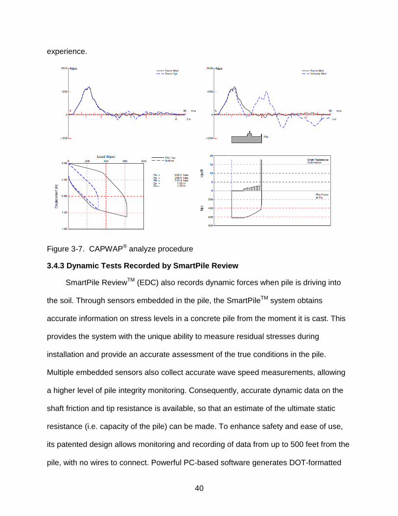
3.4.3 Dynamic Tests Recorded by SmartPile Review

SmartPile ReviewTM (EDC) also records dynamic forces when pile is driving into

the soil. Through sensors embedded in the pile, the SmartPileTM system obtains

accurate information on stress levels in a concrete pile from the moment it is cast. This

provides the system with the unique ability to measure residual stresses during

installation and provide an accurate assessment of the true conditions in the pile.

Multiple embedded sensors also collect accurate wave speed measurements, allowing

a higher level of pile integrity monitoring. Consequently, accurate dynamic data on the

shaft friction and tip resistance is available, so that an estimate of the ultimate static

resistance (i.e. capacity of the pile) can be made. To enhance safety and ease of use,

its patented design allows monitoring and recording of data from up to 500 feet from the

pile, with no wires to connect. Powerful PC‐based software generates DOT‐formatted

41

reports, provides multi‐user access with password control, and allows data review from

both current as well as past projects.

Figure 3-8. EDC software window

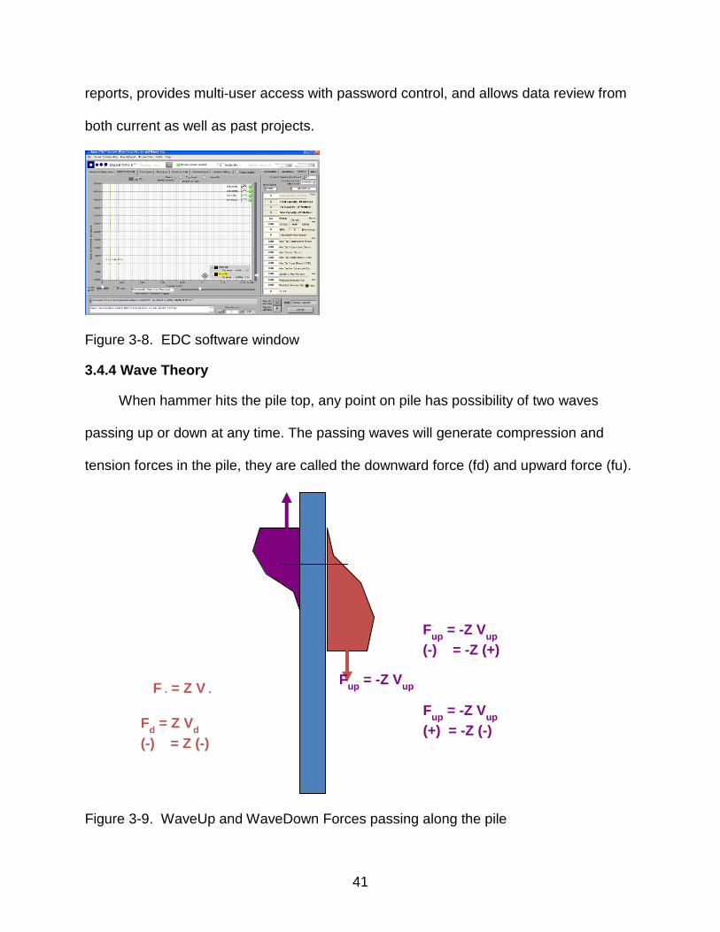
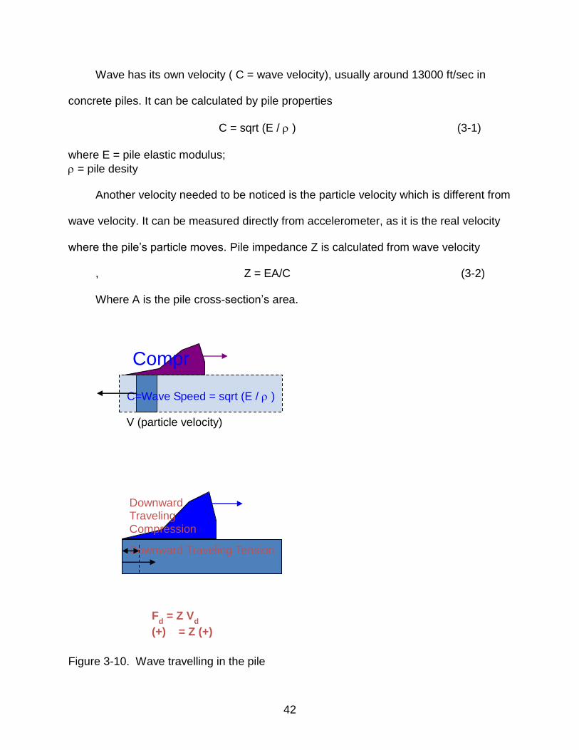
3.4.4 Wave Theory

When hammer hits the pile top, any point on pile has possibility of two waves

passing up or down at any time. The passing waves will generate compression and

tension forces in the pile, they are called the downward force (fd) and upward force (fu).

Figure 3-9. WaveUp and WaveDown Forces passing along the pile

Fd = Z V

down

Fup

= -Z Vup

(-) = -Z (+)

Fup

= -Z Vup

Fup

= -Z Vup

(+) = -Z (-) F

d = Z V

d

(-) = Z (-)

42

Wave has its own velocity ( C = wave velocity), usually around 13000 ft/sec in

concrete piles. It can be calculated by pile properties

C = sqrt (E / ) (3-1)

where E = pile elastic modulus;

= pile desity

Another velocity needed to be noticed is the particle velocity which is different from

wave velocity. It can be measured directly from accelerometer, as it is the real velocity

where the pile’s particle moves. Pile impedance Z is calculated from wave velocity

, Z = EA/C (3-2)

Where A is the pile cross-section’s area.

Figure 3-10. Wave travelling in the pile

Compression Wave

V (particle velocity)

C=Wave Speed = sqrt (E / )

Downward Traveling Tension

Downward Traveling Compression

Fd = Z V

d

(+) = Z (+)

43

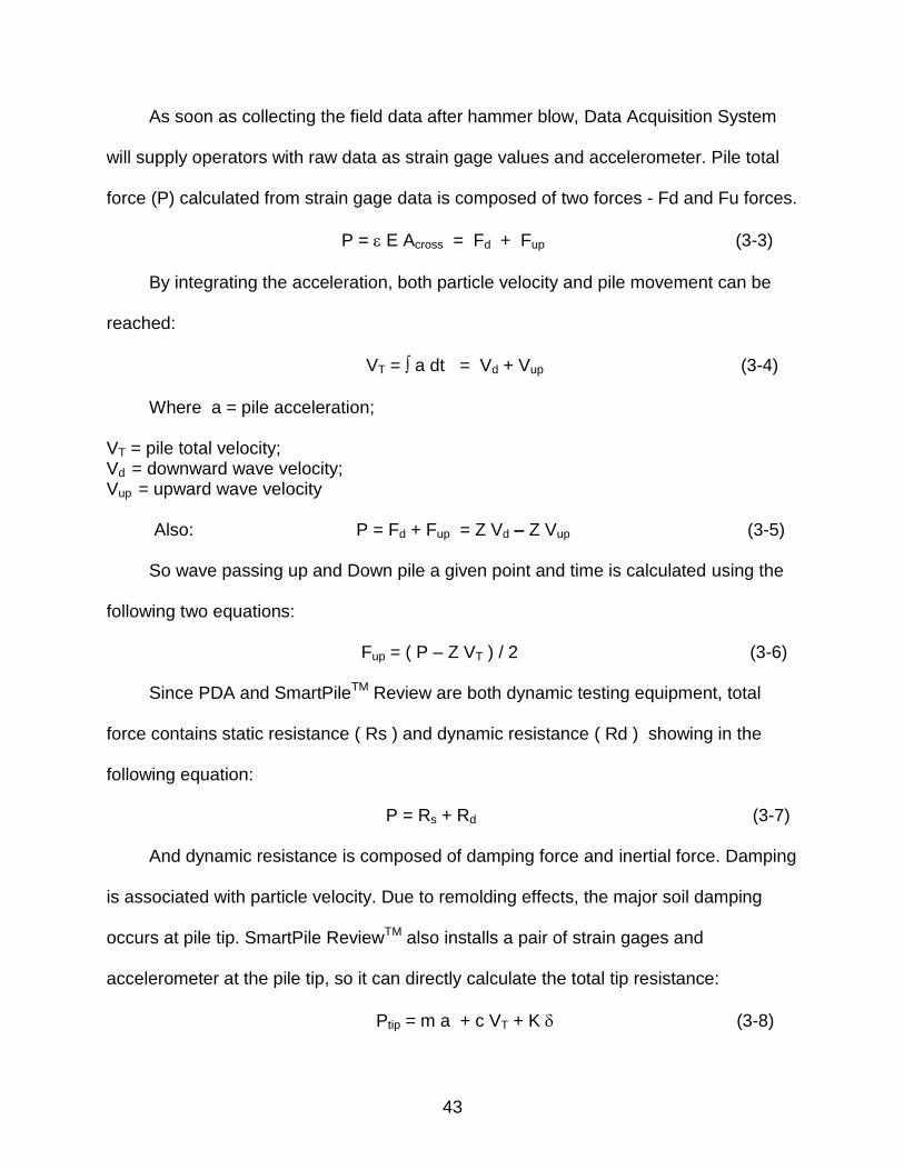
As soon as collecting the field data after hammer blow, Data Acquisition System

will supply operators with raw data as strain gage values and accelerometer. Pile total

force (P) calculated from strain gage data is composed of two forces - Fd and Fu forces.

P = E Across = Fd + Fup (3-3)

By integrating the acceleration, both particle velocity and pile movement can be

reached:

VT = a dt = Vd + Vup (3-4)

Where a = pile acceleration;

VT = pile total velocity; Vd = downward wave velocity; Vup = upward wave velocity

Also: P = Fd + Fup = Z Vd – Z Vup (3-5)

So wave passing up and Down pile a given point and time is calculated using the

following two equations:

Fup = ( P – Z VT ) / 2 (3-6)

Since PDA and SmartPileTM Review are both dynamic testing equipment, total

force contains static resistance ( Rs ) and dynamic resistance ( Rd ) showing in the

following equation:

P = Rs + Rd (3-7)

And dynamic resistance is composed of damping force and inertial force. Damping

is associated with particle velocity. Due to remolding effects, the major soil damping

occurs at pile tip. SmartPile ReviewTM also installs a pair of strain gages and

accelerometer at the pile tip, so it can directly calculate the total tip resistance:

Ptip = m a + c VT + K (3-8)

44

Where Ptip = the total tip force measured from tip strain gage;

M = pile tip mass; a = tip acceleration measured from tip accelerometer; c = damping ratio; K = pile tip stiffness;

= pile tip movement, also measured from tip accelerometer. 3.4.5 Unloading Point Method

Full-scale testing can be an integral component of quality control/quality assurance

for projects involving construction of deep foundations. Rapid load tests are being used

in the deep foundation industry as a method for assessing the axial static behavior of

deep foundations. Since rapid load tests involve dynamics, inertial and damping forces

must be considered in analyzing measured pile response to estimate the static pile

response.

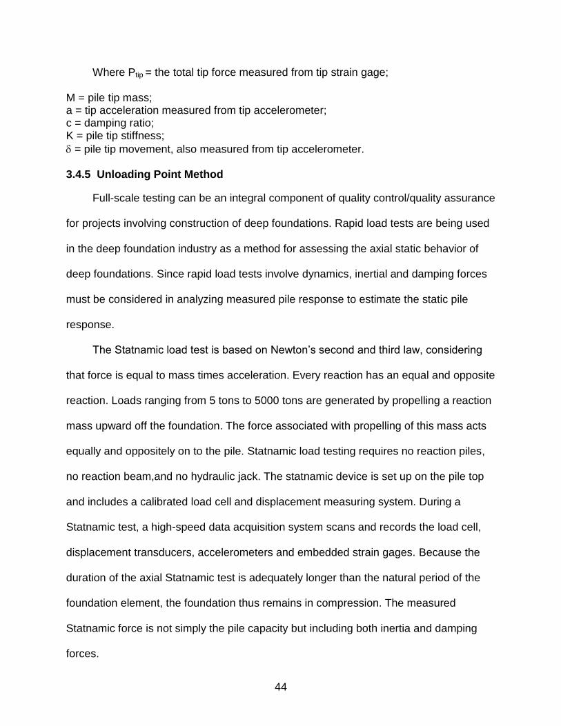
The Statnamic load test is based on Newton’s second and third law, considering

that force is equal to mass times acceleration. Every reaction has an equal and opposite

reaction. Loads ranging from 5 tons to 5000 tons are generated by propelling a reaction

mass upward off the foundation. The force associated with propelling of this mass acts

equally and oppositely on to the pile. Statnamic load testing requires no reaction piles,

no reaction beam,and no hydraulic jack. The statnamic device is set up on the pile top

and includes a calibrated load cell and displacement measuring system. During a

Statnamic test, a high-speed data acquisition system scans and records the load cell,

displacement transducers, accelerometers and embedded strain gages. Because the

duration of the axial Statnamic test is adequately longer than the natural period of the

foundation element, the foundation thus remains in compression. The measured

Statnamic force is not simply the pile capacity but including both inertia and damping

forces.

45

Figure 3-11. Steps of Statnamic Test

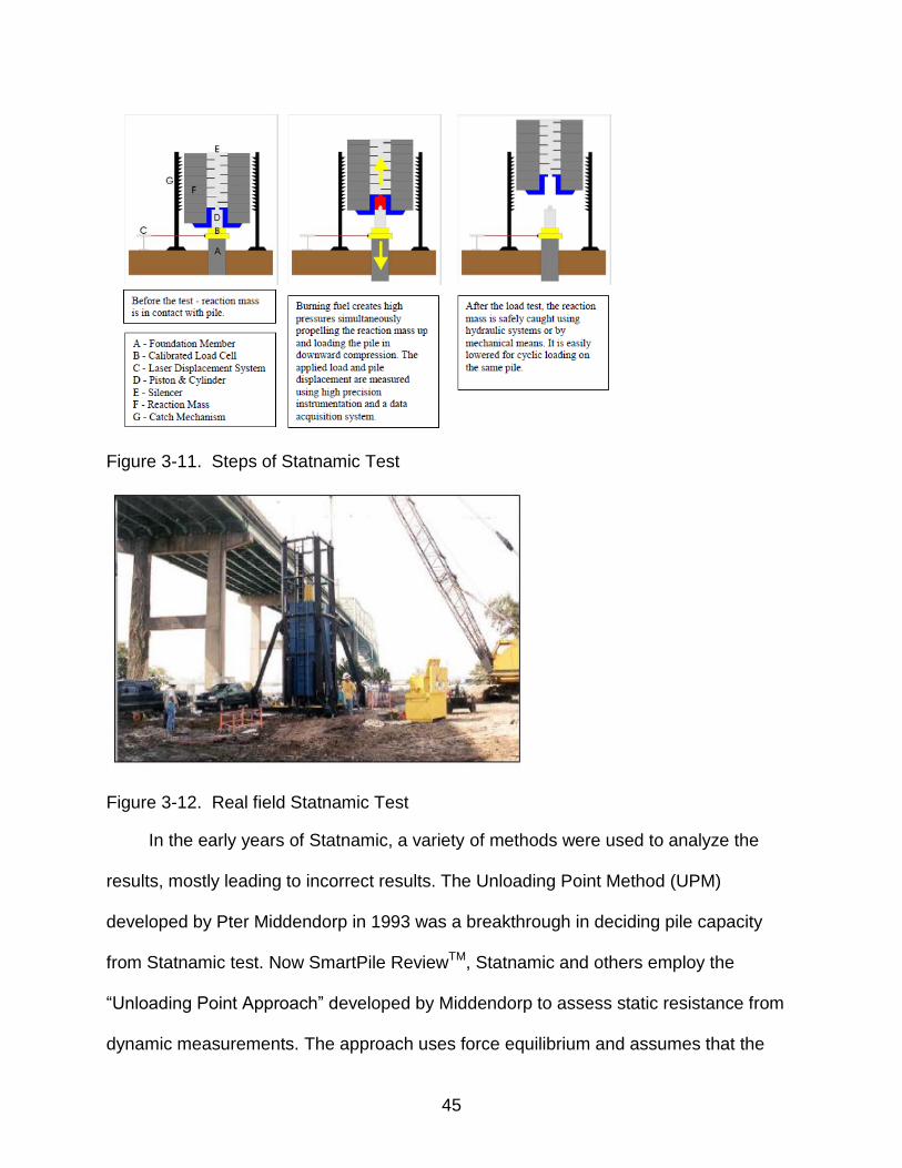
Figure 3-12. Real field Statnamic Test

In the early years of Statnamic, a variety of methods were used to analyze the

results, mostly leading to incorrect results. The Unloading Point Method (UPM)

developed by Pter Middendorp in 1993 was a breakthrough in deciding pile capacity

from Statnamic test. Now SmartPile ReviewTM, Statnamic and others employ the

“Unloading Point Approach” developed by Middendorp to assess static resistance from

dynamic measurements. The approach uses force equilibrium and assumes that the

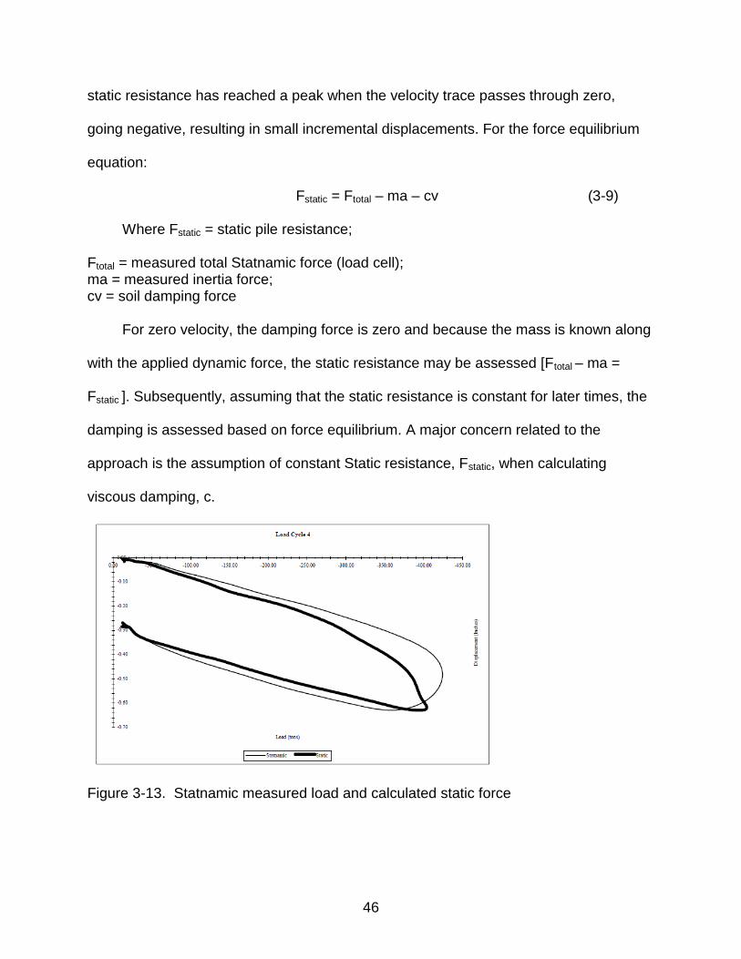
46

static resistance has reached a peak when the velocity trace passes through zero,

going negative, resulting in small incremental displacements. For the force equilibrium

equation:

Fstatic = Ftotal – ma – cv (3-9)

Where Fstatic = static pile resistance;

Ftotal = measured total Statnamic force (load cell); ma = measured inertia force; cv = soil damping force

For zero velocity, the damping force is zero and because the mass is known along

with the applied dynamic force, the static resistance may be assessed [Ftotal – ma =

Fstatic ]. Subsequently, assuming that the static resistance is constant for later times, the

damping is assessed based on force equilibrium. A major concern related to the

approach is the assumption of constant Static resistance, Fstatic, when calculating

viscous damping, c.

Figure 3-13. Statnamic measured load and calculated static force

47

CHAPTER 4 ENERGY METHOD

4.1 Theories of Energy Method

4.1.1 Newton's Three Laws of Motion

Before introducing energy method implemented in pile tip for accessing tip static

resistance, it’s better to review Newton's Three Laws first which is the core of this brand

new approach. They are three physical laws that form the basis for classical mechanics.

They describe the relationship between the forces acting on a body and its motion due

to those forces. They have been expressed in several different ways over nearly three

centuries, and can be summarized as follows:

(a) First law: Every body remains in a state of rest or uniform motion (constant

velocity) unless it is acted upon by an external unbalanced force. This means that in the

absence of a non-zero net force, the center of mass of a body either remains at rest, or

moves at a constant speed in a straight line.

(b) Second law: A body of mass m subject to a force F undergoes an acceleration

a that has the same direction as the force and a magnitude that is directly proportional

to the force and inversely proportional to the mass, i.e., F = ma. Alternatively, the total

force applied on a body is equal to the time derivative of linear momentum of the body.

(c) Third law: The mutual forces of action and reaction between two bodies are

equal, opposite and collinear. This means that whenever a first body exerts a force F on

a second body, the second body exerts a force −F on the first body. F and −F are equal

in magnitude and opposite in direction. This law is sometimes referred to as the action-

reaction law, with F called the "action" and −F the "reaction". The action and the

reaction are simultaneous.

48

For the pile tip model, the body is the pile mass under the strain gages, all the

forces are acted to the pile mass. The pile tip obeys Newton's Three Laws of Motion at

any time during the pile driving.

4.1.2 Force and Energy Equilibrium

Focusing on the tip mass, the only unknowns at the pile tip are m (mass), c

(viscous damping) and k (stiffness). In physics and engineering, damping may be

mathematically modeled as a force synchronous with the velocity of the object but

opposite in direction to it. If such force is also proportional to the velocity, as for a simple

mechanical viscous damper (dashpot), the force F may be related to the velocity v by

F = c v (4-1)

where c is the viscous damping coefficient, given in units of Newton-seconds per

meter. This force is an approximation to the friction caused by drag. Generally, damped

harmonic oscillators satisfy the second-order differential equation:

(4-2)

where ω0 is the undamped angular frequency of the oscillator and ζ is a constant

called the damping ratio. For a mass on a spring having a spring constant k and a

damping coefficient c,

(4-3)

and

(4-4)

49

The value of the damping ratio ζ determines the behavior of the system. A damped

harmonic oscillator can be:

(a) Overdamped (ζ > 1): The system returns (exponentially decays) to equilibrium

without oscillating. Larger values of the damping ratio ζ return to equilibrium slower.

(b) Critically damped (ζ = 1): The system returns to equilibrium as quickly as

possible without oscillating. This is often desired for the damping of systems such as

doors.

(c) Underdamped (ζ < 1): The system oscillates (with a slightly different frequency

than the undamped case) with the amplitude gradually decreasing to zero.

The damped natural (angular) frequency ωd, i.e., the frequency the oscillation

occurs when the system is underdamped (ζ < 1) and under free vibration, with regards

to the damping factor ζ and the undamped natural (angular) frequency ω0 is given by:

(4-5)

Back to the tip model, generally m may be assumed as the mass of pile below the

tip gages. The stiffness, k, of a body is a measure of the resistance offered by an elastic

body to deformation. Stiffness is the resistance of an elastic body to deformation by an

applied force along a given degree of freedom (DOF) when a set of loading points and

boundary conditions are prescribed on the elastic body. For an elastic body with a

single Degree of Freedom (for example, stretching or compression of a rod), the

stiffness is defined as:

(4-6)

Where: F is the force applied on the body;

50

δ is the displacement produced by the force along the same degree of freedom

(for instance, the change in length of a stretched spring).

In the International System of Units, stiffness is typically measured in newtons per

metre. In English Units, stiffness is typically measured in pound force (lbf) per inch.

However, the stiffness, k, is generally not constant (i.e. nonlinear, varies with

displacement) and the damping, c is assumed a constant. Assessing c and the variable

k at the pile tip uses force equilibrium, or

tPxkFxcFxmF staticdampinginertia (4-7)

which must be satisfied for any time.

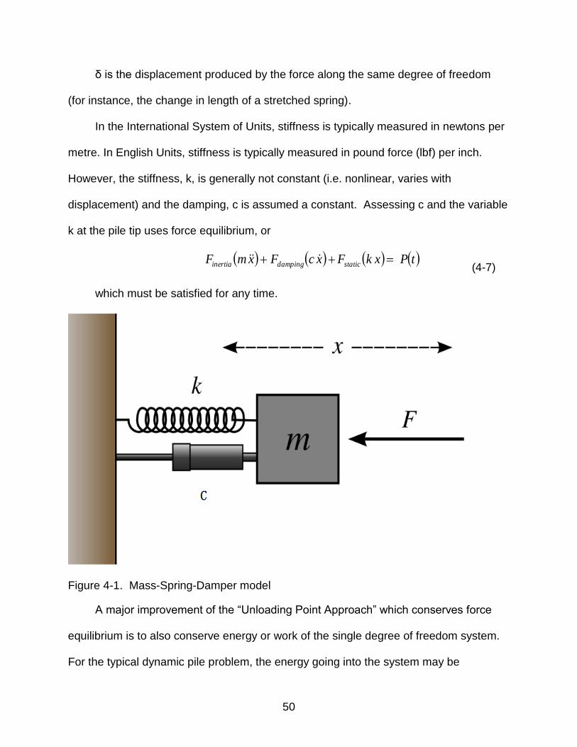
Figure 4-1. Mass-Spring-Damper model

A major improvement of the “Unloading Point Approach” which conserves force

equilibrium is to also conserve energy or work of the single degree of freedom system.

For the typical dynamic pile problem, the energy going into the system may be

51

assessed by the Force measured by tip EDC strain gage and accelerometer. The input

energy must be balanced by the inertia, damping and static energy that occurs as result

of tip acceleration, or

dxtPdxxkxcxm (4-8)

Where x is displacement and is velocity and is acceleration.

To assist with the implementation of the integration as well as improve accuracy

(accelerometer measurements), the integration variable can be changed to time (Liang

& Feeny, 2006) or,

Tt

t

Tt

t

dtxtPdtxxkxcxm

(4-9)

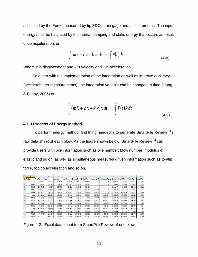
4.1.3 Process of Energy Method

To perform energy method, first thing needed is to generate SmartPile ReviewTM’s

raw data sheet of each blow. As the figure shown below, SmartPile ReviewTM can

provide users with pile information such as pile number, blow number, modulus of

elastic and so on, as well as simultaneous measured driven information such as top/tip

force, top/tip acceleration and so on.

Figure 4-2. Excel data sheet from SmartPile Review of one blow

52

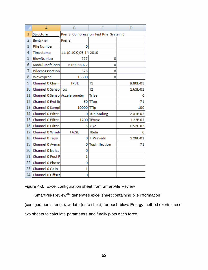
Figure 4-3. Excel configuration sheet from SmartPile Review

SmartPile ReviewTM generates excel sheet containing pile information

(configuration sheet), raw data (data sheet) for each blow. Energy method exerts these

two sheets to calculate parameters and finally plots each force.

53

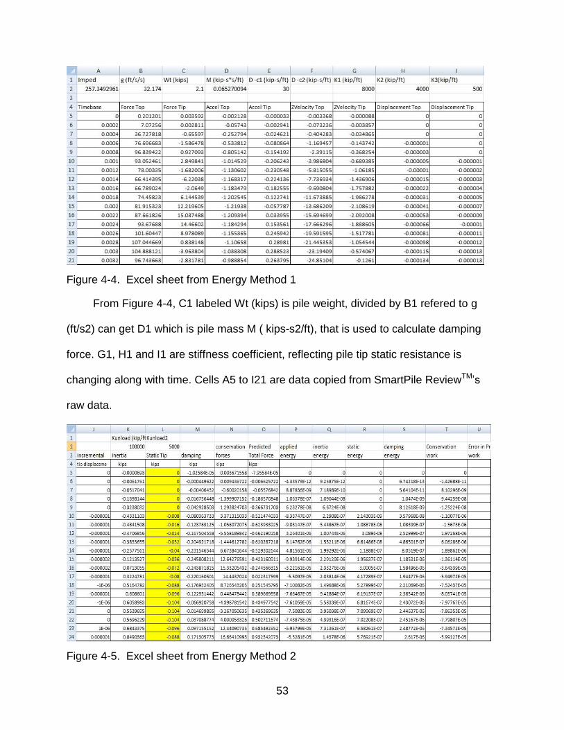
Figure 4-4. Excel sheet from Energy Method 1

From Figure 4-4, C1 labeled Wt (kips) is pile weight, divided by B1 refered to g

(ft/s2) can get D1 which is pile mass M ( kips-s2/ft), that is used to calculate damping

force. G1, H1 and I1 are stiffness coefficient, reflecting pile tip static resistance is

changing along with time. Cells A5 to I21 are data copied from SmartPile ReviewTM’s

raw data.

Figure 4-5. Excel sheet from Energy Method 2

54

From Figure 4-5, it shows all the forces calculated using the raw data from Figure

4-4. As mentioned before, forces acting on the pile tip model are forces input from

hammer (in the energy method sheet, it is directly got from SmartPile ReviewTM called

tip force), damping force (Column M, equals to velocity times damping ratio), static tip

force (Column L, equals to stiffness times tip mass), inertia force (Column K, equals to

acceleration times tip mass). From Column Q to Column T, they are energy measured

from each force. Except for force equilibrium, another equilibrium of pile tip is energy

balance. After calculating all these forces, it’s ready to draw all the forces or energy

together and minimize the error force/energy.

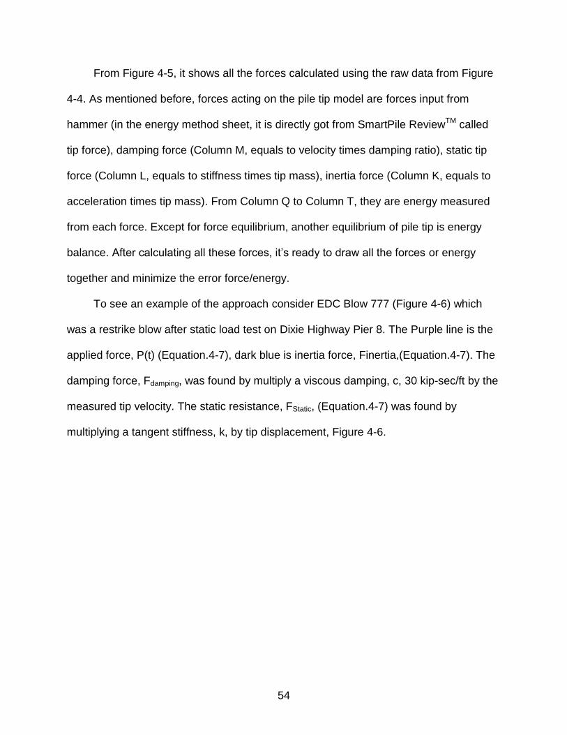
To see an example of the approach consider EDC Blow 777 (Figure 4-6) which

was a restrike blow after static load test on Dixie Highway Pier 8. The Purple line is the

applied force, P(t) (Equation.4-7), dark blue is inertia force, Finertia,(Equation.4-7). The

damping force, Fdamping, was found by multiply a viscous damping, c, 30 kip-sec/ft by the

measured tip velocity. The static resistance, FStatic, (Equation.4-7) was found by

multiplying a tangent stiffness, k, by tip displacement, Figure 4-6.

55

Figure 4-6. EDC Blow 777 Forces vs. Time at Pile Tip of Pier 8

The assessment of c and k begins where the damping and inertia forces are zero

(blue and green lines) in Figures 4-6 (at 0.175 sec 0.023sec and 0.0314sec) and 32 (at

0.0359 ft, 0.0523 ft and 0.0693 ft). For these times and displacements the applied force,

P(t) must equal the static resistance, Fstatic, from equilibrium eq.4-7. Knowing the Fstatic,

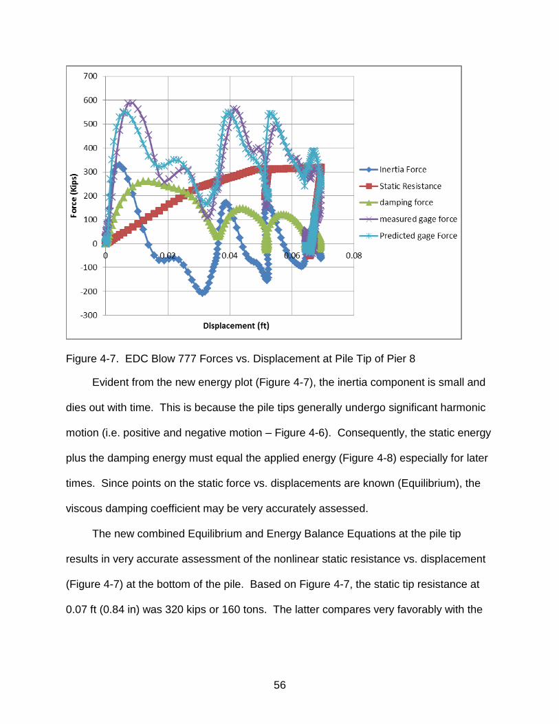
the value of tangent stiffness, k may be assessed (slopes of red line Figure 4-6). Finally,

the value of the viscous damping, c (30 kip-sec/ft) may be determined through the

energy balance at the pile tip from Equation 4-9. Shown in Figure 4-8 is the computed

energy for each component (applied, inertia, damping, and stiffness) as well as the error

(Eapplied – Einertia – Edamping – Estatic).

56

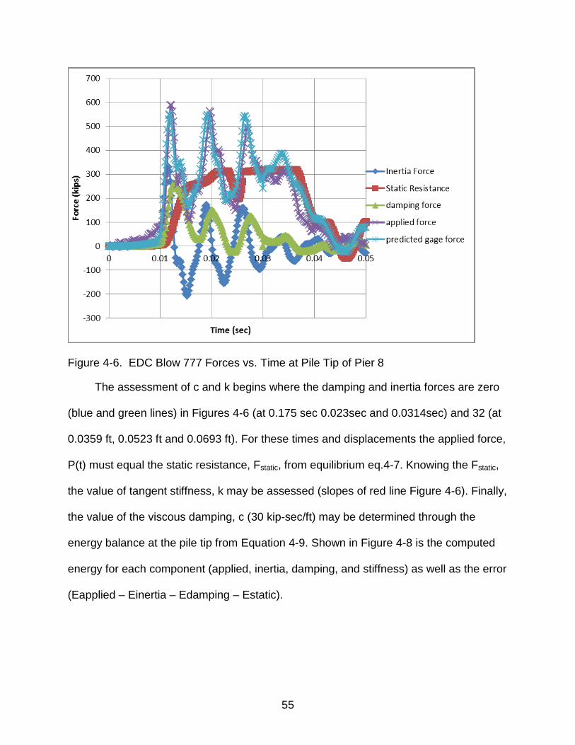
Figure 4-7. EDC Blow 777 Forces vs. Displacement at Pile Tip of Pier 8

Evident from the new energy plot (Figure 4-7), the inertia component is small and

dies out with time. This is because the pile tips generally undergo significant harmonic

motion (i.e. positive and negative motion – Figure 4-6). Consequently, the static energy

plus the damping energy must equal the applied energy (Figure 4-8) especially for later

times. Since points on the static force vs. displacements are known (Equilibrium), the

viscous damping coefficient may be very accurately assessed.

The new combined Equilibrium and Energy Balance Equations at the pile tip

results in very accurate assessment of the nonlinear static resistance vs. displacement

(Figure 4-7) at the bottom of the pile. Based on Figure 4-7, the static tip resistance at

0.07 ft (0.84 in) was 320 kips or 160 tons. The latter compares very favorably with the

57

measured static tip resistance of 336 kip at 0.9 in of movement.

Figure 4-8. EDC Blow 777 Energy vs. Time at Pile Tip of Pier 8

Another example here is blow 779 of Dixie Highway Pier 8, which also shows

energy method performs well.

Figure 4-9. EDC Blow 779 Forces vs. Time at Pile Tip of Pier 8

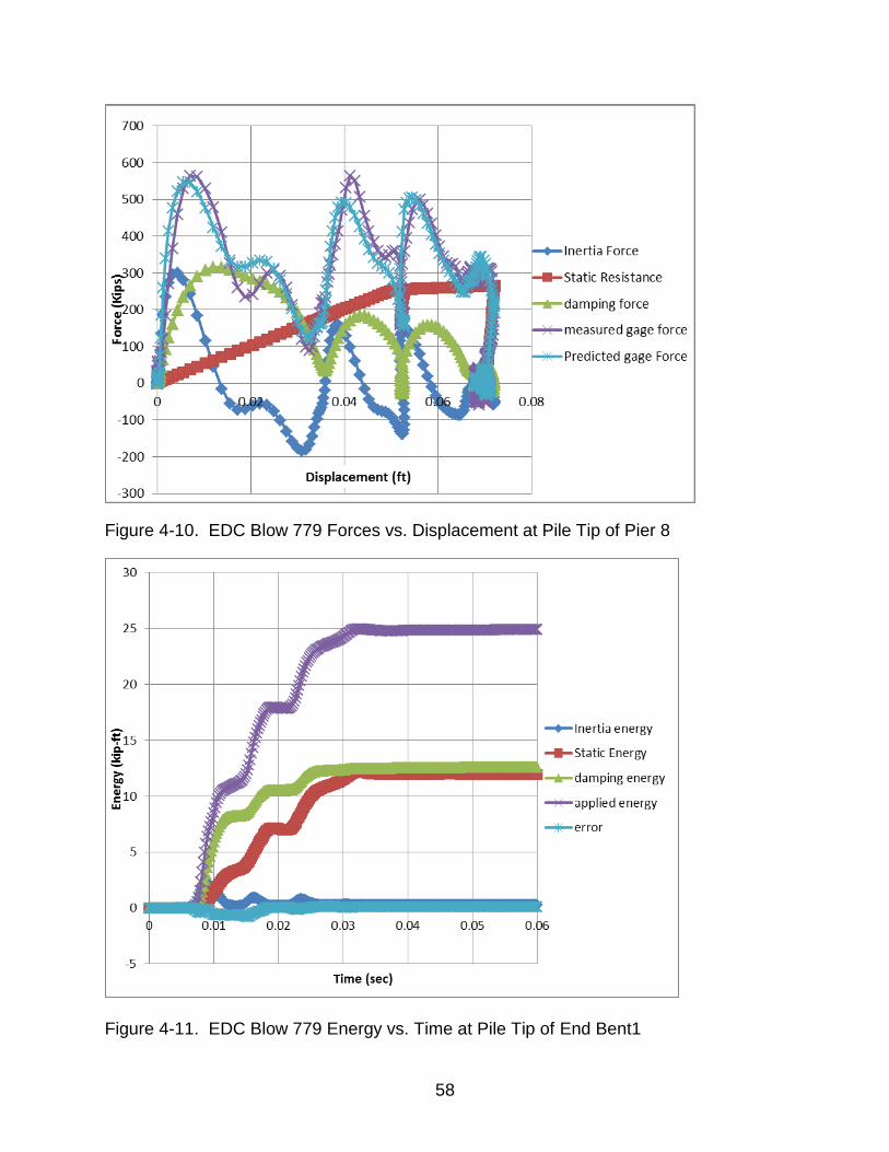
58

Figure 4-10. EDC Blow 779 Forces vs. Displacement at Pile Tip of Pier 8

Figure 4-11. EDC Blow 779 Energy vs. Time at Pile Tip of End Bent1

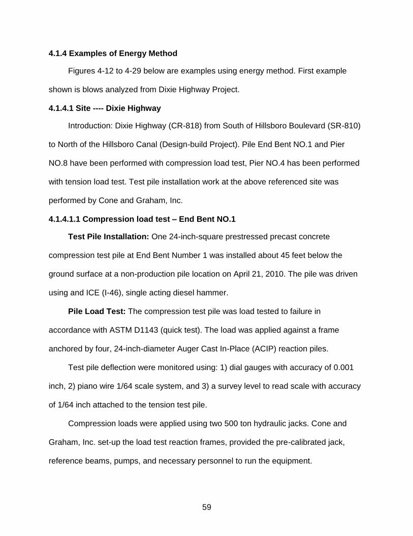
59

4.1.4 Examples of Energy Method

Figures 4-12 to 4-29 below are examples using energy method. First example

shown is blows analyzed from Dixie Highway Project.

4.1.4.1 Site ---- Dixie Highway

Introduction: Dixie Highway (CR-818) from South of Hillsboro Boulevard (SR-810)

to North of the Hillsboro Canal (Design-build Project). Pile End Bent NO.1 and Pier

NO.8 have been performed with compression load test, Pier NO.4 has been performed

with tension load test. Test pile installation work at the above referenced site was

performed by Cone and Graham, Inc.

4.1.4.1.1 Compression load test – End Bent NO.1

Test Pile Installation: One 24-inch-square prestressed precast concrete

compression test pile at End Bent Number 1 was installed about 45 feet below the

ground surface at a non-production pile location on April 21, 2010. The pile was driven

using and ICE (I-46), single acting diesel hammer.

Pile Load Test: The compression test pile was load tested to failure in

accordance with ASTM D1143 (quick test). The load was applied against a frame

anchored by four, 24-inch-diameter Auger Cast In-Place (ACIP) reaction piles.

Test pile deflection were monitored using: 1) dial gauges with accuracy of 0.001

inch, 2) piano wire 1/64 scale system, and 3) a survey level to read scale with accuracy

of 1/64 inch attached to the tension test pile.

Compression loads were applied using two 500 ton hydraulic jacks. Cone and

Graham, Inc. set-up the load test reaction frames, provided the pre-calibrated jack,

reference beams, pumps, and necessary personnel to run the equipment.

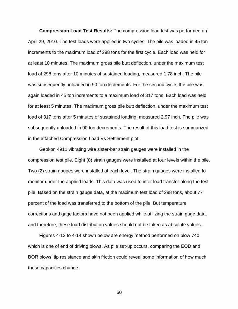
60

Compression Load Test Results: The compression load test was performed on

April 29, 2010. The test loads were applied in two cycles. The pile was loaded in 45 ton

increments to the maximum load of 298 tons for the first cycle. Each load was held for

at least 10 minutes. The maximum gross pile butt deflection, under the maximum test

load of 298 tons after 10 minutes of sustained loading, measured 1.78 inch. The pile

was subsequently unloaded in 90 ton decrements. For the second cycle, the pile was

again loaded in 45 ton increments to a maximum load of 317 tons. Each load was held

for at least 5 minutes. The maximum gross pile butt deflection, under the maximum test

load of 317 tons after 5 minutes of sustained loading, measured 2.97 inch. The pile was

subsequently unloaded in 90 ton decrements. The result of this load test is summarized

in the attached Compression Load Vs Settlement plot.

Geokon 4911 vibrating wire sister-bar strain gauges were installed in the

compression test pile. Eight (8) strain gauges were installed at four levels within the pile.

Two (2) strain gauges were installed at each level. The strain gauges were installed to

monitor under the applied loads. This data was used to infer load transfer along the test

pile. Based on the strain gauge data, at the maximum test load of 298 tons, about 77

percent of the load was transferred to the bottom of the pile. But temperature

corrections and gage factors have not been applied while utilizing the strain gage data,

and therefore, these load distribution values should not be taken as absolute values.

Figures 4-12 to 4-14 shown below are energy method performed on blow 740

which is one of end of driving blows. As pile set-up occurs, comparing the EOD and

BOR blows’ tip resistance and skin friction could reveal some information of how much

these capacities change.

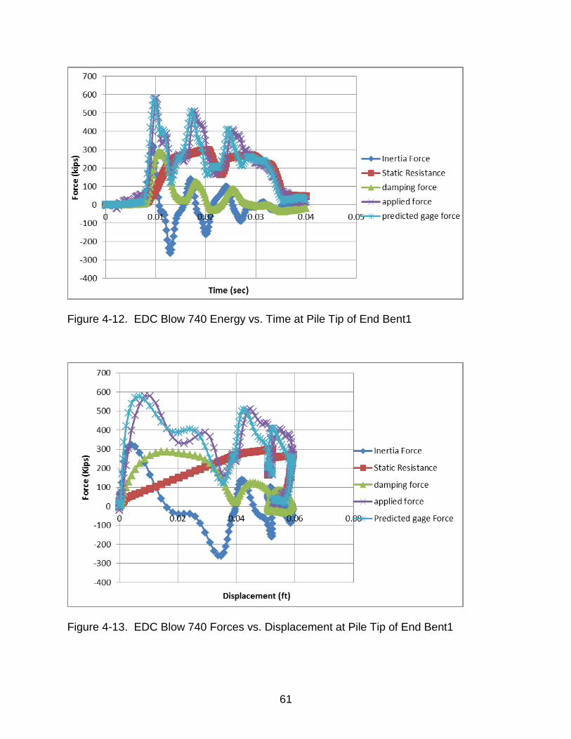
61

Figure 4-12. EDC Blow 740 Energy vs. Time at Pile Tip of End Bent1

Figure 4-13. EDC Blow 740 Forces vs. Displacement at Pile Tip of End Bent1

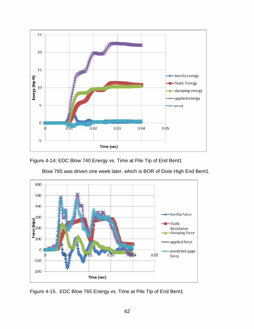
62

Figure 4-14: EDC Blow 740 Energy vs. Time at Pile Tip of End Bent1

Blow 765 was driven one week later, which is BOR of Dixie High End Bent1.

Figure 4-15. EDC Blow 765 Energy vs. Time at Pile Tip of End Bent1

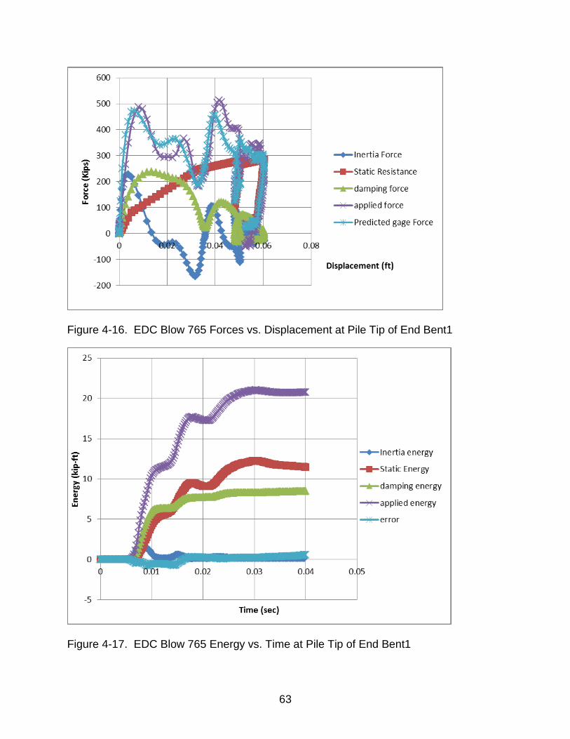
63

Figure 4-16. EDC Blow 765 Forces vs. Displacement at Pile Tip of End Bent1

Figure 4-17. EDC Blow 765 Energy vs. Time at Pile Tip of End Bent1

64

For Dixie highway End Bent1, 10 re-strike blows just before and after the load test

for comparison with one another as well as with the measured static tip resistance from

the load test. The specific results of one of the re-strike blow are presented here in

detail for discussion. Energy method performed for other 9 blows will be presented in

Apendix A.

4.1.4.1.2 Compression load test – Pier NO.8

Test pile installation: One 24-inch-square prestressed precast concrete

compression test pile at Pier Number 8 was installed about 49 feet below the ground

surface at a non-production pile location on May 6, 2010. The pile was driven using an

ICE (I-46), single acting diesel hammer.

Pile Load Test: The compression test pile was load tested to failure in accordace

with ASTM D1143 (quick test). The load was applied against a frame anchored by four,

24-inch-diameter Auger Cast In-Place (ACIP) reaction piles.

Test pile deflections were monitored using: 1) dial gauges with accuracy of 0.001

inch, 2) piano wire 1/64 scale system, and 3) a survey level to read scale with accuracy

of 1/64 inch attached to the hydraulic jack.

Compression loads were applied using two 500 ton hydraulic jackes. Cone and

Graham, Inc. set-up the load test reaction frames, provided the pre-calibrated jack,

reference beams, pumps, and necessary personnel to run the equipment.

Compression Load Test Results: The compression load test was performed on

May 12, 2010. The test loads were applied in two cycles. The pile was loaded in 45 ton

increments to the maximum load of 255 tons for the first cycle. Each load was held for

at least 10 minutes. The maximum gross pile butt deflection, under the maximum test

load of 255 tons after 10 minutes of sustained loading, measured 1.69 inch. The pile

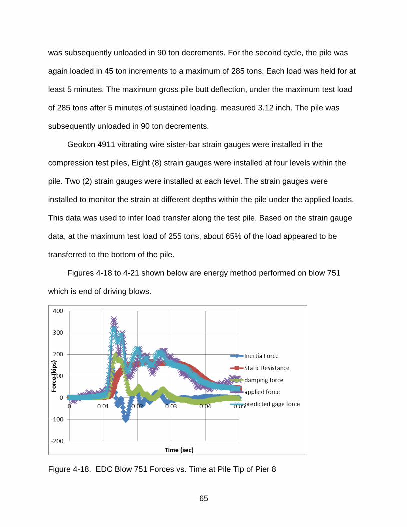
65

was subsequently unloaded in 90 ton decrements. For the second cycle, the pile was

again loaded in 45 ton increments to a maximum of 285 tons. Each load was held for at

least 5 minutes. The maximum gross pile butt deflection, under the maximum test load

of 285 tons after 5 minutes of sustained loading, measured 3.12 inch. The pile was

subsequently unloaded in 90 ton decrements.

Geokon 4911 vibrating wire sister-bar strain gauges were installed in the

compression test piles, Eight (8) strain gauges were installed at four levels within the

pile. Two (2) strain gauges were installed at each level. The strain gauges were

installed to monitor the strain at different depths within the pile under the applied loads.

This data was used to infer load transfer along the test pile. Based on the strain gauge

data, at the maximum test load of 255 tons, about 65% of the load appeared to be

transferred to the bottom of the pile.

Figures 4-18 to 4-21 shown below are energy method performed on blow 751

which is end of driving blows.

Figure 4-18. EDC Blow 751 Forces vs. Time at Pile Tip of Pier 8

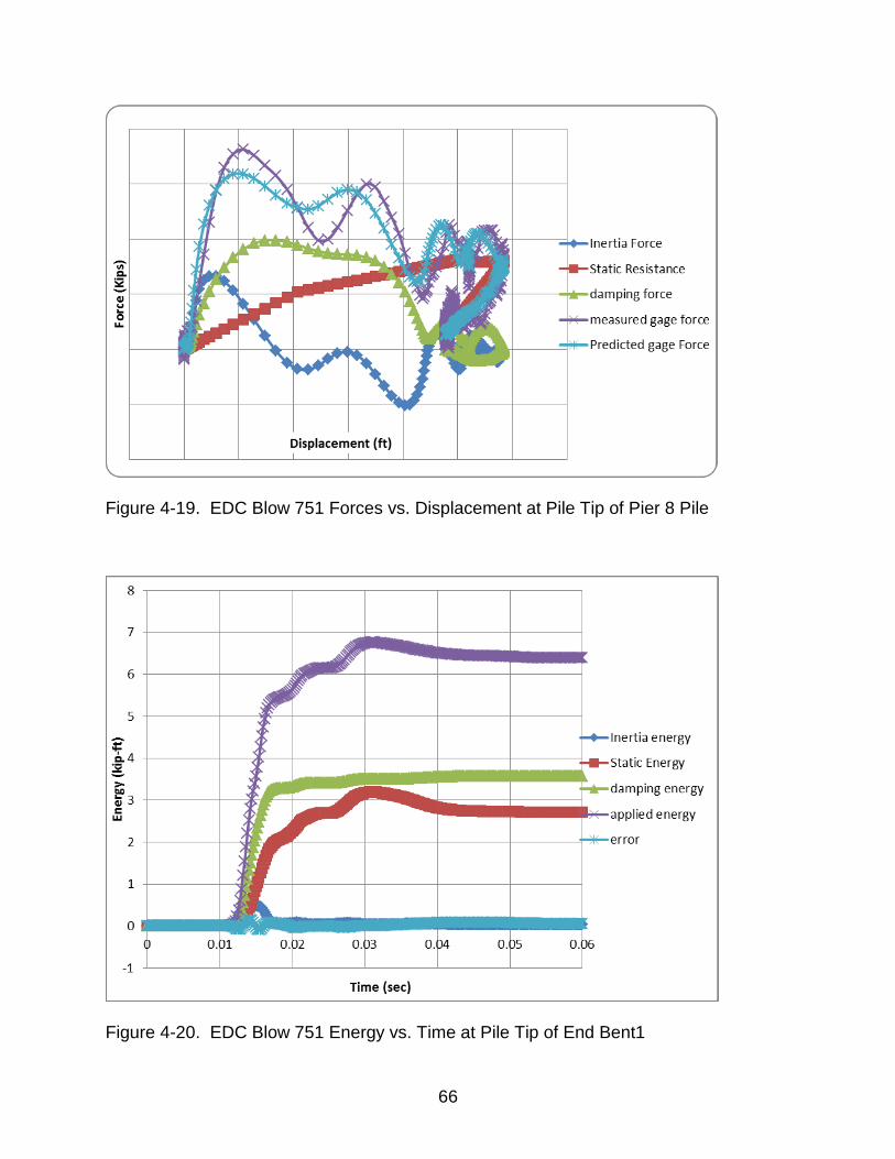
66

Figure 4-19. EDC Blow 751 Forces vs. Displacement at Pile Tip of Pier 8 Pile

Figure 4-20. EDC Blow 751 Energy vs. Time at Pile Tip of End Bent1

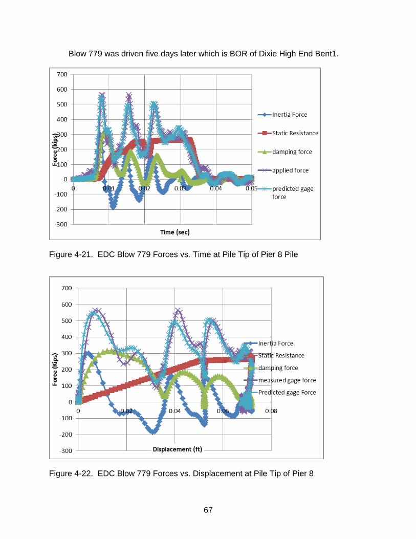
67

Blow 779 was driven five days later which is BOR of Dixie High End Bent1.

Figure 4-21. EDC Blow 779 Forces vs. Time at Pile Tip of Pier 8 Pile

Figure 4-22. EDC Blow 779 Forces vs. Displacement at Pile Tip of Pier 8

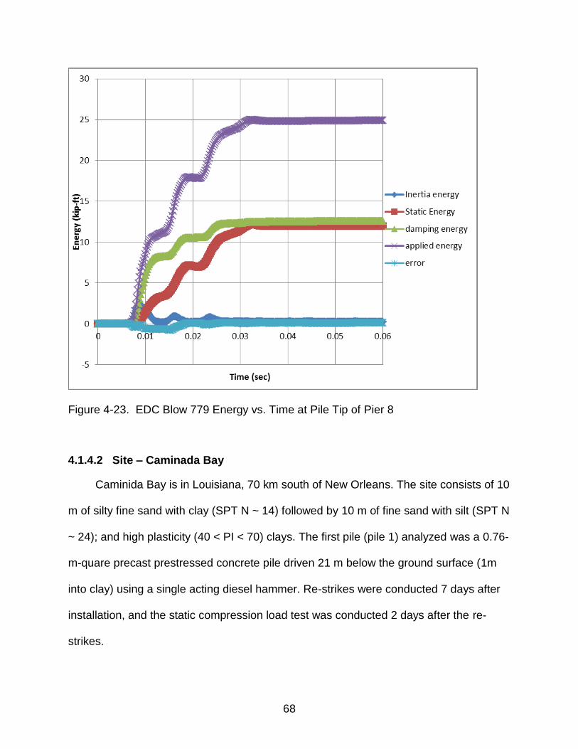
68

Figure 4-23. EDC Blow 779 Energy vs. Time at Pile Tip of Pier 8

4.1.4.2 Site – Caminada Bay

Caminida Bay is in Louisiana, 70 km south of New Orleans. The site consists of 10

m of silty fine sand with clay (SPT N ~ 14) followed by 10 m of fine sand with silt (SPT N

~ 24); and high plasticity (40 < PI < 70) clays. The first pile (pile 1) analyzed was a 0.76-

m-quare precast prestressed concrete pile driven 21 m below the ground surface (1m

into clay) using a single acting diesel hammer. Re-strikes were conducted 7 days after

installation, and the static compression load test was conducted 2 days after the re-

strikes.

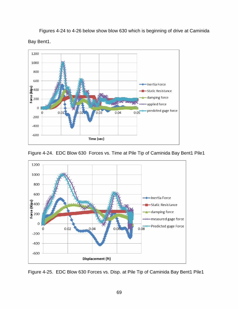
69

Figures 4-24 to 4-26 below show blow 630 which is beginning of drive at Caminida

Bay Bent1.

Figure 4-24. EDC Blow 630 Forces vs. Time at Pile Tip of Caminida Bay Bent1 Pile1

Figure 4-25. EDC Blow 630 Forces vs. Disp. at Pile Tip of Caminida Bay Bent1 Pile1

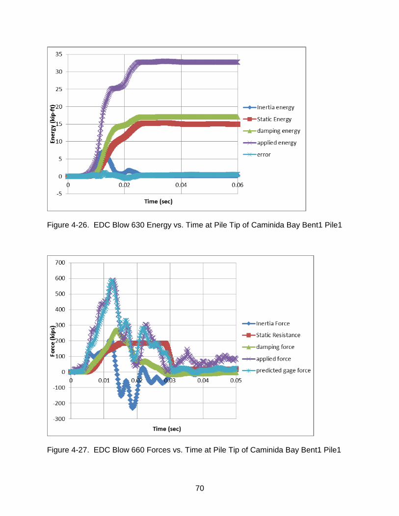
70

Figure 4-26. EDC Blow 630 Energy vs. Time at Pile Tip of Caminida Bay Bent1 Pile1

Figure 4-27. EDC Blow 660 Forces vs. Time at Pile Tip of Caminida Bay Bent1 Pile1

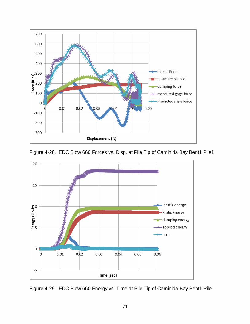
71

Figure 4-28. EDC Blow 660 Forces vs. Disp. at Pile Tip of Caminida Bay Bent1 Pile1

Figure 4-29. EDC Blow 660 Energy vs. Time at Pile Tip of Caminida Bay Bent1 Pile1

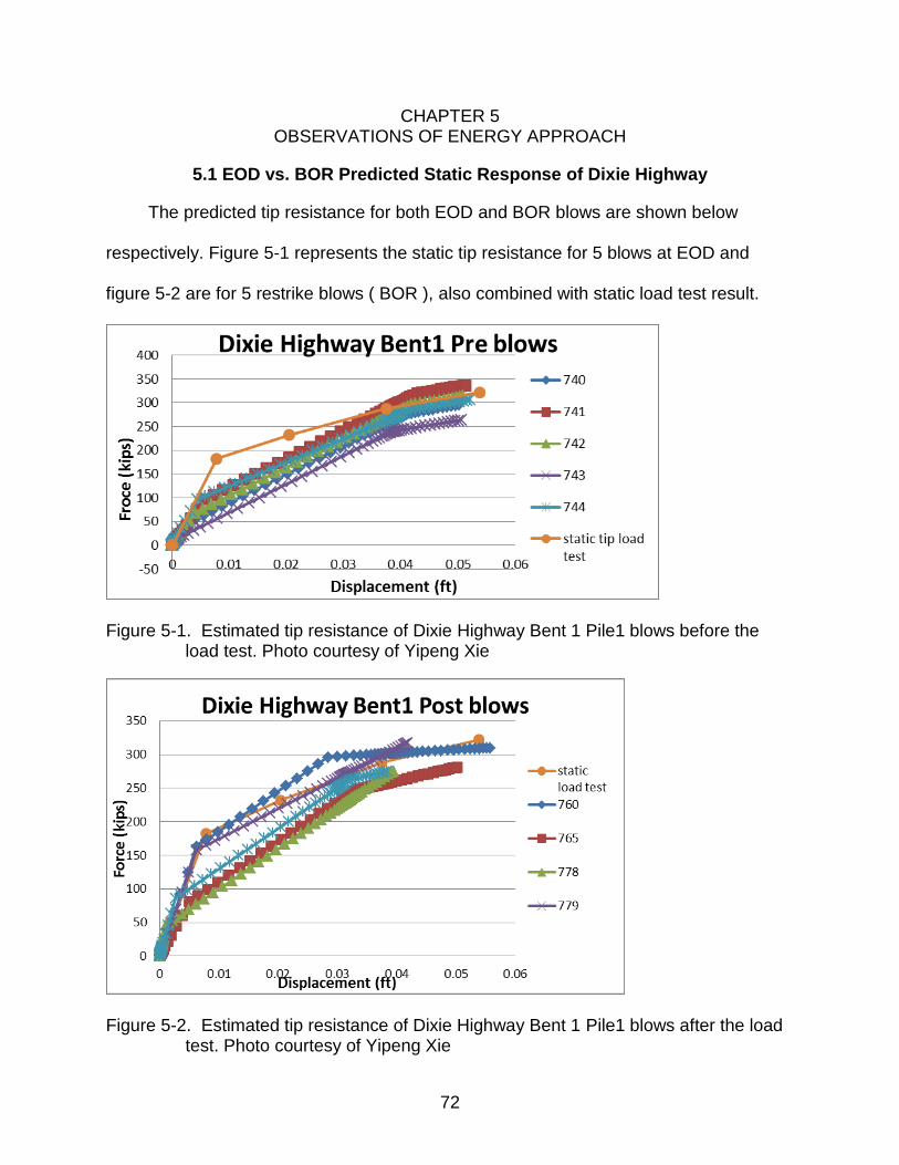
72

CHAPTER 5 OBSERVATIONS OF ENERGY APPROACH

5.1 EOD vs. BOR Predicted Static Response of Dixie Highway

The predicted tip resistance for both EOD and BOR blows are shown below

respectively. Figure 5-1 represents the static tip resistance for 5 blows at EOD and

figure 5-2 are for 5 restrike blows ( BOR ), also combined with static load test result.

Figure 5-1. Estimated tip resistance of Dixie Highway Bent 1 Pile1 blows before the

load test. Photo courtesy of Yipeng Xie

Figure 5-2. Estimated tip resistance of Dixie Highway Bent 1 Pile1 blows after the load

test. Photo courtesy of Yipeng Xie

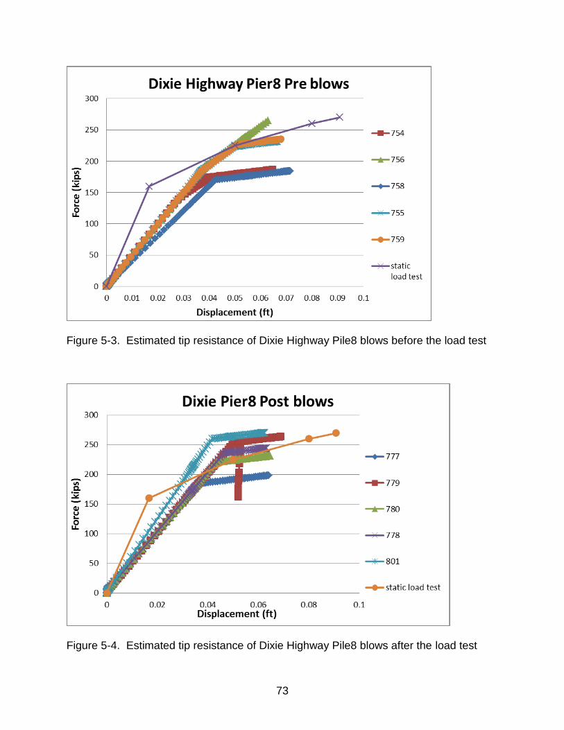
73

Figure 5-3. Estimated tip resistance of Dixie Highway Pile8 blows before the load test

Figure 5-4. Estimated tip resistance of Dixie Highway Pile8 blows after the load test

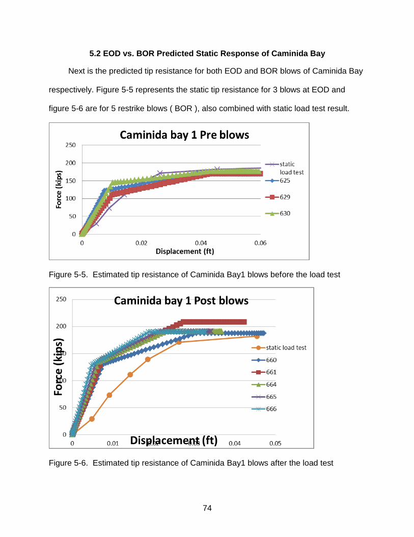
74

5.2 EOD vs. BOR Predicted Static Response of Caminida Bay

Next is the predicted tip resistance for both EOD and BOR blows of Caminida Bay

respectively. Figure 5-5 represents the static tip resistance for 3 blows at EOD and

figure 5-6 are for 5 restrike blows ( BOR ), also combined with static load test result.

Figure 5-5. Estimated tip resistance of Caminida Bay1 blows before the load test

Figure 5-6. Estimated tip resistance of Caminida Bay1 blows after the load test

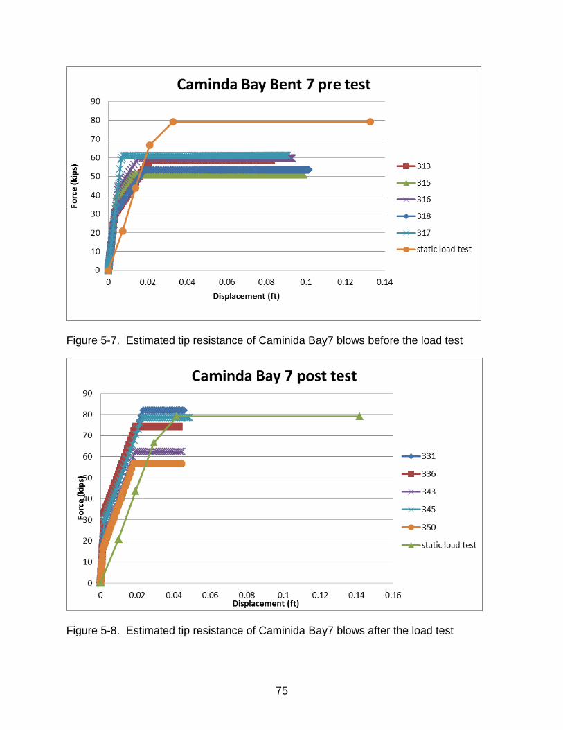
75

Figure 5-7. Estimated tip resistance of Caminida Bay7 blows before the load test

Figure 5-8. Estimated tip resistance of Caminida Bay7 blows after the load test

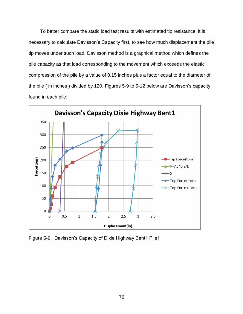
76

To better compare the static load test results with estimated tip resistance, it is

necessary to calculate Davisson’s Capacity first, to see how much displacement the pile

tip moves under such load. Davisson method is a graphical method which defines the

pile capacity as that load corresponding to the movement which exceeds the elastic

compression of the pile by a value of 0.15 inches plus a factor equal to the diameter of

the pile ( in inches ) divided by 120. Figures 5-9 to 5-12 below are Davisson’s capacity

found in each pile:

Figure 5-9. Davisson’s Capacity of Dixie Highway Bent1 Pile1

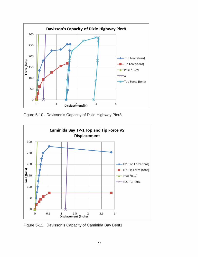
77

Figure 5-10. Davisson’s Capacity of Dixie Highway Pier8

Figure 5-11. Davisson’s Capacity of Caminida Bay Bent1

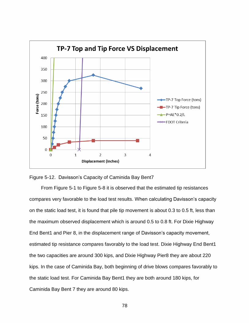
78

Figure 5-12. Davisson’s Capacity of Caminida Bay Bent7

From Figure 5-1 to Figure 5-8 it is observed that the estimated tip resistances

compares very favorable to the load test results. When calculating Davisson’s capacity

on the static load test, it is found that pile tip movement is about 0.3 to 0.5 ft, less than

the maximum observed displacement which is around 0.5 to 0.8 ft. For Dixie Highway

End Bent1 and Pier 8, in the displacement range of Davisson’s capacity movement,

estimated tip resistance compares favorably to the load test. Dixie Highway End Bent1

the two capacities are around 300 kips, and Dixie Highway Pier8 they are about 220

kips. In the case of Caminida Bay, both beginning of drive blows compares favorably to

the static load test. For Caminida Bay Bent1 they are both around 180 kips, for

Caminida Bay Bent 7 they are around 80 kips.

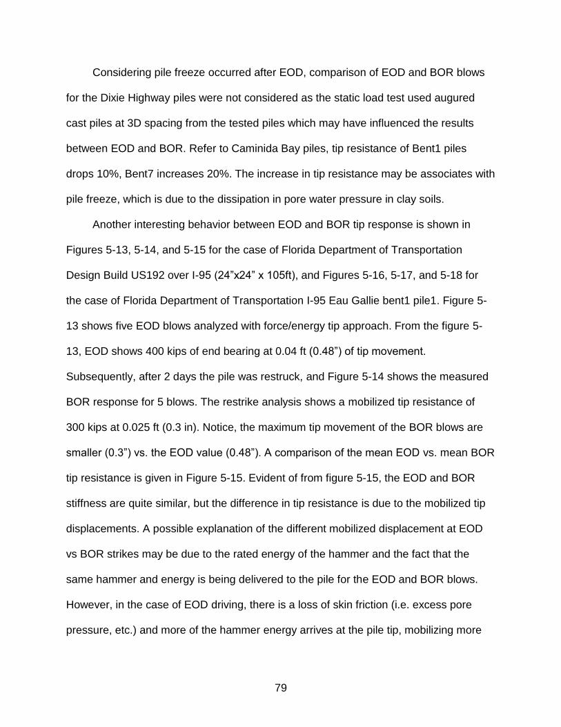
79

Considering pile freeze occurred after EOD, comparison of EOD and BOR blows

for the Dixie Highway piles were not considered as the static load test used augured

cast piles at 3D spacing from the tested piles which may have influenced the results

between EOD and BOR. Refer to Caminida Bay piles, tip resistance of Bent1 piles

drops 10%, Bent7 increases 20%. The increase in tip resistance may be associates with

pile freeze, which is due to the dissipation in pore water pressure in clay soils.

Another interesting behavior between EOD and BOR tip response is shown in

Figures 5-13, 5-14, and 5-15 for the case of Florida Department of Transportation

Design Build US192 over I-95 (24”x24” x 105ft), and Figures 5-16, 5-17, and 5-18 for

the case of Florida Department of Transportation I-95 Eau Gallie bent1 pile1. Figure 5-

13 shows five EOD blows analyzed with force/energy tip approach. From the figure 5-

13, EOD shows 400 kips of end bearing at 0.04 ft (0.48”) of tip movement.

Subsequently, after 2 days the pile was restruck, and Figure 5-14 shows the measured

BOR response for 5 blows. The restrike analysis shows a mobilized tip resistance of

300 kips at 0.025 ft (0.3 in). Notice, the maximum tip movement of the BOR blows are

smaller (0.3”) vs. the EOD value (0.48”). A comparison of the mean EOD vs. mean BOR

tip resistance is given in Figure 5-15. Evident of from figure 5-15, the EOD and BOR

stiffness are quite similar, but the difference in tip resistance is due to the mobilized tip

displacements. A possible explanation of the different mobilized displacement at EOD

vs BOR strikes may be due to the rated energy of the hammer and the fact that the

same hammer and energy is being delivered to the pile for the EOD and BOR blows.

However, in the case of EOD driving, there is a loss of skin friction (i.e. excess pore

pressure, etc.) and more of the hammer energy arrives at the pile tip, mobilizing more

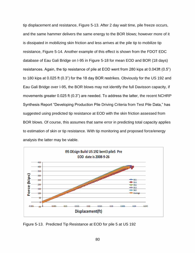
80

tip displacement and resistance, Figure 5-13. After 2 day wait time, pile freeze occurs,

and the same hammer delivers the same energy to the BOR blows; however more of it

is dissipated in mobilizing skin friction and less arrives at the pile tip to mobilize tip

resistance, Figure 5-14. Another example of this effect is shown from the FDOT EDC

database of Eau Gali Bridge on I-95 in Figure 5-18 for mean EOD and BOR (18 days)

resistances. Again, the tip resistance of pile at EOD went from 280 kips at 0.043ft (0.5”)

to 180 kips at 0.025 ft (0.3”) for the 18 day BOR restrikes. Obviously for the US 192 and

Eau Gali Bridge over I-95, the BOR blows may not identify the full Davisson capacity, if

movements greater 0.025 ft (0.3”) are needed. To address the latter, the recent NCHRP

Synthesis Report “Developing Production Pile Driving Criteria from Test Pile Data,” has

suggested using predicted tip resistance at EOD with the skin friction assessed from

BOR blows. Of course, this assumes that same error in predicting total capacity applies

to estimation of skin or tip resistance. With tip monitoring and proposed force/energy

analysis the latter may be viable.

Figure 5-13. Predicted Tip Resistance at EOD for pile 5 at US 192

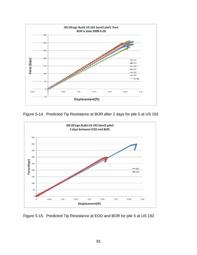
81

Figure 5-14. Predicted Tip Resistance at BOR after 2 days for pile 5 at US 192

Figure 5-15. Predicted Tip Resistance at EOD and BOR for pile 5 at US 192

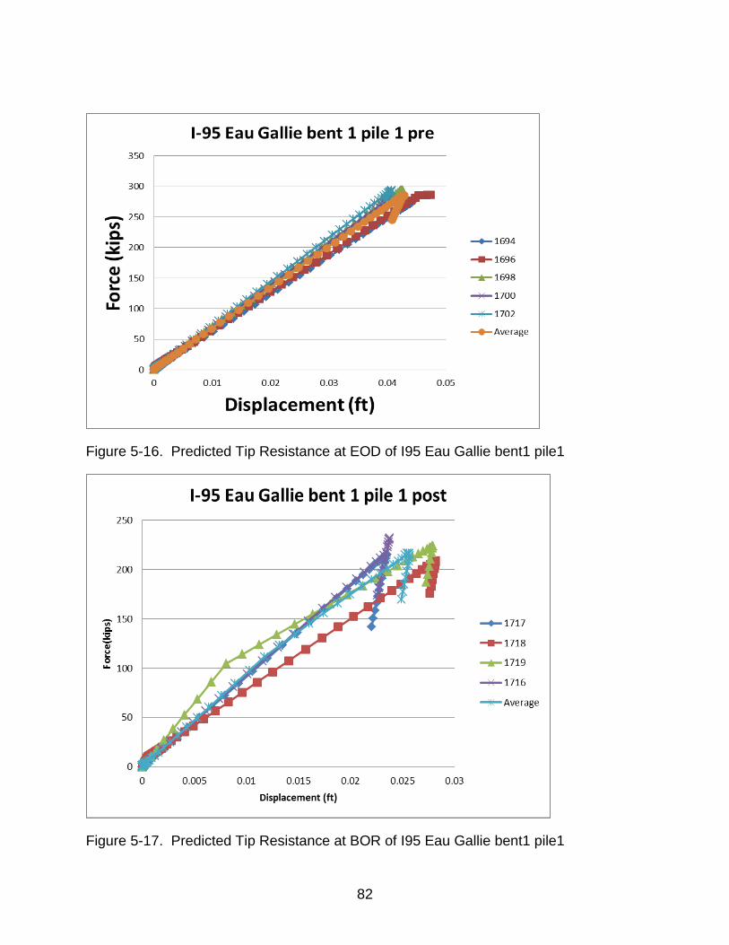
82

Figure 5-16. Predicted Tip Resistance at EOD of I95 Eau Gallie bent1 pile1

Figure 5-17. Predicted Tip Resistance at BOR of I95 Eau Gallie bent1 pile1

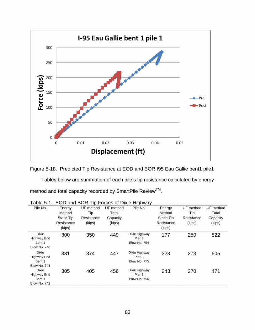
83

Figure 5-18. Predicted Tip Resistance at EOD and BOR I95 Eau Gallie bent1 pile1

Tables below are summation of each pile’s tip resistance calculated by energy

method and total capacity recorded by SmartPile ReviewTM.

Table 5-1. EOD and BOR Tip Forces of Dixie Highway Pile No. Energy

Method

Static Tip

Resistance

(kips)

UF method

Tip

Resistance

(kips)

UF method

Total

Capacity

(kips)

Pile No. Energy

Method

Static Tip

Resistance

(kips)

UF method

Tip

Resistance

(kips)

UF method

Total

Capacity

(kips)

Dixie

Highway End

Bent 1

Blow No. 740

300 350 449 Dixie Highway

Pier 8

Blow No. 754

177 250 522

Dixie

Highway End

Bent 1

Blow No. 741

331 374 447 Dixie Highway

Pier 8

Blow No. 755

228 273 505

Dixie

Highway End

Bent 1

Blow No. 742

305 405 456 Dixie Highway

Pier 8

Blow No. 756

243 270 471

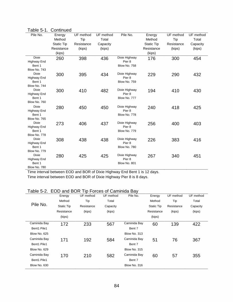
84

Table 5-1. Continued Pile No. Energy

Method

Static Tip

Resistance

(kips)

UF method

Tip

Resistance

(kips)

UF method

Total

Capacity

(kips)

Pile No. Energy

Method

Static Tip

Resistance

(kips)

UF method

Tip

Resistance

(kips)

UF method

Total

Capacity

(kips)

Dixie

Highway End

Bent 1

Blow No. 743

260 398 436 Dixie Highway

Pier 8

Blow No. 758

176 300 454

Dixie

Highway End

Bent 1

Blow No. 744

300 395 434 Dixie Highway

Pier 8

Blow No. 759

229 290 432

Dixie

Highway End

Bent 1

Blow No. 760

300 410 482 Dixie Highway

Pier 8

Blow No. 777

194 410 430

Dixie

Highway End

Bent 1

Blow No. 765

280 450 450 Dixie Highway

Pier 8

Blow No. 778

240 418 425

Dixie

Highway End

Bent 1

Blow No. 778

273 406 437 Dixie Highway

Pier 8

Blow No. 779

256 400 403

Dixie

Highway End

Bent 1

Blow No. 779

308 438 438 Dixie Highway

Pier 8

Blow No. 780

226 383 416

Dixie

Highway End

Bent 1

Blow No. 780

280 425 425 Dixie Highway

Pier 8

Blow No. 801

267 340 451

Time interval between EOD and BOR of Dixie Highway End Bent 1 is 12 days.

Time interval between EOD and BOR of Dixie Highway Pier 8 is 8 days.

Table 5-2. EOD and BOR Tip Forces of Caminida Bay

Pile No.

Energy

Method

Static Tip

Resistance

(kips)

UF method

Tip

Resistance

(kips)

UF method

Total

Capacity

(kips)

Pile No. Energy

Method

Static Tip

Resistance

(kips)

UF method

Tip

Resistance

(kips)

UF method

Total

Capacity

(kips)

Caminida Bay

Bent1 Pile1

Blow No. 625

172 233 567 Caminida Bay

Bent 7

Blow No. 313

60 139 422

Caminida Bay

Bent1 Pile1

Blow No. 629

171 192 584 Caminida Bay

Bent 7

Blow No. 315

51 76 367

Caminida Bay

Bent1 Pile1

Blow No. 630

170 210 582 Caminida Bay

Bent 7

Blow No. 316

60 57 355

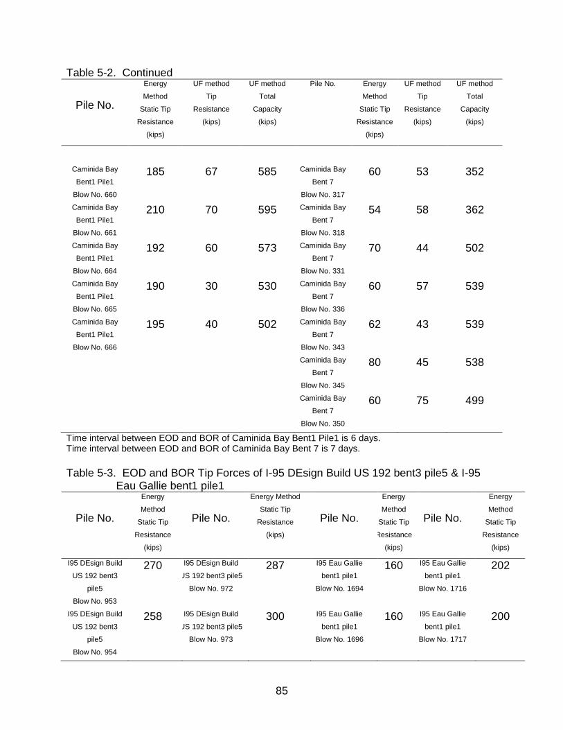
85

Table 5-2. Continued

Pile No.

Energy

Method

Static Tip

Resistance

(kips)

UF method

Tip

Resistance

(kips)

UF method

Total

Capacity

(kips)

Pile No. Energy

Method

Static Tip

Resistance

(kips)

UF method

Tip

Resistance

(kips)

UF method

Total

Capacity

(kips)

Caminida Bay

Bent1 Pile1

Blow No. 660

185 67 585 Caminida Bay

Bent 7

Blow No. 317

60 53 352

Caminida Bay

Bent1 Pile1

Blow No. 661

210

70 595 Caminida Bay

Bent 7

Blow No. 318

54 58 362

Caminida Bay

Bent1 Pile1

Blow No. 664

192 60 573 Caminida Bay

Bent 7

Blow No. 331

70 44 502

Caminida Bay

Bent1 Pile1

Blow No. 665

190 30 530 Caminida Bay

Bent 7

Blow No. 336

60 57 539

Caminida Bay

Bent1 Pile1

Blow No. 666

195 40 502 Caminida Bay

Bent 7

Blow No. 343

62 43 539

Caminida Bay

Bent 7

Blow No. 345

80 45 538

Caminida Bay

Bent 7

Blow No. 350

60 75 499

Time interval between EOD and BOR of Caminida Bay Bent1 Pile1 is 6 days. Time interval between EOD and BOR of Caminida Bay Bent 7 is 7 days.

Table 5-3. EOD and BOR Tip Forces of I-95 DEsign Build US 192 bent3 pile5 & I-95

Eau Gallie bent1 pile1

Pile No.

Energy

Method

Static Tip

Resistance

(kips)

Pile No.

Energy Method

Static Tip

Resistance

(kips)

Pile No.

Energy

Method

Static Tip

Resistance

(kips)

Pile No.

Energy

Method

Static Tip

Resistance

(kips)

I95 DEsign Build

US 192 bent3

pile5

Blow No. 953

270 I95 DEsign Build

US 192 bent3 pile5

Blow No. 972

287 I95 Eau Gallie

bent1 pile1

Blow No. 1694

160 I95 Eau Gallie

bent1 pile1

Blow No. 1716

202

I95 DEsign Build

US 192 bent3

pile5

Blow No. 954

258 I95 DEsign Build

US 192 bent3 pile5

Blow No. 973

300 I95 Eau Gallie

bent1 pile1

Blow No. 1696

160 I95 Eau Gallie

bent1 pile1

Blow No. 1717

200

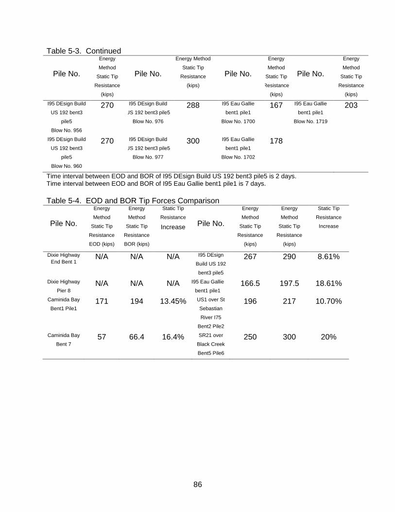
86

Table 5-3. Continued

Pile No.

Energy

Method

Static Tip

Resistance

(kips)

Pile No.

Energy Method

Static Tip

Resistance

(kips)

Pile No.

Energy

Method

Static Tip

Resistance

(kips)

Pile No.

Energy

Method

Static Tip

Resistance

(kips)

I95 DEsign Build

US 192 bent3

pile5

Blow No. 956

270 I95 DEsign Build

US 192 bent3 pile5

Blow No. 976

288 I95 Eau Gallie

bent1 pile1

Blow No. 1700

167 I95 Eau Gallie

bent1 pile1

Blow No. 1719

203

I95 DEsign Build

US 192 bent3

pile5

Blow No. 960

270 I95 DEsign Build

US 192 bent3 pile5

Blow No. 977

300 I95 Eau Gallie

bent1 pile1

Blow No. 1702

178

Time interval between EOD and BOR of I95 DEsign Build US 192 bent3 pile5 is 2 days. Time interval between EOD and BOR of I95 Eau Gallie bent1 pile1 is 7 days.

Table 5-4. EOD and BOR Tip Forces Comparison

Pile No.

Energy

Method

Static Tip

Resistance

EOD (kips)

Energy

Method

Static Tip

Resistance

BOR (kips)

Static Tip

Resistance

Increase

Pile No.

Energy

Method

Static Tip

Resistance

(kips)

Energy

Method

Static Tip

Resistance

(kips)

Static Tip

Resistance

Increase

Dixie Highway

End Bent 1 N/A N/A N/A I95 DEsign

Build US 192

bent3 pile5

267 290 8.61%

Dixie Highway

Pier 8

N/A N/A N/A I95 Eau Gallie

bent1 pile1 166.5 197.5 18.61%

Caminida Bay

Bent1 Pile1

171 194 13.45% US1 over St

Sebastian

River I75

Bent2 Pile2

196 217 10.70%

Caminida Bay

Bent 7

57 66.4 16.4% SR21 over

Black Creek

Bent5 Pile6

250 300 20%

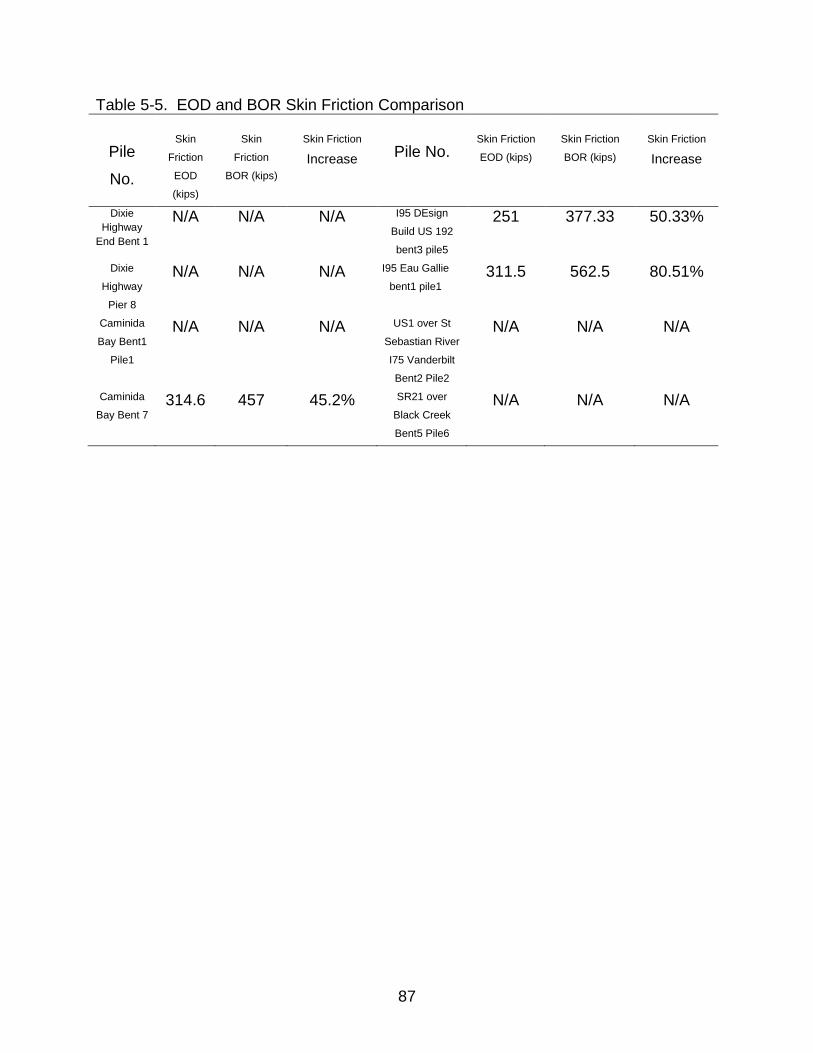
87

Table 5-5. EOD and BOR Skin Friction Comparison

Pile

No.

Skin

Friction

EOD

(kips)

Skin

Friction

BOR (kips)

Skin Friction

Increase

Pile No.

Skin Friction

EOD (kips)

Skin Friction

BOR (kips)

Skin Friction

Increase

Dixie

Highway

End Bent 1

N/A N/A N/A I95 DEsign

Build US 192

bent3 pile5

251 377.33 50.33%

Dixie

Highway

Pier 8

N/A N/A N/A I95 Eau Gallie

bent1 pile1 311.5 562.5 80.51%

Caminida

Bay Bent1

Pile1

N/A N/A N/A US1 over St

Sebastian River

I75 Vanderbilt

Bent2 Pile2

N/A N/A N/A

Caminida

Bay Bent 7

314.6 457 45.2% SR21 over

Black Creek

Bent5 Pile6

N/A N/A N/A

88

CHAPTER 6 CONCLUSION

6.1 Summary

In this study, a completely new method of assessing pile tip static resistance called

energy method has been raised, and by given different test sites for investigation,

energy method is proved to be feasible and efficient. Advantages of this method are

obvious:

It could be done by researchers manually. It based on excel sheet and easy to

learn. The more experience researcher gains, the shorter operating time it takes. Or, it

also could be done automatically by computer once the coding is finished.

Energy method’s results are shown both in the format of numbers and figures,

researchers can read the forces directly from plots without confusion.

Comparing to static load test, dynamic test is convenient and less cost. To get

static tip resistance from dynamic test is always reseachers’ preference. Energy method

uses the data collected from dynamic testing, providing with a guaranteed static tip

force.

As the theories of energy method is force equilibrium and energy equilibrium, and

those equilibrium should be satisfied any time of driving, this method could be applied at

each blow, which means it can calculated static tip resistance either from EOD or BOR.

As pile set-up observed and validated from more and more researchers

nowadays, energy method’s finding can lead to a deeper understanding of it. From the

piles analysed using energy method, static tip resistance seem not to change very much

compared to the skin friction, which most geotechnical researchers agree that is the

main reason contributing to the increase of the pile total capacities. Although pile set-

89

up’s mechanism is still under investigating, results from energy method can provide

some clues of assessing the set-up factor. What we choose here is blows from EOD

and BOR period, usually the time interval between these two phases are several days

long. So it guarantees most of the pile set-up will develop during this time interval. At

the same time, the time when hammer stops hitting is less than one hour is also

considered, and pile set-up is still observed for most cases. Data performed with energy

method compared to static load test results are quite agreeable, which means this

method could be used in future studies.

6.2 Recommendations

For this thesis energy method’s raw data sources are all from SmartPile

ReviewTM’s excel sheets. PDA nowadays is common dynamic testing equipment around

America, so performing energy method with PDA’s outputs will be put into

consideration. Also, to accelerate the calculation, computer automatically run will surely

reduce the time cost, and also provide with more standardized results.

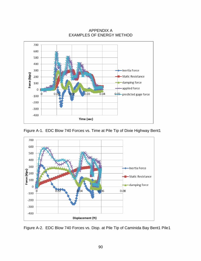
90

APPENDIX A

EXAMPLES OF ENERGY METHOD

Figure A-1. EDC Blow 740 Forces vs. Time at Pile Tip of Dixie Highway Bent1

Figure A-2. EDC Blow 740 Forces vs. Disp. at Pile Tip of Caminida Bay Bent1 Pile1

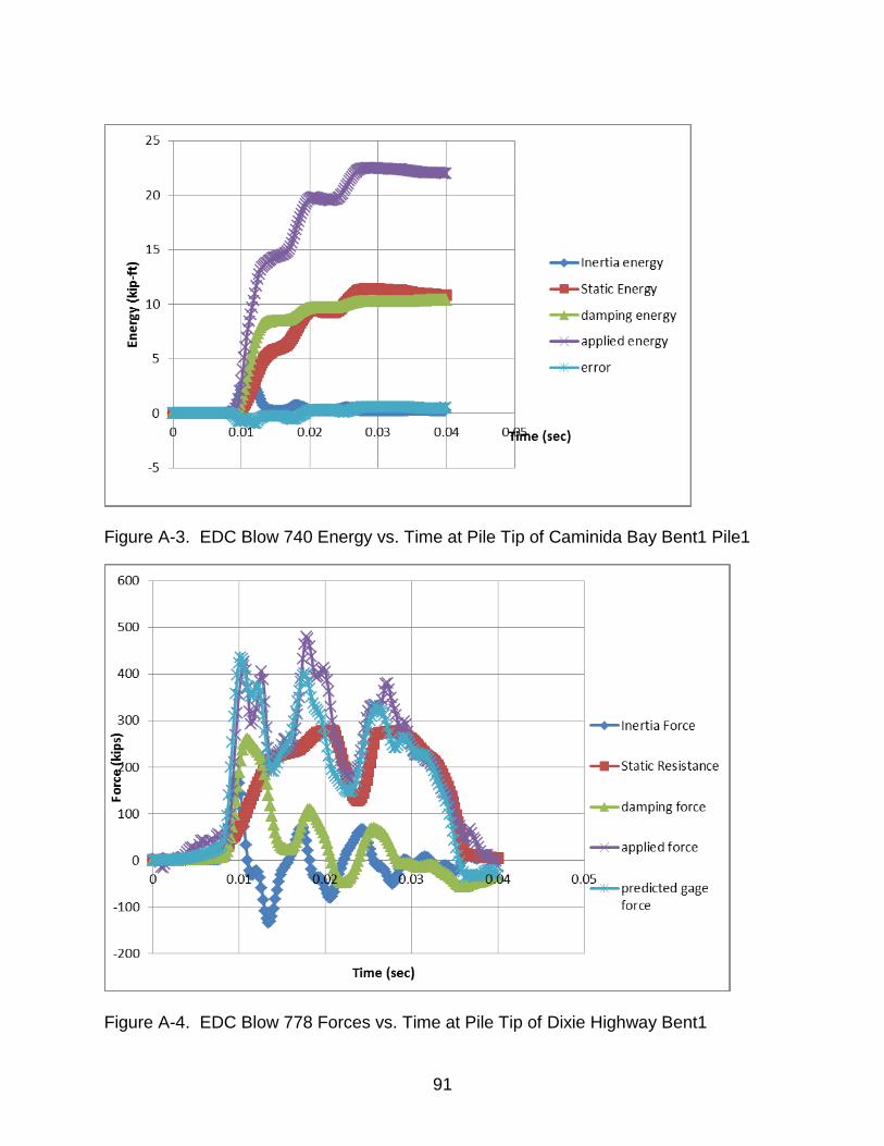
91

Figure A-3. EDC Blow 740 Energy vs. Time at Pile Tip of Caminida Bay Bent1 Pile1

Figure A-4. EDC Blow 778 Forces vs. Time at Pile Tip of Dixie Highway Bent1

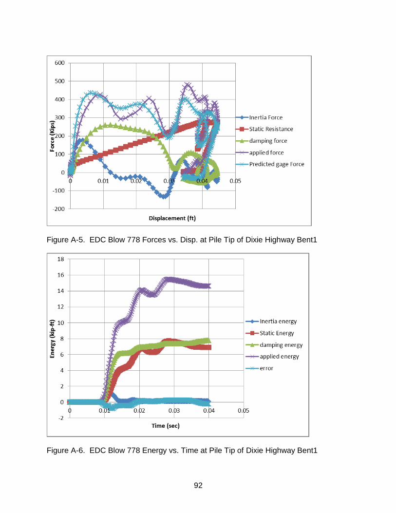
92

Figure A-5. EDC Blow 778 Forces vs. Disp. at Pile Tip of Dixie Highway Bent1

Figure A-6. EDC Blow 778 Energy vs. Time at Pile Tip of Dixie Highway Bent1

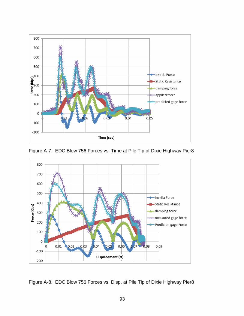
93

Figure A-7. EDC Blow 756 Forces vs. Time at Pile Tip of Dixie Highway Pier8

Figure A-8. EDC Blow 756 Forces vs. Disp. at Pile Tip of Dixie Highway Pier8

94

Figure A-9. EDC Blow 756 Energy vs. Time at Pile Tip of Dixie Highway Pier8

Figure A-10. EDC Blow 779 Forces vs. Time at Pile Tip of Dixie Highway Pier8

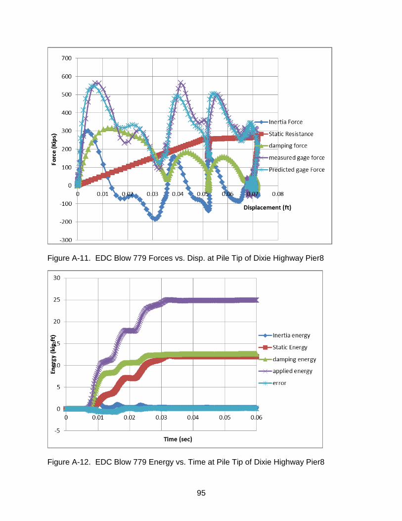
95

Figure A-11. EDC Blow 779 Forces vs. Disp. at Pile Tip of Dixie Highway Pier8

Figure A-12. EDC Blow 779 Energy vs. Time at Pile Tip of Dixie Highway Pier8

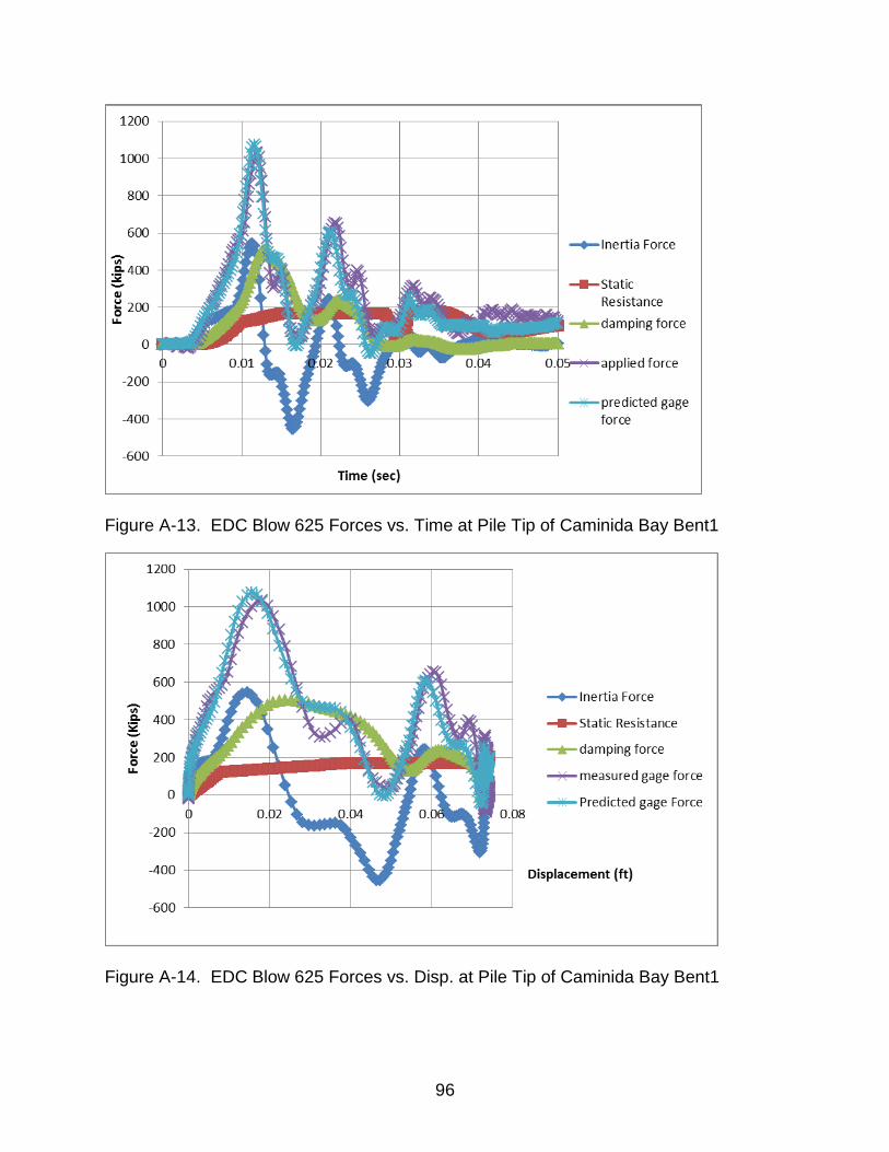
96

Figure A-13. EDC Blow 625 Forces vs. Time at Pile Tip of Caminida Bay Bent1

Figure A-14. EDC Blow 625 Forces vs. Disp. at Pile Tip of Caminida Bay Bent1

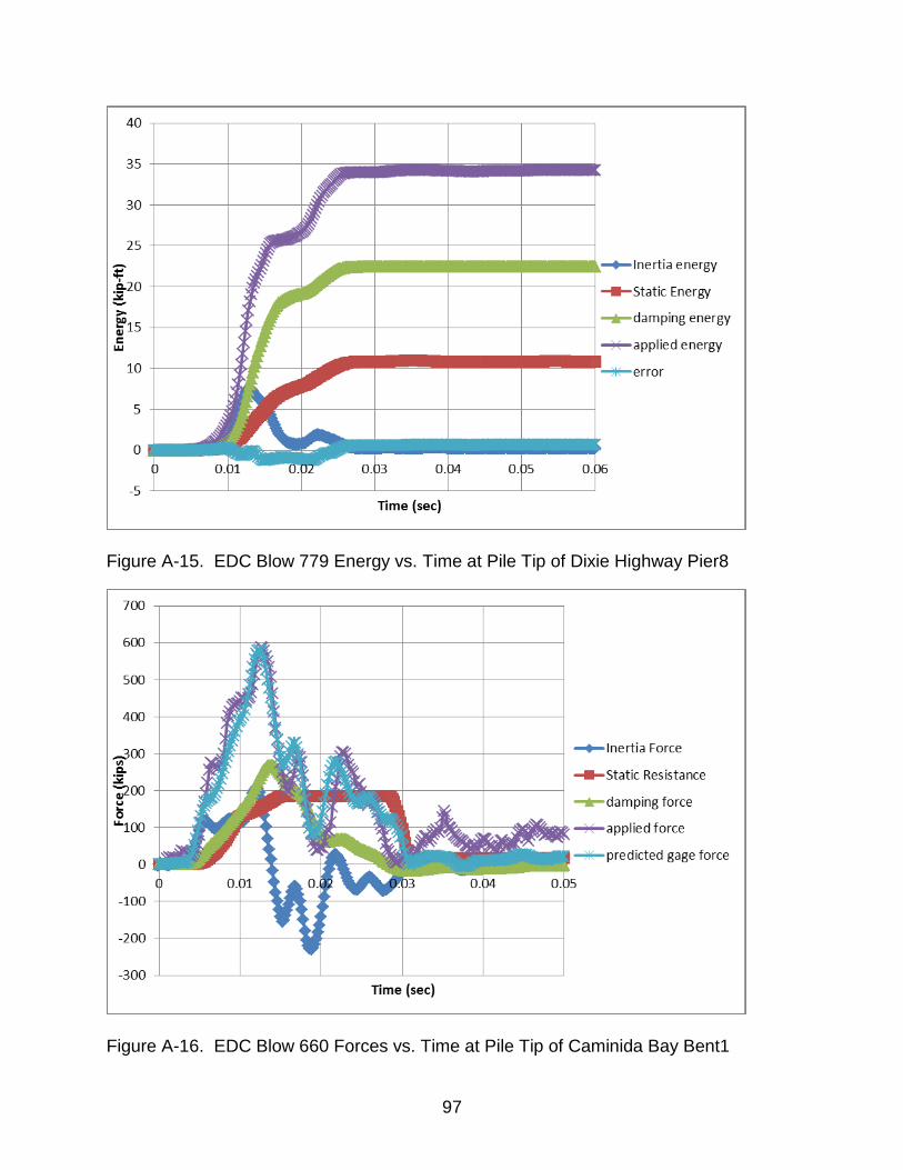
97

Figure A-15. EDC Blow 779 Energy vs. Time at Pile Tip of Dixie Highway Pier8

Figure A-16. EDC Blow 660 Forces vs. Time at Pile Tip of Caminida Bay Bent1

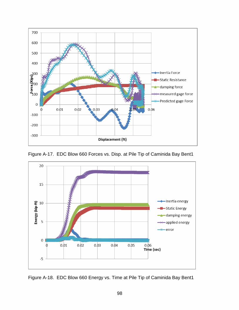
98

Figure A-17. EDC Blow 660 Forces vs. Disp. at Pile Tip of Caminida Bay Bent1

Figure A-18. EDC Blow 660 Energy vs. Time at Pile Tip of Caminida Bay Bent1

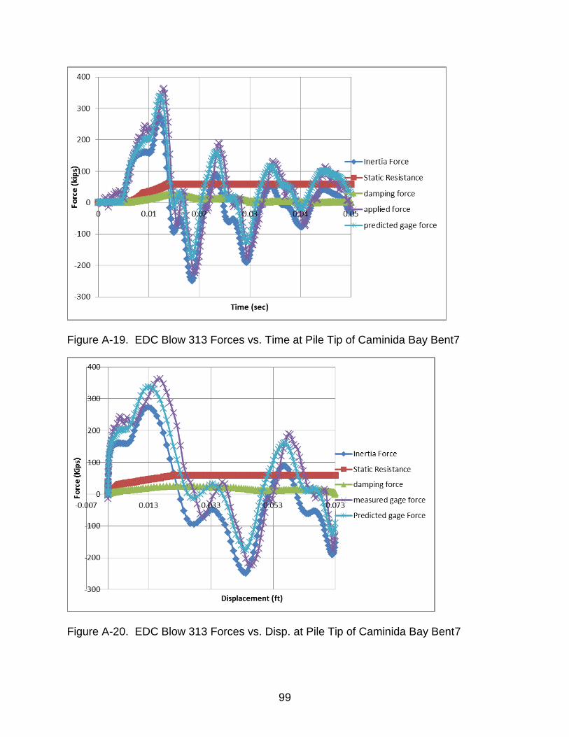
99

Figure A-19. EDC Blow 313 Forces vs. Time at Pile Tip of Caminida Bay Bent7

Figure A-20. EDC Blow 313 Forces vs. Disp. at Pile Tip of Caminida Bay Bent7

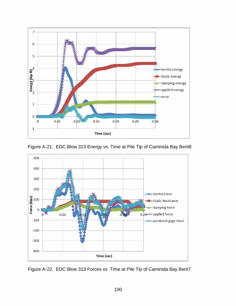
100

Figure A-21. EDC Blow 313 Energy vs. Time at Pile Tip of Caminida Bay Bent8

Figure A-22. EDC Blow 313 Forces vs. Time at Pile Tip of Caminida Bay Bent7

101

Figure A-23. EDC Blow 313 Forces vs. Disp. at Pile Tip of Caminida Bay Bent7

Figure A-24. EDC Blow 313 Energy vs. Time at Pile Tip of Caminida Bay Bent7

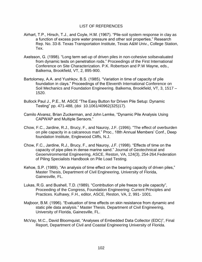
102

LIST OF REFERENCES

Airhart, T.P., Hirsch, T.J., and Coyle, H.M. (1967). “Pile-soil system response in clay as a function of excess pore water pressure and other soil properties.” Research Rep. No. 33-8. Texas Transportation Institute, Texas A&M Univ., College Station, Tex.

Axelsson, G. (1998). “Long term set-up of driven piles in non-cohesive soilsevaluated from dynamic tests on penetration rods.” Proceedings of the First International Conference on Site Characterization. P.K. Robertson and P.W Mayne, eds., Balkema, Brookfield, VT, 2, 895-900.

Bartolomey, A.A. and Yushkov, B.S. (1985). “Variation in time of capacity of pile foundation in clays.” Proceedings of the Eleventh International Conference on Soil Mechanics and Foundation Engineering. Balkema, Brookfield, VT, 3, 1517 – 1520.

Bullock Paul J., P.E., M. ASCE “The Easy Button for Driven Pile Setup: Dynamic Testing” pp. 471-488, (doi 10.1061/40962(325)17).

Camilo Alvarez, Brian Zuckerman, and John Lemke, “Dynamic Pile Analysis Using CAPWAP and Multiple Sensors.”

Chow, F.C., Jardine, R.J., Brucy, F., and Nauroy, J.F. (1996). “The effect of overburden on pile capacity in a calcareous marl.” Proc., 18th Annual Members’ Conf., Deep foundation Institute, Englewood Cliffs, N.J.

Chow, F.C., Jardine, R.J., Brucy, F., and Nauroy, J.F. (1998). “Effects of time on the capacity of pipe piles in dense marine sand.” Journal of Geotechnical and Geoenvironmental Engineering, ASCE, Reston, VA, 124(3), 254-264.Federation of Piling Specialists Handbook on Pile Load Testing.

Kehoe, S.P. (1989). “An analysis of time effect on the bearing capacity of driven piles,” Master Thesis, Department of Civil Engineering, University of Florida, Gainesville, FL.

Lukas, R.G. and Bushell, T.D. (1989). “Contribution of pile freeze to pile capacity”, Proceeding of the Congress, Foundation Engineering: Current Principles and Practices. Kulhawy, F.H., editor, ASCE, Reston, VA, 2, 991- 1001.

Majboor, B.M. (1996). “Evaluation of time effects on skin resistance from dynamic and static pile data analysis.” Master Thesis. Department of Civil Engineering, University of Florida, Gainesville, FL.

McVay, M.C., David Bloomquist, “Analyses of Embedded Data Collector (EDC)”, Final Report, Department of Civil and Coastal Engineering University of Florida.

103

McVay, M.C.,David Bloomquist, “Embedded Data Collector (EDC) Evaluation Phase II” Progress Report 3, Department of Civil and Coastal Engineering University of Florida.

McVay, M.C., Schmertmann, J. and Bullock, P. (1999). “Pile friction freeze: a field and laboratory study.” Research Report submitted to Florida Department of Transportation. Department of Civil Engineering, University of Florida, Gainesville, FL.

Pestana, J.M., Hunt, C.E., and Bray, J.D. (2002). “Soil Deformation and Excess Pore Pressure Field around A Closed-Ended Pile.” Journal of Geotechnical and Geoenvionmental Engineering, ASCE, Vol. 128, No.1, pp.1-12

Randolph, M.F., Carter, J.P., and Wroth, C.P. (1979). “Driven Piles in Clay – the Effects of Installation and Subsequent Consolidation” Geotechnique 29, No.4, pp. 361-393

Samson, L. and Authier, J. (1986). “Change in pile capacity with time: case histories” Canadian Geotechnical Journal. Natiaonal Research Council of Canada, Ottawa, Ontario, 23(2), 174-180.

Schmertmann, J.H. (1981). “A general time-related soil friction increase phenomenon.” American Society for Testing and Materials, Philadelphia, PA, 456-484. Laboratory Shear Strength of soil, ASTM STP 740. Yong, R.N. and Townsend, F.C.

Schmertmann, J.H. (1991). “The mechanical aging of soils (25th Karl Terzaghi lecture).” Journal of Geotechnical Engineering, ASCE, Reston VA 117 (9), 1285-1330.

Seidel, J.P.,Haustorfer,I.J., and Plesiotis, S.(1988). “Comparison of static and dynamic testing for piles founded into limestone.” Proceedings of the Third International Conference on the Application of Stress-Wave Theory to Piles. Fellenius.

Svinkin, M.R., C.M. Morgano & M. Morvant 1994. Pile capacity as a function of time in clayey and sandy soils. Proc. Fifth Inter. Conf. and Exhibition on Piling and Deep Foundations, Bruges, 13-15 June: 1.11.1-1.11.8, Rotterdam: Balkema.

Skov, R., and Denver, H. (1988). “Time-dependence of bearing capacity of piles.” Proceedings of the Third international Conference on the application of Stress-Wave Theory to Piles. Felllenius, B.G., editor, BiTech Publishers, Vancouver, BC, 879-888.

Van E. Komurka , Alan B. Wagner, Wagner Komurka (2003) “Estimating soil/pile set-up” Final Report, (WHRP) by the Wisconsin Department of Transportation (WisDOT) and the Federal Highway Administration (“FHWA”) under Project #0092-00-14.

104

Waldle, I.F., G,Price & T.J.Freeman 1992 “Effect of time and maintained load on the ultimate capacity of piles in stiff clay.” Pilling: European practice and worldwide trends, Proc. Institution of Civil Engineers: 92-99, London: Telford.

W.K.Ng, M.R.Selamat, K.K. Choong, “Soil/Pile Set-up Effects on Driven Pile in Malaysian Soil”, Vol. 14 [2010], Bund. A

York, D.L., Brusey, W.G.,Clemente, F.M., and Law, S.K. (1994). “Setup and relaxation in glacial sands.” Journal of Geotechninal Engineering, ASCE, Reston, VA

105

BIOGRAPHICAL SKETCH

She was born on May 21, 1986. She finished her undergraduate study and got her

B.S. in Hohai University, Nanjing, China. In the August, 2008 She came to America to

pursue her master’s degree in University of Florida, majoring in Geotechnical

Engineering. Here she met her favorite Professor Dr. McVay who she followed to do

research and under his instruction finished this master thesis. She admires his profound

knowledge of geotechnical engineering and pure-hearted character, determine to

become a eligible engineer like him in the future.