numerical realization for analysis of real flows by integrating computation and measurement

INTERNATIONAL JOURNAL FOR NUMERICAL METHODS IN FLUIDSInt. J. Numer. Meth. Fluids 2005; 47:543–559Published online 17 December 2004 in Wiley InterScience (www.interscience.wiley.com). DOI: 10.1002/�d.829

Numerical realization for analysis of real �ows by integratingcomputation and measurement

Toshiyuki Hayase∗;†, Keisuke Nisugi and Atsushi Shirai

Institute of Fluid Science; Tohoku University; Japan

SUMMARY

In this paper, we deal with a numerical realization, which is a numerical analysis methodology toreproduce real �ows by integrating numerical simulation and measurement. It is di�cult to measure orcalculate �eld information of real three-dimensional unsteady �ows due to the lack of an experimental�eld measurement method, as well as of a way to specify the exact boundary or initial conditionsin computation. Based on the observer theory, numerical realization is achieved by a combination ofnumerical simulation, experimental measurement, and a feedback loop to the simulation from the outputsignals of both methods. The present paper focuses on the problem of how an inappropriate model orinsu�cient grid resolution in�uences the performance of the numerical realization in comparison withordinary simulation. For a fundamental �ow with the Karman vortex street behind a square cylinder,two-dimensional analysis is performed by means of numerical realization and ordinary simulation withthree grid resolutions. Comparison of the results with those of the experiment proved that the feedbackof the experimental measurement signi�cantly reduces the error due to insu�cient grid resolution ande�ectively reduces the error due to inappropriate model assuming two-dimensionality. Copyright ? 2004John Wiley & Sons, Ltd.

KEY WORDS: numerical realization; numerical simulation; experiment; feedback; observer; Karmanvortex street

1. INTRODUCTION

Numerical simulation and experiment are essential tools in �ow analysis, but not appropriate toreproduce real �ows exactly. It is apparent that there is no measurement method with whichit is possible to obtain complete information on general time-dependent three-dimensional�ows. This fact also explains why exact simulation is impossible for real �ows whose exactboundary and initial conditions are not available. This paper deals with a numerical analysis

∗Correspondence to: Toshiyuki Hayase, Institute of Fluid Science, Tohoku University, 2-1-1 Katahira, Sendai 980-8577, Japan.

†E-mail: [email protected]

Contract=grant sponsor: Grant-in-aid for Scienti�c Research; contract=grant numbers: 10650157, 11555053

Received 15 August 2003Copyright ? 2004 John Wiley & Sons, Ltd. Accepted 18 August 2004

544 T. HAYASE, K. NISUGI AND A. SHIRAI

Simulation

Error due to B. C. or I. C.

Real flow?

Simulation Real flowOutputsignal

+-Feedback

(a) (b)

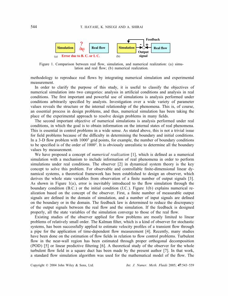
Figure 1. Comparison between real �ow, simulation, and numerical realization: (a) simu-lation and real �ow; (b) numerical realization.

methodology to reproduce real �ows by integrating numerical simulation and experimentalmeasurement.In order to clarify the purpose of this study, it is useful to classify the objectives of

numerical simulation into two categories: analysis in arti�cial conditions and analysis in realconditions. The �rst important and powerful use of simulations is analysis performed underconditions arbitrarily speci�ed by analysts. Investigation over a wide variety of parametervalues reveals the structure or the internal relationship of the phenomena. This is, of course,an essential process in design problems, and thus, numerical simulation has been taking theplace of the experimental approach to resolve design problems in many �elds.The second important objective of numerical simulations is analysis performed under real

conditions, in which the goal is to obtain information on the internal states of real phenomena.This is essential in control problems in a wide sense. As stated above, this is not a trivial issuefor �eld problems because of the di�culty in determining the boundary and initial conditions.In a 3-D �ow problem with 10003 grid points, for example, the number of boundary conditionsto be speci�ed is of the order of 10002. It is obviously unrealistic to determine all the boundaryvalues by measurement.We have proposed a concept of numerical realization [1], which is de�ned as a numerical

simulation with a mechanism to include information of real phenomena in order to performsimulations under real conditions. The observer [2] in dynamical system theory is the keyconcept to solve this problem. For observable and controllable �nite-dimensional linear dy-namical systems, a theoretical framework has been established to design an observer, whichderives the whole state variables from observation of a �nite number of output signals [3].As shown in Figure 1(a), error is inevitably introduced to the �ow simulation through theboundary condition (B.C.) or the initial condition (I.C.). Figure 1(b) explains numerical re-alization based on the concept of the observer. First, a �nite number of measurable outputsignals are de�ned in the domain of simulation, and a number of input signals are de�nedon the boundary or in the domain. The feedback law is determined to reduce the discrepancyof the output signals between the real �ow and the simulation. If the feedback is designedproperly, all the state variables of the simulation converge to those of the real �ow.Existing studies of the observer applied for �ow problems are mostly limited to linear

problems of relatively small order. The Kalman �lter, which is a kind of observer for stochasticsystems, has been successfully applied to estimate velocity pro�les of a transient �ow througha pipe for the application of time-dependent �ow measurement [4]. Recently, many studieshave been done on the estimation of �ow �elds in relation to �ow control problems. Turbulent�ow in the near-wall region has been estimated through proper orthogonal decomposition(POD) [5] or linear predictive �ltering [6]. A theoretical study of the observer for the wholeturbulent �ow �eld in a square duct has been made by the present author [7]. In that work,a standard �ow simulation algorithm was used for the mathematical model of the �ow. The

Copyright ? 2004 John Wiley & Sons, Ltd. Int. J. Numer. Meth. Fluids 2005; 47:543–559

NUMERICAL REALIZATION OF REAL FLOWS 545

feedback controller in the observer was designed to compensate the boundary condition ofthe simulation based on the estimation error between output signals of the computational andthe experimental results, the latter of which is represented by the DNS result. The estimationerror in the axial velocity at the grid points on a cross-section is fed back to the pressureboundary condition based on the simple proportional control law. Appropriate choice of thefeedback gain signi�cantly accelerates the convergence of the iterative calculation and reducesthe error in the downstream region of the output measurement plane. As the �rst case ofintegration of computation and experiment in a real system, the hybrid wind tunnel wasconstructed by integrating an experimental wind tunnel and a supercomputer through a highspeed network [8]. Numerical realization was carried out with this equipment for the �ow withthe Karman vortex street behind a square cylinder. Pressure measurement on the cylinder wallwas fed back to the numerical simulation showing that the numerical realization reproduces theKarman vortex appearing in a real �ow. Especially, exact synchronization of the oscillationsobtained by computation and experiment is a speci�c feature of the hybrid wind tunnel.As the potential of the above-mentioned numerical realization method in simulating real

�ows has been ascertained, fundamental properties of the methodology should be further in-vestigated. The present paper focuses on the problem of how an inappropriate model and insuf-�cient grid resolution in�uence the performance of the present numerical realization method.It is common to begin a numerical analysis in a rather restricted but simple condition, suchas an assumption of two-dimensionality of a relevant �ow. The question to be investigated iswhether the feedback of measurement data in the numerical realization can reduce the e�ectof the model error in comparison with ordinary simulations. The second question is whetherthe e�ect of incomplete grid resolution can be reduced by the feedback action. In order toinvestigate these problems, numerical realization and ordinary simulation are performed withthree grid systems of di�erent resolutions, and all the results, including the experimental one,are compared with each other.In Section 2 of the paper, the governing equations and numerical procedures for computation

of the 2-D channel �ow with a square object are presented. Inclusion of the measurement inthe computation is explained in detail. In Section 3, results for the �ow with the Karman vortexstreet are compared between the numerical realization, the ordinary numerical simulation forthree grid resolutions and the experiment. Section 4 of the paper presents the conclusions ofthe work.

2. FORMULATION

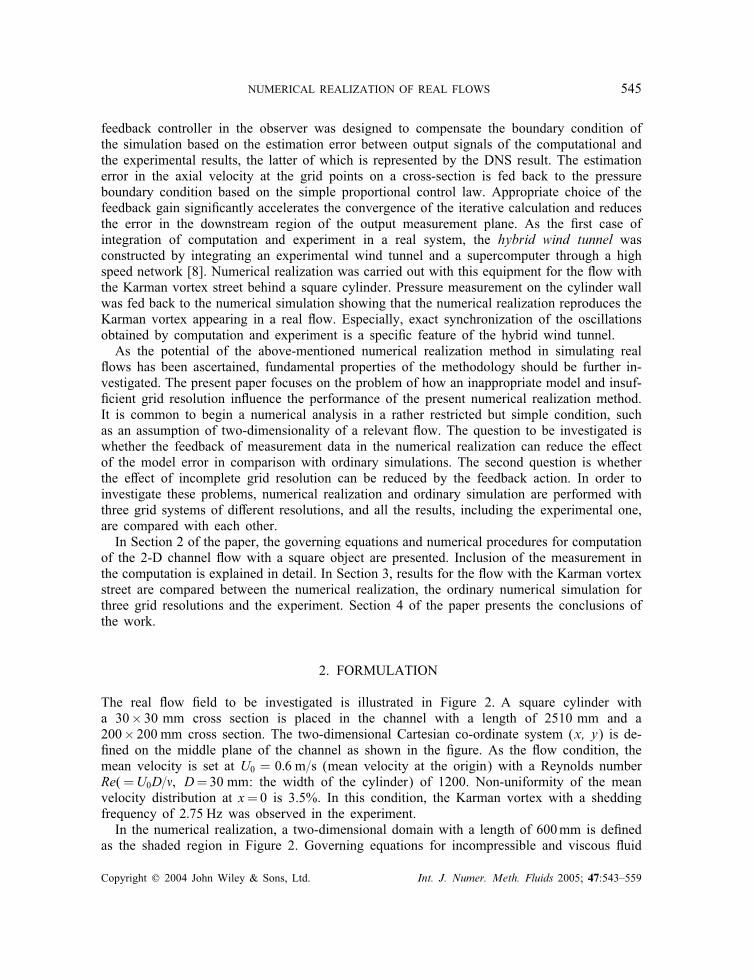
The real �ow �eld to be investigated is illustrated in Figure 2. A square cylinder witha 30× 30 mm cross section is placed in the channel with a length of 2510 mm and a200× 200 mm cross section. The two-dimensional Cartesian co-ordinate system (x, y) is de-�ned on the middle plane of the channel as shown in the �gure. As the �ow condition, themean velocity is set at U0 = 0:6 m=s (mean velocity at the origin) with a Reynolds numberRe(=U0D=�; D=30 mm: the width of the cylinder) of 1200. Non-uniformity of the meanvelocity distribution at x=0 is 3.5%. In this condition, the Karman vortex with a sheddingfrequency of 2:75 Hz was observed in the experiment.In the numerical realization, a two-dimensional domain with a length of 600mm is de�ned

as the shaded region in Figure 2. Governing equations for incompressible and viscous �uid



y

x30

30M

o

120

200 x 200

(mm)

2510

205 90 500

Suction

Mid plane

60

50

Figure 2. Geometry and coordinate system.

�ow are the Navier–Stokes equation

�(@u@t+ (u · grad)u

)=−grad P + �∇2u+ f (1)

and the equation of continuity

divu=0 (2)

where f in Equation (1) is the arti�cial body force corresponding to the feedback signal in thenumerical realization as described later in this section. Parallel �ow with the uniform velocityUb is applied at the upstream boundary,

u(y)=Ub; v(y)=0 at x=−D=3 (3)

where the upstream boundary velocity Ub is treated as the feed-forward input variable inthe numerical realization. The downstream boundary condition is free stream. The no-slipcondition is applied on the solid walls. All velocity components are initially set at null in thewhole domain.The governing equations are discretized with the �nite volume method on the uniformly

spaced staggered grid system and are solved with the algorithm similar to the SIMPLERmethod of Patankar [9]. As the main feature of the present scheme, (1) a consistently re-formulated QUICK scheme is applied to the convective terms [10] and (2) the second orderimplicit scheme is used for the time derivative terms [11]. Details of the scheme are givenin a previous paper [12].Three grid systems of di�erent resolutions, i.e. Nx ×Ny=60× 21 (Grid A), 120×

42 (Grid B), and 240× 82 (Grid C), are used for the numerical realization and the ordinarysimulation. A time step of 1ms, the same as the sampling time of the pressure measurement,was con�rmed to be su�ciently small for the present calculations. Conditions used in thecalculation are summarized in Table I.In the numerical realization, measurement of the real �ow is supplied to the numerical

simulation to compensate for the di�erences between the real �ow and the computation.Since we focus on the Karman vortex originating from the cylinder, the output signal to bemeasured is de�ned as the pressure on the both sides of the cylinder relative to the stagnationpressure (see Figure 3), (

P∗AS

P∗BS

)=

(P∗A − P∗

S

P∗B − P∗

S

)(4)



Table I. Computational condition.

Grid system Grid A Grid B Grid C

Domain Lx × Ly 20D× 6:67DGrid points Nx ×Ny 60× 21 120× 42 240× 82Grid spacing hx × hy D=3×D=3 D=6×D=6 D=12×D=12Time step ht 0:001 sWidth of cylinder D 0:03 mMean velocity U0 0:6 m=sReynolds number Re 1200

fBB

fA

Ps

S

PA*

PB*

PS*

AUb

Grid C Grid B

Grid A

fA

PA

Upstreamboundary

Figure 3. Details of the square cylinder.

where the asterisk represents experimental values. Corresponding variables PAS and PBS arede�ned using the computational results. Note that the location of pressure evaluation in thecomputation is di�erent between the grid systems as shown in Figure 3.The arti�cial body force f in Equation (1) is calculated in proportion to the di�erence

between the output signals in the experiment and those in the calculation. The correspondingforces fA and fB are applied to the control volumes A and B (Figure 3), respectively, in thex-direction momentum equation.(

fA

fB

)=−KAC

(PAS − P∗

AS

PBS − P∗BS

)(5)

where K denotes the feedback gain (non-dimensional), and AC the cross-sectional area ofthe control volume. The velocity component u is accelerated or decelerated by the feedbackof Equation (5) at the upstream boundary of the pressure control volumes. As a result, thepressure error in the pressure equation decreases in these control volumes.The uniform �ow velocity of the real �ow is estimated from the pressure measurement

with the Pitot tube law [13], and fed forward to the upstream boundary velocity Ub of thesimulation through the �rst-order low pass �lter as

TcdUbdt

+Ub =Ke

√2P∗

m

�(6)



Real flow

Velocity estimation

Numerical analysis

Feedback law

B.C.

B.C.

Ub

PAS* , PBS

*

PAS , PBS

-

+Pm

*

Pressure on side wall(measurement)

Pressure on side wall(calculation)

ErrorArtificialforce

Upstream boundary velocity

fA

fB

PAS-PAS*

PBS-PBS*

Figure 4. Block diagram of numerical realization for Karman vortex.

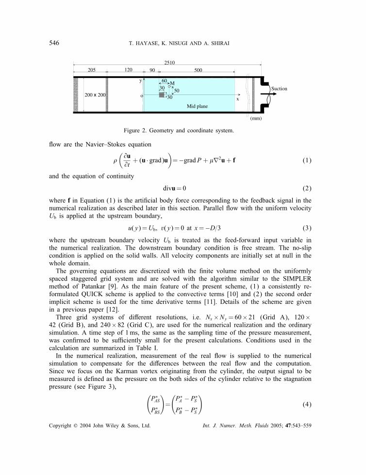
where Tc is the time constant of the �lter, Ke is the velocity coe�cient (non-dimensional),and P∗

m is the dynamic pressure estimated as

P∗m =−P

∗AS + P

∗BS

2=P∗

S − P∗A + P

∗B

2(7)

Figure 4 shows the block diagram of the numerical realization. The pressure error on bothsidewalls is fed back to the arti�cial forces fA and fB, and the estimated uniform �ow velocityUb is fed forward to the upstream boundary velocity condition.

3. RESULTS AND DISCUSSION

Three parameters in designing the numerical realization, namely, the feedback gain K , thevelocity coe�cient Ke, and the time constant Tc, are so determined that the estimated velocityu at the monitoring point M ((x; y)= (5D; 1:67D), see Figure 2) best agrees with that of theexperiment. The results are given as

K =1:8; Ke=

0:54 (grid A)

0:56 (grid B);

0:60 (grid C)

Tc=0:3 [s] (8)

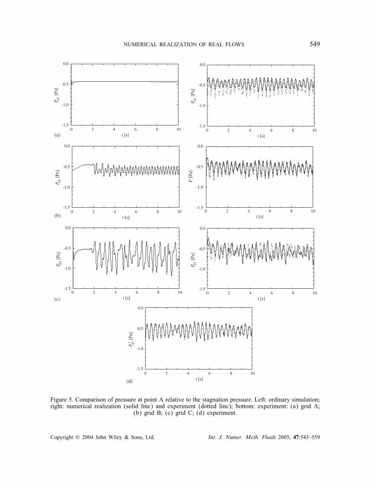
It is noted that only the parameter Ke depends on the grid system since the computationalresult is very sensitive to this parameter in comparison with the other parameters [8].The results for one of the output signals, i.e. PAS , the pressure at point A on the sidewall

relative to the stagnation pressure, are compared in Figure 5. In Figures (a)–(c) correspondingto grids A–C, the left-hand side shows the results of the ordinary simulation and the right-hand side shows those of the numerical realization. Figure 5(d) shows the experimental result.



0 2 4 6 8 10-1.5

-1.0

-0.5

0.0

P AS [

Pa]

-1.5

-1.0

-0.5

0.0

P AS [

Pa]

-1.5

-1.0

-0.5

0.0

P [

Pa]

-1.5

-1.0

-0.5

0.0

P AS [

Pa]

-1.5

-1.0

-0.5

0.0

P AS [

Pa]

-1.5

-1.0

-0.5

0.0

P AS [

Pa]

-1.5

-1.0

-0.5

0.0

P AS* [

Pa]

t [s]0 2 4 6 8 10

t [s]

0 2 4 6 8 10t [s]

0 2 4 6 8 10t [s]

0 2 4 6 8 10t [s]

0 2 4 6 8 10t [s]

0 2 4 6 8 10t [s]

(a)

(b)

(c)

(d)

Figure 5. Comparison of pressure at point A relative to the stagnation pressure. Left: ordinary simulation;right: numerical realization (solid line) and experiment (dotted line); bottom: experiment: (a) grid A;

(b) grid B; (c) grid C; (d) experiment.



The ordinary simulation on the left-hand side shows a variety of results, but none of theseresembles the experimental result. With the coarse grid A, oscillation is almost invisible. Theresult of grid B shows a sinusoidal oscillation after the transient, and that of the �ne grid Cshows an irregular oscillation of large amplitude. It is noted that the result of the ordinarysimulation with grid C is almost convergent with the grid re�nement, which is con�rmed bycomparison with the result for the grid system which is twice as �ne. In contrast, results of thenumerical realization on the right-hand side show far better agreement with the experimentalresults (dotted lines, identical to Figure 5(d)) than do the results of the ordinary simulations.This justi�es the appropriateness of the feedback algorithm de�ned in the former section forreducing the discrepancy of the pressure at points A and B.A feedback signal for the numerical realization, or the arti�cial force applied to control

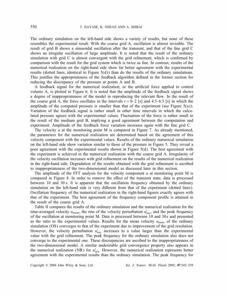
volume A, is plotted in Figure 6. It is noted that the amplitude of the feedback signal showsa degree of inappropriateness of the model in reproducing the relevant �ow. In the result ofthe coarse grid A, the force oscillates in the intervals t=0–2 [s] and 4.5–6.5 [s] in which theamplitude of the computed pressure is smaller than that of the experiment (see Figure 5(a)).Variation of the feedback signal is rather small in other time intervals in which the calcu-lated pressure agrees with the experimental values. Fluctuation of the force is rather small inthe result of the medium grid B, implying a good agreement between the computation andexperiment. Amplitude of the feedback force variation increases again with the �ne grid C.The velocity u at the monitoring point M is compared in Figure 7. As already mentioned,

the parameters for the numerical realization are determined based on the agreement of thisvelocity component with the experimental values. Results of the ordinary numerical simulationon the left-hand side show variation similar to those of the pressure in Figure 5. They reveal apoor agreement with the experimental results shown in Figure 5(d). The best agreement withthe experiment is achieved in the numerical realization with the coarse grid A. Irregularity ofthe velocity oscillation increases with grid re�nement on the results of the numerical realizationin the right-hand side. Degradation of the results obtained with the grid re�nement is ascribedto inappropriateness of the two-dimensional model as discussed later in this section.The amplitude of the FFT analysis for the velocity component u at monitoring point M is

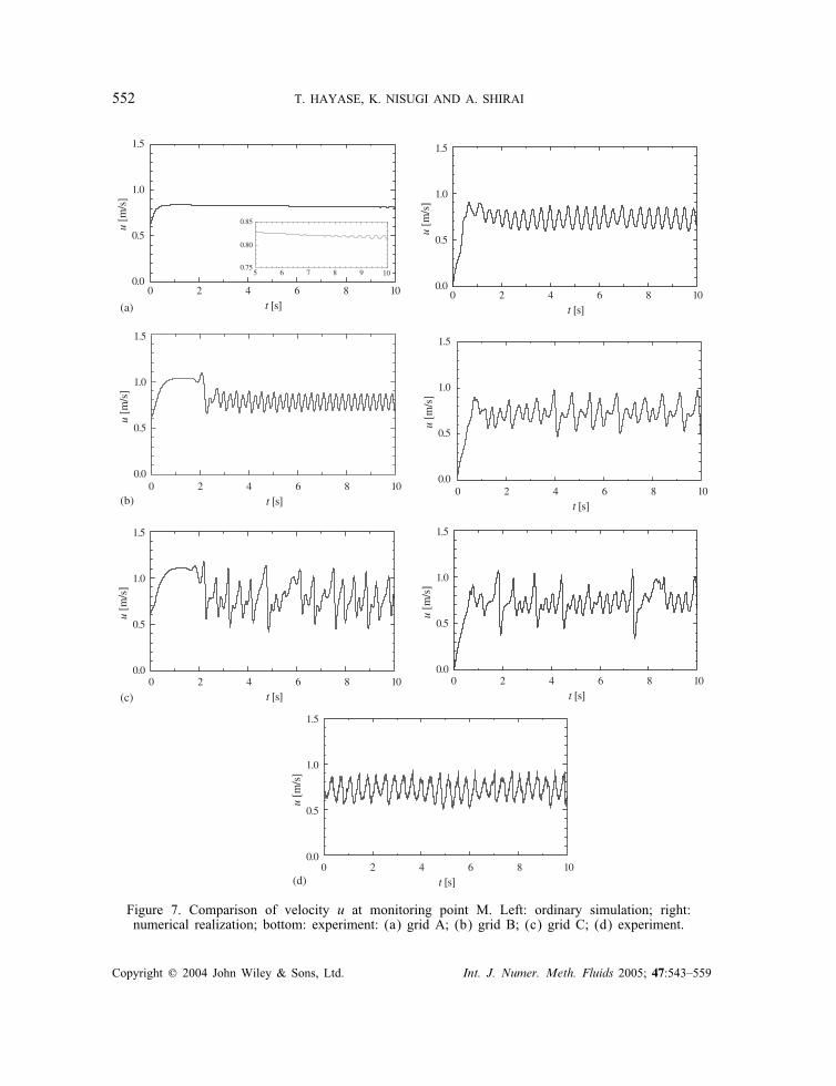
compared in Figure 8. In order to remove the e�ect of the transient state, data is processedbetween 10 and 30 s. It is apparent that the oscillation frequency obtained by the ordinarysimulation on the left-hand side is very di�erent from that of the experiment (dotted lines).Oscillation frequency of the numerical realization in the right-hand �gures exactly agrees withthat of the experiment. The best agreement of the frequency component pro�le is attained inthe result of the coarse grid A.Table II compares the results of the ordinary simulation and the numerical realization for the

time-averaged velocity umean, the rms of the velocity perturbation u′rms, and the peak frequency

of the oscillation at monitoring point M. Data is processed between 10 and 30s and presentedas the ratio to the experimental values. Results for the mean velocity umean of the ordinarysimulation (OS) converges to that of the experiment due to improvement of the grid resolution.However, the velocity perturbation u′

rms increases to a value larger than the experimentalvalue with the grid re�nement. The peak frequency for the ordinary simulation also does notconverge to the experimental one. These discrepancies are ascribed to the inappropriateness ofthe two-dimensional model. A similar undesirable grid convergence property also appears inthe numerical realization (NR) for u′

rms. However, the numerical realization represents betteragreement with the experimental results than the ordinary simulation. The peak frequency for



0 2 4 6 8 10-0.005

-0.004

-0.003

-0.002

-0.001

0.000

0.001

0.002

0.003

0.004

0.005

t [s]

f A [N

]

0 2 4 6 8 10-0.005

-0.004

-0.003

-0.002

-0.001

0.000

0.001

0.002

0.003

0.004

0.005

t [s]

f A [N

]

0 2 4 6 8 10-0.005

-0.004

-0.003

-0.002

-0.001

0.000

0.001

0.002

0.003

0.004

0.005

t [s]

f A [N

]

(a)

(b)

(c)

Figure 6. Force applied at point A in numerical realization: (a) grid A; (b) grid B; (c) grid C.

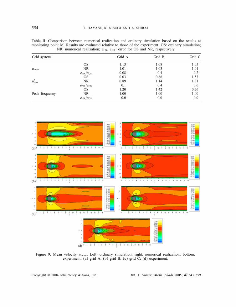
the numerical realization, on the other hand, exactly agrees with that of the experiment forall three grid systems. These results mean that the error introduced by an inappropriate modelis e�ectively reduced by the feedback incorporated in numerical realization.Distributions of the mean velocity umean are compared in Figure 9. Results of the or-

dinary simulation are given on the left-hand side. A stretched wake behind the cylinderin the result of the coarse grid A is much improved in the results of grids B and C,showing good agreement with that of the experiment (Figure (d)). Results of the numeri-cal realization on the right-hand side agree with those of the experiment even with coarsegrid A.



0 2 4 6 8 100.0

0.5

1.0

1.5

u [m

/s]

0.0

0.5

1.0

1.5

u [m

/s]

0.0

0.5

1.0

1.5

u [m

/s]

0.0

0.5

1.0

1.5

u [m

/s]

0.0

0.5

1.0

1.5

u [m

/s]

0.0

0.5

1.0

1.5

u [m

/s]

0.0

0.5

1.0

1.5

u [m

/s]

t [s]0 2 4 6 8 10

t [s]

0 2 4 6 8 10

t [s]

0 2 4 6 8 10

t [s]

0 2 4 6 8 10

t [s]0 2 4 6 8 10

t [s]

0 2 4 6 8 10

t [s]

1098765

0.80

0.85

0.75

(a)

(b)

(d)

(c)

Figure 7. Comparison of velocity u at monitoring point M. Left: ordinary simulation; right:numerical realization; bottom: experiment: (a) grid A; (b) grid B; (c) grid C; (d) experiment.



11 100.00

0.05

0.10

0.15

0.20

Frequency (Hz)

Am

plitu

de

1 100.00

0.05

0.10

0.15

0.20

Frequency (Hz)

Am

plitu

de

1 100.00

0.05

0.10

0.15

0.20

Frequency (Hz)

Am

plitu

de

1 100.00

0.05

0.10

0.15

0.20

Frequency (Hz)

Am

plitu

de

1 100.00

0.05

0.10

0.15

0.20

Frequency (Hz)

Am

plitu

de

1 100.00

0.05

0.10

0.15

0.20

Frequency(Hz)

Am

plitu

de

1 100.00

0.05

0.10

0.15

0.20

Frequency (Hz)

Am

plitu

de

Peak frequencyof experiment

(a)

(b)

(c)

(d)

Figure 8. Comparison of FFT analysis for velocity u at monitoring point M.Left: ordinary simulation; right: numerical realization; bottom: experiment:

(a) grid A; (b) grid B; (c) grid C; (d) experiment.

The rms values of the perturbation velocity u′rms are compared in Figure 10. The result of

the experiment in Figure 10(d) shows large velocity perturbation due to the Karman vortexshedding behind downstream corners of the cylinder. Results of the ordinary simulation onthe left-hand side show a variety of distributions. The coarse grid A does not reproduce



Table II. Comparison between numerical realization and ordinary simulation based on the results atmonitoring point M. Results are evaluated relative to those of the experiment. OS: ordinary simulation;

NR: numerical realization; eOS, eNR: error for OS and NR, respectively.

Grid system Grid A Grid B Grid C

OS 1.13 1.08 1.05umean NR 1.01 1.03 1.01

eNR=eOS 0.08 0.4 0.2OS 0.03 0.66 1.53

u′rms NR 0.89 1.14 1.31

eNR=eOS 0.1 0.4 0.6OS 1.20 1.42 0.76

Peak frequency NR 1.00 1.00 1.00eNR=eOS 0.0 0.0 0.0

Figure 9. Mean velocity umean. Left: ordinary simulation; right: numerical realization; bottom:experiment: (a) grid A; (b) grid B; (c) grid C; (d) experiment.



Figure 10. Perturbation velocity u′rms. Left: ordinary simulation; right: numerical realization;

bottom: experiment: (a) grid A; (b) grid B; (c) grid C; (d) experiment.

the velocity �uctuation near the cylinder but shows a region with small perturbation fardownstream of the cylinder. The result of the moderate grid B shows the best agreementwith the experimental result among the results of the ordinary simulation. The �ne grid Cresults in a much larger amplitude of velocity �uctuation than the experiment. The numericalrealization shows better results than the ordinary simulation for all grid systems. Similar tothe mean velocity distribution, the most signi�cant improvement of the perturbation velocityis seen for the results with the coarse grid A.Reproducibility with the ordinary simulations and the numerical realizations mentioned

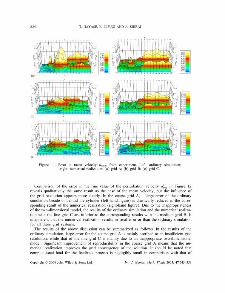
above is quanti�ed by the error with respect to the experiment. Figure 11 compares thedistributions of the error for the mean velocity umean. In the result of the ordinary simulationwith the coarse grid A on the left-hand side of Figure 11(a), a large error occurs behind thecylinder. The result of the numerical realization with the same grid on the right-hand sidereveals a substantial reduction of the error behind the cylinder but some increase near thewalls in the downstream region. The same trend is seen for the other two grids, grids B andC, but the di�erence between the ordinary simulation and the numerical realization is smallerthan in the case of the coarse grid A.



Figure 11. Error in mean velocity umean from experiment. Left: ordinary simulation;right: numerical realization: (a) grid A; (b) grid B; (c) grid C.

Comparison of the error in the rms value of the perturbation velocity u′rms in Figure 12

reveals qualitatively the same result as the case of the mean velocity, but the in�uence ofthe grid resolution appears more clearly. In the coarse grid A, a large error of the ordinarysimulation beside or behind the cylinder (left-hand �gure) is drastically reduced in the corre-sponding result of the numerical realization (right-hand �gure). Due to the inappropriatenessof the two-dimensional model, the results of the ordinary simulation and the numerical realiza-tion with the �ne grid C are inferior to the corresponding results with the medium grid B. Itis apparent that the numerical realization results in smaller error than the ordinary simulationfor all three grid systems.The results of the above discussion can be summarized as follows. In the results of the

ordinary simulation, large error for the coarse grid A is mainly ascribed to an insu�cient gridresolution, while that of the �ne grid C is mainly due to an inappropriate two-dimensionalmodel. Signi�cant improvement of reproducibility in the coarse grid A means that the nu-merical realization improves the grid convergence of the solution. It should be noted thatcomputational load for the feedback process is negligibly small in comparison with that of



Figure 12. Error in perturbation velocity u′rms from experiment. Left: ordinary simulation;

right: numerical realization: (a) grid A; (b) grid B; (c) grid C.

the �ow solver. Reduction of the error for the �ne grid C, on the other hand, means thatnumerical realization also reduces the in�uence of an inappropriate model.Finally, Figure 13 shows some examples of the streakline pattern obtained with the exper-

iment, the numerical realization with the coarse grid A, and the ordinary simulations withthe coarse grid A and the �ne grid C. The streakline pattern of the numerical realization inFigure 13(b) is very similar to that of the experiment in Figure 13(a). It is noted that theoscillation phase of the numerical realization exactly agrees with that of the experiment dueto the feedback e�ect. The streakline pattern of the ordinary simulations with the coarse and�ne grids in Figures 13(c) and (d) both show poor results with smaller or larger �uctuationof the streaklines in comparison with the experiment.

4. CONCLUSIONS

This study constitutes a fundamental study on numerical realization, which is a numericalanalysis methodology to reproduce real �ows by integrating numerical simulation and mea-



Figure 13. Comparison of streakline patterns. t=17:93 s: (a) experiment; (b) numerical realization(grid A); (c) ordinary simulation (grid A); (d) ordinary simulation (grid C).

surement. For a fundamental �ow with the Karman vortex street behind a square cylinder,numerical realization is achieved by a combination of numerical simulation, experimental mea-surement, and a feedback loop to the simulation from the output signals of both the methods.Especially, focus of this study was on the in�uences of an inappropriate model and an in-su�cient grid resolution on the performance of the numerical realization in comparison withthe ordinary simulation. Two-dimensional analysis was performed with three grid systems fornumerical realization and ordinary simulation. Because of the inappropriateness of the two-dimensional model, results of the ordinary simulation for the frequency and the amplitudeof the velocity �uctuation did not converge to those of the experiment. Comparison of thesimulation results with those of the experiment proved that the feedback of the experimentalmeasurement signi�cantly reduces the error due to the insu�cient grid resolution in the coarsegrid and e�ectively reduces the error in the �ne grid due to the inappropriate model.

ACKNOWLEDGEMENTS

The authors express their sincere thanks to technicians T. Hamaya, T. Watanabe, Y. Fushimi, and K.Asano of the Institute of Fluid Science, Tohoku University for construction of the experimental apparatusand graduate student S. Takeda for his patient experimental measurement. The authors also gratefullyacknowledge support received from a Grant-in-aid for Scienti�c Research (#10650157, 11555053). Thecalculations were performed using SGI ORIGIN 2000 at the Advanced Fluid Information ResearchCenter, Institute of Fluid Science, Tohoku University.



REFERENCES

1. Hayase T, Nisugi K, Shirai A. Numerical realization of �ow �eld by integrating computation and measurement.In Proceedings of Fifth World Congress on Computational Mechanics (WCCM V), Mang HA, RammerstorferFG, Eberhardsteiner J (eds). Paper-ID: 81524, 2002; 1–12.

2. Luenberger DG. Introduction to Dynamic Systems: Theory, Models, and Applications. Wiley: New York,1979.

3. Misawa EA, Hedrick JK. Nonlinear observers: a state-of-the-art survey. Journal of Dynamic Systems,Measurement, and Control Transactions (ASME) 1989; 111:344–352.

4. Uchiyama M, Hakomori K. Measurement of Instantaneous �ow rate through estimation of velocity pro�les.IEEE Transaction of Automatic Control 1983; AC-28:380–388.

5. Podvin B, Lumley J. Reconstructing the �ow in the wall region from wall sensors. Physics of Fluids 1998;10:1182–1190.

6. Amonlirdviman K, Breuer K. Linear predictive �ltering in a numerically simulated turbulent �ow. Physics ofFluids 2000; 12:3221–3228.

7. Hayase T, Hayashi S. State estimator of �ow as an integrated computational method with feedback of onlineexperimental measurement. Journal of Fluids Engineering Transactions (ASME) 1997; 119:814–822.

8. Nisugi K, Hayase T, Shirai A. Fundamental study of hybrid wind tunnel integrating numerical simulation andexperiment in analysis of �ow �eld. JSME International Journal 2004; B-47:593–604.

9. Patankar SV. Numerical Heat Transfer and Fluid Flow. Hemisphere: Washington, DC, New York, 1980.10. Hayase T, Humphrey JAC, Greif R. A consistently formulated QUICK scheme for fast and stable convergence

using �nite-volume iterative calculation procedures. Journal of Computational Physics 1992; 98:108–118.11. Fletcher CAJ. Computational Techniques for Fluid Dynamics, vol. 1. Springer: Berlin, 1988; 302.12. Hayase T. Monotonic convergence property of turbulent �ow solution with central di�erence and QUICK

scheme. Journal of Fluids Engineering Transactions (ASME) 1999; 121:351–358.13. Benedict RP. Fundamentals of Pipe Flow. Wiley: New York, 1980.


numerical realization for analysis of real flows by integrating computation and measurement

Documents