computation of free-surface flows using finite-volume...
TRANSCRIPT

Computation of Free-Surface FlowsUsing Finite-Volume Method
Milovan Perić
CD-adapco

Contents
● Finite-volume method
● Moving grids
● Interface-tracking methods for free-surface flows
● Interface-capturing methods for free-surface flows
● Examples of application

Conservation Equations, I
● Conservation equations for space, mass, momentum, and scalars (for an arbitrary moving control volume):

Conservation Equations, II
● For Newtonian fluids, the viscous stress tensor is defined by the Stoke's law:
● In the case of turbulent flows, eddy viscosity models are most often used – the effect of turbulence on the mean flow field is accounted by replacing µ with µ + µturb...
● Turbulent viscosity is a field function obtained from turbulent kinetic energy (velocity scale) and another scalar variable (representing length scale)...
● It can vary by 3 orders of magnitude within the flow field...
Finite-Volume Method, I
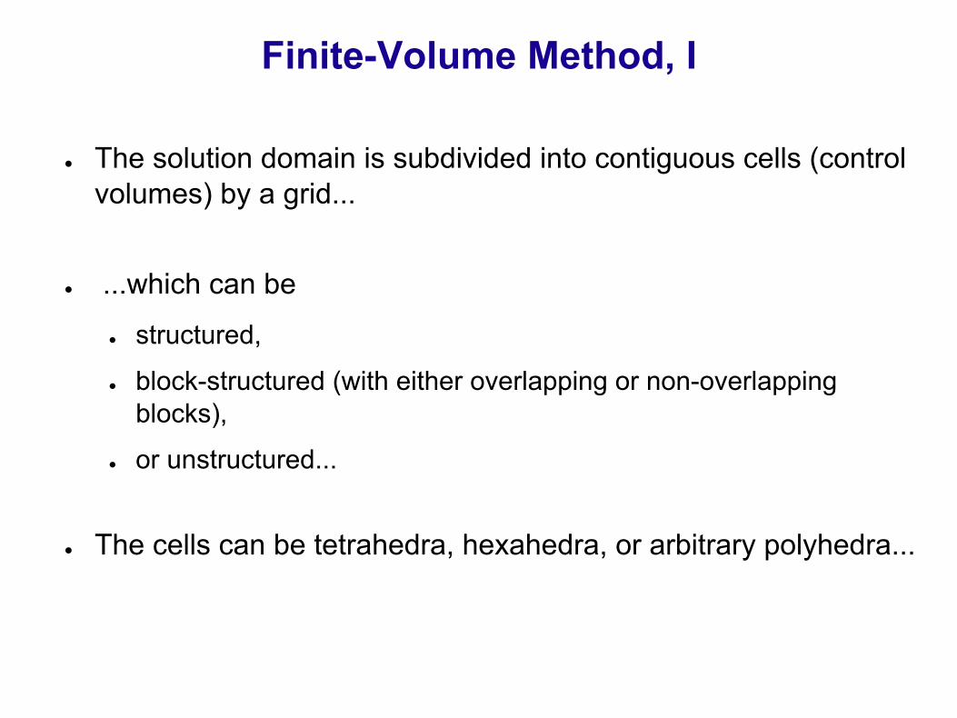
● The solution domain is subdivided into contiguous cells (controlvolumes) by a grid...
● ...which can be
● structured,
● block-structured (with either overlapping or non-overlapping blocks),
● or unstructured...
● The cells can be tetrahedra, hexahedra, or arbitrary polyhedra...

Finite-Volume Methods, II
A block-structured,matching grid
A block-structured,overlapping grid

Finite-Volume Methods, III
A block-structured, non-matching grid

Finite-Volume Methods, IV
An unstructured grid, made of tetrahedra and prism layer along walls

Finite-Volume Methods, V
An unstructured trimmed grid, made of hexahedra, prism layers along walls, and some polyhedra

Finite-Volume Methods, VI
An unstructured grid, made of polyhedra, with prism layers along walls (polygonal prism base)
Polyhedral Control Volumes
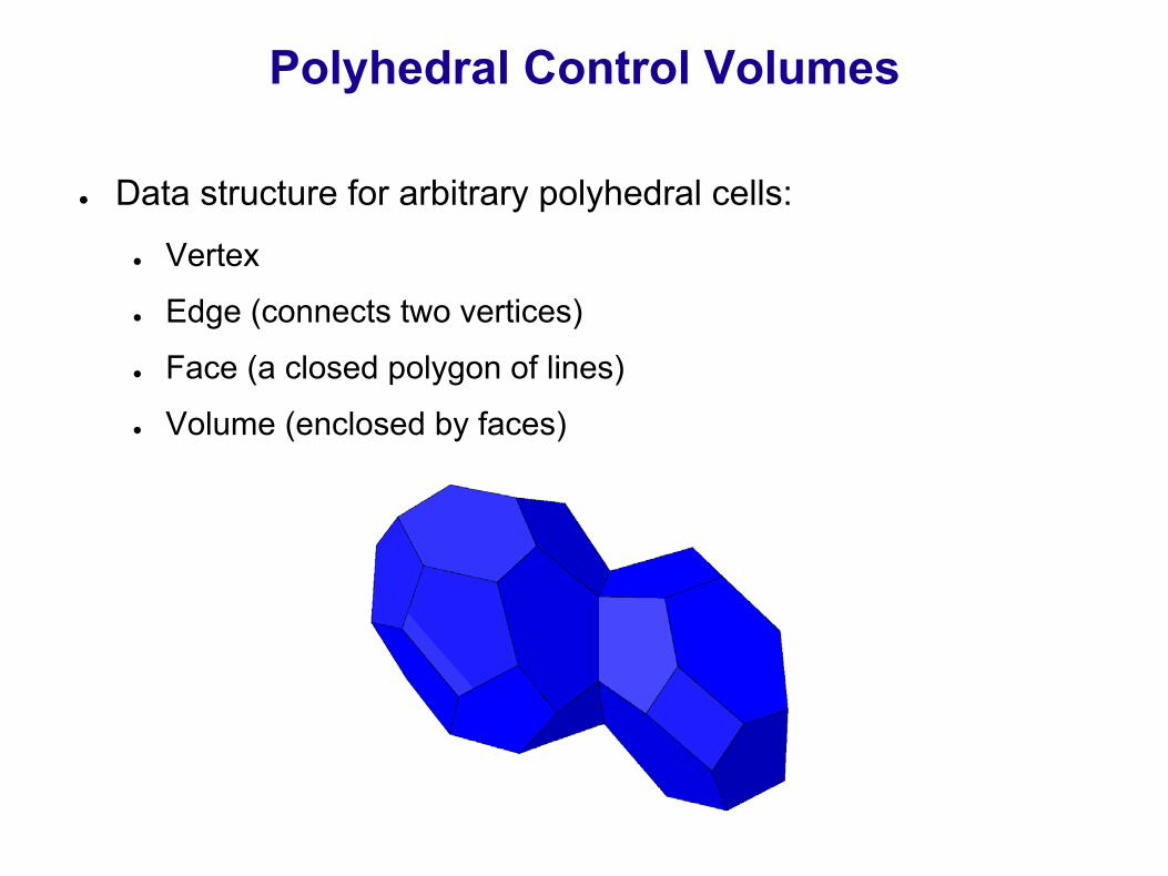
● Data structure for arbitrary polyhedral cells:
● Vertex
● Edge (connects two vertices)
● Face (a closed polygon of lines)
● Volume (enclosed by faces)
Finite-Volume Methods, VII
● Three levels of approximation necessary:
● Integral approximation (quadrature), for surface, volume and time integrals
● Interpolation
● Differentiation (one order lower than in FD)
● The most widely used integral approximations:
● Midpoint rule
● Trapezoid rule (2D)
● Simpson rule (2D)

Finite-Volume Methods, VIII
Midpoint-rule for integral approximation: the simplest2nd-order method, applicable to arbitrary polyhedral CVs...
Surface integral (flux): Volume integral (source/sink):

Finite-Volume Methods, IX
● Linear interpolation (approximate and with a correction for facecentroid):
Higher-order interpolations: polynomial fits using variable values and gradients at neighbour nodes...

Finite-Volume Methods, X
● Convective fluxes require linearization (e.g. Picard):
● Cell-face values are obtained by interpolation from nodal values; deferred correction can be used to simplify the iterative solution method when higher-order schemes are used:
● One can also blend different schemes by multiplying the old partby a factor 0 ≤ γ ≤ 1...

Finite-Volume Methods, XI
● Diffusive flux requires numerical differentiation: either gradient vector or derivative in the direction normal to cell face is needed...
● Cell-center gradient can be computed for arbitrary polyhedral CVs using Gauss theorem and midpoint rule:

Finite-Volume Methods, XII
● The derivative in the direction normal to cell face can be approximated as follows (using deferred correction):
Cell-center gradient can alsobe approximated using polynomialfit, e.g. linear:

Finite-Volume Methods, XIII
● Another option (which is also applicable to arbitrary polyhedralCVs) is to use auxiliary nodes on the normal:
Deferred correctionImplicit

Colocated Variable Arrangement
● In order to compute mass fluxes, velocity component normal to cell-face is needed...
● It has to be obtained by interpolation; a correction term is added to avoid oscillations...
● The correction term is proportional to the third derivative of pressure and the square of mesh spacing -therefore consistent and of 2nd order:

SIMPLE Method for Fluid Flow Simulation
● The velocity component normal to cell-face is proportional to the derivative of pressure in the same direction...
● The velocity obtained from momentum equation needs to be corrected to satisfy the mass conservation equation...
● ... and the velocity correction is expressed through the gradient of pressure correction, leading to a Poisson equation for pressure correction...
In compressible flows, density alsoneeds to be corrected – related topressure correction via equation of state...

Algebraic Equation Systems
● Boundary conditions:
● Integrals over boundary surfaces known (Dirichlet-type)
● Integrals over boundary surfaces approximated using extrapolatedvariable values and prescribed gradient (Neumann-type)
● The result: an algebraic equation per CV...

Time Integration, I
● The left-hand side can be integrated exactly, the right-hand side requires approximation...
● Explicit methods - compute new values using only past data...
● Implicit methods - involve unknown new data, require solution of algebraic equation systems...
(all equations can be re-written in this form)

Time Integration, II
● Implicit methods are favored for stability reasons (larger time steps can be used, controlled by accuracy requirements only)...
● Two-time-level methods; implicit Euler scheme (1st order) and Crank-Nicolson scheme (2nd order)...
● Implicit Euler scheme requires solution of equation systems; theequation for one CV is:
Time Integration, III
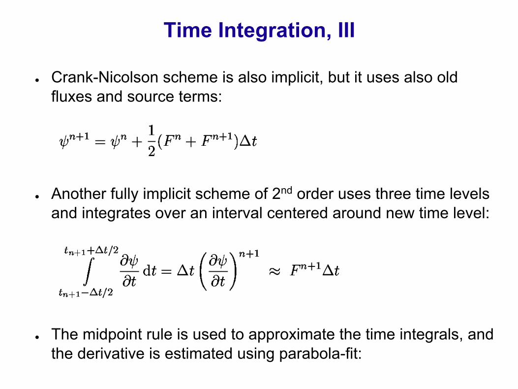
● Crank-Nicolson scheme is also implicit, but it uses also old fluxes and source terms:
● Another fully implicit scheme of 2nd order uses three time levels and integrates over an interval centered around new time level:
● The midpoint rule is used to approximate the time integrals, andthe derivative is estimated using parabola-fit:

Time Integration, IV
● This leads to the following form of the algebraic equation for one CV:

Grid Motion, I
● In the case of moving grids, the space-conservation law (SCL) has to be satisfied:
● In the case of constant density, the mass-conservation equation becomes:
● This shows that the SCL must be satisfied to ensure that the velocity field is divergence-free...

Grid Motion, II
● Discretized form of SCL, e.g. with the implicit three-time-levels scheme:
The volume change from one time step to the other can be expressed through volumes swept by cell faces:

Grid Motion, III
● The volume fluxes due to grid motion can also be expressed through swept volumes as:
This ensures that the SCLis satisfied automaticallyand the grid velocity neednot be explicitly computed...
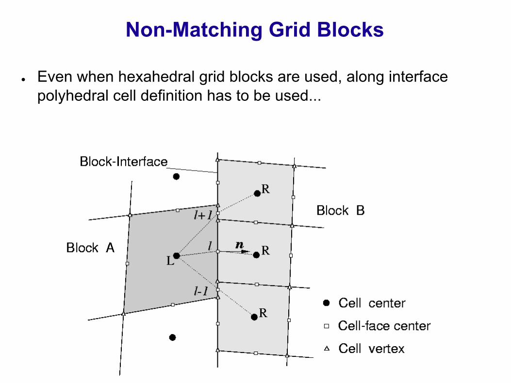
Non-Matching Grid Blocks
● Even when hexahedral grid blocks are used, along interface polyhedral cell definition has to be used...
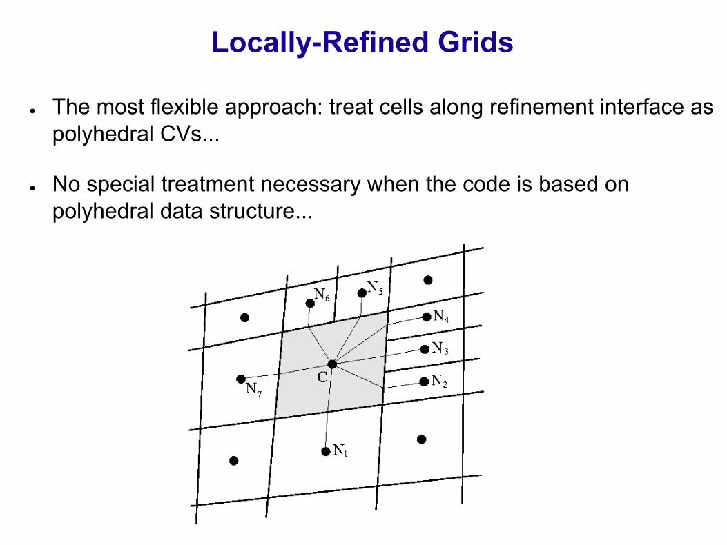
Locally-Refined Grids
● The most flexible approach: treat cells along refinement interface as polyhedral CVs...
● No special treatment necessary when the code is based on polyhedral data structure...

Sliding Grid Blocks
● Polyhedral CV data structure allows also simple treatment of sliding interfaces (same as non-matching grid blocks, but faces in the interface change with time in number and size...)
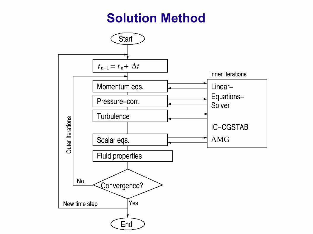
Solution Method
AMG

Free-Surface Flows
● Flows with free surfaces are often encountered in nature and engineering practice...
● Often only liquid flow is of interest...
● ... but sometimes the interaction of gas and liquid flow is essential.
● Main factors affecting free-surface flows are– Gravity (and other body forces)
– Surface tension

Interface-Tracking Method, I
● Flows with free surfaces can be computed by using either
– Interface-tracking methods and a moving, boundary-fitted grid (with free surface treated as a boundary between two fluids), or
– Interface-capturing methods, which compute the flow of both fluids on a fixed grid.
● Interface-tracking methods specify pressure at free surface using the dynamic boundary condition:

Interface-Tracking Method, II
● The position of the free surface is determined from the kinematic boundary condition:
● The prescribed pressure at free surface leads to non-zero mass fluxes (pressure correction is zero, velocity correction is not)...
● The free surface is then displaced to avoid fluid crossing the interface...
● Usually, only the flow of liquid is computed - in gas, constant pressure is assumed.
● Contact angle can be prescribed where the free surface is in contact with a solid wall.

Interface-Tracking Method, III
● The volume flux correction:
● Displacement of control and mesh points:
Interface-Tracking Method, IV
● The free surface is represented as a sharp interface...
● The grid must adapt to the shape and position of the free surface, and to solid walls...
● ... which can be difficult to automate, especially when walls have a complicated shape (e.g. some ship hulls...).
● The free surface should not overturn, gas enclosures or liquid drops are difficult to simulate -> re-griding may be necessary from time to time...
● This approach is usually used for shallow-water flows and flows with smooth free surface...

Interface-Capturing Method, I
● Interface-capturing method: gas and liquid are treated as an effective fluid with variable properties...
● The grid covers the whole solution domain and is only fitted to walls (which can move, so the grid moves with them)...
● The free surface lies in the transition region from one fluid to the other and is thus »captured«...
● Additional equations have to be solved for volume fractions of individual fluids (here assumed incompressible):

Interface-Capturing Method, II
● The free surface is not a sharp boundary between fluids - it is »smeared« over 1 – 2 cells...
● One can define the interface as the iso-surface c = 0.5
● For sharp interfaces, special discretization for convective terms in the equation for c is needed (to avoid excessive spreading)...
● A combination of upwind and downwind can be found, which fulfils these criteria...
● ...as well as the boundedness 0 <= c <= 1.
● Gas bubbles in liquid or liquid drops in gas can be simulated -interface sharpness can be increased by local grid refinement...
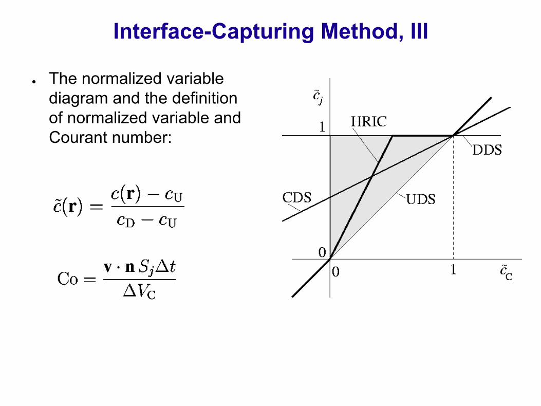
Interface-Capturing Method, III
● The normalized variable diagram and the definition of normalized variable and Courant number:

Interface-Capturing Method, IV
● The approximation of the face value depends on the free-surface shape:

Interface-Capturing Method, V
● The steps towards the final face value:
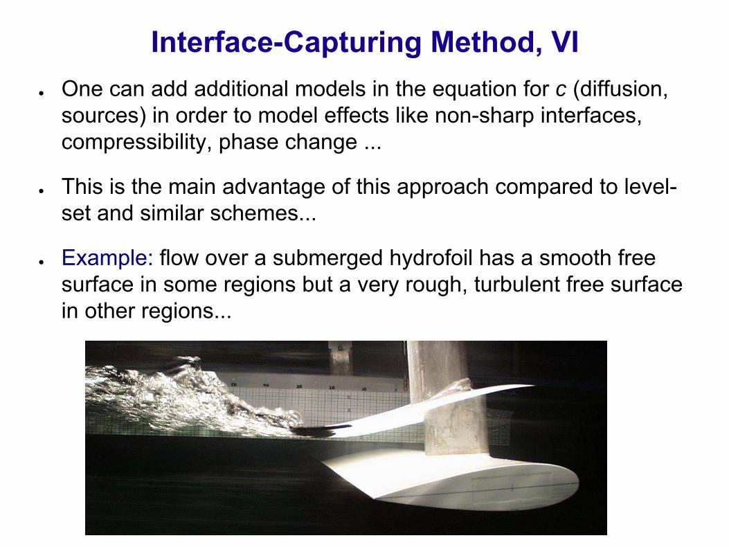
Interface-Capturing Method, VI● One can add additional models in the equation for c (diffusion,
sources) in order to model effects like non-sharp interfaces, compressibility, phase change ...
● This is the main advantage of this approach compared to level-set and similar schemes...
● Example: flow over a submerged hydrofoil has a smooth free surface in some regions but a very rough, turbulent free surfacein other regions...

Interface-Capturing Method, VII
● The effects of surface tension can be taken into account - as volume forces, which are active only in the interface region:
● The curvature of the interface can be obtained from the divergence of the unit vector normal to the interface c = 0.5; it is defined by the gradient of c:

Interface-Capturing Method, V
● The problem: parasitic currents can develop, if the fluid moves only slowly or not at all, and the surface tension plays an important role...
● The reason: pressure and surface tension forces must be in equilibrium - but the numerical approximations do not guarantee that...
● The solution approach: try to modify the surface-tension force so that the two terms can cancel exactly:

Validation, I
Critical flowover semi-cylinder onchannel bottom

Validation, II
Comparison of two simulation methods with experimental datafor the free-surface shape above the semi-cylinder

Validation, III
Simulation of breaking-dam flow

Examples of Application
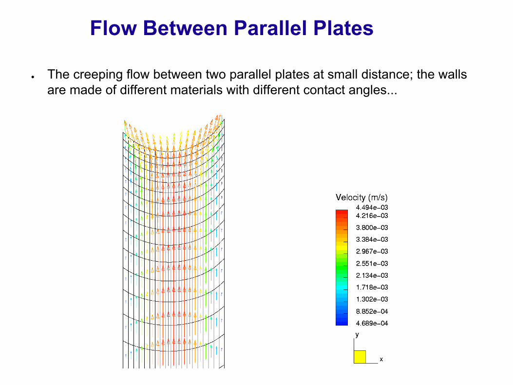
Flow Between Parallel Plates
● The creeping flow between two parallel plates at small distance; the walls are made of different materials with different contact angles...
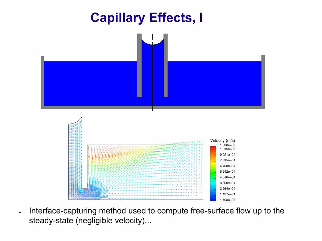
Capillary Effects, I
● Interface-capturing method used to compute free-surface flow up to the steady-state (negligible velocity)...
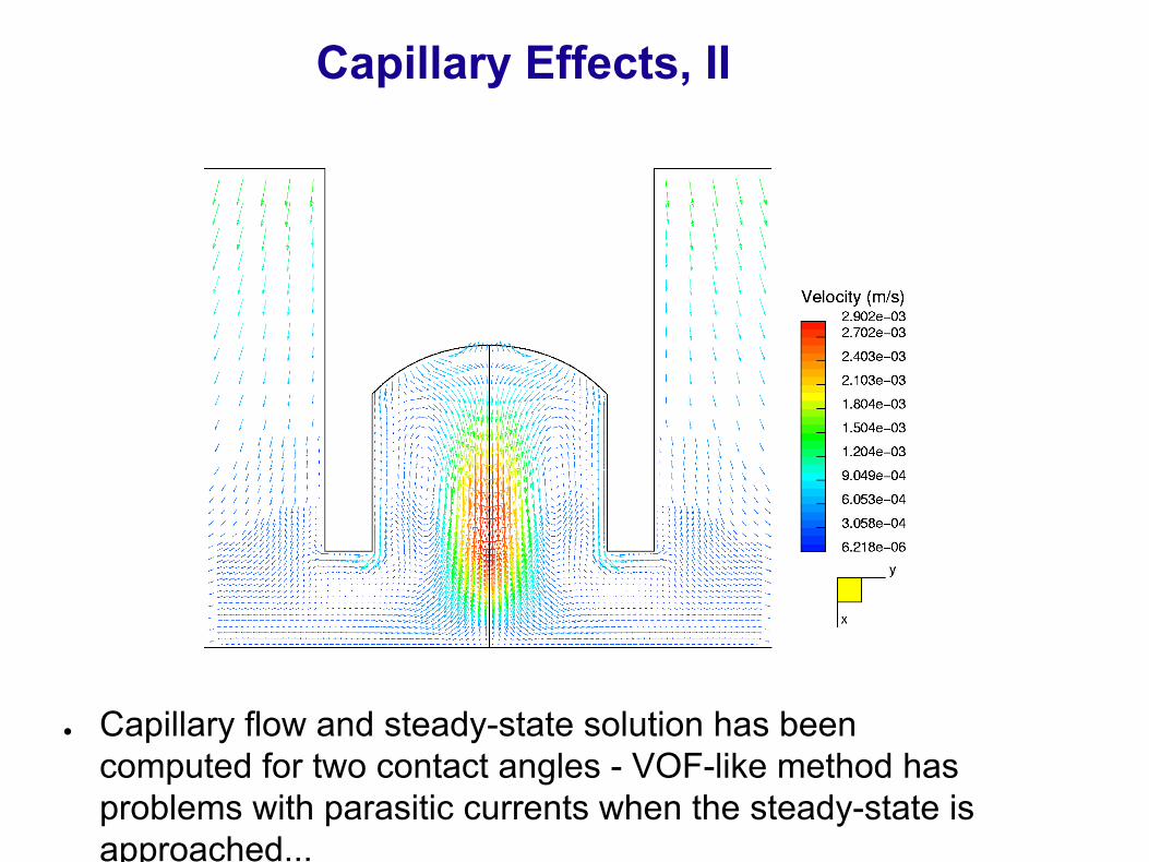
Capillary Effects, II
● Capillary flow and steady-state solution has been computed for two contact angles - VOF-like method has problems with parasitic currents when the steady-state is approached...
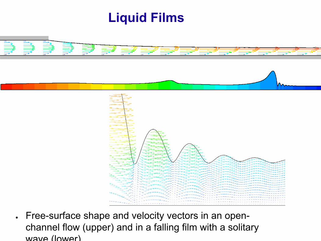
Liquid Films
● Free-surface shape and velocity vectors in an open-channel flow (upper) and in a falling film with a solitary wave (lower)

Rayleigh Jet Break-Up, I
● Rayleigh-break-up of a laminar jet for different amplitudes of excitation: (jet diameter D = 2,59 mm; flow velocity U = 2,126 m/s; amplitude of disturbance 1%; wave number k* = πD/L = 0,25; 0,43; 0,533; 0,683. From Albina, Muzaferija und Peric, 2000)
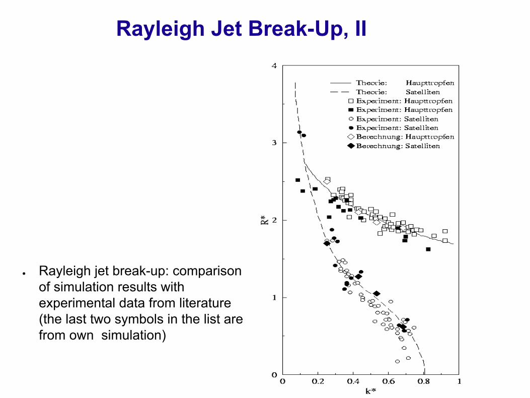
Rayleigh Jet Break-Up, II
● Rayleigh jet break-up: comparison of simulation results with experimental data from literature (the last two symbols in the list are from own simulation)
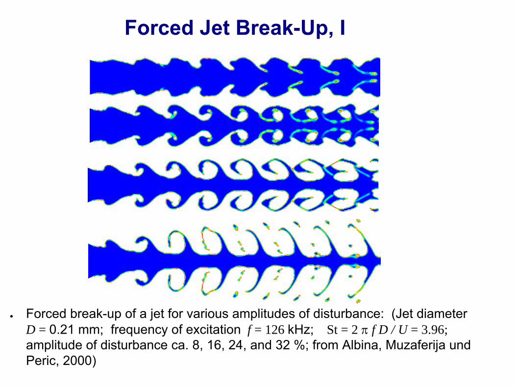
Forced Jet Break-Up, I
● Forced break-up of a jet for various amplitudes of disturbance: (Jet diameterD = 0.21 mm; frequency of excitation f = 126 kHz; St = 2 π f D / U = 3.96; amplitude of disturbance ca. 8, 16, 24, and 32 %; from Albina, Muzaferija und Peric, 2000)

Forced Jet Break-Up, II
● Experimental study of forced jet break-up showing similar phenomena as observed in the simulation (Bergakademie Freiberg, 1999/2000)
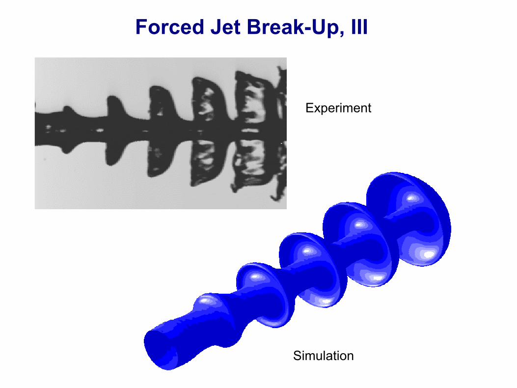
Forced Jet Break-Up, III
Experiment
Simulation

Droplet Impact on Wall, I
Comparison of visualization in experiment (left) and simulation (right) for a water droplet impact on waxed wall in the spreading phase (from PhD thesis of S. Sikalo, TU Darmstadt, 2003)

Droplet Impact on Wall, II
Comparison of water droplet spreading diameter on waxed wall as a function of time observed in experiment and in simulation (from PhD thesis of S. Sikalo, TU Darmstadt, 2003)

Detail...
Roll-Coater
● The whole roll-coater has been simulated, starting from a flat surface in the tank...

Nozzle Flows, I
Inlet pipe diameter 2,4 mmNozzle diameter 4,8 mmInlet water velocity ca. 11 m/s
InletInlet
Exit

Nozzle Flows, II
Air core inside nozzle: stable, helical...
Air
LiquidSimulation
Experiment
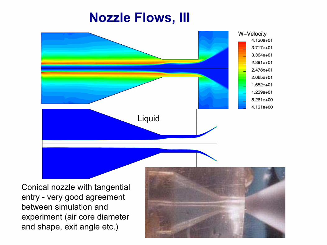
Nozzle Flows, III
Conical nozzle with tangentialentry - very good agreement between simulation and experiment (air core diameterand shape, exit angle etc.)
Liquid
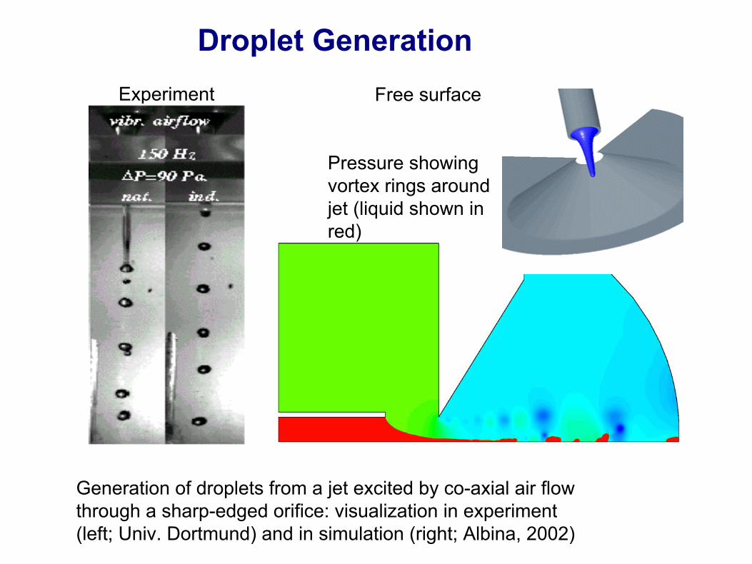
Droplet GenerationExperiment Free surface
Pressure showingvortex rings aroundjet (liquid shown inred)
Generation of droplets from a jet excited by co-axial air flowthrough a sharp-edged orifice: visualization in experiment (left; Univ. Dortmund) and in simulation (right; Albina, 2002)
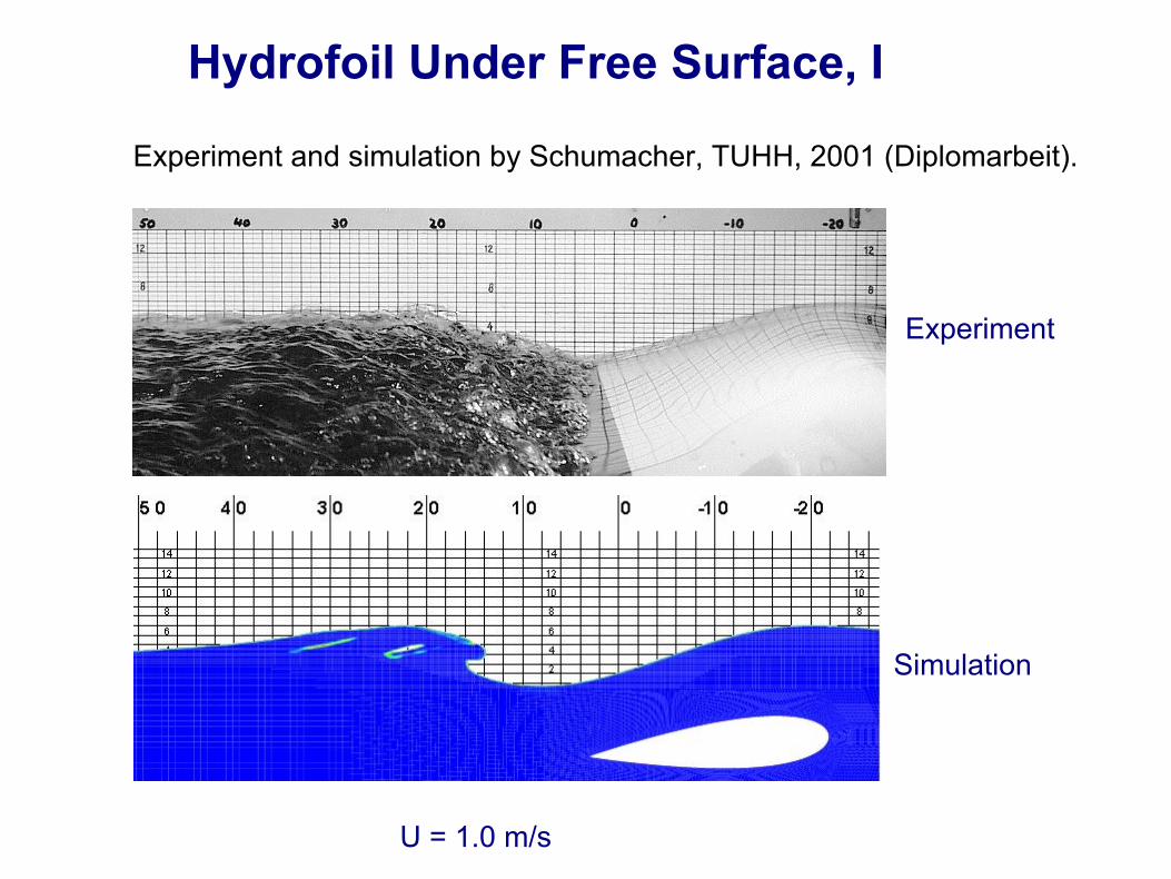
Hydrofoil Under Free Surface, I
Experiment and simulation by Schumacher, TUHH, 2001 (Diplomarbeit).
Experiment
Simulation
U = 1.0 m/s

Hydrofoil Under Free Surface, II
Experiment
Simulation
U = 1.2 m/s

Hydrofoil Under Free Surface, III
The existence of wave breaking and the wave length/height well predicted...
Experiment
Simulation
U = 1.4 m/s

Cars on Flooded Deck, I
Model experimentand simulationperformed at TUHH(2000)
Experiment
Simulation

Cars on Flooded Deck, II
The shape of freesurface deformation as a function of waterdepth and car shapequalitatively wellpredicted...
Experiment
Simulation

Flow Around Ship Model with Blunt Bow, I
Breakingwave atstern
Experiment, SRIExperiment, SRI
Simulation (Azcueta, PhD Thesis, TUHH, 2000)

Flow Around Ship Model with Blunt Bow, III
Average water level in symmetry plane and along hull, and average velocities in symmetry plane in water and air

Flow Around Ship Model with Blunt Bow, IV
Symmetry Hull Symmetry
Comparison of wave profile along hull computed at TUHH withexperimental data obtained at Ship Research Institute, Tokyo

Flow Around Surface-Piercing Propellers
Pressure distribution on a surface-piercing propeller (left) and a comparison of simulation results with cavitation tank data (courtesy of Rolla SP Propellers SA)

Ship in Shallow Water over Mud, I
Ship in a channel, mud on bottom (density 5% higher than in water, viscosity 400 times higher); motion from left to right...
Air
Water
Mud
Ship motion
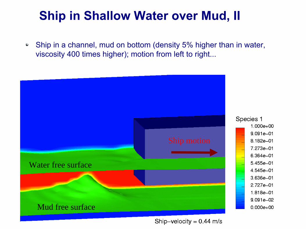
Ship in Shallow Water over Mud, II
Ship in a channel, mud on bottom (density 5% higher than in water, viscosity 400 times higher); motion from left to right...
Water free surface
Mud free surface
Ship motion

Sloshing in a Rectangular Tank, I
3D flow simulation, sway motion: free-surface deformation...

Sloshing in a Rectangular Tank, II
3D flow simulation, sway motion: free-surface deformation...

Sloshing in a Rectangular Tank, III
Period 1.85 s
(resonance)
Period 2.25 s
(off-resonance)
● Pressure variation at location P1 over 10 periods of roll motion: comparison with experimental data.

Validation Test Case: Comparison With Experiment, IISloshing in a Rectangular Tank, IV
Period 1.85 s
(resonance)
Period 2.25 s
(off-resonance)
● Pressure variation at location P3 over 10 periods of roll motion: comparison with experimental data.

Optimization of Hull FormHull Optimization
● Voith should deliver a propeller but found that small changes to the hull form could improve the efficiency by 30% - much more than optimization of the propeller! Experiment at SVA Potsdam verified CFD results...
Optimized designOriginal design
Courtesy of Voith Turbo Marine GmbH & Co. KG

Hull-Propeller InteractionOptimization of Hull Form
● Simulations are performed with rotating propellers, all relevant hull appendages, and deforming free surface, taking into account all non-linear interactions...
Pressure distribution on hull, propeller blades and guard plate, and free-surface deformation, viewed from below (left) and above (right)
Courtesy of Voith Turbo Marine GmbH & Co. KG