computation of 3d flows with violent free surface...

Computation of 3D Flows with Violent Free Surface MotionChi Yang1 and Rainald Lohner

School of Computational Sciences, George Mason UniversityFairfax, Virginia, U.S.A.

ABSTRACT

A robust Volume of Fluid (VOF) technique is presented togetherwith an incompressible Euler/Navier Stokes solver operating onadaptive, unstructured grids to simulate the interactions of ex-treme waves and three-dimensional structures. The incompress-ible Euler/Navier Stokes equations are solved using projectionschemes and a finite element method. The classic breaking damproblem is first used to validate the three-dimensional computercode developed based on the method described above. The com-puter code is then used to simulate the sloshing of a partially filledtwo-dimensional tank due to sway excitation. The resulting waveheights and pressure forces for various excitation frequencies andamplitudes are compared with experimental data and those pre-dicted by the SPH method. The numerical simulation of the slosh-ing of a partially filled three-dimensional tank is carried out andcompared with its counterpart of a two-dimensional tank. Thecomputational results demonstrate that the present CFD methodis capable of simulating the violent resonant free surface flowswith strong nonlinear behavior in a partially filled tank, which isof great importance to the offshore and shipping industry.

KEY WORDS: Finite element method, VOF method, violent freesurface flows, sloshing, nonlinear hydrodynamics, wave loading.

INTRODUCTION

In rough seas, ships or offshore structures may experience highlynonlinear phenomena such as slamming and green water on deck.Impact loads due to slamming and green water shipping are asso-ciated with the three dimensional flows with a violent free surface.A ship carrying liquid cargo in partially filled tanks in waves mayexperience violent sloshing even in low sea state. When the forc-ing frequencies are in the vicinity of the lowest natural frequencyfor the fluid motion inside a smooth tank, a violent free surface

1Cheung Kong Scholar, Shanghai Jiao Tong University.

wave may be observed even if the tank oscilates with a small am-plitude. The resulting impact loads are also due to the violent freesurface motion. These impact loads are of considerable concernand there is a great need for the calculation method to simulatethe three dimensional flows with a violent free surface motion.

The computation of highly nonlinear free surface flows is dif-ficult because neither the shape nor the position of the interfacebetween air and water is known a priori; on the contrary, it of-ten involves unsteady fragmentation and merging process. Thereare basically two approaches to compute flows with free surface:interface-tracking and interface-capturing methods. The formercompute the liquid flow only, using a numerical grid that adaptsitself to the shape and position of the free surface. The free sur-face is represented and tracked explicitly either by marking it withspecial marker points, or by attaching it to a mesh surface. Var-ious surface fitting methods for attaching the interface to a meshsurface were developed during the past decades using the finite el-ement method. In the interface tracking methods, the free surfaceis treated as a boundary of the computational domain, where thekinematic and dynamic boundary conditions are applied. Thesemethods can not be used if the interface topology changes signif-icantly (e.g. overturning or breaking waves).

On the other hand, interface-capturing methods consider bothfluids as a single effective fluid with variable properties; the inter-face is captured as a region of sudden change in fluid properties.Either massless particles or an indicator function marks gas orfluid on either side of the interface. Among various interface-capturing methods, volume-of-fluid (VOF) methods and level-set(LS) methods are more economical than marker particles, as onlyone value (the volume fraction for VOF or the level-set functionfor LS) needs to be assigned to each mesh cell. Another ben-efit of using volume fractions or level-set functions is that onlya scalar convection equation needs to be solved to propagate thevolume fractions or level-set functions through the computationaldomain. The interface-capturing methods based on the Eulerianapproach require no geometry manipulations after the mesh isgenerated and can be applied to interfaces of a complex topology

Paper No. 2005-JSC-284 Yang Page number: 1

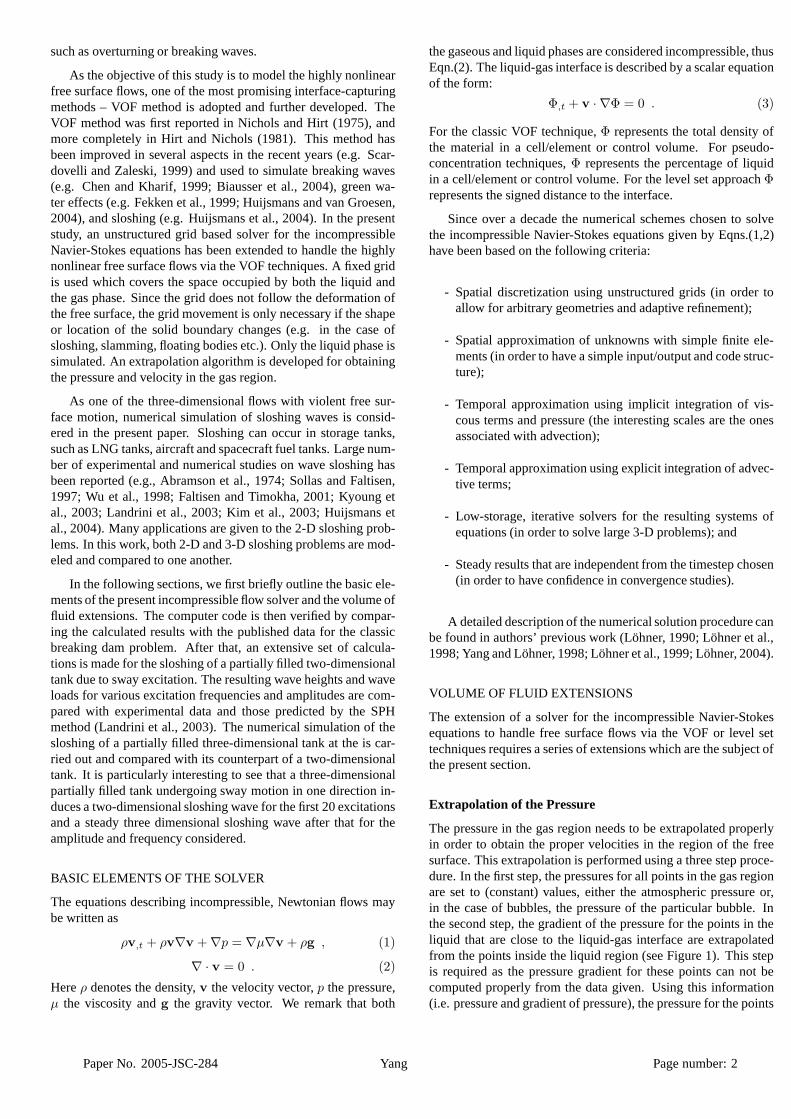
such as overturning or breaking waves.

As the objective of this study is to model the highly nonlinearfree surface flows, one of the most promising interface-capturingmethods – VOF method is adopted and further developed. TheVOF method was first reported in Nichols and Hirt (1975), andmore completely in Hirt and Nichols (1981). This method hasbeen improved in several aspects in the recent years (e.g. Scar-dovelli and Zaleski, 1999) and used to simulate breaking waves(e.g. Chen and Kharif, 1999; Biausser et al., 2004), green wa-ter effects (e.g. Fekken et al., 1999; Huijsmans and van Groesen,2004), and sloshing (e.g. Huijsmans et al., 2004). In the presentstudy, an unstructured grid based solver for the incompressibleNavier-Stokes equations has been extended to handle the highlynonlinear free surface flows via the VOF techniques. A fixed gridis used which covers the space occupied by both the liquid andthe gas phase. Since the grid does not follow the deformation ofthe free surface, the grid movement is only necessary if the shapeor location of the solid boundary changes (e.g. in the case ofsloshing, slamming, floating bodies etc.). Only the liquid phase issimulated. An extrapolation algorithm is developed for obtainingthe pressure and velocity in the gas region.

As one of the three-dimensional flows with violent free sur-face motion, numerical simulation of sloshing waves is consid-ered in the present paper. Sloshing can occur in storage tanks,such as LNG tanks, aircraft and spacecraft fuel tanks. Large num-ber of experimental and numerical studies on wave sloshing hasbeen reported (e.g., Abramson et al., 1974; Sollas and Faltisen,1997; Wu et al., 1998; Faltisen and Timokha, 2001; Kyoung etal., 2003; Landrini et al., 2003; Kim et al., 2003; Huijsmans etal., 2004). Many applications are given to the 2-D sloshing prob-lems. In this work, both 2-D and 3-D sloshing problems are mod-eled and compared to one another.

In the following sections, we first briefly outline the basic ele-ments of the present incompressible flow solver and the volume offluid extensions. The computer code is then verified by compar-ing the calculated results with the published data for the classicbreaking dam problem. After that, an extensive set of calcula-tions is made for the sloshing of a partially filled two-dimensionaltank due to sway excitation. The resulting wave heights and waveloads for various excitation frequencies and amplitudes are com-pared with experimental data and those predicted by the SPHmethod (Landrini et al., 2003). The numerical simulation of thesloshing of a partially filled three-dimensional tank at the is car-ried out and compared with its counterpart of a two-dimensionaltank. It is particularly interesting to see that a three-dimensionalpartially filled tank undergoing sway motion in one direction in-duces a two-dimensional sloshing wave for the first 20 excitationsand a steady three dimensional sloshing wave after that for theamplitude and frequency considered.

BASIC ELEMENTS OF THE SOLVER

The equations describing incompressible, Newtonian flows maybe written as

ρv,t + ρv∇v + ∇p = ∇µ∇v + ρg , (1)

∇ · v = 0 . (2)

Here ρ denotes the density, v the velocity vector, p the pressure,µ the viscosity and g the gravity vector. We remark that both

the gaseous and liquid phases are considered incompressible, thusEqn.(2). The liquid-gas interface is described by a scalar equationof the form:

Φ,t + v · ∇Φ = 0 . (3)

For the classic VOF technique, Φ represents the total density ofthe material in a cell/element or control volume. For pseudo-concentration techniques, Φ represents the percentage of liquidin a cell/element or control volume. For the level set approach Φrepresents the signed distance to the interface.

Since over a decade the numerical schemes chosen to solvethe incompressible Navier-Stokes equations given by Eqns.(1,2)have been based on the following criteria:

- Spatial discretization using unstructured grids (in order toallow for arbitrary geometries and adaptive refinement);

- Spatial approximation of unknowns with simple finite ele-ments (in order to have a simple input/output and code struc-ture);

- Temporal approximation using implicit integration of vis-cous terms and pressure (the interesting scales are the onesassociated with advection);

- Temporal approximation using explicit integration of advec-tive terms;

- Low-storage, iterative solvers for the resulting systems ofequations (in order to solve large 3-D problems); and

- Steady results that are independent from the timestep chosen(in order to have confidence in convergence studies).

A detailed description of the numerical solution procedure canbe found in authors’ previous work (Lohner, 1990; Lohner et al.,1998; Yang and Lohner, 1998; Lohner et al., 1999; Lohner, 2004).

VOLUME OF FLUID EXTENSIONS

The extension of a solver for the incompressible Navier-Stokesequations to handle free surface flows via the VOF or level settechniques requires a series of extensions which are the subject ofthe present section.

Extrapolation of the Pressure

The pressure in the gas region needs to be extrapolated properlyin order to obtain the proper velocities in the region of the freesurface. This extrapolation is performed using a three step proce-dure. In the first step, the pressures for all points in the gas regionare set to (constant) values, either the atmospheric pressure or,in the case of bubbles, the pressure of the particular bubble. Inthe second step, the gradient of the pressure for the points in theliquid that are close to the liquid-gas interface are extrapolatedfrom the points inside the liquid region (see Figure 1). This stepis required as the pressure gradient for these points can not becomputed properly from the data given. Using this information(i.e. pressure and gradient of pressure), the pressure for the points


in the gas that are close to the liquid-gas interface are computed.

p

p

p=pgp=pg

p=pg

p

p

Liquid

Interface

Gas

p

pp

p

p

p

Figure 1: Extrapolation of the Pressure

Extrapolation of the Velocity

The velocity in the gas region needs to be extrapolated properly inorder to propagate accurately the free surface. This extrapolationis started by initializing all velocities in the gas region to v =0. Then, for each subsequent layer of points in the gas regionwhere velocities have not been extrapolated (unknown values),an average of the velocities of the surrounding points with knownvalues is taken (see Figure 2).

Interface

v

v

v

Layer 1

Layer 2

Gas

Liquid

v

Figure 2: Extrapolation of the Velocity

Imposition of Constant Mass

Experience indicates that the amount of liquid mass (as measuredby the region where the VOF indicator is larger than a cut-offvalue) does not remain constant for typical runs. The reasons forthis loss or gain of mass are manifold: loss of steepeness in theinterface region, inexact divergence of the velocity field, bound-ary velocities, etc. This lack of exact conservation of liquid masshas been reported repeatedly in the literature. The recourse takenhere is the classic one: add/remove mass in the interface regionin order to obtain an exact conservation of mass. At the end ofevery timestep, the total amount of fluid mass is compared to theexpected value. The expected value is determined from the massat the previous timestep, plus the mass-flux across all boundariesduring the timestep. The differences in expected and actual massare typically very small, so that quick convergence is achieved bysimply adding and removing mass appropriately. The amount ofmass taken/added is made proportional to the absolute value of

the normal velocity of the interface:

vn =

∣

∣

∣

∣

v ·∇Φ

|∇Φ|

∣

∣

∣

∣

. (4)

In this way the regions with no movement of the interface remainunaffected by the changes made to the interface in order to im-pose strict conservation of mass.

Deactivation of Air Region

Given that the air region is not treated/updated, any CPU spenton it may be considered wasted. Most of the work is spent inloops over the edges (upwind solvers, limiters, gradients, etc.).Given that edges have to be grouped in order to avoid memorycontention/ allow vectorization when forming right-hand sides(Lohner, 1993, Lohner, 1998), this opens a natural way of avoid-ing unnecessary work: form relatively small edge-groups that stillallow for efficient vectorization, and deactivate groups instead ofindividual edges (Lohner, 2001). In this way, the basic loopsover edges do not require any changes. The if-test whether anedge group is active or deactive occurs outside the inner loopsover edges, leaving them unaffected. On scalar processors, edges-groups as small as negrp=8 are used. Furthermore, if points andedges are grouped together in such a way that proximity in mem-ory mirrors spatial proximity, most of the edges in air will notincur any CPU penalty.

NUMERICAL RESULTS

In the following examples, the fluid is assumed to be a laminarNewtonian fluid with reference viscosity µ = 0.01. The freeslip condition is imposed on the solid boundaries. The numericalforce is calculated by integrating the pressure force.

Breaking Dam Problem

This is a classic test case for free surface flows. The problemdefinition is shown in Figure 4a.

14.0

7.0

3.5

10.0ρ=0.9982µ=0.01 g=(0,−1,0)

Figure 4a: Breaking Dam: Problem Definition

This case was run on a coarse mesh with nelem=16,562 ele-ments, a fine mesh with nelem=135,869 and an adaptively re-fined mesh (where the coarse mesh was the base mesh) with ap-proximately nelem=30,000 elements. The refinement indicatorfor the latter was the free surface, and the mesh was adapted ev-ery 5 time steps. Figure 4b shows the discretization for the coarse


mesh. The results obtained for the horizontal location of the freesurface along the bottom wall are compared to the experimentalvalues of Martin and Moyse (1952), as well as the numerical re-sults obtained by Hansbo (1992), Kolke (2005), Walhorn (2002)in Figure 4c. The dimensionless time and displacement are givenby τ = t

√

2g/a and δ = x/a. As one can see, the agreementis very good, even for the coarse mesh. The difference betweenthe adaptively refined mesh and the fine mesh was almost indis-tinguishable, and therefore only the resuls for the fine mesh areshown in the graph. Figure 4d shows the flow field and free sur-face at a given time t = 3.

Figure 4b: Breaking Dam: Discretization forthe Coarse Mesh

1.0

1.5

2.0

2.5

3.0

3.5

4.0

0.0 0.5 1.0 1.5 2.0 2.5 3.0

dim

ensi

onle

ss d

ispl

acem

ent

dimensionless time

Martin/MoyceHansbo

WalhornSauer

KoelkeFEFLO CoarFEFLO Fine

Figure 4c: Breaking Dam: Horizontal Displacement

Figure 4d: Breaking Dam: Flowfield at t=3.

Sloshing of a 2D Tank due to Sway Excitation

In the previous section, we have already verified the accuracy ofour numerical model for studing wave breaking. In this section,we shall apply our numerical model to study the sloshing of apartially filled 2D tank. The main tank dimensions are L = H =1m , with tank width b = 0.1m. The problem definition is shownin Figure 5a. This case is run on a mesh with nelem=54,124

elements.

Y

L=1m

H=1m

A1

50mmA

h=0.35m

X

Figure 5a: 2D Tank: Problem Definition

Experimental data for the above tank with a filling level h/L =0.35 have been provided by Olsen (1970), and reported in Fal-tisen (1974) and Olsen and Johnsen (1975), where the tank wasundergoing a sway motion, i.e., the tank oscillates horizontallywith law Asin(2πt/T ). A wave gage was placed 0.05m fromthe right wall and the maximum wave elevation relative to a tank-fixed coordinate system was recorded. In the numerical simula-tions reported by Landrini et al. (2003) using the SPH method,the forced oscillation amplitude increases smoothly in time andreaches its steady regime value in 10T. The simulation continuesfor another 30T, and the maximum wave elevation is recorded inlast 10 periods of oscillation.

We followed the same procedure as Landrini et al. (2003)in our numerical simulation for 32 cases, which correspond to2 amplitudes (A = 0.025, 0.05) and 16 periods, ranging fromT = 1 − 1.8 seconds or T/T1 = 0.787 − 1.42, where T1 =1.27 seconds. When h/L = 0.35 the primary resonances of thefirst and the third modes occur at T/T1 = 1 and T/T1 = 0.55,respectively. The secondary resonance of the second mode is atT/T1 = 1.28 (see Landrini et al. 2003).

The present VOF results for the time history of the lateralforce Fx when T = 1.2, 1.3 and A = 0.025, 0.05 are shownin Figure 5b. The corresponding time history of the wave eleva-tion at the wave probe A1 (see Figure 5a) are shown in Figure 5c.Some free surface snapshots are shown in Figure 5d.

The present VOF results for maximum wave elevation ζ at thewave probe A1 (see Figure 5a) are compared with the experimen-tal data and SPH results (Landrini et al. 2003) in Figures 5e for


A/L = 0.025, 0.05. The predicted lateral absolute values of max-imum forces are compared with the experimental data and SPHresults (Landrini et al. 2003) in Figure 5f for A/L = 0.05 (Thereis no force data available for A/L = 0.025). Figure 5g showsthe comparison of predicted lateral absolute values of maximumforces for A/L = 0.025, 0.05. It can be seen from Figures 5e-f that both maximum wave height and lateral absolute values ofmaximum forces predicted by present VOF method agrees fairlywell with the experimental data and SPH results except there is asmall phase shift among three results.

-150

-100

-50

0

50

100

150

0 5 10 15 20 25 30 35 40

F x 1

03 /ρ g

L2 b

t/T

VOF, T=1.2, A/L=0.025

-150

-100

-50

0

50

100

150

0 5 10 15 20 25 30 35 40

F x 1

03 /ρ g

L2 b

t/T

VOF, T=1.2, A/L=0.05

-150

-100

-50

0

50

100

150

0 5 10 15 20 25 30 35 40

F x 1

03 /ρ g

L2 b

t/T

VOF, T=1.3, A/L=0.025

-150

-100

-50

0

50

100

150

0 5 10 15 20 25 30 35 40

F x 1

03 /ρ g

L2 b

t/T

VOF, T=1.3, A/L=0.05

Figure 5b: 2D Tank: Time History of Lateral Force Fx

-0.6

-0.4

-0.2

0

0.2

0.4

0.6

0 5 10 15 20 25 30 35 40

wav

e el

evat

ion

(ζ /L

)

t/T

VOF, T=1.2, A/L=0.025

-0.6

-0.4

-0.2

0

0.2

0.4

0.6

0 5 10 15 20 25 30 35 40

wav

e el

evat

ion

(ζ /L

)

t/T

VOF, T=1.2, A/L=0.05

-0.6

-0.4

-0.2

0

0.2

0.4

0.6

0 5 10 15 20 25 30 35 40

wav

e el

evat

ion

(ζ /L

)

t/T

VOF, T=1.3, A/L=0.025

-0.6

-0.4

-0.2

0

0.2

0.4

0.6

0 5 10 15 20 25 30 35 40

wav

e el

evat

ion

(ζ /L

)

t/T

VOF, T=1.3, A/L=0.05

Figure 5c: 2D Tank: Time History of Wave Elevationat the Wave Probe A1

Figures 5b and 5c are typical time history plots. It should benoted from these figures that even after a long simulation time (40periods), steady state results are not generally obtained. This isdue to very small damping in the system. Landrini et al. (2003)noted the same behavior in their numerical simulations. As a re-sult, the predicted maximum wave elevation and the lateral abso-lute values of maximum forces ploted in Figure 5e are averagemaximum values for the last few periods for the cases when thesteady state is not reached.


Figure 5d: 2D Tank: Snapshots of Free Surface WaveElevation for T = 1.3 and A/L = 0.05

0

0.1

0.2

0.3

0.4

0.5

0.6

0.7

0.7 0.8 0.9 1 1.1 1.2 1.3 1.4 1.5

wav

e he

ight

(ζ

/L)

T/T1

VOF, A/L=0.025Exp, A/L=0.025SPH, A/L=0.025

0

0.1

0.2

0.3

0.4

0.5

0.6

0.7

0.7 0.8 0.9 1 1.1 1.2 1.3 1.4 1.5

wav

e he

ight

(ζ

/L)

T/T1


Figure 5e: 2D Tank: Maximum Wave Heightat the Wave Probe A1

0

20

40

60

80

100

120

140

160

180

0.7 0.8 0.9 1 1.1 1.2 1.3 1.4 1.5

F x 1

03 /ρ g

L2 b

T/T1


Figure 5f: 2D Tank: Maximum Absolute Values ofLateral Force Fx for A/L = 0.05

0

20

40

60

80

100

120

140

160

180

0.7 0.8 0.9 1 1.1 1.2 1.3 1.4 1.5

F x 1

03 /ρ g

L2 b

T/T1

VOF, A/L=0.050VOF, A/L=0.025

Figure 5g: 2D Tank: Predicted Maximum Absolute Valuesof Lateral Force Fx for A/L = 0.025, 0.05

Sloshing of a 3D Tank due to Sway Excitation

In order to study the three dimensional effects, the sloshing of apartially filled 3D tank is then considered. The main tank dimen-sions are L = H = 1m , with tank width b = 1m. The problemdefinition is shown in Figure 6a. The 3D tank has the same filling


level h/L = 0.35 as the 2D tank. The 3D tank case is run on amesh with nelem=561,808 elements, and the 2D tank is run ona mesh with nelem=54,124 elements.

L=1m

H=1mX

h=0.35m

Y

Ab=1m

Z

Figure 6a: 3D Tank: Problem Definition

The numerical simulations are carried out for both 3D and 2Dtanks, where both tanks are undergoing the prescribed sway mo-tion, i.e., the tanks oscillate horizontally with law Asin(2πt/T ).The simulations were carried out for A = 0.025 and T = 1.27 orT/T1 = 1. The forced oscillation amplitude increases smoothlyin time and reaches its steady regime value in 10T. The simulationcontinues for another 70T.

In order to show the 3D effects, the forces are nondimension-alized with ρgL2b for both 2D and 3D tanks. Figures 6b,c showthe time history of the force Fx (horizontal force in the same di-rection as the tank moving direction) for both 2D and 3D tanks.Figure 6d shows the time history of the force Fz (horizontal forceperpendicular to the tank moving direction) for 3D tank. It is veryinteresting to observe from Figures 6c,d that there are almost no3D effects for the first 25 oscillating periods. The 3D modes startto appear after 25T, and fully build up at about 40T. The 3D flowpattern then remains steady and periodic for the rest of the simu-lation, which is about 40 more oscillating periods.

Figures 7a-c show a sequence of snapshots of the free surfacewave elevation for the 3D tank. For the first set of snapshots (seeFigure 7a), the flow is still two-dimensional. The 3D flow startsto build up in the second set of snapshots (see Figure 7b). Theflow remains periodic three-dimensional for the last 40 periods.Figure 7c show the typical snapshots of the free surface for thelast 40 periods. The 3D effects are clearly shown in these plots.Figure 8 show a sequence of snapshots of the free surface waveelevation for the 2D tank at the same time instance as those shownin Figure 7a. The flow remains periodic two-dimensional for therest of the simulation.

CONCLUSIONS

A robust Volume of Fluid (VOF) technique has been devel-oped and coupled with an incompressible Euler/Navier Stokessolver operating on adaptive, unstructured grids to simulate theinteractions of extreme waves and three-dimensional structures.In the present approach, only the liquid phase needs to be simu-lated. An effective extrapolation technique has been developed toobtain the pressure and velocity in the gas region.

In this study, the classic breaking dam problem has been usedto verify the computer code. The results obtained for the horizon-tal location of the free surface along the bottom wall are comparedto the experimental values and other numerical predictions. Theagreement is very good, even for the coarse mesh.

An extensive set of calculations is then performed for thesloshing of a partially filled 2D tank due to sway excitation. Theresulting wave heights and wave loads for various excitation fre-quencies and amplitudes are compared with experimental dataand those predicted by the SPH method (Landrini et al., 2003).The agreement is fairly well. Finally, the numerical simulation ofthe sloshing of a partially filled 3D tank is carried out and com-pared with its counterpart of a 2D tank. It is particularly interest-ing to see that a 3D partially filled tank undergoing sway motionin one direction induces a two-dimensional sloshing wave for thefirst 20 excitations and a steady three dimensional sloshing waveafter that.

Computational results have demonstrated that the presentCFD method is capable of simulating the 3D flows with a violentfree surface motion, which is of great importance to the offshoreand shipping industry.

ACKNOWLEDGMENTS

The authors wish to thank Mr. Andrea Colagrossi of the INSEANfor providing both experimental data and numerical results for thesloshing of a 2D tank.

REFERENCES

Abramson, H.N., 1996, ”The dynamic Behaviour of Liquid inMoving Containers,” Reports SP 106 of NASA.

Alessandrini, B. and Delhommeau, G., 1996, ”A MultigridVelocity- Pressure-Free Surface Elevation Fully CoupledSolver for Calculation of Turbulent Incompressible FlowAround a Hull,” Proc. 21st Symp. on Naval Hydrodynamics,Trondheim, Norway, June.

Bell, J.B., Colella, P. and Glaz, H., 1989, ”A Second-Order Pro-jection Method for the Navier-Stokes Equations,” J. Comp.Phys. 85, 257-283.

Bell, J.B. and Marcus, D.L., 1992, ”A Second-Order ProjectionMethod for Variable-Density Flows,” J. Comp. Phys. 101, 2.

Biausser, B., Fraunie, P., Grilli, S. and Marcer R., 2004, ”Numer-ical analysis of the internal kinematics and dynamics of three-dimensional breaking waves on slopes,” International Journalof Offshore and Polar Engineering, Vol. 14, No. 4.

Chen, G., Kharif, C., 1999, ”Two-Dimensional Navier-StokesSimulation of Breaking Waves,” Physics of Fluids, 11(1), 121-133.


-150

-100

-50

0

50

100

150

0 10 20 30 40 50 60 70 80

F x 1

03 /ρ g

L2 b

t/T

VOF, A/L=0.025, 2D Tank

Figure 6b: 3D Tank: Time History of Force Fx for a 2D Tank at A/L = 0.025, T/T1 = 1)

-150

-100

-50

0

50

100

150

0 10 20 30 40 50 60 70 80

F x 1

03 /ρ g

L2 b

t/T


Figure 6c: 3D Tank: Time History of Force Fx for a 3D Tank at A/L = 0.025, T/T1 = 1)

-150

-100

-50

0

50

100

150

0 10 20 30 40 50 60 70 80

F z 1

03 /ρ g

L2 b

t/T


Figure 6d: 3D Tank: Time History of Force Fz for a 3D Tank at A/L = 0.025, T/T1 = 1)


Figure 7a: Snap Shots of the Free Surface Wave Elevation for 3D Tank


Figure 7b: Snap Shots of the Free Surface Wave Elevation for 3D Tank


Figure 7c: Snap Shots of the Free Surface Wave Elevation for 3D Tank


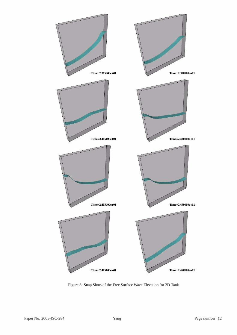
Figure 8: Snap Shots of the Free Surface Wave Elevation for 2D Tank


Codina, R., 2001, ”Pressure Stability in Fractional Step FiniteElement Methods for Incompressible Flows,” J. Comp. Phys.170, 112-140.

Faltisen, O.M., 1974, ”A Nonlinear Theory of Sloshing in Rect-angular Tanks,”, Journal of Ship Research, 18/4, pp. 224-241.

Faltisen, O.M. and Timokha A.N., 2001, ”Adaptive MultimodalApproach to Nonlinear Sloshing in a Rectangular Tank,” Jour-nal of Fluid Mechanics, Vol. 432, pp. 167-200.

Fekken, G., Veldman, A.E.P. and Buchner, B., 1999, ”Simulationof Green Water Loading Using the Navier-Stokes Equations,”Proceedings of the 7th International Conference on Numeri-cal Ship Hydrodynamics, Nantes, France.

Hansbo, P., 1992, ”The Characteristic Streamline DiffusionMethod for the Time-Dependent Incompressible Navier-Stokes Equations,” Comp. Meth. Appl. Mech. Eng. 99, 171-186.

Hirt, C.W. and Nichols, B.D., 1981, ”Volume of Fluid (VOF)Method for the Dynamics of Free Boundaries,” Journal ofComputational Physics 39, 201.

Huijsmans, R.H.M. and van Grosen, E., 2004, ”Coupling FreakWave Effects with Green Water Simulations,” Proceeding ofthe 14th ISOPE, Toulon, France, May 23-28.

Kallinderis, Y. and Chen, A., 1996, ”An Incompressible 3-DNavier-Stokes Method with Adaptive Hybrid Grids,” AIAA-96-0293.

Karbon, K.J. and Kumarasamy, S., 2001, ”Computational Aeroa-coustics in Automotive Design, Computational Fluid andSolid Mechanics,” Proc. First MIT Conference on Compu-tational Fluid and Solid Mechanics, 871-875, Boston.

Karbon, K.J. and Singh, R., 2002, ”Simulation and Design of Au-tomobile Sunroof Buffeting Noise Control,” 8th AIAA-CEASAero-Acoustics Conf., Brenckridge.

Kim, J. and Moin, P., 1985, ”Application of a Fractional-Step Method to Incompressible Navier-Stokes Equations,” J.Comp. Phys. 59, 308-323.

Kim, Y., Shin, Y.-S., Lin, W.-M., and Yue, D.K.P., 2003, ”Studyon Sloshing Problem Coupled with Ship Motion in Waves,”em Proceeding of the 8th International Conference on Numer-ical Ship Hydrodynamics, Busan, Korea.

Kolke, A., 2005, ”Modellierung und Diskretisierung bewegterDiskontinuitaten in Randgekoppelten Mehrfeldaufgaben,”Ph.D. Thesis, TU Braunschweig.

Kyoung, J.H., Kim, J.W. and Bai, K.J., 2003,”A Finite ElementMethod for a Nonlinear Sloshing Problem,” em Proceeding ofthe OMAE Conference, Caucu, Mexico.

Li,Y., Kamioka, T., Nouzawa, T., Nakamura, T., Okada, Y. andIchikawa, N., 2002, ”Verification of Aerodynamic Noise Sim-ulation by Modifying Automobile Front-Pillar Shape,” JSAE20025351, JSAE Annual Conf., Tokyo, Japan.

Landrini, M., Colagorossi, A. and Faltisen, O.M., 2003, ”Slosh-ing in 2-D Flows by the SPH Method,” Proceeding of the 8thInternational Conference on Numerical Ship Hydrodynamics,Busan, Korea.

Lohner, R., 1990, ”A Fast Finite Element Solver for Incompress-ible Flows,” AIAA-90-0398.

Lohner, R. 1993, ”A Fast Finite Element Solver for Incompress-ible Flows,” AIAA-90-0398.

Lohner, R., 1998, ”Renumbering Strategies for Unstructured-Grid Solvers Operating on Shared-Memory, Cache-BasedParallel Machines;” Comp. Meth. Appl. Mech. Eng. 163, 95-109.

Lohner, R., Yang, C., Onate, E. and Idelssohn, S., 1999, ”AnUnstructured Grid-Based, Parallel Free Surface Solver,” Appl.Num. Math. 31, 271-293.

Lohner, R. 2001, Applied CFD Techniques; J. Wiley & Sons.

Lohner, R., 2004, ”Multistage Explicit Advective Predictionfor Projection-Type Incompressible Flow Solvers,” J. Comp.Phys. 195, 143-152.

Martin, D. and Lohner, R., 1992, ”An Implicit Linelet-BasedSolver for Incompressible Flows,” AIAA-92-0668.

Martin, J.C. and Moyce, W.J., 1952, ” An Experimental Study ofthe Collapse of a Liquid Column on a Rigid Horizontal Plane,”Phil. Trans. Royal Soc. London A244, 312-324.

Nichols, B.D. and Hirt, C.W., 1975, ”Methods for CalculatingMulti-Dimensional, Transient Free Surface Flows Past Bod-ies,” Proc. First Intern. Conf. Num. Ship Hydrodynamics,Gaithersburg, ML, Oct. 20-23.

Olsen, H., 1970, ”Unpublished Sloshing Experiments at the Tech-nical University of Delft,” Delft, The Netherlands.

Olsen, H.and Johnsen, K.R., 1975, ”Nonlinear Sloshing in Rect-angular Tanks. A Pilot Study on the Applicability of Analyti-cal Models,” Det Norske Veritas Report 74-72-S, Vol. II.

Ramamurti, R. and Lohner, R., 1996, ”A Parallel Implicit Incom-pressible Flow Solver Using Unstructured Meshes,” Comput-ers and Fluids 5, 119-132.

Sollas, F. and Faltisen, O.M., 1997, ”Sloshing in Two-Dimensional Tanks,” Weinblum Meeting, 12th InternationalWorkshop on Water Waves and Floating Bodies, Carry-le-Rouet, France, March.

Scardovelli, R.; Zaleski, S., 1999, ”Direct numerical simulationof free-surface and interfacial flow,” Annual Review of FluidMechanics 31: 567-603.

Takamura, A., Zhu, M. and Vinteler, D., 2001, ”Numerical Sim-ulation of Pass-by Maneuver Using ALE Technique,” JSAEAnnual Conf. , Tokyo, Japan.

Walhorn, E., 2002, ”Ein Simultanes Berechnungsverfahrenfur Fluid-Struktur-Wechselwirkungen mit FIniten Raum-Zeit-Elementen,” Ph.D. Thesis, TU Braunschweig.

Wu, G.X., Ma., Q.W. and Eatock Taylor, R., 1998, ”NumericalSimulation of Sloshing Waves in a 3D Tank Based on a FiniteElement Method,” Applied Ocean Research, 20, pp. 337-355.

Yang, C. and Lohner, R., 1998 ”Fully Nonlinear Ship Wave Cal-culation Using Unstructured Grids and Parallel Computing,”Proc. 3rd Osaka Colloquium on Advanced CFD Applicationsto Ship Flow and Hull Form Design, Osaka, Japan.


computation of 3d flows with violent free surface...

Documents