NUMERICAL METHOD FOR COUPLING THE

MACRO AND MESO SCALES IN STOCHASTIC

CHEMICAL KINETICS

LARS FERM1, PER LOTSTEDT1

1Division of Scientific Computing, Department of Information TechnologyUppsala University, SE-75105 Uppsala, Sweden

emails: perl, ferm @it.uu.se

Abstract

A numerical method is developed for simulation of stochastic chemi-cal reactions. The system is modeled by the Fokker-Planck equation forthe probability density of the molecular state. The dimension of the do-main of the equation is reduced by assuming that most of the molecularspecies have a normal distribution with a small variance. The numericalapproximation preserves properties of the analytical solution such as non-negativity and constant total probability. The method is applied to a ninedimensional problem modelling an oscillating molecular clock. The oscil-lations stop at a fixed point with a macroscopic model but they continuewith our two dimensional, mixed macroscopic and mesoscopic model.

Keywords: Fokker-Planck equation, reaction rate equations, dimensionalreduction, stochastic chemical kinetics

AMS subject classification: 65M20, 65M60

1 Introduction

Deterministic models for chemical reactions are inaccurate in describing the dy-namics of the chemical systems when the copy numbers of the reacting moleculesare small or the system is in the neighborhood of an instability [16]. When onlya few molecules participate in the reactions, the molecular fluctuations dominatethe behavior of the system and the deterministic and macroscopic reaction rateequations for the concentrations of the chemical species are not sufficiently pre-cise. The need for a mesoscopic, probabilistic view is especially important incertain models for the biochemistry of living cells [6, 20, 21, 27]. A stochastic

1

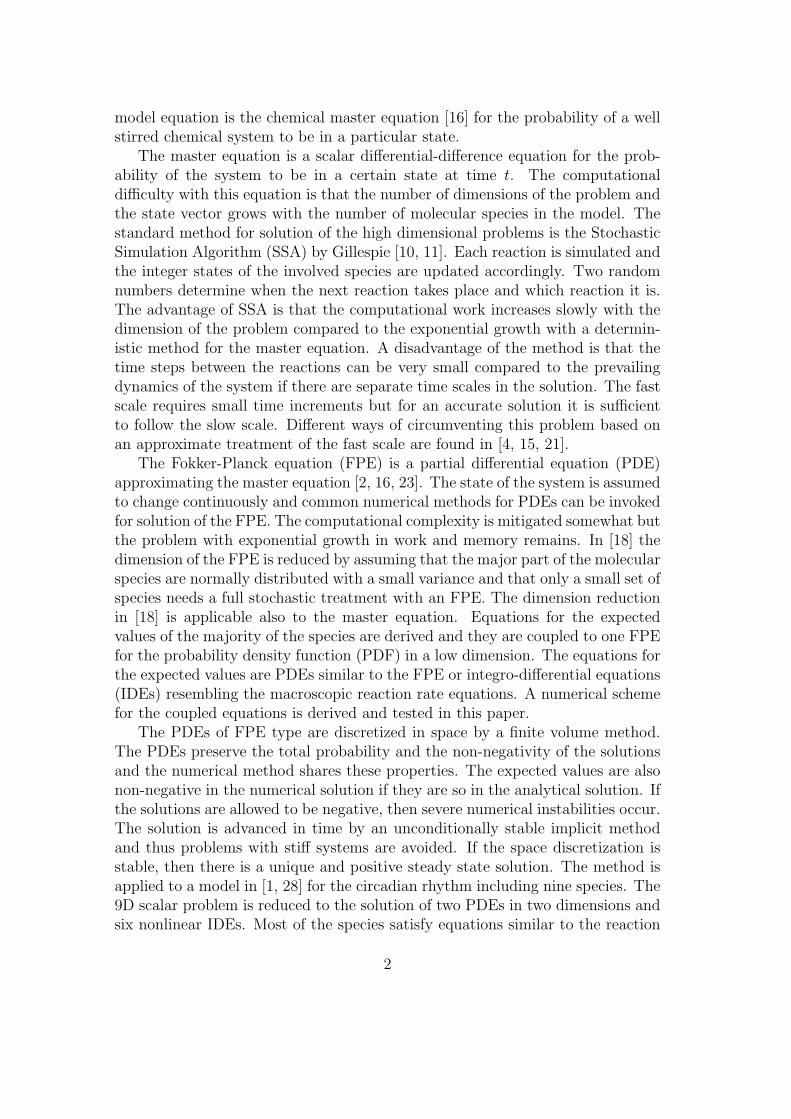
model equation is the chemical master equation [16] for the probability of a wellstirred chemical system to be in a particular state.

The master equation is a scalar differential-difference equation for the prob-ability of the system to be in a certain state at time t. The computationaldifficulty with this equation is that the number of dimensions of the problem andthe state vector grows with the number of molecular species in the model. Thestandard method for solution of the high dimensional problems is the StochasticSimulation Algorithm (SSA) by Gillespie [10, 11]. Each reaction is simulated andthe integer states of the involved species are updated accordingly. Two randomnumbers determine when the next reaction takes place and which reaction it is.The advantage of SSA is that the computational work increases slowly with thedimension of the problem compared to the exponential growth with a determin-istic method for the master equation. A disadvantage of the method is that thetime steps between the reactions can be very small compared to the prevailingdynamics of the system if there are separate time scales in the solution. The fastscale requires small time increments but for an accurate solution it is sufficientto follow the slow scale. Different ways of circumventing this problem based onan approximate treatment of the fast scale are found in [4, 15, 21].

The Fokker-Planck equation (FPE) is a partial differential equation (PDE)approximating the master equation [2, 16, 23]. The state of the system is assumedto change continuously and common numerical methods for PDEs can be invokedfor solution of the FPE. The computational complexity is mitigated somewhat butthe problem with exponential growth in work and memory remains. In [18] thedimension of the FPE is reduced by assuming that the major part of the molecularspecies are normally distributed with a small variance and that only a small set ofspecies needs a full stochastic treatment with an FPE. The dimension reductionin [18] is applicable also to the master equation. Equations for the expectedvalues of the majority of the species are derived and they are coupled to one FPEfor the probability density function (PDF) in a low dimension. The equations forthe expected values are PDEs similar to the FPE or integro-differential equations(IDEs) resembling the macroscopic reaction rate equations. A numerical schemefor the coupled equations is derived and tested in this paper.

The PDEs of FPE type are discretized in space by a finite volume method.The PDEs preserve the total probability and the non-negativity of the solutionsand the numerical method shares these properties. The expected values are alsonon-negative in the numerical solution if they are so in the analytical solution. Ifthe solutions are allowed to be negative, then severe numerical instabilities occur.The solution is advanced in time by an unconditionally stable implicit methodand thus problems with stiff systems are avoided. If the space discretization isstable, then there is a unique and positive steady state solution. The method isapplied to a model in [1, 28] for the circadian rhythm including nine species. The9D scalar problem is reduced to the solution of two PDEs in two dimensions andsix nonlinear IDEs. Most of the species satisfy equations similar to the reaction

2

rate equations and only a few are modeled stochastically. This is an examplewhere the macroscale model fails to reproduce the dynamics of the system. Theresult is sensitive to a parameter in the model. When it has a high value, then oursystem of equations and the reaction rate equations both exhibit an oscillatorybehavior. With a low value, the macroscopic model terminates at a fixed pointwhile the partly stochastic model continues to oscillate.

The outline of the paper is as follows. In the next section, the reduced systemof equations from [18] is given. The equations are discretized in space and timeand the boundary conditions are stated in Section 3. The properties of thediscrete solution are compared to the properties of the analytical solution inSection 4. The equations for the reduced stochastic model for the molecular clockin [1, 28] are solved in Section 5 and compared to the solution of the reactionrate equations. Finally, conclusions are drawn in the last section.

The i:th element of a vector v is denoted by vi. If vi ≥ 0 for all i, then wewrite v ≥ 0. The `p-norm of v of length N then is ‖v‖p = (

∑Ni=1 |vi|p)1/p in the

paper.

2 The system of equations

With N chemically active molecular species Xi, i = 1, . . . , N , xi denotes thenumber of molecules of substrate Xi. The state vector of the chemical system isx. A reaction r is a transition from a state xr to x so that xr = x + nr. Thereis a non-negative propensity wr(xr, t) for the probability of the reaction to occurper unit time. The reaction r can now be written

xrwr(xr,t)−−−−→ x, nr = xr − x. (1)

The time evolution of the state of the chemical system is governed by themaster equation [16]. The master equation is a differential-difference equationfor the PDF p(x, t) for the system to be in the state x at time t. The PDF isnon-negative for all x and t. The FPE is a PDE for p approximating the masterequation [16, 23] for x ∈ RN

+ , the non-negative N -dimensional orthant, and t ≥ 0.In [18], the state vector is split into two parts xT → (xT ,yT ) with x ∈ Rm

+ andy ∈ Rn. The transition vector nr for reaction r is split in the same manner nT

r →(mT

r ,nTr ) with mr ∈ Zm

+ , nr ∈ Zn+, where Z+ denotes the non-negative integer

numbers. The corresponding sets of stochastic variables are Xi, i = 1, . . . , m, andYi, i = 1, . . . , n. The assumption is that given X = x the stochastic variables Yi

are mutually independent and normally distributed with a small variance. ThePDF of the full system is

p(x,y, t) = (2σ2π)−n/2p0(x, t) exp(−n∑

j=1

(yj − φj)2

2σ2), x ∈ Rm

+ , y ∈ Rn. (2)

3

Assuming that the variance σ in (2) is small, a PDE is derived in [18] for thefirst partial moment for yk with respect to y. This moment is

pk(x, t) =

∫

Rn

ykp(x,y, t) dy = p0(x, t)φk(x, t). (3)

The conditional expected value of yk is φk since

E[yk|x] = pk(x, t)/p0(x, t) = φk(x, t). (4)

The PDE for pk is a FPE with a source term

∂pk(x, t)

∂t=

R∑r=1

∇ · Frk −R∑

r=1

nrkwr(x,φ(x, t), t)p0(x, t), (5)

for a chemical system with R reactions, where Frk is defined by

Frki = mri(qrk + 0.5mr · ∇qrk), i = 1, . . . , m, k = 1, . . . , ν, r = 1, . . . , R,

and qrk(x, t) = wr(x, φ, t)pk(x, t).If the difference between φk and its expected value

φk =

∫

Rm+

φk(x, t)p0(x, t) dx =

∫

Rm+

pk(x, t) dx =

∫

Rn

∫

Rm+

ykp(x,y, t) dxdy (6)

is small for k > ν, then an IDE is derived in [18] for φk, k = ν + 1, . . . , n,

dφk

dt= −

R∑r=1

nrk

∫

Rm+

wr(x,φ(x, t), t)p(x, t) dx. (7)

Now φ is defined by

φT = (φ1(x, t), . . . , φν(x, t), φν+1(t), . . . , φn(t)).

The shift in x by mr is ignored in (5) and (7) compared to the version in [18].The reaction rate equations corresponding to (7) are a system of nonlinear

ordinary differential equations (ODEs)

dφk

dt= −

R∑r=1

nrkwr(φ(t), t). (8)

The FPE for p0 is

∂p0(x, t)

∂t=

R∑r=1

m∑

i=1

mri∂qr(x, t)

∂xi

+ 0.5m∑

i=1

m∑j=1

mrimrj∂2qr(x, t)

∂xi∂xj

, (9)

4

with qr(x, t) = wr(x, φ, t)p0(x, t). This is a PDE to be solved for the scalar p0

in m dimensions. The number of dimensions m should be kept small so that theproblem is computationally tractable. Alternatively, the equation for p0 can bewritten

∂p0(x, t)

∂t=

R∑r=1

(mr · ∇)(qr + 0.5(mr · ∇)qr)

=R∑

r=1

0.5wr(mr · ∇)2p0 + (wr + (mr · ∇)wr)(mr · ∇)p0

+p0(mr · ∇)(wr + 0.5(mr · ∇)wr).

(10)

The same FPE in conservation form is

∂p0(x, t)

∂t=

R∑r=1

∇ · Fr = ∇ · F, (11)

with the flux functions

Fri = mri(qr + 0.5mr · ∇qr), i = 1, . . . , m, r = 1, . . . , R.

The boundary conditions at xi = 0, i = 1, . . . , N , are

Fi =R∑

r=1

Fri =R∑

r=1

mri(p0(wr + 0.5(mr · ∇)wr) + 0.5wr(mr · ∇)p0) = 0. (12)

The equations (5) and (9, 10, 11) are solved numerically in Ωh, where Ωh =x | 0 < xi < xmax is an open domain and xmax is so large that p ≈ 0 and∇p ≈ 0 in the neighborhood of xi = xmax for all i. If p = 0 and ∇p = 0 atxi = xmax for all i, then condition (12) is also satisfied there. The FPE (11) andthe boundary conditions imply that the total probability for p0

P0(t) =

∫

Ωh

p0(x, t) dx (13)

is constant for t ≥ 0, see [8].

3 Discretization of the Fokker-Planck equation

In order to conserve the total probability, the FPEs in conservation form in(5) and (11) are discretized by a finite volume method in space. The grid isCartesian covering Ωh with cells ω. The trapezoidal method (or Crank-Nicolsonmethod) advances the solution in time from tl to tl+1 with the time step ∆t. Thecoefficients in the difference stencil are such that the non-negativity of the PDFis preserved.

5

3.1 Space discretization

The space operator in (5) and (9) is written with p = p0 or p = pk

∇ ·∑Rr=1 Fr =

m∑i=1

∂

∂xi

(R∑

r=1

mriwr

)p + 0.5

m∑i=1

∂

∂xi

(R∑

r=1

m∑j=1

mrimrj∂wrp

∂xj

)

= ∇ ·G + 0.5∇ ·H,

(14)

where

Gi =

(R∑

r=1

mriwr

)p, Hi =

R∑r=1

Hri =R∑

r=1

m∑j=1

mrimrj∂wrp

∂xj

. (15)

The FPE is integrated over a cell ω and the time interval [tl, tl+1]

∫ tl+1

tl

∫

ω

∂p

∂tdω dt =

∫ tl+1

tl

∫

ω

∇ ·G + 0.5∇ ·H dω dt. (16)

The average p of p in ω satisfies

pl+1 − pl = |ω|−1

∫ tl+1

tl

∫

ω

∇ ·G + 0.5∇ ·H dω dt, (17)

where |ω| is the area of ω.The formulas are simplified if the approximations are derived for two space

dimensions, m = 2, and a constant step size, but the generalizations to higherdimensions and variable step sizes are straightforward. The integral form of (14)is taken over a square cell ωij with edge length h with midpoint at (x1ij, x2ij)and corners at (x1ij ± h/2, x2ij ± h/2). The four faces of ωij are denoted in thecounterclockwise direction by ∂ω1ij(where x1 = x1ij+h/2), ∂ω2ij(x2 = x2ij+h/2),∂ω3ij(x1 = x1ij − h/2), and ∂ω4ij(x2 = x2ij − h/2). Then

∫

ωij

∇ ·G + 0.5∇ ·H dω =∫

∂ω1ij

G1 + 0.5H1 dx2 −∫

∂ω3ij

G1 + 0.5H1 dx2

+

∫

∂ω2ij

G2 + 0.5H2 dx1 −∫

∂ω4ij

G2 + 0.5H2 dx1

(18)

by Gauss’ integral formula. We need evaluations of Gi + 0.5Hi on the four edgesof the cell in a finite volume discretization.

Let wi =∑

r mriwr, i = 1, 2, and let pij be the approximation of p in cell ωij.Then G is approximated as follows at x1 = x1ij + h/2

G1 = w1p ≈

w1,i+1/2,j pi+1,j, w1,i+1/2,j ≥ 0,w1,i+1/2,j pij, w1,i+1/2,j < 0,

(19)

6

and at x2 = x2ij + h/2

G2 = w2p ≈

w2,i,j+1/2 pi,j+1, w2,i,j+1/2 ≥ 0,w2,i,j+1/2 pij, w2,i,j+1/2 < 0,

(20)

where

w1,i+1/2,j = w1(xi+1/2,j,φ(xi+1/2,j, t), t), xi+1/2,j = xij + (h/2, 0)T ,w2,i,j+1/2 = w2(xi,j+1/2,φ(xi,j+1/2, t), t), xi,j+1/2 = xij + (0, h/2)T .

The flux G at x1 = x1ij − h/2 and x2 = x2ij − h/2 is determined in the samemanner. After division by the area |ω| = h2 of the cell, the first derivatives in thefirst sum in (14) are discretized by a first order accurate upwind approximationdepending on the sign of wi on the face between two cells.

The second derivatives are computed as follows for |mri| ≤ 1. In two dimen-sions, the Hr-fluxes are

Hr1 = m2r1

∂qr

∂x1

+ mr1mr2∂qr

∂x2

, Hr2 = mr1mr2∂qr

∂x1

+ m2r2

∂qr

∂x2

.

Let sr = mr1mr2 and let cij be values in the corners of the cell defined by

ci+1/2,j+1/2 =

qr,i+1,j+1 − qrij, sr = 1,qr,i+1,j − qr,i,j+1, sr = −1,

(21)

where qrij = wr(xij, φ(xij, t), t)pij = wrijpij. Then Hrk, k = 1, 2, at ∂ω1ij and∂ω2ij is approximated by

Hr1,i+1/2,j ≈

0, mr1 = 0,h−1(qr,i+1,j − qrij), mr2 = 0,0.5h−1(ci+1/2,j+1/2 + ci+1/2,j−1/2), |mr1| = |mr2| = 1,

Hr2,i,j+1/2 ≈

h−1(qr,i,j+1 − qrij), mr1 = 0,0, mr2 = 0,0.5h−1sr(ci+1/2,j+1/2 + ci−1/2,j+1/2), |mr1| = |mr2| = 1.

(22)

For cell ωij and |sr| = 1, the sum of the four integrated H-fluxes for reaction r is

0.5h−1( ci+1/2,j+1/2 + ci+1/2,j−1/2 − ci−1/2,j+1/2 − ci−1/2,j−1/2

+srci+1/2,j+1/2 − srci+1/2,j−1/2 + srci−1/2,j+1/2 − srci−1/2,j−1/2)= 0.5h−1( (1 + sr)ci+1/2,j+1/2 − (1 + sr)ci−1/2,j−1/2

+(1− sr)ci+1/2,j−1/2 − (1− sr)ci−1/2,j+1/2).

After division by the area of ωij, the resulting formula is

|ωij|−1

∫

ωij

∇ ·Hr dω ≈

h−2(qr,i+1,j+1 − 2qrij + qr,i−1,j−1), sr = 1,h−2(qr,i+1,j−1 − 2qrij + qr,i−1,j+1), sr = −1.

7

(23)

Regarded as a finite difference method for the PDF pij at the midpoints ina cell, the approximations (19), (20), of the first derivatives in (5) and (9) on agrid with constant grid size h is first order accurate and in two dimensions

∂wkp

∂xi

≈

h−1(wk,i+1/2,jpi+1,j − wk,i−1/2,jpij), wk,i+1/2,j, wk,i−1/2,j ≥ 0,h−1(wk,i+1/2,jpij − wk,i−1/2,jpi−1,j), wk,i+1/2,j, wk,i−1/2,j < 0,h−1(wk,i+1/2,jpi+1,j − wk,i−1/2,jpi−1,j), wk,i+1/2,j ≥ 0, wk,i−1/2,j < 0,h−1(wk,i+1/2,j − wk,i−1/2,j)pij, wk,i+1/2,j < 0, wk,i−1/2,j ≥ 0.

(24)

The coefficients multiplying pkl are non-negative except for the cell in the centerwhich has a non-positive coefficient. The second derivatives multiplied by thecoefficents mrimrj in (9) are approximated as in (22), (23), by

2∑i,j=1

mrimrj∂2wrp

∂xi∂xj

≈

h−2(wr,i+mri,j+mrjpi+mri,j+mrj

− 2wrijpij + wr,i−mri,j−mrjpi−mri,j−mrj

).

(25)

This is a second order accurate approximation of the sum also when |mri| or |mrj|is greater than one. If wr ≥ 0, then all coefficients in the stencil multiplying pkl

are non-negative except for pij in ωij.The integral of the source term in (5) is the expected value of wr in ωij. It is

approximated by the rectangle rule∫

ωij

wr(x, φ(x, t), t)p0(x, t) dω ≈ |ωij|wr(xij,φ(xij, t), t)p0ij. (26)

The integral in (7) is obtained by summing over all cells in (26).

3.2 Boundary conditions and conservation

Consider one rectangular cell ωij in the grid of length hi in the x-direction and hj

in the y-direction. The integral of the space operator over ωij is written accordingto the approximations above

|ωij|−1

∫

ωij

∇ ·G + 0.5∇ ·H dω =

h−1i (F1,i+1/2,j − F1,i−1/2,j) + h−1

j (F2,i,j+1/2 − F2,i,j−1/2),

with Fk,i,j = (Gk +0.5Hk)ij and i, j = 1, . . . , L. In the boundary cells of the com-putational domain, the total flux G+0.5H is zero at a cell face on the boundaryaccording to the boundary conditions of the differential equation (12). At the

8

left and right boundaries of the domain, e.g. at x1 = 0 we have F1,1/2,j = 0, andat x1 = xmax, F1,L+1/2,j = 0. The area weighted sum of the spatial approximationover all cells vanishes

L∑i=1

L∑j=1

|ωij|h−1i (F1,i+1/2,j − F1,i−1/2,j) + h−1

j (F2,i,j+1/2 − F2,i,j−1/2) =

L∑j=1

hj(F1,L+1/2,j − F1,1/2,j) +L∑

i=1

hi(F2,i,L+1/2 − F2,i,1/2) = 0

(27)

thanks to the conservative formulation and the boundary conditions. This prop-erty is shared by the analytical solution in (11) since

∫

Ωh

∇ · F dΩ =

∫

∂Ωh

F · nΩ dS = 0,

where ∂Ωh is the boundary of Ωh and nΩ is the normal of ∂Ωh (cf. (13)).The approximation in a cell at the left boundary in a two-dimensional domain

requires one extra numerical condition in a column of ghost cells with index i = 0.The space operator in ω1j is

F1,3/2,j + F2,1,j+1/2 − F2,1,j−1/2

= G1,3/2,j + G2,1,j+1/2 −G2,1,j−1/2 + 0.5(H1,3/2,j + H2,1,j+1/2 −H2,1,j−1/2).

The evaluations of Grk and Hrk when sr = 0 for reaction r pose no problem atthe boundary but for sr 6= 0 we have

Hr1,3/2,j + Hr2,1,j+1/2−Hr2,1,j−1/2 =

c3/2,j+1/2 − 0.5c1/2,j−1/2 + 0.5c1/2,j+1/2

when sr = 1,c3/2,j−1/2 − 0.5c1/2,j+1/2 + 0.5c1/2,j−1/2

when sr = −1.

By letting qr0j = qr1j in the ghost cell, the stencil in (23)

|ω1j|−1

∫

ω1j

∇ ·Hr dω ≈

h−2(qr,2,j+1 − 2qr1j + 0.5(qr,1,j+1 + qr,1,j−1))when sr = 1,h−2(qr,2,j−1 − 2qr1j + 0.5(qr,1,j+1 + qr,1,j−1))when sr = −1.

(28)

The other boundaries are treated in the same manner. If wr ≥ 0, then allcoefficients in the stencil multiplying pkl are non-negative also at the boundariesexcept for p1j in ω1j.

A generalization of the approximations (22) to the case when |mri|, |mrj| > 1,is possible, but the treatment of the boundaries and conservation of the totalprobability is more complicated. The resulting stencil in the interior of the do-main is still given by (25).

9

3.3 Time discretization

The mean values of p0 and pk, k = 1, . . . , ν, in the cells and the mean valuesφk, k = ν + 1, . . . , n, in Ωh are advanced in time by the trapezoidal method [14]applied to (11), (5), and (7).

Let µ be a multi-index such that µ = (µ1, µ2, . . . , µm). Then pliµ, i = 0, 1, . . . , ν,

approximates the mean value of pi(x, tl) in cell ωµ. The solution vector pli consists

of pliµ in some order. After time discretization, (11) is

pl+10 − pl

0 = 0.5∆t(Al+1pl+10 + Alpl

0), (29)

where Al is a sparse matrix representing the space discretization in Section 3.1and depends on xµ, φ

l, and tl. Since φk(x, t) = pk(x, t)/p0(x, t), the elements ofAl depend nonlinearly on pl

0 and plk. In cell µ, φl

kµ is computed by

φlkµ = φk(xµ, t

l) = plkµ/p

l0µ. (30)

Introduce the diagonal matrix Blk defined by

(Blkp

l0)µ =

R∑r=1

nrkwr(xµ,φlµ, t), t)p

l0µ. (31)

Then (5) for k = 1, . . . , ν, is approximated in time by

pl+1k − pl

k = 0.5∆t(Al+1pl+1k + Alpl

k)− 0.5∆t(Bl+1k pl+1

0 + Blkp

l0). (32)

The matrix Al multiplying pl0 in (29) and pl

k in (32) is the same. Also Blk depends

in a nonlinear way on pl0 and pl

k.The areas of the cells |ωµ| are collected in the vector ω in the same order as

in p0. Then the discretization of the IDEs (7) is

φl+1k − φl

k = −0.5∆t(ωT Bl+1k pl+1

0 + ωT Blkp

l0) (33)

for k = ν + 1, . . . , n, using the rectangle rule (26). By conservation (27) (seealso [8]), ωT Al = 0 for all l. With φl

k = ωTplk we find that (33) is obtained

by multiplying (32) from the left by ωT . These operations correspond on theanalytical side to the integration in (6) and the integration of (5) to arrive at (7).

The total discrete probability of p0 is (cf. (13))

P l+10 = ωTpl+1

0 = ωT (pl0 + 0.5∆t(Al+1pl+1

0 + Alpl0)) = ωTpl

0 = P l0 = P 0

0 ,

(34)

by (29) and conservation. The total discrete probability in (34) and the totalprobability in (13) share the same property: conservation over time. The totaldiscrete probability of pl+1

k is ωTpl+1k and satisfies (33).

10

The nonlinear system of equations to be solved for pl+10 ,pl+1

k , k = 1, . . . , ν,and φl+1

k , k = ν + 1, . . . , n, is with C l+1 = I − 0.5∆tAl+1

C l+1 0 . . .0.5∆tBl+1

1 C l+1 . . . 0...

. . .

0.5∆tBl+1ν 0 . . . C l+1 0 . . .

0.5∆tωT Bl+1ν+1 0 . . . 0 1 . . . 0

......

.... . .

0.5∆tωT Bl+1n 0 . . . 0 0 . . . 1

pl+10

pl+11...

pl+1ν

φl+1ν+1...

φl+1n

= bl, (35)

where the right hand side bl depends on the solution at tl. The equations (35) aresolved by a Newton-Krylov method [17] with GMRES [24] as the basic iterativemethod. With L cells in each coordinate direction, the number of unknowns isLm(ν+1)+(n−ν). The original N -dimensional problem with the same discretiza-tion has Lm+n unknowns. A reduction by about L−n has been accomplished.

4 Properties of the solutions

If there is a negative component of φ in wr(x,φ, t), wr may become negative forsome r and there is a risk of a severe instability in the numerical solution. Sinceφ is determined by φk and pk and p0 in (30), it is important to preserve the non-negativity of the solutions pk and φk of (32) and (33) and the positivity of p0 in(29). The analytical solutions of (5), (11), and (7) have these properties undercertain conditions. Sufficient conditions are derived for the numerical solutionsto be non-negative and positive too.

Other algorithms to maintain the non-negativity of solutions of ODEs arediscussed in [25]. One alternative there if the sign constraint on the solution isviolated is to halve the time step and recompute the solution. The convection-diffusion-reaction equation in one dimension is solved in [19] with finite differenceand finite element methods. Bounds are derived on the time step and the Courantnumber for positive solutions. A scalar hyperbolic PDE in one dimension issolved in [3] with a finite element method. By choosing the coefficients in thespace discretization depending on the solution, it remains positive. We will showhere that our scheme in Section 3 also preserves non-negativity and positivity bytaking sufficiently small time steps. The alternative in [25] to reset the negativevariable to zero is not satisfactory for p0. By letting pl

0µ := max(ε, pl0µ), φl

kµ

depends critically on the choice of ε > 0.Consider equations (11), (5), and (7) separate from each other without the

coupling via φ and p0. Let

wk(x,φ, t) = −∑

r

nrkwr(x,φ, t) (36)

11

and assume that wk and φ are in C1 with respect to the independent variables.Then we have the following result for the analytical solution φk, k = ν +1, . . . , n,of (7).

Theorem 1. Assume that for k = ν + 1, . . . , n, and t ≥ 0

wk(x, φ1, . . . , φν , φν+1, . . . , φk−1, 0, φk+1, . . . , φn, t) ≥ 0, (37)

when φj ≥ 0, j 6= k, p0(x, t) ≥ 0, and that φk(0) ≥ 0. Then

φk(t) ≥ 0

when t > 0.

Proof. Let wk(φ, t) =

∫

Rm+

wk(x,φ, t)p0(x, t) dx. Then

wk(φ1, . . . , φν , φν+1, . . . , φk−1, 0, φk+1, . . . , φn, t) ≥ 0.

If at some instance t0 we have φk(t0) = 0, then in (7) dφk/dt = wk ≥ 0 and φk

can never cross the boundary φk = 0 and become negative. ¥

For the numerical solution of (7) we have a similar result.

Theorem 2. Assume that (37) is satisfied, pl0 ≥ 0 for all l, and that φ0

k > 0for k = ν + 1, . . . , n. Let ∆t be sufficiently small. Then

φlk > 0

when l > 0.

Proof. Assume that φl

> 0. Then compute φl+1

and we will show that

φl+1

> 0.Let wl

k = −ωT Blkp

l0 in (33). For φl+1

k in (7) we have that

φl+1k = φl

k + 0.5∆twl+1k (φ

l+1) + 0.5∆twl

k(φl).

There is a bound ∆t1 such that φlk + 0.5∆twl

k(φl) > 0 when ∆t ≤ ∆t1 since

φlk > 0, wl

k ∈ C1, and wlk(φ

l1, . . . , φ

lk−1, 0, φ

lk+1, . . .) ≥ 0.

Consider the index set K consisting of all k such that |φl+1k | ≤ ε for some small

ε > 0 for which there is a risk that φl+1k is non-positive. Partition φ

l+1such that

φI consists of components with k ∈ K and φII holds the remaining components.

For wl+1k (φ

l+1), k ∈ K, we have the Taylor expansion about φ

l+1I = 0

wl+1I (φ

l+1) = wl+1

0 (φl+1II ) + W l+1φ

l+1I ,

12

where W l+1ij depends on ∂wi/∂φj, see p. 190 in [5], and wl+1

0 ≥ 0. The solution

φl+1I satisfies

(D − 0.5∆tB)φl+1I = c,

where D = diag(1 − 0.5∆tW l+1jj ), Bii = 0, Bij = W l+1

ij when i 6= j, and c > 0.Thus,

φl+1I = (I − 0.5∆tD−1B)−1D−1c. (38)

If at least one W l+1jj is positive, then a bound ∆t2 = 2/ maxi max(W l+1

ii , 0) on

∆t guarantees that D is invertible and has positive diagonal elements. If all W l+1jj

are non-positive, then any positive ∆t is acceptable. Let ∆t3 < ∆t2 be such that

0.5∆t3‖D−1B‖∞ = 0.5∆t3 maxi|1− 0.5∆t3W

l+1ii |−1

∑

j,j 6=i

|W l+1ij | < 1.

The right hand side in (38) is

(I − 0.5∆tD−1B)−1D−1c = D−1c + ((I − 0.5∆tD−1B)−1 − I)D−1c, (39)

with D−1c > 0. For ∆t ≤ ∆t3 we have

‖(I − 0.5∆tD−1B)−1 − I‖∞ ≤∑∞j=1 0.5j∆tj‖D−1B‖j

∞ = 0.5∆t‖D−1B‖∞/(1− 0.5∆t‖D−1B‖∞).

Choose ∆t4 ≤ ∆t3 such that

0.5∆t4‖D−1B‖∞/(1− 0.5∆t4‖D−1B‖∞)‖D−1c‖∞ < minj

(D−1c)j.

Then the expression in (39) is positive. Therefore, if ∆t ≤ min(∆t1, ∆t4) thenφl+1 > 0 in (38) and the theorem is proved. ¥

The equations (5) for pk and (10) for p0 are investigated by means of themaximum principle for parabolic equations to show that a positive initial solutionwill remain positive in a finite interval (0, T ]. Let M(x, t) ∈ Rm×m have theelements

Mij =R∑

r=1

mrimrjwr(x, φ, t)

so that the second order term in (5) and (10) can be written

0.5m∑

i,j=1

Mij∂2p

∂xi∂xj

13

with p = p0 or p = pk. Then we have

Theorem 3. Assume that M is positive definite and that wr and φ are in C2

in Ωh × [0, T ] in their independent variables.If p0(x, t) ≥ 0 on the boundary ∂Ωh and the initial conditions are p0(x, 0) > 0

in Ωh, then p0(x, t) > 0 in Ωh × (0, T ].If pk(x, t) ≥ 0 on the boundary ∂Ωh, the initial conditions are pk(x, 0) > 0

in Ωh for k = 1, . . . , ν, p0(x, t) ≥ 0, and wk(x,φ, t) ≥ 0, then pk(x, t) > 0 inΩh × (0, T ].

Proof. The strong minimum principle on p. 122 in [22] is applicable withinfΩ×(0,T ] p = 0 since M is positive definite. If pj = 0, j = 0, 1, . . . , ν, somewherein Ωh × (0, T ] then pj = 0 everywhere, which contradicts the initial condition.Hence, p(x, t) > 0 in Ωh for t ∈ (0, T ]. ¥

Remark. A sufficient condition for M to be positive definite is that all wr arepositive in Ωh and that the stoichiometric matrix

S = (m1,m2, . . . ,mR) ∈ Rm×R

has rank m (see [26]). The propensities will be positive at least in Ωh if φ ispositive there.

The steady state solution of (11) satisfies an elliptic equation with Mij mul-tiplying the second derivatives and

c =R∑

r=1

(mr · ∇)(wr + 0.5(mr · ∇)wr) (40)

multiplying p0 in (10). If c ≤ 0, then the maximum (or minimum) principle on p.35 in [9] or p. 109 in [22] is applicable also to the steady state problem to showthat a solution will be positive in the interior of the domain.

The solutions of (29) and (32) have properties similar to those of the solutionsof (10) and (5).

Theorem 4. Assume that wlrµ = wr(xµ, φ

lµ, t

l) ≥ 0 for all l > 0 and that ∆tis sufficiently small.

If p00µ > 0 for every µ, then pl

0µ > 0.If p0

kµ > 0 for every µ and k = 1, . . . , ν, pl0µ ≥ 0, and wk(xµ, φ

lµ, t

l) ≥ 0, then

plkµ > 0.

Proof. From (29) and (32) we conclude that both pl+10 and pl+1

k satisfy

(1− 0.5∆tAii)pl+1i = 0.5∆t

∑

j 6=i

Aijpl+1j + c,

14

where A = Al+1,p = p0 or p = pk, and

c = (I + 0.5∆tAl)pl, if p = p0,c = (I + 0.5∆tAl)pl − 0.5∆t(Bl+1

k pl+10 + Bl

kpl0), if p = pk.

We will show by induction that if pl > 0 then pl+1 > 0.The elements of A are given by (24), (25), and Section 3.2. There is a ∆t1 such

that if ∆t ≤ ∆t1, then (I + 0.5∆tAl)ij ≥ 0. By the assumption on pl0 and wk we

have Blkp

l0 ≤ 0 for every l and therefore c > 0. If J is the set of cells neighboring

cell i, then |Aii−Aij| ≤ κh, j ∈ J , for some κ since wr ∈ C1 and Aij = 0 when jis outside J . Then there is a ∆t2 such that 0.5∆t

∑j Aij ≤ 1− 0.5∆tAii for all

i if ∆t ≤ ∆t2.Thus, in the interior and in the boundary cells pl+1

i satisfies

pl+1i > 0.5∆t

∑j

Aijpl+1j /(1− 0.5∆tAii) (41)

Assume that pl+1i = minµ pl+1

µ ≤ 0. Then the lowest value of the right hand side

in (41) is obtained by taking pl+1j = pl+1

i resulting in

pl+1i > (0.5∆t

∑j

Aij/(1− 0.5∆tAii))pl+1i ,

and we have a contradiction unless pl+1i > 0. Hence, if ∆t ≤ min(∆t1, ∆t2), then

pl+10 > 0 and pl+1

k > 0 and the theorem is proved. ¥

The steady state solution p∞0 of (29) satisfies

Ap∞0 = 0, (42)

where A = liml→∞ Al. There is one eigenvalue of A equal to zero with the righteigenvector p∞0 and the left eigenvector ω (see Section 3.3 and [8]). The propertiesof p∞0 are derived in the next theorem using Perron’s theory for positive matrices.The directed graph of a matrix A is defined by the elements of A. An L × Lmatrix has L vertices in the graph and an edge between the vertices i and j ifAij 6= 0. An irreducible matrix A has a directed graph where there is a chain ofedges between every pair of vertices in the graph (see [13]).

Theorem 6. With the space discretization in Section 3.1 assume that

liml→∞

wr(xµ,φlµ, t

l) = w∞rµ ≥ 0

and that all other eigenvalues of A except 0 satisfy <λ(A) < 0. Then p∞0 ≥ 0.If in addition A is irreducible, then there is only one λ(A) = 0 and p∞0 is uniqueand positive.

15

Proof. For a sufficiently small γ > 0, I + γA has non-negative elements andthe eigenvalue of largest modulus is 1. The corresponding eigenvector v is thePerron vector and fulfills v ≥ 0 according to p. 158 in [13]. We have Av = 0and p∞0 = v. If A is irreducible, then I + γA has the same property. If I + γAis irreducible and has another eigenvalue with modulus 1, then it is exp(iψ) forsome ψ 6= 0 with eigenvector v > 0 by the Perron-Frobenius theory (p. 159 in[13]). The corresponding λ(A) = (exp(iψ)− 1)/γ 6= 0 and λ(A) = 0 and p∞0 areunique. ¥

Remark. As an example, a sufficient condition in one dimension for ourmatrix A to be irreducible is w∞

rj 6= 0 for all j. With the condition on λ(A) inthe theorem, all solutions of the ODE system dp/dt = Ap vanish when t → ∞except for p∞0 . The condition on c in (40) and on λ(A) in the theorem are relatedin the following way: Decreasing c would shift the spectrum of A further into theleft half plane.

If the conditions in Theorem 3 are fulfilled, then by (13) p0 is constant in theL1-norm for t ≥ 0

‖p0(·, t)‖1 =

∫

Ωh

|p0(x, t)| dx =

∫

Ωh

p0(x, t) dx = P0(0).

The same property holds for pl0 in the `1-norm if the conditions in Theorem 4

are satisifed

‖pl0‖h,1 =

∑µ

|ωµ||pl0µ| =

∑µ

|ωµ|pl0µ = ωTp0

0 = P 00

according to (34).

5 Numerical results for the circadian rhythm

Living organisms have to adapt their behavior to different periodic changes intheir environment e.g. the daily variation of light and the annual variation oftemperature. Many of them have developed molecular clocks as their internaltime-keeping mechanisms. An example of such an oscillatory process is the cir-cadian rhythm with a period of about 24 h [12]. A model for this rhythm hasbeen developed in [1] and is simplified in [28]. The reactions in this model aresimulated here using the numerical method developed in the previous sections.With a particular choice of a parameter the macroscopic and deterministic modelimmediately arrives at a steady state solution but the mesoscopic and stochasticmodel continues to oscillate.

Consider the following 18 reactions for the nine molecular species

16

A,C,R, Da, D′a, Dr, D

′r,Ma,M

′a modeling the circadian rhythm:

D′a

θaD′a−−−→ Da

Da + AγaDaA−−−−→ D′

a

D′r

θrD′r−−−→ Dr

Dr + AγrDrA−−−−→ D′

r

∅ α′aD′a−−−→ Ma

∅ αaDa−−−→ Ma

MaδmaMa−−−−→ ∅

∅ βaMa−−−→ A

∅ θaD′a−−−→ A

∅ θrD′r−−−→ A

AδaA−−→ ∅

A + RγcAR−−−→ C

∅ α′rD′r−−−→ Mr

∅ αrDr−−−→ Mr

MrδmrMr−−−−→ ∅

∅ βrMr−−−→ R

RδrR−−→ ∅

CδaC−−→ R

(43)

The reaction constants are found in Table 1. The parameter δr will have twodifferent values 0.2 and 0.08 in the numerical experiments.

αa 50 βa 50 γa 1 δma 10 θa 50α′a 500 βr 5 γr 1 δmr 0.5 θr 100αr 0.01 γc 2 δa 1α′r 50 δr -

Table 1: Parameters of the circadian clock (43).

Without any assumptions on the distributions of the molecular species, theFPE for (43) is a scalar PDE in nine dimensions for the PDF p with m = 9, ν =0, n = 0. The computational complexity of the problem is reduced in two ways:

1. Complex C and repressor R are stochastic variables, the remaining specieshave normal distributions with a small σ, activator A has a variable φA(x, t)while the other expected values φk are only dependent on time ⇒ 2 PDEsin 2D, 6 IDEs (m = 2, ν = 1, n = 7).

2. All species have normal distributions with small σ ⇒ reaction rate equations(8), 9 ODEs (m = 0, ν = 0, n = 9).

In the first case, (11) determines p0, (5) is solved for p1 = pA and φA(x, t),and the expected values for the remaining six species satisfy (7). In the secondcase, the equations are solved with the ODE integrator ode15s from MATLAB.

The initial values at t = 0 are Da(0) = 0.1, Dr(0) = 0.1, D′a(0) = 0.1, D′

r(0) =0.1,Ma(0) = 0.1,Mr(0) = 0.1. After a short transient phase, the variables areadjusted so that the solution is in the periodic regime. The expected value φA is0.1 initially and

p0(x, 0) =1

2π · 720exp

(−(x1 − 90)2 + (x2 − 90)2

2 · 720

).

17

The chemical system with δR = 0.2 is simulated in Figures 1 and 2 usingthe two modeling alternatives. The solution is computed with the reaction rateequations and displayed for the D and M variables in Figure 1. The solution withthe stochastic model is similar. In Figure 2, the expected values of the complexand the repressor are compared to the solutions with the reaction rate equations.The periods with the two methods are almost the same with the ODE solutionlagging slightly behind. Both solutions are oscillatory.

0 25 500

0.1

0.2

time

D

0 25 500

5

10

time

M

(a) (b)

Figure 1: The solution is obtained by solving the ODEs for δr = 0.2. The speciesDa (solid upper solution at t ≈ 1), Dr (dashed upper solution at t ≈ 1), D′

a (solidlower solution at t ≈ 1), and D′

r (dashed lower solution at t ≈ 1) are displayedin (a), and the species Ma (solid) and Mr (dashed) are displayed in (b).

0 25 500

200

400

time

C

0 25 500

200

400

time

R

(a) (b)

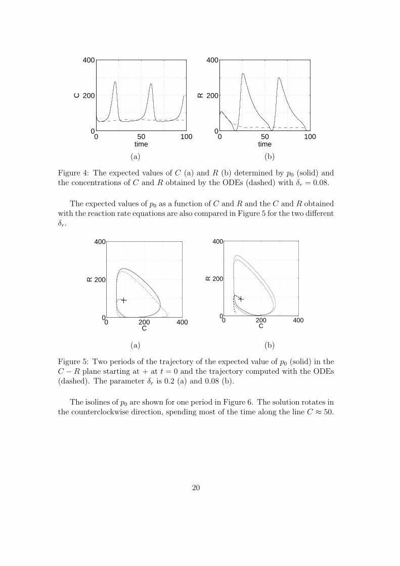
Figure 2: The expected values of C (a) and R (b) determined by p0 (solid) andthe concentrations of C and R obtained by the ODEs (dashed) with δr = 0.2.

The parameter δr is changed to 0.08 and the simulations are repeated with thesame inital data in Figures 3 and 4. There is no oscillation in the deterministic

18

model. The solution quickly reaches a stable fixed point but the noise in thestochastic model is sufficiently strong to permit an oscillatory solution. This isin agreement with simulations in [28] using the SSA [10] and a method based onthe evolution of the moments in [7]. Our simplified model with 2 PDEs in 2Dand 6 IDEs captures the correct behavior of the original 9D problem.

0 50 1000

0.1

0.2

time

D

0 50 1000

5

10

timeM

0 50 1000

0.1

0.2

time

D

0 50 1000

5

10

time

M

(a) (b)

Figure 3: The solution is obtained by solving the IDEs (upper) and the ODEs(lower) for δr = 0.08. The species Da (solid upper solution at t ≈ 1), Dr (dashedupper solution at t ≈ 1), D′

a (solid lower solution at t ≈ 1), and D′r (dashed lower

solution at t ≈ 1) are displayed in column (a), and the species Ma (solid) and Mr

(dashed) are displayed in column (b).

19

0 50 1000

200

400

time

C

0 50 1000

200

400

time

R

(a) (b)

Figure 4: The expected values of C (a) and R (b) determined by p0 (solid) andthe concentrations of C and R obtained by the ODEs (dashed) with δr = 0.08.

The expected values of p0 as a function of C and R and the C and R obtainedwith the reaction rate equations are also compared in Figure 5 for the two differentδr.

0 200 4000

200

400

C

R

0 200 4000

200

400

C

R

(a) (b)

Figure 5: Two periods of the trajectory of the expected value of p0 (solid) in theC −R plane starting at + at t = 0 and the trajectory computed with the ODEs(dashed). The parameter δr is 0.2 (a) and 0.08 (b).

The isolines of p0 are shown for one period in Figure 6. The solution rotates inthe counterclockwise direction, spending most of the time along the line C ≈ 50.

20

0 200 400 6000

200

400

600time = 48.5451

C

R

0 200 400 6000

200

400

600time = 56.3123

C

R

0 200 400 6000

200

400

600time = 62.1377

C

R

0 200 400 6000

200

400

600time = 67.9631

C

R

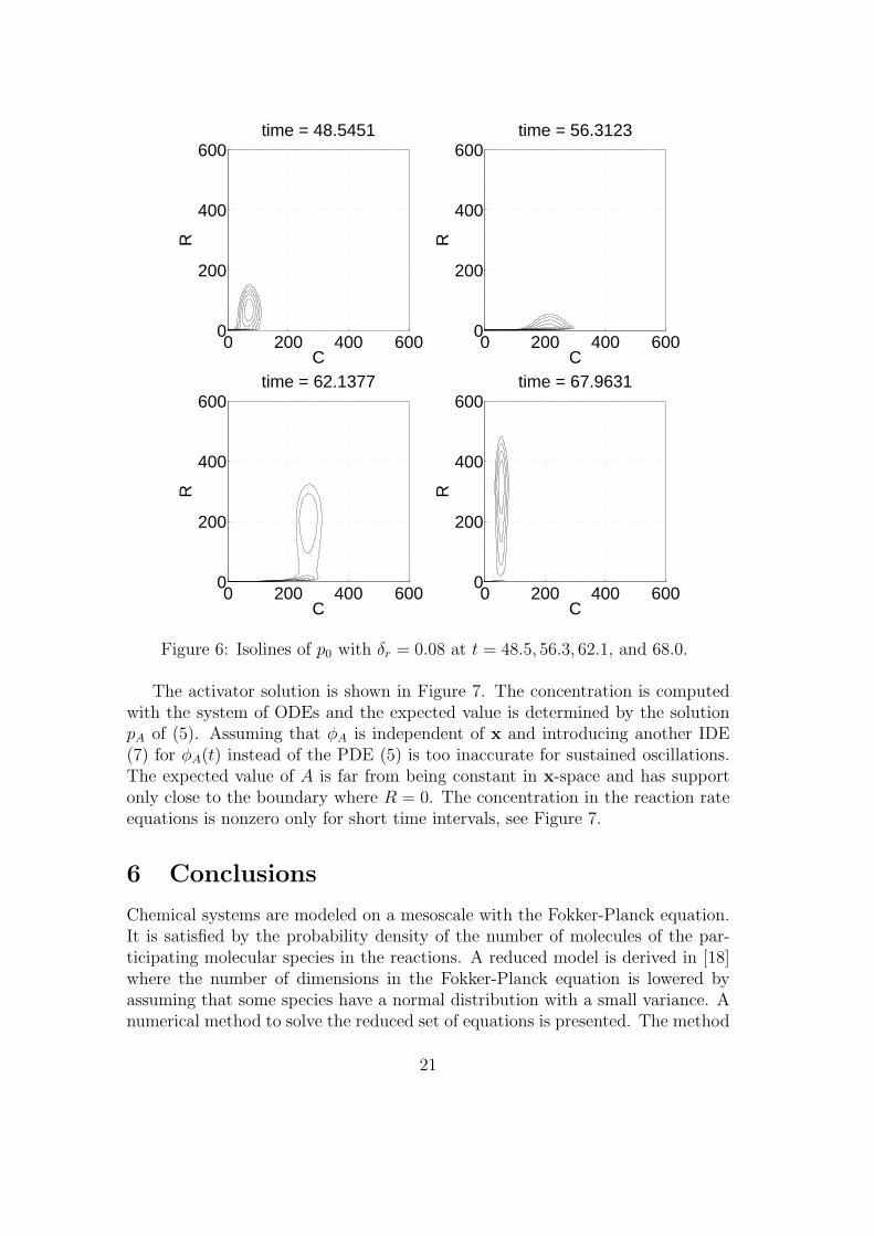
Figure 6: Isolines of p0 with δr = 0.08 at t = 48.5, 56.3, 62.1, and 68.0.

The activator solution is shown in Figure 7. The concentration is computedwith the system of ODEs and the expected value is determined by the solutionpA of (5). Assuming that φA is independent of x and introducing another IDE(7) for φA(t) instead of the PDE (5) is too inaccurate for sustained oscillations.The expected value of A is far from being constant in x-space and has supportonly close to the boundary where R = 0. The concentration in the reaction rateequations is nonzero only for short time intervals, see Figure 7.

6 Conclusions

Chemical systems are modeled on a mesoscale with the Fokker-Planck equation.It is satisfied by the probability density of the number of molecules of the par-ticipating molecular species in the reactions. A reduced model is derived in [18]where the number of dimensions in the Fokker-Planck equation is lowered byassuming that some species have a normal distribution with a small variance. Anumerical method to solve the reduced set of equations is presented. The method

21

preserves the total probability and the non-negativity of the solution, propertiesshared by the analytical solution. The scheme is applied to a chemical modelof a molecular clock commonly found in many organisms from bacteria to mam-mals. The oscillations are sensitive to a parameter in the model. If the parameteris sufficiently large then both the solutions from the macroscopic reaction rateequations and our reduced mixed macroscopic and mesoscopic model have an os-cillatory behavior. With a lower value, only the solution with our reduced modelcontinues to oscillate. This is in agreement with the conclusions in [28]. Further-more, the computational complexity has been reduced from nine dimensions inthe original problem to two dimensions.

0 25 500

100

200

300

time

A

0200

400600

0200

400600

0

100

200

C

R

A

(a) (b)

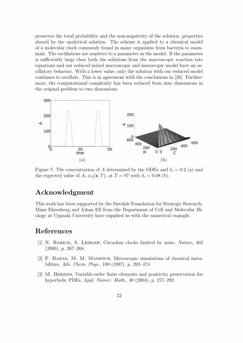
Figure 7: The concentration of A determined by the ODEs and δr = 0.2 (a) andthe expected value of A, φA(x, T ), at T = 97 with δr = 0.08 (b).

Acknowledgment

This work has been supported by the Swedish Foundation for Strategic Research.Mans Ehrenberg and Johan Elf from the Department of Cell and Molecular Bi-ology at Uppsala University have supplied us with the numerical example.

References

[1] N. Barkai, S. Leibler, Circadian clocks limited by noise, Nature, 403(2000), p. 267–268.

[2] F. Baras, M. M. Mansour, Microscopic simulations of chemical insta-bilities, Adv. Chem. Phys., 100 (1997), p. 393–474.

[3] M. Berzins, Variable-order finite elements and positivity preservation forhyperbolic PDEs, Appl. Numer. Math., 48 (2004), p. 271–292.

22

[4] Y. Cao, D. Gillespie, L. Petzold, Multiscale stochastic simulationalgorithm with stochastic partial equilibrium assumption for chemically re-acting systems, J. Comput. Phys., 206 (2005), p. 395–411.

[5] J. Dieudonne, Foundations of Modern Analysis, Academic Press, NewYork, 1969.

[6] J. Elf, J. Paulsson, O. G. Berg, M. Ehrenberg, Near-critical phe-nomena in intracellular metabolite pools, Biophys. J., 84 (2003), p. 154–170.

[7] S. Engblom, Computing the moments of high dimensional solutionsof the master equation, Technical report 2005-020, Dept of Informa-tion Technology, Uppsala University, Uppsala, Sweden, 2005, available athttp://www.it.uu.se/research/reports/2005-020/, to appear in Appl.Math. Comput.

[8] L. Ferm, P. Lotstedt, P. Sjoberg, Adaptive, conserva-tive solution of the Fokker-Planck equation in molecular biol-ogy, Technical report 2004-054, Dept of Information Technol-ogy, Uppsala University, Uppsala, Sweden, 2004, available athttp://www.it.uu.se/research/publications/reports/2004-054/.

[9] D. Gilbarg, N. S. Trudinger, Elliptic Partial Differential Equations ofSecond Order, Springer, Berlin, 1998.

[10] D. T. Gillespie, A general method for numerically simulating the stochas-tic time evolution of coupled chemical reactions, J. Comput. Phys., 22 (1976),p. 403–434.

[11] D. T. Gillespie, Exact stochastic simulation of coupled chemical reactions,J. Phys. Chem., 81 (1977), p. 2340–2361.

[12] A. Golbeter, Computational approaches to cellular rhythms, Nature, 420(2002), p. 238–245.

[13] A. Greenbaum, Iterative Methods for Solving Linear Systems, SIAM,Philadelphia, 1997.

[14] E. Hairer, S. P. Nørsett, G. Wanner, Solving Ordinary DifferentialEquations, 2nd ed., Springer-Verlag, Berlin, 1993.

[15] E. Haseltine, J. Rawlings, Approximate simulation of coupled fast andslow reactions for stochastic chemical kinetics, J. Chem. Phys., 117 (2002),p. 6959–6969.

[16] N. G. van Kampen, Stochastic Processes in Physics and Chemistry, North-Holland, Amsterdam, 1992.

23

[17] D. A. Knoll, D. E. Keyes, Jacobian-free Newton-Krylov methods: asurvey of approaches and applications, J. Comput. Phys., 193 (2004), p.357–397.

[18] P. Lotstedt, L. Ferm, Dimensional reduction of the Fokker-Planck equa-tion for stochastic chemical reactions, Technical report 2005-023, Dept of In-formation Technology, Uppsala University, Uppsala, Sweden, 2005, availableat http://www.it.uu.se/research/reports/2005-023/.

[19] R. J. MacKinnon, G. F. Carey, Positivity-preserving, flux-limited finite-difference and finite-element methods for reactive transport, Int. J. Numer.Meth. Fluids., 41 (2003), p. 151–183.

[20] H. H. McAdams, A. Arkin, It’s a noisy business. Genetic regulation atthe nanomolar scale, Trends Gen., 15 (1999), p. 65–69.

[21] C. V. Rao, A. P. Arkin, Stochastic chemical kinetics and the quasi-steady-state assumption: Application to the Gillespie algorithm, J. Chem.Phys., 118 (2003), p. 4999–5010.

[22] M. Renardy, R. C. Rogers, An Introduction to Partial Differential Equa-tions, Springer, New York, 1993.

[23] H. Risken, The Fokker-Planck Equation, 2nd ed., Springer, Berlin, 1996.

[24] Y. Saad, M. H. Schultz, GMRES: A generalized minimal residual algo-rithm for solving nonsymmetric linear systems, SIAM J. Sci. Stat. Comput.,7 (1986), p. 856–869.

[25] L. F. Shampine, S. Thompson, J. A. Kierzenka, G. D. Byrne, Non-negative solutions of ODEs, Appl. Math. Comput., 170 (2005), p. 556–569.

[26] P. Sjoberg, P. Lotstedt, J. Elf, Fokker-Planck approximation of themaster equation in molecular biology, Technical report 2005-044, Dept of In-formation Technology, Uppsala University, Uppsala, Sweden, 2005, availableat http://www.it.uu.se/research/reports/2005-044/.

[27] M. Thattai, A. van Oudenaarden, Intrinsic noise in gene regulatorynetworks, Proc. Nat. Acad. Sci., 98 (2001), p. 8614–8619.

[28] J. M. G. Vilar, H. Y. Kueh, N. Barkai, S. Leibler, Mechanisms ofnoise-resistance in genetic oscillators, Proc. Nat. Acad. Sci., 99 (2002), p.5988–5992.

24