UNIVERSITÀ DEGLI STUDI DI PADOVA

Department of Industrial Engineering

TECHNICAL UNIVERSITY OF DENMARK

DTU-MEK – Section of Fluid Mechanics, Costal and Maritime Engineering

Master of Science Degree in Mechanical Engineering

Numerical simulation of the in-nozzle flow during the opening

and closing of the fuel valve for two-stroke diesel engines

Supervisors: Prof. Giovanna Cavazzini

Università degli Studi di Padova

Prof. Jens Honoré Walther

Technical University of Denmark

Eng. Simon Matlok

MAN Energy Solutions

Master thesis by:

Lorenzo Zambon

1154346 – s171971

Academic year 2018-2019

Numerical simulation of in-nozzle flow during the opening and closing of a fuel valve for two-stroke diesel engines

Mas

ter T

hesi

s

Lorenzo Zambon

DTU Mechanical Engineering

Section of Fluid Mechanics, Costal and Maritime Engineering

Università degli Studi di Padova

Department of Industrial Engineering

June 2019

Abstract

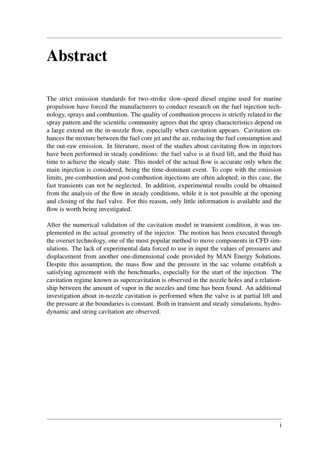
The strict emission standards for two-stroke slow-speed diesel engine used for marinepropulsion have forced the manufacturers to conduct research on the fuel injection tech-nology, sprays and combustion. The quality of combustion process is strictly related to thespray pattern and the scientific community agrees that the spray characteristics depend ona large extend on the in-nozzle flow, especially when cavitation appears. Cavitation en-hances the mixture between the fuel core jet and the air, reducing the fuel consumption andthe out-raw emission. In literature, most of the studies about cavitating flow in injectorshave been performed in steady conditions: the fuel valve is at fixed lift, and the fluid hastime to achieve the steady state. This model of the actual flow is accurate only when themain injection is considered, being the time-dominant event. To cope with the emissionlimits, pre-combustion and post-combustion injections are often adopted; in this case, thefast transients can not be neglected. In addition, experimental results could be obtainedfrom the analysis of the flow in steady conditions, while it is not possible at the openingand closing of the fuel valve. For this reason, only little information is available and theflow is worth being investigated.

After the numerical validation of the cavitation model in transient condition, it was im-plemented in the actual geometry of the injector. The motion has been executed throughthe overset technology, one of the most popular method to move components in CFD sim-ulations. The lack of experimental data forced to use in input the values of pressures anddisplacement from another one-dimensional code provided by MAN Energy Solutions.Despite this assumption, the mass flow and the pressure in the sac volume establish asatisfying agreement with the benchmarks, especially for the start of the injection. Thecavitation regime known as supercavitation is observed in the nozzle holes and a relation-ship between the amount of vapor in the nozzles and time has been found. An additionalinvestigation about in-nozzle cavitation is performed when the valve is at partial lift andthe pressure at the boundaries is constant. Both in transient and steady simulations, hydro-dynamic and string cavitation are observed.

i

ii

Abstract (Italian)

Le stringenti normative riguardo le emissioni di motori diesel a due tempi per la propul-sione navale ha incentivato la ricerca da parte dei costruttori; i principali ambiti di stu-dio rigurdano i combustibili, l’iniezione e il processo di combustione. L’efficienza diquest’ultima e associata allo spray pattern e l’atomizzazione del getto dipende in largamisura dal flusso del combustibile negli ugelli di iniezione, specialmente quando si hacavitazione. La cavitazione permette di migliorare la miscela di aria e combustibile,riducendo i consumi e le emissioni di incombusti. In letteratura, la maggior parte deglistudi rigurdanti la cavitazione negli iniettori e svolta in condizioni stazionarie: la valvoladell’iniettore e alla massima alzata, le condizioni di pressione sono tempo invarianti e ilfluido ha sufficiente tempo per raggiungere le condizioni stazionarie. Questo tipo di mod-ellizzazione fluidodinamica dell’iniezione risulta essere accurato quando la sola iniezioneprinicipale viene considerata, essendo questa la parte dominante dell’intero processo. Aseguito delle limitazioni sulle emissioni, pre e post iniezioni sono spesso utilizzate nellecondizioni operative; in questo casto, i transitori dovuti alla apertura e chiusura dellavalvola non possono essere ignorati. In aggiunta, nonostante le pressioni e le dimen-sioni degli ugelli rendano complesso l’approccio sperimentale, e possible effetturare degliesperimenti quando la valvola si trova alla massima alzata. Al contrario cio non e possi-bile nei transitori e dati sperimentali sono assenti in letteratura. Queste ragioni rendono lostudio del flusso di combustibile all’apertura e chiusura della valvola meritevole di appro-fondimento.

Dopo una validazione numerica delle equazioni responsabili del fenomeno di cavitazionein condizioni transitorie, queste sono state implementate in un modello CFD dell’iniettore.Il movimento della valvola e stato possibile grazie all’utilizzo della tecnologia overset, unodei metodi piu popolari per simulare il moto di componenti nei software CFD. La man-canza di dati sperimentali ha richiesto l’utilizzo in input di valori numerici derivanti daaltri strumenti monodimensionali. Nonostante questa assunzione, le portate di massa ela pressione nel volume di sac mostrano una corrispondenza con i valori di benchmark,specialmente per quanto concerne l’avvio dell’iniezione. Il regime di cavitazione noto inletteratura come supercavitation e stato osservato negli ugelli e una relazione tra l’alzatadello spillo e volume di vapore di combustibile e stata ricavata. Uno studio aggiuntivo rig-urdo il fenomeno di cavitazione negli ugelli in condizioni stazionarie e ad alzate parzialidello spillo e stata effettuato. Sia nelle simulazioni transitorie che in quelle in condizionistazionarie, i meccanismi di cavitazione idrodinamica e dovuta ai moti vorticosi sono statiosservati.

iii

iv

Preface

This Master thesis was prepared at the department of Mechanical Engineering at the Tech-nical University of Denmark (DTU), from the 28th of January to the 28th June 2019. Thework fulfills the requirements for acquiring a Master degree in Mechanical Engineeringat the Technical University of Denmark and Universita degli Studi di Padova. The workhas been carried out under the supervision of professors Jens Honore Walther (DTU), Gio-vanna Cavazzini (UniPD) and the research engineer Simon Matlok, from the Low SpeedEngine division of MAN Energy Solutions.

Kongens Lyngby, June 28, 2019

Lorenzo Zambon

v

vi

Acknowledgements

I would like to express my gratitude for my supervisors, Jens Honore Walther, Simon Mat-lok and Giovanna Cavazzini for their support and guidance through the project. Thank youfor imparting your immense knowledge and expertise.

I want to thank all the friends I get in touch with during my studies in Padova and DTU;a special mention to Alberto, Gabriele, Federico, Cristiano, Marco, Alessandro, Elisa; Ishared with you the best memories of my university life. Among the people I met in Den-mark, I want to express my gratitude to Borja for the all the interesting conversation aboutfluid mechanics and CFD; I wish you a brilliant career. Finally, I would like to thank Perand Gitte for their hospitality and kindness.

Last, but definitely not least, I am greatly indebt to my parents, Stefano and Ledy, whichprovide unfailing support and continuous encouragement throughout my years of study.

vii

viii

Contents

Abstract i

Abstract (Italian) iii

Preface v

Acknowledgements vii

Table of Contents xi

List of Tables xiii

List of Figures xix

Nomenclature xx

1 Introduction 11.1 Motivation . . . . . . . . . . . . . . . . . . . . . . . . . . . . . . . . . . 21.2 State of Art . . . . . . . . . . . . . . . . . . . . . . . . . . . . . . . . . 3

1.2.1 Classification and design of injectors . . . . . . . . . . . . . . . 31.2.2 The Unsteady Cavitation in Literature . . . . . . . . . . . . . . . 6

1.3 The Project and its Objective . . . . . . . . . . . . . . . . . . . . . . . . 8

2 Theory 92.1 Cavitation: Definition and Application in Diesel Engines . . . . . . . . . 92.2 Nurick’s One-Dimensional Theory . . . . . . . . . . . . . . . . . . . . . 122.3 Cavitation Regimes . . . . . . . . . . . . . . . . . . . . . . . . . . . . . 142.4 Bubble dynamics . . . . . . . . . . . . . . . . . . . . . . . . . . . . . . 172.5 The Fuel Injection System . . . . . . . . . . . . . . . . . . . . . . . . . 21

ix

3 Model and implementation 233.1 The governing equations . . . . . . . . . . . . . . . . . . . . . . . . . . 233.2 The Segregated Flow Solver . . . . . . . . . . . . . . . . . . . . . . . . 253.3 The Volume of Fluid (VOF) Method . . . . . . . . . . . . . . . . . . . . 273.4 The Cavitation Model . . . . . . . . . . . . . . . . . . . . . . . . . . . . 283.5 The Temporal Discretization . . . . . . . . . . . . . . . . . . . . . . . . 303.6 The Turbulence Model . . . . . . . . . . . . . . . . . . . . . . . . . . . 313.7 The Overset Mesh . . . . . . . . . . . . . . . . . . . . . . . . . . . . . . 32

4 Validation cases 354.1 Unsteady cavitation in an axisymmetric Venturi nozzle . . . . . . . . . . 35

4.1.1 The Overview of the Experiment . . . . . . . . . . . . . . . . . . 374.1.2 Geometry . . . . . . . . . . . . . . . . . . . . . . . . . . . . . . 404.1.3 Mesh . . . . . . . . . . . . . . . . . . . . . . . . . . . . . . . . 424.1.4 Physics . . . . . . . . . . . . . . . . . . . . . . . . . . . . . . . 434.1.5 Boundary Conditions . . . . . . . . . . . . . . . . . . . . . . . . 444.1.6 Solver . . . . . . . . . . . . . . . . . . . . . . . . . . . . . . . . 464.1.7 Results . . . . . . . . . . . . . . . . . . . . . . . . . . . . . . . 464.1.8 Discussion . . . . . . . . . . . . . . . . . . . . . . . . . . . . . 524.1.9 Conclusion . . . . . . . . . . . . . . . . . . . . . . . . . . . . . 55

4.2 Single phase flow . . . . . . . . . . . . . . . . . . . . . . . . . . . . . . 574.2.1 Geometry . . . . . . . . . . . . . . . . . . . . . . . . . . . . . . 574.2.2 Mesh . . . . . . . . . . . . . . . . . . . . . . . . . . . . . . . . 614.2.3 Physics . . . . . . . . . . . . . . . . . . . . . . . . . . . . . . . 634.2.4 Boundary conditions . . . . . . . . . . . . . . . . . . . . . . . . 644.2.5 Solver . . . . . . . . . . . . . . . . . . . . . . . . . . . . . . . . 654.2.6 Results . . . . . . . . . . . . . . . . . . . . . . . . . . . . . . . 654.2.7 Discussion . . . . . . . . . . . . . . . . . . . . . . . . . . . . . 794.2.8 Conclusion . . . . . . . . . . . . . . . . . . . . . . . . . . . . . 83

5 The injector in operative condition 855.1 Steady conditions . . . . . . . . . . . . . . . . . . . . . . . . . . . . . . 85

5.1.1 Case A: 55% Open . . . . . . . . . . . . . . . . . . . . . . . . . 875.1.2 Case B: 75% Open . . . . . . . . . . . . . . . . . . . . . . . . . 915.1.3 Case C: 100% Open . . . . . . . . . . . . . . . . . . . . . . . . 95

5.2 Transient simulation . . . . . . . . . . . . . . . . . . . . . . . . . . . . 100

6 Conclusion 1076.1 Recommendations for the Future . . . . . . . . . . . . . . . . . . . . . . 109

Bibliography 111

x

Appendix 1156.1.1 Equation of State for Compressible Liquid . . . . . . . . . . . . 1166.1.2 Pressure probe located close to the inlet . . . . . . . . . . . . . . 1186.1.3 Single Phase, Closing Event . . . . . . . . . . . . . . . . . . . . 1196.1.4 Field Functions in STAR CCM+ . . . . . . . . . . . . . . . . . . 120

xi

xii

List of Tables

3.1 Recommended values for the initial parameter of the cavitation model sug-gested by Giannadakis [23] . . . . . . . . . . . . . . . . . . . . . . . . . 29

4.1 Dimensions of the meshes used in the analyses. . . . . . . . . . . . . . . 424.2 Physical proprieties of water and water vapor at T = 20. . . . . . . . . . 434.3 Summary of my numerical results and the experimental values by Jahangir

et al. [28]. . . . . . . . . . . . . . . . . . . . . . . . . . . . . . . . . . . 524.4 The proprieties of the meshes used in the single phase validation case . . 614.5 Physical proprieties of Diesel . . . . . . . . . . . . . . . . . . . . . . . . 634.6 The frequency of the pressure fluctuations recorded by the probes. . . . . 80

5.1 Position of the cut-off shaft and pressure at the boundaries for each test. . 855.2 Physical proprieties of liquid and vapor phases of Diesel. . . . . . . . . . 865.3 Mass flow through the orifices when the valve is 55% open. . . . . . . . . 875.4 Percentage of volume occupied by the vapor in the nozzle holes and phase

mass flow through the four orifices. . . . . . . . . . . . . . . . . . . . . . 895.5 Mass flow through the orifices when the valve is 75% open. . . . . . . . . 915.6 Percentage of volume occupied by the vapor in the nozzle holes and phase

mass flow through the four orifices. . . . . . . . . . . . . . . . . . . . . . 925.7 Mass flow through the orifices when the valve is at full lift. . . . . . . . . 955.8 Non dimensional coefficient in the outlet section of the nozzle holes . . . 965.9 Percentage of volume occupied by the vapor in the nozzle holes and phase

mass flow through the four orifices for the full lift case. . . . . . . . . . . 97

xiii

xiv

List of Figures

1.1 Standards on the emission of NOx of maritime diesel engines. Data re-trived from Dieselnet [3]. . . . . . . . . . . . . . . . . . . . . . . . . . . 2

1.2 The evolution of the injector with the removal of the sac volume. Picturefrom Woodyard [50] . . . . . . . . . . . . . . . . . . . . . . . . . . . . 4

1.3 Nozzle hole with the most important geometrical dimensions: the inlet andoutlet diameter (Di and Do), the length L and entrance radius re. Picturefrom Martı Gomez-Aldaravı [34] . . . . . . . . . . . . . . . . . . . . . . 5

2.1 The thermodynamic process paths for boiling and cavitation in a pressure-temperature plane. Picture from Hogendoorn [26]. . . . . . . . . . . . . . 10

2.2 Photos of the two cavitation mechanisms in the marine diesel injectors. . . 112.3 A simplified representation of a two-dimensional nozzle. Three significant

locations are indicated with the letters i, c and o, respectively at the inlet,vena contracta and outlet. Picture from Martı Gomez-Aldaravı [34]. . . . 12

2.5 The cavitation regimes as a function of the inverse of the cavitation num-ber, CN−1. Picture from Martynov [33] . . . . . . . . . . . . . . . . . . 15

2.4 The four regimes inside a sharp edge nozzle and the pressure distributionalong the length of the nozzle. Picture inspired by von Kuensberg Sarre [48]. 16

2.6 The discharge coefficient versus the Reynolds number in case of non-cavitating flow, according to the empirical equation by Hall for L/Do = 5(a typical value). . . . . . . . . . . . . . . . . . . . . . . . . . . . . . . 17

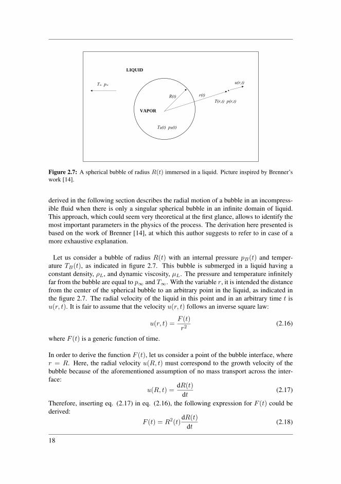
2.7 A spherical bubble of radius R(t) immersed in a liquid. Picture inspiredby Brenner’s work [14]. . . . . . . . . . . . . . . . . . . . . . . . . . . . 18

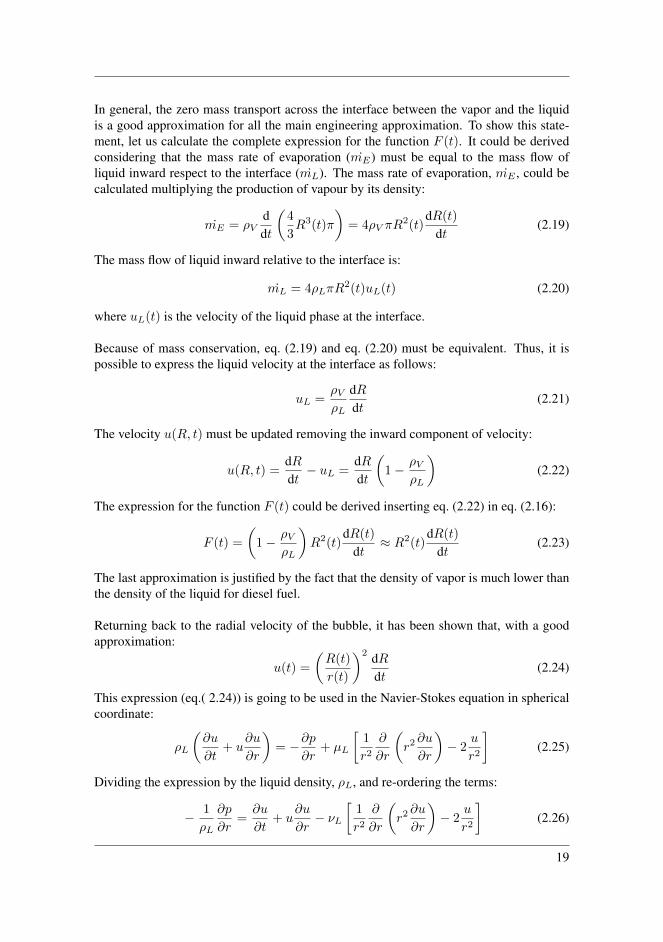
2.8 The forces per unit of area acting on a portion of the interface. Pictureinspired by Brenner’s work [14]. . . . . . . . . . . . . . . . . . . . . . . 20

2.9 Scheme of the fuel injection system of a two-stroke diesel engine. Pictureprovided by MAN Energy Solutions . . . . . . . . . . . . . . . . . . . . 21

2.10 Scheme of the FIVA valve. Picture from [1] . . . . . . . . . . . . . . . . 22

xv

3.1 The two overlapping meshes and the relation between the acceptors, donorsand active cells. Picture from the Userguide [45] . . . . . . . . . . . . . . 33

4.1 Streamlines (above) and the pressure distribution (below) along the lengthof a one dimensional converging-diverging nozzle. The dotted line showsthe onset of the multiphase flow. In case of cavitation, it is not possible todescribe the pressure distribution far from the throat. The picture is fromHogendoorn’s Master thesis [26]. . . . . . . . . . . . . . . . . . . . . . . 37

4.2 Scheme of the break-off cycle in a converging-diverging nozzle. The flowis from left to right. . . . . . . . . . . . . . . . . . . . . . . . . . . . . . 39

4.3 Overview of the experimental rig described in the experiment by Jahanguiret al. [28] and reported in Hogendoorn’s Master thesis [26]. . . . . . . . . 41

4.4 The geometry of the converging-diverging nozzle used in the simulations. 414.5 Picture of the mesh, with the two rectangular area refinement. . . . . . . . 424.6 The function f(ρ) for n = 10. . . . . . . . . . . . . . . . . . . . . . . . 454.7 The four edges in the Venturi nozzles: inlet, outlet, symmetry and wall. . 454.8 The line probes used to investigate the pressure distribution in the converging-

diverging nozzle. . . . . . . . . . . . . . . . . . . . . . . . . . . . . . . 474.9 Pressure distribution in the converging-diverging nozzle when the cavita-

tion model has not been enabled. This fact justifies the negative pressuredetected at the throat by the line probe 2-2. . . . . . . . . . . . . . . . . 47

4.10 The velocity vector field (integral convolution) when the cavitation modelis disabled. . . . . . . . . . . . . . . . . . . . . . . . . . . . . . . . . . 48

4.11 Time evolution of the volume fraction of vapor detected by a point probelocated in the neck of the Venturi nozzle (above) and the spectral analysis(below). The test is conducted using the standard k-ε turbulence model. . 49

4.12 The volume fraction of vapor field when the standard k-ε turbulence modelis used. No detachment is observed. . . . . . . . . . . . . . . . . . . . . 49

4.13 Time evolution of the volume fraction of vapor detected by a Point probelocated in the neck of the Venturi nozzle (above) and the spectral anal-ysis (below). The test is conducted using the k-ε turbulence model withReboud’s correction. . . . . . . . . . . . . . . . . . . . . . . . . . . . . 50

4.14 The re-entrant jet and the detachment of the vapor sheet. Results obtainedthrough the implementation of the Reboud’s correction in k-ε turbulencemodel. . . . . . . . . . . . . . . . . . . . . . . . . . . . . . . . . . . . . 50

4.15 Time evolution of the volume fraction of vapor detected by a point probelocated in the neck of the Venturi nozzle (above) and the spectral analysis(below). The test is conducted using the k-ω turbulence model with theReboud’s correction. . . . . . . . . . . . . . . . . . . . . . . . . . . . . 51

4.16 Time evolution of the volume fraction of vapor detected by a Point probelocated in the neck of the Venturi nozzle (above) and the spectral analysisof the signal (below). The test is conducted using the k-ω turbulent modelwith Reboud’s correction and full Rayleigh-Plesset cavitation model. . . . 51

4.17 Detachment of the vapor bubble with the Rayleigh-Plesset cavitation model,Reboud’s correction and k − ε turbulence model. . . . . . . . . . . . . . 51

xvi

4.18 The break off cycle obtained using the SST k − ω turbulence model withthe Reboud’s correction . . . . . . . . . . . . . . . . . . . . . . . . . . . 53

4.19 Representation of the re-entrant jet detected in the velocity field at the nondimensional time 0.24. The simulation uses the k-ω turbulence model withthe Reboud’s correction. . . . . . . . . . . . . . . . . . . . . . . . . . . 54

4.20 Mesh independence study; the four meshes have the following number ofcells: 31070, 36175, 51538, 104847. . . . . . . . . . . . . . . . . . . . . 55

4.21 The spindle guide, the original geometry provided by MAN Energy Solu-tions. . . . . . . . . . . . . . . . . . . . . . . . . . . . . . . . . . . . . . 58

4.22 The spindle, the original geometry provided by MAN Energy Solutions. . 584.23 The fuel nozzle, the original geometry provided by MAN Energy Solu-

tions. The nozzle holes are indicated with H1, H2, H3, H4 from right toleft. . . . . . . . . . . . . . . . . . . . . . . . . . . . . . . . . . . . . . 58

4.24 The original geometry of the assembly (Left) and its modified version(Right). . . . . . . . . . . . . . . . . . . . . . . . . . . . . . . . . . . . 59

4.25 The geometry of the injector with expansion volumes (in orange). In thispicture, the cut-off shaft is at full lift. . . . . . . . . . . . . . . . . . . . . 60

4.26 The polyhedral and the trimmer mesh, in red the overset, in blue the back-ground when the fuel valve is full open. On the right the trimmer meshafter the initialization. . . . . . . . . . . . . . . . . . . . . . . . . . . . . 62

4.27 The spindle and a section of the background (in blue) and overset mesh (ingray) . . . . . . . . . . . . . . . . . . . . . . . . . . . . . . . . . . . . . 62

4.28 The displacement of the cut of shaft for the opening (Left) and closing(Right) . . . . . . . . . . . . . . . . . . . . . . . . . . . . . . . . . . . . 63

4.29 The inlet and outlet pressure at the SOI (Left) and EOI (Right) . . . . . . 644.30 The mass flow per each of the nozzle holes; results from the polyhedral

mesh. . . . . . . . . . . . . . . . . . . . . . . . . . . . . . . . . . . . . 664.31 The mass flow per each of the nozzle hole; results from the trimmer mesh

with alignment. . . . . . . . . . . . . . . . . . . . . . . . . . . . . . . . 664.32 Total mass flow for the two meshes (in blue and green) and the reference

values from 1D-Hydcode (in black). . . . . . . . . . . . . . . . . . . . . 664.33 Pressure recorded by the Point probe located in the sac; evolution of the

signal in time and in the frequency domain. The first peak in the spectralanalysis is due to the increase of the pressure in the boundary, while it isbelieved that the second peak is due to the pressure fluctuations inducedby the pressure wave. . . . . . . . . . . . . . . . . . . . . . . . . . . . . 67

4.34 The momentum flow per each of the nozzle hole; results from the polyhe-dral mesh. . . . . . . . . . . . . . . . . . . . . . . . . . . . . . . . . . . 68

4.35 The momentum flow per each of the nozzle hole; results from the trimmermesh. . . . . . . . . . . . . . . . . . . . . . . . . . . . . . . . . . . . . 68

4.36 Velocity field (integral convolution) in a section of hole H1 at the openingof the fuel valve. . . . . . . . . . . . . . . . . . . . . . . . . . . . . . . 69

4.37 Pressure field in a section of hole H1 at the opening of the fuel valve. . . . 704.38 Velocity field (integral convolution) in a section of hole H2 at the opening

of the fuel valve . . . . . . . . . . . . . . . . . . . . . . . . . . . . . . . 71

xvii

4.39 Pressure field in a section of hole H2 at the opening of the fuel valve. . . . 724.40 Velocity field (integral convolution) in a section of hole H3 at the opening

of the fuel valve. . . . . . . . . . . . . . . . . . . . . . . . . . . . . . . 734.41 Pressure field in a section of hole H3 at the opening of the fuel valve. . . . 744.42 Velocity field (integral convolution) in a section of hole H4 at the opening

of the fuel valve. . . . . . . . . . . . . . . . . . . . . . . . . . . . . . . 754.43 Pressure field in a section of hole H4 at the opening of the fuel valve. It is

interesting to note a large vortex which is generated at the entrance of thenozzle hole. . . . . . . . . . . . . . . . . . . . . . . . . . . . . . . . . . 76

4.44 Streamlines at the end of the opening event (t = 1.8 ms) . . . . . . . . . 774.45 The mass flow per each of the nozzle hole; results from the polyhedral mesh. 784.46 The mass flow per each of the nozzle hole; results from the trimmer mesh. 784.47 Total mass flow for the two meshes (in blue and green) and reference val-

ues from 1D-Hydcode. . . . . . . . . . . . . . . . . . . . . . . . . . . . 794.48 The error between the mass flow from the CFD simulations and 1D-Hydcode. 804.49 Pressure recorded in the sac volume by the point probe. . . . . . . . . . . 814.50 The vortex core location depicted through iso-surface of the pressure field. 81

5.1 A glimpse on cavitation phenomenon; percentage of volume of fraction ofvapor; 1% in light blue, 5% in magenta, 10% in dark blue. . . . . . . . . 87

5.2 Bottom view, iso-surface 25% of volume fraction of vapor and streamlines.A swirling flow might be clearly detected. . . . . . . . . . . . . . . . . . 88

5.3 Volume fraction of vapour in four cylindrical section of the nozzle hole.The reference radii of the cylindrical surfaces coaxial with the injector are3.5 mm, 4.5 mm, 5.5 mm, 6.5 mm. . . . . . . . . . . . . . . . . . . . . . 89

5.4 The velocity field (integral convolution) of the nozzle holes when the valveis 55% open . . . . . . . . . . . . . . . . . . . . . . . . . . . . . . . . . 90

5.5 The pressure field of the nozzle holes when the valve is 55% open. Notethe vortex structure in the nozzle hole 4, which causes the growth of thevapor string. . . . . . . . . . . . . . . . . . . . . . . . . . . . . . . . . . 90

5.6 A glimpse on the cavitation phenomenon, percentage of volume of fractionof vapor; 1% in light blue, 5% in magenta, 10% in dark blue. . . . . . . . 91

5.7 Bottom view, isosurface 5% of volume fraction of vapor and streamlines. 925.8 Iso-surface (10% of the volume fraction of vapor) and streamlines when

the valve is 75% open . . . . . . . . . . . . . . . . . . . . . . . . . . . . 935.9 The velocity field (integral convolution) of the nozzle holes when the valve

is 75% open . . . . . . . . . . . . . . . . . . . . . . . . . . . . . . . . . 945.10 The pressure field of the nozzle holes when the valve is 75% open . . . . 945.11 Discharge coefficient through the nozzle holes and reference data from

MAN Energy Solutions. . . . . . . . . . . . . . . . . . . . . . . . . . . 965.13 A glimpse on the cavitation phenomenon when the fuel valve is at full lift.

The cells with the volume fraction of vapor larger than a threshold havebeen highlighted; 1% in light blue, 5% in magenta, 10% in dark blue. . . 97

5.12 Pressure distribution along the symmetry axis and the inferior wall of thefour nozzle holes . . . . . . . . . . . . . . . . . . . . . . . . . . . . . . 98

5.14 Bottom view, iso-surface 5% of volume fraction of vapor and streamlines. 98

xviii

5.15 The velocity field (integral convolution) of the nozzle holes when the valveis 100% open . . . . . . . . . . . . . . . . . . . . . . . . . . . . . . . . 99

5.16 The pressure field of the nozzle holes when the valve is 100% open. Thereader could note the vortex core in the sac in the picture of the nozzle H2. 99

5.17 Mass flow through the four orifices and total mass flow versus time. . . . 1005.18 Momentum flow through the four orifices versus time. . . . . . . . . . . . 1015.19 Velocity field in the seat in the first instant of the SOI. . . . . . . . . . . . 1015.20 Pressure and volume fraction of vapor scalar fields. . . . . . . . . . . . . 1025.21 Percentage of the volume of the nozzle hole occupied by fuel vapor with

respect to time. . . . . . . . . . . . . . . . . . . . . . . . . . . . . . . . 1025.22 Phase mass flow through the four orifices versus time. . . . . . . . . . . . 1035.23 10% volume fraction of vapor isosurface. Visualization of the cavitation

regime in the first peak of figure 5.21. . . . . . . . . . . . . . . . . . . . 105

6.1 Pressure recorded by a point probe in the inlet of the injector. . . . . . . . 1186.2 Pressure fluctuations at the inlet of the injector. . . . . . . . . . . . . . . 1186.3 Analysis of the pressure signal in the frequency domain. . . . . . . . . . 1196.4 Momentum flow, end of injection. Results form the trimmer mesh. . . . . 119

xix

xx

Nomenclature

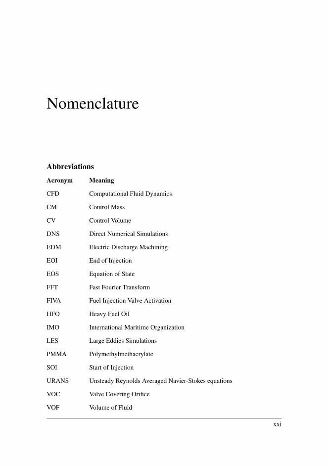
Abbreviations

Acronym Meaning

CFD Computational Fluid Dynamics

CM Control Mass

CV Control Volume

DNS Direct Numerical Simulations

EDM Electric Discharge Machining

EOI End of Injection

EOS Equation of State

FFT Fast Fourier Transform

FIVA Fuel Injection Valve Activation

HFO Heavy Fuel Oil

IMO International Maritime Organization

LES Large Eddies Simulations

PMMA Polymethylmethacrylate

SOI Start of Injection

URANS Unsteady Reynolds Averaged Navier-Stokes equations

VOC Valve Covering Orifice

VOF Volume of Fluid

xxi

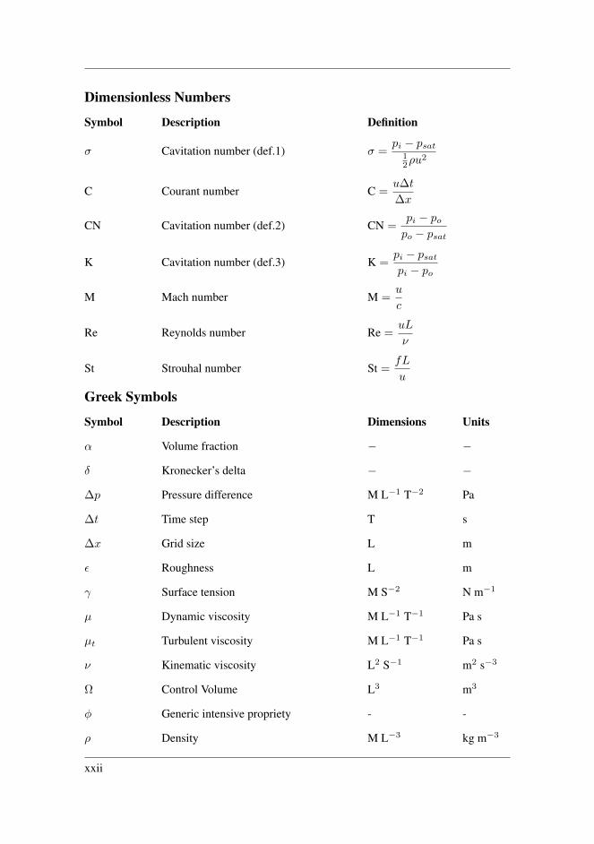
Dimensionless Numbers

Symbol Description Definition

σ Cavitation number (def.1) σ =pi − psat

12ρu

2

C Courant number C =u∆t

∆x

CN Cavitation number (def.2) CN =pi − popo − psat

K Cavitation number (def.3) K =pi − psatpi − po

M Mach number M =u

c

Re Reynolds number Re =uL

ν

St Strouhal number St =fL

u

Greek Symbols

Symbol Description Dimensions Units

α Volume fraction − −

δ Kronecker’s delta − −

∆p Pressure difference M L−1 T−2 Pa

∆t Time step T s

∆x Grid size L m

ε Roughness L m

γ Surface tension M S−2 N m−1

µ Dynamic viscosity M L−1 T−1 Pa s

µt Turbulent viscosity M L−1 T−1 Pa s

ν Kinematic viscosity L2 S−1 m2 s−3

Ω Control Volume L3 m3

φ Generic intensive propriety - -

ρ Density M L−3 kg m−3

xxii

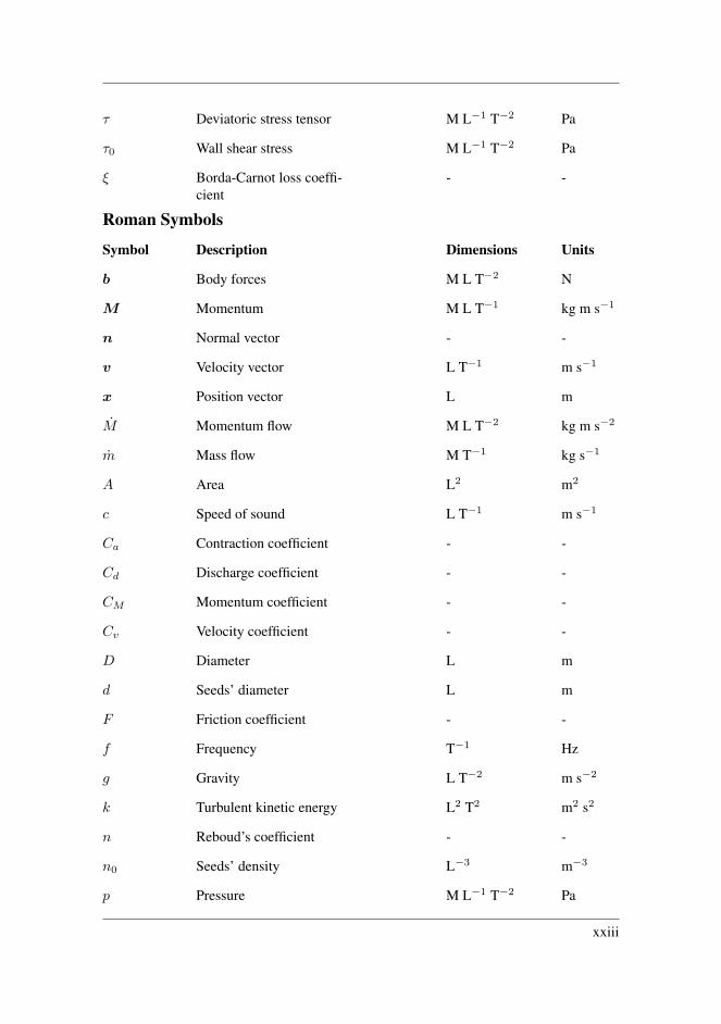
τ Deviatoric stress tensor M L−1 T−2 Pa

τ0 Wall shear stress M L−1 T−2 Pa

ξ Borda-Carnot loss coeffi-cient

- -

Roman Symbols

Symbol Description Dimensions Units

b Body forces M L T−2 N

M Momentum M L T−1 kg m s−1

n Normal vector - -

v Velocity vector L T−1 m s−1

x Position vector L m

M Momentum flow M L T−2 kg m s−2

m Mass flow M T−1 kg s−1

A Area L2 m2

c Speed of sound L T−1 m s−1

Ca Contraction coefficient - -

Cd Discharge coefficient - -

CM Momentum coefficient - -

Cv Velocity coefficient - -

D Diameter L m

d Seeds’ diameter L m

F Friction coefficient - -

f Frequency T−1 Hz

g Gravity L T−2 m s−2

k Turbulent kinetic energy L2 T2 m2 s2

n Reboud’s coefficient - -

n0 Seeds’ density L−3 m−3

p Pressure M L−1 T−2 Pa

xxiii

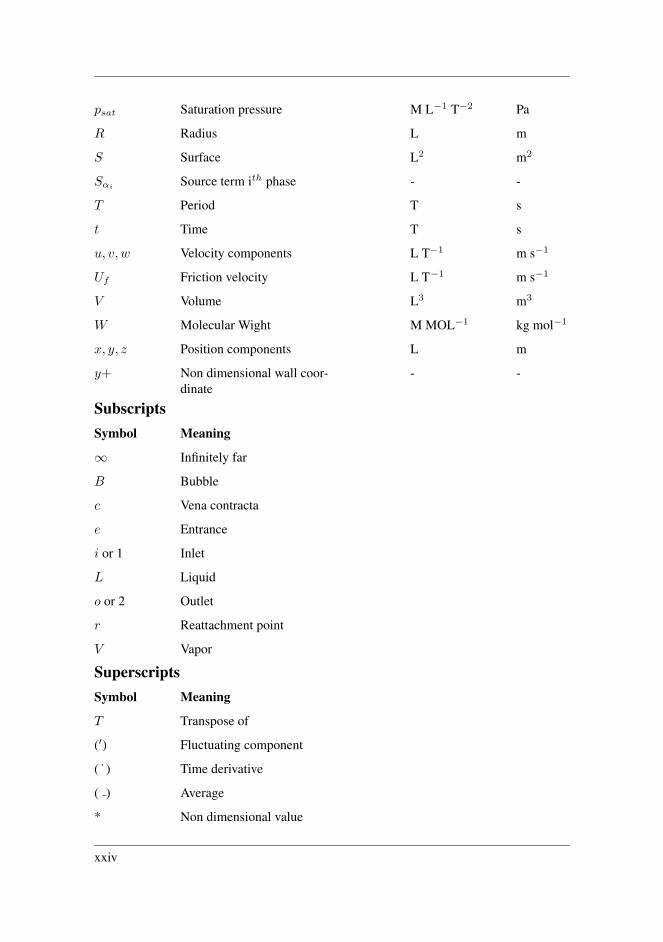
psat Saturation pressure M L−1 T−2 Pa

R Radius L m

S Surface L2 m2

SαiSource term ith phase - -

T Period T s

t Time T s

u, v, w Velocity components L T−1 m s−1

Uf Friction velocity L T−1 m s−1

V Volume L3 m3

W Molecular Wight M MOL−1 kg mol−1

x, y, z Position components L m

y+ Non dimensional wall coor-dinate

- -

SubscriptsSymbol Meaning

∞ Infinitely far

B Bubble

c Vena contracta

e Entrance

i or 1 Inlet

L Liquid

o or 2 Outlet

r Reattachment point

V Vapor

SuperscriptsSymbol Meaning

T Transpose of

(′) Fluctuating component

( ˙ ) Time derivative

( ) Average

* Non dimensional value

xxiv

Chapter 1Introduction

In the last fifty years, the growth of environmental awareness has led to public demandfor environmental safeguards and remedies to air pollution. Under these circumstances,standards for the harmful exhaust produced by diesel engines were established and theregulations forced the manufactures to invest on research and development of new tech-nologies. In common imaginary, diesel engine innovation is closely linked to the automo-tive industry; since the late seventies, more than 20 thousands patents have been registeredin this sector [13]. Even today, although diesel engines have been called into question afterthe recent emission scandals, the major car firms are still pledging to invest billions on itsdevelopment.

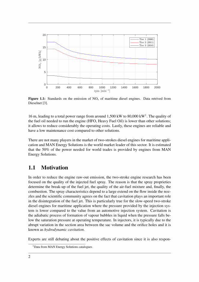
The maritime engineering industry has been affected by these standards more recently.The first international regulation on pollution due to merchant ships was ratified in 1997by the International Maritime Organization (IMO) in the convention denominated MAR-POL 73/78; the Annex VI, named Prevention of Air Pollutants for Ships came into force inMay 2005. Year after year, the standards are continuously revised by limiting the amountof nitrogen oxides, sulphurs, hydrocarbons and soot. An overview of the evolution of thestandards in terms of NOx limits (similar plots could be obtained also for other exhausts)is presented in figure 1.1. The tightening of emission controls is evident from the analysisof the picture; in this regard, the percentage of the emission of NOx has dropped of around80% in the last 20 years and it will inevitably decrease further in future.

In this work, the focus is on slow-speed two-stroke diesel engines. This propulsion systemis the most popular among the large freight ships; there are many different reasons for that.First of all, the two-stroke engine has as an higher power to weight ratio in comparisonwith the four stroke engine. In fact, there is a direct coupling between the crankshaft andthe propeller, avoiding the need of reductor and gear shift. This solution is possible be-cause of the low number of right per minute, on average, around 100 rpm. Higher regimesare not possible due to the high inertia of the moving parts. Just to mention only a fewtypical dimensions, the bore is from 30 to 95 cm, the height of the engine is from 5.9 m to

1

0 200 400 600 800 1000 1200 1400 1600 1800 2000

0

5

10

15

20

Figure 1.1: Standards on the emission of NOx of maritime diesel engines. Data retrived fromDieselnet [3].

16 m, leading to a total power range from around 1,500 kW to 80,000 kW1. The quality ofthe fuel oil needed to run the engine (HFO, Heavy Fuel Oil) is lower than other solutions;it allows to reduce considerably the operating costs. Lastly, these engines are reliable andhave a low maintenance cost compared to other solutions.

There are not many players in the market of two-strokes diesel engines for maritime appli-cation and MAN Energy Solutions is the world market leader of this sector. It is estimatedthat the 50% of the power needed for world trades is provided by engines from MANEnergy Solutions.

1.1 MotivationIn order to reduce the engine raw-out emission, the two-stroke engine research has beenfocused on the quality of the injected fuel spray. The reason is that the spray proprietiesdetermine the break-up of the fuel jet, the quality of the air-fuel mixture and, finally, thecombustion. The spray characteristics depend to a large extend on the flow inside the noz-zles and the scientific community agrees on the fact that cavitation plays an important rolein the disintegration of the fuel jet. This is particularly true for the slow-speed two-strokediesel engines for maritime application where the pressure provided by the injection sys-tem is lower compared to the value from an automotive injection system. Cavitation isthe adiabatic process of formation of vapour bubbles in liquid when the pressure falls be-low the saturation pressure at operating temperature. In injectors, it is typically due to theabrupt variation in the section area between the sac volume and the orifice holes and it isknown as hydrodynamic cavitation.

Experts are still debating about the positive effects of cavitation since it is also respon-

1Data from MAN Energy Solutions catalogues

2

sible of enhancing mechanical wear as consequence of bubbles collapse and a lot of effortis being put on characterizing the phenomenon. Unfortunately, the experimental studyof cavitation in the context of diesel injector is very complex to perform. In fact, thedimensions of the nozzle are in the millimeter range and the pressure difference is tremen-dously high. The visualization of the the vapour bubbles is only possible with the use oftransparent nozzle made in acrylic (for instance in Polymethylmethacrylate, PMMA) butthe pressures must be scaled to avoid the mechanical failure. In these experiments, eventhough the cavitation number, a non-dimensional parameter that describes the cavitationregime, identically replicates the operating condition, the Reynolds number could signifi-cantly differ from it. Moreover, the experimental investigation under transient conditionsis even more challenging due to the short duration of the injection event. The study of tran-sients (the opening and the closing of the fuel valve) is of importance since multiple andshort duration injections are often used to cope with the emission targets. Indeed, in caseof pilot injection, the transients are the dominant part of the entire process. Under thesecircumstances, the computational fluid dynamics (CFD) is a fundamental tool to predictthe results and improve the injector design.

This project intends to investigate the cavitation in transient condition in two-stroke dieselengine injector by means of a commercial computational fluid dynamics software, STARCCM+. Before going into details on the methods and results, the state of the art withinthis topic is briefly reported in the following section.

1.2 State of Art

In this section, the most relevant developments in the technology and design of direct injec-tion system are introduced. In the last fifty years, a massive research has been conductedby the industry and the academia to characterize the flow inside the nozzle holes and inthe first millimeters of the spray region. These studies led to some important achievementssuch as the introduction of a sliding fuel valve, allowing to cope with the emission regu-lations. Most of the researches were conducted with full lift valve, neglecting the motionof the needle; the underlying assumption was that the transients had a weak effect on theinjection cycle, being only a small fraction of the entire injection cycle. This hypothesis isno more valid when pre-injections or post-injections are considered, since injectors workmost of the time with partial lift and the event is extremely short. At the moment, mostof the recent works are aimed at answering questions such as: what is the relationship be-tween the needle lift and the in-nozzle flow and jet development? And between the needlelift and discharge and momentum coefficient? Despite the answers strictly depend on thegeometry of the injectors, engineers and scientists are trying to demonstrate some commonfeatures and the main results are here presented.

1.2.1 Classification and design of injectors

Before starting with the description of the most popular classification of direct injectors,it is worthwhile to clarify the terminology in order to avoid misunderstandings. At this

3

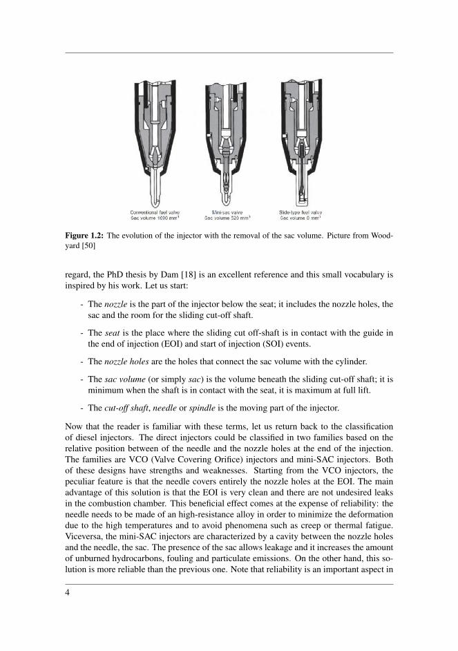
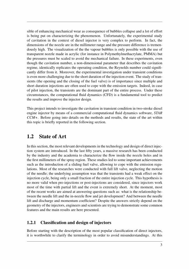
Figure 1.2: The evolution of the injector with the removal of the sac volume. Picture from Wood-yard [50]

regard, the PhD thesis by Dam [18] is an excellent reference and this small vocabulary isinspired by his work. Let us start:

- The nozzle is the part of the injector below the seat; it includes the nozzle holes, thesac and the room for the sliding cut-off shaft.

- The seat is the place where the sliding cut off-shaft is in contact with the guide inthe end of injection (EOI) and start of injection (SOI) events.

- The nozzle holes are the holes that connect the sac volume with the cylinder.

- The sac volume (or simply sac) is the volume beneath the sliding cut-off shaft; it isminimum when the shaft is in contact with the seat, it is maximum at full lift.

- The cut-off shaft, needle or spindle is the moving part of the injector.

Now that the reader is familiar with these terms, let us return back to the classificationof diesel injectors. The direct injectors could be classified in two families based on therelative position between of the needle and the nozzle holes at the end of the injection.The families are VCO (Valve Covering Orifice) injectors and mini-SAC injectors. Bothof these designs have strengths and weaknesses. Starting from the VCO injectors, thepeculiar feature is that the needle covers entirely the nozzle holes at the EOI. The mainadvantage of this solution is that the EOI is very clean and there are not undesired leaksin the combustion chamber. This beneficial effect comes at the expense of reliability: theneedle needs to be made of an high-resistance alloy in order to minimize the deformationdue to the high temperatures and to avoid phenomena such as creep or thermal fatigue.Viceversa, the mini-SAC injectors are characterized by a cavity between the nozzle holesand the needle, the sac. The presence of the sac allows leakage and it increases the amountof unburned hydrocarbons, fouling and particulate emissions. On the other hand, this so-lution is more reliable than the previous one. Note that reliability is an important aspect in

4

Figure 1.3: Nozzle hole with the most important geometrical dimensions: the inlet and outlet diam-eter (Di and Do), the length L and entrance radius re. Picture from Martı Gomez-Aldaravı [34]

engineering, but it is crucial in the marine sector, being the navigation of the large cargoships in open ocean.

In the early 2000s, the research engineers of MAN Energy Solutions (at the time MANDiesel & Turbo) redesigned the fuel injection valve in order to have both the advantagesof the VOC and mini-SAC injectors. The improved design consists in a sliding valvethat eliminates completely the sac volume and reduces the consequent waste of oil. It de-creases the emissions and, at the same time, assures great reliability. Of course, because ofthe clearance between the inner surface of the nozzle and the other surface of the cut-offshaft and the high pressure difference between the two rooms, leakage will occur but it isminimized. Because of its large beneficial effects, this type of valve has become the stan-dard in the engines designed and produced by MAN Energy Solutions. A representationof the mini-SAC fuel valve and the slide fuel valve is depicted in figure 1.2.

With regards to cavitation, the scientific community has studied the impact of shape ofthe nozzle hole on the nucleation and growth of vapor pockets. The main reference of thisparagraph is the PhD thesis by Martı Gomez-Aldaravı [34], where the most relevant resultsare summarized. Refer to figure 1.3 for the most significant geometrical dimensions. Theratios of the parameters plotted in figure 1.3 give indications on the onset of cavitation.Let us start considering the ratio between the entrance radius re and the inlet diameter Di.When re/Di is large enough (Martı Gomez-Aldaravı reported the value 0.2), the pressurelosses due to the sudden contraction (Borda-Carnot losses) could be neglected. As a con-sequence of that, it is unlikely that the pressure drops under the saturation limit. In otherwords, high values of re/Di allow to avoid cavitation.The ratio between the inlet and outlet diameter, Di/Do, is extremely relevant too; when itis larger than 1 the shape of the nozzle holes is convergent; when it is equal to 1 it is cylin-drical, otherwise it is divergent. In the literature, it is popular to introduce a new variable,namely the k-factor:

k-factor =Di −Do

10µm(1.1)

A positive k-factor (or alternatively when the ratio Di/Do is larger than 1) is favorable tosuppress cavitation.

5

Lastly, the other characteristic ratio is L/Do, where L is the length of the nozzle. Anhigh value of L/Do reduces the possibility of cavitation since the pressure losses due tothe friction are larger. This means that, assuming that the pressure at the boundaries isconstant, the pressure in the critical section is larger for a high value of the ratio L/Do,and, ideally, above the saturation limit. Moreover, in this solution, the discharge coefficientis maximized because the location of detachment is far from the exit.

1.2.2 The Unsteady Cavitation in LiteratureCavitation in diesel engines injectors under stationary conditions has been widely inves-tigated by the scientific community from 1959 when Bergwerk [10] published the firstarticle related to this topic. Since then, scientists and engineers have focused both on ex-perimental studies and numerical modeling of the in-nozzle flow and fuel spray pattern.The experiments are aimed at showing the effects of cavitation in terms of jet proprietiessuch as spray cone angle, penetration length or Sauter Mean Diameter (SMD). Because ofthe costs and limitations of setting up an experimental cavitation rig and the increase ofcomputing power, the flow modelling through CFD software has become more and morepopular in the industry and academia even though experiments are still needed to validatethe codes. The technical literature on in-nozzle cavitation is very comprehensive, espe-cially regarding the cavitation at full lift valve or at partial lift valve but always in steadycondition. The reason is that the attention of the scientific community is addressed to themain injection because it is the predominant event; in fact, the transients have only a shortduration. Because of the use of the pilot injection to cope with the emission limits, thetransients are getting more and more relevant in these days, and they have started to be in-vestigated. In the following paragraphs, the most relevant papers on this topic are reportedin order to give the reader an overview about the main results that were achieved. Beingthe slide valve used mainly in the marine engineering, most of the authors referred to VCOand mini-SAC injectors, because they are used in the automotive sector. Despite of that, itis believed that the some of the results might be applied also for the injector of this project.

Among the first experimental works which take into account the transients, there is thestudy by Badock et al. [7]. The authors used both shadowgraph and laser sheet techniquesto visualize cavitation inside a mini-SAC injector made of perspex with a cylindrical noz-zle. Badock et al. observed the presence of large bubbles of gas in the sac hole at the startof the injection as a consequence of the ingestion of air at the end of injection of the previ-ous cycle. This phenomenon was later shown using x-ray phase contrast by the ArgonneNational Laboratory; a nice visualization might be found in [2]. When the pressure dif-ference of the common rail and discharge chamber is around 240 bar, Badock et al. noteda film of vapor around the walls of the nozzle holes (situation known as super-cavitationregime). The authors measured the time required to the development of the vapor film andthey found that it is equal to 0.1 ms for their geometry. Moreover they noted that increas-ing the pressure at the inlet does not produce any significant effects on the cavitation filmand they concluded that the effective area of the liquid jet is almost independent of theinjection pressure when the super-cavitation is reached. Nevertheless, a liquid core wasobserved in all the experimental conditions.

6

Neroorkar et al. [37] simulated the transient needle effects in a tapered five holes mini-SACinjector. In order to simulate the motion, the authors used a method consisting in addingor removing cell layers when the cells around the needle are stretched or compressed morethan an user-specified value. Unfortunately, their method requires a minimum lift; in otherwords, the needle and the seat never get in contact and a leak of fuel always occurs. Forlarge duration of the injection and large amplitude of the needle motion, their simulationsestablished a satisfactory agreement with the experimental data. Neroorkar et al. demon-strated the presence of swirling flow which affects the amount of fuel mass discharged inthe cylinder. In particular, this swirling flow has a higher intensity for small needle lifts.The authors tested the code for small duration injection events too but, due to the assump-tion of the minimum lift, their results showed large discrepancies from the experiments.

Blessing and al. [12] studied the flow in a mini-SAC injector at different needle lift. Theyused a not scale close-to-reality geometry for validation and a real multi-holes mini-SACinjector; their investigation is mainly addressed to the influence of the needle lift on thespray parameters. In particular, for their geometry, the authors related the needle lift withcone spray angle and the penetration length. In addition, they studied the influence of thek-factor on the cavitation onset. They found that a divergent nozzle shows the strongestcavitation tendency. For a cylindrical nozzle, it is reported that the cavitation tendency atthe center of the nozzle hole is increased during the needle opening phase. It is unclearhow the authors performed their experiments and simulation; in fact it is not stated howthe needle is moved in their rig and what numerical method is used in their CFD code. Forthis reason, it seems that they performed the tests in steady state condition.

A recent article which evaluated the influence of the needle lift in diesel injector nozzlesis by Salvador et al. [19]. With the assumption that the actual transient injection processmight be simplified considering the needle at different lift and steady-state, the authorsperformed several simulations using a multi-holes micro-SAC injector and LES turbulentmodel. At small lift, they noted the presence of cavitation pockets close to the needleseat; same results was also obtained by other authors as reported by Baumgartner [8]. Theneedle lift has a large impact on the in-nozzle flow, in terms of vorticity and turbulentstructures within the holes.

Even if it does not deal with transients, the work by Payri et al. [41] is an excellent refer-ence to understand the effect of cavitation on mass discharge, momentum flux and outletvelocity. As other authors, Payri et al. analysed the influence of the nozzle geometry(cylindrical and conical) when the needle is at maximum lift for VCO injector. The mainconclusion from the authors is that cavitation appears only in cylindrical nozzle, due to thefact that the flow acceleration is more gradual in the conical nozzle. In addition, the notedthat, in cavitating condition, the mass flow decreases almost linearly with the square rootof the cavitation number, K. On the contrary, the momentum flux is always proportional tothe pressure difference and the momentum coefficient is independent from the cavitationnumber. The authors showed that the outlet velocity increases in case of cavitation while,in the same conditions, the section area decreases.

7

The experimental investigation by Hult, Simmonk, Matlok and al. [27] is particularly rel-evant to this work. Indeed, it is one of the few papers in literature where the object ofthe study is a slide fuel valve. This typology of injector has recently become the stan-dard for slow-speed two-stokes diesel engines and, more importantly, it is the injector thatwill be analysed in this project. Unfortunately, because of the practical difficulties in as-sessing the transients, the authors put most of their effort on characterizing cavitation instationary condition. In other words, the experiments are conducted at fixed lift and steadyconditions. Shadowgraphy in transparent nozzle made in PMMA is the technique used tovisualize the cavitation pattern and PIV (Particle Image Velocimetry) is used to study thevelocity in the sac and nozzle. The authors showed that cavitation appears to originate atthe edge of the nozzle holes due to the high velocity gradient and at the centre of smallvortex-shape structure. When the cavitation number is severely increased, the cavitationfilled the outlet section entirely. The experiments were reproduced through a CFD numer-ical simulation and the authors found a good agreement between the two dataset in termsof discharges mass flow and velocity distribution.

1.3 The Project and its ObjectiveThe aim of this project is to study the transient in-nozzle flow in two stroke diesel injectors,focusing on the motion of the cut-off shaft and the vapor structures which might occur inthe nozzle holes and seat. The project is conducted in collaboration with MAN EnergySolutions, which provided the geometry of the injector and some data for the validation.

The project followed four major stages:

• Literature review and critical analysis of paper about in-nozzle flow for diesel en-gines.

• Validation of unsteady cavitation. The simulation of the periodic shedding of vaporbubbles in a converging-diverging nozzles is performed and the results are comparedwith the experimental data. This test allows to tune up the cavitation model and gainconfidence with it.

• Validation of the overset mesh, considering the real injector system and one phaseflow. The motion of the needle is implemented in the software, as well as the bound-ary conditions and the diesel proprieties. The results are compared with the datafrom an internal code of MAN Energy Solutions.

• Simulation of the multiphase flow with still and moving needle.

As far as I know, this is the first work aimed at simulating the motion of the fuel valve ina slide valve injection system through the use of the overset mesh technique. At the startof the project, the lack of know-how about the modelling of cavitation and the use of theoverset forced to spend a lot of time in reading the Userguide to understand the effects ofthese method on the governing equations.

8

Chapter 2Theory

This chapter is intended to provide the reader with the basic notions of the in-nozzle flowin diesel injectors. In the first section, after a brief introduction of cavitation theory andcavitation mechanisms which might occur in diesel injectors, the effects of the multiphaseflow in the break-up of the fuel jet are discussed. The presence of vapor cavities withinthe nozzle of diesel injectors have both beneficial and adverse consequences which areexplored in the paragraph. The next section is aimed at introducing the milestone of allthe theoretical studies of in-nozzle flow: the one dimensional theory by Nurick [39]. Itexplains why cavitation occurs in diesel injectors and its influence on the mass and mo-mentum flux at the outlet section. These two parameters are well describe by as manycoefficients, the discharge and momentum coefficients. The application of Nurick’s theorywill lead to the definition of one of the most important parameter for cavitating flow: thecavitation number. With the aim of predicting the amount of fuel mass introduced in thecylinder at every injection cycle, the scientific community has put a large effort in relat-ing the discharge coefficient with the Reynolds number and the cavitation number. Someof the main results are provided in this chapter through empirical equations and charts.Finally, the description of the entire injection system of this project is presented.

2.1 Cavitation: Definition and Application in Diesel En-gines

Cavitation is the phenomenon of nucleation of vapour bubbles in liquid when the pressurefalls below the saturation limit at the operating temperature. In this condition, the for-mation of vapor bubbles from pre-existing nucleii (generally impurities) is energeticallyfavourable; the vapor pockets grow, interact with each others and, at the end, collapse.

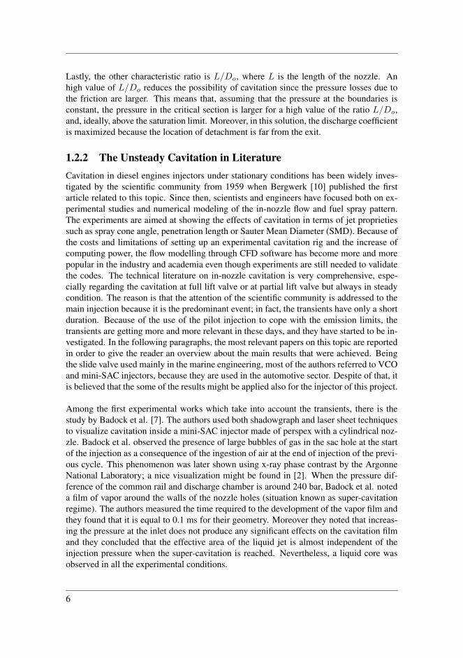
At the first glance, cavitation might seem very similar to boiling: indeed, they both leadto the same phase change, from liquid to vapor. In reality, the physics behind the twoprocesses is completely different. Consider the thermodynamic process paths depicted in

9

Figure 2.1: The thermodynamic process paths for boiling and cavitation in a pressure-temperatureplane. Picture from Hogendoorn [26].

the pressure-temperature plane in figure 2.1. Starting from a generic point of the plane inthe liquid phase, the boiling process is depicted as an horizontal straight line crossing thesaturation liquid/vapor line. The change of phase is at constant pressure; in other words, itis isobaric. On the contrary, cavitation is illustrated as a vertical straight line crossing thesaturation liquid/vapor line, meaning that the phenomenon is isotherm. In real conditions,heat is required for the vaporization but the variation in temperature is negligible for allthe main application, including the case presented in this project1.

In engineering and, in particular, in hydrodynamics, cavitation has been widely studiedbecause of its negative effects on machinery. In fact, the period collapse of the vapour bub-bles generates cyclic stresses on the surface in contact with the liquid. This phenomenonis known as surface fatigue and it is responsible for enhancing mechanical wear. Thisis the reason why volumetric pumps, impeller of centrifugal pumps and water turbinesand propellers are designed and installed in order to avoid cavitation. In other contexts,the cavitation might be desired. Just to mention only few examples, in chemistry it is usedto enhance the mixing of different species and in medicine it is used to crush kidney stones.

It has been known from almost fifty years that in-nozzle cavitation might produce positiveeffects in the primary break-up of the fuel jet during the injection event in diesel engines.According to Baumgartner [8], it is possible because of the energy release of the collaps-ing bubbles. This energy is transmitted to the surrounding fluid, increasing the turbulent

1This assumption is no more valid in when a cryogenic liquid are studied, for instance, in rocket engines

10

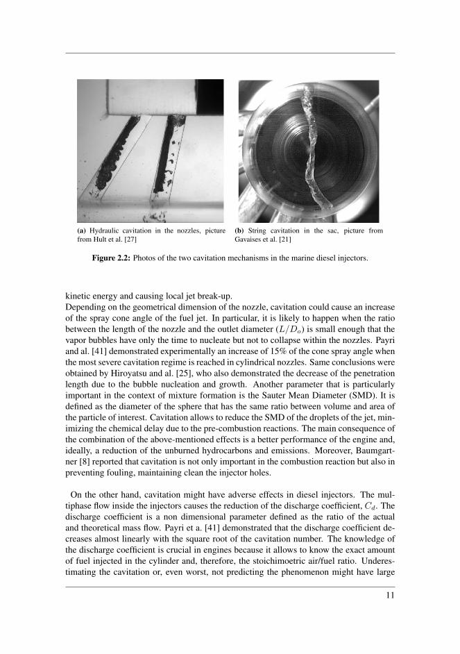
(a) Hydraulic cavitation in the nozzles, picturefrom Hult et al. [27]

(b) String cavitation in the sac, picture fromGavaises et al. [21]

Figure 2.2: Photos of the two cavitation mechanisms in the marine diesel injectors.

kinetic energy and causing local jet break-up.Depending on the geometrical dimension of the nozzle, cavitation could cause an increaseof the spray cone angle of the fuel jet. In particular, it is likely to happen when the ratiobetween the length of the nozzle and the outlet diameter (L/Do) is small enough that thevapor bubbles have only the time to nucleate but not to collapse within the nozzles. Payriand al. [41] demonstrated experimentally an increase of 15% of the cone spray angle whenthe most severe cavitation regime is reached in cylindrical nozzles. Same conclusions wereobtained by Hiroyatsu and al. [25], who also demonstrated the decrease of the penetrationlength due to the bubble nucleation and growth. Another parameter that is particularlyimportant in the context of mixture formation is the Sauter Mean Diameter (SMD). It isdefined as the diameter of the sphere that has the same ratio between volume and area ofthe particle of interest. Cavitation allows to reduce the SMD of the droplets of the jet, min-imizing the chemical delay due to the pre-combustion reactions. The main consequence ofthe combination of the above-mentioned effects is a better performance of the engine and,ideally, a reduction of the unburned hydrocarbons and emissions. Moreover, Baumgart-ner [8] reported that cavitation is not only important in the combustion reaction but also inpreventing fouling, maintaining clean the injector holes.

On the other hand, cavitation might have adverse effects in diesel injectors. The mul-tiphase flow inside the injectors causes the reduction of the discharge coefficient, Cd. Thedischarge coefficient is a non dimensional parameter defined as the ratio of the actualand theoretical mass flow. Payri et a. [41] demonstrated that the discharge coefficient de-creases almost linearly with the square root of the cavitation number. The knowledge ofthe discharge coefficient is crucial in engines because it allows to know the exact amountof fuel injected in the cylinder and, therefore, the stoichimoetric air/fuel ratio. Underes-timating the cavitation or, even worst, not predicting the phenomenon might have large

11

consequences on the performance of the machine. Lastly, cavitation could cause surfacefatigue in the internal walls of the injector, reducing the operative life of the components.

Cavitation takes place in diesel injectors because of two mechanisms. They are namedhydraulic (or sheet) cavitation and vortex (or string) cavitation. The hydraulic cavitationis due to the rapid motion of the fluid from the sac to the nozzle hole as a consequenceof the high pressure difference. Assuming an ideal flow and the conservation of the totalpressure along a streamline, the velocity increment due to the abrupt variation in sectionarea implies a pressure drop. If the pressure falls under the saturation limit, the nucle-ation and growth of the vapor pockets is energetically favourable. The physics behind thesecond mechanism is different; the string cavitation occurs in the center of vortexes as aconsequence of the pressure drops generated by the centrifugal forces. This mechanismhas been discovered recently in diesel marine injectors by Gavaises and al [21]; the authorsfound that the vapor structures might originate from a large vortex located in the sac, asdepicted in figure 2.2.

2.2 Nurick’s One-Dimensional Theory

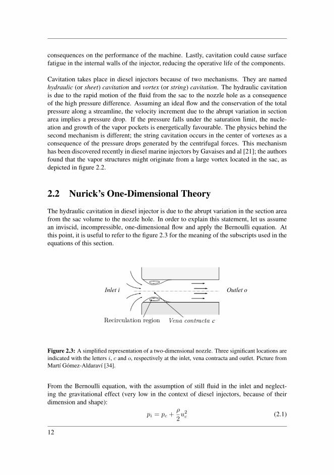
The hydraulic cavitation in diesel injector is due to the abrupt variation in the section areafrom the sac volume to the nozzle hole. In order to explain this statement, let us assumean inviscid, incompressible, one-dimensional flow and apply the Bernoulli equation. Atthis point, it is useful to refer to the figure 2.3 for the meaning of the subscripts used in theequations of this section.

Inlet i Outlet o

c

Figure 2.3: A simplified representation of a two-dimensional nozzle. Three significant locations areindicated with the letters i, c and o, respectively at the inlet, vena contracta and outlet. Picture fromMartı Gomez-Aldaravı [34].

From the Bernoulli equation, with the assumption of still fluid in the inlet and neglect-ing the gravitational effect (very low in the context of diesel injectors, because of theirdimension and shape):

pi = pc +ρ

2u2c (2.1)

12

Recalling the incompressability assumption, from continuity:

ucAc = uiAi (2.2)

It is useful to define some non-dimensional parameters. The first one is the contractioncoefficient Ca. It is defined as the ratio between the effective section area and the actualsection area. When it is evaluated in the point c of the picture 2.3 (vena contracta) and thenozzle is cylindrical:

Ca =Effective areaActual area

=AcAo

=AcAi

(2.3)

The second parameter is the velocity coefficient, Cv . It is equal to the ratio between theeffective velocity and the theoretical velocity at the outlet. It accounts the losses due tothe friction, turbulence and the sudden variation in section area (Borda-Carnot losses). Insymbols:

Cv =Effective velocity

Theoretical velocity=

uo√2(pi−po)

ρ

(2.4)

The last coefficient could be calculated from the previous two and it is named dischargecoefficient, Cd. The discharge coefficient is equal to the ratio between the effective andtheoretical mass flow. When the contraction coefficient (Ca) is referred to the outlet sec-tion, it is equal to:

Cd =Actual mass flux

Theoretical mass flux= CvCa (2.5)

Having introduced these parameters, inserting the above mentioned coefficients in theBernoulli equation (2.1), the following relation could be obtained:

pi − pcpi − po

=

(CvCa

)2

(2.6)

The condition for the incipient cavitation is that pc = psat. Updating eq. (2.6):

pi − psatpi − po

=

(CvCa

)2

(2.7)

In literature, the left hand side of the eq. (2.7) is known as cavitation number:

K =pi − psatpi − po

≈ pipi − po

(2.8)

where the last expression in the right hand side of eq. (2.8) is a good approximation whenthe saturation pressure is much less than the inlet and outlet pressure. In the context ofdiesel injectors, this is always true. In fact, the saturation pressure of the diesel fuel hasa magnitude of 1 kPa, while the injection and cylinder pressures have a magnitude of 104

kPa.

In literature, it is possible to meet some other definitions of the cavitation number. Forinstance, the following in eq. (2.9) is very popular:

CN =pi − popo − psat

≈ pi − popo

(2.9)

13

In context different from diesel injectors, for instance when cavitation is studied aroundhydrofoils or other geometries, the formulation in eq. (2.10) is used:

σ =pi − psat

12ρu

2c

(2.10)

In this work, it will be explicitly stated which definition is used (K, CN or σ) when thecavitation number is mentioned.

2.3 Cavitation RegimesRegardless of the definition of cavitation number which might be used, this non dimen-sional parameter is fundamental to predict amount of vapor due to the hydrodynamic cav-itation. In literature, two regimes are of importance: they are named onset of cavitationand supercavitation.

At this point, it is useful to refer to the article by von Kuensberg Sanne [48] to show thedifferent situations which might be present in the one dimensional nozzle hole of a dieselinjector. The picture 2.4, which is inspired by von Kuensberg Sannes’s work, presents foursituations: a simple turbulent flow (a), the onset of cavitation (b), supercavitation (c) andhydraulic flip (d). The focus is addressed to the pressure distribution along the length ofthe nozzle.

Let us start describing the first case, the simple turbulent flow. In this situation, the separa-tion of the boundary layer occurs due to the abrupt variation in the section area. Since thestreamlines can not follow the sharp angle of the nozzle inlet, the diameter of the streamreaches its minimum, meaning that a vena contracta forms. From the figure 2.4 (a), it ispossible to observe that the flow reattaches in r (rettachment point) and, from this point,the boundary layer starts developing again. At the exit, the flow is not fully developedsince at least 10 diameters [16] (some authors use the conservative length of 40 diameters[38]) are needed to reach this condition. From the point indicated with the number 1 infigure 2.4, the pressure decreases but it still remains above the saturation value. The lowestpressure is reached in the vena contracta c, because of the Borda-Carnot losses:

∆p = ξ1

2ρ(ur − u1)2 (2.11)

where ξ is an empirical loss coefficient which only depend on the geometry of the injector.From point c to r, the fluid reattaches to the wall of the nozzle, meaning that the sectionarea increases, the velocity decreases and the flow expands. Lastly, from r to 2 the pressuredrop is mainly due to the friction losses; using the Darcy-Weisbach equation:

∆p =1

2F

(L− Lr)D

u2r (2.12)

where the friction coefficient, F , might be recursively calculated for turbulent flow thoughtthe Colebrook’s equation:

1√F

= −2 log

(ε

3.7D+

2.51

Re√F

)(2.13)

14

where the ratio ε/D is the relative roughness.

The flow in the figure 2.4 (b) is known as onset of cavitation. In this situation, thepressure reaches the saturation value in the vena contracta, allowing the growth of the va-por pockets. Again, from point c to r, the fluid expands and reattaches to the walls. Anew boundary layer starts to develop from point r. The main losses from the reattachmentpoint to the exit are due to the wall friction.

In the situation described in figure 2.4 (c), the cavitation region reaches the nozzle exitleading to a supercavitation regime. Again, the saturation pressure is reached in the venacontracta, due to the pressure loss caused by the sudden contraction of the section area.From point c to 2, the pressure increases. This situation might be explained consideringthat the inlet and outlet pressures are fixed boundary condition.

Finally, in the picture 2.4 (d), the hydraulic flip is depicted. In this situation the pres-sure at the point located in the vena contracta, c, is equal to the pressure in the point 2but higher than the saturation pressure. Von Kuensberg Sarre reported that the flow atthe exit is ”smooth, glass-like without any visible disturbance”. In the hydraulic flip, thedischarge coefficient, Cd, reaches its minimum. The scientific community agrees that, indiesel injectors, the hydraulic flip is unlikely to occur.

Figure 2.5: The cavitation regimes as a function of the inverse of the cavitation number, CN−1.Picture from Martynov [33]

In order to predict the cavitation regime from the pressure condition at the inlet and outletof the nozzle, the authors Sato and Saito [44] proposed the map reported in figure 2.5. Theinverse of the cavitation number, CN−1, is related with the length of the cavitating region,Lcav . Note that, in addition to the cavitation regimes described in the previous paragraph,the authors introduced also the subcavitation and transitional cavitation stages. In the sub-cavitation stage, the length of the cavitation zone is almost constant, meaning that it is not

15

1 c r 2

Vena contracta Reattachment

p

Nozzle length

1 c r 2

Vena contracta Reattachment

p

Nozzle length

psat

Vena contracta

p

Nozzle length

1 c 2

1 c 2

p

Nozzle length

Vena contracta

psat

a.)

b.)

c.)

d.) (a) The turbulent flow

1 c r 2

Vena contracta Reattachment

p

Nozzle length

1 c r 2

Vena contracta Reattachment

p

Nozzle length

psat

Vena contracta

p

Nozzle length

1 c 2

1 c 2

p

Nozzle length

Vena contracta

psat

a.)

b.)

c.)

d.)

(b) The onset of cavitation

1 c r 2

Vena contracta Reattachment

p

Nozzle length

1 c r 2

Vena contracta Reattachment

p

Nozzle length

psat

Vena contracta

p

Nozzle length

1 c 2

1 c 2

p

Nozzle length

Vena contracta

psat

a.)

b.)

c.)

d.) (c) The supercavitation

1 c r 2

Vena contracta Reattachment

p

Nozzle length

1 c r 2

Vena contracta Reattachment

p

Nozzle length

psat

Vena contracta

p

Nozzle length

1 c 2

1 c 2

p

Nozzle length

Vena contracta

psat

a.)

b.)

c.)

d.)

(d) The hydraulic flip

Figure 2.4: The four regimes inside a sharp edge nozzle and the pressure distribution along thelength of the nozzle. Picture inspired by von Kuensberg Sarre [48].

16

0 1000 2000 3000 4000 5000 6000 7000 8000 9000 10000

0.3

0.4

0.5

0.6

0.7

0.8

Figure 2.6: The discharge coefficient versus the Reynolds number in case of non-cavitating flow,according to the empirical equation by Hall for L/Do = 5 (a typical value).

dependant on small variation of the inverse of the cavitation number. Decreasing furtherthe inverse of CN, the transitional stage is reached. From this situation, a small incrementof the cavitation number might lead to the supercavitation regime.

The scientific community has worked to determine empirical correlations between thecavitation number and the the discharge coefficient too. In a non cavitating flow, the dis-charge coefficient is only dependant on the Reynolds number and the geometry of thenozzle. In particular, in case of laminar flow, the relationship between Cd and Re is almostlinear while it is very weak in case of turbulent flow. At this regard, refer to figure 2.6where the function proposed by Hall and reported in eq. (2.14) has been plotted versus theReynolds number for L/Do = 5 (a typical value for diesel injectors).

Cd = 1− 0.184(L/Do + 1.11Re0.25 − 1)0.8

Re0.2 (2.14)

For cavitating flow, when that the cavitation number K is less than the critical value, thedischarge coefficient decreases almost linearly with the square root of K, as predicted byNurick [39]. In symbols:

Cd ∝√K (2.15)

2.4 Bubble dynamicsThe first model of the dynamics of a bubble in an infinite domain of fluid is by Rayleighin 1917 [32], and it was applied for the first time in a cavitation problem by Plesset in1949 [42]. The model, which is named Rayleigh-Plesset because of its authors, is basedon the assumptions that the bubble is submerged in a Newtonian and incompressible fluidand that there is negligible mass exchange at the interface. The equation that is going to be

17

R(t)

TB(t) pB(t)

r(t) T(r,t) p(r,t)

u(r,t)

VAPOR

LIQUID

T∞ p∞

Figure 2.7: A spherical bubble of radius R(t) immersed in a liquid. Picture inspired by Brenner’swork [14].

derived in the following section describes the radial motion of a bubble in an incompress-ible fluid when there is only a singular spherical bubble in an infinite domain of liquid.This approach, which could seem very theoretical at the first glance, allows to identify themost important parameters in the physics of the process. The derivation here presented isbased on the work of Brenner [14], at which this author suggests to refer to in case of amore exhaustive explanation.

Let us consider a bubble of radius R(t) with an internal pressure pB(t) and temper-ature TB(t), as indicated in figure 2.7. This bubble is submerged in a liquid having aconstant density, ρL, and dynamic viscosity, µL. The pressure and temperature infinitelyfar from the bubble are equal to p∞ and T∞. With the variable r, it is intended the distancefrom the center of the spherical bubble to an arbitrary point in the liquid, as indicated inthe figure 2.7. The radial velocity of the liquid in this point and in an arbitrary time t isu(r, t). It is fair to assume that the velocity u(r, t) follows an inverse square law:

u(r, t) =F (t)

r2(2.16)

where F (t) is a generic function of time.

In order to derive the function F (t), let us consider a point of the bubble interface, wherer = R. Here, the radial velocity u(R, t) must correspond to the growth velocity of thebubble because of the aforementioned assumption of no mass transport across the inter-face:

u(R, t) =dR(t)

dt(2.17)

Therefore, inserting eq. (2.17) in eq. (2.16), the following expression for F (t) could bederived:

F (t) = R2(t)dR(t)

dt(2.18)

18

In general, the zero mass transport across the interface between the vapor and the liquidis a good approximation for all the main engineering approximation. To show this state-ment, let us calculate the complete expression for the function F (t). It could be derivedconsidering that the mass rate of evaporation (mE) must be equal to the mass flow ofliquid inward respect to the interface (mL). The mass rate of evaporation, mE , could becalculated multiplying the production of vapour by its density:

mE = ρVddt

(4

3R3(t)π

)= 4ρV πR

2(t)dR(t)

dt(2.19)

The mass flow of liquid inward relative to the interface is:

mL = 4ρLπR2(t)uL(t) (2.20)

where uL(t) is the velocity of the liquid phase at the interface.

Because of mass conservation, eq. (2.19) and eq. (2.20) must be equivalent. Thus, it ispossible to express the liquid velocity at the interface as follows:

uL =ρVρL

dRdt

(2.21)

The velocity u(R, t) must be updated removing the inward component of velocity:

u(R, t) =dRdt− uL =

dRdt

(1− ρV

ρL

)(2.22)

The expression for the function F (t) could be derived inserting eq. (2.22) in eq. (2.16):

F (t) =

(1− ρV

ρL

)R2(t)

dR(t)

dt≈ R2(t)

dR(t)

dt(2.23)

The last approximation is justified by the fact that the density of vapor is much lower thanthe density of the liquid for diesel fuel.

Returning back to the radial velocity of the bubble, it has been shown that, with a goodapproximation:

u(t) =

(R(t)

r(t)

)2 dRdt

(2.24)

This expression (eq.( 2.24)) is going to be used in the Navier-Stokes equation in sphericalcoordinate:

ρL

(∂u

∂t+ u

∂u

∂r

)= −∂p

∂r+ µL

[1

r2

∂

∂r

(r2 ∂u

∂r

)− 2

u

r2

](2.25)

Dividing the expression by the liquid density, ρL, and re-ordering the terms:

− 1

ρL

∂p

∂r=∂u

∂t+ u

∂u

∂r− νL

[1

r2

∂

∂r

(r2 ∂u

∂r

)− 2

u

r2

](2.26)

19

pB

σrr

LIQUID

VAPOR

Interface

Figure 2.8: The forces per unit of area acting on a portion of the interface. Picture inspired byBrenner’s work [14].

Introducing the eq. (2.24) in eq. (2.26) above, and integrating:

p(R)− p∞ρL

= R(t)d2R(t)

dt2+

3

2

dR(t)

dt(2.27)

The last step consists in determine an expression for the pressure at the interface, p(R). Forthis purpose, let us consider the infinite thin lamina containing a portion of the interface,as depicted in figure 2.8. The force per unit of area pointing outward the lamina, σrr, inspherical coordinate, is equal to:

σrr = −p(R) + 2µL∂u

∂r

∣∣∣∣r=R

(2.28)

Therefore, the net force per unit of area acting on the lamina is:

σrr + pB − 2γ

R= −p(R)− 4

µLR

dRdt

+ pB − 2γ

R(2.29)

where σrr is replaced by the expression in eq. (2.28), the derivative ∂u∂r |r=R is calculated

from eq. (2.24) and γ is the surface tension.With the assumption of zero mass transfer through the interface, this force per unit of areamust be equal to zero. This leads to the following expression for the pressure p(R):

p(R) = pB − 4µLR

dRdt− 2

γ

R(2.30)

Inserting eq. (2.30) in eq. (2.27), the final expression, known as Rayleigh-Plesset equation,is obtained:

pB(t)− p∞(t)

ρL= R(t)

d2R

dt2+

3

2

dR2

dt+ 4

νLR

dRdt

+2γ

ρLR(t)(2.31)

20

Figure 2.9: Scheme of the fuel injection system of a two-stroke diesel engine. Picture provided byMAN Energy Solutions

2.5 The Fuel Injection SystemIn the project, the fuel injection system depicted in figure 2.9 is analysed. This systemis installed in ME-B and ME-C two-stoke slow-speed diesel engines designed by MANEnergy Solutions and it is completely controlled by electronics. It is characterized by anhigh level of flexibility since it allows to control, and possibly adjust, the fuel injection ineach cylinder of the engine independently.

The system works with two fluids: hydraulic oil (colored in yellow in the picture), andfuel oil (in red). Hydraulic oil and fuel are separated by an hydraulic piston sealed with afuel pump plunger. The injection process starts from the pressurized hydraulic oil storedin a membrane accumulator. This device, which is made of a membrane that separatesthe hydraulic oil from a gas (typically nitrogen) is aimed at delivering the pressurized oilto hydraulic piston through piping. This is only possible when the FIVA (Fuel InjectionValve Activation) proportional valve allows the hydraulic oil flow.

The FIVA valve is an electromagnetic component that controls both the injection of thefuel in the combustion chamber and the opening and closing of the exhaust valve. Ascheme of the FIVA proportional valve is depicted in figure 2.10. The motion of the mainspool of the FIVA valve is controlled by the Cylinder Control Unit (CCU), which processesthe data coming from position feedback sensor. Eventually, the main spool is moved by asolenoid actuator and the valve geometry allows the flow of the hydraulic oil in pipes. Inthis way, the hydraulic oil reaches the piston that now can move upwards.

This piston is sealed with the fuel pump plunger; this component moves in a chamberfilled with fuel. The quiescent fuel in the time span of the two consecutive injection is at

21

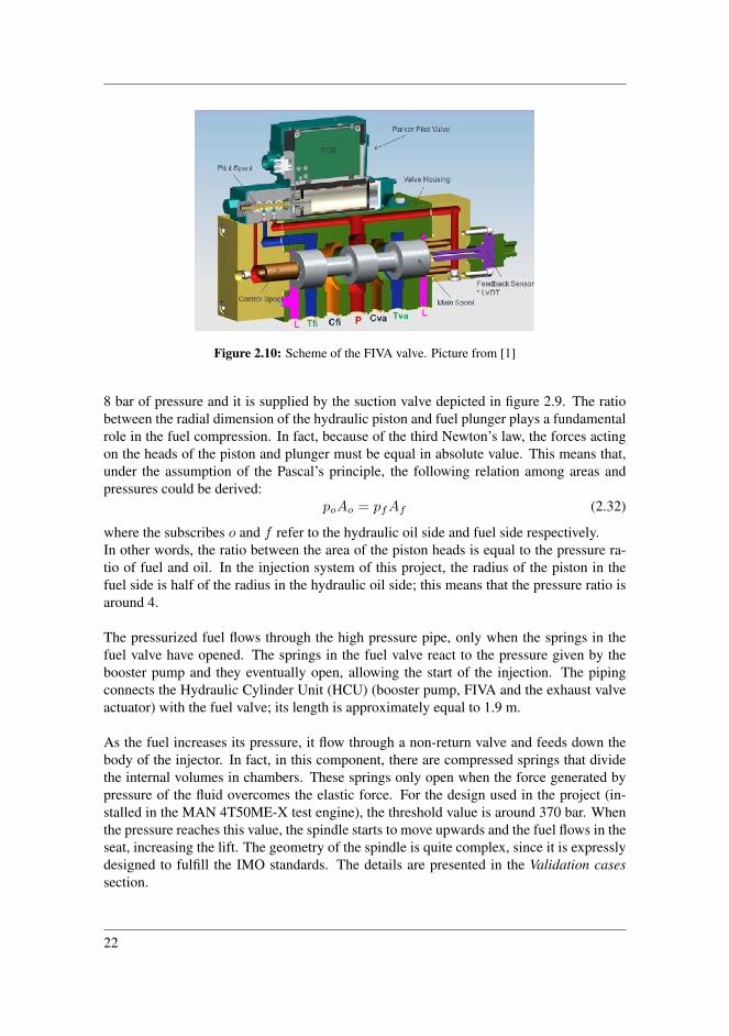
Figure 2.10: Scheme of the FIVA valve. Picture from [1]

8 bar of pressure and it is supplied by the suction valve depicted in figure 2.9. The ratiobetween the radial dimension of the hydraulic piston and fuel plunger plays a fundamentalrole in the fuel compression. In fact, because of the third Newton’s law, the forces actingon the heads of the piston and plunger must be equal in absolute value. This means that,under the assumption of the Pascal’s principle, the following relation among areas andpressures could be derived:

poAo = pfAf (2.32)

where the subscribes o and f refer to the hydraulic oil side and fuel side respectively.In other words, the ratio between the area of the piston heads is equal to the pressure ra-tio of fuel and oil. In the injection system of this project, the radius of the piston in thefuel side is half of the radius in the hydraulic oil side; this means that the pressure ratio isaround 4.

The pressurized fuel flows through the high pressure pipe, only when the springs in thefuel valve have opened. The springs in the fuel valve react to the pressure given by thebooster pump and they eventually open, allowing the start of the injection. The pipingconnects the Hydraulic Cylinder Unit (HCU) (booster pump, FIVA and the exhaust valveactuator) with the fuel valve; its length is approximately equal to 1.9 m.

As the fuel increases its pressure, it flow through a non-return valve and feeds down thebody of the injector. In fact, in this component, there are compressed springs that dividethe internal volumes in chambers. These springs only open when the force generated bypressure of the fluid overcomes the elastic force. For the design used in the project (in-stalled in the MAN 4T50ME-X test engine), the threshold value is around 370 bar. Whenthe pressure reaches this value, the spindle starts to move upwards and the fuel flows in theseat, increasing the lift. The geometry of the spindle is quite complex, since it is expresslydesigned to fulfill the IMO standards. The details are presented in the Validation casessection.

22

Chapter 3Model and implementation

The aim of this chapter is to present and comment the main models and solvers of thisMaster thesis. The simulations are run in STAR CCM+, which is one of the most popularsofware for CFD; it was developed by CD-Adepco and, nowadays, it is owned by Siemens.STAR CCM+, which stands for Simulation of Turbulent flow in Arbitrary Region - Com-putational Continuum Mechanics, uses the finite volume method to solve the conservationequations in unstructured meshes. This presentation, after a brief discussion of the gov-erning equations, follows the workflow presented in the software when a new simulationis launched.

3.1 The governing equationsIn fluid mechanics, the governing equations are based on the mass and momentum conser-vation. The derivation of the governing equations is here omitted but the reader could referto any books about fundamentals of fluid mechanics; good references are Kundu et al. [31]and Peric et al. [20]. The derivation is based on Reynolds’ transport theorem, which es-tablishes the link between a the control mass system (CM) and the control volume system(CV). Let us be φ any intensive propriety:

ddt

∫ΩCM

ρφ dΩ =ddt

∫ΩCV

ρφ dΩ +

∫SCV

ρφ(u− ub) · n dS (3.1)

where ΩCM is the volume occupied by the control mass system, ΩCV and SCV are thevolume of the control volume system and its surface, n is the outpointing normal vector,u is the velocity of the fluid and ub is the velocity of the control volume.

The popular integral form of the mass conservation could be calculated for φ = 1, whenub = 0:

∂

∂t

∫Ω

ρ dΩ +

∫S

ρu · n dS = 0 (3.2)

23

Through the use of the Gauss’ theorem and with the assumption that the control volume isinfinitely small, the differential form of the continuity equation might be derived:

∂ρ

∂t+∇ · (ρu) = 0 (3.3)

The momentum conservation is derived from the Newton’s second law and using theReynolds’ transport theorem. In general, with the aim of counting the surface stresses onthe control volume, the assumption of Newtonian fluid is made and the following integralexpression is obtained:

∂

∂t

∫Ω

ρu dΩ +

∫S

ρuu · n dS =

∫S

T · ndS +

∫Ω

ρbdΩ (3.4)

where b is the vector of the body forces and T is the stress tensor. In case of Newtonianfluid, it is defined:

T = −(p+

2

3µ∇ · u

)I + 2µ

(1

2

[∇u + (∇u)T

])(3.5)

and I is the identity tensor.The differential form of the momentum conservation could be obtained applying the Gauss’theorem to the convective and diffusive terms of eq. (3.4):

∂(ρu)

∂t+∇ · (ρuu) = ∇ · T + ρb (3.6)

Using the Cartesian coordinates and with the assumption that the gravity is the only bodyforce, eq. (3.6) could be written in index (Einstain) notation, as follows:

∂(ρui)

∂t+∂(ρuiuj)

∂xj=∂τij∂xj− ∂p

∂xj+ ρgi (3.7)

The eqs. (3.3) and (3.4) are discretized using the Finite Volume Method. This methodconsists in dividing the entire domain in smaller control volumes through a suitable grid(or mesh); the computational node is usually located in the centroid of the cell. A genericconservation equation must be valid not only for the entire volume but also for the smallcontrol volumes. Let us consider a generic control volume in three dimensions. The netflux through the surface of the cell is equal to the sum of the fluxes through each of itsface: ∫

S

f dS =∑S

∫Sk

f dS (3.8)

where f might be the component of the convective of diffusive flux normal to the referenceface. Unfortunatley, the value of f on the surface Sk is unknown being the informationavailable only in the centroid of the control volume. For this reason, the approximationof f in the face is necessary and several methods are studied in literature. In this project,both the convective and diffusive component of the flux vector in the normal direction isapproximated using a second-order scheme.

24

As regards the integration of the terms over a volume, the simplest second-order accurateapproximation consists in multiplying the mean value of the function by the volume of thecells; in symbols: ∫

Ω

q dΩ = q∆Ω ≈ qP∆Ω (3.9)

where q is a generic function and qP is the value of the function at the center of the cell.Here, the information is available and no interpolation is needed. Again, being out of thescope of this project to present in detail the Finite Volume Method and the implementationof the equation in a CFD code, this authors suggests to refer to Peric et al. [20] or thelecture notes by Bingham et al. [11].

3.2 The Segregated Flow SolverThe software STAR CCM+ offers two possibilities to solve the conservation equations pre-sented in the previous section. They are named Segregated flow solver and Coupled flowsolver. As their names suggest, they approach the problem in different manners. The Seg-regated flow solver solves for the velocity components (u, v, w) and the pressure (p) ina sequential manner; on the contrary, in the Coupled flow solver, the continuity and mo-mentum equations are solved simultaneously. Since the software only permits to use theVolume of Fraction (VOF) method with the Segregated flow solver, in this paragraph theemphasis is focused on this method. In case of interests, the author suggests to refer to theUser Guide of STAR CCM+ [45].

The Segregated flow solver uses a predictor-corrector approach to couple the pressure andvelocity to fulfill the continuity and momentum equations. The user of STAR CCM+can choose among two algorithms: SIMPLE (Semi-Implicit Method for Pressure LinkedEquations) and PISO (Pressure-Implicit with Splitting of Operators). The SIMPLE algo-rithm is the one used in the simulations since it is the only one compatible with the VOFapproach.

A brief presentation of the SIMPLE algorithm is here introduced. Solving the discretizedcontinuity and Navier-Stokes equations for the three components of velocity and pressureis complex. The main reason is the lack of an independent equation for the pressure; infact, only the pressure gradient (and not the pressure function) appears in the momentumequations. Moreover, the continuity equation is more a kinematic restriction rather than adynamic equation. In the years, as reported by Peric [20], in order to overcome this issue,the most popular approaches consist in formulating the pressure field in order to fulfillmass conservation. Under these circumstances, the SIMPLE algorithm was formulatedin early 1970s by Spalding and Patankar [40]. The discussion presented is inspired fromthe OpenFOAM blog [4]. Let us assume a steady, incompressible and laminar flow. Theconservation equations in vector form are:

∇ · u = 0 (3.10)

u · ∇u−∇ · ν∇u = −∇p (3.11)

25

where, in this context, p is the kinematic pressure (p/ρ).

The discretized momentum equation (using, for instance, the Finite Volume Method) couldbe expressed as follows:

Mu = −∇p (3.12)

whereM is a matrix having constant entries whose values only depend on the decompos-ing method. It is clear thatM has a dimension equal to the number of cells in the mesh.To recap, only the coefficients Mij are known in equation (3.12).The matrix M could now be decomposed in a diagonal matrix, A and in a off-diagonalmatrix,H, so that:

Au−H = −∇p (3.13)

This operation is aimed at obtaining a matrix which is easy to invert, A.H could be easily calculated as:

H =Mu−Au (3.14)

Rearranging equation (3.13), the velocity is now:

u = A−1H−A−1∇p (3.15)

Substituting the equation (3.15) in the continuity equation:

∇ · (A−1H−A−1∇p) = 0 (3.16)

and, finally, the Poisson equation for pressure is obtained:

∇ · (A−1∇p) = ∇ · (A−1H) (3.17)

Now that the equations (3.12) and (3.17) are obtained, the SIMPLE algorithm follows theprocedure here described:

1. The value for the pressure gradient is initialised.

2. The momentum equation (3.12) is solved for the velocity field. In general, the ve-locity field will not fulfill the mass conservation.

3. The Poisson equation (3.17) is solved for the pressure field.

4. The velocity field is corrected through equation (3.15).

5. Now the continuity equation is satisfied but the momentum equation is not fulfilledanymore. The new loop starts for point 2 until a threshold value for the error in theconservation equations is reached.

In case of turbulent flow, additional equations must be fulfilled in the loop. For instance,using URANS and k − ω turbulent model, the equation for the turbulent kinetic energyand the specific rate of dissipation are:

Mkk = Sk and Mωω = Sω (3.18)

This is a brief simplified description since it neglects for instance the under-relaxationfactors. It is out of the scope of this work to describe in depth the algorithm; again refer toPeric [20] to a more exhaustive discussion.

26

3.3 The Volume of Fluid (VOF) MethodThe Volume of Fluid (VOF) is a popular numerical method used to simulate immiscibleflow. It is a multiphase model and it requires an Eulerian framework. Its main assumptionis that the interface proprieties could be derived as function of the volume fraction of thephases in the domain. Referring to a control volume, the volume fraction of the phase i isdefined as:

αi =ViV

(3.19)

where Vi is the volume occupied by the phase i in the cell and V is the total volume of thecell.It is clear that the sum of all the phases in the same cell must be equal to 1; in symbols:

N∑i

αi = 1 (3.20)

where, in this context, N is total number of phases.

Once that the volume fraction of the different phases are known in the same cell, thephysical propriety of the mixture could be calculated. The method is reported for thedensity:

ρ =∑i

αiρi (3.21)

and dynamic viscosity:µ =

∑i

αiµi (3.22)

The introduction of the volume fraction requires an additional equation in order to obtaina close problem. At this point, neglecting the Reynolds stresses that will be treated in theTurbulent Model paragraph and considering two phases (liquid and vapour for instance),the number of unknown is 5 (three components of the velocity vector, the pressure andthe volume fraction), while the number of equation is 4 (continuity equation and the threemomentum equations). The additional equation, the phase mass conservation, is herereported:

∂

∂t

∫Ω

αi dΩ +

∮Si

αiu · n dS =

∫Ω

(Sαi− αiρi

DρiDt

)dΩ−

∫Ω

1

ρi∇ · (αiρiud,i) dΩ

(3.23)where u is the mixture (mass-averaged) velocity, ud,i is the diffusion velocity of the ith

phase; Sαiis the source term; D

Dt is the Lagrangian derivative.

In the simulation, the diffusion velocity is neglected, and so it is the last integral too.Moreover, when the fluids are incompressible, the time derivative of the density is null.

The total mass conservation could be expressed as follows:

∂

∂t

(∫Ω

ρ dΩ

)+

∮S

ρu · n dS =

∫Ω

S dΩ (3.24)

27

where the source term S is equal to the sum of the source terms of all the phases:

S =∑i

Sαiρi (3.25)

The vectorial momentum equation is

∂

∂t

(∫Ω

ρu dV)

+

∮S

ρu× u · ndS =

∮S

pI · n dS +

∮A

T · n dS +

∫Ω

ρg dΩ+

+

∫Ω

bdΩ−∑i

∫S

αiρiud,i × ud,i · n dS

(3.26)

where I is the unit tensor, T is the stress tensor and b is the vector of body forces.

3.4 The Cavitation ModelThe phase and mass conservation from the eqs. (3.24) and (3.26) of the previous sectionrequire the knowledge of a source term. In this project, this source is responsible to thephase change due to cavitation. In STAR CCM+, there are three cavitation models: FullRayleigh-Plesset model, Schnner-Sauer model and Homogeneous Relaxation model. Eachof them has some peculiarities and it models the bubbles growth rate in different manners.

The Full Rayleigh-Plesset model implements the Rayleigh-Plesset equation presented inthe Theory section in eq. (2.31). The Schnner-Sauer model is a simplification of the pre-vious model, where the bubble growth acceleration and the viscous and tension effects areneglected. Lastly, the Homogeneous Relaxation model is based on a finite rate equationwith an empirical time scale formulation [45]. In this work, only the first two cavitationmodels are applied. In fact, the Homogeneous Relaxation model is not recommended forthe project (the Userguide [45] reports that it is suitable for modeling phenomenon whichoccur in thermal non-equilibrium). Moreover, Brenner [14] reports that, in engineeringapplication, the results from the Schnerr-Sauer model are comparable with those obtainedapplying the Rayleight-Plesset model. This statement will be test further in the projectwhen both of the models will be implemented.

All the cavitation models in STAR CCM+ are based on homogeneous distribution of thenucleation sites; they are also called seeds in the software. One of the parameters that theuser needs to set is the density of seeds per unit of volume, n0 (Seed density). The modelassumes that these seeds are spherical and uniformly distributed in the volume, moreover,all seeds have initially the same radius, R0. This is the the second parameter that must beset by the user, in the software it is named Seed diameter, D0 = 2R0. The initial radiuscorresponds also to the smallest value of the radius that the bubble could assume in thedomain during the simulation. Another important assumption is that the number of seedsin a control volume is proportional to the volume of liquid. The amount of seeds in thiscontrol volume is thus:

N = n0αLV (3.27)

28

where αL is the the volume fraction of liquid.

The total amount of vapour, under the assumption of spherical bubbles, is:

VV = N

(4

3R3π

)(3.28)

and the phase fraction of vapour:

αV =VVV

= n0αL

(4

3R3π

)(3.29)

Therefore, once that the volume fraction of liquid and vapour are known, the local radiuscould be calculated, inverting equation (3.29):

R =

(3αV

4n0αLπ

) 13

(3.30)

At these point, the user should be aware that the density of seeds and the seed diameterhave not a physical meaning. They are simply used to tune-up the physical model andestablish a satisfying agreement with the eventual experimental values. In his Masterthesis, Andersen [5] reported the following tables of recommended values in case of mainphase is diesel fuel; it was taken from the PhD thesis by Giannadakis [23].

n0 [1/m3] R0 [m] α0

Range of recommended values 1012, 1014 0.3 10−6, 2 10−6 5 10−6, 5 10−5

Table 3.1: Recommended values for the initial parameter of the cavitation model suggested byGiannadakis [23]

Lastly, the mass transfer per unit of volume is:

m = ρVdVVdt

1

V= ρV

ddt

(N

4

3πR3

)1

V= 4ρV n0αLπR

2 dRdt

(3.31)

Now, the above-mentioned models differ by the method used to calculate the radial bubblegrowth, dR/dt, in eq. (3.31). The Schnner-Sauer model estimates this quantity from theRayleigh-Plesset equation, neglecting the bubble growth acceleration, the viscous termand the surface tension: (

dRdt

)2

=2

3

(psat − p∞

ρL

)(3.32)

where p∞ is the surrounding pressure. When the saturation pressure is larger than thesurrounding pressure, the radial bubbles’ growth is positive:

dRdt

=

√2

3

(psat − p∞

ρL

)(3.33)

29

On the contrary, when the surrounding pressure is larger than the saturation pressure:

dRdt

= −

√2

3

(p∞ − psat

ρL

)(3.34)

In general:

dRdt

= sign(psat − p)

√2

3

(|p∞ − psat|

ρL

)(3.35)

Substituting eq. (3.35) in eq. (3.31), the mass transfer per unit of volume is:

m = 4ρvn0αlπR2sign(psat − p)

√2

3

(|p− psat|

ρL

)(3.36)

Lastly, the source term in eq. 3.24 is:

SV = 4n0αlπR2sign(psat − p)

√2

3

(|p− psat|

ρL

)(3.37)

3.5 The Temporal DiscretizationThe problem of this project is transient, this means that the additional variable time must betaken into account. In order to approximate the time derivative of any physical quantity,several methods could be used. In engineering application, the most popular is ImplicitEuler; it is implemented in STAR CCM+ and it is applied in the all the simulations of thisproject.

Depending on the stencil, the user of the software might choose among the first and secondorder accuracy schemes. The first order time discretization uses the solution of the current(tm+1) and previous (tm) timestep; in other words, the stencil contains two points. Thetime derivative of the generic function φ(t) evaluated at time step tm+1 is:

dφ(t)

dt=φ(tm+1)− φ(tm)

∆t(3.38)

In the second order accuracy scheme, the stencil counts three points; in addition of thesolution at level tm+1 and tm, the value of the function at time tm−1 is needed too:

dφ(t)

dt=

32φ(tm+1)− 2φ(tm) + 1

2φ(tm−1)

∆t(3.39)

The choice of the time-step ∆t is based on the Courant-Friedrichs-Lewy (often abbre-viated as CFL) condition, which establishes the condition for convergence when partialdifferential equations are solved. In CFD, the time step is calculated from the definition ofthe Courant number:

C =u∆t

∆x(3.40)

This non dimensional number must be smaller than 1 to ensure that the information is notpropagating through more than cell in the given time-step. Values higher than 1 might leadto instabilities and the solution might not be reliable.

30

3.6 The Turbulence ModelIn all the simulations, the Reynolds number is expected to be higher than the critical value.In fact, the laminar limit for a flow in pipe, which could be considered a simplified modelof a nozzle hole, is around 2,000 while the expected Reynolds number has an order ofmagnitude at least equal to 106. Therefore, the flow is turbulent and the Reynolds stressesmust be taken into account. It is not the purpose of this work to discuss in detail the turbu-lence modelling; please refer to Wilcox [49] for a very detailed analysis with the focus onthe implementation in CFD codes.

The signal of every fluid-dynamic quantity in a turbulent flow could be decomposed inmean value and fluctuating component. With this in mind, consider the horizontal compo-nent of the velocity vector, u:

u = u+ u′ (3.41)

where u refers to the mean value and u′ to the fluctuating component. Note that, bydefinition, u′ = 0. The procedure of decomposing the signal in mean value and fluctuatingcomponent is called Reynolds decomposition. When the three components of the velocityvector and the pressure are decomposed as above, and they are inserted in the Navier-Stokes equations, eq. (3.7), one could get the following expression (known as UnsteadyReynolds Average Navier-Stokes equation, or more simply, URANS):

ρ

(∂ui∂t

+ uj∂ui∂xj

)= ρgi +

∂

∂xj

(τij − ρu′iu′j

)(3.42)

The main difference from eq. (3.7) is the presence of the terms −ρu′iu′j in the right handside brackets. They come from the convective term of the Navier-Stokes equation:

∂

∂xj(ρuiuj) = ρuj

∂ui∂xj

+∂

∂xj

(ρu′iu

′j

)(3.43)

The terms −ρu′iu′j are the components of a symmetric second order tensor (9 entries butonly 6 independent) and they might be interpreted as additional stresses due to turbulence.This is the reason why they are called Reynolds stresses and they are merged with theviscous stresses in eq. (3.42), even though they originate from the convective term, in theleft hand side of the Navier-Stokes equation.

At this point, there are four equations (continuity and three Reynolds Averaged NavierStokes equations) but ten unknowns (pressure, three components of velocity and the sixReynolds stresses); it means that the problem is not closed. Consequently, methods tocompute the terms u′iu

′j have been developed. In literature, the turbulence models could

be classified in three families: algebraic models, turbulence-energy equations model andsimulation models, which includes Large Eddies Simulation (LES) and Detached EddiesSimulation (DES). In this project, only the turbulence-energy models are used becausethey offer the best compromise between computational time and precision. Indeed, theLES and DES require that the number of grid point to resolve the smallest length-scale ofturbulence (Kolmogoroff’s length scale) is proportional to Re3 [36]. For high Reynolds

31

number (≈ 106), the domain require a tremendously large number of cells. This is thereason why these turbulence models are only used for simple geometry and small scales.

The most common turbulence-energy models are based on two additional equations. Be-cause of that, they are named k− ε model and k−ω model, where k refers to the turbulentkinetic energy, ε is the rate of dissipation of turbulent energy and ω is the specific dissipa-tion rate. STAR CCM+ provides the possibilities to use both of these models. In particular,the k−ω model is implemented using Menter’s modification (k−ω SST), which is aimedto have higher sensibility in case of adverse pressure gradient. The software allows toscale the turbulent viscosity too, which is the analogous term of the dynamic viscosity inthe Reynolds stresses.

3.7 The Overset MeshThe overset mesh (also known as chimera) is a technique used to simulate the motion ofoverlapping meshes. The method requires one fixed mesh (commonly known as back-ground), and one (or more) moving mesh, the overset. The theoretical approach was de-veloped in 1983 by Atta and Vadyak [6] and their work represents a milestone in this field.It is not the aim of this thesis to discuss in depth the technique and the algorithm (theUser Guide [45] provides a lot of information in this sense) but the main ideas are herepresented.

The overlapping of the meshes poses a central topological problem: how is the flow fieldinformation transmitted from one mesh to another? This question is solved by the algo-rithm implemented in STAR CCM+ sorting the cells in the domain in four families: activecells, passive cells, donor cells and acceptor cells. In the active cells, as the name suggests,the discretized governing equations are solved. This does not happen in the passive cells;they are the cells in the background that are blanked out due to the motion of the oversetregion. Of course, during the simulation, depending on the position of the overset mesh,an active cell could become passive, and viceversa. The donator cells are the cells usedto provide information between the meshes; this is possible through the acceptor cells thatare located in the boundary between background and overset. They receive the interpo-lating information from the donor cells. A simple representation of how the informationare exchanged from cell to cell is depicted in figure 3.1. The background mesh is coloredin blue, while the overset is in red. From the mathematical point of view, the informationin the external cells (coloured in blue and orange and belonging respectively to the back-ground and overset) is calculated through the use of the acceptor cells. In the picture, twoacceptor cells (one in the background and the other in the overset mesh) are depicted withdashed lines. The information in the centroid of the acceptor cell is calculated from thecells in the background. In case of a 2 dimensional analysis, three background cells areused for this purpose. In three dimension, they are four. These cells are selected in a waythat the centroid of the acceptor cell is located in the triangular (in 2D) or in tetragonal (in3D) shape formed connecting the centorids of the background cells, as depicted in green inthe figure. In this way, through interpolation (STAR CCM+ provides four different meth-ods of interpolation) the information is calculated in the centroid of the acceptor cell, and

32

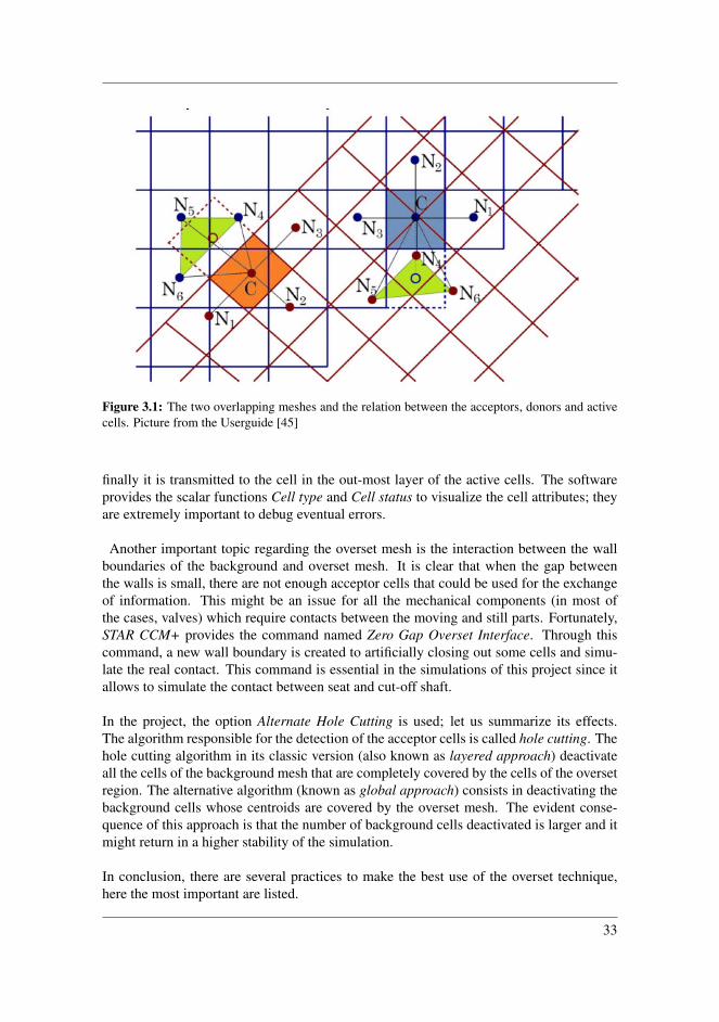
Figure 3.1: The two overlapping meshes and the relation between the acceptors, donors and activecells. Picture from the Userguide [45]

finally it is transmitted to the cell in the out-most layer of the active cells. The softwareprovides the scalar functions Cell type and Cell status to visualize the cell attributes; theyare extremely important to debug eventual errors.

Another important topic regarding the overset mesh is the interaction between the wallboundaries of the background and overset mesh. It is clear that when the gap betweenthe walls is small, there are not enough acceptor cells that could be used for the exchangeof information. This might be an issue for all the mechanical components (in most ofthe cases, valves) which require contacts between the moving and still parts. Fortunately,STAR CCM+ provides the command named Zero Gap Overset Interface. Through thiscommand, a new wall boundary is created to artificially closing out some cells and simu-late the real contact. This command is essential in the simulations of this project since itallows to simulate the contact between seat and cut-off shaft.

In the project, the option Alternate Hole Cutting is used; let us summarize its effects.The algorithm responsible for the detection of the acceptor cells is called hole cutting. Thehole cutting algorithm in its classic version (also known as layered approach) deactivateall the cells of the background mesh that are completely covered by the cells of the oversetregion. The alternative algorithm (known as global approach) consists in deactivating thebackground cells whose centroids are covered by the overset mesh. The evident conse-quence of this approach is that the number of background cells deactivated is larger and itmight return in a higher stability of the simulation.

In conclusion, there are several practices to make the best use of the overset technique,here the most important are listed.

33

Topological rule: mesh size should match as much as possible around the overset bound-ary [45]. The main reason is that it assures the most correct interpolation possible. Most ofthe issues due to the robustness and conservation could be solved in this way. In general,the user should prefer a tight fit mesh for the overset region. This shape allows to havesmaller cell counts and it permits the motion of the overset in small gaps.

Temporal discretization rule: when the time integration is set to the 1st (or 2nd) orderimplicit Euler scheme, the maximum displacement of the overset must be equal to thesmallest (or to half the smallest) cell size in the overlapping region. The difference in thescheme order is due to the time discretization; in fact, as shown in the section The Tempo-ral Discretization, the first order Euler requires the values of the previous time step, whilethe second order Euler requires the values from the previous two time steps (see eqs. (3.38)and (3.39)).

34

Chapter 4Validation cases

As reported in the previous sections, there are not experimental data of the motion of thecut-off shaft in the real injector system. Consequently, there are not information aboutthe cavitation intensity: where and how the vapor bubbles form remains an open questionthat still needs an answer. Recall that it is very difficult to reproduce experimentally theoperating condition of the injector due to the high pressure involved in the process and thevelocity of the flow inside the nozzle holes. Moreover, the small dimension of the nozzleand the need of using optical method to detect the vapour bubbles make the investigationextremely complex. This is the reason why computational fluid dynamics is an essentialtool to predict the behaviour of the fluid and, eventually, optimize the design of the injector.

The lack of the experimental data at the opening and closing of the fuel valve implies theneed of taking a step back and validating the physical models using test cases. With theaim of making everything as simple as possible but not simpler1, two validation cases areconsidered. The first of the list is about the unsteady cavitation in a converging-divergingnozzle. This test allows to gain confidence with the numerical simulation of multiphaseflows when the geometry is not too complex. The second validation case is about the singlephase flow of diesel fuel in the injector when the cut-off shaft is moving. This is possi-ble through the use of the overset technique, one of the most popular method to simulatethe motion in CFD. A more detailed description of the tests is presented in the followingsections.

4.1 Unsteady cavitation in an axisymmetric Venturi noz-zle

Time-dependant cavitation is expected in the injection system at the operating condition;for this purpose, a validation of the multiphase flow with respect to time is required. The

1The sentence in italics is attributed to Einstain (The Herbert Spencer Lecture, delivered at Oxford in June1933) and it is known as Einstain’s razor, in analogy of Occam’s razor.

35

unsteadiness of the vapor bubbles is mainly due to the displacements of the cut-off shaftand the time-dependant inlet and outlet pressures at the boundaries.

In literature, there are several experiments regarding the periodic shedding of cavitationclouds around different geometries. For instance, extensive researches have been con-ducted for cavitating hydrofoils, in the hope of studying erosion, vibration and noise pro-duced by the collapse of the vapor bubbles [35, 30]. Being an external flow, this experi-ment is not really suitable for the investigation of this Master project, where the attentionis addressed to internal flows. Internal flow means that the fluid must be bounded by asurface where the boundary layer develops. With this in mind, the simulation of the un-steady cavitating flow in a converging-diverging nozzle is performed, replicating in STARCCM+ the laboratory conditions reported in the article Dynamics of partial cavitation inan axisymmetric converging-diverging nozzle by Jahangir, Hogendoorn and Poelma [28].The numerical results will be then compared with the authors’ data.

It is relevant to mention that, even for simple geometries, the cavitation mechanisms arenot fully understood, especially as regards the onset of cavitation. The unsteadiness, theturbulence and the interaction between vapor cavities contribute to making cavitation dif-ficult to comprehend. This is the reason why experiments performed with more and morecomplex techniques are needed even in these days. It is clear that it affects the reliabilityof numerical models and, in general, it is hard to obtain results with a sufficient accu-racy. In literature, there are several articles aimed at reproducing the unsteady cavitationin two dimensional Venturi nozzle or in axisymmetric geometries. For instance, Yuanget al. [51] worked with the Volume of fluid technique and the Schnerr-Sauer cavitationmodel to model the two phase flow in an axisymmetric 2D nozzle. The authors used theURANS equation with the standard k-ε model and they reported slightly oscillation in thelocation of the cavity wake. As it will be discussed in the further sections, the turbulencemodel plays an important role in the modelling of this problem. Reboud et al. [43] andCoutier-Delgosha et al. [17] studied the influence of several turbulence model in a twodimensional Venturi-type section. In particular, noting an underestimation of the turbulentviscosity near the vapor cavity, Reboud proposed the use of a scaling factor. The only arti-cle I was able to find about the axisymmetric Venturi is by Gorkh et al. [24]. The authorsused the same geometry presented in the following section (but in 3-D) and they were ableto simulate the re-entrant mechanism for high cavitation number, σ. Unfortunately, in thepaper, many information are missing; the turbulence model is not mentioned as well as thecavitation model.

This section is organized as follows: in the first subsection, the experiment by Jahana-gir et al. [28] is presented and particular attention is addressed to the causes of the cav-itating flow. The mechanisms of the multiphase flow are described and the non dimen-sional numbers are presented. The other subsections follow the work-flow of the softwareSTAR CCM+: in the order, geometry, physics, boundary conditions, mesh and solvers.The results are described by means of pictures and plots. Lastly, in the discussion, theagreement between the numerical and experimental results is discussed.

36

Figure 4.1: Streamlines (above) and the pressure distribution (below) along the length of a onedimensional converging-diverging nozzle. The dotted line shows the onset of the multiphase flow.In case of cavitation, it is not possible to describe the pressure distribution far from the throat. Thepicture is from Hogendoorn’s Master thesis [26].

4.1.1 The Overview of the ExperimentThe experiments by Jahangir et al. [28] are aimed at detecting the periodic shedding ofcavitation clouds in a three dimensional axisymmetric converging-diverging nozzle. Thenucleation and growth of the vapor bubbles could be explained as a consequence of thevelocity increase in the throat section. This is very similar of what happens in dieselinjectors; in this regard, refer to Nurick’s one dimensional model [39] presented in theTheory chapter. Here, the physical reasons are reported again to give the picture of thephenomenon in a Venturi nozzle.

With the assumption of steady, incompressible, single phase flow, and neglecting the grav-ity, Bernoulli’s equation might be applied along a streamline:

1

2ρu2 + p |along a streamline = const. (4.1)

Since the velocity reaches its maximum in the throat, here, the pressure might drop underthe saturation limit at operating temperature. Therefore, the throat is the critical sectionwhere the onset of cavitation might occur.A nice representation of the streamlines and pressure distribution in a one dimensionalmodel is depicted in figure 4.1. Here, three pressure functions are depicted with the aim ofvisualizing as many different conditions. If the pressure along the symmetry axis is alwaysabove the saturation condition, cavitation will not occur. The onset of cavitation beginswhen, at least in one point, the pressure reaches the critical value: p(x) = psat. As it wasstated before, the coordinate x corresponds to the neck of the Venturi nozzle. Lastly, whena multiphase flow is expected, it is impossible to predict the trend of the pressure function

37

with respect of the x-coordinate.

In order to study different cavitation regimes, Jahanguir et al. [28] performed several ex-periments varying the outlet pressure. To explain their procedure, it is useful to recall oneof the definitions of the cavitation number introduced in the Theory chapter:

σ =p− psat

12ρu

20

(4.2)

In a converging-diverging nozzle, p refers to the outlet static pressure (in other context, itmight be the inlet static pressure) and u0 is the flow velocity at the throat. Hogendoorn [26]pointed out that the outlet static pressure is the driving force of the cavitation in a Venturi.Let us consider a situation where the inlet pressure is fixed. A large outlet pressure (but, ofcourse, lower then the inlet pressure) implies a low ∆p between inlet and outlet and lowvelocity at the throat because of eq. (4.1). In these circumstances, cavitation is not likely tooccur and the cavitation number σ is large. On the contrary, low outlet pressure implies anhigh driving force, high flow velocity through the neck section and a tumultuous cavitationregime. This situation is described by a low cavitation number, σ.

In literature, depending on the cavitation number, three cavitation mechanisms are de-scribed in a Venturi nozzle. They are the re-entrant jet mechanism, side entrant jet mecha-nism and bubble shock mechanisms. In this validation case, the re-entrant jet mechanismis considered. It is the first (discovered in 1955 by Knapp [29]) and most studied mecha-nism. Moreover, it is relevant to this project since it was observed at the inlet of nozzlesholes in diesel injectors too. In this regard, Sato and Saito [44] observed periodic cavitiesof vapor in a circular cylindrical nozzles. The authors noted that the bubbles grew untilthey reached a characteristic length, Lcav , after that, a portion of the bubble was set apartand it was advected by the surrounding flow. More recently, the same phenomenon wasobserved in the experiments by Stanley et al. [47].

A brief presentation of the re-entrant jet mechanism is here discussed. The cycle couldbe described in four time-steps:

- A cavity forms at the end of the breaking cycle in the throat of the Venturi nozzle.The bubble clouds (which is set apart from the previous cycle) is advected throughthe diverging section of the nozzle.

- When the cavity reaches its maximal length (Lcav), a re-entrant jet begins to form.As reported in several papers ([30], [15]), the re-entrant jet is due to the impingementof the fluid surrounding the vapor cavity on the wall.

- The re-entrant stream reaches the throat of the Venturi nozzle and a part of the cavityis set apart. A bubble cloud now is formed.

- The bubble cloud is advected while a new cavitation sheet begins to form again.

In figure 4.2, the four steps of the break-off cycle are depicted in a converging-divergingnozzle.

38

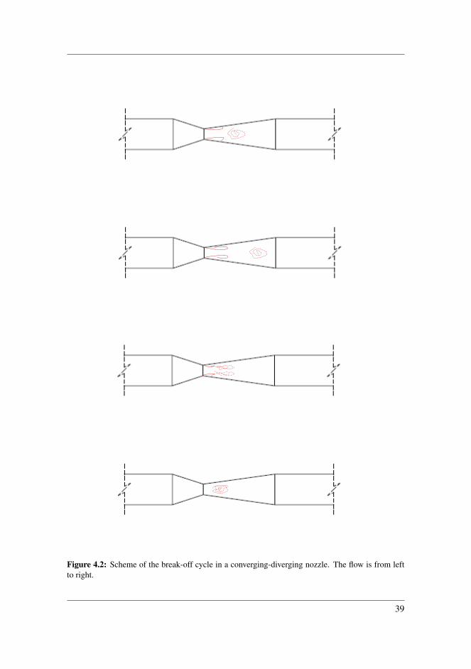
Figure 4.2: Scheme of the break-off cycle in a converging-diverging nozzle. The flow is from leftto right.

39

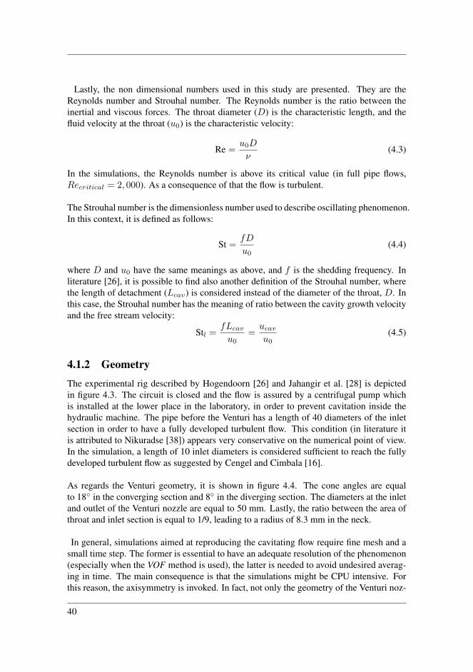
Lastly, the non dimensional numbers used in this study are presented. They are theReynolds number and Strouhal number. The Reynolds number is the ratio between theinertial and viscous forces. The throat diameter (D) is the characteristic length, and thefluid velocity at the throat (u0) is the characteristic velocity:

Re =u0D

ν(4.3)

In the simulations, the Reynolds number is above its critical value (in full pipe flows,Recritical = 2, 000). As a consequence of that the flow is turbulent.

The Strouhal number is the dimensionless number used to describe oscillating phenomenon.In this context, it is defined as follows:

St =fD

u0(4.4)

where D and u0 have the same meanings as above, and f is the shedding frequency. Inliterature [26], it is possible to find also another definition of the Strouhal number, wherethe length of detachment (Lcav) is considered instead of the diameter of the throat, D. Inthis case, the Strouhal number has the meaning of ratio between the cavity growth velocityand the free stream velocity:

Stl =fLcavu0

=ucavu0

(4.5)

4.1.2 GeometryThe experimental rig described by Hogendoorn [26] and Jahangir et al. [28] is depictedin figure 4.3. The circuit is closed and the flow is assured by a centrifugal pump whichis installed at the lower place in the laboratory, in order to prevent cavitation inside thehydraulic machine. The pipe before the Venturi has a length of 40 diameters of the inletsection in order to have a fully developed turbulent flow. This condition (in literature itis attributed to Nikuradse [38]) appears very conservative on the numerical point of view.In the simulation, a length of 10 inlet diameters is considered sufficient to reach the fullydeveloped turbulent flow as suggested by Cengel and Cimbala [16].

As regards the Venturi geometry, it is shown in figure 4.4. The cone angles are equalto 18 in the converging section and 8 in the diverging section. The diameters at the inletand outlet of the Venturi nozzle are equal to 50 mm. Lastly, the ratio between the area ofthroat and inlet section is equal to 1/9, leading to a radius of 8.3 mm in the neck.

In general, simulations aimed at reproducing the cavitating flow require fine mesh and asmall time step. The former is essential to have an adequate resolution of the phenomenon(especially when the VOF method is used), the latter is needed to avoid undesired averag-ing in time. The main consequence is that the simulations might be CPU intensive. Forthis reason, the axisymmetry is invoked. In fact, not only the geometry of the Venturi noz-

40

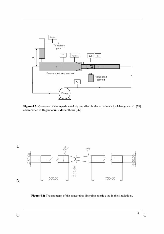
Figure 4.3: Overview of the experimental rig described in the experiment by Jahanguir et al. [28]and reported in Hogendoorn’s Master thesis [26].

50,0

0

50,0

0

18° 8°

16,66

500,00 730,00

A A

B B

C C

D

E

4 3 2 1

DRAWN

CHK'D

APPV'D

MFG

Q.A

UNLESS OTHERWISE SPECIFIED:DIMENSIONS ARE IN MILLIMETERSSURFACE FINISH:TOLERANCES: LINEAR: ANGULAR:

FINISH: DEBURR AND BREAK SHARP EDGES

NAME SIGNATURE DATE

MATERIAL:

DO NOT SCALE DRAWING REVISION

TITLE:

DWG NO.

SCALE:1:20 SHEET 1 OF 1

A4

WEIGHT:

Venturi

Figure 4.4: The geometry of the converging-diverging nozzle used in the simulations.

41

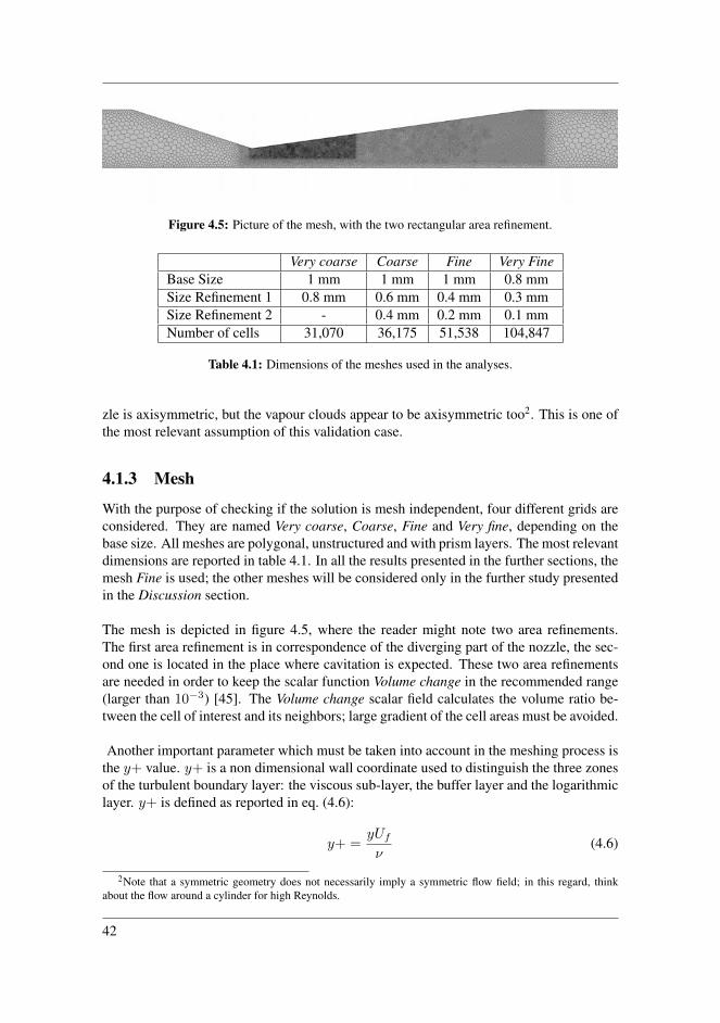
Figure 4.5: Picture of the mesh, with the two rectangular area refinement.

Very coarse Coarse Fine Very FineBase Size 1 mm 1 mm 1 mm 0.8 mmSize Refinement 1 0.8 mm 0.6 mm 0.4 mm 0.3 mmSize Refinement 2 - 0.4 mm 0.2 mm 0.1 mmNumber of cells 31,070 36,175 51,538 104,847

Table 4.1: Dimensions of the meshes used in the analyses.

zle is axisymmetric, but the vapour clouds appear to be axisymmetric too2. This is one ofthe most relevant assumption of this validation case.

4.1.3 Mesh

With the purpose of checking if the solution is mesh independent, four different grids areconsidered. They are named Very coarse, Coarse, Fine and Very fine, depending on thebase size. All meshes are polygonal, unstructured and with prism layers. The most relevantdimensions are reported in table 4.1. In all the results presented in the further sections, themesh Fine is used; the other meshes will be considered only in the further study presentedin the Discussion section.

The mesh is depicted in figure 4.5, where the reader might note two area refinements.The first area refinement is in correspondence of the diverging part of the nozzle, the sec-ond one is located in the place where cavitation is expected. These two area refinementsare needed in order to keep the scalar function Volume change in the recommended range(larger than 10−3) [45]. The Volume change scalar field calculates the volume ratio be-tween the cell of interest and its neighbors; large gradient of the cell areas must be avoided.

Another important parameter which must be taken into account in the meshing process isthe y+ value. y+ is a non dimensional wall coordinate used to distinguish the three zonesof the turbulent boundary layer: the viscous sub-layer, the buffer layer and the logarithmiclayer. y+ is defined as reported in eq. (4.6):

y+ =yUfν

(4.6)

2Note that a symmetric geometry does not necessarily imply a symmetric flow field; in this regard, thinkabout the flow around a cylinder for high Reynolds.

42

ρ [kg/m3] µ [Pa s] γ [N/m] psat [Pa]Water 998.2 0.001001 0.072 2339Vapor 0.01731 9.7272 10−6 - -

Table 4.2: Physical proprieties of water and water vapor at T = 20.

where Uf is the friction velocity. The friction velocity is defined as the square root of theratio between the wall shear stress (τ0) and the density:

Uf =√τ0/ρ. (4.7)

In order to have a full resolution of the turbulent boundary layer including the viscoussub-layer, it is required that y+ ≈ 1. This condition might be important in the reliabilityof the results since the re-entrant jet develops close to the walls.

4.1.4 PhysicsThe problem is approached using the solver Segregated Flow and the Eulerian multiphaseapproach Volume of Fluid (VOF). As suggested by the Userguide [45], the two phases aresimulated as incompressible fluids. It is worthwhile to mention that the compressibilityeffects of the liquid are negligible since the velocity is far below the speed of sound. Inparticular, it is less than 0.3 Mach, the threshold value from which the compressabilityeffects starts to be relevant. The experiments are performed at constant temperature, thus,the thermal effects are neglected. In other words, the equation of state and the energyequations are not required.

STAR CCM+ demands in input the following physical proprieties for the liquid and gasphases: density, dynamic viscosity, saturation pressure and surface tension (only whenthe full Rayleigh-Plesset cavitation model is enabled). The numerical values are retrievedusing the software EES-Engineering Equation Solver, which stores the thermodynamicproprieties of the most common fluids. In the experiments, the operating fluid is water atroom temperature. Since it is not explicitly stated in the article by Jahanguir et al. [28], thetemperature is set equal to 20C (standard conditions). The physical proprieties of waterand water vapor are summarized in the table 4.2.

As regards the cavitation modelling, both the Schnerr-Sauer and full Rayleigh-Plessetmodels are used. Regardless of which cavitation model is used, STAR CCM+ requires twoparameters in input: the seed density (n0) and the seed diameter (d). At this point, it isrelevant to mention that these parameters have not physical meanings: they are used totune-up the simulations.

Incidentally, the way in which the seed density and diameter are defined in the User-guide [45] might lead to misunderstandings. In fact, the seed density and the seed di-ameter might be evaluated experimentally in the laboratory, since impurities are need asnucleation site for the vapor cavities. In general, they are small bubbles of air or otherimmiscible gases [14]. Unfortunately, there is not correlation between the seed density

43

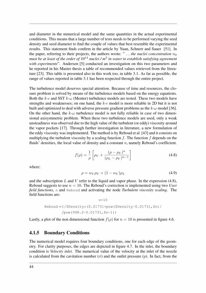
and diameter in the numerical model and the same quantities in the actual experimentalconditions. This means that a large number of tests needs to be performed varying the seeddensity and seed diameter to find the couple of values that best resemble the experimentalresults. This statement finds confirm in the article by Yuan, Schnerr and Sauer [51]. Inthe paper, referring to their projects, the authors wrote: ” . . . the nuclei concentration n0

must be at least of the order of 1014 nuclei / m3 in water to establish satisfying agreementwith experiments”. Andersen [5] conducted an investigation on this two parameters andhe reported in his Master thesis a table of recommended values retrieved from the litera-ture [23]. This table is presented also in this work too, in table 3.1. As far as possible, therange of values reported in table 3.1 has been respected through the entire project.

The turbulence model deserves special attention. Because of time and resources, the clo-sure problem is solved by means of the turbulence models based on the energy equations.Both the k-ε and SST k-ω (Menter) turbulence models are tested. These two models havestrengths and weaknesses; on one hand, the k-ε model is more reliable in 2D but it is notbuilt and optimized to deal with adverse pressure gradient problems as the k-ω model [36].On the other hand, the k-ω turbulence model is not fully reliable in case of two dimen-sional axisymmetric problem. When these two turbulence models are used, only a weakunsteadiness was observed due to the high value of the turbulent (or eddy) viscosity aroundthe vapor pockets [17]. Through further investigation in literature, a new formulation ofthe eddy viscosity was implemented. The method is by Reboud et al. [43] and it consists onmultiplying the turbulent viscosity by a scaling function f . The function f depends on thefluids’ densities, the local value of density and a constant n, namely Reboud’s coefficient.

f(ρ) =1

ρ

[ρV +

(ρ− ρV )n

(ρL − ρV )n−1

](4.8)

where:ρ = αV ρV + (1− αV )ρL (4.9)

and the subscription L and V refer to the liquid and vapor phase. In the expression (4.8),Reboud suggests to use n = 10. The Reboud’s correction is implemented using two Userfield functions, n and Reboud and activating the node Turbulent viscosity scaling. Thefield functions are:

n=10

Reboud =1/$Density*(0.01731+pow($Density-0.01731,$n)/

/pow(998.2-0.01731,$n-1))

Lastly, a plot of the non dimensional function f(ρ) for n = 10 is presented in figure 4.6.

4.1.5 Boundary Conditions

The numerical model requires four boundary conditions, one for each edge of the geom-etry. For clarity purposes, the edges are depicted in figure 4.7. In the inlet, the boundarycondition is Velocity inlet. The numerical value of the velocity at the inlet of the nozzleis calculated from the cavitation number (σ) and the outlet pressure (p). In fact, from the

44

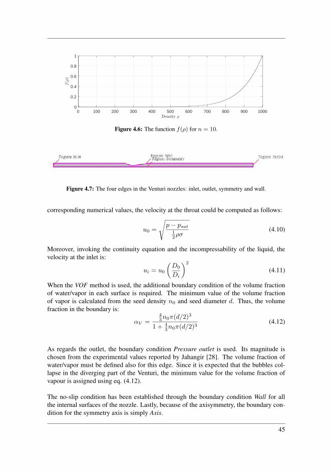
0 100 200 300 400 500 600 700 800 900 1000

0

0.2

0.4

0.6

0.8

1

Figure 4.6: The function f(ρ) for n = 10.

Figure 4.7: The four edges in the Venturi nozzles: inlet, outlet, symmetry and wall.

corresponding numerical values, the velocity at the throat could be computed as follows:

u0 =

√p− psat

12ρσ

(4.10)

Moreover, invoking the continuity equation and the incompressability of the liquid, thevelocity at the inlet is:

ui = u0

(D0

Di

)2

(4.11)

When the VOF method is used, the additional boundary condition of the volume fractionof water/vapor in each surface is required. The minimum value of the volume fractionof vapor is calculated from the seed density n0 and seed diameter d. Thus, the volumefraction in the boundary is:

αV =43n0π(d/2)3

1 + 43n0π(d/2)3

(4.12)

As regards the outlet, the boundary condition Pressure outlet is used. Its magnitude ischosen from the experimental values reported by Jahangir [28]. The volume fraction ofwater/vapor must be defined also for this edge. Since it is expected that the bubbles col-lapse in the diverging part of the Venturi, the minimum value for the volume fraction ofvapour is assigned using eq. (4.12).

The no-slip condition has been established through the boundary condition Wall for allthe internal surfaces of the nozzle. Lastly, because of the axisymmetry, the boundary con-dition for the symmetry axis is simply Axis.

45

4.1.6 SolverAs reported in the chapter Model, the only solver compatible with the VOF method isSegregated flow. The time discretization is Euler Second Order and the time step is∆t = 10−6 s. The choice of this time step is justified by the Courant-Friedrichs-Lewyconvergence condition. The time step allows to obtain the maximum Courant number be-low 1 in all the cells of the domain.

In order to avoid the risk of divergence, the flow is initialized disabling the cavitationmodel. This has been achieved through two User field functions. The former resets the va-por source term in the transport equation when the time is below an user-defined thresholdgiven by the latter function. The value used in the simulation is ∆t = 10−3 s. The sourceterm is set equal to zero through the option ScalingFac+ (which is a scaling factor forthe source term) in the Schnerr-Sauer cavitation model. The just-mentioned field functionStartCavitation and Cavitiation are defined as follows:

StartCavitation=1E-3; Cavitiation = (Time < $ StartCavitation)?0 : 1

This procedure is compatible only when the Schnerr-Sauer cavitation model is imple-mented. Otherwise, a single-phase flow is initialized and the cavitation model is enabledonly after that the continuity residual has reached a small value (10−6). The inner num-ber of iteration is set in order to have small residuals; tuning up the model, the value 15is used. Lastly, the stopping criteria is based on the expected frequency, and its value ischosen to be large enough to collect a significant number of periods. In all the simulation,the stopping criteria is set tstop = 80 ms.

4.1.7 ResultsThe test is performed with the outlet pressure equal to 90 kPa and cavitation number equalto σ = 1. From eqs. (4.10) and (4.11), the flow velocity at the throat and inlet sections isequal to 13.25 m/s and 1.46 m/s respectively. The Reynolds number is 2.2 105; the flow isturbulent.To check the correctness of the model, in a preliminary analysis, the cavitation model isdisabled and the single phase flow is analyzed, focusing on the pressure and velocity dis-tribution. The numerical value of the mass flow has been compared with the theoreticalvalue. Once that the results matched, the cavitation model is enabled. Because of the widerange of values which the free parameter (seed density and seed diameter) could assumeand the time required to run each simulation, a Guess-and-Test approach is used to have asatisfying agreement with the experimental data.It is expected that the vapor pockets nucleate and grow in the throat, close the the wall.For this reason a point probe is place in its proximity, with the aim of recording the vol-ume fraction of vapor. To be more precise, the coordinate of the probe is x = 0 mm,y = 8.3 mm. From the analysis of the time evolution of the signal, it is possible toanalyze the raw data in the frequency domain through the use of the FFT (in terms of am-plitude of the fluctuations, y = α(t) − α). This procedure has been found to be the mosteffective; indeed, in the first stages, it was believed that the detection of the shedding fre-quency could be performed through the effective volume of vapor monitor, but, as shownby Gorkh and al. [24], the dynamics of the vapour bubbles could hide the actual process.

46

Figure 4.8: The line probes used to investigate the pressure distribution in the converging-divergingnozzle.

-0.06 -0.04 -0.02 0 0.02 0.04 0.06 0.08 0.1 0.12 0.14

-8

-6

-4

-2

0

2

4

6

8

10

1210

4

Figure 4.9: Pressure distribution in the converging-diverging nozzle when the cavitation model hasnot been enabled. This fact justifies the negative pressure detected at the throat by the line probe 2-2.

Cavitation Model Turned Off

The pressure distribution in the nozzle when the cavitation source is not enabled is pre-sented in figure 4.9, for two line probes. They are parallel to the axis of symmetry andthey extend from the inlet of the converging section to the outlet of the diverging section.The line probes are depicted in the figure 4.8, where the coordinate system is located in thethroat of the converging-diverging nozzle. The plot of the pressure from the probe placedclose to the wall looks similar to the one dimensional graph depicted in figure 4.1. Notethat the negative pressure is due to the fact that the cavitation model has not been activatedyet. This situation describes a metastable liquid where the activation energy is not avail-able and the new stable state could not be reached [45]. The velocity field is presented infigure 4.10. As it was predicted, the velocity in the neck section is, on average, equal to13 m/s and the maximum is in correspondence of the curvature, close to the wall. It is thelocation where cavitation is expected.

47

Figure 4.10: The velocity vector field (integral convolution) when the cavitation model is disabled.

Schnerr-Sauer Cavitation Model Turned On

From a preliminary analysis, the couple of values for the seed density and diameter whichestablishes the best agreement with the experimental results is n0 = 1011 m−3 andd = 5µm respectively. In order to study the turbulence models’ influence on the re-entrant break-off period, the following turbulence models are tested:

• Standard k-ε

• Standard k-ε with Reboud’s correction

• Standard SST k-ω

• Standard SST k-ω with Reboud’s correction

Let us start considering the standard k-ε turbulence model. The time evolution of the sig-nal αv (volume fraction of vapor) is depicted in figure 4.11. Here the reader might findthe analysis in the frequency domain too. In the spectral analysis, the highest peak is lo-cated at f = 104 Hz, leading to a period T equal to 9.6 ms. Consequently, the Strouhalnumber is St = (fD)/u0 = 0.1303. From the study of scalar field volume fraction ofvapor, the detachment of the vapor cavity is not observed; this means that the physics ofthe phenomenon is not correctly simulated. It is relevant to mark that this situation is ob-served by Coutier-Delgosha et al. [17] too, for a two-dimensional geometry of the nozzle.The authors used the standard k-ε turbulence model with the barometric cavitation modeland they reported that, after an initial transient, the numerical results show a quasi-steadybehaviour of the cavity sheet. This means that the re-entrant jet is stopped too early due tothe high value of the turbulent viscosity. This explains why a scaling factor is needed forthe turbulence viscosity. To reduce the dissipating turbulent term in the zone of the mix-ture, the scaling factor must be function of the local value of the density. The correction isproposed by Reboud and it was described in the previous section. In addition, the lengthof detachment appears severely underestimated.

48

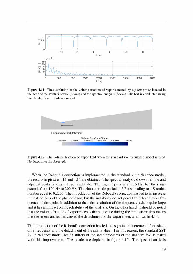
10 20 30 40 50 60

0

0.1

0 500 1000 1500 2000 2500 3000 3500 4000

2

4

6

8

10

12

10-3

Figure 4.11: Time evolution of the volume fraction of vapor detected by a point probe located inthe neck of the Venturi nozzle (above) and the spectral analysis (below). The test is conducted usingthe standard k-ε turbulence model.

Fluctuation without detachment

Figure 4.12: The volume fraction of vapor field when the standard k-ε turbulence model is used.No detachment is observed.

When the Reboud’s correction is implemented in the standard k-ε turbulence model,the results in picture 4.13 and 4.14 are obtained. The spectral analysis shows multiple andadjacent peaks having a large amplitude. The highest peak is at 176 Hz, but the rangeextends from 150 Hz to 200 Hz. The characteristic period is 5.7 ms, leading to a Strouhalnumber equal to 0.2205. The introduction of the Reboud’s correction has led to an increasein unsteadiness of the phenomenon, but the instability do not permit to detect a clear fre-quency of the cycle. In addition to that, the resolution of the frequency axis is quite largeand it has an impact on the reliability of the analysis. On the other hand, it should be notedthat the volume fraction of vapor reaches the null value during the simulation; this meansthat the re-entrant jet has caused the detachment of the vapor sheet, as shown in 4.14.

The introduction of the Reboud’s correction has led to a significant increment of the shed-ding frequency and the detachment of the cavity sheet. For this reason, the standard SSTk-ω turbulence model, which suffers of the same problems of the standard k-ε, is testedwith this improvement. The results are depicted in figure 4.15. The spectral analysis

49

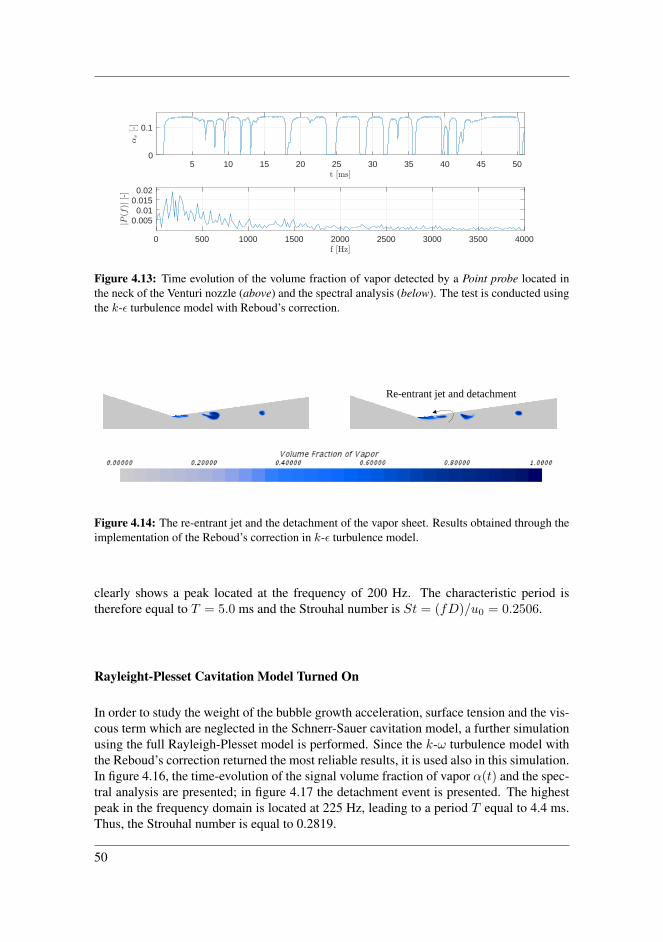
5 10 15 20 25 30 35 40 45 50

0

0.1

0 500 1000 1500 2000 2500 3000 3500 4000

0.005

0.01

0.015

0.02

Figure 4.13: Time evolution of the volume fraction of vapor detected by a Point probe located inthe neck of the Venturi nozzle (above) and the spectral analysis (below). The test is conducted usingthe k-ε turbulence model with Reboud’s correction.

Re-entrant jet and detachment

Figure 4.14: The re-entrant jet and the detachment of the vapor sheet. Results obtained through theimplementation of the Reboud’s correction in k-ε turbulence model.

clearly shows a peak located at the frequency of 200 Hz. The characteristic period istherefore equal to T = 5.0 ms and the Strouhal number is St = (fD)/u0 = 0.2506.

Rayleight-Plesset Cavitation Model Turned On

In order to study the weight of the bubble growth acceleration, surface tension and the vis-cous term which are neglected in the Schnerr-Sauer cavitation model, a further simulationusing the full Rayleigh-Plesset model is performed. Since the k-ω turbulence model withthe Reboud’s correction returned the most reliable results, it is used also in this simulation.In figure 4.16, the time-evolution of the signal volume fraction of vapor α(t) and the spec-tral analysis are presented; in figure 4.17 the detachment event is presented. The highestpeak in the frequency domain is located at 225 Hz, leading to a period T equal to 4.4 ms.Thus, the Strouhal number is equal to 0.2819.

50

10 20 30 40 50 60 70 80

0

0.1

0 500 1000 1500 2000 2500 3000 3500 4000

0.02

0.04

Figure 4.15: Time evolution of the volume fraction of vapor detected by a point probe located inthe neck of the Venturi nozzle (above) and the spectral analysis (below). The test is conducted usingthe k-ω turbulence model with the Reboud’s correction.

10 20 30 40 50 60 70 80

0

0.1

0 500 1000 1500 2000 2500 3000 3500 4000

0.005

0.01

0.015

0.02

Figure 4.16: Time evolution of the volume fraction of vapor detected by a Point probe located in theneck of the Venturi nozzle (above) and the spectral analysis of the signal (below). The test is con-ducted using the k-ω turbulent model with Reboud’s correction and full Rayleigh-Plesset cavitationmodel.

Figure 4.17: Detachment of the vapor bubble with the Rayleigh-Plesset cavitation model, Reboud’scorrection and k − ε turbulence model.

51

4.1.8 DiscussionBefore discussing in details the numerical results, they are summarized in table 4.3. Again,all the results are obtained with the seed density and seed diameter equal to 1011 m−3

and 5 µm.

Frequency [Hz] Strouhal Relative Error [-]

Schnerr-SauerStandard k − ε 104 0.1303 44%k − ε Reboud 176 0.2205 7%k − ω Reboud 200 0.2506 6%

Rayleigh-Plesset k − ω Reboud 225 0.2819 17 %Experimental values 188.6 0.2319 -

Table 4.3: Summary of my numerical results and the experimental values by Jahangir et al. [28].

As it might be noted, the turbulence model has a large impact on the solution; this wasexpected from the analysis by Coutier-Delgosha et al. [17]. In particular, as shown bythe authors, due to the high value of the turbulence viscosity close to the cavitation sheet,the re-entrant jet is not able to reach the throat and cause the detachment. This situationmight be seen, for instance, in figure 4.11, where the point probe always detects a volumefraction of vapor. In addition, when the standard k-ε is used, the frequency is underesti-mated, despite the signal shows a nice periodic behaviour. The relative error is, indeed,large, εr = 44%.

With the aim of decreasing the eddy viscosity close to the cavitation sheet and increasingthe shedding frequency, the Rebound’s correction is introduced in k-ε turbulence model.This leads to an increase of 69% of the shedding frequency. Moreover, in this case, thetime evolution of the signal shows that the volume fraction of vapor reaches the zero,meaning that the re-entrant stream could arrive at the neck of the Venturi. However, inthe spectral analysis, there is a complex time-evolution of the signal, since multiple peaksaround 176 Hz are observed. The range is approximately from 150 Hz to 350 Hz.

Because of the reliability of the SST k-ω turbulence model in case of adverse pressuregradients, the Reboud’s modified version of the SST k-ω model is tested. In this case,only one and evident peak is observed in the spectral analysis; it is at 200 Hz. It is closeto the experimental data, being the relative error equal to 6%. This value, that at the firstglance might appear quite large, is acceptable considering the assumption used in the sim-ulation. The axisymmetry, the use of the URANS equations, the VOF method and thecavitation model introduce, unavoidably, errors. From picture 4.18, the dynamics of thecavitation bubbles shows a satisfying agreement with the actual physics. In this picture,the volume fraction of vapour is depicted in the region of interest. The time developmentis described using the non dimensional time t∗ = t/T , where T is the shedding period.

The re-entrant jet is observed in the break-off cycle only when the Reboud’s correc-tion is implemented. A representation of the velocity field is presented in figure 4.19,zooming on the area of interest for the time-step t∗ = 0.24. In order to detect the velocity

52

(a) t∗ = 0

(b) t∗ = 0.24

(c) t∗ = 0.29

(d) t∗ = 0.41

(e) t∗ = 0.78

(f) t∗ = 1

Figure 4.18: The break off cycle obtained using the SST k−ω turbulence model with the Reboud’scorrection

53

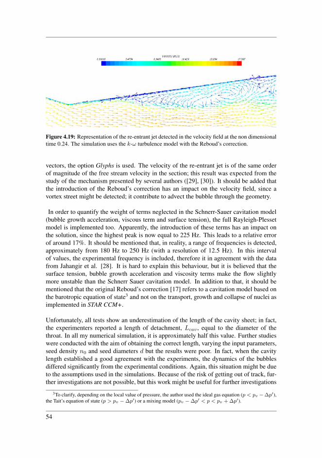
Figure 4.19: Representation of the re-entrant jet detected in the velocity field at the non dimensionaltime 0.24. The simulation uses the k-ω turbulence model with the Reboud’s correction.

vectors, the option Glyphs is used. The velocity of the re-entrant jet is of the same orderof magnitude of the free stream velocity in the section; this result was expected from thestudy of the mechanism presented by several authors ([29], [30]). It should be added thatthe introduction of the Reboud’s correction has an impact on the velocity field, since avortex street might be detected; it contribute to advect the bubble through the geometry.

In order to quantify the weight of terms neglected in the Schnerr-Sauer cavitation model(bubble growth acceleration, viscous term and surface tension), the full Rayleigh-Plessetmodel is implemented too. Apparently, the introduction of these terms has an impact onthe solution, since the highest peak is now equal to 225 Hz. This leads to a relative errorof around 17%. It should be mentioned that, in reality, a range of frequencies is detected,approximately from 180 Hz to 250 Hz (with a resolution of 12.5 Hz). In this intervalof values, the experimental frequency is included, therefore it in agreement with the datafrom Jahangir et al. [28]. It is hard to explain this behaviour, but it is believed that thesurface tension, bubble growth acceleration and viscosity terms make the flow slightlymore unstable than the Schnerr Sauer cavitation model. In addition to that, it should bementioned that the original Reboud’s correction [17] refers to a cavitation model based onthe barotropic equation of state3 and not on the transport, growth and collapse of nuclei asimplemented in STAR CCM+.

Unfortunately, all tests show an underestimation of the length of the cavity sheet; in fact,the experimenters reported a length of detachment, Lcav , equal to the diameter of thethroat. In all my numerical simulation, it is approximately half this value. Further studieswere conducted with the aim of obtaining the correct length, varying the input parameters,seed density n0 and seed diameters d but the results were poor. In fact, when the cavitylength established a good agreement with the experiments, the dynamics of the bubblesdiffered significantly from the experimental conditions. Again, this situation might be dueto the assumptions used in the simulations. Because of the risk of getting out of track, fur-ther investigations are not possible, but this work might be useful for further investigations

3To clarify, depending on the local value of pressure, the author used the ideal gas equation (p < pv −∆p′),the Tait’s equation of state (p > pv − ∆p′) or a mixing model (pv − ∆p′ < p < pv + ∆p′).

54

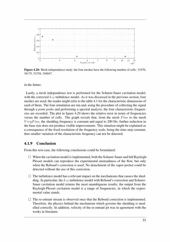
3 4 5 6 7 8 9 10 11 12

104

0

0.2

0.4

0.6

0.8

1

Figure 4.20: Mesh independence study; the four meshes have the following number of cells: 31070,36175, 51538, 104847.

in the future.

Lastly, a mesh independence test is performed for the Schnerr-Sauer cavitation model,with the corrected k-ω turbulence model. As it was discussed in the previous section, fourmeshes are used; the reader might refer to the table 4.1 for the characteristic dimensions ofeach of them. The four simulation are run and, using the procedure of collecting the signalthrough a point probe and performing a spectral analysis, the four characteristic frequen-cies are recorded. The plot in figure 4.20 shows the relative error in terms of frequenciesversus the number of cells. The graph reveals that, from the mesh Fine to the meshV eryF ine, the shedding frequency is constant and equal to 200 Hz; further reduction inthe base size does not produce visible improvements. This situation might be explained asa consequence of the fixed resolution of the frequency scale, being the time-step constant,thus smaller variation of the characteristic frequency can not be detected.

4.1.9 ConclusionFrom this test-case, the following conclusions could be formulated:

When the cavitation model is implemented, both the Schnerr-Sauer and full Rayleigh-Plesset models can reproduce the experimental unsteadiness of the flow, but onlywhen the Reboud’s correction is used. No detachment of the vapor pocket could bedetected without the use of this correction.

The turbulence model has a relevant impact on the mechanisms that causes the shed-ding. In particular, the k-ω turbulence model with Reboud’s correction and Schnerr-Sauer cavitation model returns the most unambiguous results; the output from theRayleigh-Plesset cavitation model is a range of frequencies, in which the experi-mental value stands.

The re-entrant stream is observed once that the Reboud correction is implemented.Therefore, the physics behind the mechanism which governs the shedding is mod-elled correctly. In addition, velocity of the re-entrant jet was in agreement with theworks in literature.

55

The length of detachment is underestimated; this might be due to the combined ef-fect of cavitation model and turbulence model. Further investigation using a differ-ent cavitation model (barotropic law), turbulence model (Large Eddies Simulation)and Eulerian multiphase method should be performed to obtain clear picture.

56

4.2 Single phase flowThe second validation case of this project is about the single phase flow in the nozzles ofthe injector when the cut-off shaft is moving. It allows to gain confidence with the over-set technique and make a preliminary analysis of the effects of the motion of the cut-offshaft. Because of the lack of experimental records, the numerical values will be comparedwith the data from the one dimensional code 1D-Hydcode, internally developed by MANEnergy Solutions. 1D-Hydcode implements the one dimensional Navier-Stokes equationand it considers the entire injection system, from the high pressure line to the nozzle holes.In addition, the outputs of this tool (needle lift and pressure in the boundaries) are imple-mented as inputs for the CFD simulation. This procedure allows a cross validation of thetwo numerical models. The injection event lasts approximately 30 ms and, due to the smalltime-step required by the simulations (in the order of micro-seconds), the start of injection(SOI) and the end of injection (EOI) will be studied independently.

Similarly to the previous chapter, this section is organized following the workflow ofSTAR CCM+: the geometry, physics, boundary condition, mesh and solvers are presented.The results are shown and commented in the following two sections.

4.2.1 GeometryThe CAD geometry of the injector is provided by Simon Matlok, research engineer ofMAN Energy Solutions. This project is not aimed at simulating the flow in the entire in-jection system because of the dimensions of the components (recall, for instance, that onlythe high pressure pipe has a length of 1.9 m) and their complexity. For this reason, onlythree components of the injector valve located beneath the spring (refer to section 2.9 toremind the injection system) are considered. They are named spindle guide, spindle andfuel nozzle and they are depicted in figure 4.21, 4.22 and 4.23 respectively.

The fuel nozzle is characterized by four orifices with a diameter of 1.05 mm. The nozzleholes are not tapered, meaning that the inlet diameter has the same dimension of the out-let diameter. In other words, the k-factor is equal to 0. As reported in the Introduction,in the State of Art section, this condition is favorable to cavitation. In fact, the sectionarea decreases abruptly from the sac to the orifices and the same happens for the pressure,which could potentially drop under the saturation limit. With the aim of avoiding a tumul-tuous cavitation regime and its consequences in terms of erosion, the engineers designedspherical smooth entrance in two nozzle holes with a radius of 1.2 mm; in this way, theCarnot-Borda pressure losses are minimized. Lastly, the ratio between the length and theoutlet diameter (L/Do) is equal to 3 and 3.8 respectively for the two central and externalholes. From this paragraph, the nozzle holes will be identified with the following notation,H1, H2, H3 and H4, as depicted in figure 4.23.

The CAD geometry is provided with some corrections to avoid problems due to smallgeometrical features and crevices. It is further simplified cutting off most of the upstreampart of the spindle guide and spindle. In this way, the internal surface of the spindle guideand the external surface of the spindle are always in contact. In figure 4.24, a comparison

57

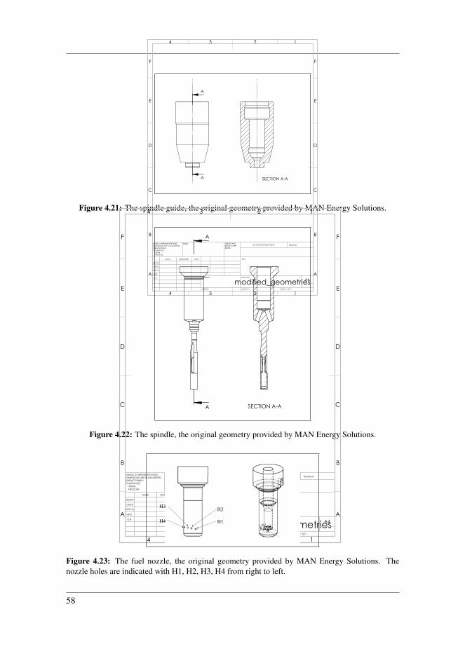
A

A SECTION A-A

A A

B B

C C

D D

E E

F F

4

4

3

3

2

2

1

1

DRAWN

CHK'D

APPV'D

MFG

Q.A

UNLESS OTHERWISE SPECIFIED:DIMENSIONS ARE IN MILLIMETERSSURFACE FINISH:TOLERANCES: LINEAR: ANGULAR:

FINISH: DEBURR AND BREAK SHARP EDGES

NAME SIGNATURE DATE

MATERIAL:

DO NOT SCALE DRAWING REVISION

TITLE:

DWG NO.

SCALE:1:1 SHEET 1 OF 1

A4

WEIGHT:

modified_geometries

Figure 4.21: The spindle guide, the original geometry provided by MAN Energy Solutions.

A

A SECTION A-A

A A

B B

C C

D D

E E

F F

4

4

3

3

2

2

1

1

DRAWN

CHK'D

APPV'D

MFG

Q.A

UNLESS OTHERWISE SPECIFIED:DIMENSIONS ARE IN MILLIMETERSSURFACE FINISH:TOLERANCES: LINEAR: ANGULAR:

FINISH: DEBURR AND BREAK SHARP EDGES

NAME SIGNATURE DATE

MATERIAL:

DO NOT SCALE DRAWING REVISION

TITLE:

DWG NO.

SCALE:1:1 SHEET 1 OF 1

A4

WEIGHT:

modified_geometries

Figure 4.22: The spindle, the original geometry provided by MAN Energy Solutions.

H2

H1 H4

H3

Figure 4.23: The fuel nozzle, the original geometry provided by MAN Energy Solutions. Thenozzle holes are indicated with H1, H2, H3, H4 from right to left.

58

Figure 4.24: The original geometry of the assembly (Left) and its modified version (Right).

between the original assembly and the updated version is presented. Lastly, by means ofthe Surface Repair Tool integrated in the software, the inlet and outlet surfaces are defined.

Applying the Outlet pressure boundary condition directly on outlet surfaces (H1, H2,H3 and H4) might cause unrealistic flow and it might lead to divergence because it couldinfluence the flow upstream. For this reason, as suggested by Gavaises et al. [21] and An-dersen [5], expansion volumes of conical shape are created in CAD software (Solidworks,as Loft volumes) and imported in STAR CCM+. Special attention was given in the place-ment of the expansion volumes in the outlet surface of the nozzle holes. The geometrywith the expansion volumes is presented in figure 4.25. In this picture, the fuel valve iscompletely open and the expansion volumes are depicted in orange. The inlet boundary iscoloured in purple.

59

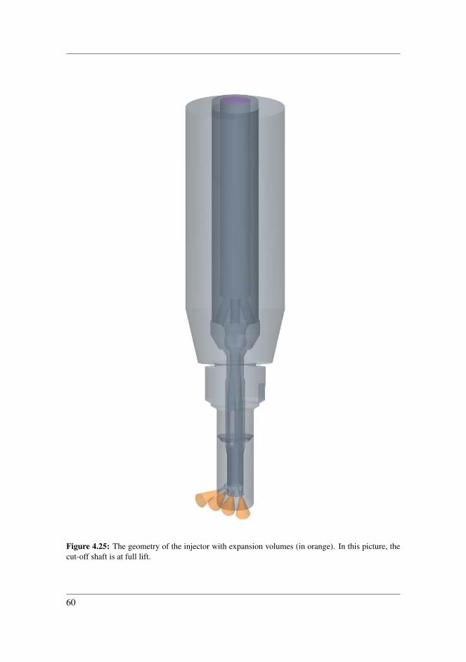
Figure 4.25: The geometry of the injector with expansion volumes (in orange). In this picture, thecut-off shaft is at full lift.

60

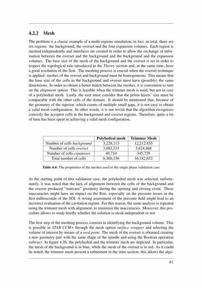
4.2.2 Mesh

The problem is a classic example of a multi-regions simulation; in fact, in total, there aresix regions: the background, the overset and the four expansion volumes. Each region ismeshed independently and interfaces are created in order to allow the exchange of infor-mation between the overset and the background and the background and the expansionvolumes. The base size of the mesh of the background and the overset is set in order torespect the topological rule introduced in the Theory section and, at the same time, havea good resolution of the flow. The meshing process is crucial when the overset techniqueis applied: meshes of the overset and background must be homogeneous. This means thatthe base size of the cells in the background and overset must have (possibly) the samedimensions. In order to obtain a better match between the meshes, it is convenient to turnon the alignment option. This is feasible when the trimmer mesh is used, but not in caseof a polyhedral mesh. Lastly, the user must consider that the prism layers’ size must becomparable with the other cells of the domain. It should be mentioned that, because ofthe geometry of the injector, which counts of multiple small gaps, it is not easy to obtaina valid mesh configuration. In other words, it is not trivial that the algorithm recognizescorrectly the acceptor cells in the background and overset regions. Therefore, quite a lotof time has been spent in achieving a valid mesh configuration.

Polyhedral mesh Trimmer MeshNumber of cells background 3,228,113 12,212,455

Number of cells overset 3,082,333 3,624,468Number of cells expansors 49,710 345,729

Total number of cells 6,360,156 16,182,652

Table 4.4: The proprieties of the meshes used in the single phase validation case

At the starting point of this validation case, the polyhedral mesh was selected; unfortu-nately, it was noted that the lack of alignment between the cells of the background andthe overset produced ”staircase” geometry during the opening and closing event. Theseinaccuracies might have an impact on the flow, especially on the pressure losses in thefirst milliseconds of the SOI. A wrong assessment of the pressure field might lead to anincorrect evaluation of the cavitation regime. For this reason, the same analysis is repeatedusing the trimmer mesh with alignment, to minimize the inaccuracies. Moreover, this pro-cedure allows to study briefly whether the solution is mesh independent or not.

The first step of the meshing process consists in identifying the background volume. Thisis possible in STAR CCM+ through the mesh option surface wrapper and selecting thevolume of interest by means of a seed point. The mesh of the overset is obtained creatinga new geometry part with the same shape of the spindle and using the Boolean operationsubtract. In figure 4.26, the polyhedral and the trimmer mesh are depicted. In particular,the mesh of the background is in blue, while the mesh of the overset is in red. As it couldbe noted, the trimmer mesh present a refinement in the inlet section; this allows the algo-

61

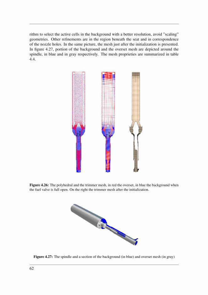
rithm to select the active cells in the background with a better resolution, avoid ”scaling”geometries. Other refinements are in the region beneath the seat and in correspondenceof the nozzle holes. In the same picture, the mesh just after the initialization is presented.In figure 4.27, portion of the background and the overset mesh are depicted around thespindle, in blue and in gray respectively. The mesh proprieties are summarized in table4.4.

Figure 4.26: The polyhedral and the trimmer mesh, in red the overset, in blue the background whenthe fuel valve is full open. On the right the trimmer mesh after the initialization.

Figure 4.27: The spindle and a section of the background (in blue) and overset mesh (in gray)

62

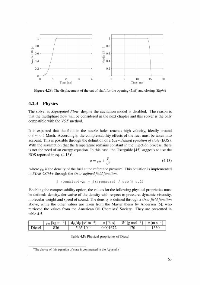
0 1 2 3 4

0

0.2

0.4

0.6

0.8

1

0 5 10 15 20

0

0.2

0.4

0.6

0.8

1

Figure 4.28: The displacement of the cut of shaft for the opening (Left) and closing (Right)

4.2.3 PhysicsThe solver is Segregated Flow, despite the cavitation model is disabled. The reason isthat the multiphase flow will be considered in the next chapter and this solver is the onlycompatible with the VOF method.

It is expected that the fluid in the nozzle holes reaches high velocity, ideally around0.3 ∼ 0.4 Mach. Accordingly, the compressability effects of the fuel must be taken intoaccount. This is possible through the definition of a User-defined equation of state (EOS).With the assumption that the temperature remains constant in the injection process, thereis not the need of an energy equation. In this case, the Userguide [45] suggests to use theEOS reported in eq. (4.13)4:

ρ = ρ0 +p

c2(4.13)

where ρ0 is the density of the fuel at the reference pressure. This equation is implementedin STAR CCM+ through the User-defined field function:

$ (Density)=ρ0 + $(Pressure) / pow($ c,2)

Enabling the compressability option, the values for the following physical proprieties mustbe defined: density, derivative of the density with respect to pressure, dynamic viscosity,molecular weight and speed of sound. The density is defined through a User field functionabove, while the other values are taken from the Master thesis by Andersen [5], whoretrieved the values from the American Oil Chemists’ Society. They are presented intable 4.5.

ρ0 [kg m−3] dρ/dp [s2 m−2] µ [Pa s] W [g mol−1] c [m s−1]Diesel 836 5.65 10−7 0.001672 170 1330

Table 4.5: Physical proprieties of Diesel

4The choice of this equation of state is commented in the Appendix

63

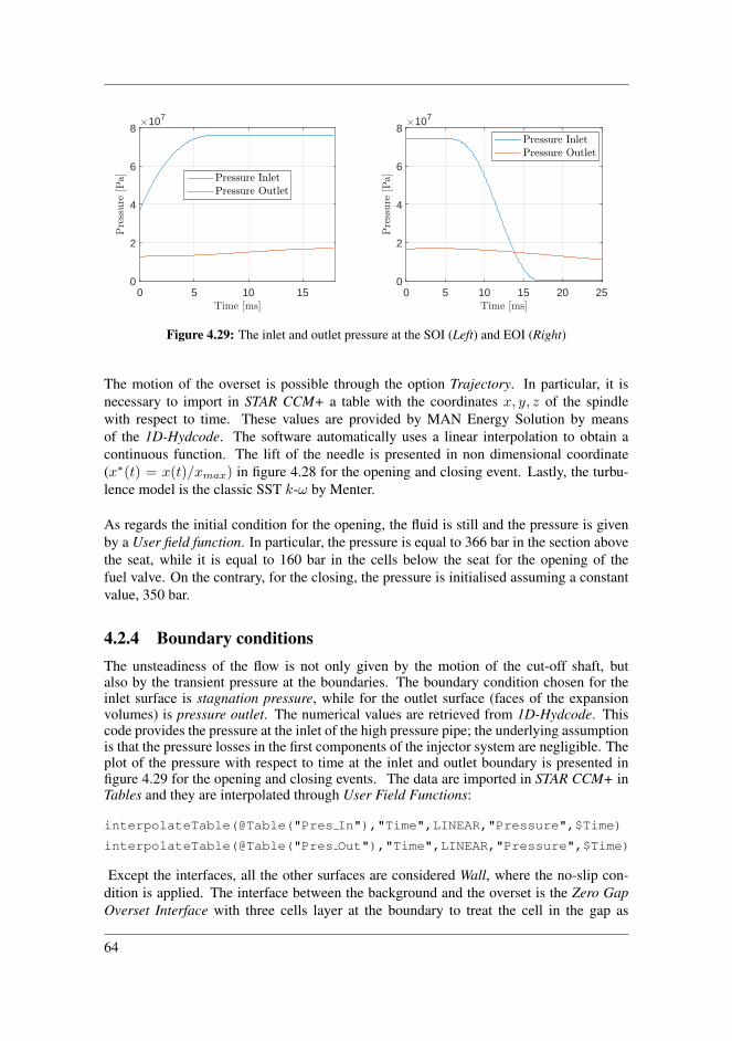
0 5 10 15

0

2

4

6

810

7

0 5 10 15 20 25

0

2

4

6

810

7

Figure 4.29: The inlet and outlet pressure at the SOI (Left) and EOI (Right)

The motion of the overset is possible through the option Trajectory. In particular, it isnecessary to import in STAR CCM+ a table with the coordinates x, y, z of the spindlewith respect to time. These values are provided by MAN Energy Solution by meansof the 1D-Hydcode. The software automatically uses a linear interpolation to obtain acontinuous function. The lift of the needle is presented in non dimensional coordinate(x∗(t) = x(t)/xmax) in figure 4.28 for the opening and closing event. Lastly, the turbu-lence model is the classic SST k-ω by Menter.

As regards the initial condition for the opening, the fluid is still and the pressure is givenby a User field function. In particular, the pressure is equal to 366 bar in the section abovethe seat, while it is equal to 160 bar in the cells below the seat for the opening of thefuel valve. On the contrary, for the closing, the pressure is initialised assuming a constantvalue, 350 bar.

4.2.4 Boundary conditionsThe unsteadiness of the flow is not only given by the motion of the cut-off shaft, butalso by the transient pressure at the boundaries. The boundary condition chosen for theinlet surface is stagnation pressure, while for the outlet surface (faces of the expansionvolumes) is pressure outlet. The numerical values are retrieved from 1D-Hydcode. Thiscode provides the pressure at the inlet of the high pressure pipe; the underlying assumptionis that the pressure losses in the first components of the injector system are negligible. Theplot of the pressure with respect to time at the inlet and outlet boundary is presented infigure 4.29 for the opening and closing events. The data are imported in STAR CCM+ inTables and they are interpolated through User Field Functions:

interpolateTable(@Table("Pres In"),"Time",LINEAR,"Pressure",$Time)

interpolateTable(@Table("Pres Out"),"Time",LINEAR,"Pressure",$Time)

Except the interfaces, all the other surfaces are considered Wall, where the no-slip con-dition is applied. The interface between the background and the overset is the Zero GapOverset Interface with three cells layer at the boundary to treat the cell in the gap as

64

inactive, while the interfaces between the background and the expansors are Internal In-terfaces.

4.2.5 SolverThe solver is Segregated Flow and the time discretization is Euler Second Order. The timestep is changed during the simulation in order to have a trade-off between the time requiredto obtain a solution (the simulations are very CPU intensive) and the Courant number. Inparticular, the first milliseconds of the opening event were simulated considering a timestep equal to 1 µs (Courant less than 15 in all the cells of the domain), and it was increaseduntil 5µ in the further time interval.The inner number of iteration is equal to 5; this value is chosen since it is observed that,for this value, the time derivative of the residuals is small enough. In the simulations,the default values for the under-relaxation factors need to be slightly decreased to avoiddivergence. The option Linear ramp has been used both for the turbulence model andpressure solver.

4.2.6 ResultsThis section is aimed at presenting the most relevant results of the simulations. Let us startconsidering the start of injection event (the opening of the fuel valve); the end of injectionevent (the closing of the fuel valve) is reported in the following subsection.

The Start of Injection

The first parameter which deserves special attention is the mass flow. In fact, on theengineering point of view, it essential to know the amount of fuel diesel injected in thecombustion chamber, in order to predict correctly the stoichiometric ratio air/fuel and,consequently, the performance of the engine. The mass flow per each of the four holes ofthe injector is calculated using eq. (4.14) and the pre-built functions in STAR CCM+:∫

AHi

ρ(u · n)dA (4.14)

The results in terms of the mass flows through each of the holes of the injector are de-picted in figure 4.30 and 4.31 for the polyhedral and trimmer meshes. Additionally, thetotal mass flow is calculated and plotted in figure 4.32, where the benchmark values fromthe 1D-Hydcode are reported too. It is important to underline that, in the one dimensionalcode used as reference, the displacement of the spindle is the result of the forces actingon it. On the contrary, the motion of the spindle is prescribed in the numerical simulation;in other words, the output of 1D-Hydcode is used as an input in the CFD model. Thishas a large implication on the results which will be commented in the Discussion section.Lastly, it should be mentioned that the 50% of the displacement of the needle does notcause the uncovering of the nozzle holes, this is the reason why a time-span of around1 ms is needed to allow the flow.

65

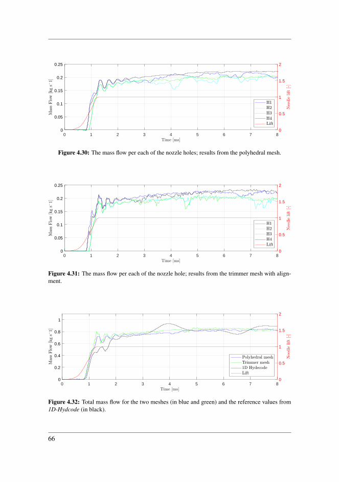
0 1 2 3 4 5 6 7 8

0

0.05

0.1

0.15

0.2

0.25

0

0.5

1

1.5

2

Figure 4.30: The mass flow per each of the nozzle holes; results from the polyhedral mesh.

0 1 2 3 4 5 6 7 8

0

0.05

0.1

0.15

0.2

0.25

0

0.5

1

1.5

2

Figure 4.31: The mass flow per each of the nozzle hole; results from the trimmer mesh with align-ment.

0 1 2 3 4 5 6 7 8

0

0.2

0.4

0.6

0.8

1

0

0.5

1

1.5

2

Figure 4.32: Total mass flow for the two meshes (in blue and green) and the reference values from1D-Hydcode (in black).

66

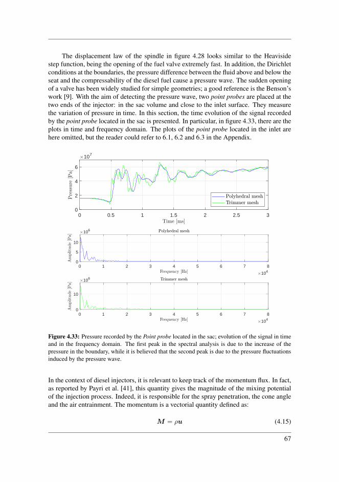
The displacement law of the spindle in figure 4.28 looks similar to the Heavisidestep function, being the opening of the fuel valve extremely fast. In addition, the Dirichletconditions at the boundaries, the pressure difference between the fluid above and below theseat and the compressability of the diesel fuel cause a pressure wave. The sudden openingof a valve has been widely studied for simple geometries; a good reference is the Benson’swork [9]. With the aim of detecting the pressure wave, two point probes are placed at thetwo ends of the injector: in the sac volume and close to the inlet surface. They measurethe variation of pressure in time. In this section, the time evolution of the signal recordedby the point probe located in the sac is presented. In particular, in figure 4.33, there are theplots in time and frequency domain. The plots of the point probe located in the inlet arehere omitted, but the reader could refer to 6.1, 6.2 and 6.3 in the Appendix.

0 0.5 1 1.5 2 2.5 3

0

2

4

6

107

0 1 2 3 4 5 6 7 8

104

0

5

10

106

0 1 2 3 4 5 6 7 8

104

0

10

106

Figure 4.33: Pressure recorded by the Point probe located in the sac; evolution of the signal in timeand in the frequency domain. The first peak in the spectral analysis is due to the increase of thepressure in the boundary, while it is believed that the second peak is due to the pressure fluctuationsinduced by the pressure wave.

In the context of diesel injectors, it is relevant to keep track of the momentum flux. In fact,as reported by Payri et al. [41], this quantity gives the magnitude of the mixing potentialof the injection process. Indeed, it is responsible for the spray penetration, the cone angleand the air entrainment. The momentum is a vectorial quantity defined as:

M = ρu (4.15)

67

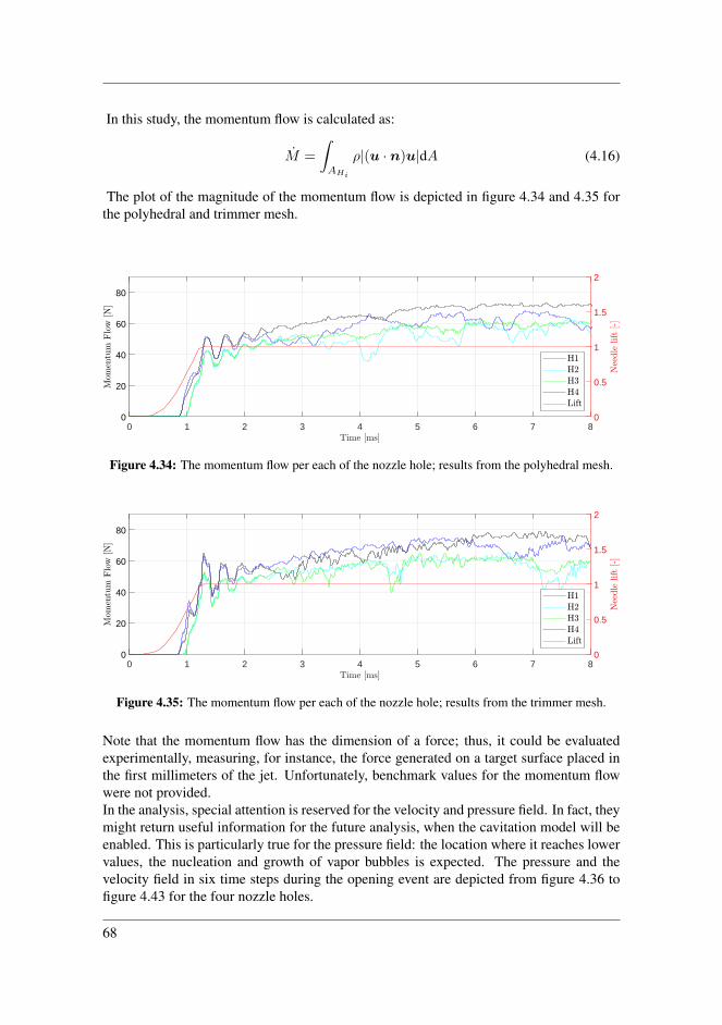
In this study, the momentum flow is calculated as:

M =

∫AHi

ρ|(u · n)u|dA (4.16)

The plot of the magnitude of the momentum flow is depicted in figure 4.34 and 4.35 forthe polyhedral and trimmer mesh.

0 1 2 3 4 5 6 7 8

0

20

40

60

80

0

0.5

1

1.5

2

Figure 4.34: The momentum flow per each of the nozzle hole; results from the polyhedral mesh.

0 1 2 3 4 5 6 7 8

0

20

40

60

80

0

0.5

1

1.5

2

Figure 4.35: The momentum flow per each of the nozzle hole; results from the trimmer mesh.

Note that the momentum flow has the dimension of a force; thus, it could be evaluatedexperimentally, measuring, for instance, the force generated on a target surface placed inthe first millimeters of the jet. Unfortunately, benchmark values for the momentum flowwere not provided.In the analysis, special attention is reserved for the velocity and pressure field. In fact, theymight return useful information for the future analysis, when the cavitation model will beenabled. This is particularly true for the pressure field: the location where it reaches lowervalues, the nucleation and growth of vapor bubbles is expected. The pressure and thevelocity field in six time steps during the opening event are depicted from figure 4.36 tofigure 4.43 for the four nozzle holes.

68

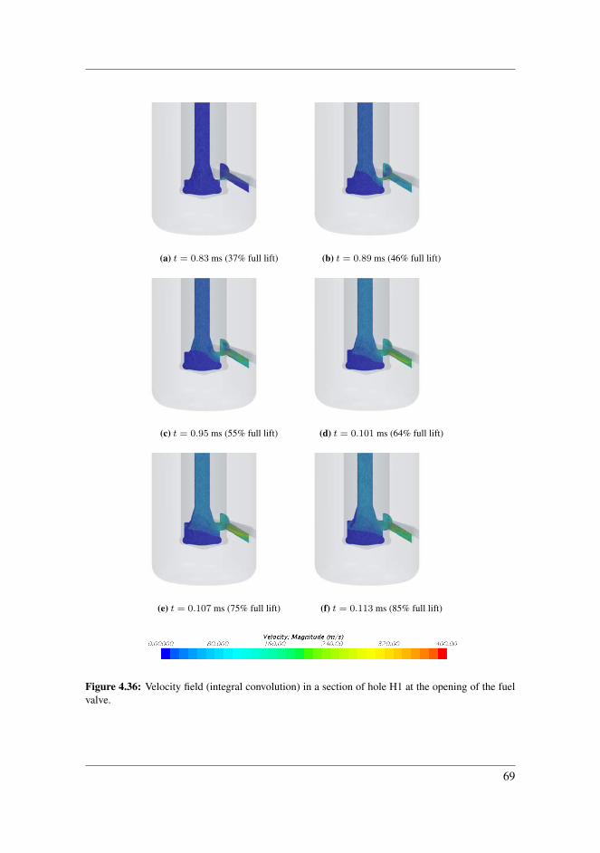
(a) t = 0.83 ms (37% full lift) (b) t = 0.89 ms (46% full lift)

(c) t = 0.95 ms (55% full lift) (d) t = 0.101 ms (64% full lift)

(e) t = 0.107 ms (75% full lift) (f) t = 0.113 ms (85% full lift)

Figure 4.36: Velocity field (integral convolution) in a section of hole H1 at the opening of the fuelvalve.

69

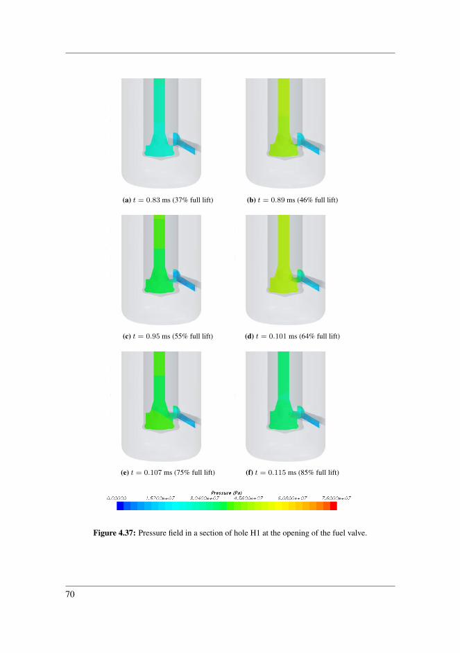
(a) t = 0.83 ms (37% full lift) (b) t = 0.89 ms (46% full lift)

(c) t = 0.95 ms (55% full lift) (d) t = 0.101 ms (64% full lift)

(e) t = 0.107 ms (75% full lift) (f) t = 0.115 ms (85% full lift)

Figure 4.37: Pressure field in a section of hole H1 at the opening of the fuel valve.

70

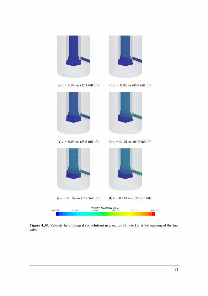
(a) t = 0.83 ms (37% full lift) (b) t = 0.89 ms (46% full lift)

(c) t = 0.95 ms (55% full lift) (d) t = 0.101 ms (64% full lift)

(e) t = 0.107 ms (75% full lift) (f) t = 0.113 ms (85% full lift)

Figure 4.38: Velocity field (integral convolution) in a section of hole H2 at the opening of the fuelvalve

71

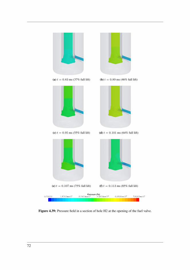
(a) t = 0.83 ms (37% full lift) (b) t = 0.89 ms (46% full lift)

(c) t = 0.95 ms (55% full lift) (d) t = 0.101 ms (64% full lift)

(e) t = 0.107 ms (75% full lift) (f) t = 0.113 ms (85% full lift)

Figure 4.39: Pressure field in a section of hole H2 at the opening of the fuel valve.

72

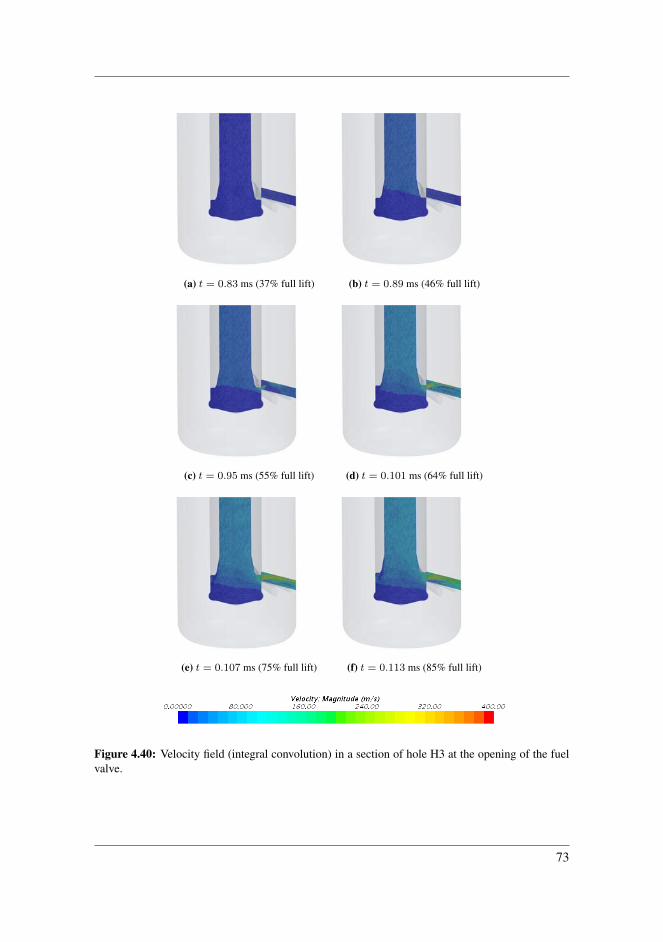
(a) t = 0.83 ms (37% full lift) (b) t = 0.89 ms (46% full lift)

(c) t = 0.95 ms (55% full lift) (d) t = 0.101 ms (64% full lift)

(e) t = 0.107 ms (75% full lift) (f) t = 0.113 ms (85% full lift)

Figure 4.40: Velocity field (integral convolution) in a section of hole H3 at the opening of the fuelvalve.

73

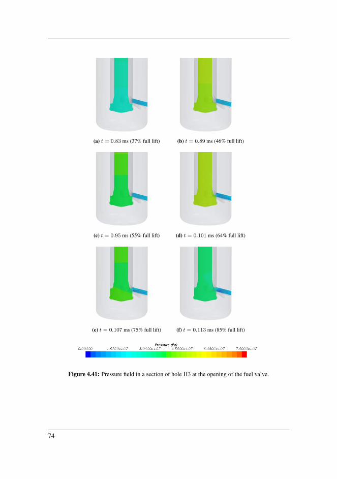
(a) t = 0.83 ms (37% full lift) (b) t = 0.89 ms (46% full lift)

(c) t = 0.95 ms (55% full lift) (d) t = 0.101 ms (64% full lift)

(e) t = 0.107 ms (75% full lift) (f) t = 0.113 ms (85% full lift)

Figure 4.41: Pressure field in a section of hole H3 at the opening of the fuel valve.

74

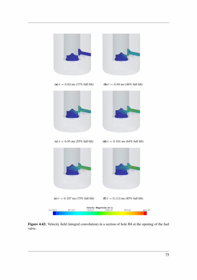
(a) t = 0.83 ms (37% full lift) (b) t = 0.89 ms (46% full lift)

(c) t = 0.95 ms (55% full lift) (d) t = 0.101 ms (64% full lift)

(e) t = 0.107 ms (75% full lift) (f) t = 0.113 ms (85% full lift)

Figure 4.42: Velocity field (integral convolution) in a section of hole H4 at the opening of the fuelvalve.

75

(a) t = 0.83 ms (37% full lift) (b) t = 0.89 ms (46% full lift)

(c) t = 0.95 ms (55% full lift) (d) t = 0.101 ms (64% full lift)

(e) t = 0.107 ms (75% full lift) (f) t = 0.113 ms (85% full lift)

Figure 4.43: Pressure field in a section of hole H4 at the opening of the fuel valve. It is interestingto note a large vortex which is generated at the entrance of the nozzle hole.

76

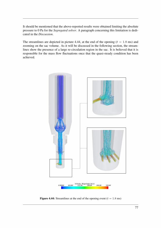
It should be mentioned that the above-reported results were obtained limiting the absolutepressure to 0 Pa for the Segregated solver. A paragraph concerning this limitation is dedi-cated in the Discussion.

The streamlines are depicted in picture 4.44, at the end of the opening (t = 1.8 ms) andzooming on the sac volume. As it will be discussed in the following section, the stream-lines show the presence of a large re-circulation region in the sac. It is believed that it isresponsible for the mass flow fluctuations once that the quasi-steady condition has beenachieved.

Figure 4.44: Streamlines at the end of the opening event (t = 1.8 ms)

77

The End of Injection

The study of the end of injection is performed using the polyhedral and trimmer mesh, in asimilar way of what has been done for the start of injection. The EOI differs from the SOIbecause it is necessary to reach the quasi-steady condition before the cut-off shaft starts itsmotion. For this reason, in the first 13 ms the valve is at full lift and the flow has time todevelop and evolve due to the time dependant pressure at the boundaries. The mass flowthrough the orifices is reported in figure 4.45 and 4.46, respectively for the polyhedral andthe trimmer mesh. In figure 4.47, the total mass flow is calculated and it is compared withthe data from the 1D-Hydcode. The plots of the momentum flow are here omitted, but thereader could refer to the Appendix.

The reader might note that, at time-step 14 ms, the flow reverse; the mass flows through thefour nozzle holes change sign and become negative. It is the moment when the pressureat the inlet starts to be lower than the pressure at the outlet (refer to figure 4.29). Negativemass flows are not realistic and they might be caused by the misalignment between thehypotheses of the CFD simulation and the 1D-Hydcode, as it will be commented later inthe Discussion subsection.

5 6 7 8 9 10 11 12 13 14 15 16

-0.1

-0.05

0

0.05

0.1

0.15

0.2

0

0.5

1

1.5

2

Figure 4.45: The mass flow per each of the nozzle hole; results from the polyhedral mesh.

4 6 8 10 12 14 16

-0.1

-0.05

0

0.05

0.1

0.15

0.2

0

0.5

1

1.5

2

Figure 4.46: The mass flow per each of the nozzle hole; results from the trimmer mesh.

78

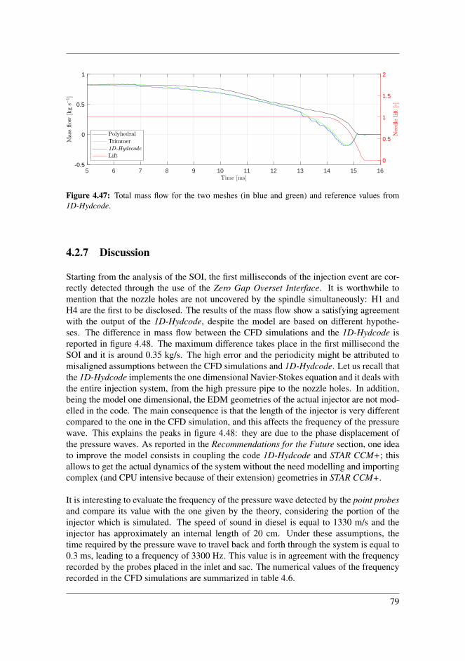
5 6 7 8 9 10 11 12 13 14 15 16

-0.5

0

0.5

1

0

0.5

1

1.5

2

Figure 4.47: Total mass flow for the two meshes (in blue and green) and reference values from1D-Hydcode.

4.2.7 Discussion

Starting from the analysis of the SOI, the first milliseconds of the injection event are cor-rectly detected through the use of the Zero Gap Overset Interface. It is worthwhile tomention that the nozzle holes are not uncovered by the spindle simultaneously: H1 andH4 are the first to be disclosed. The results of the mass flow show a satisfying agreementwith the output of the 1D-Hydcode, despite the model are based on different hypothe-ses. The difference in mass flow between the CFD simulations and the 1D-Hydcode isreported in figure 4.48. The maximum difference takes place in the first millisecond theSOI and it is around 0.35 kg/s. The high error and the periodicity might be attributed tomisaligned assumptions between the CFD simulations and 1D-Hydcode. Let us recall thatthe 1D-Hydcode implements the one dimensional Navier-Stokes equation and it deals withthe entire injection system, from the high pressure pipe to the nozzle holes. In addition,being the model one dimensional, the EDM geometries of the actual injector are not mod-elled in the code. The main consequence is that the length of the injector is very differentcompared to the one in the CFD simulation, and this affects the frequency of the pressurewave. This explains the peaks in figure 4.48: they are due to the phase displacement ofthe pressure waves. As reported in the Recommendations for the Future section, one ideato improve the model consists in coupling the code 1D-Hydcode and STAR CCM+; thisallows to get the actual dynamics of the system without the need modelling and importingcomplex (and CPU intensive because of their extension) geometries in STAR CCM+.

It is interesting to evaluate the frequency of the pressure wave detected by the point probesand compare its value with the one given by the theory, considering the portion of theinjector which is simulated. The speed of sound in diesel is equal to 1330 m/s and theinjector has approximately an internal length of 20 cm. Under these assumptions, thetime required by the pressure wave to travel back and forth through the system is equal to0.3 ms, leading to a frequency of 3300 Hz. This value is in agreement with the frequencyrecorded by the probes placed in the inlet and sac. The numerical values of the frequencyrecorded in the CFD simulations are summarized in table 4.6.

79

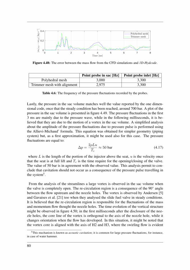
0 1 2 3 4 5 6 7 8

0

0.2

0.4

Figure 4.48: The error between the mass flow from the CFD simulations and 1D-Hydcode.

Point probe in sac [Hz] Point probe inlet [Hz]Polyhedral mesh 3,000 3,300

Trimmer mesh with alignment 2,975 3,300

Table 4.6: The frequency of the pressure fluctuations recorded by the probes.

Lastly, the pressure in the sac volume matches well the value reported by the one dimen-sional code, once that the steady condition has been reached, around 700 bar. A plot of thepressure in the sac volume is presented in figure 4.49. The pressure fluctuations in the first3 ms are mainly due to the pressure wave, while in the following milliseconds, it is be-lieved that they are due to the motion of a vortex in the sac volume. A simplified analysisabout the amplitude of the pressure fluctuations due to pressure pulse is performed usingthe Allievi-Michaud’ formula. This equation was obtained for simpler geometry (pipingsystem) but, as a first approximation, it might be used also for this case. The pressurefluctuations are equal to:

∆p =2ρLu

Tc≈ 50 bar (4.17)

where L is the length of the portion of the injector above the seat, u is the velocity oncethat the seat is at full lift and Tc is the time require for the opening/closing of the valve.The value of 50 bar is in agreement with the observed value. This analysis permit to con-clude that cavitation should not occur as a consequence of the pressure pulse travelling inthe system5.

From the analysis of the streamlines a large vortex is observed in the sac volume whenthe valve is completely open. The re-circulation region is a consequence of the 90 anglebetween the flow upstream and the nozzle holes. The vortex is observed by Andersen [5]and Gavaises et al. [21] too when they analysed the slide fuel valve in steady conditions.It is believed that the re-circulation region is responsible for the fluctuations of the massand momentum flow thought the nozzle holes. The time evolution of the vortical structuremight be observed in figure 4.50; in the first milliseconds after the disclosure of the noz-zle holes, the core line of the vortex is orthogonal to the axis of the nozzle hole, while itchanges orientation when the flow has developed. In this situation, it might be noted thatthe vortex core is aligned with the axis of H2 and H3, where the swirling flow is evident

5This mechanism is known as acoustic cavitation; it is common for large pressure fluctuations, for instance,in case of water hammer.

80

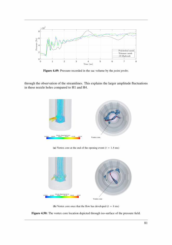
0 1 2 3 4 5 6 7 8

0

2

4

6

8

107

Figure 4.49: Pressure recorded in the sac volume by the point probe.

through the observation of the streamlines. This explains the larger amplitude fluctuationsin these nozzle holes compared to H1 and H4.

Vortex core

(a) Vortex core at the end of the opening event (t = 1.8 ms)

Vortex core

(b) Vortex core once that the flow has developed (t = 8 ms)

Figure 4.50: The vortex core location depicted through iso-surface of the pressure field.

81

From the comparison between the results from the polyhedral and the trimmer mesh, thevariation in pecentage of the mass and momentum flow is small. For instance, the variationin the pressure measured in the sac when the quasi-steady condition is reached is approx-imately equal to 5% on its maximum. This brief analysis allows to demonstrate that thesolution is mesh independent. Regardless that, the trimmer mesh should be preferred inthe following analysis because it is optimized to be used with the overset technology. Infact, the presence of the above mentioned ”scaling” geometries is minimized.

In the project plan of this thesis, a section about the effects of the interpolation optionin the overset was programmed. It was relevant to check the difference in the mass flowdepending on what interpolation scheme is used. Incidentally, on the engineering pointof view, it is essential that the simulation predicts correctly the amount of fuel dischargedby the nozzle holes since it influences the performance of the engine. From a first studyof the Userguide, it seemed that the continuity was automatically fulfilled by the softwarethrough the implementation of corrective algorithm, especially when the Segregated solverwas used. The above mentioned analysis was then pointless. Through further investiga-tion, it was discovered that the mass continuity is enforced only if the user ticks an optionin the Continua window. Unfortunately, the time was too little to perform all the analysesagain, but a quick assessment of the difference is performed. The residuals from the simu-lation run without taking special care of the continuity converges at 10−3, while, enforcingcontinuity, residuals are around 10−6. The error was already very close to be negligible(in general the threshold 10−4 is used in CFD), but, of course, the second solution mustbe preferred. For further studies with the overset and the Segregated solver, it is advisableto enforce the continuity using the Flux correction method, in case of compressible flow.For incompressible flow, the user might choose the Source correction method.

As concern the closing event (EOI), the mass flow from the CFD simulation looks quitedifferent from the benchmark. It might be explained as the consequence of the assump-tions used in the CFD model. In fact, the CFD model uses some of the outputs of the1D-Hydcode, which are based on the 1D Navier-Stokes equation and on a different ge-ometry. In addition to that, it is possible that the 1D-Hydcode does not evaluate correctlythe motion of the cut-off shaft since the three dimensional geometrical features are notreproduced. Being the displacement of the fuel valve prescribed in the CFD simulation,there is an error propagation through the different models.

It should be pointed out that the residual have a magnitude of 10−3 for the continuityand momentum equations. This value is slight larger than the threshold of 10−4 which isoften used to evaluate the convergence of a solution. Anyways, the history of the residualsshows a monotonically decreasing curve, which is perfectly fine. The term responsible forthe production of the turbulent kinetic energy shows this behaviour too. On the contrary,the residuals for the rate of dissipation (abbreviated as Sdr in STAR CCM+) are high (butthey do not diverge) and the function is not monotonic when it is evaluated in the rangeof the inner iterations. It is believed it is due to the lack of prism layers in the mesh. Infact, from the basics of the turbulence theory [36], the energy dissipation is large near thewall, for small values of y+. The presence of the prism layers is in conflict with the need

82

of having an homogeneous mesh for the overset, and this might lead to the high residual.Another aspect which is worth being investigated is the initial condition for the turbulencequantities; in the simulation the default STAR CCM+ initial condition for turbulence in-tensity and velocity are used, but they might not be the optimal choice. Again, the lackof experimental data makes this assessment very difficult and it is hard to set the actualinitial conditions for the turbulence quantities. A simulation with fixed valve and trimmermesh with alignment returned the same results in term of residuals; therefore it seems thatthe overset is not part of the problem. As it will be discussed further in the next chapter,it might be advisable to have a tighter mesh for the overset and reduce the mesh size andhave a better resolution of the flow.

The last consideration is about the pressure limit for the Segregated solver, under the op-tion minimum allowable absolute pressure. By default, the value is set equal to 1000 Pa,but it was decreased to 0 Pa. The question which might arise is the following: could thisvalue be negative? On one side, the answer is yes; liquid in metastable condition can with-stand negative pressure. In this regard, the link between the mechanic and thermodynamicdefinition of pressure is worth being explained. On the mechanical point of view, a nega-tive pressure simply refers to tension status. In thermodynamics, pressure is the force perunit of area generated by the molecules in a control volume, and it is defined as:

p =1

2ρ < u2 > (4.18)

where < u2 > is average velocity of the molecules in the domain. Accordingly, thepressure from eq. (4.18) can not be negative. At this point, it is important to recall themost relevant hypothesis of the eq. (4.18): the equilibrium. Equilibrium means that theinter-molecular forces could be neglected, with exception of the forces generated from thecollisions between the molecules. Therefore, it makes sense to talk about negative pressurewhen the liquid is in a metastable condition, meaning that the inter-molecular forces havean impact. Cavitating liquid might be in a metastable condition, depending on temperatureand density condition. Steve, the online user portal of STAR CCM+, reports an experimentwhere cavitating water under certain condition of temperature and purity can withstand atension of 107 Pa.6. All this to say that the limitation in the Segregated solver might notreflect the real physics, especially when the cavitation model will be activated in the nextchapter. On the other hand, the cavitation models implemented in STAR CCM+ are basedon the pre-existing bubble having a minimum diameter (the seed diameter) and a pressureequal to the saturation limit. Therefore, the pressure in the liquid should only be positive,and negative values are unwanted effects due to the modelling. It should also be reportedthat the tutorial about cavitation in the Userguide [45] does not mention to change thedefault value of the minimum allowable absolute pressure.

4.2.8 ConclusionThe test case about the single phase flow through the injector allowed to validate the mo-tion of the cut-off shaft through the overset technique and the following conclusion mightbe drawn:

6The difference in pressure between the saturation limit and the actual pressure is known as static delay

83

The CFD simulation of the SOI shows a satisfying agreement with the one dimen-sional code 1D-Hydcode. The main source of the error is due to misaligned assump-tions between the CFD simulation and 1D-Hydcode.

A pressure wave is expected at the opening of the fuel valve. Its frequency andamplitude is in line with the theoretical value but it differs from the 1D-Hydcode.The difference can be attributed to the model of the injectors used in the two tools.

A large re-circulation region forms in the sac volume. The vortex core changesorientation during the opening event and, once that the quasi-steady condition arereached, it is aligned with the nozzle holes H2 and H3. This affects the mass flowthrough these nozzle holes, and large fluctuations are observed.

The overset technique is a powerful tool to simulate the motion in CFD, through theuse of multiple superimposed grids. The mass conservation is always satisfied whenthe appropriate option is ticked and the use of different interpolation options lead tothe same solution. Stability and time are affected by the choice of the interpolationoption.

The dynamics of the closing event (EOI) appears quite different from the data ofthe 1D-Hydcode, in particular it is observed that the flow reverse before the cut-offshaft covers the orifices. It is due to the superimposition of the motion of the cut-offshaft in the CFD simulation. Being 1D-Hydcode one dimensional and neglectingthe EDM geometries, it does not reproduce the physics correctly. This affects thereliability of the CFD simulation.

The history and the values of the residuals for the continuity and Navier-Stokesequations are acceptable, but the residuals for the turbulent dissipation rate are large.It is suspected it is due to the mesh, which lacks prism layers to fulfill the need ofhaving comparable sizes between background and overset meshes, and the non-optimal initial condition for the turbulent quantities.

84

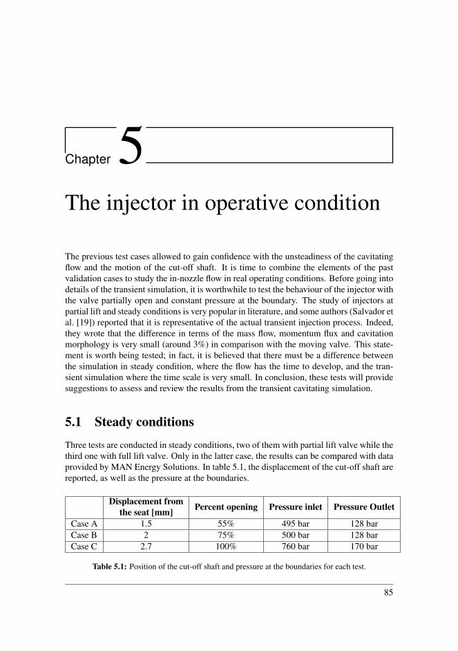
Chapter 5The injector in operative condition

The previous test cases allowed to gain confidence with the unsteadiness of the cavitatingflow and the motion of the cut-off shaft. It is time to combine the elements of the pastvalidation cases to study the in-nozzle flow in real operating conditions. Before going intodetails of the transient simulation, it is worthwhile to test the behaviour of the injector withthe valve partially open and constant pressure at the boundary. The study of injectors atpartial lift and steady conditions is very popular in literature, and some authors (Salvador etal. [19]) reported that it is representative of the actual transient injection process. Indeed,they wrote that the difference in terms of the mass flow, momentum flux and cavitationmorphology is very small (around 3%) in comparison with the moving valve. This state-ment is worth being tested; in fact, it is believed that there must be a difference betweenthe simulation in steady condition, where the flow has the time to develop, and the tran-sient simulation where the time scale is very small. In conclusion, these tests will providesuggestions to assess and review the results from the transient cavitating simulation.

5.1 Steady conditions

Three tests are conducted in steady conditions, two of them with partial lift valve while thethird one with full lift valve. Only in the latter case, the results can be compared with dataprovided by MAN Energy Solutions. In table 5.1, the displacement of the cut-off shaft arereported, as well as the pressure at the boundaries.

Displacement fromthe seat [mm] Percent opening Pressure inlet Pressure Outlet

Case A 1.5 55% 495 bar 128 barCase B 2 75% 500 bar 128 barCase C 2.7 100% 760 bar 170 bar

Table 5.1: Position of the cut-off shaft and pressure at the boundaries for each test.

85

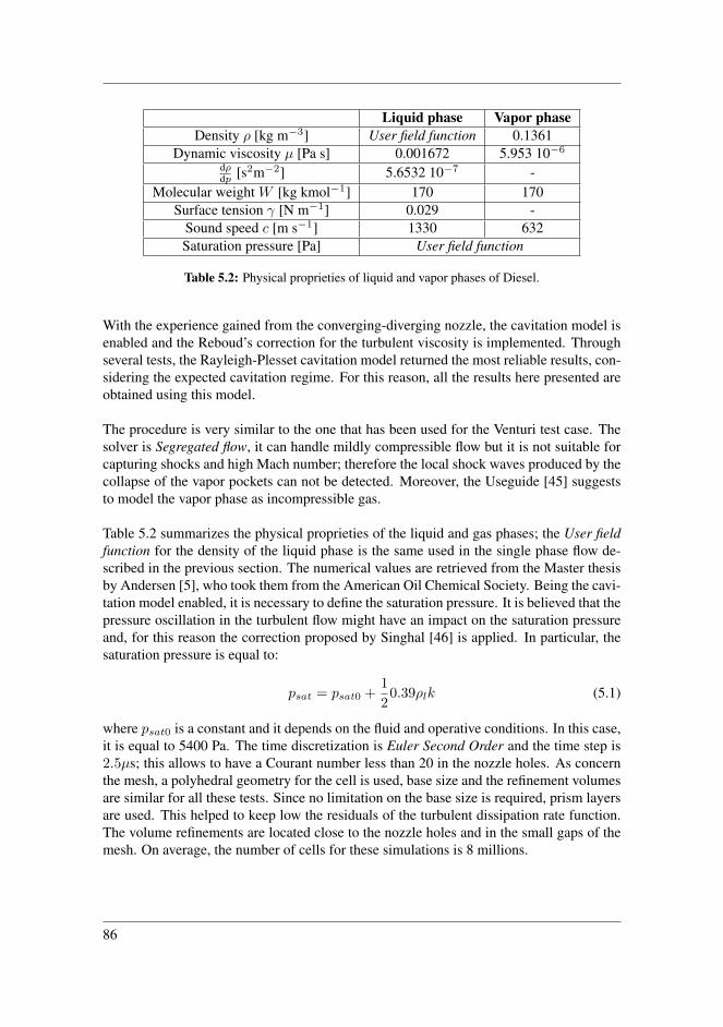
Liquid phase Vapor phaseDensity ρ [kg m−3] User field function 0.1361

Dynamic viscosity µ [Pa s] 0.001672 5.953 10−6

dρdp [s2m−2] 5.6532 10−7 -

Molecular weight W [kg kmol−1] 170 170Surface tension γ [N m−1] 0.029 -

Sound speed c [m s−1] 1330 632Saturation pressure [Pa] User field function

Table 5.2: Physical proprieties of liquid and vapor phases of Diesel.

With the experience gained from the converging-diverging nozzle, the cavitation model isenabled and the Reboud’s correction for the turbulent viscosity is implemented. Throughseveral tests, the Rayleigh-Plesset cavitation model returned the most reliable results, con-sidering the expected cavitation regime. For this reason, all the results here presented areobtained using this model.

The procedure is very similar to the one that has been used for the Venturi test case. Thesolver is Segregated flow, it can handle mildly compressible flow but it is not suitable forcapturing shocks and high Mach number; therefore the local shock waves produced by thecollapse of the vapor pockets can not be detected. Moreover, the Useguide [45] suggeststo model the vapor phase as incompressible gas.

Table 5.2 summarizes the physical proprieties of the liquid and gas phases; the User fieldfunction for the density of the liquid phase is the same used in the single phase flow de-scribed in the previous section. The numerical values are retrieved from the Master thesisby Andersen [5], who took them from the American Oil Chemical Society. Being the cavi-tation model enabled, it is necessary to define the saturation pressure. It is believed that thepressure oscillation in the turbulent flow might have an impact on the saturation pressureand, for this reason the correction proposed by Singhal [46] is applied. In particular, thesaturation pressure is equal to:

psat = psat0 +1

20.39ρlk (5.1)

where psat0 is a constant and it depends on the fluid and operative conditions. In this case,it is equal to 5400 Pa. The time discretization is Euler Second Order and the time step is2.5µs; this allows to have a Courant number less than 20 in the nozzle holes. As concernthe mesh, a polyhedral geometry for the cell is used, base size and the refinement volumesare similar for all these tests. Since no limitation on the base size is required, prism layersare used. This helped to keep low the residuals of the turbulent dissipation rate function.The volume refinements are located close to the nozzle holes and in the small gaps of themesh. On average, the number of cells for these simulations is 8 millions.

86

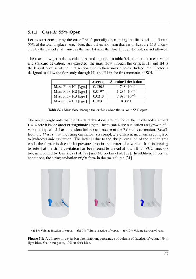
5.1.1 Case A: 55% OpenLet us start considering the cut-off shaft partially open, being the lift equal to 1.5 mm,55% of the total displacement. Note, that it does not mean that the orifices are 55% uncov-ered by the cut-off shaft, since in the first 1.4 mm, the flow through the holes is not allowed.

The mass flow per holes is calculated and reported in table 5.3, in terms of mean valueand standard deviation. As expected, the mass flow through the orifices H1 and H4 isthe largest because of the inlet section area in these nozzle holes. Indeed, the injector isdesigned to allow the flow only through H1 and H4 in the first moments of SOI.

Average Standard deviationMass Flow H1 [kg/s] 0.1305 4.748 ·10−4

Mass Flow H2 [kg/s] 0.0197 1.234 ·10−4

Mass Flow H3 [kg/s] 0.0213 7.985 ·10−5

Mass Flow H4 [kg/s] 0.1031 0.0041

Table 5.3: Mass flow through the orifices when the valve is 55% open.

The reader might note that the standard deviations are low for all the nozzle holes, exceptH4, where it is one order of magnitude larger. The reason is the nucleation and growth of avapor string, which has a transient behaviour because of the Reboud’s correction. Recall,from the Theory, that the string cavitation is a completely different mechanism comparedto hydrodynamic cavitation. The latter is due to the abrupt variation of the section areawhile the former is due to the pressure drop in the center of a vortex. It is interestingto note that the string cavitation has been found to prevail at low lift for VCO injectorstoo, as reported by Gavaises et al. [22] and Neroorkar et al. [37]. In addition, in certainconditions, the string cavitation might form in the sac volume [21].

(a) 1% Volume fraction of vapor. (b) 5% Volume fraction of vapor. (c) 10% Volume fraction of vapor.

Figure 5.1: A glimpse on cavitation phenomenon; percentage of volume of fraction of vapor; 1% inlight blue, 5% in magenta, 10% in dark blue.

87

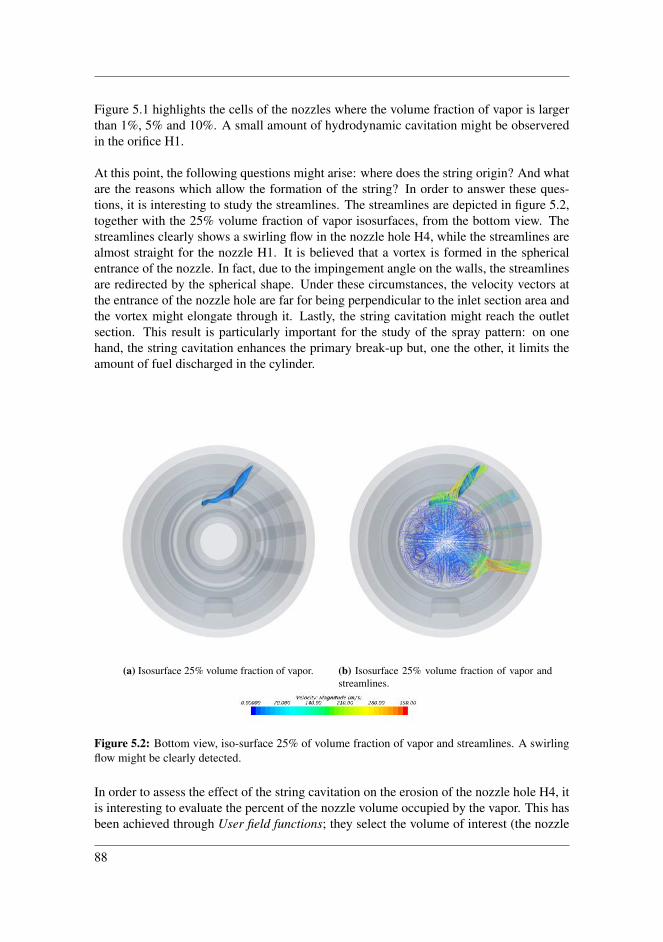
Figure 5.1 highlights the cells of the nozzles where the volume fraction of vapor is largerthan 1%, 5% and 10%. A small amount of hydrodynamic cavitation might be observeredin the orifice H1.

At this point, the following questions might arise: where does the string origin? And whatare the reasons which allow the formation of the string? In order to answer these ques-tions, it is interesting to study the streamlines. The streamlines are depicted in figure 5.2,together with the 25% volume fraction of vapor isosurfaces, from the bottom view. Thestreamlines clearly shows a swirling flow in the nozzle hole H4, while the streamlines arealmost straight for the nozzle H1. It is believed that a vortex is formed in the sphericalentrance of the nozzle. In fact, due to the impingement angle on the walls, the streamlinesare redirected by the spherical shape. Under these circumstances, the velocity vectors atthe entrance of the nozzle hole are far for being perpendicular to the inlet section area andthe vortex might elongate through it. Lastly, the string cavitation might reach the outletsection. This result is particularly important for the study of the spray pattern: on onehand, the string cavitation enhances the primary break-up but, one the other, it limits theamount of fuel discharged in the cylinder.

(a) Isosurface 25% volume fraction of vapor. (b) Isosurface 25% volume fraction of vapor andstreamlines.

Figure 5.2: Bottom view, iso-surface 25% of volume fraction of vapor and streamlines. A swirlingflow might be clearly detected.

In order to assess the effect of the string cavitation on the erosion of the nozzle hole H4, itis interesting to evaluate the percent of the nozzle volume occupied by the vapor. This hasbeen achieved through User field functions; they select the volume of interest (the nozzle

88

holes) and the amount of vapour is calculated integrating the volume fraction of vapor.Another parameter which deserves special attention is the vapor mass flow through thenozzle holes. It might return useful information for the investigation of the spray pattern.The results are summarized in table 5.4, where the mean value and standard deviation arereported. In figure 5.3, the volume fraction of vapor in four cylindrical sections of thenozzle H4 are plotted.

NozzleHole

Percentage Volume Vapor Mass flowAverage [%] Std. deviation [%] Average [mg/s] Std. deviation [mg/s]

H1 0.425 0.038 0.0912 0.0116H2 0.012 0.004 - -H3 0.019 0.01 - -H4 11.65 0.47 2.190 0.170

Table 5.4: Percentage of volume occupied by the vapor in the nozzle holes and phase mass flowthrough the four orifices.

Figure 5.3: Volume fraction of vapour in four cylindrical section of the nozzle hole. The referenceradii of the cylindrical surfaces coaxial with the injector are 3.5 mm, 4.5 mm, 5.5 mm, 6.5 mm.

Lastly, in figure 5.4 and 5.5 the velocity and the pressure field are depicted in planesintersecting the nozzles’ axes and parallel to the injector’s axis.

89

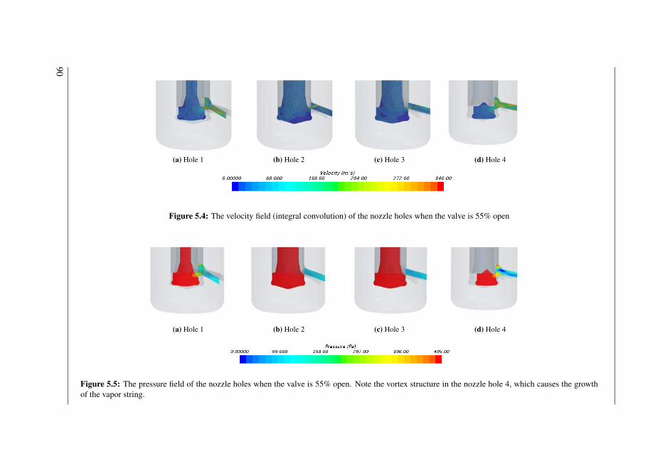
(a) Hole 1 (b) Hole 2 (c) Hole 3 (d) Hole 4

Figure 5.4: The velocity field (integral convolution) of the nozzle holes when the valve is 55% open

(a) Hole 1 (b) Hole 2 (c) Hole 3 (d) Hole 4

Figure 5.5: The pressure field of the nozzle holes when the valve is 55% open. Note the vortex structure in the nozzle hole 4, which causes the growthof the vapor string.

90

5.1.2 Case B: 75% OpenThe displacement of the cut-off shaft from the seat is now equal to 2 mm, 75% of the totallift. As expected, the mass flow through the orifices is larger than the previous case; themean values and the standard deviations are calculated and summarized in table 5.5.

Average Standard deviationMass Flow H1 [kg/s] 0.1650 1.518 · 10−4

Mass Flow H2 [kg/s] 0.1229 0.0023Mass Flow H3 [kg/s] 0.1213 2.747 · 10−4

Mass Flow H4 [kg/s] 0.1683 7.046 · 10−4

Table 5.5: Mass flow through the orifices when the valve is 75% open.

As it might be observed from figure 5.6, all the nozzle holes exhibit a change of phase, dueto cavitation. In particular, the orifices H2, H3 and H4 experience the toughest cavitationregime. From the analysis of the scalar field volume fraction if vapor, the hydrodynamiccavitation is observed in H2 and H3. In the latter, a string forms behind the portion ofthe cut-off shaft which still covers the orifice. The string combines with the cavity pocketdue to hydrodynamic cavitation and elongates until the outlet section. String cavitationand swirling flow is still present in nozzle H4. The swirling flow seems to have a largeintensity in nozzle H3 too. Table 5.5 shows that the standard deviation is quite low for allthe nozzles except H2; here the standard deviation is one order of magnitude larger thanthe others. The analysis of the mass flow for this nozzle hole show a periodic sheddingwith a frequency equal to 7600 Hz.

(a) 1% Volume fraction of vapor. (b) 5% Volume fraction of vapor. (c) 10% Volume fraction of vapor.

Figure 5.6: A glimpse on the cavitation phenomenon, percentage of volume of fraction of vapor;1% in light blue, 5% in magenta, 10% in dark blue.

The streamlines and the isosurfaces for the volume fraction 5% are depicted in figure 5.7,

91

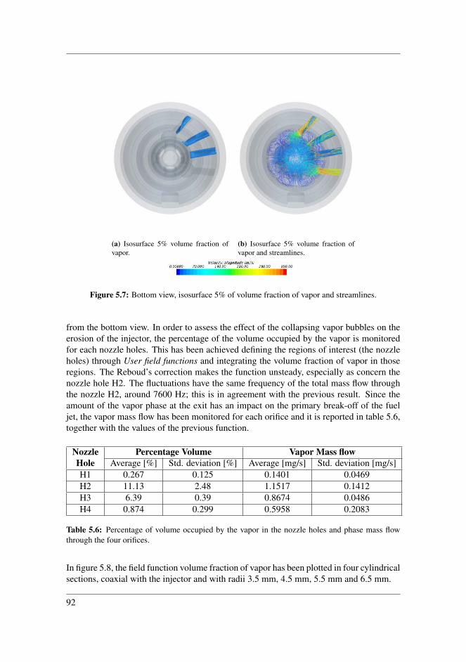
(a) Isosurface 5% volume fraction ofvapor.

(b) Isosurface 5% volume fraction ofvapor and streamlines.

Figure 5.7: Bottom view, isosurface 5% of volume fraction of vapor and streamlines.

from the bottom view. In order to assess the effect of the collapsing vapor bubbles on theerosion of the injector, the percentage of the volume occupied by the vapor is monitoredfor each nozzle holes. This has been achieved defining the regions of interest (the nozzleholes) through User field functions and integrating the volume fraction of vapor in thoseregions. The Reboud’s correction makes the function unsteady, especially as concern thenozzle hole H2. The fluctuations have the same frequency of the total mass flow throughthe nozzle H2, around 7600 Hz; this is in agreement with the previous result. Since theamount of the vapor phase at the exit has an impact on the primary break-off of the fueljet, the vapor mass flow has been monitored for each orifice and it is reported in table 5.6,together with the values of the previous function.

NozzleHole

Percentage Volume Vapor Mass flowAverage [%] Std. deviation [%] Average [mg/s] Std. deviation [mg/s]

H1 0.267 0.125 0.1401 0.0469H2 11.13 2.48 1.1517 0.1412H3 6.39 0.39 0.8674 0.0486H4 0.874 0.299 0.5958 0.2083

Table 5.6: Percentage of volume occupied by the vapor in the nozzle holes and phase mass flowthrough the four orifices.

In figure 5.8, the field function volume fraction of vapor has been plotted in four cylindricalsections, coaxial with the injector and with radii 3.5 mm, 4.5 mm, 5.5 mm and 6.5 mm.

92

(a) Hole 1

(b) Hole 2

(c) Hole 3

(d) Hole 4

Figure 5.8: Iso-surface (10% of the volume fraction of vapor) and streamlines when the valve is75% open

The velocity and the pressure field in quasi-steady state is reported in figure 5.9 and 5.10for each orifices, in the section plane intersecting the nozzle’s axis.

93

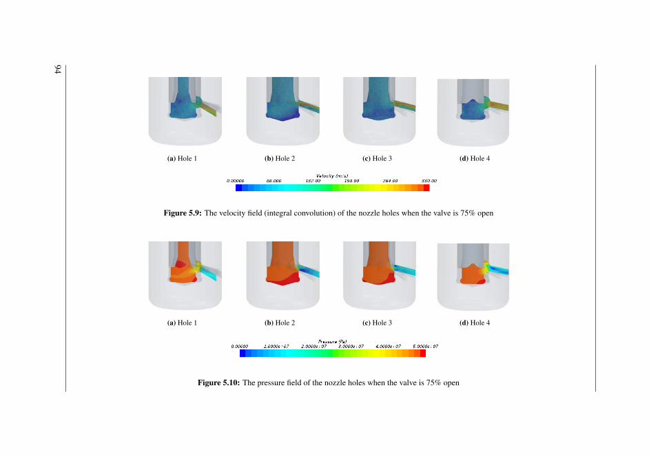
(a) Hole 1 (b) Hole 2 (c) Hole 3 (d) Hole 4

Figure 5.9: The velocity field (integral convolution) of the nozzle holes when the valve is 75% open

(a) Hole 1 (b) Hole 2 (c) Hole 3 (d) Hole 4

Figure 5.10: The pressure field of the nozzle holes when the valve is 75% open

94

5.1.3 Case C: 100% Open

Among the simulations in steady conditions, the case with the valve completely open isthe most relevant. In fact, it is the only test aimed at reproducing the actual operativecondition of the injector. When the fuel valve is fully open in the injection process, thesteady condition is achieved. In addition to that, this test allows to make an assessment ofthe model against the data from MAN Energy Solutions. The company provided a chartwhich relates the discharge coefficient with the square root of the cavitation number K.Firstly, it is convenient to calculate the cavitation number in order to predict the cavitationregime. The cavitation number CN is equal to:

CN =pi − popo − psat

=(722− 170) · 105

170 · 105 − 5400= 3.25 (5.2)

where the inlet pressure, pi, is recorded by a probe located in the sac volume. From thechart in figure 2.5, which relates the inverse of the cavitation number, CN−1 with the cav-itation length, the super-cavitation regime is expected. A vapor film should form aroundthe wall of the nozzles holes and it should reach the outlet section. It is likely to happen innozzles H2 and H3, where there is an abrupt variation in the section area from the sac to theentrance of the orifices. The smooth curvature around the inlet of H1 and H4 should makecavitation unlikely to appear; in addition to that, the nozzle H1 and H4 are slightly longerthan the other two and it contributes to increase the pressure in the region of vena contracta.

Once that the steady condition has been reached, the average and the standard deviation ofthe mass flow can be evaluated. The mean value and the standard deviation are calculatedand presented in table 5.7:

Average Standard deviationMass Flow H1 [kg/s] 0.2061 0.003Mass Flow H2 [kg/s] 0.1989 0.006Mass Flow H3 [kg/s] 0.2054 0.002Mass Flow H4 [kg/s] 0.2240 0.002

Table 5.7: Mass flow through the orifices when the valve is at full lift.

In order to make an assessment against the data from MAN, the discharge coefficient, Cd,must be calculated. Recall the definition of this non dimensional quantity: it is the ratiobetween the actual and the theoretical mass flow:

Cd =m

AoρUb(5.3)

where Ub is the velocity in the outlet section and it is calculated from the Bernoulli equa-tion (see eq.(2.1)):

Ub =

√2(pi − po)

ρ(5.4)

95

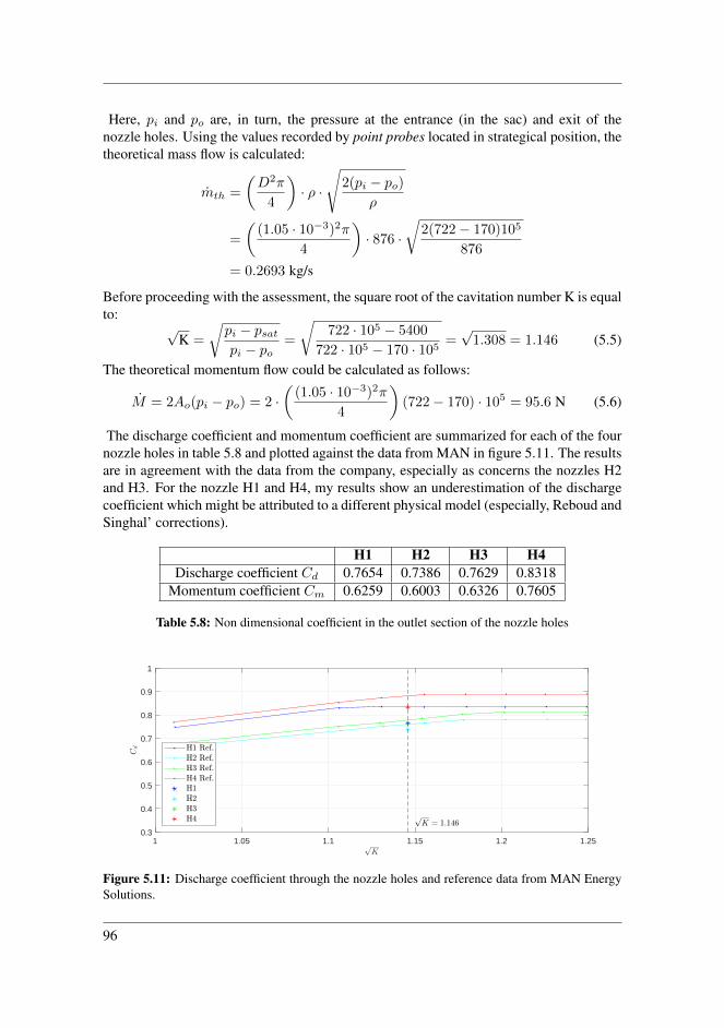
Here, pi and po are, in turn, the pressure at the entrance (in the sac) and exit of thenozzle holes. Using the values recorded by point probes located in strategical position, thetheoretical mass flow is calculated:

mth =

(D2π

4

)· ρ ·

√2(pi − po)

ρ

=

((1.05 · 10−3)2π

4

)· 876 ·

√2(722− 170)105

876

= 0.2693 kg/s

Before proceeding with the assessment, the square root of the cavitation number K is equalto:

√K =

√pi − psatpi − po

=

√722 · 105 − 5400

722 · 105 − 170 · 105=√

1.308 = 1.146 (5.5)

The theoretical momentum flow could be calculated as follows:

M = 2Ao(pi − po) = 2 ·(

(1.05 · 10−3)2π

4

)(722− 170) · 105 = 95.6 N (5.6)

The discharge coefficient and momentum coefficient are summarized for each of the fournozzle holes in table 5.8 and plotted against the data from MAN in figure 5.11. The resultsare in agreement with the data from the company, especially as concerns the nozzles H2and H3. For the nozzle H1 and H4, my results show an underestimation of the dischargecoefficient which might be attributed to a different physical model (especially, Reboud andSinghal’ corrections).

H1 H2 H3 H4Discharge coefficient Cd 0.7654 0.7386 0.7629 0.8318

Momentum coefficient Cm 0.6259 0.6003 0.6326 0.7605

Table 5.8: Non dimensional coefficient in the outlet section of the nozzle holes

1 1.05 1.1 1.15 1.2 1.25

0.3

0.4

0.5

0.6

0.7

0.8

0.9

1

Figure 5.11: Discharge coefficient through the nozzle holes and reference data from MAN EnergySolutions.

96

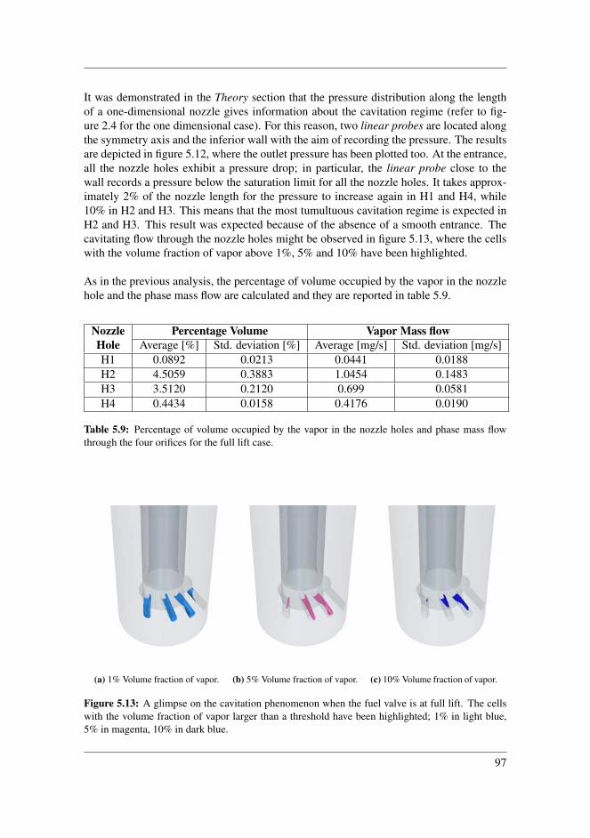
It was demonstrated in the Theory section that the pressure distribution along the lengthof a one-dimensional nozzle gives information about the cavitation regime (refer to fig-ure 2.4 for the one dimensional case). For this reason, two linear probes are located alongthe symmetry axis and the inferior wall with the aim of recording the pressure. The resultsare depicted in figure 5.12, where the outlet pressure has been plotted too. At the entrance,all the nozzle holes exhibit a pressure drop; in particular, the linear probe close to thewall records a pressure below the saturation limit for all the nozzle holes. It takes approx-imately 2% of the nozzle length for the pressure to increase again in H1 and H4, while10% in H2 and H3. This means that the most tumultuous cavitation regime is expected inH2 and H3. This result was expected because of the absence of a smooth entrance. Thecavitating flow through the nozzle holes might be observed in figure 5.13, where the cellswith the volume fraction of vapor above 1%, 5% and 10% have been highlighted.

As in the previous analysis, the percentage of volume occupied by the vapor in the nozzlehole and the phase mass flow are calculated and they are reported in table 5.9.

NozzleHole

Percentage Volume Vapor Mass flowAverage [%] Std. deviation [%] Average [mg/s] Std. deviation [mg/s]

H1 0.0892 0.0213 0.0441 0.0188H2 4.5059 0.3883 1.0454 0.1483H3 3.5120 0.2120 0.699 0.0581H4 0.4434 0.0158 0.4176 0.0190

Table 5.9: Percentage of volume occupied by the vapor in the nozzle holes and phase mass flowthrough the four orifices for the full lift case.

(a) 1% Volume fraction of vapor. (b) 5% Volume fraction of vapor. (c) 10% Volume fraction of vapor.

Figure 5.13: A glimpse on the cavitation phenomenon when the fuel valve is at full lift. The cellswith the volume fraction of vapor larger than a threshold have been highlighted; 1% in light blue,5% in magenta, 10% in dark blue.

97

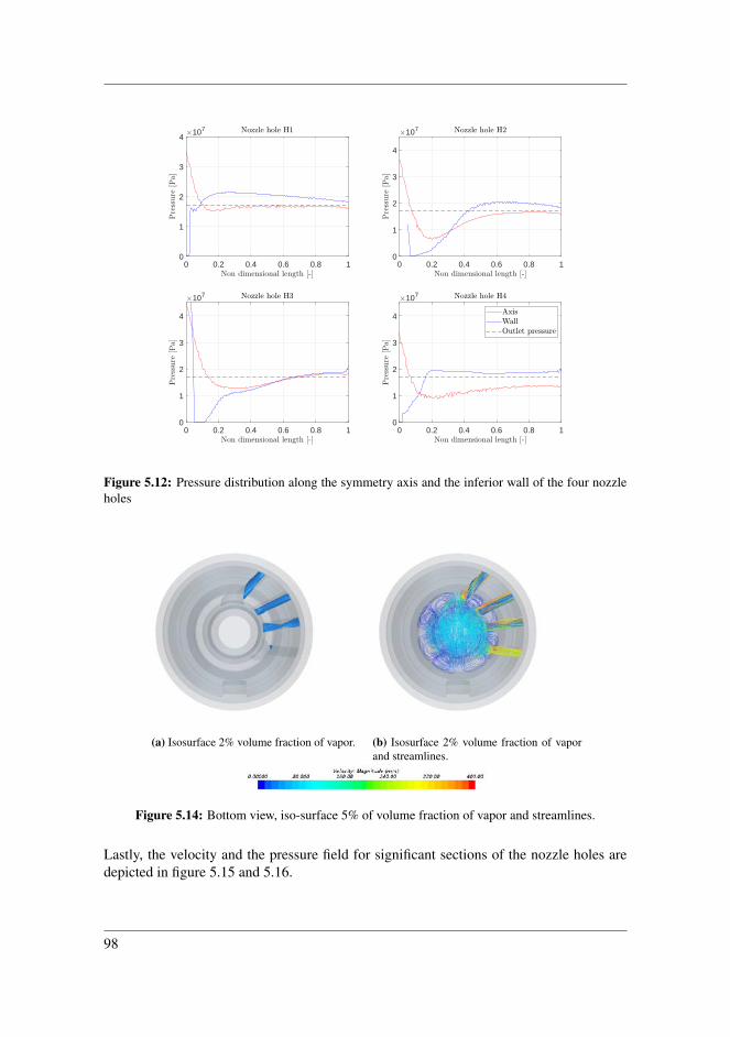
0 0.2 0.4 0.6 0.8 1

0

1

2

3

410

7

0 0.2 0.4 0.6 0.8 1

0

1

2

3

4

107

0 0.2 0.4 0.6 0.8 1

0

1

2

3

4

107

0 0.2 0.4 0.6 0.8 1

0

1

2

3

4

107

Figure 5.12: Pressure distribution along the symmetry axis and the inferior wall of the four nozzleholes

(a) Isosurface 2% volume fraction of vapor. (b) Isosurface 2% volume fraction of vaporand streamlines.

Figure 5.14: Bottom view, iso-surface 5% of volume fraction of vapor and streamlines.

Lastly, the velocity and the pressure field for significant sections of the nozzle holes aredepicted in figure 5.15 and 5.16.

98

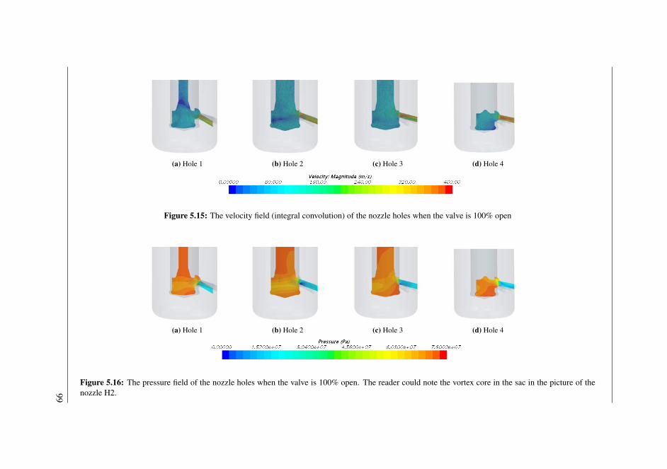
(a) Hole 1 (b) Hole 2 (c) Hole 3 (d) Hole 4

Figure 5.15: The velocity field (integral convolution) of the nozzle holes when the valve is 100% open

(a) Hole 1 (b) Hole 2 (c) Hole 3 (d) Hole 4

Figure 5.16: The pressure field of the nozzle holes when the valve is 100% open. The reader could note the vortex core in the sac in the picture of thenozzle H2.99

5.2 Transient simulationThe previous simulations were run in steady conditions, meaning that the needle was stilland the pressure at the boundaries was constant. The next step consists in introducing theactual operative pressure conditions and the motion of the cut-off shaft by means of theoverset technology. Because of the EOI limitations discussed in the previous chapter, onlythe SOI will be considered.

The trimmer mesh is used in this analysis since it is optimized to operate with the over-set technology being the ”scaling” geometries only close to the edges of the orifices. Thephysical proprieties of the liquid and vapor phases are equal to those presented in table 4.5,while the reader might refer to figure 4.28 and 4.29 for the lift and the pressures at theboundaries versus time. The full Rayleigh-Plesset cavitation model is used. The transientanalysis is aimed at answering the following questions: does the seat exhibit cavitation inthe first moments of the opening as reported by several authors [8]? What is the relation-ship between the volume fraction of vapor and the lift? Lastly, is true that the differencebetween the transient and steady simulation might be negligible? Before start answeringthese questions, let us have a look at the mass flow and the momentum flow in figure 5.17and 5.18 respectively.

0 0.5 1 1.5 2 2.5 3

0

0.2

0.4

0.6

0.8

1

0

0.5

1

1.5

2

Figure 5.17: Mass flow through the four orifices and total mass flow versus time.

The plots of the mass and momentum flow look similar to those presented in the singlephase flow during the opening of the fuel valve. In addition to that, even if the steadyconditions have not been achieved yet, the mass and momentum flow in the last time stepare in agreement with the values from the steady simulation and full lift. The fluctuationsare due to the pressure wave travelling back and forth in the system with a frequency ofaround 3300 Hz, in a similar way of what has been discussed in the single phase flowvalidation case.

The solution is recorded in a .simh history file and the first instant of the disclosure eventis reported in figure 5.19 for the velocity field, zooming on the seat. Being the geometryaxisymmetric above the seat, only a section of the entire fluid domain is considered. Dueto the pressure difference between the room above and below the seat, the velocity reaches

100

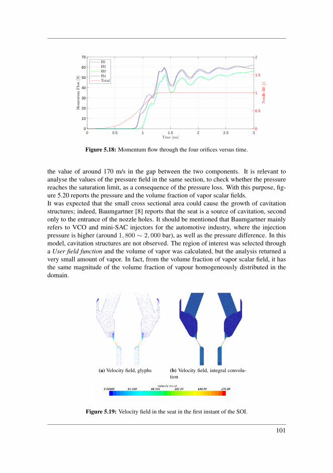
0 0.5 1 1.5 2 2.5 3

0

10

20

30

40

50

60

70

0

0.5

1

1.5

2

Figure 5.18: Momentum flow through the four orifices versus time.

the value of around 170 m/s in the gap between the two components. It is relevant toanalyse the values of the pressure field in the same section, to check whether the pressurereaches the saturation limit, as a consequence of the pressure loss. With this purpose, fig-ure 5.20 reports the pressure and the volume fraction of vapor scalar fields.It was expected that the small cross sectional area could cause the growth of cavitationstructures; indeed, Baumgartner [8] reports that the seat is a source of cavitation, secondonly to the entrance of the nozzle holes. It should be mentioned that Baumgartner mainlyrefers to VCO and mini-SAC injectors for the automotive industry, where the injectionpressure is higher (around 1, 800 ∼ 2, 000 bar), as well as the pressure difference. In thismodel, cavitation structures are not observed. The region of interest was selected througha User field function and the volume of vapor was calculated, but the analysis returned avery small amount of vapor. In fact, from the volume fraction of vapor scalar field, it hasthe same magnitude of the volume fraction of vapour homogeneously distributed in thedomain.

(a) Velocity field, glyphs (b) Velocity field, integral convolu-tion

Figure 5.19: Velocity field in the seat in the first instant of the SOI.

101

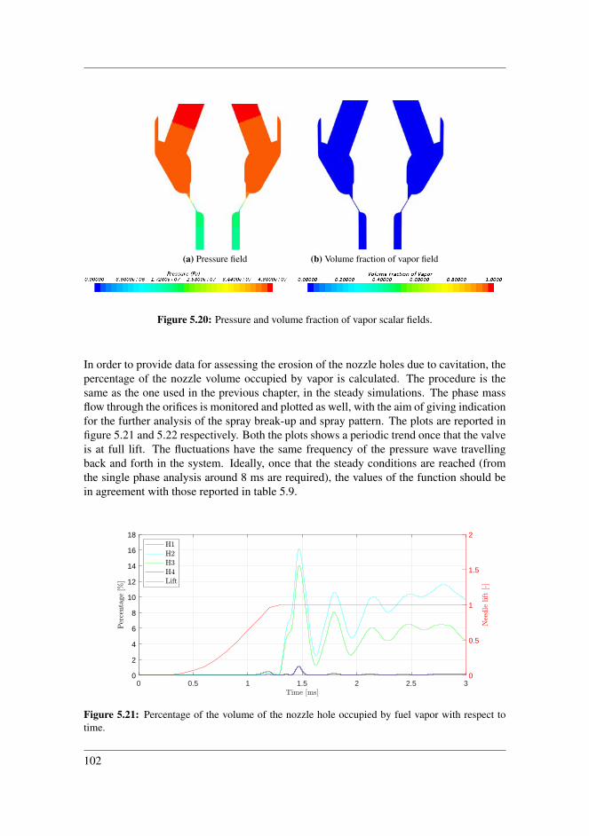
(a) Pressure field (b) Volume fraction of vapor field

Figure 5.20: Pressure and volume fraction of vapor scalar fields.

In order to provide data for assessing the erosion of the nozzle holes due to cavitation, thepercentage of the nozzle volume occupied by vapor is calculated. The procedure is thesame as the one used in the previous chapter, in the steady simulations. The phase massflow through the orifices is monitored and plotted as well, with the aim of giving indicationfor the further analysis of the spray break-up and spray pattern. The plots are reported infigure 5.21 and 5.22 respectively. Both the plots shows a periodic trend once that the valveis at full lift. The fluctuations have the same frequency of the pressure wave travellingback and forth in the system. Ideally, once that the steady conditions are reached (fromthe single phase analysis around 8 ms are required), the values of the function should bein agreement with those reported in table 5.9.

0 0.5 1 1.5 2 2.5 3

0

2

4

6

8

10

12

14

16

18

0

0.5

1

1.5

2

Figure 5.21: Percentage of the volume of the nozzle hole occupied by fuel vapor with respect totime.

102

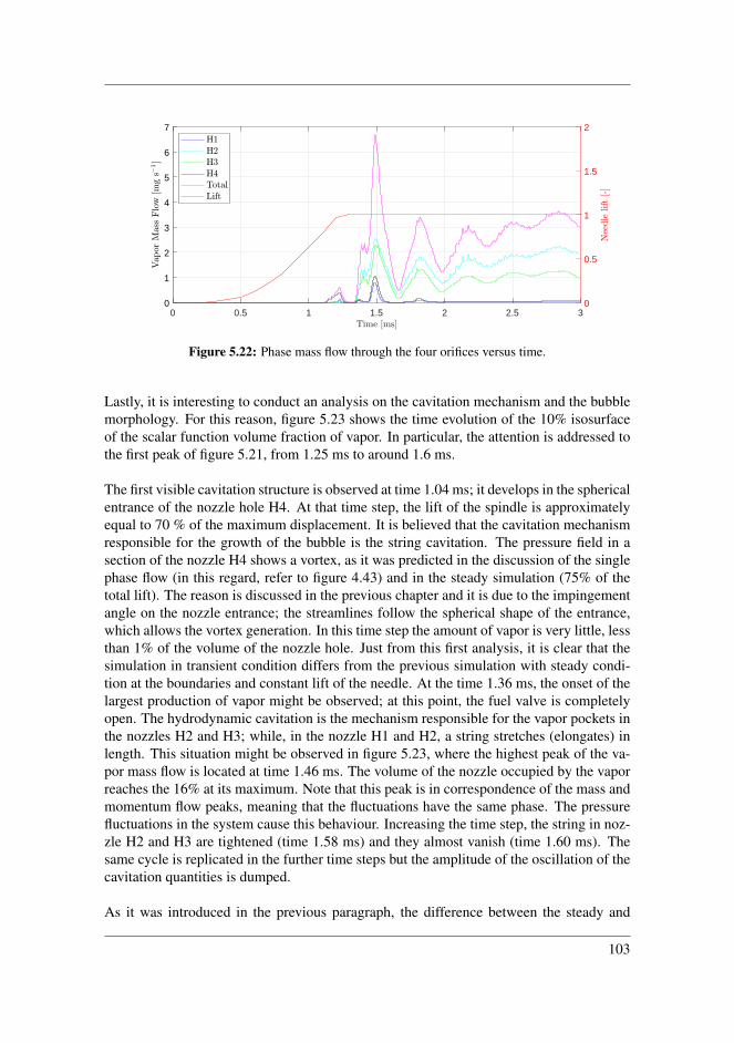
0 0.5 1 1.5 2 2.5 3

0

1

2

3

4

5

6

7

0

0.5

1

1.5

2

Figure 5.22: Phase mass flow through the four orifices versus time.

Lastly, it is interesting to conduct an analysis on the cavitation mechanism and the bubblemorphology. For this reason, figure 5.23 shows the time evolution of the 10% isosurfaceof the scalar function volume fraction of vapor. In particular, the attention is addressed tothe first peak of figure 5.21, from 1.25 ms to around 1.6 ms.

The first visible cavitation structure is observed at time 1.04 ms; it develops in the sphericalentrance of the nozzle hole H4. At that time step, the lift of the spindle is approximatelyequal to 70 % of the maximum displacement. It is believed that the cavitation mechanismresponsible for the growth of the bubble is the string cavitation. The pressure field in asection of the nozzle H4 shows a vortex, as it was predicted in the discussion of the singlephase flow (in this regard, refer to figure 4.43) and in the steady simulation (75% of thetotal lift). The reason is discussed in the previous chapter and it is due to the impingementangle on the nozzle entrance; the streamlines follow the spherical shape of the entrance,which allows the vortex generation. In this time step the amount of vapor is very little, lessthan 1% of the volume of the nozzle hole. Just from this first analysis, it is clear that thesimulation in transient condition differs from the previous simulation with steady condi-tion at the boundaries and constant lift of the needle. At the time 1.36 ms, the onset of thelargest production of vapor might be observed; at this point, the fuel valve is completelyopen. The hydrodynamic cavitation is the mechanism responsible for the vapor pockets inthe nozzles H2 and H3; while, in the nozzle H1 and H2, a string stretches (elongates) inlength. This situation might be observed in figure 5.23, where the highest peak of the va-por mass flow is located at time 1.46 ms. The volume of the nozzle occupied by the vaporreaches the 16% at its maximum. Note that this peak is in correspondence of the mass andmomentum flow peaks, meaning that the fluctuations have the same phase. The pressurefluctuations in the system cause this behaviour. Increasing the time step, the string in noz-zle H2 and H3 are tightened (time 1.58 ms) and they almost vanish (time 1.60 ms). Thesame cycle is replicated in the further time steps but the amplitude of the oscillation of thecavitation quantities is dumped.

As it was introduced in the previous paragraph, the difference between the steady and

103

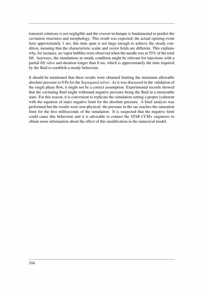
transient solutions is not negligible and the overset technique is fundamental to predict thecavitation structures and morphology. This result was expected; the actual opening eventlasts approximately 1 ms; this time span is not large enough to achieve the steady con-dition, meaning that the characteristic scalar and vector fields are different. This explainswhy, for instance, no vapor bubbles were observed when the needle was at 55% of the totallift. Anyways, the simulations in steady condition might be relevant for injections with apartial lift valve and duration longer than 8 ms, which is approximately the time requiredby the fluid to establish a steady behaviour.

It should be mentioned that these results were obtained limiting the minimum allowableabsolute pressure to 0 Pa for the Segregated solver. As it was discussed in the validation ofthe single phase flow, it might not be a correct assumption. Experimental records showedthat the cavitating fluid might withstand negative pressure being the fluid in a metastablestate. For this reason, it is convenient to replicate the simulation setting a proper (coherentwith the equation of state) negative limit for the absolute pressure. A brief analysis wasperformed but the results were non-physical: the pressure in the sac reaches the saturationlimit for the first milliseconds of the simulation. It is suspected that the negative limitcould cause this behaviour and it is advisable to contact the STAR CCM+ engineers toobtain more information about the effect of this modification in the numerical model.

104

(a) t = 1.04 ms (b) t = 1.30 ms (c) t = 1.36 ms (d) t = 1.42 ms

(e) t = 1.46 ms (f) t = 1.48 ms (g) t = 1.58 ms (h) t = 1.60 ms

Figure 5.23: 10% volume fraction of vapor isosurface. Visualization of the cavitation regime in the first peak of figure 5.21.

105

106

Chapter 6Conclusion

The study of this Master thesis allows to develop and tune-up a numerical CFD model forthe in-nozzle flow during the opening and closing of the fuel valve. The overset techniqueis the technology chosen to reproduce the motion of the valve. The choice of the overset isjustified by the good resolution of the small gaps during the entire transient process; thisfeature might not be fulfilled with other techniques. In addition to that, the Userguide ofSTAR CCM+ [45] suggests to use this technique in case of opening and closing of valves.

Experiments about the actual injection conditions are not possible due to the high pres-sures involved in the process, the need of use optical technique to detect and study themorphology of the vapor bubbles, the dimensions of the nozzle holes and the fluid veloc-ity (around 0.3∼0.4 Ma). Therefore, only little information is available in literature. Thislack of information forces to take a step back and validate the numerical model.

The first validation is about the transient cavitation; in fact, high transient cavitation struc-tures are expected at the opening of the fuel valve. The question which arises is whetherthe standard cavitation model could reproduce correctly the dynamics of the vapor bubbles.For this reason, after a wide research in the literature, the experimental periodic cavitat-ing flow inside a converging-diverging Venturi nozzle [28] is simulated numerically. Themain assumptions of this test case are the use of the Unsteady Reynolds Averaged Navier-Stokes equations (URANS), the Eulerian multiphase Volume of Fraction method (VOF)and the axysimmetry. It is discovered that the turbulence model plays a relevant role inthe shedding process. The large values of the turbulent viscosity do not permit to get thedetachment of the vapor pocket; for this reason the correction proposed by Reboud is in-troduced. It consists in multiplying the turbulent viscosity by a scaling factor, which isfunction of the density field. This allows to reproduce the physics of the phenomenon witha larger accuracy and, in the best solution, the relative error of the shedding frequency islimited to 6%.

The second validation case is about the single phase flow in the injector during the tran-

107

sients, at the opening and closing of the fuel valve. The results are compared with a in-house code by MAN Energy Solutions named 1D-Hydcode. The lack of the experimentaldata forces to use some of the output of the one-dimensional code as input in the CFD sim-ulation. The opening event is well represented; through the use of the Overset Zero GapInterface technology, the first instant of the opening is correctly detected. The mass flowand the pressure in the sac volume show a satisfying agreement with the 1D-Hydecode.The plots of these quantities exhibit a phase displacement due to the different frequenciesof the pressure wave travelling through the system. This result was expected consideringthat in the CFD simulation only three component of the full system are considered, whilethe 1D-Hydcode is aimed at modelling the entire injector. In this analysis a vortex is ob-served in the sac volume; its core changes orientation with respect to time. In particular,when the steady conditions are achieved, it is aligned with two nozzle holes of the injec-tor, leading to large fluctuations in mass and momentum flow. The results from the end ofinjection event can not be trusted; in this case, the misalignment between the hypothesesof the one-dimensional code and the CFD simulation (absence of EDM, different lengthof the system and, above all, the fact that in one model the motion is the consequence ofthe pressure acting on the surfaces of the cut-off shaft while in the other it is prescribed)leads to reversed flow and negative mass flow.

Before moving on to the transient and multiphase simulation, three tests were conductedwith the valve partially open and at full lift. These test are aimed at checking whether thereis a large difference in the cavitation morphology and in the mass and momentum valuescompared to the transient simulation. They permit to discover that different cavitationmechanisms appear in the nozzle holes. When the valve is a low lift, the string cavitationmechanism dominates; especially as regard the two nozzle holes having a spherical en-trance. The impingement angle on the wall causes a vortex which stretches and elongatesin the nozzles. A mix of vortex and hydrodynamic cavitation is observed when the spindleis at 75% of the total lift, while hydrodynamic cavitation prevails when the valve is at fulllift. For each of these cases, the mass and momentum flow is calculated, as well as the vol-ume occupied in the nozzle holes and the phase mass flow. These quantities will providerelevant information for further possible investigation of the erosion of the nozzles’ wallsdue to the collapse of the vapor bubbles and the break-up of the fuel jet.

Lastly, the simulation with the moving valve and cavitation model is run. The amountof vapor follows the trend given by the pressure fluctuations in the fluid domain. Con-trary to expectations, cavitation in the seat is not observed. The lack of experimental datadoes not allow to make safe statement, but it is believed that prescribing the motion ofthe spindle might have an effect on the cavitation in the gap between seat and spindle. Asit will be widely discussed in the next chapter, further investigation should be conductedimplementing the DFBI (Dynamic Fluid-Body Interaction) option, and coupling the cut-off shaft with a one-dimensional linear spring. In this way, the motion of the shaft mightbe due to the forces acting on it. The time evolution of the cavitation structure allows toconclude that the hydrodynamic cavitation prevails in the process but string cavitation ispresent in the nozzles with a smooth entrance too. The percentage of volume of the nozzlehole occupied by fuel vapor and the fuel vapor mass flow for each of the nozzle holes is

108

monitored and plotted versus time; providing information for further analyses.

6.1 Recommendations for the FutureWith the experience gained working in the project, these improvements of the CFD modelare suggested. Let us start from the mesh. The geometry of the moving part (the spindle)is quite complex; it is hollowed and it is not axisymmetric. The overset mesh was createdsimply reproducing the shape of the needle and using the Bolean operation subtract. Thismethod works fine but it returns quite a loose fit; as a consequence of that, the mesh ofoverset is heavy and it has an impact on the CPU time. For this reason, I suggest to use atighter fit. In this regard, some CAD software (for instance, Solidworks) allows to createoffset surface from the actual body’s surface. I believe that the tighter fit mesh might helpin achieving the convergence of rate of dissipation term too.

It is important to recall that the overset technique is not mass conservative; in general,the error is negligible but, for this application, it is advisable to turn on the method Fluxcorrection for compressible flow to enforce the continuity.

Further developments of the physical model might consist in coupling the one-dimensionalcode 1D-Hydcode and STAR CCM+; in this way, the dynamic effects in the entire systemmight be replicated numerically. In this regard, instead of prescribing the motion, it mightbe convenient to model the motion of the spindle as a consequence of the pressure actingon its surfaces. This might be achieved using the DFBI (Dynamic Fluid Body Interaction)options; in particular, allowing the translation in the vertical coordinate (system with onedegree of freedom) and modelling a linear spring coupling.

Once that the in-nozzle flow has been investigated, it is interesting to study the spray de-velopment in the cylinder too. Some numerical correlations between the needle position,cavitation structures and spray angle (or penetration length, Mean Sauer Diameter, . . . )might be derived.

On the experimental side, it would be convenient to test the geometry of this project inthe steady state rig and compare the results with the CFD solutions for the partial lift tests.In this way, the different cavitation mechanisms might be investigated experimentally too.

109

110

Bibliography

[1] https://www.youtube.com/watch?v=sHTf2wzDqVY, Accessed May 19,2019.

[2] https://www.youtube.com/watch?v=7Y1rCU3kUm0, Accessed May 19,2019.

[3] https://www.dieselnet.com/standards/inter/imo.php, AccessedMay 7, 2019.

[4] https://www.cfdsupport.com/OpenFOAM-Training-by-CFD-Support/node199.html, Accessed May 8, 2019.

[5] F. H. Andersen. Numerical simulation of flow in fuel nozzles for two stroke dieselengines, 2011.

[6] E. H. Atta and J. Vadyak. A grid overlapping scheme for flowfield computationsabout multicomponent configurations. American Institute of Aeronautics and Astro-nautics, 21(9):1271–1277, 1983.

[7] C. Badock, R. Wirth, A. Fath, and A. Leipertz. Investigation of cavitation in real sizediesel injector nozzle. International Journal of Heat and Fluid Flow, 20(5):538–544,1999.

[8] Baumgartner. Mixture Formation in Internal Combustion Engines. Springer, 2006.

[9] R. Benson. The Thermodynamics of gas dynamics of internal combustion engine.Clarendon Press Oxford, 1982.

[10] W. Bergwerk. Flow pattern in diesel nozzle spray holes. Proceedings of the Institu-tion of Mechanical Engineers, 173(25):655–660, 1959.

[11] H. B. Bingham, P. Larsen, and A. Barker. Lecture Notes for CFD Course. DTUMekanik, 2018.

111

[12] M. Blessing, G. Konig, C. Kruger, U. Micheals, and V. Schwarz. Analysis of flowand cavitation phenomena in diesel injection nozzles and its effects on spray andmixture formation. SAE International, 1(1358), 2003.

[13] D. Bonilla, J. D. K. Bishop, C. J. Axon, and D. Banister. Innovation, the diesel engineand vehicle markets: Evidence from oecd engine patents. Transportation Research,27:51–58, 2014.

[14] C. E. Brenner. Cavitation and Bubble Dynamics. Oxford University Press, 1995.

[15] M. Callenaere, J. Franc, J. Michel, and M. Riondet. The cavitation instability inducedby the development of a re-entrant jet. Journal of Fluid Mechanics, 444:223–256,2001.

[16] Y. Cengel, J. Cimbala, G. Cozzo, and C. Santoro. Meccanica dei Fluidi. McGrawHill Educational, 3 edition, 2015.

[17] O. Coutier-Delgosha, R. Fortes-Patella, and J. Reboud. Evaluation of the turbulencemodel influence on the numerical simulation of unsteady cavitation. ASME, 125,2003.

[18] B. Dam. Experimental and numerical investigations of sprays in two stroke dieselengines, 2007.

[19] J. M. Desantes, F. Salvador, M. Carreres, and J. Martinez-Lopez. Large eddy simu-lation analysis of the influence of the needle lift on the cavitation in diesel injectornozzles. Journal of Automobile Engineering, 229(4):407–423, 2014.

[20] J. Ferziger and M. Peric. Computational Methods for Fluid Dynamics. Springer,2002.

[21] M. Gavaises, A. Andriotis, and C. Arcoumanis. Vortex flow and cavitation in dieselinjector nozzles. Journal of Fluid Mechanics, 610:195–215, 2008.

[22] M. Gavaises, A. Andriotis, D. Papoulias, M. N., and A. Theodorakakos. Character-ization of string cavitation in large-scale diesel nozzles with taperad holes. Physicsof Fluids, 21, 2009.

[23] E. Giannadakis. Modeling of cavitation in automotive fuel injector nozzles, 2005.

[24] P. Gorkh, J. S. Schmidt, and N. Adams. Numerical investigation of cavitation-regimes in a converging-diverging nozzle. 10th International Symposium on Cav-itation, 2018.

[25] H. Hiroyatsu, M. Arai, and Shimizu. Break-up length of a liquid jet and internal flowin a nozzle. ICLASS-91, 26, 1991.

[26] W. Hogendoorn. Experimental investigation of cavitation regimes in a converging-diverging nozzle. 2017.

112

[27] J. Hult, P. Simmank, and S. Matlok. Interior flow and near-nozzle spray developmentin a marine-engine diesel fuel injector. Experiments in Fluids, 57(49), 2016.

[28] S. Jahangir, W. Hogendoorn, and C. Poelma. Dynamics of partial cavitation in an ax-isymmetric converging-diverging nozzle. International Journal of Multiphase Flow,106:34–45, 2018.

[29] R. T. Knapp. Recent investigation of the mechanics of cavitation and cavitationdamage. ASME, 1955.

[30] P. Krishaswamy. Flow modelling for partially cavitating hydrofoils, 2000.

[31] K. Kundu, I. M. Cohen, and D. Dowling. Fluid Mechanics. Elsevier, 2012.

[32] O. Lord Rayleigh. Viii. on the pressure developed in a liquid during the collapse ofa spherical cavity. The London, Edinburgh, and Dublin Philosophical Magazine andJournal of Science, 34(200):94–98, 1917.

[33] S. Martynov. Numetical simulation of the cavitation process in diesel fuel injectors,2005.

[34] P. Martı Gomez-Aldaravı. Development of a computational model for a simultaneoussimulation of internal flow and spray break-up of the diesel injection process, 2014.

[35] T. Melissaris, N. Bulten, and T. van Terwisge. A numerical study on the shedding fre-quency of sheet cavitation. VII International Conference on Computational methodsin Marine Engineering, 2017.

[36] S. B. Multu. Lecture notes on turbulence. DTU Mekanik, 2013.

[37] K. Neroorkar, C. Mitcham II, R. Grover Jr, and D. Schmidt. Simualtions and analysisof fuel flow in an injector including transient needle effects. ILASS, Conference onLiquid Atomization and Spray System, 2012.

[38] J. Nikuradse. Gesetzmaßigkeiten der turbulenten stromung in glatten rohren.Forschung auf dem Gebiet des Ingenieurwesens, page 1–36, 1932.

[39] W. H. Nurick. Orifice cavitation and its effects on spray mixing. Journal of FluidsEngineering, 98(4):681–687, 1976.

[40] S. Patankar and D. Spalding. A calculation procedure for heat, mass and momentumtransfer in three-dimensional parabolic flows. International Journal of Heat andMass Transfer, 15:1787–1806, 1972.

[41] R. Payri, J. Garcia, F. Salvador, and J. Gimeno. Using spray momentum flux mea-surements to understand the influence of diesel nozzle geometry on spray character-istics. FUEL, 84(5):551–561, 2005.

[42] M. S. Plesset. The dynamics of cavitation bubbles. Journal of Applied Mechanics,16:277–282, 1949.

113

[43] J. Reboud, B. Stutz, and O. Coutier. Two-phase flow structure of cavitation: exper-iment and modelling of unstedy effects. Third International Symposium on Cavita-tion, 1998.

[44] K. Sato and Y. Saito. Unstable cavitation behavior in a circular-cylindrical orificeflow. CAV 2001: Fourth International Symposium on Cavitation, 2001.

[45] Siemens. Simcenter STAR-CCM+ Documentation. Siemens PLM Software, 2018.

[46] A. Singhal, H. Li, M. Athavale, and Y. Jiang. Mathematical basis and validation ofthe full cavitation model. ASME FEDSM, 2001.

[47] C. Stanley, T. Barber, B. Milton, and G. Rosengarten. Periodic cavitation sheddingin a cylindrical orifice. Exp Fluids, 51:1189–1200, 2011.

[48] C. von Kuensberg Sarre, S. Kong, and R. Reitz. Modeling the effects of injectornozzle geometry on diesel sprays. Society of Automotive Engineers, 1999.

[49] D. Wilcox. Turbulence Modeling for CFD. DCW Industries, INC, 1993.

[50] D. Woodyard. Pounder’s Marine Diesel Engines and Gas Turbines. ElsevierButterworth-Heinemann, 2004.

[51] W. Yuan, J. Sauer, and G. H. Schnerr. Modeling and computation of unsteady cavi-tation flows in injection nozzles. Mecanique & Industries, 2:383–394, 2001.

114

Appendix

115

6.1.1 Equation of State for Compressible Liquid

This paragraph is intended to comment the equation of state used in the CFD simulations.In general, all the equations of state, ρ = f(p, T ) could be written in differential form asfollows:

dρ =

(∂ρ

∂T

)p

dT +

(∂ρ

∂p

)T

dp (6.1)

where the subscripts p and T are used in order to stress that the partial derivatives areobtained considering the pressure and temperature constant.

The coefficient of thermal expansion α is defined as:

α = −1

ρ

(∂ρ

∂T

)p

(6.2)

while the inverse of the bulk modulus, ε is equal to:

ε−1 =1

ρ

(∂ρ

∂p

)T

(6.3)

Inserting these definitions in eq. (6.1):

dρ = −αρdT + ρε−1dp (6.4)

When the fluid is a liquid, the coefficient of thermal expansion and the bulk modulusmight be written as presented in eqs. (6.5) and (6.6):

α = α0[1 + α′(T − T0)] (6.5)

ε = ε0[1 + ε′(p− p0)] (6.6)

The constants α′ and α0 are independent of pressure for a large range of values; ε′ andε0 are temperature independent as well. In most of engineering application, the terms α′

and ε′ are negligible; therefore, inserting eqs.(6.5) and (6.6) in (6.4) and integrating, thefollowing expression might be derived:

ln

(ρ

ρ0

)= α0(T − T0) + ε−1

0 (p− p0) (6.7)

which is equivalent to:

ρ = ρ0 exp [−α0(T − T0) + ε−10 (p− p0)] (6.8)

If [−α0(T − T0) + ε−1(p− p0)] 1, the exponential function exp (x) ≈ 1 + x+ o(x),then:

ρ = ρ0(1− α0(T − T0) + ε−10 (p− p0)) (6.9)

116

The hypothesis of this work is that the temperature is constant, therefore the first term inthe brackets might be neglected. By definition, the speed of sound is equal to:

c =

√ε0

ρ0(6.10)

It follows that ε0 = c2ρ0. With these considerations in mind, eq. (6.9) becomes:

ρ = ρ0 +p

c2(6.11)

117

6.1.2 Pressure probe located close to the inlet

This section is aimed at showing the pressure fluctuations recorded by the point probe inthe inlet of the injector during the single phase validation test.

0 0.5 1 1.5 2 2.5 3

3

3.5

4

4.5

5

5.5

6

6.5

7

107

Figure 6.1: Pressure recorded by a point probe in the inlet of the injector.

0 0.5 1 1.5 2 2.5 3

-2

-1

0

1

2

310

6

Figure 6.2: Pressure fluctuations at the inlet of the injector.

118

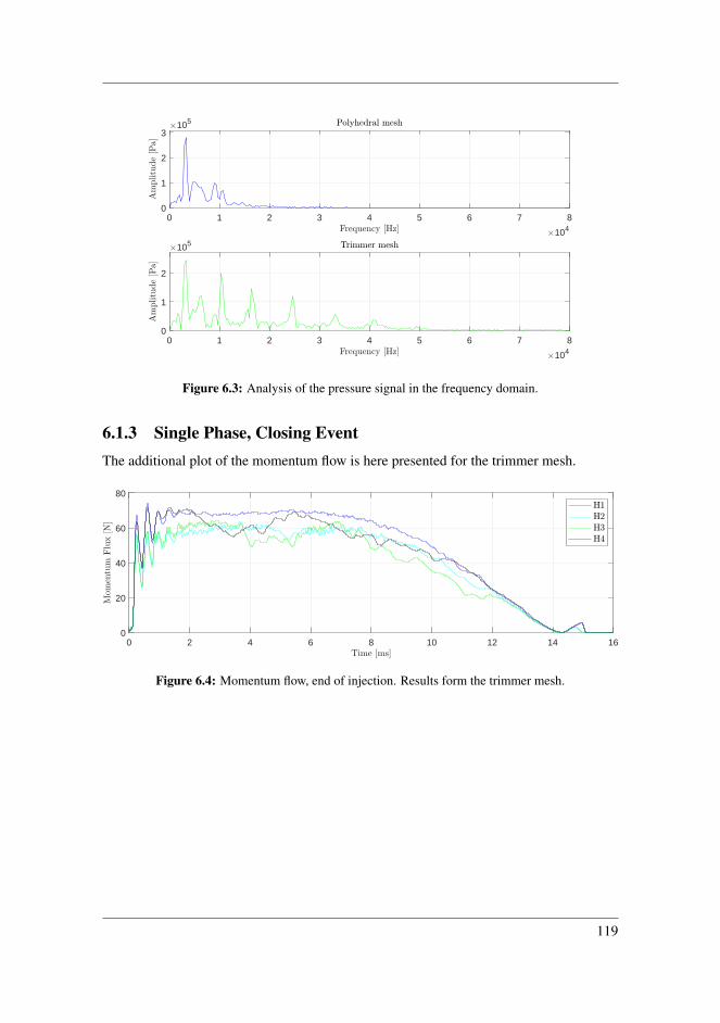
0 1 2 3 4 5 6 7 8

104

0

1

2

310

5

0 1 2 3 4 5 6 7 8

104

0

1

2

105

Figure 6.3: Analysis of the pressure signal in the frequency domain.

6.1.3 Single Phase, Closing EventThe additional plot of the momentum flow is here presented for the trimmer mesh.

0 2 4 6 8 10 12 14 16

0

20

40

60

80

Figure 6.4: Momentum flow, end of injection. Results form the trimmer mesh.

119

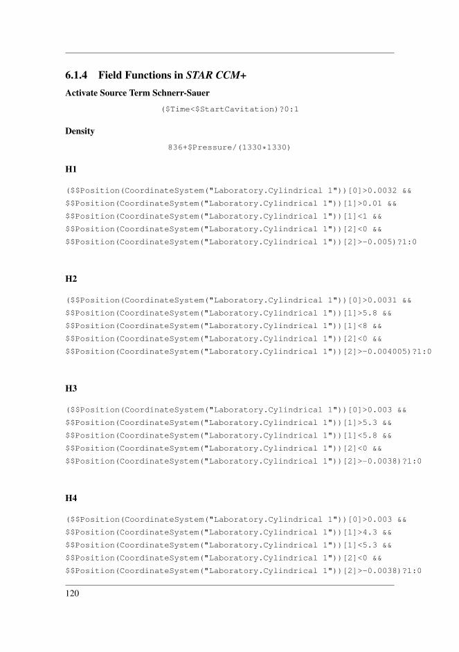
6.1.4 Field Functions in STAR CCM+Activate Source Term Schnerr-Sauer

($Time<$StartCavitation)?0:1

Density

836+$Pressure/(1330*1330)

H1

($$Position(CoordinateSystem("Laboratory.Cylindrical 1"))[0]>0.0032 &&

$$Position(CoordinateSystem("Laboratory.Cylindrical 1"))[1]>0.01 &&

$$Position(CoordinateSystem("Laboratory.Cylindrical 1"))[1]<1 &&

$$Position(CoordinateSystem("Laboratory.Cylindrical 1"))[2]<0 &&

$$Position(CoordinateSystem("Laboratory.Cylindrical 1"))[2]>-0.005)?1:0

H2

($$Position(CoordinateSystem("Laboratory.Cylindrical 1"))[0]>0.0031 &&

$$Position(CoordinateSystem("Laboratory.Cylindrical 1"))[1]>5.8 &&

$$Position(CoordinateSystem("Laboratory.Cylindrical 1"))[1]<8 &&

$$Position(CoordinateSystem("Laboratory.Cylindrical 1"))[2]<0 &&

$$Position(CoordinateSystem("Laboratory.Cylindrical 1"))[2]>-0.004005)?1:0

H3

($$Position(CoordinateSystem("Laboratory.Cylindrical 1"))[0]>0.003 &&

$$Position(CoordinateSystem("Laboratory.Cylindrical 1"))[1]>5.3 &&

$$Position(CoordinateSystem("Laboratory.Cylindrical 1"))[1]<5.8 &&

$$Position(CoordinateSystem("Laboratory.Cylindrical 1"))[2]<0 &&

$$Position(CoordinateSystem("Laboratory.Cylindrical 1"))[2]>-0.0038)?1:0

H4

($$Position(CoordinateSystem("Laboratory.Cylindrical 1"))[0]>0.003 &&

$$Position(CoordinateSystem("Laboratory.Cylindrical 1"))[1]>4.3 &&

$$Position(CoordinateSystem("Laboratory.Cylindrical 1"))[1]<5.3 &&

$$Position(CoordinateSystem("Laboratory.Cylindrical 1"))[2]<0 &&

$$Position(CoordinateSystem("Laboratory.Cylindrical 1"))[2]>-0.0038)?1:0

120

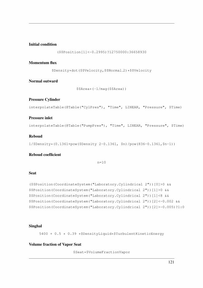
Initial condition

($$Position[1]<-0.2995)?12750000:36658930

Momentum flux

$Density*dot($$Velocity,$$Normal 2)*$$Velocity

Normal outward

$$Area*(-1/mag($$Area))

Pressure Cylinder

interpolateTable(@Table("CylPres"), "Time", LINEAR, "Pressure", $Time)

Pressure inlet

interpolateTable(@Table("PumpPres"), "Time", LINEAR, "Pressure", $Time)

Reboud

1/$Density*(0.1361+pow($Density 2-0.1361, $n)/pow(836-0.1361,$n-1))

Reboud coefficient

n=10

Seat

($$Position(CoordinateSystem("Laboratory.Cylindrical 2"))[0]>0 &&

$$Position(CoordinateSystem("Laboratory.Cylindrical 2"))[1]>0 &&

$$Position(CoordinateSystem("Laboratory.Cylindrical 2"))[1]<8 &&

$$Position(CoordinateSystem("Laboratory.Cylindrical 2"))[2]<-0.002 &&

$$Position(CoordinateSystem("Laboratory.Cylindrical 2"))[2]>-0.005)?1:0

Singhal

5400 + 0.5 * 0.39 *$DensityLiquid*$TurbulentKineticEnergy

Volume fraction of Vapor Seat

$Seat*$VolumeFractionVapor

121

Volume fraction of Vapor H1

$H1*$VolumeFractionVapor

Volume fraction of Vapor H2

$H2*$VolumeFractionVapor

Volume fraction of Vapor H3

$H3*$VolumeFractionVapor

Volume fraction of Vapor H4

$H4*$VolumeFractionVapor

122

The study of this Master thesis allows to develop and tune-up a numerical CFD model for the in-nozzle flow during the opening and closing of the fuel valve. The lack of the experimental data required the need of taking a step back and validate the model with two test cases: the periodic cavitating flow in a converging-diverging nozzle and the single phase flow inside the injector. After having shown a satisfying agreement with the reference data, the Rayleigh-Plesset cavitation model is implemented in the CFD model of the injector and the supercavitation regime is observed. The transient simulation demonstrated that both the mechanisms known as hydrodynamic and string cavitation appear in operative conditions.

Technical University of DenmarkDTU MEKSection of Fluid Mechanics, Costal and Maritime Engineering

Nils Koppels Alle, Building 403

2800 Kgs. Lyngby

Denmark

www.mek.dtu.dk

Università degli Studi di PadovaDepartment of Industrial EngineeringMechanical Engineering

via 8 Febbraio, 2

35122 Padova

Italy

www.im.dii.unipd.it