nrel/sce high penetration pv integration project: …€¢ lab testing of advanced pv inverter...

NREL is a national laboratory of the U.S. Department of Energy Office of Energy Efficiency & Renewable Energy Operated by the Alliance for Sustainable Energy, LLC This report is available at no cost from the National Renewable Energy Laboratory (NREL) at www.nrel.gov/publications.

Contract No. DE-AC36-08GO28308

NREL/SCE High Penetration PV Integration Project: FY13 Annual Report Barry A. Mather National Renewable Energy Laboratory

Sunil Shah Southern California Edison

Benjamin L. Norris and John H. Dise Clean Power Research

Li Yu, Dominic Paradis, and Farid Katiraei Quanta Technology

Richard Seguin, David Costyk, Jeremy Woyak, Jaesung Jung, Kevin Russell, and Robert Broadwater Electrical Distribution Design, Inc.

Technical Report NREL/TP-5D00-61269 June 2014

NREL is a national laboratory of the U.S. Department of Energy Office of Energy Efficiency & Renewable Energy Operated by the Alliance for Sustainable Energy, LLC This report is available at no cost from the National Renewable Energy Laboratory (NREL) at www.nrel.gov/publications.

Contract No. DE-AC36-08GO28308

National Renewable Energy Laboratory 15013 Denver West Parkway Golden, CO 80401 303-275-3000 • www.nrel.gov

NREL/SCE High Penetration PV Integration Project: FY13 Annual Report Barry A. Mather National Renewable Energy Laboratory

Sunil Shah Southern California Edison

Benjamin L. Norris and John H. Dise Clean Power Research

Li Yu, Dominic Paradis, and Farid Katiraei Quanta Technology

Richard Seguin, David Costyk, Jeremy Woyak, Jaesung Jung, Kevin Russell, and Robert Broadwater Electrical Distribution Design, Inc.

Prepared under Task No. SS12.2910

Technical Report NREL/TP-5D00-61269 June 2014

NOTICE

This report was prepared as an account of work sponsored by an agency of the United States government. Neither the United States government nor any agency thereof, nor any of their employees, makes any warranty, express or implied, or assumes any legal liability or responsibility for the accuracy, completeness, or usefulness of any information, apparatus, product, or process disclosed, or represents that its use would not infringe privately owned rights. Reference herein to any specific commercial product, process, or service by trade name, trademark, manufacturer, or otherwise does not necessarily constitute or imply its endorsement, recommendation, or favoring by the United States government or any agency thereof. The views and opinions of authors expressed herein do not necessarily state or reflect those of the United States government or any agency thereof.

This report is available at no cost from the National Renewable Energy Laboratory (NREL) at www.nrel.gov/publications.

Available electronically at http://www.osti.gov/scitech

Available for a processing fee to U.S. Department of Energy and its contractors, in paper, from:

U.S. Department of Energy Office of Scientific and Technical Information P.O. Box 62 Oak Ridge, TN 37831-0062 phone: 865.576.8401 fax: 865.576.5728 email: mailto:[email protected]

Available for sale to the public, in paper, from:

U.S. Department of Commerce National Technical Information Service 5285 Port Royal Road Springfield, VA 22161 phone: 800.553.6847 fax: 703.605.6900 email: [email protected] online ordering: http://www.ntis.gov/help/ordermethods.aspx

Cover Photos: (left to right) photo by Pat Corkery, NREL 16416, photo from SunEdison, NREL 17423, photo by Pat Corkery, NREL 16560, photo by Dennis Schroeder, NREL 17613, photo by Dean Armstrong, NREL 17436, photo by Pat Corkery, NREL 17721.

http://www.osti.gov/scitech

mailto:[email protected]

mailto:[email protected]

http://www.ntis.gov/help/ordermethods.aspx

Acknowledgments This work was supported by the U.S. Department of Energy under Contract No. DOE-EE0002061 with the National Renewable Energy Laboratory and by the California Public Utility Commission (CPUC) through the California Solar Initiative (CSI) Research, Development, Demonstration and Deployment (RD&D) Program managed by Itron. Additionally, the project would like to thank Southern California Edison (SCE) and its constituent staff for their willing participation in the project, and the insight they provided on the issues resulting from the integration of high penetration PV on the distribution system, techniques to assess the impact of PV integration, and methods for PV impact mitigation.

iii


Table of Contents 1 Introduction ........................................................................................................................................... 1 2 High-Resolution PV Power Modeling for Distribution Circuit Analysis .......................................... 3 3 PV Inverter Reactive Power Controls in OpenDSS for High Penetration Scenarios – Reduced

IEEE 8500 Node Feeder with PV ........................................................................................................ 28 4 Methods for Performing High Penetration PV Studies ................................................................. 106 5 PV Interconnection Assessment for Fontana Circuit ................................................................... 145 6 PV Interconnection Assessment for Porterville Circuit ............................................................... 157 7 PV Interconnection Assessment for Palmdale Circuit ................................................................. 187

iv


1 Introduction In 2010, the National Renewable Energy Laboratory (NREL), Southern California Edison (SCE), Quanta Technology, Satcon Technology Corporation, Electrical Distribution Design (EDD), and Clean Power Research (CPR) teamed to analyze the impacts of high penetration levels of photovoltaic (PV) systems interconnected onto the SCE distribution system. This project was designed specifically to benefit from the experience that SCE and the project team would gain during the installation of 500 megawatts (MW) of utility-scale PV systems (with 1–5 MW typical ratings) starting in 2010 and completing in 2015 within SCE’s service territory through a program approved by the California Public Utility Commission (CPUC). This report provides the findings of the research completed under the project to date.

Research objectives of this project include:

• Development of distribution and PV system models required to evaluate the impacts of high penetration PV

• Identification and development of the necessary distribution system studies and analysis appropriate for determining the impacts of high penetration PV

• Development of high penetration PV impact mitigation strategies in the form of advanced inverter functions to enable high penetration PV interconnection

• Lab testing of advanced PV inverter functions

• Field testing of advanced PV inverter functions. The contents of this report address the following topics:

1. PV system power modeling, based on remote sensing data, for developing high spatial and temporal resolution PV power datasets required for PV impact assessment of plants that have not yet been interconnected or are not instrumented;

2. Development of a quasi-static time-series distribution simulation environment for evaluating the performance of potential PV mitigation techniques using advanced PV inverter functionality and the potential interaction of different reactive power control techniques in the interconnected PV inverters on a single distribution system;

3. Methodology for performing high penetration PV integration studies that uses salient distribution circuit operating points (minimum load, maximum generation, etc.) as a proxy for a full year's worth of data and simulation; and

4. Implementation of the high penetration PV impact assessment methodology proposed above on the three SCE study circuits: Fontana, Porterville, and Palmdale, including an analysis and recommendation for how to use reactive power control functionality of the PV system’s inverters to mitigate the impacts of high penetration PV integration.

Section 2 of this report describes the development of high temporal and spatial PV plant output data on a 1-minute timescale for 1 km x 1 km grids. The techniques outlined in this section include the application of cloud motion vector analysis for developing higher temporal resolution data from available remote-sensing-based irradiance data (e.g., repurposed satellite-based weather data). The performance of these techniques is evaluated and specific issues with the

1


developed method are discussed. Results from a PV system located on one of the SCE study circuits are presented as an example of the application of the developed techniques.

The analysis discussed in Section 3 of this report details the findings of a study undertaken as part of this project to model and evaluate the effects of advanced-functionality inverters. First, the ability to model advanced, time-dependent PV inverter controls, such as voltage droop control, was implemented within the framework of quasi-static time-series analysis. Then, a number of interesting possible PV operating scenarios were evaluated to investigate how specific advanced PV inverter functionalities would perform. This section contains an explanation of how to implement a time-dependent PV inverter controller within the OpenDSS quasi-static time-series simulation framework. Results from a number of PV deployment scenarios are presented, using the developed time-dependent PV inverter models and realistic time-series data for PV system operation and distribution system loading and automatic voltage regulation equipment control actions. For these scenarios the IEEE 8500 node test feeder is used for analysis, as it contains an assortment of all the automatic voltage regulation equipment used by U.S. utilities.

Section 4 provides a detailed, step-by-step method for completing a high penetration PV integration study using utility-grade distribution system analysis tools such as EDD's Distributed Engineering Workstation (DEW). The method described to determine the impact of an interconnected high penetration PV system uses salient days of the year as a proxy for the overall impact of the interconnected PV system over a year, or multiple years of operation. This greatly reduces the amount of data required to perform the analysis and also reduces the computational resources necessary. The Fontana circuit is used as an example circuit in this section to show how PV impacts are assessed in the proposed methodology.

Using the PV impact assessment methodology presented in Section 4, Sections 5, 6, and 7 develop PV mitigation strategies and recommended settings for the Fontana, Porterville, and Palmdale SCE study circuits, respectively. Each circuit experiences a different set of PV-related impacts, and thus the PV impact assessments reveal slightly different strategies for mitigation. However, the PV inverter settings that are recommended for implementation to minimize the distribution system-level impacts of the high penetration PV integration are very similar because the PV mitigation strategies were limited to off-unity power factor operation in order to facilitate field demonstrations. Sections 5, 6, and 7 also show that such simple mitigation strategies are quite effective in mitigating the voltage-related impacts of high penetration PV integration, reducing voltage impacts on the distribution circuit by roughly 50%.

In the final year of the project, field demonstrations of using the recommended constant power factor mitigating strategies determined in Sections 5, 6, and 7 will be completed. Furthermore, the research and testing results collected during the entire project will be compiled into a “High Penetration PV Integration Handbook” for use by distribution utility engineers facing the challenges of high penetration PV interconnections.

2


2 High-Resolution PV Power Modeling for Distribution Circuit Analysis

3


Acknowledgements The authors wish to express appreciation to David Chalmers for implementing the 1-minute SolarAnywhere resolution, and to Phil Gruenhagen for creating the user interface to build systems and access the simulation service.

4


Executive Summary NREL contracted with Clean Power Research to provide 1-minute simulation datasets of PV systems located at three high penetration distribution feeders in the service territory of SCE: Porterville, Palmdale, and Fontana, California. The resulting PV simulations will be used to separately model the electrical circuits to determine the impacts of PV on circuit operations.

The 1-minute simulations incorporate satellite-derived irradiance data with a spatial resolution of nominally 1 km x 1 km and a temporal resolution of 30 minutes. The spatial resolution is the highest available through existing satellite imagery, and is shown in Figure ES-1 for the Porterville site, which also shows the modeled PV system.

To obtain the 1-minute data, inter-image interpolations are generated with a “cloud motion vector” method by translating the previous image over time using wind speed and direction. The resulting irradiance data are fed into a PV simulation model to estimate power output.

Figure ES-1. Satellite resolution at Porterville.

PV System

5


An example of the 1-minute data is shown for Fontana in Figure ES-2 for the day having the highest variability of 2011: May 29. Of greatest interest is the highest variability observed on the distribution line, so additional analysis of ramp rates was warranted.

As shown in Figure ES-3, the number of significant ramping events is very small, but the magnitude of the highest events is significant. The number of ramping events higher than 50% of PV system rated output per minute is taken as a metric of “significant” ramping, and this is shown for the Fontana site to be 37 events per year. The highest such event is shown in Figure ES-4 with an increase in PV output (caused by a departing cloud) of 2.20 MW per minute, or 75% of the system's rated output.

Through methods such as the one described in this report and demonstrated through the datasets delivered under this project, utility engineers will be able to better predict the impacts of high penetration PV on their distribution circuits.

Figure ES-2. Highest variability day at Fontana in 2011 (May 29).

6


Figure ES-3. Ramp rate duration curve at Fontana, 2011.

Figure ES-4. Maximum ramping event at Fontana, 2011.

7


Table of Contents Executive Summary .................................................................................................................................... 5 List of Figures ............................................................................................................................................. 8 List of Tables ............................................................................................................................................... 9 Background ............................................................................................................................................... 10 Introduction: Three High Penetration Study Feeders ............................................................................ 11 Methods...................................................................................................................................................... 12

Satellite Images .................................................................................................................................... 12 Cloud Motion Vector Method .............................................................................................................. 12 PV Simulations ..................................................................................................................................... 12

Delivered Datasets .................................................................................................................................... 14 1-Minute Production Data .................................................................................................................... 14 Hourly Irradiance and Temperature Data ............................................................................................. 14

Data Validation .......................................................................................................................................... 14 CAISO Stations .................................................................................................................................... 15 SMUD Stations ..................................................................................................................................... 15 Additional Comparisons to Ground Sensors ........................................................................................ 16

Analysis...................................................................................................................................................... 17 Missing Data ......................................................................................................................................... 17 Variability ............................................................................................................................................. 18

Appendix 1: Fontana (Study Feeder 1) ................................................................................................... 22 Appendix 2: Porterville (Study Feeder 2) ................................................................................................ 24 Appendix 3: Palmdale (Study Feeder 3) .................................................................................................. 26

List of Figures

Figure ES-1. Satellite resolution at Porterville. ........................................................................................ 5 Figure ES-2. Highest variability day at Fontana in 2011 (May 29). ......................................................... 6 Figure ES-3. Ramp rate duration curve at Fontana, 2011. ...................................................................... 7 Figure ES-4. Maximum ramping event at Fontana, 2011. ........................................................................ 7 Figure 1. Study feeder locations and SCE service territory. Photo from Google Earth ...................... 11 Figure 2. Average %MAE of four CAISO locations versus time interval of comparison. .................. 15 Figure 3. Average %MAE versus time interval of comparison for more than 60 locations in SMUD

territory. ............................................................................................................................................... 16 Figure 4. %MAE versus time interval of comparison for the ISIS station in Hanford, California. ..... 16 Figure 5. Missing data at Fontana, February 24, 2011, from 13:29 to 13:58. ....................................... 17 Figure 6. GOES-west satellite image, July 24, 2011 (21:30:00 UTC), showing error streak. .............. 18 Figure 7. Highest variability day at Fontana in 2011 (May 29). .............................................................. 19 Figure 8. Absolute 1-minute ramp rates at Fontana, 2011, for every minute of the year. ................. 19 Figure 9. Ramp rate duration curve at Fontana, 2011. .......................................................................... 20 Figure 10. Highest 100 ramp rates at Fontana, 2011. ............................................................................ 20 Figure 11. Maximum ramp event at Fontana, 2011 (2.20 MW/min). ..................................................... 21 Figure 12. Fontana PV system. ................................................................................................................ 22 Figure 13. Satellite resolution at Fontana. .............................................................................................. 22 Figure 14. Porterville PV system. ............................................................................................................. 24 Figure 15. Satellite resolution at Porterville. .......................................................................................... 24 Figure 16. Palmdale PV system. .............................................................................................................. 26 Figure 17. Satellite resolution at Palmdale. ............................................................................................ 26

8


List of Tables Table 1. Fontana Ramping Statistics, 2011 ............................................................................................ 21 Table 2. Specifications for Fontana ......................................................................................................... 23 Table 3. Fontana Ramping Statistics, 2011 ............................................................................................. 23 Table 4. Specifications for Porterville ..................................................................................................... 25 Table 5. Porterville Ramping Statistics, 2011 ......................................................................................... 25 Table 6. Palmdale Ramping Statistics, 2011........................................................................................... 27

9


Background SolarAnywhere is the premier solar irradiance time-series source for all locations within the continental United States, Hawaii, Mexico, the Caribbean, and parts of Canada. Irradiance estimates are generated using National Oceanic and Atmospheric Administration (NOAA) Geostationary Operational Environmental Satellites (GOES) visible satellite images processed using the most current algorithms developed by Dr. Richard Perez at the University at Albany (SUNY). These algorithms extract cloud indices from the satellite's visible channel using a self-calibrating feedback process that is capable of adjusting for arbitrary ground surfaces. The cloud indices are used to modulate physically based radiative transfer models describing localized clear sky climatology. SolarAnywhere irradiance estimates have several advantages over ground-based measurements, including longer histories, lower costs, faster time to market, and the ability to directly produce solar power and variability forecasts.

Clean Power Research works with Dr. Perez and SUNY to capture the latest advances in methodology and improvements to consistently provide the highest-quality estimates across the widest variety of site conditions. The models have, to date, provided irradiance estimates for specific sites hourly on a 10 km x 10 km (“Standard Resolution”) basis or half-hourly on a 1 km x 1 km (“Enhanced Resolution”) basis that extend from 1998 to the present hour and also include a seven-day look-ahead forecast. Recent research advances have enabled the creation of 1-minute interpolated data from the 1-km images.

These new data, with a resolution of 1 km x 1 km x 1 minute, are referred to as “High Resolution,” and under this project are used as the key input to 1-minute PV simulations.

Dr. Perez’s model was originally verified by NREL against 31 U.S. locations with varying climates before being selected to create updates of the U.S. National Solar Radiation Data Base (NSRDB). This independent validation1 found that the average hourly mean bias error of the model was 0.2 W/m2 for global horizontal irradiance (GHI) and 16.5 W/m2 for direct normal irradiance (DNI). The latest version of the model in Standard Resolution continues to be used to provide updates to the NSRDB, as well as serve as the resource database of choice for major energy agencies, such as the California Solar Initiative (CSI) and New York State Research and Development Authority (NYSERDA).

One-minute irradiance data, such as SolarAnywhere High Resolution, and the associated PV simulation model, could enable utility engineers to model PV resources on the electric distribution system. With the temporal resolution corresponding to the approximate timeframe of distribution voltage regulators, the data could be used to determine impacts of PV on distribution operations.

1 Wilcox, S., R. Perez, R. George, W. Marion, D. Meyers, D. Renné, A. DeGaetano, and C. Gueymard (2005). "Progress on an Updated National Solar Radiation Data Base for the United States." Proc. ISES World Congress, Orlando, FL.

10


Introduction: Three High Penetration Study Feeders Under the current project, NREL has contracted with Clean Power Research to provide PV simulation support for three high penetration distribution feeders under study in the service territory of SCE. The three study feeders, located in Porterville, Palmdale, and Fontana, California, are mapped in Figure 1.

Figure 1. Study feeder locations and SCE service territory. Photo from Google Earth

At each location, a large PV system is interconnected to the SCE feeder. Using the High Resolution irradiance data, ambient temperature data, PV plant specifications, and PV simulation methods, 1-minute timescale PV power generation data can be calculated. The datasets can in turn be used, along with physical component and load data, as inputs into electrical circuit modeling tools. The datasets provide PV output, in MW, for each minute of 2011. This report documents the creation of these datasets and characterizes the systems in terms of ramp rates.

11


Methods SolarAnywhere High Resolution data is derived from the same satellite image processing algorithm that generates both the SolarAnywhere Standard and Enhanced Resolutions. However, the High Resolution data uses an added method of temporal interpolation between half-hourly satellite images to create minute-by-minute solar irradiance estimates in SolarAnywhere’s current geographic coverage area.

Satellite Images SolarAnywhere satellite images are processed using the most recent version of the Perez model. In general, satellite images are obtained for coverage areas in the western and eastern halves of the continental United States and Hawaii on half-hourly increments from the Space Science and Engineering Center (SSEC) at University of Wisconsin – Madison. Following image transfer, irradiance measurements are made using the Perez model by ranking pixel brightness on clear sky conditions. Half-hourly measurements of GHI and DNI are derived from the model, which is then used to calculate residual diffuse horizontal irradiance (DHI).

Cloud Motion Vector Method To generate the 1-minute irradiance measurements, SolarAnywhere first calculates a wind vector for every Standard Resolution tile using consecutive satellite images. The wind vectors are then applied to the Enhanced Resolution irradiance map to predict movement on a minute-by-minute basis. For forecasting purposes, the prediction is calculated forward up to 60 minutes. For historical generation, the prediction occurs between half-hour segments of retrieved satellite images.

PV Simulations SolarAnywhere High Resolution data can be further used to simulate PV system generation through Clean Power Research’s PV Simulator engine. PV Simulator uses a version of the PVForm model to simulate electricity production based on a set of parameters, including irradiance, wind, temperature, installation location and specifications, and equipment specifications.

The simulation process starts by passing in the location and time-series weather data to the Perez irradiance model found in SolarAnywhere. The selected weather data source provides time-series GHI, DNI, wind, and temperature data; the site location is used to define the latitude and longitude of the PV system. Using the Perez irradiance model, PVSimulator then calculates the circumsolar diffuse irradiance, isotropic diffuse, and horizon band diffuse irradiance components. These calculations start with determining the declination of the sun and equation of time. Then the solar zenith angle is calculated based on the declination of the sun, equation of time, and latitude. The airmass is then estimated as a function of the solar zenith angle. Based on these values, the Perez model then produces the circumsolar diffuse irradiance, isotropic diffuse, and horizon band diffuse irradiance components.

After the irradiance model has broken down GHI and DNI into componentized irradiance values, PVSimulator then uses the PV array geometry to calculate the plane of array irradiance (POAI). The POAI calculations begin by calculating the solar time, taking into account the local time,

12


time zone, longitude, and the previously calculated equation of time value. The solar azimuth angle is then calculated based on the zenith angle, latitude, and declination of the sun. The plane of array (POA) angle of incidence (AOI) is then calculated based on previously calculated values, taking into account the tracking capabilities of the PV system. The components of the POAI (POA beam, circumsolar diffuse, isotropic diffuse, horizon band diffuse, and reflected irradiance components) are then calculated based on the output of the Perez model in conjunction with the tilt of the PV modules, the calculated AOI, and the specified albedo of the surrounding area. The shading model then adjusts the previously calculated POAI to account for shading as a consequence of obstructions as well as row-on-row shading.

The POAI values are then passed into the selected power output model in order to estimate the energy production of the PV system. Before calculating estimated energy production, the temperature of the PV modules is estimated based on the POAI as well the time-series wind speed and ambient temperature data provided by the weather data source. Then the 1-minute power output of the PV system is calculated based on the estimated PV module temperature and POAI along with model parameters defining the behavioral characteristics of the PV system as provided in the PV system specification. The model parameters depend on the selected power output model, but, for example, in the case of PVForm the model parameters will consist of quantities such as the module performance test conditions (PTC) rating and efficiency reduction per degree Celsius, as well as inverter average efficiency and kW AC rating.

Once all this processing has been completed, the primary output of the simulation is then the estimated 1-minute power of the PV system. In addition to this, each stage of processing may also output 1-minute intermediate calculated results (such as POA and AOI).

13


Delivered Datasets 1-Minute Production Data Using the methods previously described, four datasets of 1-minute PV system power generation were prepared and delivered2 to NREL. Data files included four columns:

• Time stamp, start of interval

• Time stamp, end of interval

• Power (MW)

• Observation Type. Observation Type3 includes keys (A) “Archived,” (D) “Day,” (N) “Night,” and (M) “Missing.”

Hourly Irradiance and Temperature Data SolarAnywhere Standard Resolution (version 2.2) data were also provided for Fontana and Porterville, including hourly measurements of GHI, DNI, DHI, wind speed, and temperature. These data were used for related circuit modeling work.

Data were provided for these two locations, between the dates of January 1, 2002, through December 31, 2011. The 10-km gridded tiles centered at 34.05 north, 117.55 west, and 36.05 north, 119.05 west, were selected for the Fontana and Porterville sites, respectively.

Data Validation Following the implementation of 1-minute data in SolarAnywhere, studies to validate the model accuracy were conducted. In collaboration with California ISO (CAISO) and Sacramento Municipal Utility District (SMUD), 1-minute data accuracy was validated against high-accuracy, well-maintained ground-mounted irradiance sensors throughout the state of California. This validation work falls outside the scope of the current project, but is provided here for completeness.

2 Results were prepared on March 5, 2013, and made available on an FTP server. 3 All data were marked as (A) archived because 2011 contains only historical data older than one month. A complete list of observation types is available at www.solaranywhere.com.

14


http://www.solaranywhere.com/

CAISO Stations To validate the SolarAnywhere 1-minute High Resolution GHI calculations, results were compared against data from four CAISO ground stations—with two sensors at each station—to determine the relative mean absolute error (%MAE) for each station. As seen in Figure 2, the average %MAE for the four stations decreases from roughly 10% at a 1-minute interval of comparison to a range of 2%–2.5% when compared annually. Additionally, the black baseline marked “Ground (Station 2)” represents the relative ground measurement error between the primary and secondary ground sensor at each location. Having two co-located ground measurement devices also accounts for the shaded green region reflecting the %MAE, as SolarAnywhere 1-minute data were compared to each of the two ground sensors, thus creating the high and low accuracy boundaries.

Figure 2. Average %MAE of four CAISO locations versus time interval of comparison.

SMUD Stations Additional validation of the SolarAnywhere High Resolution model was conducted using a network of more than 60 pole-mounted pyranometers maintained by SMUD throughout their service territory. GHI measurements from the ground stations were each compared with the corresponding SolarAnywhere High Resolution location. Figure 3 represents the %MAE average for all stations included, as a function of the time interval of comparison. The red curve represents the accuracy of the High Resolution data. The blue and green lines represent accuracy measurements of Enhanced and Standard Resolution, respectively. The result comparing SolarAnywhere High Resolution to the SMUD ground sensor GHI measurements resulted in a similar accuracy assessment, with 1-minute SolarAnywhere data falling within roughly 7% of %MAE of the corresponding ground measurement and with an overall bias of plus or minus 1%–2%.

15


Figure 3. Average %MAE versus time interval of comparison for more than 60 locations in SMUD

territory.

Additional Comparisons to Ground Sensors An accuracy summary of SolarAnywhere High Resolution data compared to the ground-collected GHI data from the Hanford Integrated Surface Irradiance Study (ISIS) station for the year 2011 is presented in Figure 4.

Figure 4. %MAE versus time interval of comparison for the ISIS station in Hanford, California.

16


Analysis The description of the analysis that follows uses only the Fontana data for simplicity in describing the process. Results for each of the locations are shown in the Appendices.

Missing Data Ramp rates (defined as the absolute change of power output4 per unit time) were calculated for every minute of the year. By inspection, it was discovered that some of the highest ramp rates were based on data that appeared to be invalid. This required further investigation.

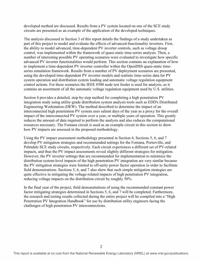
Figure 5 shows the Fontana 1-minute data for the day having the highest ramp rate (the “drop in power” from near full power output to zero). While this behavior is possible in practice—for example, due to an inverter malfunction resulting in complete power loss—it is not possible to see a zero output in the middle of the day due only to the presence of clouds. There is always some diffuse radiant energy available, even in the darkest of overcast days. Therefore, this data is clearly missing and should not be included in the analysis5.

Upon further investigation, the cause of this error was found to be an aberration in the raw satellite image. As shown in Figure 6, the image associated with the missing data includes a streak across the image, and Fontana happens to lie directly along the aberrant line. Therefore, in the 30-minute period following this image, the calculated 1-minute data are missing. The images taken in the half hour before and the half hour after this image were not distorted, and the missing data are confined to only this 30-minute period.

Figure 5. Missing data at Fontana, February 24, 2011, from 13:29 to 13:58.

4 For example, if the power output for one interval were 2.5 MW, and the power output for the next interval were 2.3 MW, then the change in power is -0.2 MW and the absolute change in power is 0.2 MW. Finally, as the intervals are 1 minute in duration, the ramp rate is 0.2 MW per minute. 5 The dataset includes an “M” flag in the observation type if the data are missing. The problem described here was not flagged as missing because the underlying satellite images do exist. The issues identified here resulted in removal of the selected images, hence the “M” flag would show up were the datasets to be re-generated. However, the search for such anomalies was limited to only those resulting in the highest ramp rates.

17


Figure 6. GOES-west satellite image, July 24, 2011 (21:30:00 UTC), showing error streak.

Analysis of data from each location showed similar cases of zeroed data. The search for such data was not exhaustive, and satellite images were not consulted each time. Rather, only the data affecting the highest ramp rates were identified. In each case, two or three of the highest ramp rates were identified as being caused by this problem and these data were manually excluded from the analysis. The highest ramp rates that follow for each location reflect data that appear to be correct and unrelated to missing data.

Variability Daily variability is defined as the standard deviation of the population of 1-minute ramp rates during the day, and is calculated as:

where 𝑁 is the number of minutes in each day, 𝑟 is the ramp rate for the 𝑖𝑡ℎminute, and is the average ramp rate over the day.

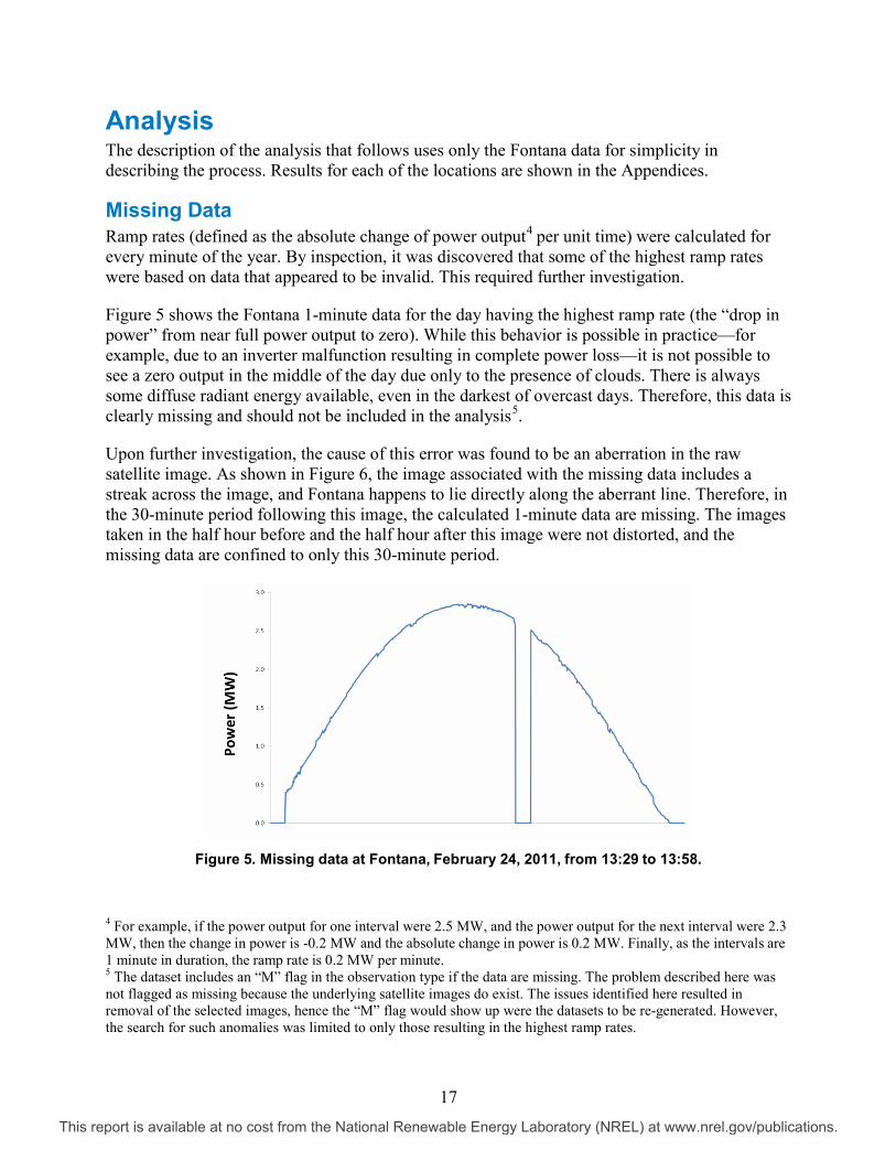
Daily variability was calculated for every day, and the day with the highest variability, May 29, is shown in Figure 7.

18


Ramp Rate Duration Curve

Figure 7. Highest variability day at Fontana in 2011 (May 29).

Figure 8 shows the ramp rates at Fontana for each of the 525,600 minutes of 2011. From this we can get a sense of the magnitude of the highest ramping events. The “normal” periods of ramping are difficult to discern, however, so this data is sorted by magnitude and presented as a “ramp rate duration curve”6 in Figure 9.

Figure 8. Absolute 1-minute ramp rates at Fontana, 2011, for every minute of the year.

6 This term is used to parallel a similar ranking of loads in electric utility planning, the “load duration curve.”

19


Figure 9. Ramp rate duration curve at Fontana, 2011.

This sorting illustrates that the number of significant ramping events is quite small. To further examine and quantify the ramping, we magnify only the top 100 minutes of the year and normalize ramping as a percent of rated PV system output. Figure 10 shows these minutes, and further defines a “high ramping region” of the curve, arbitrarily selected as covering those ramping events that correspond to an excess of 50% of PV system rating. There are 32 such high ramping events, and the largest of these is 2.20 MW per minute, or 75% of the PV system’s 2.95 MW-AC rating per minute. This event is shown in Figure 11.

Figure 10. Highest 100 ramp rates at Fontana, 2011.

20


Figure 11. Maximum ramp event at Fontana, 2011 (2.20 MW/min).

An inspection of Figure 11 also reveals an artifact of the high-resolution irradiance data generation process. With the raw image data available in half-hour intervals, the “interpolation” between two images is actually based on a given set of wind vectors and the first image corresponding to a specific time. The second image at the end of the half-hour period is not used. Hence the computations can result in a disjoint between the last minute of one period and the first minute of the next. A future improvement to the 1-minute data creation might be to use both images to ensure a smooth transition.

Finally, the ramping statistics for Fontana are summarized in Table 1. Similar ramping statistics are presented for each location in the Appendix.

Table 1. Fontana Ramping Statistics, 2011

System rating (MW) 2.95 Max. power ramp (MW per min) 2.20 Max. power ramp (% per min) 75% High ramping events (no. per year) 32

21


Appendix 1: Fontana (Study Feeder 1)

Figure 12. Fontana PV system.

Figure 13. Satellite resolution at Fontana.

22


Table 2. Specifications for Fontana

Coordinates 34.080, -117.517 Inverters Quantity: 4

Manufacturer: SatCon Technology Model: 500 kW (Model AE-500-60-PV-A) Efficiency Rating 95%

Modules Quantity: 33,700 Manufacturer: First Solar Model: 72.5W (Model FS-272) Nominal Rating (kW DC): 0.07250 PTC Rating (kW DC): 0.06980

Array Configuration Quantity: 33,700 Manufacturer: First Solar Model: 72.5W (Model FS-272) Nominal Rating (kW DC): 0.07250 PTC Rating (kW DC): 0.06980

Solar Obstructions None (Shading)

Table 3. Fontana Ramping Statistics, 2011

23


Appendix 2: Porterville (Study Feeder 2)

Figure 14. Porterville PV system.

Figure 15. Satellite resolution at Porterville.

24


Table 4. Specifications for Porterville

Coordinates 36.028738, -119.075886 Inverters Quantity: 7

Manufacturer: SatCon Technology Model: 1000 kW (Model EPP-1000-0600-32060-200X-U-x) Efficiency Rating 96.5%

Modules Quantity: 29,428 Manufacturer: Trina Solar Model: 230W (Model TSM-230PA05.10) Nominal Rating (kW DC): 0.230 PTC Rating (kW DC): 0.2089

Array Configuration Azimuth Angle: 0.000 (south) Tilt Angle: 25.000 Tracking: Fixed Array

Solar Obstructions (Shading)

None

Table 5. Porterville Ramping Statistics, 2011


25


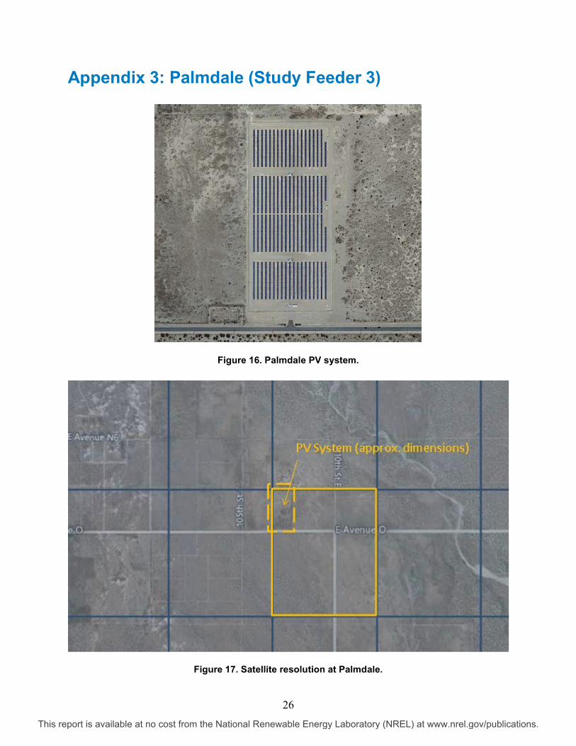
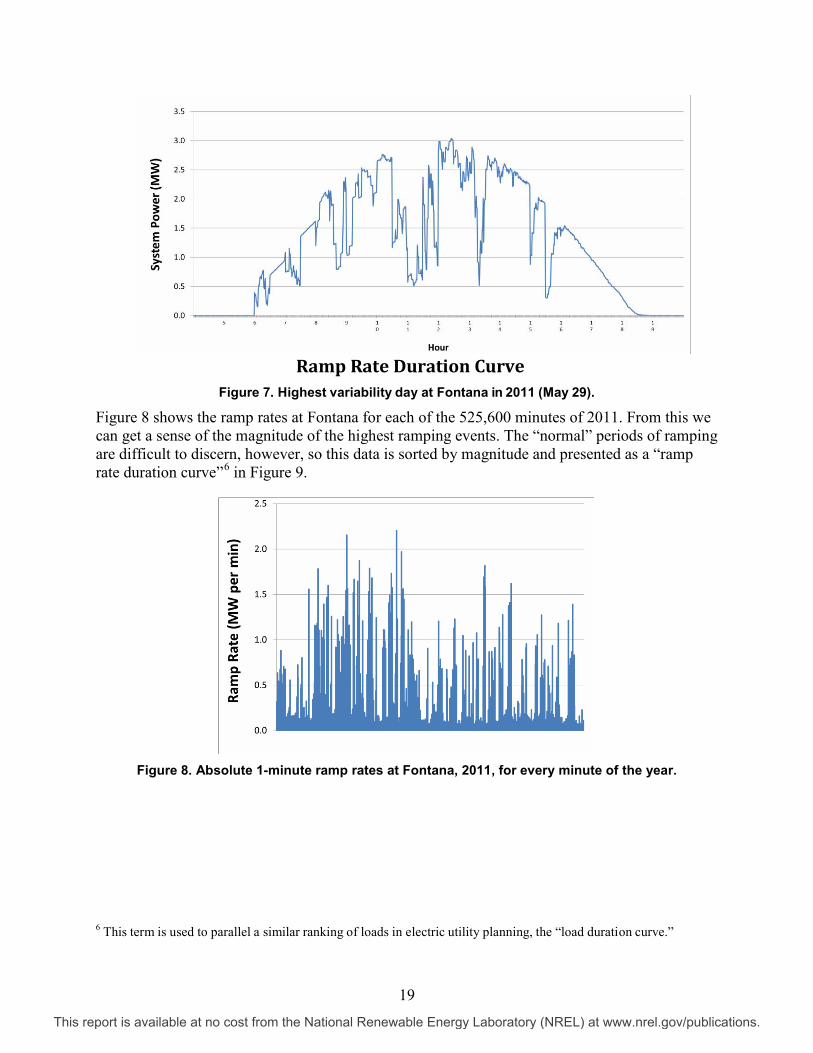
Appendix 3: Palmdale (Study Feeder 3)

Figure 16. Palmdale PV system.

Figure 17. Satellite resolution at Palmdale.

26


Table 6. Palmdale Ramping Statistics, 2011


27


3 PV Inverter Reactive Power Controls in OpenDSS for High Penetration Scenarios – Reduced IEEE 8500 Node Feeder with PV

28


Table of Contents List of Figures ........................................................................................................................................... 29 List of Tables ............................................................................................................................................. 31 Introduction ............................................................................................................................................... 33 System Layout ........................................................................................................................................... 35 Descriptions of PV Inverter Control Schemes ....................................................................................... 36

1. Power Factor Scheduling ............................................................................................................... 36 2. Reactive Power Compensation ...................................................................................................... 36 3. Dynamic Voltage Control .............................................................................................................. 36

Simulation Cases for Verification of Inverter Reactive Power Controls ............................................. 39 Simulation Including All PV with Power Factor of 0.97 and Variable Loads ..................................... 41 Simulation Including All PV Systems with Power Factor of -0.97 and Variable Loads ..................... 47 Simulation Including All PV Systems with Fixed 200 kVAr Reactive Power Generation and Variable

Loads .............................................................................................................................................. 53 Comparison Study of Simulations with 5-Second and 40-Second Time Steps .................................. 58

Comparison of No PV Case ................................................................................................................. 59 Comparison of 50% PV with PF = -0.9 at Power Factor Control Mode Case ..................................... 61 Comparison of 50% PV with PF = -0.95 at Power Factor Control Mode Case ................................... 63

Simulation Results for Inverters with Different Control Schemes ....................................................... 65 Base Case 1: Different Inverter Controls for 50% (1 MW) and 100% (2 MW) of PV Generation ..... 65 Base Case 2: Different Inverter Controls under Variable PV Profile and Variable Loads .................. 74 Base Case 3: Effect of Adding Individual PV Systems to the Feeder with Variable Profile ............... 78 Comparison Case 1: Multiple PV Systems with Different Power Factor Settings ............................... 80 Comparison Case 2: PV Systems with Different Control Strategies .................................................... 83

Summary and Conclusions ...................................................................................................................... 86 References ................................................................................................................................................. 87 Appendix A: Reduced IEEE 8500 Node Feeder Representation .......................................................... 88 Appendix B: System Parameters ............................................................................................................ 95

List of Figures Figure 18. Simplified 8500 node feeder. ................................................................................................. 35 Figure 19. Flowchart of droop control implementation. ....................................................................... 37 Figure 20. Flowchart of implemented method for calculating system profile with the nth input

profile. .................................................................................................................................................. 38 Figure 21. Effect of the different time steps on the generation profile. .............................................. 40 Figure 22. PV power generation profile used during simulation (top) and power flow at main

regulators (bottom), with all PV systems operating with a power factor of 0.97. ........................ 42 Figure 23. Real and reactive power output of phase A of PV inverter #642, all PV systems

operating with a power factor of 0.97. .............................................................................................. 42 Figure 24. Capacitor voltages and operation, all PV systems operating with a power factor of

0.97. ...................................................................................................................................................... 43 Figure 25. Voltage at LTC and LTC reaction during simulation, all PV systems operating with a

power factor of 0.97. ........................................................................................................................... 44 Figure 26. Secondary side voltage and tap changer reaction of regulator #2 during simulation, all

PV systems operating with a power factor of 0.97.......................................................................... 44 Figure 27. Secondary side voltage and tap changer reaction of regulator #3 during simulation, all

PV systems operating with a power factor of 0.97.......................................................................... 45 Figure 28. Secondary side voltage and tap changer reaction of regulator #4 during simulation, all

PV systems operating with a power factor of 0.97.......................................................................... 45 Figure 29. PV power generation profile used during simulation, and power flow downstream of the

feeder at main regulators; all PV systems operating with a power factor of -0.97. ..................... 48

29


Figure 30. Real and reactive power output of phase A of PV inverter #642; all PV systems operating with a power factor of -0.97. ............................................................................................. 49

Figure 31. Capacitor voltages and operation; all PV systems operating with a power factor of -0.97. ..................................................................................................................................................... 49

Figure 32. Voltage at LTC and LTC reaction during simulation; all PV systems operating with a power factor of -0.97. ......................................................................................................................... 50

Figure 33. Secondary side voltage and tap changer reaction of regulator #2; all PV systems operating with a power factor of -0.97. ............................................................................................. 51



Figure 36. PV power generation profile used during simulation, and power flow at main regulators; all PV systems with reactive power generation of 200 kVAr. ........................................................ 54

Figure 37. Real and reactive power output of phase A of PV inverter #642; all PV systems operating with reactive power generation of 200 kVAr. ................................................................. 54

Figure 38. Capacitor voltages and operation; all PV systems operating with reactive power generation of 200 kVAr. ..................................................................................................................... 55

Figure 39. Voltage at LTC and LTC reaction during simulation; all PV systems operating with reactive power generation of 200 kVAr. ........................................................................................... 55

Figure 40. Secondary side voltage and tap changer reaction of regulator #2 during simulation; all PV systems operating with reactive power generation of 200 kVAr. ............................................ 56



Figure 43. Energy loss during 15-minute calculation, no PV. .............................................................. 60 Figure 44. Energy loss during 15-minute calculation, 50% PV penetration with PF = -0.9. .............. 62 Figure 45. Energy loss during 15-minute calculation, 50% PV penetration with PF = -0.95. ............ 64 Figure 46. Studied system final state – Phase A voltage profile with different levels of PV

generation (fixed load, fixed 100% solar irradiance). ..................................................................... 66 Figure 47. Studied system final state – Phase B voltage profile (fixed load, fixed 100% solar

irradiance). .......................................................................................................................................... 66 Figure 48. Studied system final state – Phase C voltage profile (fixed load, fixed 100% solar

irradiance). .......................................................................................................................................... 67 Figure 49. Studied system final state – Phase A voltage profile with different power factor (fixed

load, fixed 50% solar irradiance)....................................................................................................... 67 Figure 50. Studied system final state – Phase B voltage profile with different power factor (fixed

load, fixed 50% solar irradiance)....................................................................................................... 68 Figure 51. Studied system final state – Phase C voltage profile with different power factor (fixed

load, fixed 50% solar irradiance)....................................................................................................... 68 Figure 52. Studied system final state – Phase A voltage profile with different power factor (fixed

load, fixed 100% solar irradiance)..................................................................................................... 69 Figure 53. Studied system final state – Phase B voltage profile with different power factor (fixed

load, fixed 100% solar irradiance)..................................................................................................... 69 Figure 54. Studied system final state – Phase C voltage profile with different power factor (fixed

load, fixed 100% solar irradiance)..................................................................................................... 70 Figure 55. Studied system final state – Phase A voltage profile with different droop coefficient

(fixed load, fixed 50% solar irradiance; three different droop controls generate the same voltage profile). ................................................................................................................................... 70

Figure 56. Studied system final state – Phase B voltage profile with different droop coefficient (fixed load, fixed 50% solar irradiance; three different droop controls generate the same voltage profile). ................................................................................................................................... 71

Figure 57. Studied system final state – Phase C voltage profile with different droop coefficient (fixed load, fixed 50% solar irradiance; three different droop controls generate the same voltage profile). ................................................................................................................................... 71

30


Figure 58. Studied system final state – Phase A voltage profile with different droop coefficient (fixed load, fixed 100% solar irradiance; three different droop controls generate the same voltage profile). ................................................................................................................................... 72

Figure 59. Studied system final state – Phase B voltage profile with different droop coefficient (fixed load, fixed 100% solar irradiance; three different droop controls generate the same voltage profile). ................................................................................................................................... 72

Figure 60. Studied system final state – Phase C voltage profile with different droop coefficient (fixed load, fixed 100% solar irradiance; three different droop controls generate the same voltage profile). ................................................................................................................................... 73

Figure 61. Voltage at PV POIs when PV systems operate at unity PF. ................................................ 74 Figure 62. Voltage at PV POIs when PV systems operate at PF = -0.9. ............................................... 75 Figure 63. Voltage at PV POIs when PV systems operate at PF = -0.95. ............................................. 75 Figure 64. Reactive power of each PV system for operation at 0.95 leading power factor

(absorbing). ......................................................................................................................................... 76 Figure 65. Voltage at PV POIs when PV systems operate with 5% droop control mode. ................. 76 Figure 66. Reactive power of each PV system for 5% droop control (absorbing Q). ........................ 77 Figure 67. Voltage at PV1 POI (only one PV system operates at a time). ........................................... 78 Figure 68. Voltage at PV2 POI (only one PV system operates at a time). ........................................... 78 Figure 69. Voltage at PV3 POI (only one PV system operates at a time). ........................................... 79 Figure 70. Comparison of voltages at PV POIs when PV systems use unity power factor vs. non-

unity power factors. ........................................................................................................................... 80 Figure 71. Comparison of voltages at load 3 and 6 when PVs use unity power factor vs. non-unity

power factors. ..................................................................................................................................... 81 Figure 72. Reactive power of the PV systems with non-unity power factors. .................................... 81 Figure 73. Comparison of system kWh losses when PV inverters use unity power factor vs. non-

unity power factors. ........................................................................................................................... 82 Figure 74. Comparison of voltages at PV POIs when PV systems are operating with different

control strategies................................................................................................................................ 83 Figure 75. Comparison of voltages at loads 3 and 6 when PV systems use different control

strategies. ............................................................................................................................................ 84 Figure 76. Reactive power of the PV systems for various control strategies. ................................... 84 Figure 77. Comparison of reactive power generation percentage when PV systems use different

control strategies................................................................................................................................ 85 Figure 78. Comparison of system active power losses when PV systems use different control

strategies. ............................................................................................................................................ 85 Figure 79. General layout of simplified 8500 node feeder system. ...................................................... 88 Figure 80. PV generation profile used for simulations (x-axis is time in min). ................................... 92 Figure 81. Location of the variable loads in the feeder. ........................................................................ 93 Figure 82. Profiles used for variable loads (in per unitized of rated value). ....................................... 94 List of Tables Table 7. LTC, Regulators, and Capacitors Actions for Simulation Including All PVs with Power

Factor 0.97 and All Variable Loads ................................................................................................... 41 Table 8. LTC, Regulators, and Capacitors Actions for Simulation Including All PV Systems with

Power Factor of -0.97 and All Variable Loads ................................................................................. 47 Table 9. LTC, Regulators, and Capacitors Actions for Simulation Including All PVs with Q

Commanded at 200 kVAr and All Variable Loads ........................................................................... 53 Table 10. Comparison of LTC, Voltage Regulators, and Capacitors Operations in No PV Case ..... 59 Table 11. Comparison of LTC, Voltage Regulators, and Capacitors Operations in 50% PV with PF =

-0.9 Case .............................................................................................................................................. 61 Table 12. Comparison of LTC, Voltage Regulators, and Capacitors Operations in 50% PV with PF =

0.95 Case ............................................................................................................................................. 63 Table 13. Total Loads between Feeder Source and First Branch at Node #174 ................................. 88 Table 14. Total Loads between Node #174 and #302 ............................................................................ 89 Table 15. Load Parameters....................................................................................................................... 89

31


Table 16. Transmission Line Parameters ............................................................................................... 90 Table 17. Capacitor Control Parameters ................................................................................................. 91 Table 18. LTC and Voltage Regulators Control Parameters ................................................................. 91 Table 19. Variable Loads Used During Simulations and Associated Profiles .................................... 93

32


Introduction This report outlines the results of high PV penetration impact studies completed using the OpenDSS simulation tool and a simplified version of the IEEE 8500 node feeder model. The model was previously used to study the effects of PV plant power output fluctuations on the feeder voltages and power flow [1, 2]. In the previous simulations, the reactive power output of the PV inverters was fixed to operate at unity power factor (PF). The study focused on investigation of modeling approaches for quasi-static (time-series) impact studies [2]. The modifications implemented in support of this project allow simulations with dynamically varying reactive power output of the PV inverters to manage adverse impact on feeder voltage profiles.

The PV inverters can be controlled in three different ways:

• PF scheduling: Following a PF command

• Reactive power compensation: Following a reactive power command

• Dynamic voltage control: Dynamically adjusting the voltage at a specific location on the feeder by following a voltage-reactive power (V-Q) droop control algorithm.

Detailed descriptions of three types of control schemes listed above and simulation results for the case studies listed below are provided in the following sections.

Case studies:

• Verification of Inverter Reactive Power Controls

o All PV systems operating with a variable PV profile and the same control: PF set to 0.97 and -0.97, and reactive power set to 200 kVAr. Includes variable loads.

• Comparison Study of Simulation in 5-Second Time Step and 40-Second Time Step

o No PV, and with all PV systems receiving constant 50% irradiance levels and operating with the same control: PF set to -0.9 and -0.95. Includes only fixed loads.

• Inverters with Different Control Schemes

o No PV, and with only one PV system connected operating with different, fixed irradiance levels and several inverter controls: constant PF of 1.0, -0.9, and -0.95, and droop control with coefficients of 3%, 5% and 10%. Includes only fixed loads.

o All PV systems connected and operating with a variable solar irradiance profile and the same control: constant PF of 1.0, -0.9, and -0.95, and droop control with a coefficient of 5%. Includes variable loads.

o No PV, and with only one PV system connected at a time, operating with a variable solar irradiance profile and with unity PF. Includes variable loads.

33


o All PV systems connected and operating with a variable solar irradiance profile and with different PF settings of -0.9, -0.9, and -0.95, respectively. Includes variable loads.

o All PV systems connected and operating with a variable solar irradiance profile and with different control strategies of 4% droop, -0.9 PF, and 375 kVAr, respectively. Includes variable loads.

The benchmark system selected for this study is the simplified version of the IEEE 8500 node distribution test system that was used in the previous investigation [2], and that includes three large PV facilities. The only difference in this study is the change in the PV inverter reactive power control capabilities. The PV facilities are allowed to operate with non-unity PF based on any of the three proposed control methods. A detailed benchmark description and lists of nodes and lines are provided in Appendix A.

The overall load on the feeder is well balanced between the three phases. However, the individual loads are not distributed evenly throughout the feeder, such that the power at different points on the feeder varies between the phases. The sum of the loads on each individual phase (excluding losses) is approximately 3896 kW and 279 kVAr. The PV facilities are 2 x 2 MW and 1.5 MW (5.5 MW total). PV facilities are sized in a way that power flow through regulator #3 becomes negative (i.e., reverse flow at 100% generation), yet the power flow through regulator #2 is positive.

34


System Layout The layout of the study system is shown in Figure 18; the voltage control devices, which include three regulators and four controllable capacitor banks, are highlighted, along with associated node numbers. The substation transformer also includes an on-load tap changer (OLTC). Variable loads, i.e., loads that vary as a function of time according to profiles that are described in Appendix A, are also shown.

Figure 18. Simplified 8500 node feeder.

The simulations were performed in steady state, and the voltage, reactive, and complex power were plotted at selected locations on the feeder. Two paths down the feeder were used: one from the source to node 302 and another from the source to node 719. The latter covers the branches most affected by the presence of the PV.

35


Descriptions of PV Inverter Control Schemes Three reactive power control schemes are introduced and modeled for the PV inverters in the study system, including:

1. Power Factor Scheduling In this control scheme, the PV inverter reactive power output is adjusted by following a PF command. PF can be either inductive or capacitive. The operating range for PF is limited between 0.85 inductive and 0.85 capacitive. The MVA rating of the PV inverter is calculated based on the maximum MW output of the facility (nominal active power rating) at 0.85 PF.

2. Reactive Power Compensation In this control scheme, the PV inverter generates or absorbs fixed reactive power by following a reactive power generation command. The PV inverter has been sized based on 120% of the rated active power capacity. If the MVA rating of the PV inverter is exceeded, reactive power output of the PV inverter will be automatically capped within acceptable limits without affecting active power generation.

3. Dynamic Voltage Control In this control scheme, the PV inverter can dynamically adjust the voltage at a specific location on the feeder by following a V-Q droop control algorithm. In this study, the PV inverter point of interconnection (POI) is considered as the monitoring location to determine the voltage reference point. The reactive power limits are also determined based on the PF range of 0.85 inductive to 0.85 capacitive at rated active power output.

The droop control algorithm for PV inverter reactive power output can be described by the following equations.

If voltage at the measurement point is lower than the reference value (considering a deadband), then:

∆𝑄𝑃𝑉 = (𝑉𝑚 − 𝑉𝑟𝑒𝑓 −𝐷𝑒𝑎𝑑𝑏𝑎𝑛𝑑

2) ∗ 𝐷𝑐𝑜𝑒𝑓 ∗ 𝑘𝑉𝐴𝑃𝑉 (1)

If voltage at the measurement point is higher than the reference value (considering a deadband), then:

∆𝑄𝑃𝑉 = (𝑉𝑚 − 𝑉𝑟𝑒𝑓 + 𝐷𝑒𝑎𝑑𝑏𝑎𝑛𝑑2

) ∗ 𝐷𝑐𝑜𝑒𝑓 ∗ 𝑘𝑉𝐴𝑃𝑉 (2)

𝑄𝑃𝑉 = 𝑄𝑃𝑉,𝑏𝑒𝑓𝑜𝑟𝑒 + ∆𝑄𝑃𝑉 (3)

where ∆𝑄𝑃𝑉 is the PV inverter reactive output change based on the voltage 𝑉𝑚 at measurement point, 𝑉𝑟𝑒𝑓 is the reference voltage, 𝐷𝑐𝑜𝑒𝑓 is the droop coefficient, 𝑘𝑉𝐴𝑃𝑉 is the kVA rating of PV inverter, 𝑄𝑃𝑉,𝑏𝑒𝑓𝑜𝑟𝑒 is the initial PV inverter reactive power output, and 𝑄𝑃𝑉 is the PV inverter reactive power output after droop control.

36


For the purpose of quasi-static power flow analysis with a minimum 5-second time step, it is assumed that the PV inverter controls can execute a droop control scheme and determine the next set point for reactive power in a timeframe shorter than 5 seconds. Hence, in this study it is assumed that, in a time step greater than 5 seconds, the Q adjustment through the droop control has one of the following three conditions:

5. The reactive power output of the PV inverter is re-adjusted such that the voltage at the measurement point is within the given deadband, or

6. The PV inverter PF reaches the given upper or lower thresholds, and therefore additional Q adjustment is not possible, or

7. The PV inverter kVA output reaches its upper kVA limit, and additional Q adjustment is not possible (priority is given to maximum active power output).

Based on the above three conditions, as long as the PV inverter PF and capacity limits are not exceeded, a different droop coefficient does not produce different voltage regulation results.

The overall droop control algorithm used in this study is illustrated in the following flowchart, which is executed within a single time step.

Figure 19. Flowchart of droop control implementation.

37


From Figure 19, it can be seen that, for completing one full control loop based on the voltage-droop scheme, several iterations of the load-flow calculation are used to update system values (including voltage profile, power losses, etc.) until the conditions are met. The number of iterations of the algorithm described in Figure 19 depends on the droop coefficient, voltage deviation at the measurement point, selected reference voltage, and deadband. In addition to droop control calculations, the load flow calculation incorporates changes in the input profiles, such as solar irradiance profile and load profile (if variable load is selected), based on the given resolution and selected time step for the studies.

For situations where quasi-static time-series analysis is attempted with PV inverters implementing droop control, the load flow solution with “ControlMode=TIME” provided by OpenDSS is no longer suitable for this study. The load flow calculation in OpenDSS represents system status based on a pre-set fixed time step. It does not have timing logic for PV inverter droop control, only for time-based control logic of the load tap changer (LTC), voltage regulators, and capacitors.

Hence, a time-sequence load flow method is implemented for this study that uses OpenDSS strictly as a load flow calculation engine, and implements all control logic for the PV inverter, LTC, voltage regulator, and capacitor outside of OpenDSS. The flowchart of the implemented method for calculating system profile for the nth point of the input profile is shown in Figure 20.

Figure 20. Flowchart of implemented method for calculating system profile with the nth input

profile.

38


Simulation Cases for Verification of Inverter Reactive Power Controls Several case studies were performed to verify the three reactive power control methods described above for PV inverters. The studies consider variable load and PV profiles, as described in Appendix A.

Different time steps are used for the simulation to study their effects on the results. The time steps selected for the first simulations were 5, 10, 15, 30, 40, and 50 seconds. The 5-second time step was used to generate results sufficiently precise to be comparable with PSCAD. The intervals were then increased to determine the effect of larger time steps on the results. For time steps equal to and less than 15 seconds, the simulation intervals are short enough to allow timely operation of the control devices, as the delays of the devices are as follows: 30 seconds for the LTC, 45 seconds for the voltage regulators, and 60 seconds for the switched capacitors. At the 10-second time step, the regulator control is effectively changed to 50 seconds, as it is impossible to apply tap control at 45-second intervals, but the deviation is small enough that it should not have much effect on the results.

Starting from the 30-second time step, the control intervals start to change. First, at 30 seconds, the control time of the regulators is changed to 60 seconds (two time steps), which is now the same as the capacitors. At 40 seconds, all the control delays are changed (to 40 seconds for the LTC, 80 seconds for the regulators, and 80 seconds for the capacitors). At 50 seconds, the time step is larger than the regulators' control time, such that if the voltage value is out of range for one step, this will cause a reaction on the next step. The reaction time is also reduced to 50 seconds compared to the previous time steps of 30 and 40 seconds where the reaction delay was 60 and 80 seconds, respectively. As such, it can be expected that the regulators will perform more operations at that time step.

Another important difference between the different time steps will be the sampling effect on the profiles, especially the generation profile of the PV systems. The profile includes multiple short peaks and dips in the power output. These may not all be represented after sampling, especially at longer time steps. As such, it can be expected that the response of the system will change. The effect of the different time steps on the actual PV profile can be seen in Figure 21.

As the figure shows, the PV profile follows the actual data quite nicely for the 5-second time step. However, starting at 10 seconds, the generation peak at t = 2 minutes has already disappeared. As this peak is very short, it may not influence the result very much, but this is still an obvious discrepancy in the profiles. Other than this difference, the profile still follows the original one relatively well. At 15-second steps, one can easily see some of the shorter-duration fluctuations disappear. At 30 seconds, most of the minor fluctuations have disappeared and the larger features are clearly distorted. At 40 seconds, any trace of the short peak at t = 2 minutes has disappeared, along with the peak at t = 10 minutes and the dip at t = 7 minutes. The same is true for the 50-second sampling; however, the peak at t = 2 minutes is still noticeable (although not nearly as large as in the 5-second case). All these differences will affect the results in ways that remain to be determined by further analysis.

39


The load profiles will not be affected as significantly as the generation profile, as the changes in these profiles are usually smaller in magnitude and longer in duration. Most changes are steps between two stable values. As such, it is not expected that the time step will have as much of an effect on the load profile simulation results.

Figure 21. Effect of the different time steps on the generation profile.

40


Simulation Including All PV with Power Factor of 0.97 and Variable Loads The first simulation case includes all the PV systems, as well as the variable loads. The PF setting of the PV inverters was 0.97 for the purpose of this simulation such that the PV inverters are introducing reactive power to the system. The time step selected for this simulation is 10 seconds. An overview of the results related to the voltage regulation devices (LTC, regulators, and capacitors) is shown in Table 7.

Table 7. LTC, Regulators, and Capacitors Actions for Simulation Including All PVs with Power Factor 0.97 and All Variable Loads

OpenDSS (10s)

Load tap changer Max 6 Min 5

# of changes 5

Regulator #2

A Max 15 Min 11

# of changes 6

B Max 13 Min 5

# of changes 10

C Max 4 Min 0

# of changes 7

Regulator #3

A Max 6 Min 3

# of changes 10

B Max 4 Min -1

# of changes 11

C Max 1 Min -2

# of changes 7

Regulator #4

A Max 7 Min 4

# of changes 7

B Max 8 Min 2

# of changes 8

C Max 4 Min -1

# of changes 8 Capacitor #1 Opening time 60s Capacitor #2 Opening time - Capacitor #4 Opening time 60s

41


The following figures show detailed results for all the simulations.

Figure 22. PV power generation profile used during simulation (top) and power flow at main

regulators (bottom), with all PV systems operating with a power factor of 0.97.

Figure 22 shows the power flow though the feeder during the simulation as well as the PV profile used. It can be seen through the reactive power flow at the source that the capacitors are opened at t = 1 minute. The influx of real and reactive power as the PV inverters come online is enough to cause the capacitors to open. It can also be seen that the reactive power follows the real power changes as well, showing that the PV inverters are generating reactive power.

Figure 23. Real and reactive power output of phase A of PV inverter #642, all PV systems

operating with a power factor of 0.97.

42


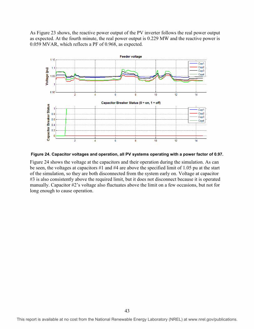
As Figure 23 shows, the reactive power output of the PV inverter follows the real power output as expected. At the fourth minute, the real power output is 0.229 MW and the reactive power is 0.059 MVAR, which reflects a PF of 0.968, as expected.

Figure 24. Capacitor voltages and operation, all PV systems operating with a power factor of 0.97.

Figure 24 shows the voltage at the capacitors and their operation during the simulation. As can be seen, the voltages at capacitors #1 and #4 are above the specified limit of 1.05 pu at the start of the simulation, so they are both disconnected from the system early on. Voltage at capacitor #3 is also consistently above the required limit, but it does not disconnect because it is operated manually. Capacitor #2’s voltage also fluctuates above the limit on a few occasions, but not for long enough to cause operation.

43


Figure 25. Voltage at LTC and LTC reaction during simulation, all PV systems operating with a

power factor of 0.97.

Figure 25 shows the reaction of the LTC to the PV in the system. Whereas the LTC did not react strongly to simulations that only included real power, the additional injection of reactive power to the system causes it to change taps much more often, although the overall range does not vary greatly.

Figure 26. Secondary side voltage and tap changer reaction of regulator #2 during simulation, all

PV systems operating with a power factor of 0.97.

44


Figure 27. Secondary side voltage and tap changer reaction of regulator #3 during simulation, all PV systems operating with a power factor of 0.97.

Figure 26 and Figure 27 show the reaction of the voltage regulators during the simulation. As these two regulators are located directly between the source and the PV inverters, they are directly affected by them. As one would expect, the voltage at the regulators was affected by the PV power generation, and required several tap changes: a few taps down initially to accommodate the increase in generation from 0% to 40%, followed by a few more around 7 minutes, when the output of the PV increases to 100%, and then taps up after the return of the generation profile to 40% power. The voltage did fluctuate far out of range on a few occasions.

Figure 28. Secondary side voltage and tap changer reaction of regulator #4 during simulation, all PV systems operating with a power factor of 0.97.

45


Figure 28 shows the reaction of voltage regulator #4, situated outside the path directly between the source and the PV systems. As one would expect, the impact at this point was less pronounced than in the case of the other two regulators, but the addition of the fluctuating loads and the voltage changes throughout the feeder still required quite a few tap changes, even this far away from the PV inverters.

As this case has shown, the OpenDSS model can be configured to follow a fixed PF command, supplying additional reactive power to the feeder.

46


Simulation Including All PV Systems with Power Factor of -0.97 and Variable Loads The second simulation performed includes all the PV systems, as well as the variable loads. The PF of the PV inverters was set to -0.97 for the purpose of this simulation such that the PV inverters are absorbing reactive power in the system. The time step selected for this simulation is 10 seconds. An overview of the results related to the voltage regulation devices (LTC, regulators, and capacitors) is shown in Table 8.

Table 8. LTC, Regulators, and Capacitors Actions for Simulation Including All PV Systems with Power Factor of -0.97 and All Variable Loads

OpenDSS (10s)


# of changes 0

Regulator #2

A Max 15 Min 11

# of changes 5

B Max 13 Min 6

# of changes 7

C Max 4 Min 0

# of changes 6

Regulator #3

A Max 6 Min 3

# of changes 8

B Max 4 Min 0

# of changes 7

C Max 2 Min -1

# of changes 5

Regulator #4

A Max 7 Min 5

# of changes 2

B Max 8 Min 3

# of changes 6

C Max 4 Min 0

# of changes 7 Capacitor #1 Opening time 340s Capacitor #2 Opening time - Capacitor #4 Opening time -

47


The following figures show detailed results for all the simulations.

Figure 29. PV power generation profile used during simulation, and power flow downstream of the

feeder at main regulators; all PV systems operating with a power factor of -0.97.

Figure 29 shows the power flow through the feeder during the simulation as well as the PV profile used. It can be seen through the reactive power flow at the source that a capacitor opens at t = 340 seconds. The effects of the influx of real power in this case are partially counteracted by the absorption of reactive power at the PV inverters such that the capacitors do not react as fast as was the case in the 0.97 PF scenario. It can also be seen that the reactive power follows the real power changes as well, showing that the PV inverters are absorbing reactive power.

48


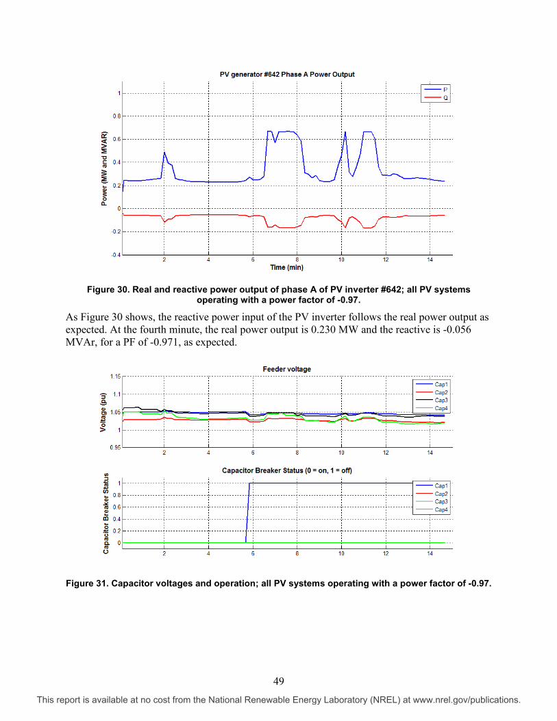
Figure 30. Real and reactive power output of phase A of PV inverter #642; all PV systems

operating with a power factor of -0.97.

As Figure 30 shows, the reactive power input of the PV inverter follows the real power output as expected. At the fourth minute, the real power output is 0.230 MW and the reactive is -0.056 MVAr, for a PF of -0.971, as expected.

Figure 31. Capacitor voltages and operation; all PV systems operating with a power factor of -0.97.

49


Figure 31 shows the voltage at the capacitors and their operation during the simulation. As can be seen, the voltage at capacitor #1 is slightly above the specified limit of 1.05 pu during the fifth minute, and it is disconnected from the system. Voltage at capacitor #3 is also above the required limit, but it does not disconnect because it is operated manually. The voltages at capacitors #2 and #4 are generally in range.

Figure 32. Voltage at LTC and LTC reaction during simulation; all PV systems operating with a

power factor of -0.97.

Figure 32 shows the reaction of the LTC to the PV in the system. In this case, because the voltage change created by the PV inverters is mitigated by their absorption of reactive power, the voltage at the feeder source remains constant enough that no operations are required.

50


Figure 33. Secondary side voltage and tap changer reaction of regulator #2; all PV systems

operating with a power factor of -0.97.

Figure 34. Secondary side voltage and tap changer reaction of regulator #3; all PV systems operating with a power factor of -0.97.

Figure 33 and Figure 34 show the reaction of the voltage regulators during the simulation. As one would expect, the voltage at the regulators was affected by the variation in PV power generation and required several tap changes, although less than required in the 0.97 PF case. A few taps down were initially required to accommodate the increase in generation from 0% to 40%, followed by a few more around 7 minutes, when the output of the PV increases to 100%, followed by taps up after the return of the generation profile to 40% power. The voltage remained in, or close to, the acceptable range throughout.

51


Figure 35. Secondary side voltage and tap changer reaction of regulator #4; all PV systems operating with a power factor of -0.97.

Figure 35 shows the reaction of voltage regulator #4, situated outside the path directly between the source and PV inverters. As one would expect, the impact at this point was less significant than in the case of the other two regulators, but the addition of the fluctuating loads and the voltage changes throughout the feeder still required quite a few tap changes.

As this case has shown, the OpenDSS model can be configured to follow a fixed PF command absorbing reactive power from the feeder.

52


Simulation Including All PV Systems with Fixed 200 kVAr Reactive Power Generation and Variable Loads The third simulation performed includes all of the PV systems, as well as the variable loads. In this case, the PV inverters are set up to generate 200 kVAr of reactive power regardless of the real power output. The time step selected for this simulation is 10 seconds. An overview of the results related to the voltage regulation devices (LTC, regulators, and capacitors) is shown in Table 9.

Table 9. LTC, Regulators, and Capacitors Actions for Simulation Including All PVs with Q Commanded at 200 kVAr and All Variable Loads

OpenDSS (10s)


# of changes 1

Regulator #2

A Max 15 Min 10

# of changes 6

B Max 13 Min 5

# of changes 9

C Max 4 Min 1

# of changes 4

Regulator #3

A Max 6 Min 3

# of changes 8

B Max 4 Min 0

# of changes 7

C Max 2 Min -1

# of changes 6

Regulator #4

A Max 7 Min 3

# of changes 6

B Max 8 Min 2

# of changes 8

C Max 4 Min 0

# of changes 6 Capacitor #1 Opening time 60s Capacitor #2 Opening time - Capacitor #4 Opening time 60s

53


The figures below show detailed results for all the simulations.

Figure 36. PV power generation profile used during simulation, and power flow at main regulators;

all PV systems with reactive power generation of 200 kVAr.

Figure 36 shows the power flow though the feeder during the simulation as well as the PV profile used. It can be seen from the reactive power flow at the source that capacitors open at about t = 1 minute. The influx of real and reactive power causes the feeder voltage to increase too quickly for the tap changers to react, which forced the capacitors to operate.

Figure 37. Real and reactive power output of phase A of PV inverter #642; all PV systems

operating with reactive power generation of 200 kVAr.

54


As Figure 37 shows, the reactive power input of the PV inverter is fixed at 66.6 kVAr (per phase), with only very small fluctuations, mainly at times when the real power fluctuates.

Figure 38. Capacitor voltages and operation; all PV systems operating with reactive power

generation of 200 kVAr.

Figure 38 shows the voltage at the capacitors and their operation during the simulation. As can be seen, the voltages at capacitors #1 and #4 are well above the specified limit of 1.05 pu from the beginning, causing both to disconnect from the system. Voltage at capacitor #3 is also above the required limit, but it does not disconnect because it is operated manually. The voltage at capacitor #2 remains in range throughout.

Figure 39. Voltage at LTC and LTC reaction during simulation; all PV systems operating with

reactive power generation of 200 kVAr.

55


Figure 39 shows the reaction of the LTC to the PV in the system. In this case, because the voltage change induced by the PV inverters is a result of changes in real power only, since the reactive power stays constant, large changes are noticed early in the simulation, but the voltages become more stable after the first minutes, as only real power changes from then on.

Figure 40. Secondary side voltage and tap changer reaction of regulator #2 during simulation; all

PV systems operating with reactive power generation of 200 kVAr.

Figure 41. Secondary side voltage and tap changer reaction of regulator #3 during simulation; all PV systems operating with reactive power generation of 200 kVAr.

56


Figure 40 and Figure 41 show the reaction of the voltage regulators during the simulation. As one could expect, the tap changes are not as numerous as for the case of a fixed PF of 0.97 after the initial disconnection of the capacitors, as the reactive power generation throughout the feeder is more stable. A few taps down were initially required to accommodate the connection of the PV inverters, followed by a few more around 7 minutes, when the output of the PV increases to 100%, followed by taps up after the return of the generation profile to 40% power. The voltages do fluctuate quite far outside the acceptable range during the generation peaks, which are not long enough for the tap changers to completely counteract them.

Figure 42. Secondary side voltage and tap changer reaction of regulator #4 during simulation; all PV systems operating with reactive power generation of 200 kVAr.

Figure 42 shows the reaction of voltage regulator #4, which is situated outside the path directly between the source and PVs. As one would expect, the impact at this point was less significant than in the case of the other two regulators, but the addition of the fluctuating loads and the voltage changes throughout the feeder still required quite a few tap changes.

As this case has shown, the OpenDSS model can be configured to follow a reactive power reference.

57


Comparison Study of Simulations with 5-Second and 40-Second Time Steps In this section, results are compared for simulations in 5-second and 40-second time steps in terms of LTC operation, voltage regulator operations, capacitor operations, and distribution system energy loss. Simulation results are shown for three scenarios: no PV, and 50% PV generation with PF control mode and PF set to -0.9 and -0.95, respectively.

Table 10, Table 11, and Table 12 show the number of LTC and voltage regulator operations and their maximum and minimum tap positions for their respective cases. Additionally, the number of capacitor operations, along with the time at which the capacitor operates, are given in the tables. Results are shown for simulation time steps of 5 and 40 seconds. While the maximum and minimum tap positions are different on only a few occasions for the case without PV, the number of changes is mostly different, and can differ by up to two counts. Results are more similar for the case with PV and PF = -0.9, but for the case with PV and PF = -0.95, the number of changes is mostly different and differ by up to three counts.

Figure 43, Figure 44, and Figure 45 show the total energy loss of the distribution system incurred during the simulation period in order to serve load on the system. Loss curves are shown for both simulation time steps investigated. For the case without PV, the differences in the results are insignificant, but for the cases with PV, the difference is more significant.

58


Comparison of No PV Case Table 10. Comparison of LTC, Voltage Regulators, and Capacitors Operations in No PV Case

Case Description No PV,

40-second time step

No PV, 5-second time

step

LTC Max Tap Position 5 5 Min Tap Position 5 5 # of changes 0 0

Regulator2

Phase A

Max Tap Position

6 6

Min Tap Position

6 6

# of changes 0 0

Phase B

Max Tap Position

4 4

Min Tap Position

2 2

# of changes 3 4

Phase C

Max Tap Position

1 2

Min Tap Position

0 0

# of changes 2 3

Regulator3

Phase A

Max Tap Position

15 15

Min Tap Position

15 15

# of changes 0 0

Phase B

Max Tap Position

13 13

Min Tap Position

8 7

# of changes 5 7

Phase C

Max Tap Position

4 4

Min Tap Position

3 2

# of changes 1 3

Regulator4 Phase

A

Max Tap Position

7 7

Min Tap Position

6 6

# of changes 1 1 Phase Max Tap 8 8

59


Case Description No PV,

40-second time step

No PV, 5-second time

step B Position

Min Tap Position

4 5

# of changes 4 3

Phase C

Max Tap Position

4 4

Min Tap Position

1 1

# of changes 5 5 Capacitor

#1 Total Servicing Time 900s 900s # of Operation 0 0

Capacitor #2

Total Servicing Time 900s 900s # of Operation 0 0

Capacitor #4


Figure 43. Energy loss during 15-minute calculation, no PV.

0 200 400 600 8000

50

100

150

200

250

Time (Second)

Ener

gy L

oss (

kWh)

No PV, 5s time stepNo PV, 40s time step

60


Comparison of 50% PV with PF = -0.9 at Power Factor Control Mode Case Table 11. Comparison of LTC, Voltage Regulators, and Capacitors Operations in 50% PV with PF =

-0.9 Case

Case Description 50% PV PF = -0.9 40-second time

step

50% PV PF = -0.9 5-second time

step


Regulator2

Phase A

Max Tap Position 6 6 Min Tap Position 6 5 # of changes 0 1

Phase B


Phase C


Regulator3

Phase A


Phase B


Phase C


Regulator4

Phase A


Phase B


Phase C


Capacitor #1


Capacitor #2


61


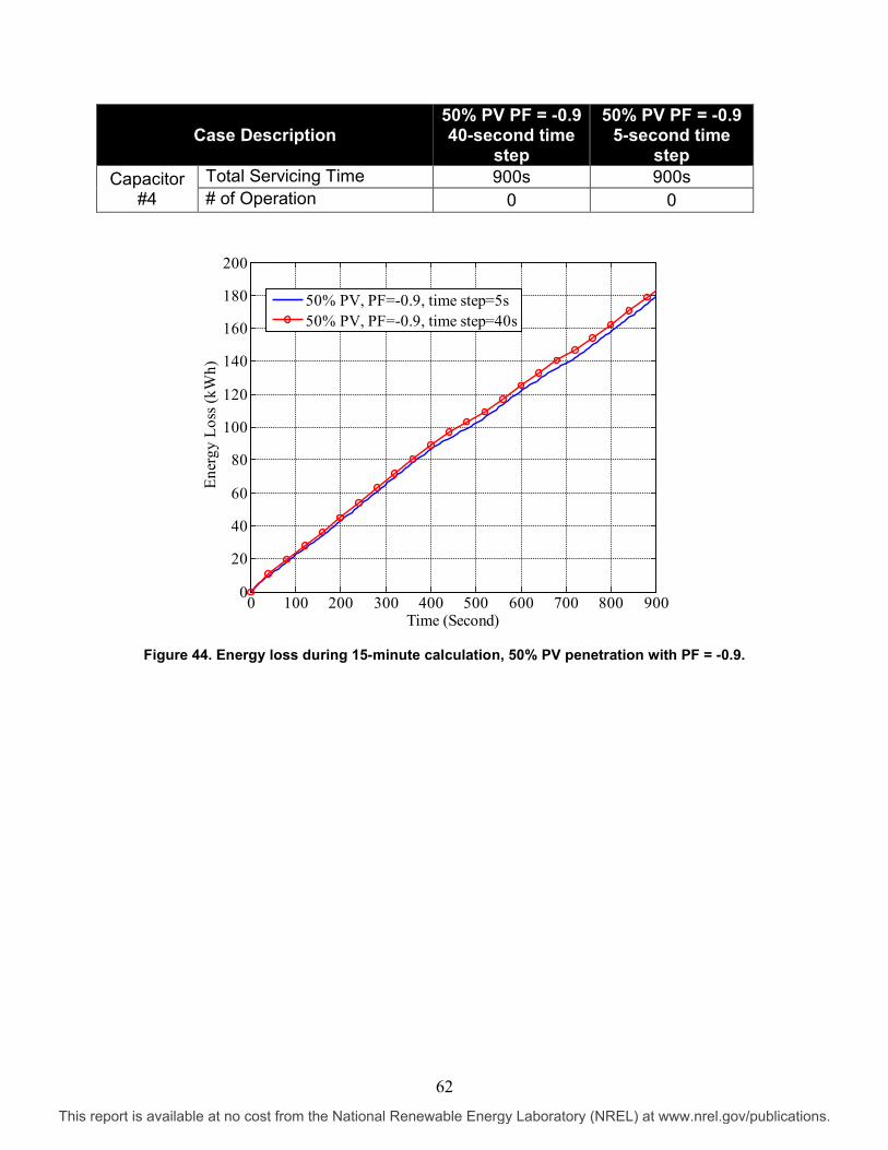
Case Description 50% PV PF = -0.9 40-second time

step

50% PV PF = -0.9 5-second time

step Capacitor

#4 Total Servicing Time 900s 900s # of Operation 0 0

Figure 44. Energy loss during 15-minute calculation, 50% PV penetration with PF = -0.9.

0 100 200 300 400 500 600 700 800 9000

20

40

60

80

100

120

140

160

180

200

Time (Second)

Ener

gy L

oss (

kWh)

50% PV, PF=-0.9, time step=5s50% PV, PF=-0.9, time step=40s

62


Comparison of 50% PV with PF = -0.95 at Power Factor Control Mode Case Table 12. Comparison of LTC, Voltage Regulators, and Capacitors Operations in 50% PV with PF =

0.95 Case

Case Description 50% PV PF = -0.95

40-second time step

50% PV PF = -0.95 5-second time step


Regulator2

Phase A

Max Tap Position 6 6

Min Tap Position 5 5

# of changes 1 1

Phase B



# of changes 5 3

Phase C



# of changes 2 5

Regulator3

Phase A



# of changes 1 2

Phase B



# of changes 8 9

Phase C



# of changes 4 5

Regulator4 Phase A



63


Case Description 50% PV PF = -0.95

40-second time step

50% PV PF = -0.95 5-second time step

# of changes 2 2

Phase B



# of changes 6 4

Phase C



# of changes 7 5 Capacitor

#1 Total Serving Time 900s 470s # of Operation 0 1

Capacitor #2

Total Serving Time 900s 900s # of Operation 0 0

Capacitor #4

Total Serving Time 900s 900s # of Operation 0 0

Figure 45. Energy loss during 15-minute calculation, 50% PV penetration with PF = -0.95.

0 100 200 300 400 500 600 700 800 9000

20

40

60

80

100

120

140

160

180

200

Time (Second)

Ener

gy L

oss (

kWh)

50% PV, PF=-0.95, time step=5s50% PV, PF=-0.95, time step=40s

64


Simulation Results for Inverters with Different Control Schemes In this section we present analysis results of OpenDSS models, the intent of which is to evaluate the effectiveness of PV inverter controls.

The objective is to determine and compare the applicability of the reactive power compensation methods for each of the following cases. The cases explore situations with single or multiple PV systems connected into the same part of a feeder, in close proximity to each other:

• 1 PV system (2 MW) in service (at the end of feeder): Cases with a PV reactive power control solution or no solution

• 2 PV systems (4 MW total) in service: Cases applying two different controls or same control on both units, but utilizing different settings

• 3 PV systems (5.5 MW total) in service: Cases with different controls or different settings.

The goal is to determine if the type of mitigation solution will vary according to the combination of the PV systems in service, as well as what type of controls provide the most effective solution for voltage regulation while minimizing adverse impact on the feeder operation. We present three base cases and two comparison cases.

Base Case 1: Different Inverter Controls for 50% (1 MW) and 100% (2 MW) of PV Generation The simulation studies in this section are for only one 2 MW PV system connected, with constant 50% and 100% solar irradiance levels applied. Only fixed loads are present, i.e., no variable loads are included in these simulations. The following inverter reactive power control schemes are simulated:

• PV with unity PF

• PV with inductive PF of -0.95 and -0.9

• PV with voltage droop control and droop coefficient of 3%, 5%, and 10% (Vref is 1.025 pu and deadband is 2%).

Simulation results for the above cases are shown below. The results are compared with the "No PV" scenario. The illustrations for each control scenario include the following:

• Voltage profile of the feeder as a function of the distance from the substation

• Voltage profile per phase for the final (steady-state) condition

• Voltage profile for different PV output and/or different inverter reactive power controls.

65


Figure 46. Studied system final state – Phase A voltage profile with different levels of PV

generation (fixed load, fixed 100% solar irradiance).

Figure 47. Studied system final state – Phase B voltage profile (fixed load, fixed 100% solar irradiance).

0 2 4 6 8 10 12 14 16 180.94

0.96

0.98

1

1.02

1.04

Distance from substation (km)

Vol

tage

(pu)

No PV50% PV, PF=1100% PV, PF=1

0 2 4 6 8 10 12 14 16 180.95

0.96

0.97

0.98

0.99

1

1.01

1.02

1.03

1.04

1.05


Vol

tage

(pu)


66


Figure 48. Studied system final state – Phase C voltage profile (fixed load, fixed 100% solar

irradiance).

Figure 49. Studied system final state – Phase A voltage profile with different power factor (fixed

load, fixed 50% solar irradiance).

0 2 4 6 8 10 12 14 16 18

1.02

1.025

1.03

1.035

1.04

1.045

1.05

1.055

1.06


Vol

tage

(pu)


0 2 4 6 8 10 12 14 16 180.94

0.96

0.98

1

1.02

1.04

1.06


Vol

tage

(pu)

50% PV, PF=150% PV, PF=-0.9550% PV, PF=-0.9

67


Figure 50. Studied system final state – Phase B voltage profile with different power factor (fixed


Figure 51. Studied system final state – Phase C voltage profile with different power factor (fixed


0 2 4 6 8 10 12 14 16 180.97

0.98

0.99

1

1.01

1.02

1.03

1.04

1.05

1.06


Vol

tage

(pu)

50% PV, PF=150% PV, PF=-0.9550% PV, PF=-0.9

0 2 4 6 8 10 12 14 16 18

1.02

1.025

1.03

1.035

1.04

1.045

1.05

1.055

1.06


Vol

tage

(pu)

50% PV, PF=150% PV, PF=-0.9550% PV, PF=-0.9

68


Figure 52. Studied system final state – Phase A voltage profile with different power factor (fixed


Figure 53. Studied system final state – Phase B voltage profile with different power factor (fixed


0 2 4 6 8 10 12 14 16 180.96

0.98

1

1.02

1.04

1.06

1.08


Vot

lage

(pu)

100% PV, PF=1100% PV, PF=-0.95100% PV, PF=-0.9

0 2 4 6 8 10 12 14 16 180.97

0.98

0.99

1

1.01

1.02

1.03

1.04

1.05

1.06


Vol

tage

(pu)

100% PV, PF=1100% PV, PF=-0.95100% PV, PF=-0.9

69


Figure 54. Studied system final state – Phase C voltage profile with different power factor (fixed


Figure 55. Studied system final state – Phase A voltage profile with different droop coefficient

(fixed load, fixed 50% solar irradiance; three different droop controls generate the same voltage profile).

0 2 4 6 8 10 12 14 16 181.02

1.025

1.03

1.035

1.04

1.045

1.05

1.055


Vol

tage

(pu)

100% PV, PF=1100% PV, PF=-0.95100% PV, PF=-0.9

0 2 4 6 8 10 12 14 16 180.95

0.96

0.97

0.98

0.99

1

1.01

1.02

1.03

1.04

1.05


Vol

tage

(pu)

50% PV, PF=150% PV, Droop Coef = 3%50% PV, Droop Coef = 5%50% PV, Droop Coef = 10%

70


Figure 56. Studied system final state – Phase B voltage profile with different droop coefficient


Figure 57. Studied system final state – Phase C voltage profile with different droop coefficient


0 2 4 6 8 10 12 14 16 180.95

0.96

0.97

0.98

0.99

1

1.01

1.02

1.03

1.04

1.05


Vol

tage

(pu)


0 2 4 6 8 10 12 14 16 18

1.02

1.025

1.03

1.035

1.04

1.045

1.05

1.055

1.06


Vol

tage

(pu)


71


Figure 58. Studied system final state – Phase A voltage profile with different droop coefficient


Figure 59. Studied system final state – Phase B voltage profile with different droop coefficient


0 2 4 6 8 10 12 14 16 18

0.96

0.98

1

1.02

1.04

1.06


Vol

tage

(pu)


0 2 4 6 8 10 12 14 16 180.97

0.98

0.99

1

1.01

1.02

1.03

1.04

1.05

1.06


Vol

tage

(pu)


72


Figure 60. Studied system final state – Phase C voltage profile with different droop coefficient


The study results showed that:

• Addition of the 50% PV generation (1 MW) toward the end of the feeder has improved the voltage profile of the feeder; therefore, reactive power compensation schemes are not necessary. It is more beneficial to operate the PV facility close to unity PF.

• The voltage violations on specific parts of the feeder and branches start to show up for full PV output (2 MW).

• Reactive power compensation has been able to effectively correct voltage profile (lower and maintain in the permissible range) on the first part of the feeder. However, it can adversely affect voltages on specific branches, further from the backbone.

• Voltage vs. distance plots are helpful in investigating the voltage issues for the entire feeder.

For the base study case, when there is only one centralized PV system on a feeder, the PF scheduling and voltage droop control schemes presented similar effects on the feeder voltages.

0 2 4 6 8 10 12 14 16 181.02

1.025

1.03

1.035

1.04

1.045

1.05

1.055


Vol

tage

(pu)


73


Base Case 2: Different Inverter Controls under Variable PV Profile and Variable Loads For this case, variable loads are included and all three PV systems are connected and a variable PV profile is applied. The simulation cases demonstrate the effect of the following controls:

• PV with unity PF

• PV with inductive PF of -0.95 or -0.9

• PV with droop control of 5% (reference voltage 1.025 pu, deadband 0.02 pu). The voltage profiles show the effect of PV output variations on voltages at the three PV sites by time for a 900-second (15-minute) PV profile.

Figure 61. Voltage at PV POIs when PV systems operate at unity PF.

1000 1100 1200 1300 1400 1500 1600 1700 1800 19000.98

1

1.02

1.04

1.06

1.08

1.1

Time (Second)

Vol

tage

(pu)

PV1, PF = 1PV2, PF = 1PV3, PF = 1

74


Figure 62. Voltage at PV POIs when PV systems operate at PF = -0.9.

Figure 63. Voltage at PV POIs when PV systems operate at PF = -0.95.

1000 1100 1200 1300 1400 1500 1600 1700 1800 1900

1.02

1.025

1.03

1.035

1.04

1.045

1.05

1.055

1.06

Time (second)

Vol

tage

(pu)

PV 1, PF = -0.9PV 2, PF = -0.9PV 3, PF = -0.9

1000 1100 1200 1300 1400 1500 1600 1700 1800 19001.015

1.02

1.025

1.03

1.035

1.04

1.045

1.05

1.055

1.06

Time (Second)

Vol

tage

(pu)

PV 1, PF = -0.95PV 2, PF = -0.95PV 3, PF = -0.95

75


Figure 64. Reactive power of each PV system for operation at 0.95 leading power factor

(absorbing).

Figure 65. Voltage at PV POIs when PV systems operate with 5% droop control mode.

1000 1200 1400 1600 1800 20000

100

200

300

400

500

600

700

Time (Second)

Rea

ctiv

e Po

wer

(kV

Ar)

PV 1, PF=-0.95PV 2, PF=-0.95PV 3, PF=-0.95

1000 1100 1200 1300 1400 1500 1600 1700 1800 19001.01

1.015

1.02

1.025

1.03

1.035

1.04

1.045

Time (Second)

Vol

tage

(pu)

PV 1, Droop Coef = 5%PV 2, Droop Coef = 5%PV 3, Droop Coef = 5%

76


Figure 66. Reactive power of each PV system for 5% droop control (absorbing Q).

The study results showed that:

• Using fixed or scheduling PF, low PFs (as low as 0.9 or lower) will be required to avoid voltage violations.

• With multiple PV systems on a feeder, voltage profile adjustment can be better achieved with voltage droop control than with PF control. With this scheme, the reactive power compensation level is directly determined from the range of voltage deviations, and extensive up front studies are not required to determine PF scheduling levels or pre-specifications of reactive power set points.

1000 1200 1400 1600 1800 20000

200

400

600

800

1000

1200

Time (Second)

Rea

ctiv

e Po

wer

(kV

Ar)

PV 1, Droop Coef=5%PV 2, Droop Coef=5%PV 3, Droop Coef=5%

77


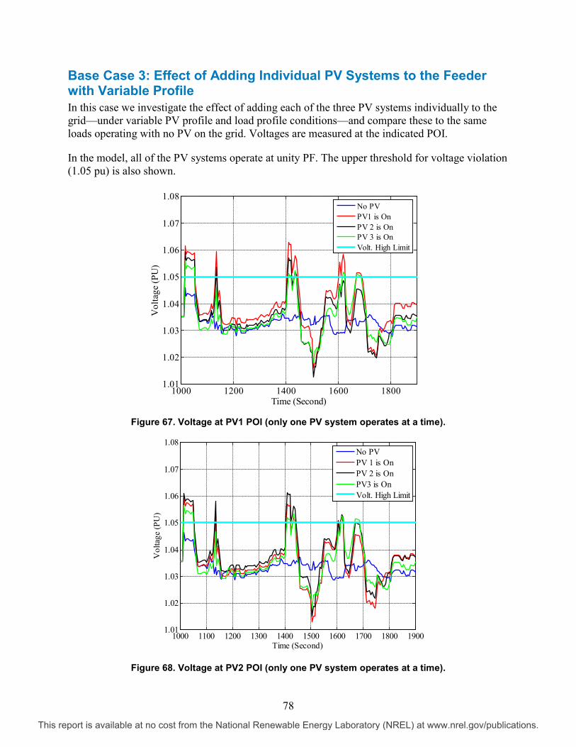
Base Case 3: Effect of Adding Individual PV Systems to the Feeder with Variable Profile In this case we investigate the effect of adding each of the three PV systems individually to the grid—under variable PV profile and load profile conditions—and compare these to the same loads operating with no PV on the grid. Voltages are measured at the indicated POI.

In the model, all of the PV systems operate at unity PF. The upper threshold for voltage violation (1.05 pu) is also shown.

Figure 67. Voltage at PV1 POI (only one PV system operates at a time).


1000 1200 1400 1600 18001.01

1.02

1.03

1.04

1.05

1.06

1.07

1.08

Time (Second)

Vol

tage

(PU

)

No PVPV1 is OnPV 2 is OnPV 3 is OnVolt. High Limit

1000 1100 1200 1300 1400 1500 1600 1700 1800 19001.01

1.02

1.03

1.04

1.05

1.06

1.07

1.08

Time (Second)

Vol

tage

(PU

)

No PVPV 1 is OnPV 2 is OnPV3 is OnVolt. High Limit

78



From the above figures, it can be seen that each individual PV system working at full power generation can result in the voltage exceeding the high limit.

1000 1100 1200 1300 1400 1500 1600 1700 1800 19001

1.01

1.02

1.03

1.04

1.05

1.06

Time (Second)

Vol

tage

(PU

)

No PVPV 1 is OnPV 2 is OnPV 3 is OnVolt. High Limit

79


Comparison Case 1: Multiple PV Systems with Different Power Factor Settings In this section we investigate the effects on feeder voltages of using PV systems with different PFs. The simulations are based on variable load and variable solar irradiance profiles. PV1 (2 MW) is set at a PF of -0.9, PV2 (2 MW) at a PF of -0.9, and PV3 (1.5 MW) at a PF of -0.95. The voltages at the POI of the PV systems are shown and compared with the case of PV systems using unity PF. Voltages at two variable load locations (loads 3 and 6) are also shown for similar conditions (unity vs. non-unity PF for PV systems). Loads 3 and 6 are on the branch of the feeder where there is no PV connected.

Figure 70. Comparison of voltages at PV POIs when PV systems use unity power factor vs. non-

unity power factors.

1000 1100 1200 1300 1400 1500 1600 1700 1800 19000.98

1

1.02

1.04

1.06

1.08

1.1

Time (Second)

Vol

tage

(pu)

PV 1, PF = 1PV 2, PF = 1PV 3, PF = 1PV 1, PF = -0.9PV 2, PF = -0.9PV 3, PF = -0.95

80


Figure 71. Comparison of voltages at load 3 and 6 when PVs use unity power factor vs. non-unity

power factors.

The reactive power of the PV systems and a comparison of the losses are shown in the following figures. Compared to unity PF operation, the additional system losses due to reactive power absorption by PV systems with non-unity PFs are negligible.

Figure 72. Reactive power of the PV systems with non-unity power factors.

1000 1100 1200 1300 1400 1500 1600 1700 1800 19000.98

1

1.02

1.04

1.06

1.08

1.1

Time (Second)

Vol

tage

(pu)

Load 3, PVs in PF=1Load 6, PVs in PF=1Load 3, PVs in different PFLoad 6, PVs in different PF

1000 1200 1400 1600 1800 2000 22000

200

400

600

800

1000

Time (Second)

Rea

ctiv

e Po

wer

(kV

Ar)

PV 1, PF=-0.9PV 2, PF=-0.9PV 3, PF=-0.95

81


Figure 73. Comparison of system kWh losses when PV inverters use unity power factor vs. non-

unity power factors.

It can be seen from the results that utilizing non-unity PF has been an effective scheme for lowering the voltage variations. Although system losses have slightly increased under non-unity PF condition, the changes are insignificant.

0 100 200 300 400 500 600 700 800 9000

50

100

150

Time (Second)

Ener

gy L

oss (

kWh)

100% PV, PF=1100% PV, different PF

82


Comparison Case 2: PV Systems with Different Control Strategies This case compares the effect of applying different control methods to PV systems. The legacy PV systems are expected to only have the control option of adjusting PF, while newer PV inverters (equipped with smart inverter features) may be able to provide various control options. As an example of mixing control schemes, PV1 is assumed to work with 4% droop control mode (reference voltage = 1.025 pu, deadband = 0.02 pu), PV2 works at 0.9 PF (absorbing Q), and PV3 works at fixed absorbing reactive power with a setting of 25% of the rated 1.5 MW active power, i.e., 375 kVAr. The results are compared with a case in which PV1 works at PF = -0.9, PV2 works at PF = -0.9, and PV3 works at PF = -0.95. Voltages at various PV POIs and selected load locations are shown in the figure for comparison. Variable loads and a variable PV profile are included.

Figure 74. Comparison of voltages at PV POIs when PV systems are operating with different

control strategies.

1000 1100 1200 1300 1400 1500 1600 1700 1800 19001.02

1.025

1.03

1.035

1.04

1.045

1.05

1.055

1.06

Time (Second)

Vol

tage

(pu)

PV1, PF = -0.9PV2, PF = -0.9PV3, PF = -0.95PV1, Drop Coef = 4%PV 2, PF = -0.9PV3, Const Q = 25%*Rated P

83


Figure 75. Comparison of voltages at loads 3 and 6 when PV systems use different control

strategies.

Figure 76. Reactive power of the PV systems for various control strategies.

1000 1100 1200 1300 1400 1500 1600 1700 1800 19001.02

1.025

1.03

1.035

1.04

1.045

1.05

1.055

1.06

1.065

Time (Second)

Vol

tage

(pu)

Load 3, PVs with fixed PFLoad 6, PVs with fixed PFLoad 3, PVs with different controlLoad 6, PVs with different control

600 800 1000 1200 1400 1600 18000

200

400

600

800

1000

1200

Time (Second)

Rea

ctiv

e Po

wer

(kV

Ar)

PV1, PF=-0.9PV2, PF=-0.9PV3, PF=-0.95PV1, Droop Coef=4%PV2, PF=-0.9PV3, Q=25% rated P

84


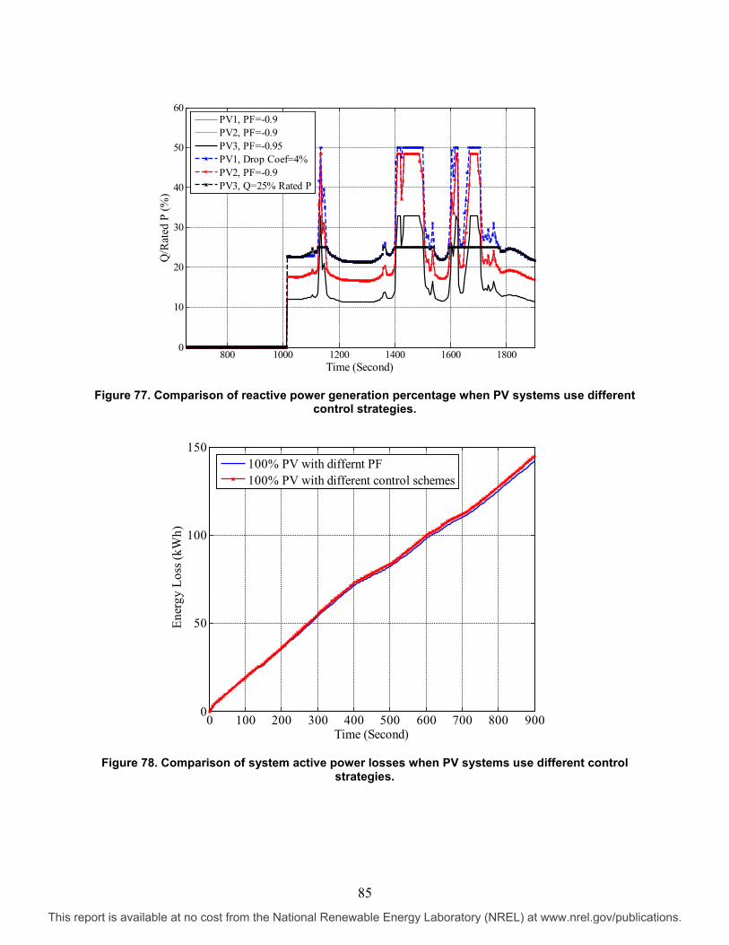
Figure 77. Comparison of reactive power generation percentage when PV systems use different

control strategies.

Figure 78. Comparison of system active power losses when PV systems use different control

strategies.

800 1000 1200 1400 1600 18000

10

20

30

40

50

60

Time (Second)

Q/R

ated

P (%

)

PV1, PF=-0.9PV2, PF=-0.9PV3, PF=-0.95PV1, Drop Coef=4%PV2, PF=-0.9PV3, Q=25% Rated P

0 100 200 300 400 500 600 700 800 9000

50

100

150

Time (Second)

Ener

gy L

oss (

kWh)

100% PV with differnt PF100% PV with different control schemes

85


The simulation results show that droop control has been effective in lowering the voltage profile and maintaining it in the permissible range. In addition, unnecessary capacitor switching has been prevented.

Summary and Conclusions The main objective of the reported studies was to investigate the modeling of various reactive power compensation schemes as part of large PV systems, and the applicability of the schemes for time-series analysis. The modeling was performed in the OpenDSS software tool and utilized time-series analysis for investigating PV impact on a reduced version of the IEEE 8500 node benchmark feeder.

In order to determine the effectiveness of the reactive power controls in mitigating voltage violations caused by high penetration of MW-size PV systems, several case studies were analyzed. Multiple study scenarios were investigated including:

• PV systems with similar reactive power control schemes, such as fixed PF or voltage droop controls applied to all PV facilities, and

• PV systems with varying reactive power control schemes on a feeder. The study results showed that:

• The commonly used reactive power control schemes as part of commercial PV systems can be modeled and included in time-series analysis for PV impact studies using open-source software tools such as OpenDSS.

• It is beneficial to develop and suggest standard control methods and modeling approaches to ensure model implementations and studies will not be different from one software platform to another. Some common schemes were introduced and modeled in this report.

• It is essential to investigate voltage profiles for the entire feeder, as well as for branches and laterals. Due to the interactions with voltage regulators, although reactive power compensation can mitigate voltage violations on part of a feeder, there may be cases where the voltages are adversely affected in other areas. To reduce reactive power demand from the system at low PV production levels—where a PV system can potentially operate at unity PF with no voltage violations—PF scheduling is a preferred control scheme, compared to using fixed PF set points.

• With multiple PV systems on a feeder, voltage droop control can provide tighter voltage profile adjustment than can PF control. With this scheme, the reactive power compensation level is directly determined from the range of voltage deviations, and does not need extensive upfront studies to determine PF scheduling levels or pre-specifications of reactive power set points.

• When dealing with a mix of legacy PV systems that may only have the PF adjustment scheme and new PV systems with multiple control schemes, voltage droop control can still be a safe control selection to avoid possible interactions among units, while optimizing the voltage profile and reactive power demand of the feeder.

86


References [1] OpenDSS software and application guides, available online: http://sourceforge.net/projects/electricdss/files.

[2] D. Paradis, F. Katiraei, B. Mather, “Comparative Analysis of Time-Series Studies and Transient Simulations for Impact Assessment of PV Integration on Reduced IEEE 8500 Node Feeder,” in Proc. IEEE PES General Meeting, Vancouver, BC, July 2013.

[3] B. Mather, “Quasi-static time-series test feeder for distributed PV integration analysis,” in Proc. IEEE PES General Meeting, San Diego, CA, 2011.

[4] R. F. Arritt, R.C. Dugan, “The IEEE 8500-Node Test Feeder,” in Proc. IEEE PES Transmission and Distribution Conference and Exposition, 2010.

87


http://sourceforge.net/projects/electricdss/files

Appendix A: Reduced IEEE 8500 Node Feeder Representation

The reduced IEEE 8500 feeder used in the time-series studies is shown in the figure above [2]. The figure shows the location of the loads and aggregated feeder sections to reduce the size of the feeder as required for the studies. The corresponding node numbers and location of the major voltage control devices are also shown in the figure.

The sum of the loads and capacitors between the source of the feeder and the first branching out at node #174, for example, varies between the three phases, as shown in the table below.

Table 13. Total Loads between Feeder Source and First Branch at Node #174

Phase Total Real Power Loads (kW)

Total Reactive Power Loads (KVAr)

A 302.9 -519.3 B 192.8 -548.7 C 473.8 -473.1

Node#482

Nodes #1, 2 & 8

300 kVAR300 kVAR300 kVAR

Node#9

Nodes #11, 13, 15, 78, 81, 120, 133,

136, 155, 163, 166, 170 & 174


Node#170

Node#174

Voltage Controlled

Voltage Controlled

Regulator #4


Node#255

Manual Control

End of Branch

Regulator #2


Node#453

Voltage Controlled

Regulator #3

Node#468

End of Branch

Node#481

End of Branch

Node#472

Node#476

Node#672

End of Branch

End of Branch End of

Branch

Not all node numbers are used Nominal, 115kV L-L RMS

Actual, 1.05 p.u.

13.09[kV] : 115[kV]

r

Nodes #177, 178, 182, 185, 186,

197, 198, 199, 203, 206, 207, 209, 215, 222, 226, 229 &

230

Nodes #231, 233, 234, 235, 236,

238, 240, 243, 247, 248, 249, 252 &

254

Nodes #259, 260, 262, 264, 269,

271, 277, 284, 288, 291, 295, 296, 298, 299, 300, 301 &

302

Nodes #308, 309, 310, 314,

315, 317, 320, 323, 326, 328, 329, 330, 338, 346, 349, 353,

360 & 364

Nodes #366, 397, 407, 423, 445 & 451

Nodes #456 & 458

Nodes #458, 459, 463, 465 & 467

Nodes #489, 499, 502,

506, 512, 515, 519, 524, 535, 540 &

542

Node#546

Nodes #556, 560, 566, 573, 580, 587,

594, 603

Node#606

Nodes #648, 654, 662 & 670

Node#689 Nodes #679 &

684

Node#719 Nodes #693,

701, 714 & 718

Node#642 Nodes #617, 626,

631 & 635

Figure 79. General layout of simplified 8500 node feeder system.

88


The load through the branch from #174 to #302 is also not evenly distributed.

Table 14. Total Loads between Node #174 and #302

Phase Total Real Power Loads (kW)

Total Reactive Power Loads (kvar)

A 801.9 -87.3 B 919.9 -55.7 C 1207.2 22.6

This, of course, also means that the load through the other side of the feeder (#174 down) will also be unevenly distributed. Most importantly, the total power from phase C going down the feeder in that direction will be substantially lower than that for the other two phases, which will affect the operation of the regulators (which are operated individually per phase) and explains the different tap settings between the three phases.

Loads Loads are represented with fixed dynamic load models, each representing a single phase load at any given node. The real and reactive power flows into the loads were determined from the OpenDSS simulation. Loads were set up with parameters dP/dV = 1 and dQ/dV = 2.

Table 15. Load Parameters

Parameter Value dP/dV 1 dQ/dV 2

Lines The line lengths were preserved (several line sections were grouped into one if no loads or nodes were present between them). To simplify the modeling, the lines were converted to a single line type. Line impedances are represented by their positive and zero sequence resistance, impedance, and shunt capacitance.

89


Table 16. Transmission Line Parameters

Line Type 397 ACSR 4F/S C Neutral 1/0 ACSR 2F/S I Spacing HORIZONTAL 3P 52 Parameters Rated Frequency 60 Hz Zero-sequence Capacitive

reactance 2.922 MΩ*mi

Zero-sequence Inductive Reactance

2.127 Ω/mi

Zero-sequence Resistive Reactance

0.9512 Ω/mi

Positive-sequence Capacitive reactance

6.901 MΩ*mi

Positive-sequence Inductive Reactance

0.6185 Ω/mi

Positive-sequence Resistive Reactance

0.2537 Ω/mi

The per-unitizing feeder voltage base is set to 12.47 kV rms, line-to-line (L-L).

Capacitor Controls The capacitor controls were set based on the available OpenDSS model information. Capacitors #1, #2, and #4 are controlled based on feeder voltages, while capacitor #3 is manually controlled (and fixed for these simulations). The capacitors are controlled under three different conditions:

• “Normal” conditions, where the voltage remains within a reasonable margin of expected,

• Slow response, where voltages are outside normal range, but within extreme range, and

• “Extreme” conditions, where the voltage fluctuations are more significant and requires the capacitors to operate.

If the voltage fluctuates outside of the “extreme” range, the capacitor operates faster to prevent problems. The voltage limits in OpenDSS of 0.9785–1.075 pu are used as the limits of the “extreme” range and the normal range was defined as 1.0–1.05 pu. If the voltage fluctuates outside of the “normal” range, but within the “extreme” range, the capacitor operation time is set to 60 seconds. If the voltage fluctuates outside the “extreme” range, the operation time is reduced to 5 seconds. Once a capacitor operates, it will not operate again for 300 seconds or 5 minutes.

90


Table 17. Capacitor Control Parameters

Parameter Value Extreme minimum voltage 0.9785 pu

Extreme maximum voltage 1.075 pu

Normal minimum voltage 1.0 pu

Normal maximum voltage 1.05 pu

Extreme operation time 5 seconds

Normal operation time 60 seconds

Minimum time between operations 300 seconds

LTC and Regulator Controls The LTC at the source of the feeder has a single tap control for all three phases. The primary side of the transformer is connected to the source at 115 kV rms, L-L, and the secondary side of the transformer is rated for 13.0935 kV rms, L-L, or 1.05 pu. The tap value of the transformer can vary from 0.9 to 1.1, and the target range is 1.0458–1.0625 pu, with a tap step change of 0.00625. The LTC can operate every 30 seconds.

Voltage regulators #2, #3, and #4 are controlled individually on each phase. Both the primary and secondary windings are rated for 12.47 kV rms, L-L. The tap value of the regulator can vary from 0.9–1.1 pu, and the target range is from 1.0333–1.05 pu, with a tap step change of 0.00625. The regulators can operate every 45 seconds.

Table 18. LTC and Voltage Regulators Control Parameters

Parameter LTC Regulators Minimum voltage 1.0458 pu 1.0333 pu

Maximum voltage

1.0625 pu 1.05 pu

Number of taps 32 32

Minimum tap 0.9 0.9

Maximum tap 1.1 1.1

Operation delay 30 s 45 s

Control 3-phase 1-phase

Reversible No No

A load equivalent to an adjacent feeder was also added to the system directly at the secondary tap of the LTC to increase loading on the system (this was not in the published OpenDSS model). The load is distributed evenly between all three phases and is approximately the same size (both in real and reactive power) as the feeder. Each phase represents a load of 3896.3 kW and 279.7 kVAr.

91


PV Systems and Generation Profile Three PV systems were added to the feeder on the far side of regulator #3:

• 2000 kW at node #546

• 2000 kW at node #642

• 1500 kW at node #719.

Figure 80. PV generation profile used for simulations (x-axis is time in min).

These values were chosen so that, if all PV systems are operating at full power, the real power flow direction will be reversed across regulator #3 but remain positive across regulator #2. This system was then simulated with all three PV systems at full power to verify correct operation of the capacitors, LTC, and regulators. Once this was done, the system was simulated using a 15-minute power generation profile—as shown in Figure 80—to study the response of the controls to the power changes from the PV systems.

Variable Loads Selected large size loads were made variable. The variable loads were added to the feeder to investigate interaction of load and generation. The rest of the fixed loads in the model were considered as dynamic loads with voltage dependency (dP/dV = 1 and dQ/dV = 2). P & Q of the loads are calculated as:

𝑃 = 𝑃0 𝑉𝑉0𝑑𝑃/𝑑𝑉

,𝑄 = 𝑄0 𝑉𝑉0𝑑𝑄/𝑑𝑉

where:

𝑃0 = rated real power per phase

𝑄0 = rated reactive power per phase

𝑉0 = rated voltage

92


Using these equations, the values of R and L can then be calculated as:

𝑅 = 𝑉2

𝑃0𝑉𝑉0

𝐿 = 𝑉2

𝜔𝑄0 𝑉𝑉02

Large loads distributed throughout the feeder have been set up to vary over time. Their approximate positions in the feeder are shown in Figure 81.

Figure 81. Location of the variable loads in the feeder.

The variable loads will be simulated using six different profiles for both the real and reactive power. The loads selected and the associated profiles are detailed in the table below.

Table 19. Variable Loads Used During Simulations and Associated Profiles

Node # Rated power (kVA) Profile # Phase A Phase B Phase C 81 121.2 178.0 134.8 1 236 371.6 2 296 139.1 3 302 267.0 3 338 225.4 296.6 92.2 4 423 53.0 434.5 65.1 5 594 104.4 364.6 6 606 36.1 259.1 6

The load profiles used for both real and reactive power (scaled to pu) are shown in the following figure.

93


Figure 82. Profiles used for variable loads (in per unitized of rated value).

94


Appendix B: System Parameters A. Source Information

Source Amplitude

Source Impedance

Pos. Sequence Zero Sequence

115 kV (L-L rms) 21.81099, 88.0908 deg

65.43296, 88.0908 deg

B. List of Loads

Node Number

Phase A Phase B Phase C

P (kW) Q (kVAr) P (kW) Q

(kVAr) P (kW) Q (kVAr)

Source

1 Adjacent Feeder 3896.3 279.7 3896.3 279.7 3896.3 279.7 2 Load

4.1 1.1

8 Load 1.8 0.5 9 Capacitor 1 -300 -300 -300

11 Load

259 69.7 13 Load 39.7 10.6

15 Load

6.2 1.6 78 Load 14.4 3.8

81 Load 117.1 31.3 172 45.7 130.3 34.7 120 Load

43.3 11.5

133 Load 18.1 4.8 136 Load 55.9 14.8 5.9 1.6

155 Load 14.4 3.8 163 Load 9 2.4

4.1 1.1 166 Load

26.8 7.2

170 Capacitor 2 -300 -300 -300 174 Load 32.5 8.7 14.9 4

FORK

BRANCH OUT OF 174

177 Load 5.4 1.4

15.5 4.1 178 Load

37.1 9.9

182 Load 9 2.4

16.5 4.5 185 Load

33.6 8.8

186 Load 55.9 14.8 35.6 9.3 197 Load 37.8 10

206 5.6

198 Load

15.5 4.1 199 Load

72.1 19.2

95


Node Number




203 Load 14.4 3.8 9.9 2.6 10.3 2.8 206 Load 5.4 1.4

419.7 112.6

207 Load

6.2 1.7 209 Load 9 2.4 46.4 12.3

215 Load

5.9 1.6 20.6 5.6 222 Load 71.2 19 45.9 12.1 46.6 12.4 226 Load 12.6 3.3

229 Load 9 2.4 9.9 2.6 230 Load 18.1 4.8

231 233 Load

76.2 19.8

234 Load 5.4 1.4

6.2 1.6 235 Load

6.2 1.6

236 Load

359.1 95.6 238 Load

6.2 1.6

240 Load

4.1 1.1 243 Load 134.3 35.9

247 Load 14.4 3.8

29.9 8 248 Load 5.4 1.4

6.2 1.6

249 Load 3.6 1 5.9 1.6 252 Load 14.4 3.8

12.4 3.3

254 Load 28.8 7.2 226.6 60.5 255 Capacitor 3 -300 -300 -300

259 Load 18 4.8

31 8.3 260 Load 18 4.8

262 Load 27 7.1 264 Load 18 4.8 14.9 4

269 Load 14.4 3.8 11.9 3.1 271 Load 71.2 19 3.9 1.1 4.1 1.1

277 Load 9 2.4 19.8 5.2 72.3 19.3 284 Load 5.4 1.4

10.3 2.8

288 Load 9 2.4

15.5 4.1 291 Load

15.8 4.2 28.9 7.7

295 Load 9 2.4 9.9 2.6 296 Load 134.4 35.8

298 Load 9 2.4 5.9 1.6 299 Load

6.2 1.6

300 Load

11.8 3.2

96


Node Number




301 Load 5.4 1.4 302 Load

258 68.9

END OF BRANCH

BRANCH OUT OF 174

308 Load 18.1 4.8

25.8 6.9 309 Load

12.4 3.3

310 Load 13.5 3.6 314 Load

4.1 1.1

315 Load

26.8 7.1 317 Load 13.5 3.6

320 Load

28.8 7.7 323 Load

43.3 11.6

326 Load

24.7 6.6 10.3 2.8 328 Load

51.7 13.7

329 Load

40.6 10.8 330 Load 30.9 8.2 30 7.9 37.9 10

338 Load 218 57.3 286.8 75.6 89.2 23.3 346 Load 36.1 9.6 5.9 1.6

349 Load 27 7.2 353 Load 18 4.8

10.3 2.8 360 Load 106.5 28.3

8.2 2.2

364 Load 19.3 5.2 24.8 6.6 366 Load

77.6 20.6

397 Load 5.4 1.4 24.7 6.6 20.6 5.5 407 Load 43.2 11.5

20.7 5.5

423 Load 50.4 13.2 419.5 113.1 62.9 16.6 445 Load 3.6 1 3.9 1 14.4 3.9 451 Load 51.3 13.6

453 Capacitor 4 -400 -400 -400 456 Load 36.9 9.8 5.9 1.6

458 Load

9.9 2.6 459 Load 9 2.4

463 Load 13.5 3.6

15.5 4.1 465 Load 9 2.4

20.7 5.5

467 Load 13.5 3.6 468 Load 14.4 3.8

FORK

BRANCH OUT OF 468

97


Node Number




481 Load

20.6 5.5

FORK

BRANCH OUT OF 482 489 Load 14.4 3.8

16.5 4.5

499 Load 18.9 5

28.9 7.7 502 Load 12.6 3.3

506 Load 14.4 3.8 14.9 4 6.2 1.6 512 Load 9 2.4 9.9 2.6 10.3 2.7 515 Load 165.7 44.1

519 Load 41.5 11 51.6 13.8 57.1 15.2 524 Load 18.1 4.8 29.7 7.9 33.2 8.8 535 Load 88.3 23.4

14.4 3.8

540 Load 19.8 5.2

6.2 1.6 542 Load 9 2.4

20.6 5.5

546 Load 18 4.8

47.8 12.8

END OF BRANCH

BRANCH OUT OF 482 556 Load 159.7 42.7 35.6 9.4

560 Load 36.9 9.8 9.9 2.6 566 Load 9 2.4 9.9 2.6 143.8 38.2

573 Load 28.8 7.6 54.5 14.5 580 Load

41.5 11 61.9 16.5

587 Load 27 7.2 29.8 8 594 Load 100.9 26.9 352.1 94.5 603 Load 9 2.4

26.8 7.2

606 Load 36.1 9.2

250.6 65.8

END OF BRANCH

BRANCH OUT OF 468 472 Load 3.6 1

476 Load

10.3 2.8

FORK

BRANCH OUT OF 476 648 Load

9.9 2.6 130 33.9 654 Load 109.2 29.2 20.8 5.6 16.5 4.34 662 Load 269.6 71.9 9.9 2.6 20.6 5.6 670 Load 45.9 12.2 9.9 2.6 26.9 7.2 672 Load 9 2.4

FORK

98


Node Number




BRANCH OUT OF 672

679 Load 9 2.4 19.8 5.2 20.6 5.5 684 Load 3.6 1 263 70.2 93.2 24.9 689 Load 127.1 33.8 23.6 6.3

END OF BRANCH

BRANCH OUT OF 672

693 Load 9 2.4 24.8 6.6 701 Load 37.8 10 49.3 13.1 6.2 1.7

714 Load

59.2 15.7 4.1 1.1 718 Load

51.4 13.7 152.2 40.5

719 Load 161.7 43

END OF BRANCH

BRANCH OUT OF 476 617 Load 14.4 3.8

105.8 27.8

626 Load 70.2 18.7 9.9 2.6 20.8 5.5 631 Load 9 2.4 9.9 2.6 16.5 4.4 635 Load 14.4 3.8

20.6 5.5

642 Load 75.6 20.1 477.2 126.9

END OF FEEDER

C. List of Lines

From Bus

To Bus Length (ft)

1 2 82.85

2 8 1535.92

8 9 180.81

9 11 255.79

11 13 465.9

13 15 375.2

15 78 1033.66

78 81 523.35

81 120 1853.9

120 133 135.07

133 136 480.62

99


From Bus

To Bus Length (ft)

136 155 366.01

155 163 878.92

163 166 136.35

166 170 132.52

170 174 618.4

FORK

BRANCH OUT OF 174

174 177 968.51

177 178 239.48

178 182 849.22

182 185 437.43

185 186 246.02

186 197 1347.03

197 198 131.23

198 199 298.41

199 203 526.05

203 206 697.17

206 207 236.89

207 209 595.48

209 215 1654.18

215 222 1426.55

222 226 450.66

226 229 841.96

229 230 314.21

230 231 298.94

231 233 209.17

233 234 258.81

234 235 530.55

235 236 300.21

100


From Bus

To Bus Length (ft)

236 238 366.07

238 240 294.31

240 243 52.39

243 247 1086.77

247 248 409.99

248 249 329.89

249 252 1090.26

252 254 246.65

254 255 232.91

255 259 718.45

259 260 141.56

260 262 416.13

262 264 499.24

264 269 644.9

269 271 379.2

271 277 1110.08

277 284 669.12

284 288 618.26

288 291 776.89

291 295 741.97

295 296 167.15

296 298 399.34

298 299 151.32

299 300 186.24

300 301 118.31

301 302 112.1

END OF BRANCH

BRANCH OUT OF 174

174 308 748.41

101


From Bus

To Bus Length (ft)

308 309 165.95

309 310 220.32

310 314 708.34

314 315 125.18

315 317 1040.76

317 320 938.77

320 323 249.17

323 326 806.73

326 328 181.83

328 329 131.18

329 330 567.35

330 338 789.66

338 346 1004.55

346 349 379.51

349 353 572.22

353 360 1058.29

360 364 811.89

364 366 340.57

366 397 1807.32

397 407 2666.71

407 423 2246.94

423 445 1178.47

445 451 370.65

451 453 331.43

453 456 639.35

456 458 728.4

458 459 161.14

459 463 297.12

463 465 507.15

102


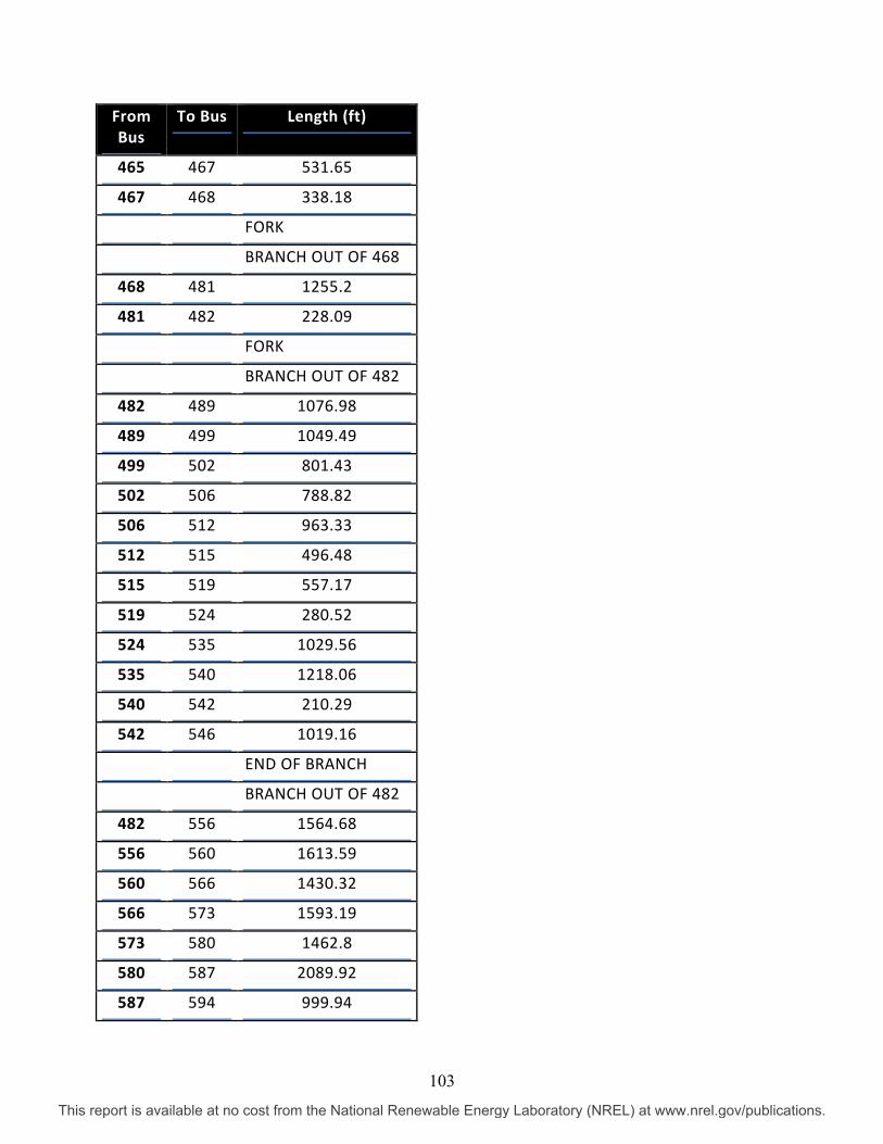
From Bus

To Bus Length (ft)

465 467 531.65

467 468 338.18

FORK

BRANCH OUT OF 468

468 481 1255.2

481 482 228.09

FORK

BRANCH OUT OF 482

482 489 1076.98

489 499 1049.49

499 502 801.43

502 506 788.82

506 512 963.33

512 515 496.48

515 519 557.17

519 524 280.52

524 535 1029.56

535 540 1218.06

540 542 210.29

542 546 1019.16

END OF BRANCH

BRANCH OUT OF 482

482 556 1564.68

556 560 1613.59

560 566 1430.32

566 573 1593.19

573 580 1462.8

580 587 2089.92

587 594 999.94

103


From Bus

To Bus Length (ft)

594 603 1258.39

603 606 295.36

END OF BRANCH

BRANCH OUT OF 468

468 472 287.97

472 476 1469.96

FORK

BRANCH OUT OF 476

476 648 1209.88

648 654 815.93

654 662 2485.2

662 670 1376.32

670 672 740.1

FORK

BRANCH OUT OF 672

672 679 1758.78

679 684 1522.39

684 689 1698.95

END OF BRANCH

BRANCH OUT OF 672

672 693 685.02

693 701 3322.56

701 714 3192.74

714 718 767.43

718 719 144.94

END OF BRANCH

BRANCH OUT OF 476

476 617 1469.96

617 626 1209.27

104


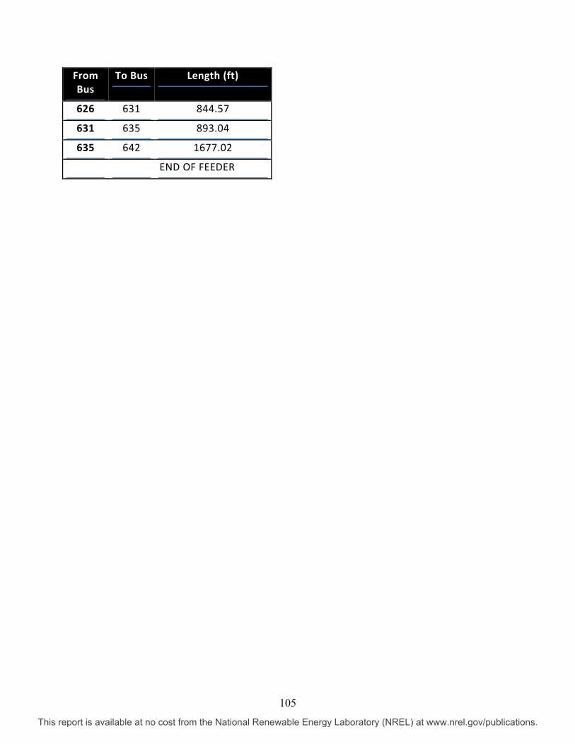
From Bus

To Bus Length (ft)

626 631 844.57

631 635 893.04

635 642 1677.02

END OF FEEDER

105


4 Methods for Performing High Penetration PV Studies

106


Abstract A methodology for performing high penetration PV studies is presented, along with an example of using the methodology. The methodology includes concepts from current available literature, several utilities, IEEE standards, and U.S. Department of Energy (DOE) reports. Detailed study criteria are presented and form the foundation for the methodology. The steps of a start-to-finish procedure are presented.

107


Table of Contents Abstract .................................................................................................................................................... 107 List of Figures ......................................................................................................................................... 108 List of Tables ........................................................................................................................................... 108 Introduction ............................................................................................................................................. 109

Background ........................................................................................................................................ 110 Areas of Concern ................................................................................................................................ 110

Criteria for Evaluation ............................................................................................................................. 112 Requirements for Study ......................................................................................................................... 115 Methods for Conducting High Penetration PV Studies ....................................................................... 116

Generation Time-Series Analysis—With and Without New PV ....................................................... 117 Generation Impact Analysis ............................................................................................................... 119 Generation Fault Analysis .................................................................................................................. 121 Mitigation ........................................................................................................................................... 122 High Penetration PV Study Outline and Steps ................................................................................... 123 Conclusions ........................................................................................................................................ 126

Overview of Fontana Area High Penetration Circuit Analysis ........................................................... 127 Summary ............................................................................................................................................ 127 Analysis Procedure ............................................................................................................................. 127

Appendix A: Typical PV Database Needs ............................................................................................. 139 Appendix B: Generation Impact Results Summary Form ................................................................... 141 Definitions ................................................................................................................................................ 143

List of Figures Figure 83. Customer voltage change vs. PV power factor at Fontana 3 MW PV .............................. 123 Figure 84. Fontana area circuit built within DEW. ............................................................................... 128 Figure 85. DEW's DER Assessment dialog. ......................................................................................... 131 Figure 86. Peak day native load. ............................................................................................................ 131 Figure 87. Minimum day native load. .................................................................................................... 132 Figure 88. On to off peak native load. ................................................................................................... 132 Figure 89. Customer voltage at POI vs. PV power factor. ................................................................... 136 Figure 90. Reverse flow visualization of Fontana. ............................................................................... 137

List of Tables Table 20. Criteria for Evaluating PV Generation Impacts ................................................................... 113 Table 21. Example Customer Voltage Change (in V on 120 V service) vs. PV Power Factor ......... 122 Table 22. Fontana Circuit Capacitor Settings ...................................................................................... 129 Table 23. Measurement Scan Rates ...................................................................................................... 129 Table 24. Approximated 2011 Capacitor Operation Base upon SCADA Measurements ................. 130 Table 25. Time-Series Analysis Customer Voltage Summary ............................................................ 133 Table 26. Time-Series Capacitor Switching Summary ........................................................................ 133 Table 27. Customer Voltage Change at POI vs. PV Power Factor ..................................................... 134 Table 28. Critical Time Point PV Impact Summary – Customer Voltage Variation with Varying

PF ....................................................................................................................................................... 135 Table 29. Critical Time Point Analysis Reverse Flow Summary ........................................................ 136 Table 30. 2011 Time-Series Analysis – PV Variability ......................................................................... 137

108


Introduction This section documents the modeling methods and tools required to complete state-of-the-art high penetration PV integration studies. These include both steady-state and quasi-steady-state analysis, where quasi-steady-state analysis represents a series of analysis studies—such as power flow analysis—run over a set of time-varying measurement values. The quasi-steady-state power flow studies performed here use either sample times of 1 minute or 1 hour.

The modeling methods analyze the impacts of high penetration PV interconnection in terms of:

• Voltage regulation along the feeder

• Current capacity constraints

• Expected impacts due to fault current contributions from the interconnected PV systems

• Impacts of implementing PV inverter anti-islanding functions

• The increase in the number of line regulator/switched capacitor bank operations caused by the interconnection of PV

• Other analysis discovered to be important to high penetration PV interconnection studies. These study methods include the ability to simulate advanced inverter functionality (e.g., PF or volt/VAr controls). Additionally, high penetration modeling tools will be capable of direct integration with new PV resource datasets as they are developed. These datasets are tailored for both the locality of the interconnected system and the type of modeling time resolution appropriate for the study. The High Penetration PV Assessment methodology enables analysis of the impacts of the interconnection of multiple large PV systems onto a single distribution feeder. The outcomes of the various types of high penetration PV integration studies are presented in a format appropriate for review by distribution planning engineers.

EDD has developed distribution system models of the study feeders within the existing Distributed Engineering Workstation (DEW). These models were used in developing the methods for analyzing the impacts of high penetration PV. The impacts are analyzed for currently installed PV systems, for the future expected build-out of PV systems in the queue, and for the maximum allowable PV penetration. This report documents the distribution studies and corresponding distribution system models for high penetration PV integration studies, using the SCE Fontana distribution feeder and other sample feeders as examples.

In a later report, with the help of other team members, EDD will outline the recommended advanced inverter functionality mitigation techniques for implementation on each of the study feeders. The existing DEW suite of analysis applications used for High Penetration PV Assessment presented here will also outline advanced methods of resolving issues.

109


Background PV cost reductions, increasing costs of traditional sources, and renewable portfolio standards have made it possible for significant levels of PV power generation to be installed on distribution systems, leading to high penetration scenarios.

The intermittency of these PV resources and the instability—in both energy and voltage—that accompanies rapidly changing energy supply on a distribution system are the key challenges for modeling and mitigation in order to achieve high penetration of PV integration.

It is becoming apparent that local voltage issues are likely to precede protection, load, fault, harmonic, and stability issues as penetration increases. In addition, reverse power flow and its impact on operation of voltage control and regulation equipment (voltage-controlled capacitor banks, line voltage regulators, and load tap controllers [LTCs]) is a high priority, particularly on long and lightly loaded distribution feeders.

To help evaluate this expansion of PV resources, significant changes must be made to the way the electric power infrastructure is designed and operated. In particular, new high penetration software analysis tools need to be developed and integrated with existing tools such that utility planning and operation engineers can determine impacts. This document outlines analytical and software tools that will support expansion of PV resources, including high penetration scenarios.

In general, the following questions need to be addressed for the planning and operation engineers.

• Will a new PV generator of a specified size and with a specified control create any problems?

• What is the maximum PV generation that can be installed at a given location without creating problems?

• What are the maximum “step changes” in generation that will occur, and at what frequency?

Areas of Concern The general questions listed above arise from the following specific concerns and issues. They may all need to be addressed with a Distributed Energy Resource (DER) Assessment.

From a planning and engineering point of view, the existing DEW suite of analysis application tools, which includes a DER Assessment application, can be used to address the following study concerns:

• Feeder loading criteria and forecasting

• Load forecasting of the effects of multiple PV generation sources

• The amount of generation that can be installed on a distribution feeder

• Feeder design that considers high levels of PV generation

110


• Distribution planning models that reflect actual system operation with high levels of PV generation

• Analysis of economic losses

• Generation planning and operation for both capacity and energy, including the production profile throughout the year and type of production.

From an Operational point of view, the DEW DER Assessment can be used to address the following study concerns:

• Equipment overvoltage and resonant overvoltage

• LTC regulation affected by PV systems, voltage regulation malfunctions, and line drop compensators that mis-operate due to reverse flow

• Substation load monitoring errors

• Capacitor switching resulting in inverter trips

• Switching impacts resulting from high levels of PV generation

• Not allowing PV systems to limit system operations during normal and emergency conditions, including switching operations

• Interoperability of multiple inverters from various manufacturers and voltage control with multiple sources on a distribution feeder.

The following are examples of Protection concerns that can be addressed with the DEW DER Assessment:

• Unintentional islanding

• Improper coordination

• Nuisance fuse blowing, upstream single-phase faults resulting in fuse blowing, and desensitizing utility fault protection

• Close-in faults causing voltage dips that trip PV inverters

• Isolating PV systems from upstream faults

• Equipment overvoltage

• Switchgear interrupting ratings

• Underfrequency relaying. The DER assessment should be performed over the annual load curve of PV generation effects. The assessment should analyze and quantify the following items:

• Voltage variations (flicker)

• Voltage violations

• Overloads

111


• Reverse flows

• Flow imbalances

• Voltage imbalances

• Fault currents

• Efficiency changes

• Islanding (transient overvoltages)

• Maintenance of existing control equipment

• How multiple inverters work together (harmonics).

Criteria for Evaluation Table 20 provides a list of criteria for evaluating PV installations. As indicated in the table, the criteria are divided into the following groups:

• Device movement

• Voltage impact criteria

• Overload criteria

• Reverse flow

• Imbalance

• Protection

• Islanding

• Harmonics

• Efficiency/losses

• New PV

• Existing PV.

112


Table 20. Criteria for Evaluating PV Generation Impacts

Criteria Possible Study Limit

Comments

Device Movement Capacitor Switching Change in number

of operations with and without PV, e.g., capacitor switching <6 times per day

Depends on type of control, number of operations per day/year Note: capacitor switching may actually be reduced

Voltage Regulators Change in number of operations with and without PV

Depends on bandwidth, number of operations per day/year

Substation LTC Change in number of operations with and without PV

Depends on bandwidth, number of operations per day/year

Voltage Impact High Voltage – 126V e.g., 126 V Or local utility's customer maximum Low Voltage – 114V e.g., 114 V Or local utility's customer minimum Flicker at Active Element

e.g., 0.5 V Approximately 50% of active element voltage bandwidth

Flicker at PCC/POI e.g., 0.7 V Threshold of visual perception at the point of common coupling (PCC) or point of interconnection (POI)

Overload Normal ratings All devices' day-day or normal ratings Reverse flow Directional Relaying Note reverse flow If directional relaying is used, any reverse

current on any phase Voltage Regulators Minimum regulator

flow with PV at maximum to be no less than … % (e.g., 20% of lowest flow without PV)

Uni-direction, bi-directional non-cogen

Substation Regulators Same as voltage regulator above

Uni-direction, bi-directional non-cogen

Imbalance Flow e.g., <10% Reverse flow and synchronizing, limits

generation size/penetration Voltage e.g., <3% Motor/generation heating,

synchronization, limits generation size/penetration

113



Comments

Protection Generally not a concern if short-circuit current from PV < 0.1 short-circuit current from substation

Reverse Flow Any reverse current flow on any phase

Directional relays may trip. Consider reverse current with power flow forward and reactive flow reversed.

Interrupting Ratings e.g., Isc < 8000 amps

Compare total fault current to interrupting ratings of fault interrupting devices, e.g., fuses, reclosers, breakers.

In-Selectivity (Increased Fault Current)

Review fuse curves

In-selectivity due to increase fault current, loaded and unloaded

In-Selectivity (Upstream Fault)

Recloser/PV relay coordination

Fault upstream of recloser and PV. Check that PV fault current stops before recloser opens.

Fault Sensing Review fuse curves In-feed case: Added generation may slow operation of upstream protective devices

Fuse Saving Review fuse curves Fast clearing protective devices may not "save" fuse if new generation continues to provide fault current through the fuse

Transient Over-Voltage (TOV)

Review equipment basic insulation level

If generation output is greater than the isolated load, opening upstream device may cause overvoltage

Islanding Synchronous and Induction

Load to generation must be > 3 to 1

Note that other generation sources may be present behind the same protective device, e.g., biomass generation.

Inverter UL 1741 Inverter passes UL1741 Anti-Islanding test. Note interaction between inverters may not be tested.

Harmonics Individual Harmonics THDv

< 3% < 5%

IEEE 519 and 1547

Efficiency/Losses e.g., losses < 3% Line losses should be limited to a low % of the generation, particularly for express/dedicated PV feeders

New PV Sudden loss and

gain of PV

100% of nameplate Screening criteria – voltage flicker OK at 100% of nameplate step change

114



Comments

80% of nameplate Detailed study – voltage flicker OK at 80% of nameplate step change

Existing PV Output changes with new PV

Distance < 2000 ft

Output fixed at average output

Distance > 2000 ft

Requirements for Study In the previous sections, the areas of concern and study criteria are noted. A PV assessment study requires that study criteria be formulated by which the performance of the system can be measured with and without PV. In addition, an accurate model of the system and the PV is necessary.

A feeder model that accurately represents the circuit, including details of all active devices and control settings and the feeder's load distribution, is required for the study.

The feeder load model should ideally be time varying. Connected kVA load distribution can be used, but it is typically not accurate.

In general, analysis will become more accurate as the sampling rate of the PV generation increases. Hourly measurements, for the start of both circuit and PV generation, are recommended. Note that Web services are now available for obtaining estimated hourly PV generation for a specified generator at any location in the United States. See Appendix C for multiple methods to obtain PV generation estimates.

Start-of-feeder measurements will provide a significant increase in the accuracy of the study results. Typical supervisory control and data acquisition (SCADA) time interval measurements for the start of feeder should be sufficient. Time-synchronized data should include capacitor and existing PV operation. A minimum measurement set for start-of-feeder measurements is peak load and minimum daytime load over the annual operation.

If 1-minute or 1-second data are available, these data can be used in the quasi-steady state analysis. Furthermore, these high-sample-rate start-of-circuit data could be normalized and the resulting normalized curve stored in DEW Time-Series Storage. This normalized, time-varying curve could then be used to provide time-varying behavior for other feeders where such high-sample-rate measurements are not available.

The preferred PV time-varying measurements would have a 1-second sample interval that may be used to assess impacts on active feeder elements and on load flicker.

PV measurement data, similar to the start-of-feeder measurements, can also be normalized from an area PV installation with known 1-second or 1-minute measurements. The existing annual PV measurements can be normalized, with the resulting normalized curve stored in Time-Series

115


Storage. The normalized, time-varying curve may then be used to estimate time-varying behavior for any PV installation to be evaluated.

For PV generation studies, the minimum PV data needed would be the geographical location (latitude-longitude is ideal) and size of the generator. Additional data that support more precise analysis includes:

• Angles of the solar panels

• Inverter efficiencies

• Inverter PF

• Inverter control strategy.

Existing PV measurement data should be combined with the start-of-circuit measurement data as an input to determine the study circuit’s native (i.e., with PV generation) load. It is from this native load that critical time points can be calculated.

Most of the PV generation database needs can be found on a typical interconnection application. See Appendix A for typical required data.

Hourly PV measurement data may also be downloaded from either NREL or Clean Power Research. See Appendix C for examples of how DEW downloads these measurements.

Model and measurement data validation are of utmost importance. Inaccurate measurement data, including PF, can result in erroneous results. The measurement data for the circuit should be reviewed to either neglect or fix bad data points due to such events as outages, abnormal system configurations, etc. The user should be able to choose to ignore bad data points or fill them in before beginning any study. In addition, the percent of time that maximum and minimum values of the various parameters occur should be quantified by running a Generation Time-Series Analysis.

Methods for Conducting High Penetration PV Studies The following describes the methods used to perform high penetration PV studies. These studies will specifically include:

• Voltage regulation

• Feeder capacity constraints

• Mitigation of the effects of high penetration PV integration via advanced inverter functionality.

Due to the large number of components in a typical distribution system and the number of individual time-series studies, it is suggested that this method be automated.

116


General Outline of a DEW PV Impact Study The automated software application can be used to determine the impact of high penetration PV operation on a distribution system, circuit devices, and customers across a wide range of operating parameters.

The High Penetration PV Study Methodology here addresses automation of feeder analysis, employing time-varying load and generation. The automation of the analysis of loss and restoration of generation are also addressed. Included are the following:

• Running power flow analysis over time-varying load and time-varying PV generation curves

• Evaluating increases in annual controller operations due to PV generation

• Evaluating time-varying voltage profiles and changes in time-varying load profiles at line equipment locations

• Determining maximum possible voltage variations with loss and restoration of rated PV generation at peak and low daytime loads as well as maximum PV time periods

• Evaluating system constraint violations, e.g., overload, low and high voltage, etc.

• Evaluating protection and coordination issues

• Evaluating back-feeding of devices between the generator and substation

• Evaluating islanding for all possible protective device operations that would create islands, over all loading conditions.

An outline of a DER assessment is considered in the next section. This analysis can be performed over a full year, using the most granular time-varying feeder and PV generation data available.

Specific user simulation tasks associated with the three types of analysis are defined in the following sections. Then, a sample DER assessment is considered on the Fontana circuit.

Generation Time-Series Analysis—With and Without New PV There are two parts of this analysis phase.

First, hourly data are used to determine extreme load and generation time points to evaluate design and operational issues. These critical time points capture the extremes of the system within which the PV system will have to operate without causing problems. Second, minute/second data are used to estimate the change in movement of existing control equipment. This phase can be used to determine the extent of the circuit-level impacts of adding PV to the system or circuit. This phase can also be used to analyze alternative control strategies.

The generation setup can begin by operating at 100% of the PV rating for new generation and the measured output of existing PV. We recommend as a screening mechanism to run 100% loss and gain of new generation or a level of loss and return that fits your area of evaluation with and without regulation.

117


The user should initially simulate a single percentage loss for all PV and its return as part of a screening study. A loss and return of the rated generation with and without regulation can provide that screen. It may be unrealistic to assume all PV will move up and down from 100% of rated output in unison, but this is a judgement call that is made by the analyst.

If there is no violation with 100% loss and return of the new PV generation, then further study may not be necessary.

Generation Time-Series Analysis performs a series of power flow runs that incorporate time-varying generation for one or more new generation sources and time-varying loading. Two types of power flows are run for each time point analyzed: one without new generation (the Base Time-Series) and one with new generation (the Generation Time-Series). The effect of the generation on various circuit variables (e.g., the increase in the number of times that the voltage regulator or capacitor controls move due to the variable generation) may then be accessed.

In the time-series analysis, any number of power flow runs may be performed based on the available time-varying data. For instance, if data for every minute are available for one year, then 1,051,200 flow runs will be made for a single feeder. If the user chooses, he or she may run over an entire year using all available time-sequenced data. This may take from several minutes to over an hour depending on the level and complexity of the circuit and time-sequenced data.

When processing the time-series analysis, the time points at the extremes are captured for later processing. These time points are nominally:

• Peak load day

• Low load day

• Max PV day

• Max PV versus load day

• Max PV – load day.

These unique 24-hour periods will be used as input to the Generation Impact Analysis Application.

The application performs an annual assessment determining how the PV generation operation will affect low voltage, high voltage, voltage variation, flicker, and other operational issues. Also captured are overloads and reverse power conditions at active devices within the circuit. All results are output to a database for further processing and review.

The analysis will determine potential flicker issues due to intermittent PV output. The impact of worst-case variations on feeder voltage can be determined and plotted on the IEEE flicker curve of the IEEE 519-1992 Standard.

Various methods can be used for the analysis (e.g., using area 1-second data normalized and run during the Generation Time-Series Analysis phase).The annual circuit efficiency and losses will be documented at the completion of this phase of the analysis.

118


Generation Impact Analysis Generation Impact Analysis performs a series of power flow analysis runs associated with loss and restoration of user-selected PV generation and corresponding load conditions. These corresponding conditions or critical time points for detailed analysis are determined from the Generation Time-Series Analysis phase above. These time points are automatically used in power flow analysis runs. As such, there will essentially be a series of five distinct power flow runs at each time period, which are:

• Base condition

• Loss of generation without feeder controls operating

• Loss of generation with feeder controls operating

• Return of generation without feeder controls operating

• Return of generation with feeder controls operating. The above are run for each critical load/generation point. There are five critical load/generation points:

• Maximum load point

• Minimum load point

• PV maximum generation point

• Maximum ratio of PV generation to native load point

• Maximum difference between PV generation and native load. The following is a list of detailed cases.

Impact Study for Max Load Point (MLP) MLP Case 1 Base Case (steady state) MLP Case 2 Impact Study Loss of Generation before regulation moves (quasi-steady state) MLP Case 3 Impact Study Loss of Generation after regulation moves (steady state) MLP Case 4 Impact Study Return of Generation before regulation moves (quasi-steady state) MLP Case 5 Impact Study Return of Generation after regulation moves (steady state)

Impact Study for Minimum (Low) Load Point (LLP) LLP Case 1 Base Case (steady state) LLP Case 2 Impact Study Loss of Generation before regulation moves (quasi-steady state) LLP Case 3 Impact Study Loss of Generation after regulation moves (steady state) LLP Case 4 Impact Study Return of Generation before regulation moves (quasi-steady state) LLP Case 5 Impact Study Return of Generation after regulation moves (steady state)

Impact Study for PV Max Point (PVM) PVM Case 1 Base Case (steady state) PVM Case 2 Impact Study Loss of Generation before regulation moves (quasi-steady state) PVM Case 3 Impact Study Loss of Generation after regulation moves (steady state)

119


PVM Case 4 Impact Study Return of Generation before regulation moves (quasi-steady state) PVM Case 5 Impact Study Return of Generation after regulation moves (steady state)

Impact Study for Max PV to Native Load Ratio (MPVR) MPVR Case 1 Base Case (steady state) MPVR Case 2 Impact Study Loss of Generation before regulation moves (quasi-steady state) MPVR Case 3 Impact Study Loss of Generation after regulation moves (steady state) MPVR Case 4 Impact Study Return of Generation before regulation moves (quasi-steady state) MPVR Case 5 Impact Study Return of Generation after regulation moves (steady state)

Impact Study for Max PV - Native Load Difference (MPVD) MPVD Case 1 Base Case (steady state) MPVD Case 2 Impact Study Loss of Generation before regulation moves (quasi-steady state) MPVD Case 3 Impact Study Loss of Generation after regulation moves (steady state) MPVD Case 4 Impact Study Return of Generation before regulation moves (quasi-steady state) MPVD Case 5 Impact Study Return of Generation after regulation moves (steady state)

The user may request to run a series of loss of generation and return of generation percentages to find what percentage of output causes a criteria violation to occur, and do this as a function of the inverter PF set point. This helps define at what point a criteria violation occurs and if there are PF set points that may help alleviate it.

Outputs are placed in a database and/or spreadsheet workbook with the following tabs:

• Max Load

• Min Load

• Max PV

• Max Ratio

• Max Dif.

Other summary analysis includes back feed, % Power Imbalance, % Voltage Imbalance, and an Impact Summary, which includes a circuit voltage profile. % Imbalance has been included for those areas that may have larger amounts of single-phase PV present. Noting the % Imbalance may also serve as a utility mitigation measure that can increase PV penetrations if balancing is performed.

120


Generation Fault Analysis Generation Fault Analysis evaluates the effects on fault currents that will result from the addition of new PV generation. For the fault analysis, all generation on the feeder (including new generation) is operated at rated generation. There are two cases associated with the Generation Fault Analysis:

1. Generation Fault Analysis Base Case

2. Generation Fault Analysis New Generation.

It should not be necessary to consider variations in solar irradiance for the initial analysis. If problems are noted due to increased fault current, it may be worthwhile to determine the actual fault current generated during maximum solar irradiance rather than assuming rated output.

A fault current screening criteria that is often used is the 10% rule. That is, if the PV fault current at the POI is less than 10% of the system available fault current, protection should generally not be an issue. The program points this out specifically in its summary.

For the detailed fault current analysis, the user can pick the feeder locations for fault evaluations. This would generally be at the POI and the load side of all protective devices. It is recommended that the user review faults at the end of a protective zone as well. Fault contribution through the respective protective device may have decreased due to the addition of the PV. The ability of protective devices to sense and clear faults at the ends of the protected zone should be verified. The maximum fault current calculation is nominally performed at the maximum PV time point with the PV output at rated generation. If the user desires, the fault current calculations can also be run at the maximum load point to verify protective device coordination at maximum load.

Coordination should be verified with all new protective devices at the POI. This would include protective devices installed by the utility and the developer.

Also, in areas where the fault current is already high enough to cause coordination issues, the additional fault current from the PV may make protective device in-selectivity more likely. Areas with high fault current and where improper coordination has severe consequences should have high priority for review.

Another instance of in-selectivity occurs when the PV provides fault current through an upstream protective device (fuse or recloser) to a fault upstream of the protective device. It would be preferable that the device not operate. Coordination between the PV relays and the recloser or fuse should be checked. In addition, if reclosers include fast tripping to implement a fuse saving strategy, the protection engineer should check that the PV does not continue to provide current through the fuse after the recloser has opened.

Increased imbalance in the three-phase load as a result of the addition of a significant amount of single-phase PV should be reviewed. Sensitive ground fault relay settings may trip on load as a result of unbalanced power flow that in turn increases the amount of neutral current.

The settings of protective devices where power flow is reversed as a result of the PV installation should be reviewed. Power flow reversals would be identified by the DEW DER Assessment

121


application. While this is not normally a fault analysis issue, relay settings are not typically reviewed by the same person running power flow studies. The focus should be on protective devices with sensitive trip settings in the reverse direction.

The fault current results, with and without PV, are shown in the report for protective devices, sectionalized devices, and other points of interest (e.g., end of line).

Results of all analysis calculations can be stored to a database (with defined analysis views), and made available for later detailed review. A user evaluating results for a particular study or phase will be able to compare differences between different cases. Each study will be given a default name or a unique name by the user. The unique study name defined by the user together with the case names are used to retrieve results from the database.

Mitigation Mitigation measures at the PV system are analyzed here, such as inverter PF change. Mitigation, in particular for minimum load, typically may require both PV and utility actions.

Other mitigation measures for the utility to consider include requiring transfer trip and revising existing equipment and its operation (e.g., revised settings for capacitor and regulator controls, relay settings, adding new components, and reconductoring and/or line extensions).

Table 21. Example Customer Voltage Change (in V on 120 V service) vs. PV Power Factor

Power Factor

-0.90 PF -0.95 PF 1.00 PF 0.95 PF 0.90 PF

Fina

l DER

Los

s

50% -0.18 0.05 0.59 1.06 1.23 60% -0.22 0.07 0.72 1.28 1.48 70% -0.25 0.08 0.84 1.50 1.73 80% -0.28 0.10 0.96 1.72 1.99 90% -0.31 0.12 1.09 1.94 2.24 100% -0.33 0.14 1.22 2.16 2.50

As an example, Table 21—an output from the DEW DER Assessment—makes it apparent that restricting the PV PF to -.95 absorbing is a workable customer mitigation measure (values in red are above the utility criteria and values in black are below).

122


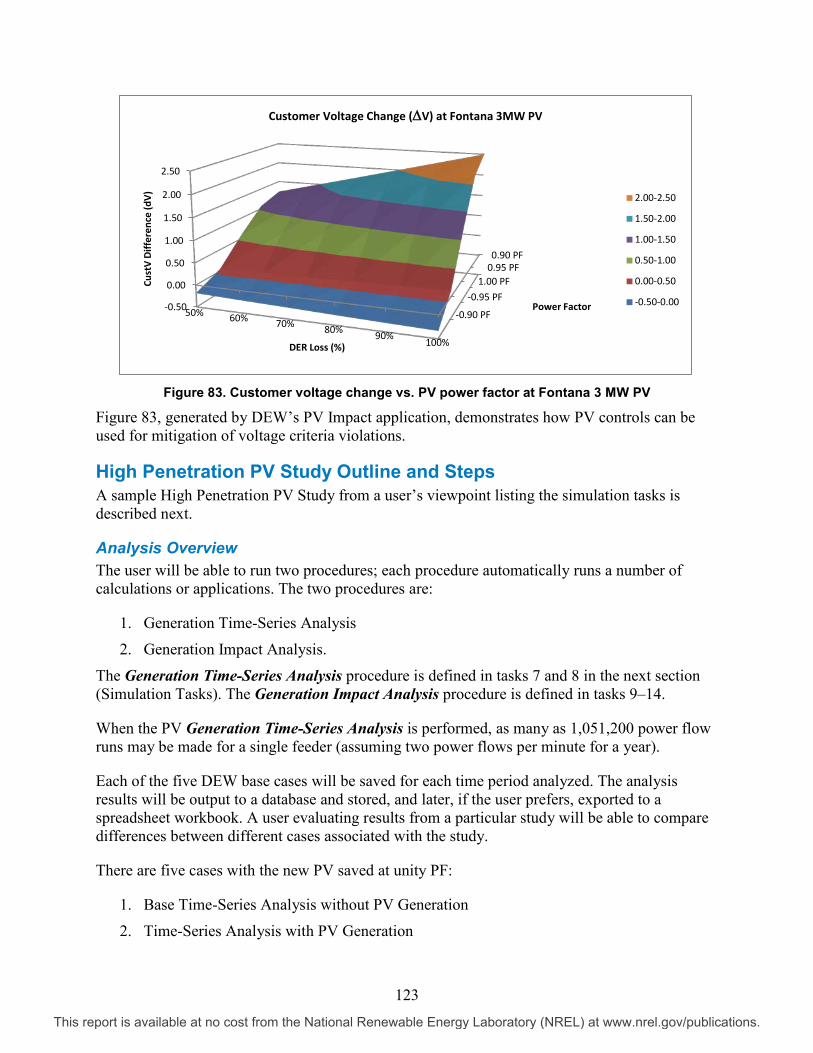
Figure 83. Customer voltage change vs. PV power factor at Fontana 3 MW PV

Figure 83, generated by DEW’s PV Impact application, demonstrates how PV controls can be used for mitigation of voltage criteria violations.

High Penetration PV Study Outline and Steps A sample High Penetration PV Study from a user’s viewpoint listing the simulation tasks is described next.

Analysis Overview The user will be able to run two procedures; each procedure automatically runs a number of calculations or applications. The two procedures are:

1. Generation Time-Series Analysis

2. Generation Impact Analysis.

The Generation Time-Series Analysis procedure is defined in tasks 7 and 8 in the next section (Simulation Tasks). The Generation Impact Analysis procedure is defined in tasks 9–14.

When the PV Generation Time-Series Analysis is performed, as many as 1,051,200 power flow runs may be made for a single feeder (assuming two power flows per minute for a year).

Each of the five DEW base cases will be saved for each time period analyzed. The analysis results will be output to a database and stored, and later, if the user prefers, exported to a spreadsheet workbook. A user evaluating results from a particular study will be able to compare differences between different cases associated with the study.

There are five cases with the new PV saved at unity PF:

1. Base Time-Series Analysis without PV Generation

2. Time-Series Analysis with PV Generation

-0.90 PF

-0.95 PF 1.00 PF

0.95 PF 0.90 PF

-0.50

0.00

0.50

1.00

1.50

2.00

2.50

50% 60% 70% 80% 90%100%

Power Factor

Cust

V Di

ffere

nce

(dV)

DER Loss (%)

Customer Voltage Change (∆V) at Fontana 3MW PV

2.00-2.50

1.50-2.00

1.00-1.50

0.50-1.00

0.00-0.50

-0.50-0.00

123


3. Impact Study at Rated Generation

4. Impact Study for Loss of Generation

5. Impact Study for Restoration of Generation.

The simulation tasks are described next.

Simulation Tasks Data Preparation

Task 1. For a new PV generator, normalize annual PV measurements with 1-minute sampling interval and store normalized curve in DEW Time-Series Storage. This curve is used to provide time-varying behavior for new PV installations to be evaluated.

Task 2. For the feeder to be analyzed, store start-of-feeder SCADA amp measurements

with 1-minute sampling interval into DEW Time-Series Storage. If only time-varying SCADA total power flow measurements are present, the power flow measurements will be converted to three-phase current measurements using sample measurements of feeder phase amps.

Task 3. Build a circuit model without PV generation, modeling all controller strategies

and settings, including time delays on controllers if time delays are greater than 1 minute.

Task 4. Validate circuit model without PV generation. Task 5. Model PV generation, including any control schedules. Task 6. Add PV and SCADA measurement associations to the model.

Begin Generation Time-Series Analysis Automated Procedure

Task 7. Use the graphical user interface (GUI) to specify feeder and PV components to analyze, specifying the name of the study. When analysis is started, Task 8 is performed automatically.

a. Perform 525,600 analysis sequences as indicated below, with two power flow runs per analysis sequence.

b. Perform base case power flow analysis (without PV generation) for next step in Time-Series Storage, where measurement matching is turned on. During the power flow analysis, if constraints on any component are violated, they shall be reported.

c. Set target loads (individual load points are now scaled to match start-of-circuit measurement without PV as a starting point for the next step to add PV). Note that an additional procedure is required if time-varying load distribution is not present and the use of connected kVA spot loads are used.

124


d. Perform power flow analysis with target loads, measurement matching turned off, and with PV generation for the same time step as in (a).

End Generation Time-Series Analysis Automated Procedure Begin Generation Impact Analysis Automated Procedure

Task 8. Use GUI to specify feeder and PV component to analyze, specifying the name of the study. When analysis is started, tasks 10–14 are performed automatically.

Task 9. Perform power flow analysis for all PV generation at rated capacity. Task 10. At peak daytime load with PV generation at rated capacity, perform power flow

analysis of loss of all PV generation, freezing all control devices. Task 11. Building on task 10 with all PV generation off, release control devices and

perform power flow analysis to achieve new controlled steady state. Then perform the next power flow analysis of restoration of all PV generation to rated capacity.

Task 12. At low daytime load, with PV generation at rated capacity, perform power flow

analysis of loss of all PV generation, freezing all control devices. Task 13. Building on task 12 with all PV generation off, release control devices and

perform power flow analysis to achieve new controlled steady state. Then perform the next power flow analysis of restoration of all PV generation to rated capacity before and after regulation.

End Generation Impact Analysis Automated Procedure

Task 14. Evaluate results, including the following:

a. Voltage profiles and differences in voltage profiles between cases

b. Maximum voltage variations for both daytime peak and low load conditions for both loss and restoration of rated generation. Report all instances of control devices at their regulating limits.

c. Counts of the number of annual operations of control devices along with estimated increase in automated line equipment annual operations

d. Islanding of generation including smallest amount of load isolated with generation

e. Back-feeding of line devices

f. System constraint violations

125


Begin Generation Fault Analysis Automated Procedure Task 15. User chooses points for analysis. This by default will be faults at the POI at PV

maximum and low daytime load, with PV generation at rated capacity. Choose all other protective devices or end of lines of interest and perform network fault analysis before PV and after PV.

Task 16. Save Generation Fault Analysis results to database.

The user will evaluate results for the initial screening (less than 10% of available system fault current) as well as interrupting ratings, min fault current desensitizing issues, fuse saving, and coordination.

Conclusions A detailed methodology for performing high penetration PV studies was developed. This included developing and testing proposed study criteria for evaluating the impacts of PV generation. These criteria were based on survey and evaluation of existing utility design standards. Criteria were used to evaluate impact of PV interconnection in terms of:


• High and low voltage constraints


• Expected impacts due to fault current contributions from the interconnected PV

• Additional operation of voltage control circuit elements

• Reverse flow. The developed study methodology and criteria were used to identify potential issues and to evaluate potential mitigation measures for resolving PV impact issues. Project work included development of visualization tools for measuring the extent and frequency of potential problems as well as comparing mitigation measures.

126


Overview of Fontana Area High Penetration Circuit Analysis This section provides an example of the methodology described above and applied to high penetration PV circuitry in the Fontana area.

Summary The high penetration PV analysis of the Fontana area circuit revealed two study criteria violations, both voltage issues. The first was high voltage over 126 meter volts at primary load-serving points in proximity to a capacitor bank; see Table 25. Investigation into the actual meter points and internal metering will help determine the cause of the high voltage. Note that the potential problem appears both with and without PV generation.

The second study criteria violation, a potential voltage rise or loss exceeding 0.7 meter volts, was observed at the PV POI for a PV system operating at unity PF for the 100% loss and return of rated PV; see Table 27 and Figure 83. In Table 27 it is apparent that a modification of the PV PF set point could resolve this study criteria violation. In addition, as seen in Table 30, it may be more realistic to consider a PV sudden loss and return of less than 100% of rated PV output.

Other significant results of note (although not study criteria violations) were the circuit’s reduction in capacitor switching and the improvement in circuit losses with the addition of PV.

Analysis Procedure The Fontana high penetration circuit analysis followed the procedure outline below, using the existing DEW functionality. This section’s discussion will also follow this outline.

• Base case model o Build the base case

o Model the active device controls

o Validate the base case

• Time-series input o Obtain circuit measurement data

o Obtain PV measurement input

• Validate the time-series model

o Identify data anomalies

o Fix/exclude bad data points

• Generation time-series analysis o Identify critical time points

o Quantify parameters of interest, annual behavior, and extent

• Generation impact analysis

127


o Run 24 hourly simulations over critical days identified by the time-series analysis

o Quantify effects of PV, its sudden loss and its return

• Generation fault analysis o Fault analysis with and without PV

• Summarize results and study criteria violations.

Base Case Model All necessary relevant data (as previously described) on the Fontana area circuitry were collected.

Quanta supplied a CYME model of the Fontana area circuitry—a one-line geographical circuit with the location of PV generators, type and size of the generators, and the settings of all capacitors.

A DEW model of the Fontana area 12 kV feeder was then built from the peak power flow circuit supplied by CYME. The CYME circuit model had a peak load for 2010 of 4.5 MVA, with a raw load PF of approximately 90%, and balanced three-phase loading. The load distribution was based on the transformer-connected kVA. The existing 2 MW PV1 was modeled operating at unity PF. Figure 84 shows the Fontana circuit modeled in DEW.

Figure 84. Fontana area circuit built within DEW.

DEW’s power flow was run on the model, and flows and voltages were compared to the CYME model power flow results with little or no differences noted.

Controls were then added to the capacitors.

The table below was provided for all the capacitor settings. Capacitors have two settings: slow trip is 2 minutes at moderate over/under voltages, and fast trip is for extreme situations at 5 seconds.

128


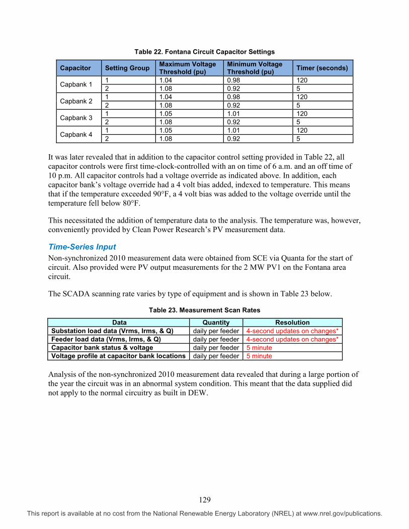
Table 22. Fontana Circuit Capacitor Settings

Capacitor Setting Group Maximum Voltage Threshold (pu)

Minimum Voltage Threshold (pu) Timer (seconds)

Capbank 1 1 1.04 0.98 120 2 1.08 0.92 5

Capbank 2 1 1.04 0.98 120 2 1.08 0.92 5

Capbank 3 1 1.05 1.01 120 2 1.08 0.92 5

Capbank 4 1 1.05 1.01 120 2 1.08 0.92 5

It was later revealed that in addition to the capacitor control setting provided in Table 22, all capacitor controls were first time-clock-controlled with an on time of 6 a.m. and an off time of 10 p.m. All capacitor controls had a voltage override as indicated above. In addition, each capacitor bank’s voltage override had a 4 volt bias added, indexed to temperature. This means that if the temperature exceeded 90°F, a 4 volt bias was added to the voltage override until the temperature fell below 80°F.

This necessitated the addition of temperature data to the analysis. The temperature was, however, conveniently provided by Clean Power Research’s PV measurement data.

Time-Series Input Non-synchronized 2010 measurement data were obtained from SCE via Quanta for the start of circuit. Also provided were PV output measurements for the 2 MW PV1 on the Fontana area circuit.

The SCADA scanning rate varies by type of equipment and is shown in Table 23 below.

Table 23. Measurement Scan Rates

Data Quantity Resolution Substation load data (Vrms, Irms, & Q) daily per feeder 4-second updates on changes* Feeder load data (Vrms, Irms, & Q) daily per feeder 4-second updates on changes* Capacitor bank status & voltage daily per feeder 5 minute Voltage profile at capacitor bank locations daily per feeder 5 minute

Analysis of the non-synchronized 2010 measurement data revealed that during a large portion of the year the circuit was in an abnormal system condition. This meant that the data supplied did not apply to the normal circuitry as built in DEW.

129


It was decided to gather and use synchronized 1-minute 2011 measurement data for the start of circuit. This was thought be sufficient because of the resolution of the SCADA data, and because it would match the 1-minute solar data. Clean Power Research provided synchronized 1-minute PV data for the 2 MW PV1.

From 2010 to 2011 the circuitry returned to its normal configuration. An expansion of the PV1 site from 2 MW to 3 MW was completed in December 2010. The 1.5 MW PV2 site was completed February 5, 2011.

The 1-minute 2 MW PV1 measurements provided by Clean Power Research were normalized, scaled, and used to produce 3 MW PV1 and 1.5 MW PV2 measurement datasets. These two sets of measurements were combined with the start-of-circuit measurements to determine the native load of the feeder. All the steady-state simulations in this study were performed using these measurements to provide scaling factors for the feeder’s load allocation, which was based on connected kVA from the original peak load base case. EDD prefers to use time-varying native load to determine the effects of PV, but the scaling factor method can be used as well—though it should be validated to make sure the load allocation is reasonable.

Validate the Time-Series Model Validation of the 2011 SCADA data input to the Time-Series Data revealed that the capacitor controls, as indicated above, and particularly the time clock controls, were not supported by the provided 1-minute data. Analysis of the 1-minute start-of-circuit measurements led to development of the capacitor control scheme shown in Table 24—this more closely represents the capacitor operation apparent in the measurement data.

Table 24. Approximated 2011 Capacitor Operation Base upon SCADA Measurements

Capacitor Configuration:

On Off

1: 1200 kVAr 6 a.m. 10 p.m. 2: 1800 kVAr 120.4V 126.2V 3: 1800 kVAr 121.2V 125.9V

Further validation of the measurement data revealed measurement anomalies (e.g., missing data, zeros) and spurious results (e.g., values not supported by the adjacent time points). This was true of the start-of-circuit data and to a lesser extent of the PV data. There are three ways to handle these data issues: obtain the right measurement, ignore the time point (if not a max or min value), or fix and fill the data. EDD chose to fix and fill the data by reviewing the previous minute, hour, or day. Please note that the number of anomalies was a very small fraction of the nearly 500,000 time points for analysis.

Run Generation Time-Series Analysis The Generation Time-Series Analysis was used to determine the Fontana native load profile by combining the start-of-circuit measurements with the coincident PV measurements. DEW’s existing DER Assessment dialog is shown in Figure 85. From this dialog, measurement data can be combined to determine native load, critical time point for DER impact analysis, and the impact of loss and restoration of PV generation.

130


Figure 85. DEW's DER Assessment dialog.

After determining the circuit native loading, the maximum and minimum native load (during daylight hours) time points were determined. Figure 86 illustrates the construction of the maximum load day. Figure 87 illustrates the construction of the minimum load day. Figure 88 illustrates the on to off peak load ratio, which symbolizes the enveloping conditions that the PV system will be operated within.

Figure 86. Peak day native load.

-1000

0

1000

2000

3000

4000

5000

6000

7000

8000

0 5 10 15 20 25

Peak ckt Meas

Peak ckt Load

Total PV

131


Figure 87. Minimum day native load.

Figure 88. On to off peak native load.

The hourly PV data were examined to determine the maximum PV output time. The maximum PV to load ratio and the maximum PV – load times were also determined. These five days became the study points for the initial PV impact detailed analysis:

• Maximum load day: 9/7/2011

• Minimum load day: 11/24/2011

• Maximum PV day: 6/26/2011

• Maximum PV to load ratio: 6/18/2011, .98

• Maximum PV – load day: 6/19/2011, -77 kW * statistically the same as 6/18/2011.

-500

0

500

1000

1500

2000

2500

3000

3500

4000

4500

5000

0 5 10 15 20 25

Total PV

Min ckt Meas

Min Ckt Load

0

1000

2000

3000

4000

5000

6000

7000

8000

0 5 10 15 20 25

Peak ckt Load

Min Ckt Load

132


The detailed analysis using 1-minute measurement data was used to define the following parameters of interest.

Table 25. Time-Series Analysis Customer Voltage Summary

Customer Voltage Summary : No PV With PV # of Primary Load Service Points with V > 126.0 for more than 0.5% of the year 15 9 # of Primary Load Service Points with V > 126.0 for more than 5% of the year 9 0 # of Primary Load Service Points with V > 126.5 for more than 0.2% of the year 8 0 # of Primary Load Service Points with V > 126.5 for more than 0.5% of the year 0 0 Min Cust V 118.8 119.2 Max Cust V 126.9 126.9 Max Volt was never > 127

Table 25 above reveals that the maximum customer-level voltage criterion has been violated. It appears that the high voltage is a function of the primary load service points being electrically close to circuit capacitor banks. It should be noted that all load service points were represented as primary load without distribution transformation. If these customers' meter points are on the secondary load service, they may not necessarily be experiencing high voltage. Detailed analysis during the mitigation phase should quantify this.

Table 26. Time-Series Capacitor Switching Summary

Table 26 summarizes the capacitor switching before PV1 and PV2 and with PV1 and PV2. By reviewing Table 26, it appears that the capacitor switching actually decreased. Note that we are assuming that the capacitor controls modified to match the start-of-circuit measurements were in effect before the PV was added in these time-series calculations.

No PV With PV Cap 1 Cap 2 Cap 3 Total Cap 1 Cap 2 Cap 3 Total Total Movement 668 17 335 1020 668 4 8 680 Jan Not analyzed Feb 56 3 14 73 56 2 58 Mar 62 6 24 92 62 62 Apr 60 4 43 107 60 60 May 62 50 112 62 2 64 Jun 60 41 101 60 60 Jul 62 2 40 104 62 2 2 66 Aug 62 2 32 96 62 2 2 66 Sep 60 40 100 60 60 Oct 62 27 89 62 62 Nov 60 19 79 60 60 Dec 62 5 67 62 62 Total switches (1 on and 1 off represents a count of 2)

133


The effect of power generation from the PV systems on circuit losses was examined.

• At peak, kW Flow: 8217 and kVAr Flow: -835 kVAr; the losses with no PV were (kW): 389.5

• With PV: kW Flow of 4620 and kVAr Flow: -1200 kVAr were (kW): 262.7. (Note: with the higher voltage due to the PV injection, the capacitors put out a lot more VARs).

Because PV generation is only contributing to circuit efficiency during daylight hours, the load factor method for comparing losses (because the PV is only helping the circuit efficiency during daylight hours) will produce inaccurate results. We ran analyses of 30-minute intervals for only February through December, and the losses in the “no PV” case were 1068 MWh; the losses during this period were 840 MWh. It thus appears that there is a loss benefit of at least 248 MWh. Using DEW’s efficiency program with locational marginal pricing for the Fontana commercial pricing node, we could quantify the economic benefit of the PV operation.

Generation Impact Analysis DEW was used to perform the Generation Impact Analysis simulations. These simulations were conducted for the 24-hour load cycle of each of the critical days listed above.

Normally we would expect the main impacts detected to be:

• Voltage rise or fall beyond operation limits

• Reverse power flows.

Also examined in this phase is imbalance, which should not be an issue with this balanced three-phase system.

The only criteria violation observed was an unregulated voltage rise above 0.7 V at the POI. EDD did not explicitly evaluate a series of potential mitigation alternatives, but it did examine a range of loss and rise of generation and various PFs for the inverter operation.

Table 27. Customer Voltage Change at POI vs. PV Power Factor

Power Factor

-0.90 PF -0.95 PF 1.00 PF 0.95 PF 0.90 PF

Fina

l DER

Lo

ss

50% -0.18 0.05 0.59 1.06 1.23 60% -0.22 0.07 0.72 1.28 1.48 70% -0.25 0.08 0.84 1.50 1.73 80% -0.28 0.10 0.96 1.72 1.99 90% -0.31 0.12 1.09 1.94 2.24 100% -0.33 0.14 1.22 2.16 2.50

Table 27 shows an output of DEW’s DER Impact Analysis, which demonstrates the impact of various loss of PV generation from rated output at various PV PF settings. It can be seen that limiting loss to only 60% of rated value at unity PF or modifying the PV PF would resolve this voltage drop criteria violation.

134


Table 28. Critical Time Point PV Impact Summary – Customer Voltage Variation with Varying PF

Table 28 was automatically generated by DEW’s DER Impact Analysis. This automatically generated output summarizes voltage deviation for all active elements, including all PV systems. It also summarizes those across a preselected range of PV control strategies.

Figure 89 shows how a user can review these results from within the GUI for any individual component. This will improve the ability of analysts to visualize and understand the impacts and possible mitigation alternatives.

135


Figure 89. Customer voltage at POI vs. PV power factor.

In Table 29, reverse flow at every active element is examined. Because the Fontana circuit has no active elements (e.g., transformer LTC, voltage regulators, or automatic protective devices), we elected to show all sectionalizing devices as an example of the reverse flow analysis methodology.

Table 29. Critical Time Point Analysis Reverse Flow Summary Component Info Max Difference

Name UID Type Time Phase kW Before (F1)

kW After (F2)

kW Difference

Unknown GS4897-2 Sectional Device Sep-07, 06:00 Phase A 6.49 6.50 0.01 Phase B 0.00 0.00 0.00 Phase C 0.00 0.00 0.00

Unknown B5505096S1 Sectional Device Sep-07, 06:00 Phase A 6.49 6.50 0.01 Phase B 0.00 0.00 0.00

Unknown 531E Sectional Device Sep-07, 11:00 Phase A 7.69 -900.49 -908.18 Phase B 7.74 -900.49 -908.22 Phase C 7.80 -900.46 -908.26

Unknown 0_1_324_4 Sectional Device Sep-07, 11:00 Phase A 0.00 -909.44 -909.44 Phase B 0.00 -909.44 -909.44 Phase C 0.00 -909.44 -909.44

Sectional device is not displayed unless there are some flow differences.

Reverse Flow Results (Sep 07 06:00 ~ 18:00) for Fontana Circuitry where F1: Real Flow (kW) with All Generation Off When Max Flow Difference Occurs F2: Real Flow (kW) with All Generation On When Max Flow Difference Occurs % Penetration = 100*(F1-F2)/F1

136


Another way to view the reverse flow data is depicted in Figure 90 below. In this figure, the DEW Fontana circuit has been colored using DEW’s variable range display to help visualize what circuit area has been affected by the PV.

Figure 90. Reverse flow visualization of Fontana.

No criteria violations are noted for reverse flow.

Table 30. 2011 Time-Series Analysis – PV Variability

PV Output – Minute-Over-Minute Variation Change in Output Loss of Output (instances) Gain in Output (instances)

> 1/3 of Rated Output 51 75 > 1/2 of Rated Output 17 15 >3/4 of Rated Output 0 0

In our PV impact analysis, we begin with an assumption of the 100% loss and gain of PV to define the variability impact of the PV on the circuit voltage. In Table 30, we have quantified the minute-over-minute PV variations. It appears that perhaps a less conservative value might be the 75% loss and return of PV. This revision to the PV impact analysis along with PF control revision to each PV may be used to determine mitigation strategies.

137


Generation Fault Analysis DEW’s Network Fault was run to determine if the PV installation would affect the protection system of the circuit. Table 31 below summarizes those results; we determined that the PV fault current was well below our screening criteria of 10%. In addition, the Fontana circuit as built has no protective devices internal to the circuit.

Table 31. Fault Current Summary

Location System Fault Current at the POI Without PV

PV Fault Current 1.1 x Full Load Ratio

3 MW PV 2250 160 7% 1.5 MW PV 2000 80 4%

138


Appendix A: Typical PV Database Needs

Typical Interconnection Application Information

Generation Information for Database

Generation Information (Photovoltaic Inverter Based)

Units Mandatory for Database?

Generator Manufacturer Model (Name/Number) Gross Nameplate Rating kVA y Net Nameplate Rating kW y AC Operating Voltage y Inverter Description kVA Rating kVA y kW Rating kW y Inverter Efficiency y Power Factor Rating y PF Adjustment Range y Rated Voltage Volts y Normal Operating Power Factor (%) Multiplier of Rated Current for Calculating Maximum Fault

Short-Circuit Current – 3-Phase Max 3-Phase Current as a Function of Voltage

y

3-Phase Winding Configuration – 3-Wire Delta, 3-Wire Wye, 4-Wire Wye

y

Neutral Grounding - Ungrounded, Grounded, Grounding Resistor in ohms

y

Neutral Grounding - Ungrounded, Grounded, Grounding Resistor in ohms

y

Short-Circuit Current – 3-Phase Max 3-phase current as a function of voltage

y

Isolating Transformer(s) between Generator(s) and Utility

Transformer Model Number Transformer Manufacturer Rated kV and Connection (delta, wye, wye-gnd) of Each Winding

y

kVA of Each Winding y BIL of Each Winding Fixed Taps Available for Each y

139


Winding Positive/Negative range for any LTC windings

%Z Impedance on Transformer Self-Cooled Rating

y

Percent Excitation Current at Rated kV

Load Loss Watts at Full Load or X/R Ratio

PV Site Installation Description Address, City, Zip (for cross checking)

Manufacturer Supplier Model Quantity (Number of

individual arrays)

Latitude (degrees) y Longitude (degrees) Tilt (degrees) Azimuth (degrees) Shading – 90 (East) (%) Shading – 120 (%) Shading – 150 (%) Shading – 180 (South) (%) Shading – 210 (%) Shading – 240 (%) Shading – 270 (West) (%) Inverter Description kVA Rating kVA y kW Rating kW y Rated Voltage Volts y Normal Operating Power Factor (%) Multiplier of Rated Current for Calculating Maximum Fault

Controlled? Quantity 1741 Qualified

140


Appendix B: Generation Impact Results Summary Form Level

Max/Min Date/Time of Level

Criteria Violation

No. of Instances

Notes Active Device

DER Assessment Summary

Screening: (Critical Time Points) Max Load Level and Time Low Load (daytime hours) Level and Time Max PV Level and Time Max PV to Load Ratio Level and Time Max Difference PV-Load Level and Time Highest Unregulated Voltage Rise at PCC/POI Sudden Loss of Rated PV

Lowest Unregulated Voltage Decrease at PCC/POI Sudden Return of Rated PV

Highest Unregulated Voltage Rise at Closest Active Device for Loss of Rated PV

Lowest Unregulated Voltage Decrease at Closest Active Device Sudden Return of Rated PV

Max Reverse kW at Vreg Level and Time (low load PV on)

Isc at PCC/POI without PV Isc of PV Detailed Full-Year Analysis Voltage Summary Elements Highest Customer Voltage Level and Time Lowest Customer Voltage Level and Time Highest Increase in Voltage at the POI, Active Devices

Highest Voltage at All Caps, Full PV Injection

Lowest Voltage at All Caps, 100% Loss of PV Injection

Active Device Movement Summary Capacitors Max Number of Movements per Day; Level and Date Before PV

Capacitors Max Number of Movements per Day; Level and Date with PV On

Movement of LTCs; Number per Year Before PV

Movement of LTCs; Number per Year After PV

Movement of Closest Vreg; Number per Year Before PV

Movement of Closest Vreg; Number per Year After PV

141


Reverse Flow Summary Elements Max Reverse Flow at Protective Devices Level and Time (any time)

Max Reverse Flow at Regulating Devices Level and Time (any time)

Overload Summary Worst Overload Caused by PV Level, Time And Location

Losses Annual Circuit Losses Without Normally Operated PV

Annual Circuit Losses with New PV Operating at Normally Expected Output

Time-Varying Solar Analysis Max PV Step Change Loss (e.g., Minute over Minute Gain in PV Output)

Max PV Step Change Gain (e.g., Minute over Minute Gain in PV Output)

Instances of loss of PV >50% but < Max PV (Step for the study time increment)

Instances of gain of PV >50% but < Min PV (Step for the study time increment)

142


Definitions ANSI C84.1: American National Standard for Electric Power Systems and Equipment. It establishes nominal voltage ratings for utilities to regulate the service delivery, and it establishes operating tolerances at the point of use.

CBEMA: Computer and Business Electronic Manufacturers Association (now International Committee for Information Technology Standards).

CBEMA Curve: Chart indicating voltage limits versus time of excursion from normal. Standard defining voltage limits for human perception/irritation and equipment operation.

The original CBEMA curve was developed by the CBEMA and adopted by IEEE Standard 446. CBEMA has been renamed as the Information Technology Industry (ITI) Council, and a new curve as shown below has been developed to replace the original CBEMA curve.

From http://whatispowerquality.blogspot.com/2012/02/cbema-and-itic-curves-power-quality.html. Clean Power Research (CPR): An organization whose services include providing irradiance data and power simulation for planning, developing and operating solar installations. Website: www.cleanpower.com.

Distributed Energy Resource (DER): Electric generation facilities connected to an area electric power system (EPS) through a point of common coupling (per IEEE 1547).

DER Assessment: An analysis using a system model to determine if the connection of a DER meets the host utility’s requirements. Outputs can be selected to identify voltage violations, overloads, excessive regulator movement, capacitor switching, and other problems. Along with other data, it provides maximum and minimum voltages and percentage of equipment loading capacity. It provides these values for maximum load conditions, minimum load conditions, and maximum PV generation. See Appendix B for more details.

Generation Fault Analysis: Fault current analysis to determine fault current magnitude and verify relay coordination and relay operation.

143


http://www.cleanpower.com/

Generation Impact Analysis: See DER Assessment.

IEEE 519: IEEE-519-1992 describes the recommended Practices and Requirements for Harmonic Control in Electrical Power Systems. The standard was first introduced in 1981 to provide direction on dealing with harmonics introduced by static power converters and other nonlinear loads so that power quality problems could be averted.

Max Native/Raw Load (Start of Circuit + PV Output) Time: The maximum circuit load if the solar was not there (which the utility is ultimately responsible for serving). Note that an outage will cause the loss of all PV for some time period after power is restored.

Max PV Output Time: Time at which all of the solar generation peaks independent of circuit load.

Min Load / Low Load Time Point: Daylight time when the native/raw circuit load is at its lowest.

Max PV Load Difference / Max Ratio of PV Output to Min Native Load Time Point: The ratio concept of a Min/Low load point or possibly a low load shoulder time.

Mitigation: Changes made to correct issues involved with the operation of the interconnected generation. Changes can include control set-points, equipment modification and/or replacement, and operational restrictions. Examples include modification to the operation of the generation, such as restricted output at certain times or system conditions. Changes could also include modification to the operation of the active elements on the circuit, or changes to the circuit configuration.

Native Load: Circuit, substation, or area load exclusive of any DERs providing power into the system.

Quasi-Steady-State: A related series of steady-state analyses intended to demonstrate the effects of a system with dynamic or changing conditions.

Reverse Power Flow: Power flow in the opposite direction of radial flow from substation to load, caused by the addition of one or more DERs.

Solar Irradiance: Power per unit area on the Earth's surface. It can be measured in watts/m2.

Solar Radiation: Energy sourced by the sun.

Time-Series Analysis: A series of power flow studies at uniform, specified time intervals intended to determine the time (and date) of maximum and minimum load, maximum generation, maximum ratio of generation to load, and other key electrical values pertinent to interconnection of generation.

Time-Series Storage: Storage of the files created by time-series analysis.

144


5 PV Interconnection Assessment for Fontana Circuit

145


Abstract This report is a companion report to Methods for Performing High Penetration PV Studies (Section 4 of this compilation report). The following report documents a PV mitigation strategy to resolve the voltage issues observed on the Fontana area circuitry. This mitigation strategy involves simply requiring the PV to be set to a fixed PF of .95 absorbing to resolve the voltage rise issue.

This report will outline other advanced inverter functionality that could be used to mitigate high penetration PV issues as well as utility measures that could be used to mitigate potential criteria violations.

146


Table of Contents Abstract .................................................................................................................................................... 146 List of Figures ......................................................................................................................................... 147 List of Tables ........................................................................................................................................... 147 Introduction ............................................................................................................................................. 148

Background ........................................................................................................................................ 148 Previous Study Results ....................................................................................................................... 149

High Penetration PV Mitigation Studies for Fontana .......................................................................... 151 Mitigation Strategies ............................................................................................................................... 153 Fontana Circuit Study – Conclusion ..................................................................................................... 154 Appendix A: PV Impact Results vs. Power Factor .............................................................................. 155

List of Figures Figure 91. Max voltage deviation vs. PV1 power factor. ..................................................................... 152 Figure 92. Max voltage deviation vs. PV2 power factor. ..................................................................... 152

List of Tables Table 32. Critical Time Point Analysis of Voltage Variation of 3 MW PV1 ........................................ 151 Table 33. Voltage Variation Analysis at Critical Time Points for 1.5 MW PV2 .................................. 151 Table 34. PV Output Minute-Over-Minute Variability ........................................................................... 153

147


Introduction This report documents mitigation strategies to resolve general issues with high penetration PV interconnection and, more specifically, voltage violations on the Fontana area high penetration PV circuitry.

The Fontana circuit was analyzed for impacts of high penetration PV interconnection in terms of:




• The impacts of implemented anti-islanding functions of the PV inverters

• The increase in the number of line regulator/switched capacitor bank operations caused by the interconnection of PV

• Other analysis discovered to be important to high penetration PV interconnection studies. Voltage regulation, i.e., managing the voltage rise and possible flicker issues, at the POI was the only problem observed.

This report also outlines the recommended advanced inverter functionality mitigation techniques for implementation, and suggests utility-side mitigation options.

Background One might think of connecting a PV system similarly to connecting a large motor load. In this case, the customer with the large motor load and its starting disturbance is responsible not to bother adjacent customers. The connection, starting, and operation of this large motor can be simulated and the interconnection can be facilitated with a number of very well-known and accepted techniques usually considered to be the responsibility of the motor owner. One might think of motor starting and operation similar to PV variability.

An advanced PV inverter, at near-zero marginal cost, could have the ability to virtually eliminate voltage variation on a distribution feeder due to variation in the real power output of a PV plant. The PV inverter could even mitigate the effects of load-induced voltage variations elsewhere on the feeder.

An advanced PV inverter could have the capability to mitigate the effect of its own variable real power output on the grid voltage by correcting changes while they are happening, maintaining dynamic VAr reserve in a similar way as is done in modern transmission-system VAr compensators.

As the criteria violations result from operation of the PV plant, it would seem appropriate that the PV plant would be primarily responsible for mitigating those problems. The first line of defense would be to require the PV source to mitigate the issues at its own terminals. This can be done by controlling the PV real and reactive outputs to the extent possible within the PV system’s existing capability. Next, one might consider modifying the PV system to have more

148


advanced control capabilities. Lastly, the utility may be able to modify its system without a detrimental effect to existing customers in such a way to accommodate the PV system. However, the PV system is usually responsible for the cost of those upgrades.

Mitigation measures at the PV system are analyzed here, such as inverter PF change. Mitigation may require both PV and utility actions.

Other mitigation measures for the utility to consider include requiring a separate feeder, requiring transfer trip, and revising existing equipment and its operation (e.g., revised settings for capacitor and regulator controls, relay settings, adding new components, and reconductoring and/or line extensions).

This report also outlines the recommended advanced inverter functionality mitigation techniques for implementation on the study feeder.

Previous Study Results In our previous report Methods for Performing High Penetration PV Studies, results for PV time-series analysis and PV impact studies revealed only a potential voltage variation problem at the POI for both PV1 3 MW and PV2 1.5 MW solar plants.

Analysis Overview In the previous study, two procedures were run, both with the constraint that each PV inverter was operating at unity PF. The two procedures were:

• Generation Time-Series Analysis

• Generation Impact Analysis.

Generation Time-Series Analysis The detailed analysis used 1-minute measurement data to define the following parameters of interest: circuit native loading, the maximum and minimum native load (during daylight hours), and the maximum PV day, which defines the enveloping conditions that the PV will be operated within.

These three days became the study points for the initial PV impact detailed analysis:

• Maximum load day: 9/7/2011

• Minimum load day: 11/24/2011

• Maximum PV day: 6/26/2011. Hourly data was also generated, by averaging 1-minute data, and used as input for each of the three critical days. From this analysis, the following critical time points were used as input to the Generation Impact Analysis.

149


Generation Impact Analysis DEW was used to perform the Generation Impact Analysis simulations. These simulations were conducted for the 24-hour load cycle of each of the critical days listed above.

The new PV operating at unity PF was analyzed at each of the four critical time points on the three critical enveloping days as indicated above. These time points are:




• Maximum difference between PV generation and native load.

For each time point, five cases were run as follows:

• Base Time-Series Analysis without PV Generation

• Time-Series Analysis with PV Generation

• Impact Study at Rated Generation

• Impact Study for Loss of Generation

• Impact Study for Restoration of Generation. A flicker or voltage rise criteria violation at the POI was noted and documented in the previous report. A potential voltage rise or loss of 0.7 meter volts was observed at the PV POI for each PV system operating at unity PF and considering the 100% loss and return of PV.

In DEW’s Generation Impact Analysis, the user may request to run a series of loss of generation and return of generation percentages to find what percentage of output causes a criteria violation to occur, and do this as a function of the inverter PF set point. This helps define at what point a criteria violation occurs and if there are PF set points that may help alleviate it.

This analysis was rerun for various loss and return percentages and at varying PFs. The simulation tasks were repeated from the original study conditions but this time using various PFs to determine a mitigation strategy.

150


High Penetration PV Mitigation Studies for Fontana The high penetration PV analysis of the Fontana area circuit revealed one study criteria violation. A potential voltage rise or loss of 0.7 meter volts was observed at the PV POI for a PV system operating at unity PF for the 100% loss and return of rated PV.

The DEW Generation Impact Application was run again, but this time over a range of PFs. These results are summarized in Table 32 and Table 33.

In the tables below, the impact of operating the PV generation on the critical days for 2011 is listed for the loss and return of 100% of the PV generation at each significant time points on those days. Further, each of those cases was rerun while varying the PV PF to lead us to a mitigation strategy. The summary results are shown in Table 32 and Table 33.

Table 32. Critical Time Point Analysis of Voltage Variation of 3 MW PV1 3 MW PV1 100% Loss and Return of PV Output

09/07/2011 11/24/2011 06/26/2011 Max (Peak) Load Day Min (Low) Load Day Max PV Day Analysis Time Points

PF = 1

PF = - .95 Absorbing

Table No

PF = 1


Table No

PF = 1


Table No

Max Load Time 0 1-1 1 0 1-2 1 0 1-3 Min Load Time 0 0 NA 0 0 NA 0 0 NA Max PV Time 1 0 1-4 1 0 1-5 1 0 1-6 Max Difference (Native Load - PV) Time

1 0 1-7 1 0 1-8 1 0 1-9

0 - Means no criteria violations 1 - Means criteria violation (voltage rise over 0.7 V on 120 V base)

Table 33. Voltage Variation Analysis at Critical Time Points for 1.5 MW PV2

1.5 MW PV2 100% Loss and Return of PV Output 09/07/2011 11/24/2011 06/26/2011 Max (Peak) Load Day Min (Low) Load Day Max PV Day Analysis Time Points

PF = 1 PF = - .95 Absorbing

Table No

PF = 1


Table No

PF = 1


Table No

Max Load Time

1 0 2-1 1 0 2-2 1 0 2-3

Min Load Time

0 0 NA 0 0 NA 0 0 NA

Max PV Time

1 0 2-4 1 0 2-5 1 0 2-6

Max Difference (Native Load - PV) Time

1 0 2-7 1 0 2-8 1 0 2-9

0 - Means no criteria violations 1 - Means criteria violation (voltage rise over 0.7 V on 120 V base)

151


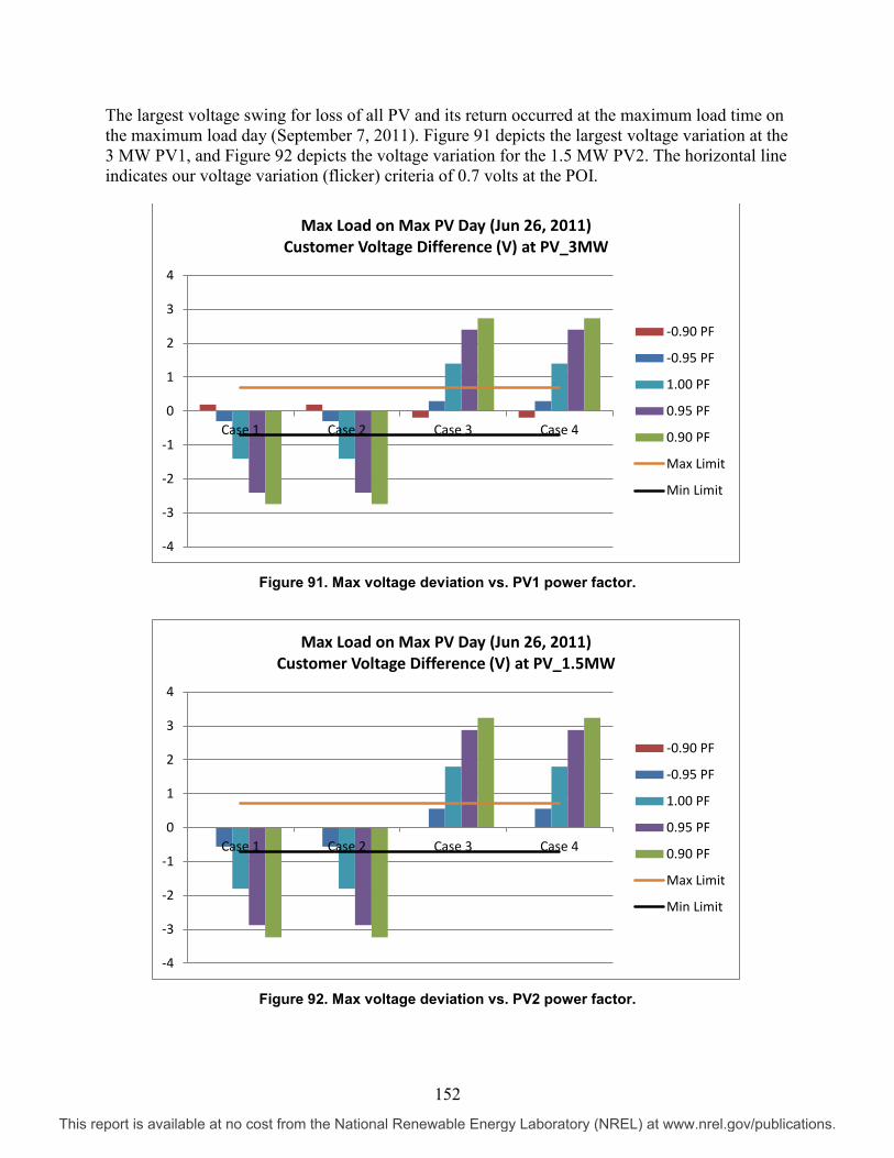
The largest voltage swing for loss of all PV and its return occurred at the maximum load time on the maximum load day (September 7, 2011). Figure 91 depicts the largest voltage variation at the 3 MW PV1, and Figure 92 depicts the voltage variation for the 1.5 MW PV2. The horizontal line indicates our voltage variation (flicker) criteria of 0.7 volts at the POI.

Figure 91. Max voltage deviation vs. PV1 power factor.

Figure 92. Max voltage deviation vs. PV2 power factor.

-4

-3

-2

-1

0

1

2

3

4

Case 1 Case 2 Case 3 Case 4

Max Load on Max PV Day (Jun 26, 2011) Customer Voltage Difference (V) at PV_3MW

-0.90 PF

-0.95 PF

1.00 PF

0.95 PF

0.90 PF

Max Limit

Min Limit

-4

-3

-2

-1

0

1

2

3

4

Case 1 Case 2 Case 3 Case 4

Max Load on Max PV Day (Jun 26, 2011) Customer Voltage Difference (V) at PV_1.5MW

-0.90 PF

-0.95 PF

1.00 PF

0.95 PF

0.90 PF

Max Limit

Min Limit

152


It is apparent that changing the PF set point to .95 absorbing will be sufficient to mitigate the criteria violation. Refer to Appendix A for a complete set of figures for each critical day and critical time point referenced in Table 32 and Table 33 and Figure 91 and Figure 92.

Table 34. PV Output Minute-Over-Minute Variability

PV Output – Minute-Over-Minute Variation Change in Output Loss of output (instances) Gain in output (instances) > 1/3 of Rated Output 51 75 > 1/2 of Rated Output 17 15 >3/4 of Rated Output 0 0

In our PV impact analysis, we begin with an assumption of the 100% loss and gain of PV to define the variability impact of the PV on the circuit voltage. In Table 34 above we have quantified the minute-over-minute PV variations. It appears that perhaps a less conservative value might be 75% (or less) loss and return of PV. This revision to the PV impact analysis along with PF control revision to each PV system may also be used to determine mitigation strategies.

Mitigation Strategies Three-phase inverters are the ultimate reactive power generators, capable of generating or absorbing high-quality reactive current that is controlled on an instantaneous basis. Modern inverters are unique in the world of VAr generators, because they are able to change their reactive power output extremely rapidly. Response times of the order of 1 ms to full output are achievable, which is very fast compared to other devices such as rotating synchronous condensers and other switched devices that use capacitors and inductors as the sources and sinks of reactive power. This fast response has allowed inverter-based VAr generators to be successfully applied for arc furnace flicker compensation and active power filtering, for example, where they operate in a sub-cycle control timeframe.

Inverters have the ability to provide real (P) and reactive (Q) output power simultaneously. By allowing intelligent control of real and reactive power, advanced inverters can help mitigate the effects of solar intermittency and improve power quality on the local distribution system. There are many ways in which these grid-smart power control features can be used for the benefit of the distribution system:

• Real power limits and real power ramp limits can be used to control the amount and rate of change of power delivered by distributed PV resources onto the distribution system.

• In PF Control Mode, the reactive power automatically tracks the real power output, maintaining a Q:P ratio that is consistent with the prevailing PF command. In PF Control Mode, the real power is limited below the inverter’s kVA rating if the PF is set to less than unity; i.e., real power would potentially be curtailed during periods of high PV production for PF < 1.

• In a Reactive Power Command Mode, the reactive power output follows a command up to the maximum available level. Reactive power is limited if it results in a PF greater than configured limits, or if it results in a value that exceeds the power limit of the drive. If the vector sum of the real and commanded reactive power exceeds the inverter’s kVA rating,

153


the reactive power is curtailed (i.e., real power takes precedence over reactive power). By setting the real power curtailment level below the inverter’s kVA rating, the inverter can also be configured to give the reactive power command precedence.

• In Voltage Compensation Mode, the inverter regulates the PF at the POI with a command proportional to the deviation of network voltage from a target set point.

• In Voltage Regulation Mode, the inverter seeks to regulate the inverter terminal to a target set point using its spare reactive power capability. Because this mode operates autonomously, it can respond very quickly to changes on the distribution system, and hence correct for intermittency-induced voltage instability more quickly than can conventional voltage regulators. Care must be taken when utilizing this option because it is a closed-loop function. It may not be possible for the inverter to actually drive the network voltage to the set point, which would result in the inverter residing at the limits of the controller for most of its operation.

Mitigation measures at the PV system are analyzed here, such as inverter PF change. Mitigation, in particular for minimum load, typically may require both PV and utility actions.

Other mitigation measures for the utility to consider include requiring transfer trip and revising existing equipment and its operation (e.g., revised settings for capacitor and regulator controls, relay settings, adding new components, and reconductoring and/or line extensions).

Fontana Circuit Study – Conclusion The only study criteria violations issue discovered during the High Penetration PV Study for the Fontana circuit was Voltage Rise/Fall with PV Variability. This voltage rise/fall issue can be mitigated by implementing a fixed PF setting of -0.95 absorbing (inductive). While this mitigation measure reduces Voltage Rise/Fall, it may necessitate oversizing of the PV inverter so as not to restrict the maximum PV output by 5% at times when it may otherwise be achievable.

154


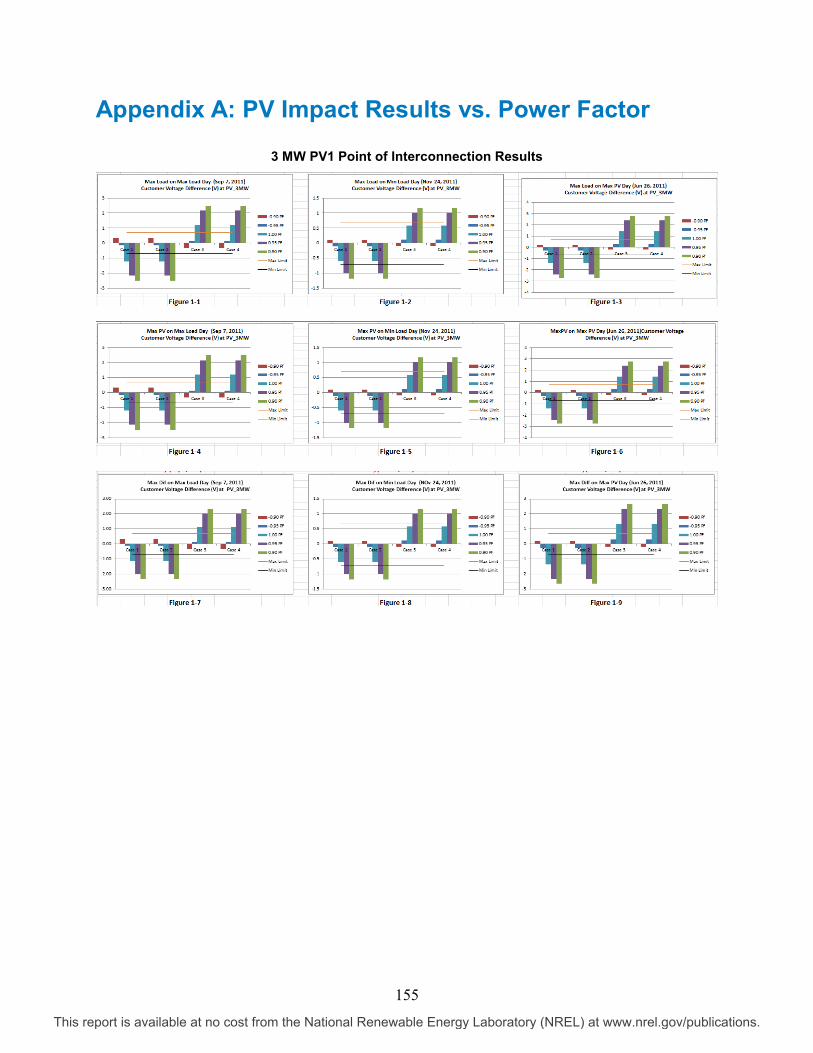
Appendix A: PV Impact Results vs. Power Factor

3 MW PV1 Point of Interconnection Results

155


1.5 MW PV1 Point of Interconnection Results

156


6 PV Interconnection Assessment for Porterville Circuit

157


Executive Summary The Porterville circuit with the existing 5 MW PV generation was modeled in the DEW suite of applications. The circuit impacts of adding the Porterville 5 MW PV are documented in this report. The assessment and potential impacts are presented along with possible mitigation strategies. A PV PF setting is suggested to mitigate a modest potential high voltage at the PV site and to reduce flicker due to PV variability.

Study Results EDD, using its DEW suite of analytic applications, found the following potential circuit-related issues associated with the operation of this PV:

• A modest potential overvoltage situation could exist on August 8, 2013, which could be resolved by applying a PF setting of -97.5% absorbing. Alternatively, if one is willing to accept the risk of having the PV slightly above 126 meter volts at the point of common coupling, when at full rated output, no other customer on the circuit should see a voltage above 126. Note that this observation assumed operating the Porterville circuit at 124 meter volts. A review of the SCADA start-of-circuit voltage revealed an average of 122.5 + 1.5 volts. If the circuit is operated at this voltage level, no overvoltage at light load is anticipated.

• A potential flicker (voltage rise or fall for sudden loss of PV generation) issue exists, which can be mitigated by applying a PF setting of -97.5% absorbing. Use of this PF setting should assure that the flicker would be no worse than the existing circuit capacitor switching voltage rise or fall. If a flicker level less than that of capacitors switching twice per day is required, a larger absorbing PF should be considered.

Note that an absorbing PF, e.g., -97.5% as indicated above, is used to offset voltage changes at the PV generator POI. When the PV real power (P) output rises, causing an increase in voltage, the PV absorbs an increasing amount of reactive power (Q) from the system, which will dampen that voltage rise. Conversely, when the PV real power output falls, causing a decrease in voltage, the PV will absorb a decreasing amount of reactive power from the system, which will dampen that voltage fall.

Circuit Recommendations It is suggested that a PF setting of -97.5% absorbing be considered to reduce flicker due to PV variability as well resolve a low-probability potential overvoltage.

158


Table of Contents Executive Summary ................................................................................................................................ 158

Study Results ...................................................................................................................................... 158 Circuit Recommendations .................................................................................................................. 158

List of Figures ......................................................................................................................................... 159 List of Tables ........................................................................................................................................... 159 Introduction ............................................................................................................................................. 160

Purpose ............................................................................................................................................... 160 Background ........................................................................................................................................ 160 Study Base .......................................................................................................................................... 162

Study Results .......................................................................................................................................... 170 Step Change Analysis ......................................................................................................................... 170 Variability Analysis ............................................................................................................................ 170 Active Device Movement ................................................................................................................... 174

Mitigation Recommendations ................................................................................................................ 175 Background ........................................................................................................................................ 175 High Penetration PV Mitigation Studies for Porterville ..................................................................... 176 Protection Review .............................................................................................................................. 179

Porterville Circuit Study – Conclusion ................................................................................................. 181 Appendix A: Study Violation Criteria .................................................................................................... 182 Appendix B: Listing of PV DER Assessment Violations on Porterville ............................................ 183

List of Figures Figure 93. DEW DER Assessment application. .................................................................................... 161 Figure 94. Porterville Sub Porterville circuit map. ............................................................................... 163 Figure 95. Specific day selection for the impact study in Porterville. ............................................... 166 Figure 96. Step change, PV setup. ........................................................................................................ 167 Figure 97. Specific Porterville DER Assessment – step change........................................................ 168 Figure 98. Scenario 1 for critical load days. ......................................................................................... 170 Figure 99. Porterville 5 MW PV site radiant variability analysis by minute. ...................................... 171 Figure 100. Porterville 5 MW PV site radiant variability analysis by hour. ....................................... 171 Figure 101. PV variability index and its histogram at maximum load day in Porterville. ................ 173 Figure 102. PV variability index and its histogram at minimum load day in Porterville. ................. 173 Figure 103. PV variability index and its histogram at maximum PV day in Porterville. ................... 173 Figure 104. Capacitor switching vs. % loss of PV. .............................................................................. 174 Figure 105. Capacitor switching vs. power factor. .............................................................................. 175 Figure 106. Voltage variations at the PV (UID_0_1_396_65) on maximum load day. ....................... 177 Figure 107. Voltage variations at the PV (UID_0_1_396_65) on minimum load day. ....................... 177 Figure 108. Voltage variations at the PV (UID_0_1_396_65) on maximum PV day. ......................... 178 Figure 109. Flicker vs. PV variability. .................................................................................................... 178 Figure 110. Flicker vs. PV power factor. ............................................................................................... 179

List of Tables Table 35. Porterville Circuit Capacitors and Control ........................................................................... 164 Table 36. Porterville Capacitor Flickers ................................................................................................ 164 Table 37. DER Impact Criteria ................................................................................................................ 169 Table 38. Porterville 5 MW PV Site Instance vs. % Variability vs. Time ............................................ 172 Capacitor Switching Violations at 100% Loss and Return of rated PV Output, Substation Regulated

to 122.5 .............................................................................................................................................. 183

159


Introduction Purpose The purpose of this study was to conduct a detailed analysis of the effects of operating a 5 MW PV system on the Porterville distribution circuit.

Background Study Methodology The distribution analysis tools used were DEW’s Power Flow, Network Fault Analysis, and DER Assessment applications. The DER Assessment application employs DEW’s time-series analysis capability with its quasi-steady-state power flow analysis and network fault analysis applications. These applications are used to quantify the impact of adding inverter PV generation as well as to determine mitigation measures for those impacts.

These studies included both steady-state and quasi-steady-state analysis, where quasi-steady-state analysis represents a series of analysis studies, such as power flow analysis, run over a set of time-varying measurement values. The quasi-steady-state power flow studies performed here can use either sample times of 1 second, 1 minute, or 1 hour. The results presented within primarily use 1-hour measurements because of the lack of measurements with higher sampling frequencies.

The impacts of the PV interconnection were analyzed in terms of:





• Other analysis discovered to be important to high penetration PV interconnection studies.

DER Assessment Overview DEW’s automated DER Assessment application was used to determine the impacts of adding DER to the system. The application dialog is shown in Figure 93.

160


Figure 93. DEW DER Assessment application.

The application has four tabs:

• The Fault Analysis tab determines fault current levels with and without PV. In this analysis, DEW’s Network Fault application is used to determine the fault current impacts of adding PV on circuit-level protection and coordination. This phase can also be used for analysis of ride-through settings. Fault analysis results are presented later in this report.

• The Step Change tab determines the potential impact of sudden changes in PV output on circuit criteria violations. The first phase of the assessment performed here uses hourly data.

• The Controller Movement tab uses available measurement data to estimate the movements of existing control equipment. This phase can be used to determine the extent of the circuit-level impacts of adding PV variability to the system or circuit. For more accurate results, this analysis requires minute/second data. The impact of PV on active device movement will be discussed later in this report.

• The Variability Analysis tab is used to create or define variability statistics from the actual measurement data to be used in the stepping analysis. Sufficient data were not available at the time to conduct this analysis.

The following discussion first covers the step change analysis, then the controller movement analysis, and finally the fault analysis.

161


To determine the impact of adding PV on the circuit, the study treated all of the PV systems on the circuit as a single source, from a solar variability perspective.

Step Change Background The DER Assessment should be performed over a whole year, using the most granular time-varying start-of-circuit and PV generation data available.

The application performs a series of power flow analysis runs associated with loss and restoration of user-selected PV generation and corresponding load conditions.

These corresponding conditions or critical time points for detailed analysis are automatically determined from the annual loading analysis. These time points may then be used in power flow analysis runs. A series of five distinct power flow runs are made for each critical time point selected for analysis:

• Base condition




• Return of generation with feeder controls operating. The above five power flows are run for each critical time point selected for analysis. There may be as many as five critical load/generation points:






The application automatically discovers the system’s active devices, and the series of power flows are run and all active device parameters are reviewed against the study criteria.

Study Base EDD worked together with NREL to provide an accurate DEW circuit model of the Porterville Feeder.

The existing Porterville circuit is a 12 kV distribution circuit approximately 40.7 miles in length. The planned peak load is 4600 kW for the 442 customer loads on the circuit. It has 5 MW of PV installed approximately 2.6 miles along the circuit. SCADA metering is available at the circuit head, and temporary metering (NREL distribution monitoring unit [DMU] and GridSense LT40) has been installed as well. Circuit voltage regulation is provided by four overhead capacitor banks. Protection is provided by the substation breaker; see Figure 94.

162


Figure 94. Porterville Sub Porterville circuit map.

DEW Model Build A flat file extract from CYME was received from NREL/SCE/Quanta for the Porterville base model, and a DEW circuit model was built. The load was represented by spot loads distributed throughout the circuit. Each spot load size was based on its value from the CYME model and a total load of 3600 kW with a native load PF of 96.16%. This became the base load at every load point in the circuit, which would be scaled by DEW measurement matching functionally for time-varying analysis.

Existing Circuit Regulation The circuit’s voltage is regulated to 122.5 + 1.5 meter volts.

In addition, there are four capacitor banks present with the control represented as shown in Table 35, controlled by a radio-activated time clock with voltage override. Note that the capacitor banks are biased to be always on during daylight hours.

163


Table 35. Porterville Circuit Capacitors and Control

The fastest operating time for the circuit regulation is 5 consecutive seconds for emergency voltages + 8% or 130 & 110 meter volt range, and 2 consecutive minutes for normal voltage excursions as listed in Table 35. A high / low voltage threshold is on the order of a 3-minute delay between switching operations.

Table 36. Porterville Capacitor Flickers

Capacitor Location Flicker on 120 V Base 600 kVAr Cap 13089 1.7 Volts 600 kVAr Cap 13903 0.7 Volts 600 kVAr Cap 13914 1.3 Volts 600 kVAr Cap 40409 2.8 Volts

Table 36 indicates the existing circuit flicker experience of the customers of the Porterville circuit caused by the daily switching of the capacitors, which are used for circuit voltage regulation.

Measurement Data When performing a DER Assessment, a year’s worth of measurement data should be used. The sampling rate should be inside (i.e., more frequent than) the typical utility operating times to determine voltage regulation issues. DEW’s quasi-steady state analysis can use time-series data at sub-1-second sampling times.

Measurement sets can be placed in DEW’s database for importing into DEW and attached to the circuit model. Measurements can be loaded at the measurement set sampling rate or at any higher sampling rate. Based upon the available measurement data, a blend of 1-minute and 1- hour measurement data was used for the study.

The following are examples of the available measurement data used to validate the circuit model so that the impacts of adding PV can be examined. Please refer to Figure 94 for meter locations.

• NREL DMUs are used to validate voltages at various points throughout the circuit.

• GridSense meters are a set of three-phase group meters at various points throughout the circuit with 1-second measurement values for current, phase angle, and PF.

o Group 7 can be used to establish current direction.

164


o Group 10 can be used to establish PV variability for 1 second, 1 minute, and 1 hour.

o Groups 6 and 9 can be used to validate the circuit flow proportions at major circuit splits.

• Clean Power Research 1-km 1-minute PV kW measurements are used to establish 1-minute variability (note that this was a point device capturing solar irradiance data for 2011).

• SCE EDNA SCADA data 1-hour extracted measurements o Start-of-circuit A phase current (no direction) and voltage

o PV generation MW and MVAr total.

Group 7 GridSense meters were used to determine three-phase start-of-circuit kW and kVAr and direction. Further, this measurement set was used to determine the critical time for the step change analysis.

Group 10 GridSense meters were used to determine the PV output. Group 10 meters did contain a small amount of load in addition to PV output, which was levelized and subtracted from the Group 10 measurement set. In addition, the SCE EDNA PV generation measurements were used to validate the Group 10 PV output.

Using the above set of measurements, the circuit native loading time points were determined for the maximum and minimum native load (during daylight hours) as well as the maximum PV.

Critical days from the 1-second 2013 GridSense meters:

• Max load day: 7/26/2013

• Max PV day: 8/5/2013

• Min load day: 9/2/2013.

Porterville Circuit Summary The impact study for the Porterville circuit 1-second resolution real and reactive power flow measurements at the start of the circuit and real power measurements at the PV system sites are used from 7/11/2013 to 9/11/2013. However, the PV measurements include the native load measurements, so it is difficult to separate the PV measurements without information on the native load. In this simulation, the PV measurements are generated by using real power measurement at start of the circuit. First, the native loads at start of the circuits are removed from the measurements, and then the dataset is scaled based on the PV rating. Therefore, its maximum generation is the same as the PV rating.

165


(a) Specific Time Selection For the impact study, the specific days are determined for evaluating the largest impacts on the circuit. The maximum and minimum load days are selected using the measurements at start of the circuit. However, it is difficult to select the maximum PV day because of mixed measurements. It is assumed that the measurements show more negative values when PV generation increases. The three days selected for the impact study as illustrated in Figure 95 are:

• Maximum circuit load: 7/26/2013

• Minimum circuit load: 9/2/2013

• Maximum PV generation: 8/5/201.

Figure 95. Specific day selection for the impact study in Porterville.

Figure 96 below shows the step up for determining the circuit’s native load from a combination of start-of-circuit measurements and PV output measurements. The PV can be part of the start of circuit or not included in the feeder measurement, as seen in Figure 96.

The entire Porterville 5 MW PV site will be considered to act together for analysis purposes.

166


Figure 96. Step change, PV setup.

167


Figure 97. Specific Porterville DER Assessment – step change.

As seen in Figure 97 above, there are five scenarios listed in the dialog, defined as follows:

Scenario 1 considers an initial PV output at 100% rated kW and unity inverter PF. There is a sudden loss of PV generation from 100% down to 0% output with all regulation frozen, then regulation is released after an appropriate time interval, then PV generation returns to 100% with all regulation frozen, and then regulation is again released to move after a time interval. This scenario is usually used first to define the areas of concern. If a circuit can withstand 100% loss of its PV generation without an issue, lesser and perhaps more probable variability should not be a major concern.

Scenario 2 repeats Scenario 1 only for the sudden loss of rated PV generation from 100% fully rated down to 20% (80% sudden loss of output), again at unity PF.


168



Scenario 5 repeats Scenario 1 only for the sudden loss of rated PV generation from 100% fully rated down to 80% (20% sudden loss of output) again at unity PF.

These scenarios are run on the critical or enveloping circuit loading conditions:

• Maximum native load day and hour

• Minimum native load day but maximum PV output hours

• Maximum PV day and hour. The DER Assessment application has a violation viewer used to view Scenario 1 results. An example can be seen in Figure 98 below. Note that this spreadsheet has various filters built in.

Figure 98 lists the following: analysis time points, feeders examined, active device, component types, and violation types. For each violation type, study criteria are established to measure the impact of the sudden stepping of the PVs. The power flow output is listed below. The output can be copied (e.g., to a spreadsheet), time points for power flow analysis can be automatically set, and all individual components can be panned to in DEW’s GUI.

Table 37 below lists the study variables used to measure the impact of the PV on the circuit. The user can chose his or her own violation study level. The criteria violation of interest was a 0.7 volt rise or fall at the PV POI that was observed (highlighted in Table 37).

Table 37. DER Impact Criteria

Initial Overvoltage Initial Undervoltage PV Step Down Overvoltage PV Step Down Undervoltage PV Step Up Overvoltage PV Step Up Undervoltage POI Initial Overvoltage POI Initial Undervoltage POI Step Down Overvoltage POI Step Down Undervoltage POI Step Up Overvoltage POI Step Up Undervoltage Step Down Voltage Change/Flicker Step Up Voltage Change/Flicker Step Down Controller Movement Step Up Controller Movement Step Down Voltage Change/Flicker Step Up Voltage Change/Flicker Step Down Controller Movement Step Up Controller Movement POI Voltage Change/Flicker (PV Step Down) POI Voltage Change/Flicker (PV Step Up) Reverse Flow

Detailed study criteria can be found in Appendix A.

169


Study Results Step Change Analysis

Figure 98. Scenario 1 for critical load days.

The initial step change analysis was made on the Porterville circuit by running Scenario 1, which considers the loss and return of PV output at 100% rated kW and unity inverter PF. This scenario is used first to define the areas of concern.

Potential circuit-related issues associated with the operation of this PV system versus our study criteria were found. See Figure 98 above for Scenario 1 study criteria failures.

A potential overvoltage situation of 126.4 meter volts was observed on August 8, 2013, for operation of the substation at 124 meter volts. However, a review of the SCADA start-of-circuit voltage revealed an average of 122.5 + 1.5 volts. When the study was revised to operate the start-of-circuit voltage at 122.5 volts, no overvoltage was observed. A potential flicker (voltage rise or fall for sudden loss of PV generation) greater than 0.7 volts was observed at the PV point of common coupling.

Detailed study results can be found in Appendix B.

Variability Analysis Point radiant solar 1-minute 1-km PV data for the Porterville site for 2011 was provided by Clean Power Research and was used initially to determine solar variability. The solar variability for the Porterville site is depicted in Figure 99 and Figure 100 and summarized in Table 38. The maximum variability days from the 2011 solar data from Clean Power Research are listed below.

• Maximum variability by minute: 7/3/2011, 12:00 at >90%

• Maximum variability by hour: 9/9/2011, 13:00 at 62%.

170


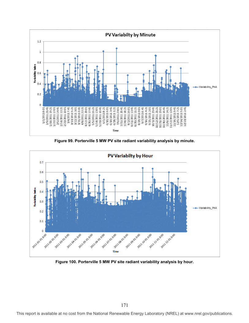
Figure 99. Porterville 5 MW PV site radiant variability analysis by minute.

Figure 100. Porterville 5 MW PV site radiant variability analysis by hour.

171


Table 38. Porterville 5 MW PV Site Instance vs. % Variability vs. Time

1 Minute Data (Instance) 1 Hour Data (Instance)

Total Instances 525600 8760 >90% variability 5 0 >80% variability 6 0 >70% variability 19 0 >60% variability 35 4 >50% variability 65 24 >40% variability 136 126 >30% variability 351 407 >20% variability 981 1546 >10% variability 3187 2854 >5% variability 7646 3597

The PV Variability Index is a measure of the PV power output changes over a selected sampling time interval as a ratio of total PV size as follows:

PV Variability Index = |𝑃𝑡−𝑃𝑡−∆𝑡|𝑃𝑟𝑎𝑡𝑖𝑛𝑔

where ∆𝑡 is the sampling time interval (1 second, 1 minute, and 1 hour), 𝑃𝑡 is the PV output at time t, and 𝑃𝑟𝑎𝑡𝑖𝑛𝑔 is the total PV size.

The radiant point data in Table 38 indicates a higher variability than was observed for 2013, which was actually metered from the aggregated 5 MW PV generation plant output. Measured variability of the entire 5 MW PV plant is listed below:

• Max variability by second: 8/17/2013 at 62%

• Max variability by minute: 8/6/2013 at 23%

• Max variability by hour: 7/13/2013 at 17%. Below is a listing of the variability analysis by critical or enveloping days for the actual PV plant. Different from the data shown in Table 38, which is a point device, Figures 87, 88 and 89 demonstrate how the variability is lower when spread over the entire PV area as opposed to a point source.

Figure 101, Figure 102, and Figure 103 show the PV variability index and its histogram at maximum load, minimum load, and maximum PV day, respectively. Most of the variability index is distributed less than 5% during all selected days. A few instances of a variability index of greater than 5% were observed with a maximum of approximately 40% for both the maximum and minimum load day. In the maximum PV day, a few instances of variability index are observed at more than 5% and with a maximum of approximately 18%.

172


Figure 101. PV variability index and its histogram at maximum load day in Porterville.

Figure 102. PV variability index and its histogram at minimum load day in Porterville.

Figure 103. PV variability index and its histogram at maximum PV day in Porterville.

173


Active Device Movement Under the Device Movement tab, the DER Assessment application uses available measurement data to estimate the change in movement of existing control equipment. This can be used to determine the extent of the circuit-level impacts of adding PV to the system or circuit.

The DER Assessment Device Movement tab will calculate device movement for a specific time period and at a specific time step. In the case of Porterville, insufficient data were available to support an accurate calculation of capacitor switching. However, the step change analysis from the previous section at the critical time points can give us a reasonable estimate as to the amount of switching.

Figure 104 below is an example of that step change analysis, which shows the potential switching for various losses and return of PV output. The analysis indicates that no additional capacitor switching would occur for loss of up to 40% of rated PV output. In fact, only the capacitor 40409, which is electrically close to the PV system, would operate for a 40% drop in PV output. Further, by reviewing the actual PV variability indicated in Figure 101, Figure 102, and Figure 103, which is predominately less than 40%, one can observe that no excessive switching would occur even at the critical or enveloping circuit conditions.

Figure 104. Capacitor switching vs. % loss of PV.

If some concern remains for the additional switching, Figure 105 below indicates that operating the PV at a fixed PF of -0.975 absorbing could also be used to reduce the number of switching operations.

174


Figure 105. Capacitor switching vs. power factor.

Mitigation Recommendations This section recommends advanced inverter functionality mitigation techniques and presents utility-side mitigation possibilities.

Background One might think of connecting a PV system similar to connecting a large motor load. In this case, the customer with the large motor load and its starting disturbance is responsible not to bother adjacent customers. The connection, starting, and operation of this large motor can be simulated and the interconnection can be facilitated with a number of very well-known and accepted techniques usually considered the responsibility of the motor owner. One might think of motor starting and operation similar to PV variability.

An advanced PV inverter, at near-zero marginal cost, could virtually eliminate voltage variation on a distribution feeder due to variation in the real power output of a PV plant. The PV inverter could even mitigate the effects of load-induced voltage variations elsewhere on the feeder.


As the criteria violation problems occur because of the PV plant, it would seem appropriate that the PV plant be primarily responsible to mitigate those problems. The first line of defense would be to require the PV source to mitigate the issues at its own terminals. This can be done by controlling the PV real and reactive outputs to the extent possible within the PV system’s existing capability. Next, one might consider modifying the PV system for a more advanced control.

175


The utility may elect to afford the PV system similar voltage excursions to those it would allow for a customer with a motor start, a capacitor switching voltage rise and fall—if no other detrimental effects are caused.

Lastly, the utility may be able to modify its system without a detrimental effect to existing customers in such a way to accommodate the PV system. However, the PV system is usually responsible for the cost of these upgrades.



High Penetration PV Mitigation Studies for Porterville Having found potential circuit-related issues associated with the operation of this PV system versus our study criteria, further analysis was conducted by modifying the step change to further quantify and sensitize the potential problems.

PV generation can use both active and reactive power injection for control. Fixed PF control can be considered and used to provide insights into the effect of the PF control, where the PFs considered in the simulations are given by:

• Case 1-1: 20% loss of generation, 0.8 absorbing PF


• Case 3-1: 20% loss of generation, 1.0 PF



• Case 3-2: 40% loss of generation, 1.0 PF



• Case 3-3: 60% loss of generation, 1.0 PF.

Generation Loss Power Factor 20% 40% 60% -0.8 Absorbing Case 1-1

100 - 80% Case 1-2 100 - 60%

Case 1-3 100 - 40%

-0.9 Absorbing Case 2-1 100 - 80%

Case 2-2 100 - 60%

Case 2-3 100 - 40%

1.0 Case 2-1 100 - 80%

Case 3-2 100 - 60%

Case 3-3 100 - 40%

176


Figure 106, Figure 107, and Figure 108 show the customer voltage variation at the PV system as a function of varying the PF of the PV generation for 20%, 40%, and 60% loss of generation, respectively. When the cases with same PF are compared, the voltage difference increases when increasing the loss of generation. When the cases with same loss of generation are compared, voltages decrease by using an increasing PV absorbing PF. When the cases with the same loss of generation are compared, voltages decrease by increasing lagging PF. Note that 0.9 absorbing PF control maintains a similar customer voltage level at the PV system—approximately at the value that existed before introducing loss of generation into the circuit. Furthermore, a 0.8 leading PF control can reduce the voltage level below that which existed prior to the introduction of the PV generation loss. These results provide information on PF control that can help mitigate voltage rise.

Figure 106. Voltage variations at the PV (UID_0_1_396_65) on maximum load day.

Figure 107. Voltage variations at the PV (UID_0_1_396_65) on minimum load day.

177


Figure 108. Voltage variations at the PV (UID_0_1_396_65) on maximum PV day.

The high penetration PV analysis of the Porterville circuit revealed one study criteria violation—a potential voltage rise or loss in excess of 0.7 meter volts, which was observed at the PV POI for a PV system operating at unity PF for the 100% loss and return of rated PV.

The DEW Generation Impact application was run again, only this time over a range of PFs. These results are summarized in Figure 109 and Figure 110.

Figure 109. Flicker vs. PV variability.

178


Figure 110. Flicker vs. PV power factor.

The modest potential overvoltage situation can be managed by continuing operation of the substation to the 122.5 volts actually observed for the sudden loss of 100% of fully rated PV output at unity PF.

The flicker (voltage rise or fall for sudden loss of PV generation) issue can be mitigated by applying a PF setting of -97.5% absorbing. Use of this PF should assure that the flicker would be no worse than the existing circuit capacitor switching voltage rise or fall. If a flicker level less than that of capacitors switching twice per day is required, a larger absorbing PF should be considered.

Protection Review Fault protection is provided from the breaker at Porterville Substation, which is equipped with three type CO-6 electromechanical phase relays and one type CO-8 electromechanical ground relay. Relay settings and associated timing curves are provided in the appendix.

Impedance at substation:

R+ X+ R0 X0 Provided P. U. Z at 100 MVA 0.08423 0.51525 0.00000 0.46667 Ohms at 12 kV (= P.U. Z *12kV2/100MVA) 0.12129 0.74196 0.00000 0.67200

179


Fault currents at substation with PV on:

1PhZ0FA PhToPhFA 3PhZ0FA 9870.4 8252.9 9504.1 9870.4 8252.9 9504.1 9870.4 8252.9 9504.1 Fault Currents at substation with PV off:

1PhZ0FA PhToPhFA 3PhZ0FA 9581.7 7980.8 9215.4 9581.7 7980.8 9215.4 9581.7 7980.8 9215.4 Fault current at the first switch is reduced to a maximum of 8002 amperes. Note that expulsion link fuses typically have an interrupting rating of 8000 amperes. The maximum is near this value. Caution should be used in installing this type of fuse on any devices closer to the substation than this first overhead switch.

1PhZ0FA PhToPhFA 3PhZ0FA 7330.1 6930.2 8002.3 7330.1 6930.2 8002.3 7330.1 6930.2 8002.3 Fault currents provided by the PV at the POI (288 amperes, three-phase) are greater than 10% of the fault current provided by the substation at the POI. More detailed review is warranted for fault currents greater that 10% of that provided by the substation.

Fault currents at the PV without PV on:

1PhZ0FA PhToPhFA 3PhZ0FA 750.7 1159.1 1338.4 750.7 1159.1 1338.4 750.7 1159.1 1338.4 Fault currents at the PV with the PV on:

1PhZ0FA PhToPhFA 3PhZ0FA 1005.1 1410.2 1602.8 1005.1 1410.2 1602.8 1005.0 1410.2 1602.8 Note the additional three-phase fault current of 264 amperes (1602–1338).

This is based on a 1.2 factor for maximum current contribution for an inverter with an aggregate of 5 MVA (1.2*5 MVA/(12 kV*sqrt(3)) = 289 amperes.

180


For some laterals, the operation of the substation breaker will be slower due to the infeed current supplied by the inverter. Some improved protection can be provided by additional sectionalizing fuses. For example, a sectionalizing fuse or recloser should be considered for the laterals that extend to the furthest north point and the furthest northwest points on the circuit.

Operating Sequence for Faults No protective devices have been indicated for line sectionalizing. Therefore, all faults must be cleared by operation of the substation breaker.

Fault Currents With the PV operating, fault current at the POI of the new PV is 1602 amperes three-phase and 1005 amperes phase-to-ground.

With the PV off, three-phase fault currents range from 9215 amperes at the substation to 875 amps at the remote northwest end of the circuit. Trip time for three-phase faults by the substation breaker is approximately 2 seconds.

If the PV continues to provide 1.2 times rated current into the fault at the remote northwest end, the trip time can be slowed to approximately 3 seconds depending on the load on the system. Standard undervoltage protection for anti-islanding should be installed to trip the PV off and shorten the trip time by the substation breaker. Further improvement can be achieved by installing a transfer trip scheme to trip the PV for operation (opening) of the substation breaker.

Porterville Circuit Study – Conclusion The only study criteria violation issue discovered during the high penetration PV study for the Porterville circuit was voltage rise/fall with PV variability. This voltage rise/fall issue can be mitigated by implementing a fixed PF setting of -0.95 absorbing. While this mitigation measure reduces the voltage rise/fall, it may necessitate the oversizing of the PV inverter so as not to restrict the maximum PV output by 5% at times when it may otherwise be achievable.

181


Appendix A: Study Violation Criteria Criteria Possible Study Limit Comments Device Movement Capacitor Switching Change in number of operations

with and without PV e.g., capacitor switching <6 times per day

Depends on type of control, no. of operations per day/year Note capacitor switching may actually be reduced


Depends on bandwidth, no. of operations per day/year



Voltage Impacts High Voltage – 126 V e.g., 126 V Or local utility customers’ maximum Low Voltage – 114 V e.g., 114 V Or local utility customers’ minimum Flicker at Active Element

e.g., 0.5 V Approx. 25% of active element voltage bandwidth

Flicker at PCC/POI e.g., 0.7 V Threshold of visual perception Overload Normal ratings All devices day-to-day or normal ratings Reverse Flow No back feed

182


Appendix B: Listing of PV DER Assessment Violations on Porterville

Flicker Violations at 100% Loss and Return of Rated PV Output

Overvoltage Violations at 100% Loss and Return of Rated PV Output, Substation Regulated to 124

Capacitor Switching Violations at 100% Loss and Return of Rated PV Output, Substation

Regulated to 124

Capacitor Switching Violations at 100% Loss and Return of rated PV Output, Substation Regulated

to 122.5

183


Appendix C: Relay Setting Details Porterville relay settings as provided:

3) Porterville Circuit

Relay => Phase = CO Inv. (CO-6) & Ground = CO Very Inv. (CO-8)

CT = 400/5

a) Phase

Tap = 6 A (480 amps primary)

Timing = 1.4 seconds at 16 amps secondary (1280 amps primary)

b) Ground

Tap = 1.0 A (80 amps primary)

Timing = 1.0 seconds at 8 amps secondary (640 amps primary)

Porterville Settings Comments:

This timing of the phase relay requires a time dial of about 4.5.

This timing of the ground relay requires a time dial of about 3.6 to 3.7.

184


Time-Current Curves for ABB CO-6 Relay

185


Time-Current Curves for ABB CO-8 Relay

186


7 PV Interconnection Assessment for Palmdale Circuit

187


Executive Summary The Palmdale circuit with the existing 3 MW PV generation was modeled in DEW. The circuit impacts associated with the operation of the two Palmdale 1.5 MW PV systems are documented in this report. The assessment and potential impacts are presented along with possible mitigation strategies. A PV PF setting is suggested for mitigation to reduce flicker because of potential PV variability.

Study Results EDD, using its DEW suite of analytic applications, found the following potential circuit-related issues associated with the operation of the Palmdale PV.

A potential flicker (voltage rise or fall for sudden loss of PV generation) issue exists, which can be mitigated by applying a PF setting of -97.5% absorbing. It is recommended that a -97.5% absorbing PF setting be used to limit the infrequent flicker to be the same as that of a switching capacitor bank for a sudden loss of as much as 80% of rated PV output. Use of this PF should assure that the flicker would be no worse than switching a circuit capacitor.

Note that an absorbing PF, e.g., -97.5% as indicated above, is used to offset voltage changes at the PV generator point of interconnection. When the PV real power (P) output rises, causing an increase in voltage, the PV inverter absorbs an increasing amount of reactive power (Q) from the system, which will dampen that voltage rise. Conversely, when the PV real power (P) output falls, causing a decrease in voltage, the PV inverter will absorb a decreasing amount of reactive power (Q) from the system, which will dampen that voltage fall.

Circuit Recommendations It is suggested that a PF setting of -97.5% absorbing be considered to reduce flicker due to PV variability.

188


Table of Contents Executive Summary ................................................................................................................................ 188

Study Results ...................................................................................................................................... 188 Circuit Recommendations .................................................................................................................. 188

List of Figures ......................................................................................................................................... 189 List of Tables ........................................................................................................................................... 189 Introduction ............................................................................................................................................. 190

Purpose ............................................................................................................................................... 190 Background ........................................................................................................................................ 190 Study Base .......................................................................................................................................... 192

Study Results .......................................................................................................................................... 199 Step Change Analysis ......................................................................................................................... 199 Variability Analysis ............................................................................................................................ 200 Active Device Movement ................................................................................................................... 201

Mitigation Recommendations ................................................................................................................ 202 Background ........................................................................................................................................ 202 High Penetration PV Mitigation Studies for Palmdale ....................................................................... 203 Protection Review .............................................................................................................................. 207

Palmdale Circuit Study – Conclusion ................................................................................................... 209 Appendix A: Study Violation Criteria .................................................................................................... 210 Appendix B: Listing of PV DER Assessment Violations on Palmdale .............................................. 211

List of Figures Figure 111. DEW DER Assessment application. .................................................................................. 191 Figure 112. Palmdale circuit map. ......................................................................................................... 193 Figure 113. Specific day selection for the impact study in Palmdale. ............................................... 195 Figure 114. Specific Palmdale DER Assessment – step change. ...................................................... 196 Figure 115. Step change, PV setup. ...................................................................................................... 197 Figure 116. Scenario 1 for critical load days. ....................................................................................... 199 Figure 117. PV variability index and its histogram on maximum load day for Palmdale. ............... 200 Figure 118. PV variability index and its histogram on minimum load day for Palmdale. ................ 201 Figure 119. PV variability index and its histogram on maximum PV day for Palmdale. .................. 201 Figure 120. Voltage variations at the Palmdale PV on maximum load day. ...................................... 204 Figure 121. Voltage variations at the Palmdale PV on minimum load day. ...................................... 204 Figure 122. Voltage variations at the Palmdale PV on maximum PV day. ........................................ 204 Figure 123. Flicker vs. PV variability vs. PV power factor. ................................................................. 205 Figure 124. Flicker vs. PV power factor. ............................................................................................... 206

List of Tables Table 39. DER Impact Criteria ................................................................................................................ 198

189


Introduction Purpose The purpose of this study was to conduct a detailed analysis of the effects of operating the two 1.5 MW PV systems on the Palmdale distribution circuit.

Background Study Methodology The distribution analysis tools used were DEW’s Power Flow, Network Fault Analysis, and DER Assessment applications. The DER Assessment application employs DEW’s time-series analysis capability with its quasi-steady-state power flow analysis and network fault analysis applications. These applications are used to quantify the impact of adding inverter PV generation as well as to determine mitigation measures for those impacts.

These studies included both steady-state and quasi-steady-state analysis, where quasi-steady-state analysis represents a series of analysis studies, such as power flow analysis, run over a set of time-varying measurement values. The quasi-steady-state power flow studies performed here can use either sample times of 1 second, 1 minute, or 1 hour. The results presented within primarily use 1-hour measurements because of the lack of measurements with higher sampling frequencies.

The impacts of the PV interconnection were analyzed in terms of:




• Expected impacts due to fault current contributions from the interconnected PV systems

• Other analysis discovered to be important to high penetration PV interconnection studies.

DER Assessment Overview DEW’s automated DER Assessment application was used to determine the impacts of adding DER to the system. The application dialog is shown in Figure 111.

190


Figure 111. DEW DER Assessment application.

The application has four tabs:

• The Fault Analysis tab determines fault current levels with and without PV. In this analysis, DEW’s Network Fault application is used to determine the fault current impacts of adding PV on circuit-level protection and coordination. This phase can also be used for the analysis of ride-through settings. Fault analysis results are presented later in this report.

• The Step Change tab determines the potential impact of sudden changes in PV output on circuit criteria violations. The first phase of the assessment performed here uses hourly data.

• The Controller Movement tab uses available measurement data to estimate the movements of existing control equipment. This phase can be used to determine the extent of the circuit-level impacts of adding PV variability to the system or circuit. For more accurate results, this analysis requires sub-minute data. The impact of PV on active device movement will be discussed later in this report.

• The Variability Analysis tab is used to create or define variability statistics from the actual measurement data to be used in the stepping analysis. There was not sufficient data available at the time to conduct this analysis.

The following discussion first covers the step change analysis, then the movement analysis, and finally the fault analysis.

191


To determine the impact of adding PV on the circuit, the study treated all of the PV systems on the circuit as a single source, from a solar variability perspective.

Step Change Background The DER Assessment should be performed over a whole year, using the most granular time-varying start-of-circuit and PV generation data available.

The application performs a series of power flow analysis runs associated with loss and restoration of user-selected PV generation and corresponding load conditions.

These corresponding conditions or critical time points for detailed analysis are automatically determined from the annual loading analysis. These time points may then be used in power flow analysis runs. A series of five distinct power flow runs are made for each critical time point selected for analysis:

• Base condition




• Return of generation with feeder controls operating. The above five power flows are run for each critical time point selected for analysis. There may be as many as five critical load/generation points:






The application automatically discovers the system’s active devices, and the series of power flows are run and all active device parameters reviewed against the study criteria.

Study Base Existing Palmdale Circuit This circuit is a 12 kV distribution circuit approximately 14.6 miles in length with a peak load of 3600 kW and 19,120 kVA of connected transformer capacity. Sixteen customers are on the circuit. The circuit line is depicted in Figure 112.

192


Figure 112. Palmdale circuit map.

Existing Circuit Regulation The Palmdale circuit’s voltage is regulated to 122.5 + 1.5 meter volts. There are no capacitors present on the circuit to provide internal circuit regulation.

DEW Model Build A flat file extract from CYME was received from NREL/SCE/Quanta for the Palmdale base model, and a DEW circuit model was built. The load was represented by spot loads distributed throughout the circuit. Each spot load size was based on its value from the CYME model. This became the base load at every load point in the circuit and was scaled by DEW measurement matching functionally for time-varying analysis.

This model was verified and brought up to date using the overhead operating circuit one-line diagram provided by SCE/Quanta. Once the earlier DEW model updates were completed, power flow converged on the model.

Temporary metering (NREL DMU and GridSense LT40) has been installed as well. Protection is provided by the substation breaker; see Figure 112.

193


Measurement Data When performing a DER Assessment, a year’s worth of measurement data should be used. The sampling rate should be inside (i.e., more frequent than) the typical utility operating times to determine voltage regulation issues. DEW’s quasi-steady-state analysis can use time-series data at sub-1-second sampling times.

Measurement sets can be placed in DEW’s database for importing into DEW and attached to the circuit model. Measurements can be loaded at the measurement set sampling rate or at any higher sampling rate. Based on the available measurement data, a blend of 1-minute and 1-hour measurement data was used for the study.

The following are examples of the available measurement data used to validate the circuit model so that the impacts of adding PV can be examined. Please refer to Figure 112 for meter locations.

NREL DMU Data – used to validate voltages at various points throughout the circuit.

Palmdale_P5625634: These are the transformer numbers at which the DMUs are located; this one is located at the end of the eastern lateral, the easternmost part of the circuit.

Palmdale_P5544436: These are the transformer numbers at which the DMUs are located; this one is located inside the PV plant, one of the main transformers the PV plants connect to.

Palmdale_P5625676: These are the transformer numbers at which the DMUs are located; this one is near the end of the circuit on the northwestern-most part.

GridSense Monitors LT40 – sets of three-phase group meters at various points throughout the circuit with 1-second measurement values for current, phase angle, and PF.

201305 Group 8 – P12421903_201 Phase 1, 2, 3: This unit is located on the short lateral used to connect the PV systems; it measures the PV system output current.

201305 Group 11 – P12422904 Phase 1, 2, 3: This unit is located on the first lateral heading east on the circuit, near PS 0420; it measures the loading of the entire lateral headed east

201305 Group 12 – P12423902 Phase 1, 2, 3: This unit is located right outside the substation near PS 0455; bi-directionality of this unit's current requires using the PF/angle to determine current flow direction, i.e., the current is a scalar value.

Group 8 GridSense meters were used to determine the PV output and to establish PV variability for 1 second, 1 minute, and 1 hour.

Group 11 GridSense meters were used to validate the circuit flow proportions at major circuit splits.

Group 12 GridSense meters were used for determining three-phase start-of-circuit kW, kVAr, and direction. Further, this measurement set was used to determine the critical time for the step change analysis.

Using the above set of measurements, the circuit native loading time points were determined for the maximum and minimum native load (during daylight hours) as well as Max PV.

194


Critical days from the 1-second 2013 GridSense meters:

• Max load day: 7/26/2013

• Max PV day: 8/5/2013

• Min load day: 9/2/2013.

Palmdale Circuit Summary The impact study for the Palmdale circuit used 1-second resolution real and reactive power flow measurements at the start of the circuit and real power measurements at the PV for the 5/11/2013 to 8/31/2013 time period.

(a) Specific time selection For the impact study, the specific days are determined for evaluating the largest impacts on the circuit. The maximum and minimum load days are selected using the measurements at start of the circuit. However, it is difficult to select the maximum PV day because of mixed measurements. It is assumed that the measurements show more negative values when PV generation increases. The three days selected for the impact study, as illustrated in Figure 113, are:

• Maximum circuit load: 8/23/2013

• Minimum circuit load: 7/5/2013

• Maximum PV generation: 6/23/2013.

Figure 113. Specific day selection for the impact study in Palmdale.

Figure 114 below shows the step up for determining the circuit’s native load from a combination of start-of-circuit measurements combined with the PV output measurements. The PV can be part of the start of circuit or not included in the feeder measurement, as seen in Figure 115.

The entire Palmdale 3 MW PV generation (two sites) will be considered to act together for analysis purposes.

195


Figure 114. Specific Palmdale DER Assessment – step change.

196


Figure 115. Step change, PV setup.

As can be seen in Figure 114 above, five scenarios are listed in the dialog, defined as follows:

Scenario 1 considers an initial PV output at 100% rated kW and unity inverter PF. There is a sudden loss of PV generation from 100% down to 0% output with all regulation frozen, then regulation is released after an appropriate time interval, then PV generation returns to 100% with all regulation frozen, and then again regulation is released to move after a time interval. This scenario is usually used first to define the areas of concern. If a circuit can withstand 100% loss of its PV generation without an issue, lesser and perhaps more probable variability should not be a major concern.





These scenarios are run on the critical or enveloping circuit loading conditions:

• Maximum native load day and hour

• Minimun native load day but maximum PV output hours

• Maximum PV day and hour.

197


The DER Assessment application has a violation viewer used to view Scenario 1 results. An example can be seen in Figure 116 below. Note that this spreadsheet has various filters built in.

Figure 116 lists the following: analysis time points, feeders examined, active device, component types, and violation types. For each violation type, study criteria are established to measure the impact of the sudden stepping of the PVs. The power flow output is listed below. The output can be copied (e.g., to a spreadsheet), time points for power flow analysis can be automatically set, and all individual components can be panned to in DEW’s GUI.

Table 39 below shows the study variables used to measure the impact of the PV on the circuit. The user can chose his or her own violation study level. The criteria violation of interest was a 0.7 volt rise or fall at the PV POI that was observed (highlighted in Table 39).

Table 39. DER Impact Criteria Initial Overvoltage Initial Undervoltage PV Step Down Overvoltage PV Step Down Undervoltage PV Step Up Overvoltage PV Step Up Undervoltage POI Initial Overvoltage POI Initial Undervoltage POI Step Down Overvoltage POI Step Down Undervoltage POI Step Up Overvoltage POI Step Up Undervoltage Step Down Voltage Change/Flicker Step Up Voltage Change/Flicker Step Down Controller Movement Step Up Controller Movement Step Down Voltage Change/Flicker Step Up Voltage Change/Flicker Step Down Controller Movement Step Up Controller Movement POI Voltage Change/Flicker (PV Step Down) POI Voltage Change/Flicker (PV Step Up) Reverse Flow

Detailed study criteria can be found in Appendix A.

198


Study Results Step Change Analysis

Figure 116. Scenario 1 for critical load days.

The initial step change analysis was made on the Palmdale circuit by running Scenario 1, which considers the loss and return of PV output at 100% rated kW and unity inverter PF. This scenario is used first to define the areas of concern.

Potential circuit-related issues associated with the operation of the PV generation versus our study criteria were found. See Figure 116 above for Scenario 1 study criteria failures. The only study criteria violation of note is a potential flicker (voltage rise or fall for sudden loss of PV generation) greater than 0.7 volts at the PV point of common coupling.

Detailed study results can be found in Appendix B.

199


Variability Analysis PV Variability Index is a measure of the PV power output changes over a selected sampling time interval as a ratio of total PV size as follows:

PV Variability Index = |𝑃𝑡−𝑃𝑡−∆𝑡|𝑃𝑟𝑎𝑡𝑖𝑛𝑔

where ∆𝑡 is the sampling time interval (1 second, 1 minute, and 1 hour), 𝑃𝑡 is the PV output at time t, and 𝑃𝑟𝑎𝑡𝑖𝑛𝑔 is the total PV size.

Below is a listing of the variability analysis by critical or enveloping days for the actual PV plant. The data shown in Figure 117, Figure 118, and Figure 119 demonstrate how the variability is lower when spread over the entire PV area as opposed to when calculated for a point source.

Figure 117, Figure 118, and Figure 119 show the PV variability index and its histogram at maximum load, minimum load, and maximum PV day, respectively. Most of the variability index is distributed less than 5% during all selected days. On the maximum load day, a variability index of greater than 5% was not observed and its maximum was approximately 2.5%, as shown in Figure 117. A few instances of a variability index greater than 5% are observed with a maximum of approximately 14% for the minimum load day. A few instances of variability index are observed between 5% and 10% for the maximum load day with a maximum of approximately 9%. Therefore, most of the second variability during the day is less than 5%, and its maximum is around 10%.

Figure 117. PV variability index and its histogram on maximum load day for Palmdale.

200


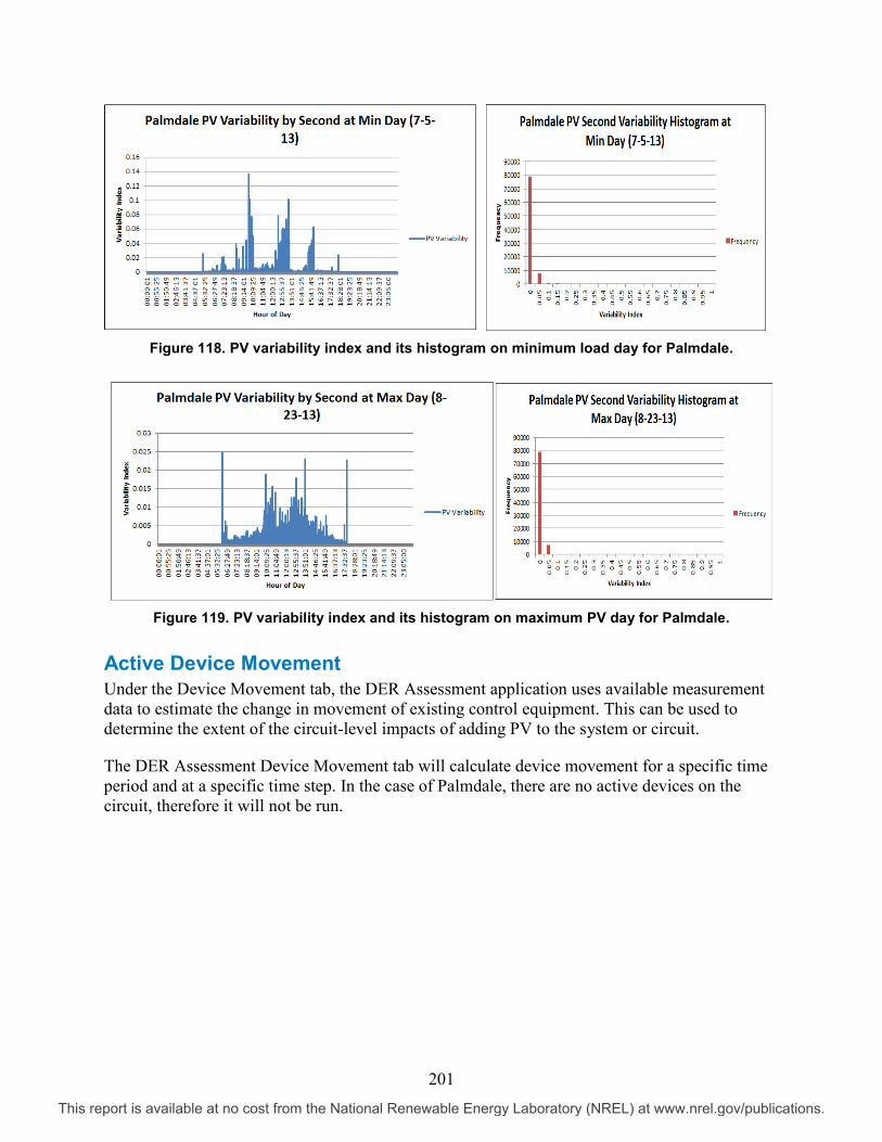
Figure 118. PV variability index and its histogram on minimum load day for Palmdale.

Figure 119. PV variability index and its histogram on maximum PV day for Palmdale.

Active Device Movement Under the Device Movement tab, the DER Assessment application uses available measurement data to estimate the change in movement of existing control equipment. This can be used to determine the extent of the circuit-level impacts of adding PV to the system or circuit.

The DER Assessment Device Movement tab will calculate device movement for a specific time period and at a specific time step. In the case of Palmdale, there are no active devices on the circuit, therefore it will not be run.

201


Mitigation Recommendations This section recommends advanced inverter functionality mitigation techniques and presents utility-side mitigation measures. Background One might think of connecting a PV system similar to connecting a large motor load. In this case, the customer with the large motor load and its starting disturbance is responsible not to bother adjacent customers. The connection, starting, and operation of this large motor can be simulated and the interconnection can be facilitated with a number of very well-known and accepted techniques usually considered the responsibility of the motor owner. One might think of motor starting and operation similar to PV variability.

An advanced PV inverter, at near-zero marginal cost, could virtually eliminate voltage variation on a distribution feeder due to variation in the real power output of a PV plant. The PV inverter could even mitigate the effects of load-induced voltage variations elsewhere on the feeder.


As the criteria violation problems occur because of the PV plant, it would seem appropriate that the PV plant be primarily responsible to mitigate those problems. The first line of defense would be to require the PV source to mitigate the issues at its own terminals. This can be done by controlling the PV real and reactive outputs to the extent possible within the PV system’s existing capability. Next, one might consider modifying the PV system for a more advanced control.

The utility may elect to afford the PV system similar voltage excursions to those it would allow for a customer with a motor start, a capacitor switching voltage rise and fall—if no other detrimental effects are caused.

Lastly, the utility may be able to modify its system without a detrimental effect to existing customers in such a way to accommodate the PV system. However, the PV system is usually responsible for the cost of those upgrades.



202


High Penetration PV Mitigation Studies for Palmdale Having found potential circuit-related issues associated with the operation of this PV system verses our study criteria, further analysis was conducted by modifying the step change to further quantify and sensitize the potential problems.

PV generation can use both active and reactive power injection for control. Fixed PF control can be considered and used to provide insights into the effect of the PF control, where the PFs considered in the simulations are given by:

Case 1-1: 20% loss of generation, 0.8 absorbing PF


Case 3-1: 20% loss of generation, 1.0 PF



Case 3-2: 40% loss of generation, 1.0 PF



Case 3-3: 60% loss of generation, 1.0 PF.

Generation Loss

Power Factor 20% 40% 60% -0.8 Absorbing Case 1-1

100 - 80% Case 1-2 100 - 60%

Case 1-3 100 - 40%

-0.9 Absorbing Case 2-1 100 - 80%

Case 2-2 100 - 60%

Case 2-3 100 - 40%

1.0 Case 2-1 100 - 80%

Case 3-2 100 - 60%

Case 3-3 100 - 40%

Figure 120, Figure 121, and Figure 122 show the customer voltage variation at the PV system as a function of varying the PF of the PV generation for 20%, 40%, and 60% loss of generation. When the cases with the same PF are compared, the voltage difference increases when increasing the loss of generation. When the cases with the same loss of generation are compared, voltages decrease by using an increasing PV absorbing PF. Note that 0.9 absorbing PF control maintains a similar customer voltage level at the PV system—approximately at the value that existed before introducing loss of generation into the circuit. Furthermore, a 0.8 absorbing PF control can reduce the voltage level below that which existed prior to the introduction of the PV generation loss. These results provide information on PF control that can help mitigate voltage rise.

203


Figure 120. Voltage variations at the Palmdale PV on maximum load day.

Figure 121. Voltage variations at the Palmdale PV on minimum load day.

Figure 122. Voltage variations at the Palmdale PV on maximum PV day.

204


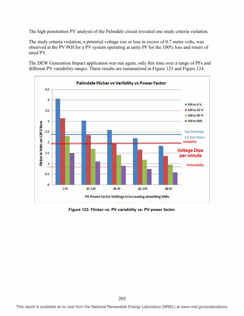
The high penetration PV analysis of the Palmdale circuit revealed one study criteria violation.

The study criteria violation, a potential voltage rise or loss in excess of 0.7 meter volts, was observed at the PV POI for a PV system operating at unity PF for the 100% loss and return of rated PV.

The DEW Generation Impact application was run again, only this time over a range of PFs and different PV variability ranges. These results are summarized in Figure 123 and Figure 124.

Figure 123. Flicker vs. PV variability vs. PV power factor.

205


Figure 124. Flicker vs. PV power factor. The flicker (voltage rise or fall for sudden loss of PV generation) issue can be mitigated by applying an absorbing PF setting at the PV. The amount of absorbing PF would depend on the allowable flicker to other customers. If a 600 kVAr capacitor bank were installed on the end of the Palmdale circuit for voltage regulation, it would produce a 2.4 volt flicker. Using a 92.5% absorbing PF setting at the PV should assure that the flicker would be no worse than a circuit capacitor switching voltage rise or fall. If a flicker level less than that of capacitors switching twice per day is required, a larger absorbing PF should be considered.

In addition, by reviewing the PV variability in Figure 117, Figure 118, and Figure 119, a lower absorbing PF setting could be used. Particularly recognizing that these are two separate facilities even though they are physically and electrically close, there may be some diversity in their variability.

It is recommended that a -97.5% absorbing PF setting be used to limit the infrequent flicker to be equal to that of a switching capacitor bank for a sudden loss of as much as 80% of rated PV output.

206


Protection Review Impedance at substation:

R+ X+ R0 X0 Provided P. U. Z at 100 MVA 0.06634 0.38614 0.00000 0.21567 Ohms at 12 kV (= P.U. Z *12kV2/100MVA) 0.09553 0.55604 0.00000 0.31056

Substation Fault currents at substation with west and east PVs on:

1PhZ0FA PhToPhFA 3PhZ0FA 14686.1 10841.0 12486.2 14686.1 10841.0 12486.2 14686.1 10841.0 12486.2 Fault currents at substation with both PVs off:

1PhZ0FA PhToPhFA 3PhZ0FA 14479.9 10634.8 12280.0 14479.9 10634.8 12280.0 14479.9 10634.8 12280.0 Fault current at the first switch is 10092 amperes. The fault current does not fall below 8000 amperes until a point on the 4720 foot line section (ACSR_336 UID 771321E$ND15756487) after the first switch. Typical interrupting capability for universal link fuses is 8000 amperes. Interrupting capability should be checked for protective devices on this section or closer to the substation.

Fault currents at first switch:

1PhZ0FA PhToPhFA 3PhZ0FA 11400.0 8767.5 10092.0 11400.0 8767.5 10092.0 11400.0 8767.5 10092.0

207


West PV Fault currents provided by the west inverter at the POI (103 amperes, three-phase) are less than 10% of the fault current provided by the substation at the POI. Typically, ratios below 10% do not adversely affect protective relaying.

Fault currents at the west PV without any PV on:

1PhZ0FA PhToPhFA 3PhZ0FA 1449.1 1884.1 2175.6 1449.1 1884.1 2175.6 1449.1 1884.1 2175.6 Fault currents at the west PV with the west PV on:

1PhZ0FA PhToPhFA 3PhZ0FA 1552.2 1987.2 2278.7 1552.2 1987.2 2278.7 1552.2 1987.2 2278.7 For some laterals, the operation of the substation breaker will be slower due to the infeed current supplied by the inverter. For a three-phase fault at the end of the lateral furthest east, contribution from the west PV will increase the trip time slightly from 1.57 seconds to 1.73 seconds. This is due to the smaller contribution (981 amperes vs. 1043 amperes) from the substation. Some improved protection can be provided by additional sectionalizing fuses. For example, a sectionalizing fuse or recloser should be considered for the lateral that extends to the furthest east point on the circuit.

208


East PV Fault currents provided by the PV at the POI (103 amperes, three-phase) are less than 10% of the fault current provided by the substation at the POI. Typically, ratios below 10% do not adversely affect protective relaying.

Fault currents at the east PV without any PV on:

1PhZ0FA PhToPhFA 3PhZ0FA 1509.8 1974.2 2279.7 1509.8 1974.2 2279.7 1509.8 1974.2 2279.7 Fault currents at the east PV with the east PV on:

1PhZ0FA PhToPhFA 3PhZ0FA 1612.9 2077.3 2382.8 1612.9 2077.3 2382.8 1612.9 2077.3 2382.8 Similar to the west PV, for some laterals, the operation of the substation breaker will be slower due to the infeed current supplied by the inverter. Some improved protection can be provided by additional sectionalizing fuses. For example, a sectionalizing fuse or recloser should be considered for the lateral that extends to the furthest east point on the circuit.

See Appendix C for relay setting details.

Palmdale Circuit Study – Conclusion The only study criteria violations issue discovered during the high penetration PV study for the Palmdale circuit was voltage rise/fall with PV variability. This voltage rise/fall issue can be mitigated by implementing a fixed PF setting of -95% absorbing. While this mitigation measure reduces the voltage rise/fall, it may necessitate the oversizing of the PV inverter so as not to restrict the maximum PV output by 5% at times when it may otherwise be achievable.

209


Appendix A: Study Violation Criteria Criteria Possible Study Limit Comments Device Movement Capacitor Switching Change in number of operations

with and without PV e.g., Capacitor switching <6 times per day

Depends on type of control, no. of operations per day/year Note capacitor switching may actually be reduced





Voltage Impacts High Voltage – 126 V e.g., 126 V Or local utility's customer maximum Low Voltage – 114 V e.g., 114 V Or local utility's customer minimum Flicker at Active Element

e.g., 0.5 V Approx 25% of active element voltage bandwidth

Flicker at PCC/POI e.g., 0.7 V Threshold of visual perception Overload Normal Ratings All devices day-day or normal ratings Reverse Flow No Back Feed

210


Appendix B: Listing of PV DER Assessment Violations on Palmdale

Flicker Violations at Various Scenarios – Loss and Return of Rated PV Output

Flicker Violations at Various Scenarios – Loss and Return of Rated PV Output at Various Power Factor Settings

Flicker Violations at Various Scenarios – Various Loss and Return of Rated PV Output at Various Power Factor Settings

211


Appendix C: Relay Setting Details Palmdale relay settings as provided: 2) Palmdale Relay = GE F35 CT = 800/5 a) Phase

Curve = IAC Very Inverse Tap = 0.375 pu (300 amps primary) Timing = 3.75 [0.65 seconds at 18 amps secondary (2880 amps primary)]

b) Ground

Curve = IAC Very Inverse Tap = 0.113 pu (90 amps primary) Timing = 3.02 [0.5 seconds at 5.63 amps secondary (900 amps primary)]

Palmdale Settings Comments: Note the “Tap” is the multiplier for the 800 amp rating of the CT 0.375 x 800 = 300 0.113 x 800 = 90.5

212


GE IAC Very Inverse Time-Current Curves

213


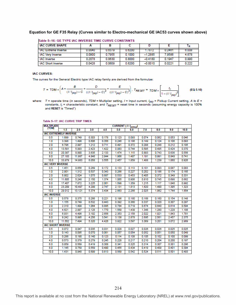
Equation for GE F35 Relay (Curves similar to Electro-mechanical GE IAC53 curves shown above)

214


Spreadsheet Results for GE F35 Relay

Ipkp I Tdm A B C D E TrVery Inverse Constants: Phase 300 2880 3.75 0.09 0.796 0.1 -1.29 7.959 4.678

Grnd 90 900 3.02Phase T= 0.632784Grd T= 0.499536

215


nrel/sce high penetration pv integration project: …€¢ lab testing of advanced pv inverter...

Documents