nonlinear differential equations with deviating … · nonlinear differential equations with...
TRANSCRIPT
Electronic Journal of Differential Equations, Vol. 2017 (2017), No. 68, pp. 1–25.
ISSN: 1072-6691. URL: http://ejde.math.txstate.edu or http://ejde.math.unt.edu
NONLINEAR DIFFERENTIAL EQUATIONS WITH DEVIATINGARGUMENTS AND APPROXIMATIONS VIA A
PARKER-SOCHACKI APPROACH
VINCENZO M. ISAIA
Abstract. The Parker-Sochacki method has been successful in generating ap-
proximations for a wide variety of ODEs, and even PDEs of evolution type,
by achieving an autonomous polynomial vector field and implementing thePicard iteration. The intent of this article is to extend PSM to a large fam-
ily of differential equations with deviating arguments. Results will be given
for problems with delays which are linear in time and state independent, andalso have constant initial data and nonlinear differential equations which are
retarded, neutral or advanced. The goal of the proofs is to motivate a numeri-cally efficient DDE solver. In addition, an explicit a priori error estimate that
does not require derivatives of the vector field is presented. The non-constant
initial data cases and the state dependent delay cases are discussed formally.
1. Introduction
In 1964, Fehlberg [6] produced a technical report for NASA that touched uponthe benefits of auxiliary variables in solving ODEs. This idea appeared to gounnoticed and in 1989 Parker and Sochacki noticed the benefit of a polynomialenvironment for the Picard iteration, whose integral form both preserves the poly-nomial environment as well as computes the appropriate Taylor polynomial for theanalytic solution on its domain.
The method of Parker and Sochacki was introduced in [9] and the structure ofthe class of ODEs was studied in [3]. The method was extended to PDEs in [10]and an explicit a priori error estimate, which do not rely on derivatives of thevector field in the ODE case, was given in [13] , see also [11]. The method wasdubbed the PS method in [12], here the acronym PSM is used. This method asapplied to ODEs will be reviewed in Section 2, along with the presentation of anarray interpretation that will be applicable in the deviating argument case and anexample which converts a non-polynomial and non-autonomous vector field to anautonomous, polynomial one.
After establishing an existence and uniqueness result via the method of successiveapproximations in Section 3, the central intent of this article is to adapt PSM tocertain nonlinear differential equations with deviating arguments, referred to asDDEs, whose initial data is polynomial. This approach, dubbed dPSM, is presented
2010 Mathematics Subject Classification. 34K07, 34K40, 65L03.Key words and phrases. Delay differential equations; lag; PSM method; method of steps;
method of successive approximation; deviating argument.c©2017 Texas State University.
Submitted April 1, 2016. Published March 8, 2017.
1
2 V. M. ISAIA EJDE-2017/68
in Section 4. In addition, two examples are presented, one that converts a DDE’svector field to an autonomous, polynomial one and another that highlights a specialcase of how information can propagate.
In the case of linear in time and state independent delays, structures for theapproximation to the solution across time can be established, and this is done inSection 5. The purpose of highlighting these structures is so they can be lever-aged computationally. To understand the structure across iterations, which canalso provide computational benefit, the array approach from Section 2 for PSM isdeveloped in Section 6 for dPSM.
Two more examples are also given in Section 6, one that looks more carefullyat converting vector fields, since this process is not unique, along with an examplethat shows how ‘’lag’ dependence appears and propagates in the coefficients of thepolynomial series approximation. The proof of the structure across iterations aswell as explicit a priori error bounds that do not rely on higher order derivativesof the vector field. A formal discussion occurs in Section 8 concerning the use ofdPSM for state dependent delays.
2. PSM overview
Given an initial value problem or IVP, based on a scalar ODE, the introductionof a polynomial vector field to the method of successive approximation allows thePicard iteration to be viewed as more than just a theoretical tool. If the Picarditeration can be shown to converge, establishing existence and uniqueness of asolution to the IVP, then a polynomial vector field will preserve the polynomialform of the initial data, which is constant, for all iterations, and a structure arisesthat allows the coefficients of the polynomial to be computed efficiently. In additionto requiring a polynomial form, the vector field also needs to be autonomous and theproblem begun at time t0 = 0, which can be achieved when t0 6= 0 via the changet = t − t0 since d
dt = ddt . Picard’s then generates a Maclaurin polynomial, and
shifting the time variable recovers the required Taylor polynomial of the solution.An autonomous polynomial vector field requires the introduction of auxiliary
variables that replace non-polynomial terms with polynomial terms, where nonlin-earity and non-autonomous terms are exchanged for a larger system size. It can beshown that the analytic functions that arise as (a component of the) solutions toan ODE with a polynomial vector field, occupies a large portion of the class of allanalytic functions, although they are not equal, see [3]. The solution of an ODEwhose vector field can be transformed into a polynomial one, is dubbed projectivelypolynomial. The vector fields under consideration in this article are those whichhave projectively polynomial components.
This example takes a non-polynomial vector field, which is non-autonomous,begins at an arbitrary starting time t0 6= 0 and converts the vector field to onesuitable for PSM, which used auxiliary variables to achieve the proper form forthe vector field and initial time, and uses Picard’s and the inherent structure tocompute coefficients efficiently.
Example 2.1. Suppose u′ = cos(u) + cos(t) and u(t0) = u0 with t0 6= 0. Thenintroduce V = cos(u) and T = cos(t) so that u′ = V + T and also W = sin(u), sothat V ′ = −Wu′ = −W (V + T ) and W ′ = V u′ = V (V + T ). To get T ′, introduceS = sin t so that T ′ = −S and S′ = T .
EJDE-2017/68 NONLINEAR DIFFERENTIAL EQUATIONS 3
For data given at t0 6= 0, Picard’s iteration produces polynomials in powers of t.This does not align with the Taylor polynomial that would be in powers of t− t0.To facilitate, introduce t = t− t0 and u(t) = U(t) implies the method of successiveapproximations will now generate a Maclaurin polynomial for each component, andthe Taylor polynomial for the original problem’s solution is obtained by substitutingt − t0 for τ in the first component U . Then u′ = cosu + cos t, with u(t0) = u0 isequivalent to the system
x4(t) =
U ′ = V + T, U(0) = u0
V ′ = −W (V + T ), V (0) = cos(u0)W ′ = V (V + T ), W (0) = sin(u0)T ′ = −S, T (0) = cos(t0)S′ = T, S(0) = sin(t0)
which has an autonomous polynomial vector field, indeed in this case, quadratic.It is possible to reduce any polynomial vector field of arbitrary degree to one thatis at most degree two [3]. In addition, this reference contains a construction of ananalytic function that is not projectively polynomial, i.e., its vector field cannot betransformed as per this example.
Note that if the original ODE were higher order, then in addition, the standardchange of variable would have been applied to covert it to a first order system andthis change produces polynomial terms as well. In addition, there exists an explicita priori error estimate that does not involve any higher order derivatives of theoriginal vector field, see [13].
A subtle and relevant point is that the initial data poses no issue since u0 andt0 are constants, which is always the case for ODEs. So, cos(u0), cos(t0) etc. arepolynomials, in fact constants. This would not be the case, for example, if u0 wasnot constant, but rather a polynomial of degree greater than zero, as is the casewith some DDE problems. This will be addressed again in the example at thebeginning of Section 4.
Let uk(t) = Ψ+∑dk
i=1 akiti be PSM’s approximation to an IVP with initial dataΨ. It was shown in [9] that PSM leaves invariant, in all subsequent iterations, coef-ficients for powers of the argument t smaller than the current number of iterations,i.e. aki = ak+n,i for any n ≥ 0 if i ≤ k. Then only tk+1 needs to have its coefficientcomputed; prior powers of t will have the same coefficient, while the coefficients onlarger powers of t change in later iterations. A consequence discussed below is thatthese terms will not be computed until a later iteration. Note that only powers oft less than or equal to k are capable of producing tk+1 after integration.
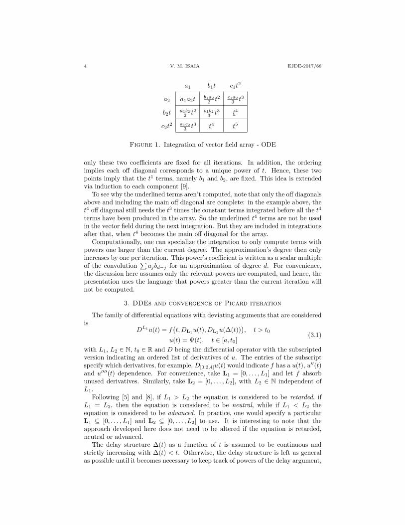
For example, the array in Figure 2 would represent the case of a vector fieldconsisting of a multiplication of two components. A general vector field wouldbe a linear combination of terms, each of which could be represented by such anarray. The linear combination will not disturb what is found in this particularexample. Assume the current approximations are the quadratics a1 + b1t + c1t
2
and a2 + b2t+ c2t2. The empty row and column are included for visual purposes to
accommodate the next power. The underlined terms are not be computed by thisintegration.
To see why powers are invariant with subsequent iteration, note that the constantterms a1 and a2 are fixed by the initial data for all iterations, so all entries involving
4 V. M. ISAIA EJDE-2017/68
a1 b1t c1t2
a2 a1a2tb1a2
2 t2 c1a23 t3
b2ta1b2
2 t2 b1b23 t3 t4
c2t2 a1c2
3 t3 t4 t5
Figure 1. Integration of vector field array - ODE
only these two coefficients are fixed for all iterations. In addition, the orderingimplies each off diagonal corresponds to a unique power of t. Hence, these twopoints imply that the t1 terms, namely b1 and b2, are fixed. This idea is extendedvia induction to each component [9].
To see why the underlined terms aren’t computed, note that only the off diagonalsabove and including the main off diagonal are complete: in the example above, thet4 off diagonal still needs the t3 times the constant terms integrated before all the t4
terms have been produced in the array. So the underlined t4 terms are not be usedin the vector field during the next integration. But they are included in integrationsafter that, when t4 becomes the main off diagonal for the array.
Computationally, one can specialize the integration to only compute terms withpowers one larger than the current degree. The approximation’s degree then onlyincreases by one per iteration. This power’s coefficient is written as a scalar multipleof the convolution
∑ajbd−j for an approximation of degree d. For convenience,
the discussion here assumes only the relevant powers are computed, and hence, thepresentation uses the language that powers greater than the current iteration willnot be computed.
3. DDEs and convergence of Picard iteration
The family of differential equations with deviating arguments that are consideredis
DL1u(t) = f(t,DL1u(t), DL2u(∆(t))
), t > t0
u(t) = Ψ(t), t ∈ [a, t0](3.1)
with L1, L2 ∈ N, t0 ∈ R and D being the differential operator with the subscriptedversion indicating an ordered list of derivatives of u. The entries of the subscriptspecify which derivatives, for example, D[0,2,4]u(t) would indicate f has a u(t), u′′(t)and u′′′′(t) dependence. For convenience, take L1 = [0, . . . , L1] and let f absorbunused derivatives. Similarly, take L2 = [0, . . . , L2], with L2 ∈ N independent ofL1.
Following [5] and [8], if L1 > L2 the equation is considered to be retarded, ifL1 = L2, then the equation is considered to be neutral, while if L1 < L2 theequation is considered to be advanced. In practice, one would specify a particularL1 ⊆ [0, . . . , L1] and L2 ⊆ [0, . . . , L2] to use. It is interesting to note that theapproach developed here does not need to be altered if the equation is retarded,neutral or advanced.
The delay structure ∆(t) as a function of t is assumed to be continuous andstrictly increasing with ∆(t) < t. Otherwise, the delay structure is left as generalas possible until it becomes necessary to keep track of powers of the delay argument,
EJDE-2017/68 NONLINEAR DIFFERENTIAL EQUATIONS 5
in which case only the linear structure ∆(t) = σt − τ with some 0 < σ ≤ 1 andτ ∈ R+ are addressed.
A state dependent delay structure is also examined, once the role of the delaystructure in the solution is realized, but this will be formal. Only one delay structureis addressed in this article, although an extension of this approach to a singleproblem with several delay structures is possible. In general, the delay structure∆(t) determines the value of a. The specifics of this will appear later in this section.
The initial data needs to be polynomial to adapt PSM to the DDE case. If aproblem has analytic initial data, for example see [2], one could consider approxi-mating via a Taylor polynomial. However, two major proofs here will be relegatedto constant initial data. The difficulties encountered for polynomial initial data arepointed out after the result for the constant case is established. The polynomialinitial data case will be addressed in [7].
The standard change of variables converts (3.1) to a first order system, so thatthe Picard iteration is applied to
Du(t) = f(t,u(t),u(∆(t))
), t > t0
u(t) = Ψ(t), t ∈ [a, t0](3.2)
where 1 ≤ l ≤ maxL ≡ {L1, L2} and u = (ul)Ll=0 is such that ul = Dlu andΨ = (Ψl)Ll=0, hence, Ψl = DlΨ. For constant Ψ, note that DlΨ = 0 for l > 0.Thus, the approximation method to come may also be applied to systems of higherorder DDEs of the form (3.1).
It can be shown that if the method of successive approximations is applied tothis first order system, then the sequence of approximations is uniformly convergentand and its limit solves (3.2) uniquely even if the vector field is not polynomial orautonomous. This proves the existence, uniqueness and continuity of a solution to(3.1). The proof from [4] is now adapted to the deviating argument case, and ageneral, but state independent, delay structure is assumed.
Let f in (3.2) be continuous with respect to t and Lipschitz continuous in theremaining variables on [t0, T ∗]× [−U,U ]2L, with U , T ∗ <∞. Such vector fields arecalled admissible. Denote by Cl1 the Lipschitz constant of admissible f with respectto component ul(t) of u(t) and denote by Cl2 the Lipschitz constant of admissible fwith respect to component ul(t) of u(∆(t)). Define Cf ≡
∑Ll=0 C
l1 +Cl2 and Mf ≡
maxl max[t0,T∗] f . General initial data is assumed in the following proposition.
Proposition 3.1. For admissible vector fields f , let T ≡ min{T ∗, UM−1f } and let
Ψ in (3.2) be analytic and such that maxl max[a,T∗] |Ψ(t) − Ψ(t0)| < ∞ and fort > t0, let u0(t) = Ψ(t). For each k ≥ 0 define
uk+1(t) = uk(τ0) +∫ t
t0
f(s,uk(s),uk(∆(s))
)ds (3.3)
then uk(t) converges uniformly to some u∗(t), which solves (3.2) uniquely over[t0, T ].
Proof. Analyticity of Ψ implies u0 ∈ C1([t0, T ]). Applying induction, let uk ∈C1([t0, T ]). Since each component of f is continuous, the Fundamental Theorem ofCalculus implies uk+1 ∈ C1([t0, T ]), so uk ∈ C1([t0, T ]) for k ∈ Z+.
Denote ulk as a component of uk(t) and denote Ψl and f l as components of Ψ andf , respectively. Denote f lk(t) = f l(t,uk(t),uk(∆(t)). One has for every 1 ≤ l ≤ L
6 V. M. ISAIA EJDE-2017/68
that
|ul1 − ul0|(t) =∣∣Ψl(t0) +
∫ t
t0
f l0(s) ds−Ψl(t)∣∣ ≤MΨ +Mf (t− t0)
which follows since |Ψl(t) − Ψl(t0)| ≤ MΨ ≡ maxl max[a,T ] |Ψ(t) −Ψ(t0)| < ∞ byhypothesis.
Consider |ul1 − ul0|(∆(t)). If ∆(t) ≤ t0, then
|ul1 − ul0|(∆(t)) = |Ψl(∆(t))−Ψl(∆(t))| = 0
otherwise, if ∆(t) > t0, then
|ul1 − ul0|(∆(t)) ≤∣∣Ψl(t0) +
∫ ∆(t)
t0
f l0(s) ds−Ψl(∆(t))∣∣ ≤MΨ +Mf (t− t0)
since ∆(t) < t by hypothesis. So both |ul1 − ul0|(t) and |ul1 − ul0|(∆(t)) are boundby MΨ +Mf (t− t0) for every 1 ≤ l ≤ L.
From the Lipschitz continuity of f and the previous bound, one has
|ul2 − ul1|(t) ≤∫ t
t0
|f l1 − f l0|(s) ds ≤∫ t
t0
Cf(MΨ +Mf (s− t0)
)ds (3.4)
so |ul2 − ul1|(t) ≤ Cf(
12Mf (t− t0)2 +MΨ(t− t0)
)for every 1 ≤ l ≤ L. Moving to
the delayed terms, if ∆(t) < t0 then |ul2 − ul1|(∆(t)) = 0 as before, otherwise
|ul2 − ul1|(∆(t)) ≤∫ ∆(t)
t0
|f l1 − f l0|(s) ds ≤∫ t
t0
|f l1 − f l0|(s) ds
and so |ul2−ul1|(∆(t)) along with |ul2−ul1|(t) are both bound by Cf(
12Mf (t− t0)2 +
MΨ(t− t0)). Continuing in this fashion shows that
|ulk+1 − ulk|(t) ≤∫ t
t0
|f lk − f lk−1|(s) ds
≤∫ t
t0
Ckf
(MΨ
(t− t0)k−1
k − 1!+Mf
(t− t0)k
k!
)ds
(3.5)
subsequently, one has
|ulk+1 − ulk|(t) ≤ Ckf(MΨ
(t− t0)k
k!+Mf
(t− t0)k+1
k + 1!
)which implies that for every component 1 ≤ l ≤ L,
∞∑k=0
|ulk+1 − ulk|(t) ≤ (MΨ +Mf (t− t0))∞∑k=0
Ckf(t− t0)k
k!
and one can conclude that for each component ulk,
ulk+1 =∑k
ulk+1 − ulk ≤ (MΨ +Mf (t− t0)) eCf (t−t0)
and so ulk → ul∗ uniformly by Weierstrass M-test with ul∗ continuous. Hence (3.3)holds in the limit, which is equivalent to u∗ = (ul∗)
Ll=1 solving (3.2) since the uniform
convergence allows the limit to be exchanged with the integral. Using the boundsdeveloped above and adapting the argument from [8], it is straightforward to showthat u∗ is unique. �
EJDE-2017/68 NONLINEAR DIFFERENTIAL EQUATIONS 7
The method of successive approximation is a global approximation, in that itupdates uk over [τ0, T ]. However, such a global update is computationally difficultwith a DDE. On the other hand, the method of steps, see [1] for example, iscomputationally friendly but at the expense of being a local approximation. Forthe method of steps, the approach is to reduce (3.1) to a sequence of ODEs: givent0, then prior to a certain point in time, to be determined, terms like u(∆(t)) arefound in terms of Ψ, which is known, so that (3.2) defaults to an ODE, although itmay have non-constant coefficients and/or non-homogeneous terms.
Define τ0 ≡ t0 and denote by τ1 the point in time prior to which u(∆(t)) can befound in terms of Ψ. By standard theory, if the vector field is Lipschitz continuous,then the unique solution that ensues would be valid over [τ0, τ1]. Denote thissolution by u1(t). In order for the delay term u(∆(t)) in the vector field to beknown, ∆(t) must be less than or equal to τ0 over [τ0, τ1]. Using the fact that ∆is strictly increasing and solving ∆(t) = τ0 for t would determine τ1. In addition,∆(τ0) represents the farthest back in time information is needed for the vector field,and so ∆(τ0) = τ−1 = a.
With the problem solved over [τ0, τ1], consider τm defined as the solution to∆(t) = τm−1. Define T ≡ {τm : ∆(τm) = τm−1,m ∈ Z+
0 } and let um(t) be theunique solution to (3.2) over [τm, τm+1]. Consider solving (3.2) over [τm+1, τm+2]to get um+1. Then the delay terms DL2um+1(∆(t)) for t > τm+1 would involveum(t), which is known. Denote the unique solution by um+1(t). Hence
u(t) = {um(t) over [τm, τm+1] for m ∈ Z+} (3.6)
solves (3.2). The overlap in endpoints for the τ -steps is not an issue due to thecontinuity of the solution to (3.2) as per Proposition 3.1.
The method of steps is represented by the intervals [τm, τm+1], or τ -steps, andcomputationally this approach is restrictive in the sense that it updates the solutionone τ -step at a time: the solution needs to be known in [τm−1, τm] before it can bedetermined in [τm, τm+1].
Anticipating the Picard iteration, which will cause the delay structure to becomposed with itself, notice that ∆ : [τm, τm+1]→ [τm−1, τm] satisfies
∆m(t) ≡ ∆ ◦ · · · ◦∆(t) (3.7)
with ∆1(t) = ∆(t) and m > 0. Define ∆0(t) ≡ t = t − τ0 and ∆−1(t) ≡ t − τ−1,where this last definition is for notational convenience. Then ∆m(τm) = 0 for allm ≥ −1. Note that the linear in time and state independent delay
∆(t) = σt+ τ−1 (3.8)
with 0 < σ ≤ 1 and lag τ−1 < 0, includes the constant lag case: ∆(t) = t − τ forsome fixed τ > 0. In this case, one has τm = mτ for all m ≥ 0, while ∆m(t) reducesto t−mτ .
4. dPSM and examples
The PSM philosophy of creating a polynomial environment on which Picard it-eration thrives is now adapted to (3.2). It is important to note that a change ofvariable for the delay terms can come for free, because they may not require anevolution line in the system. Once u(t) evolves, one additional functional evaluationwill give the evolution of u(∆(t)), and taking derivatives will also evolve u′(∆(t)),
8 V. M. ISAIA EJDE-2017/68
u′′(∆(t)) etc. as needed because the Picard iteration explicitly depends on previ-ously computed information. This contributes to making the distinction betweenretarded, neutral and advanced unnecessary as far as implementing this approachis concerned.
Example 4.1. Ignoring the initial information, suppose u′(t) = cos(u(t)) + u(t −τ) + u′(t − τ) with t ≥ t0 6= 0. Following the example in Section 2, introduceV = cos(U) and W = sin(U) along with t = t − t0, u(t) = U(t), R = u(t − τ)and S = u′(t − τ), so that U ′ = V + R + S, V ′ = −WU ′ = −W (V + R + S) andW ′ = V U ′ = V (V +R+ S). Then u′ = cosu+ u(t− τ) + u′(t− τ) is equivalent tothe autonomous polynomial system
x4(t) =
U ′ = V +R+ S
V ′ = −W (V +R+ S)W ′ = V (V +R+ S)
(4.1)
The explicit nature of successive approximations allows the update of R viaR′ = S to be replaced with a function evaluation from U ’s evolution, R(t) =u(t − τ) = U(t − τ). The system may be handled in its current foem, since thevector fields are evaluated at the previous approximation, so only R’s (and S’s)initial information is needed.
There may be a price to pay for the V and W change of variable: if the initialdata is not constant then cos(U) and sin(U) will not be polynomials. This could behandled by using an appropriate Maclaurin polynomial, where the error could pos-sibly be controlled through the choice of the polynomial’s degree. Computationally,there is also a price to pay for non-constant initial data in general.
Parallel to [9], the vector field needs to be autonomous, and evolution needs tobegin at t0 = 0. A change of variable as per the previous example will account forthis, and the explicit t dependence can be dropped from f ’s argument with no otherchange in notation. The variable t, as per the last example, is relabeled as t andthe set T is then determined using this new time variable. Invoking the notationfor the method of steps, the IVP (3.2) becomes, with t0 = τ0 = 0,
u′(t) = f(u(t),u(∆(t))), t > τ0
u(t) = Ψ(t), t ∈ [τ−1, τ0]
where u now includes not only derivatives of u but the auxiliary variables necessaryto make the vector field be polynomial, autonomous and have t0 = 0. Although anordering for the vector is important in practice, there is no reliance on ordering inthe proofs, hence one is not specified.
To compute the Picard iteration over [τ0, T ], the method of steps is used and avery nice computational structure appears once the initial data Ψ is extended overthe entire interval [τ0, T ]. One has
uk+1(t) = uk(τ0) +∫ t
τ0
f(uk(s),uk(∆(s))) ds (4.2)
for t ∈ [τ0, T ] and k ≥ 0. Combining with the method of steps notation, letuk(t) = ukm(t) over [τm, τm+1] with m ∈ Z+
0 . Then (4.2) becomes dPSM, or the
EJDE-2017/68 NONLINEAR DIFFERENTIAL EQUATIONS 9
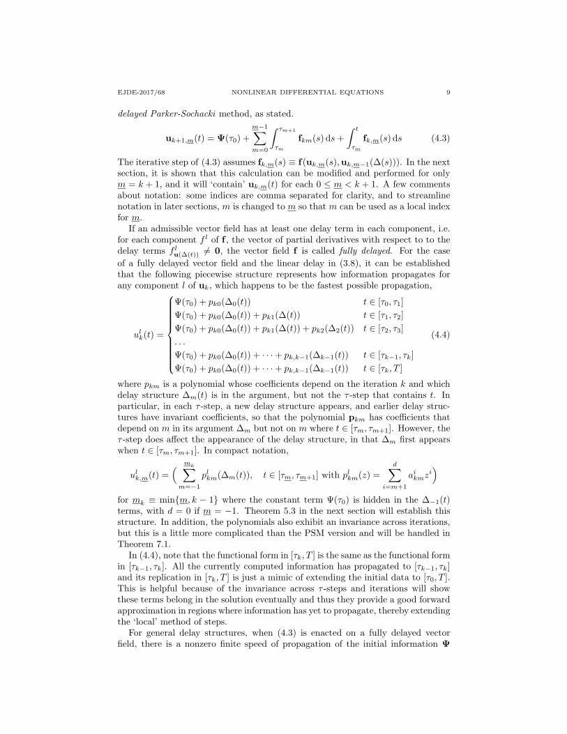
delayed Parker-Sochacki method, as stated.
uk+1,m(t) = Ψ(τ0) +m−1∑m=0
∫ τm+1
τm
fkm(s) ds+∫ t
τm
fk,m(s) ds (4.3)
The iterative step of (4.3) assumes fk,m(s) ≡ f(uk,m(s),uk,m−1(∆(s))). In the nextsection, it is shown that this calculation can be modified and performed for onlym = k + 1, and it will ‘contain’ uk,m(t) for each 0 ≤ m < k + 1. A few commentsabout notation: some indices are comma separated for clarity, and to streamlinenotation in later sections, m is changed to m so that m can be used as a local indexfor m.
If an admissible vector field has at least one delay term in each component, i.e.for each component f l of f , the vector of partial derivatives with respect to to thedelay terms f lu(∆(t)) 6= 0, the vector field f is called fully delayed. For the caseof a fully delayed vector field and the linear delay in (3.8), it can be establishedthat the following piecewise structure represents how information propagates forany component l of uk, which happens to be the fastest possible propagation,
ulk(t) =
Ψ(τ0) + pk0(∆0(t)) t ∈ [τ0, τ1]Ψ(τ0) + pk0(∆0(t)) + pk1(∆(t)) t ∈ [τ1, τ2]Ψ(τ0) + pk0(∆0(t)) + pk1(∆(t)) + pk2(∆2(t)) t ∈ [τ2, τ3]. . .
Ψ(τ0) + pk0(∆0(t)) + · · ·+ pk,k−1(∆k−1(t)) t ∈ [τk−1, τk]Ψ(τ0) + pk0(∆0(t)) + · · ·+ pk,k−1(∆k−1(t)) t ∈ [τk, T ]
(4.4)
where pkm is a polynomial whose coefficients depend on the iteration k and whichdelay structure ∆m(t) is in the argument, but not the τ -step that contains t. Inparticular, in each τ -step, a new delay structure appears, and earlier delay struc-tures have invariant coefficients, so that the polynomial pkm has coefficients thatdepend on m in its argument ∆m but not on m where t ∈ [τm, τm+1]. However, theτ -step does affect the appearance of the delay structure, in that ∆m first appearswhen t ∈ [τm, τm+1]. In compact notation,
ulk,m(t) =( mk∑m=−1
plkm(∆m(t)), t ∈ [τm, τm+1] with plkm(z) =d∑
i=m+1
aikmzi)
for mk ≡ min{m, k − 1} where the constant term Ψ(τ0) is hidden in the ∆−1(t)terms, with d = 0 if m = −1. Theorem 5.3 in the next section will establish thisstructure. In addition, the polynomials also exhibit an invariance across iterations,but this is a little more complicated than the PSM version and will be handled inTheorem 7.1.
In (4.4), note that the functional form in [τk, T ] is the same as the functional formin [τk−1, τk]. All the currently computed information has propagated to [τk−1, τk]and its replication in [τk, T ] is just a mimic of extending the initial data to [τ0, T ].This is helpful because of the invariance across τ -steps and iterations will showthese terms belong in the solution eventually and thus they provide a good forwardapproximation in regions where information has yet to propagate, thereby extendingthe ‘local’ method of steps.
For general delay structures, when (4.3) is enacted on a fully delayed vectorfield, there is a nonzero finite speed of propagation of the initial information Ψ
10 V. M. ISAIA EJDE-2017/68
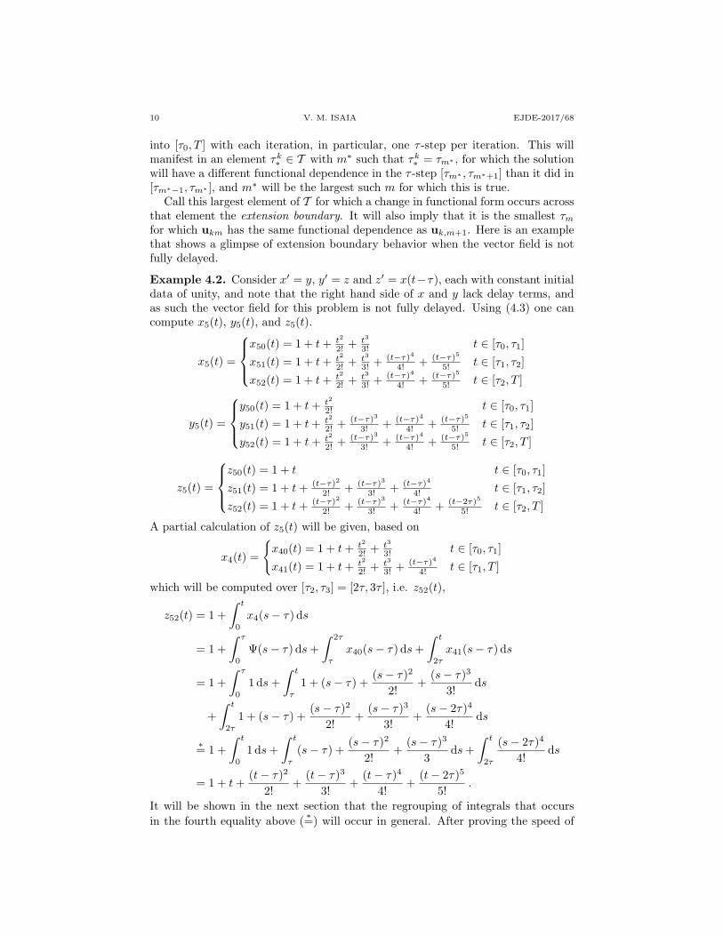
into [τ0, T ] with each iteration, in particular, one τ -step per iteration. This willmanifest in an element τk∗ ∈ T with m∗ such that τk∗ = τm∗ , for which the solutionwill have a different functional dependence in the τ -step [τm∗ , τm∗+1] than it did in[τm∗−1, τm∗ ], and m∗ will be the largest such m for which this is true.
Call this largest element of T for which a change in functional form occurs acrossthat element the extension boundary. It will also imply that it is the smallest τmfor which ukm has the same functional dependence as uk,m+1. Here is an examplethat shows a glimpse of extension boundary behavior when the vector field is notfully delayed.
Example 4.2. Consider x′ = y, y′ = z and z′ = x(t−τ), each with constant initialdata of unity, and note that the right hand side of x and y lack delay terms, andas such the vector field for this problem is not fully delayed. Using (4.3) one cancompute x5(t), y5(t), and z5(t).
x5(t) =
x50(t) = 1 + t+ t2
2! + t3
3! t ∈ [τ0, τ1]
x51(t) = 1 + t+ t2
2! + t3
3! + (t−τ)4
4! + (t−τ)5
5! t ∈ [τ1, τ2]
x52(t) = 1 + t+ t2
2! + t3
3! + (t−τ)4
4! + (t−τ)5
5! t ∈ [τ2, T ]
y5(t) =
y50(t) = 1 + t+ t2
2! t ∈ [τ0, τ1]
y51(t) = 1 + t+ t2
2! + (t−τ)3
3! + (t−τ)4
4! + (t−τ)5
5! t ∈ [τ1, τ2]
y52(t) = 1 + t+ t2
2! + (t−τ)3
3! + (t−τ)4
4! + (t−τ)5
5! t ∈ [τ2, T ]
z5(t) =
z50(t) = 1 + t t ∈ [τ0, τ1]
z51(t) = 1 + t+ (t−τ)2
2! + (t−τ)3
3! + (t−τ)4
4! t ∈ [τ1, τ2]
z52(t) = 1 + t+ (t−τ)2
2! + (t−τ)3
3! + (t−τ)4
4! + (t−2τ)5
5! t ∈ [τ2, T ]
A partial calculation of z5(t) will be given, based on
x4(t) =
{x40(t) = 1 + t+ t2
2! + t3
3! t ∈ [τ0, τ1]
x41(t) = 1 + t+ t2
2! + t3
3! + (t−τ)4
4! t ∈ [τ1, T ]
which will be computed over [τ2, τ3] = [2τ, 3τ ], i.e. z52(t),
z52(t) = 1 +∫ t
0
x4(s− τ) ds
= 1 +∫ τ
0
Ψ(s− τ) ds+∫ 2τ
τ
x40(s− τ) ds+∫ t
2τ
x41(s− τ) ds
= 1 +∫ τ
0
1 ds+∫ t
τ
1 + (s− τ) +(s− τ)2
2!+
(s− τ)3
3!ds
+∫ t
2τ
1 + (s− τ) +(s− τ)2
2!+
(s− τ)3
3!+
(s− 2τ)4
4!ds
∗= 1 +∫ t
0
1 ds+∫ t
τ
(s− τ) +(s− τ)2
2!+
(s− τ)3
3ds+
∫ t
2τ
(s− 2τ)4
4!ds
= 1 + t+(t− τ)2
2!+
(t− τ)3
3!+
(t− τ)4
4!+
(t− 2τ)5
5!.
It will be shown in the next section that the regrouping of integrals that occursin the fourth equality above ( ∗=) will occur in general. After proving the speed of
EJDE-2017/68 NONLINEAR DIFFERENTIAL EQUATIONS 11
the extension boundary with respect to k for a fully delayed vector field, a formaldiscussion of this example’s extension boundary propagation will be given in thenext section.
5. dPSM Results - I
The speed with respect to iterations k will be proved for a general state inde-pendent delay and for a fully delayed vector field. Note that the following result isindependent of the initial data, constant or non-constant.
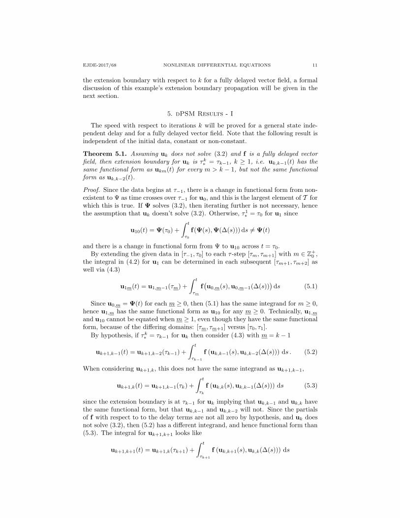
Theorem 5.1. Assuming uk does not solve (3.2) and f is a fully delayed vectorfield, then extension boundary for uk is τk∗ = τk−1, k ≥ 1, i.e. uk,k−1(t) has thesame functional form as ukm(t) for every m > k − 1, but not the same functionalform as uk,k−2(t).
Proof. Since the data begins at τ−1, there is a change in functional form from non-existent to Ψ as time crosses over τ−1 for u0, and this is the largest element of T forwhich this is true. If Ψ solves (3.2), then iterating further is not necessary, hencethe assumption that uk doesn’t solve (3.2). Otherwise, τ1
∗ = τ0 for u1 since
u10(t) = Ψ(τ0) +∫ t
τ0
f(Ψ(s),Ψ(∆(s))) ds 6= Ψ(t)
and there is a change in functional form from Ψ to u10 across t = τ0.By extending the given data in [τ−1, τ0] to each τ -step [τm, τm+1] with m ∈ Z+
0 ,the integral in (4.2) for u1 can be determined in each subsequent [τm+1, τm+2] aswell via (4.3)
u1m(t) = u1,m−1(τm) +∫ t
τm
f(u0,m(s),u0,m−1(∆(s))
)ds (5.1)
Since u0,m = Ψ(t) for each m ≥ 0, then (5.1) has the same integrand for m ≥ 0,hence u1,m has the same functional form as u10 for any m ≥ 0. Technically, u1,m
and u10 cannot be equated when m ≥ 1, even though they have the same functionalform, because of the differing domains: [τm, τm+1] versus [τ0, τ1].
By hypothesis, if τk∗ = τk−1 for uk then consider (4.3) with m = k − 1
uk+1,k−1(t) = uk+1,k−2(τk−1) +∫ t
τk−1
f (uk,k−1(s),uk,k−2(∆(s))) ds . (5.2)
When considering uk+1,k, this does not have the same integrand as uk+1,k−1,
uk+1,k(t) = uk+1,k−1(τk) +∫ t
τk
f (uk,k(s),uk,k−1(∆(s))) ds (5.3)
since the extension boundary is at τk−1 for uk implying that uk,k−1 and uk,k havethe same functional form, but that uk,k−1 and uk,k−2 will not. Since the partialsof f with respect to to the delay terms are not all zero by hypothesis, and uk doesnot solve (3.2), then (5.2) has a different integrand, and hence functional form than(5.3). The integral for uk+1,k+1 looks like
uk+1,k+1(t) = uk+1,k(τk+1) +∫ t
τk+1
f (uk,k+1(s),uk,k(∆(s))) ds
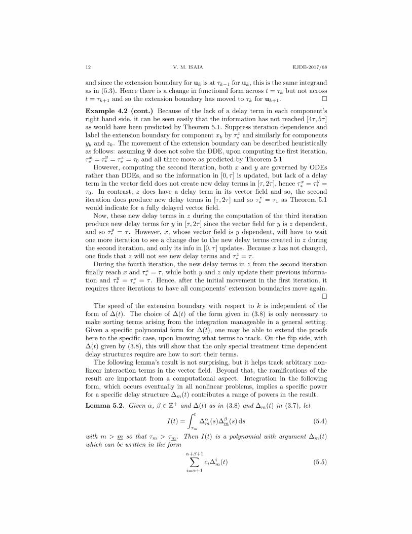
12 V. M. ISAIA EJDE-2017/68
and since the extension boundary for uk is at τk−1 for uk, this is the same integrandas in (5.3). Hence there is a change in functional form across t = τk but not acrosst = τk+1 and so the extension boundary has moved to τk for uk+1. �
Example 4.2 (cont.) Because of the lack of a delay term in each component’sright hand side, it can be seen easily that the information has not reached [4τ, 5τ ]as would have been predicted by Theorem 5.1. Suppress iteration dependence andlabel the extension boundary for component xk by τx∗ and similarly for componentsyk and zk. The movement of the extension boundary can be described heuristicallyas follows: assuming Ψ does not solve the DDE, upon computing the first iteration,τx∗ = τy∗ = τz∗ = τ0 and all three move as predicted by Theorem 5.1.
However, computing the second iteration, both x and y are governed by ODEsrather than DDEs, and so the information in [0, τ ] is updated, but lack of a delayterm in the vector field does not create new delay terms in [τ, 2τ ], hence τx∗ = τy∗ =τ0. In contrast, z does have a delay term in its vector field and so, the seconditeration does produce new delay terms in [τ, 2τ ] and so τz∗ = τ1 as Theorem 5.1would indicate for a fully delayed vector field.
Now, these new delay terms in z during the computation of the third iterationproduce new delay terms for y in [τ, 2τ ] since the vector field for y is z dependent,and so τy∗ = τ . However, x, whose vector field is y dependent, will have to waitone more iteration to see a change due to the new delay terms created in z duringthe second iteration, and only its info in [0, τ ] updates. Because x has not changed,one finds that z will not see new delay terms and τz∗ = τ .
During the fourth iteration, the new delay terms in z from the second iterationfinally reach x and τx∗ = τ , while both y and z only update their previous informa-tion and τy∗ = τz∗ = τ . Hence, after the initial movement in the first iteration, itrequires three iterations to have all components’ extension boundaries move again.
�
The speed of the extension boundary with respect to k is independent of theform of ∆(t). The choice of ∆(t) of the form given in (3.8) is only necessary tomake sorting terms arising from the integration manageable in a general setting.Given a specific polynomial form for ∆(t), one may be able to extend the proofshere to the specific case, upon knowing what terms to track. On the flip side, with∆(t) given by (3.8), this will show that the only special treatment time dependentdelay structures require are how to sort their terms.
The following lemma’s result is not surprising, but it helps track arbitrary non-linear interaction terms in the vector field. Beyond that, the ramifications of theresult are important from a computational aspect. Integration in the followingform, which occurs eventually in all nonlinear problems, implies a specific powerfor a specific delay structure ∆m(t) contributes a range of powers in the result.
Lemma 5.2. Given α, β ∈ Z+ and ∆(t) as in (3.8) and ∆m(t) in (3.7), let
I(t) =∫ t
τm
∆αm(s)∆β
m(s) ds (5.4)
with m > m so that τm > τm. Then I(t) is a polynomial with argument ∆m(t)which can be written in the form
α+β+1∑i=α+1
ci∆im(t) (5.5)
EJDE-2017/68 NONLINEAR DIFFERENTIAL EQUATIONS 13
with ci constant with respect to t.
Proof. Let τ ≡ −τ−1 and some straightforward computation shows that τm =τ∑mq=1 σ
−q and ∆m(t) = σm(t − τm). Rather than Taylor expand the integrand,consider the substitution given by S = ∆m(s), dS = σm ds in (5.4). Rewriting
τm − τm = τ
m∑q=m+1
σ−q ≡ γm,mτ
and using the binomial expansion on (σm−mS + σmγm,mτ)β , we have
I(t) = (σβ(m−m)−m)β∑i=0
(β
i
)(γm,mτ)β−i
i+ α+ 1(σm(t− τm))i+α+1
and note that the powers of τ are independent of α. Upon shifting the index, letting
ci = (σβ(m−m)−m)α+β+1∑i=α+1
(β
i− α− 1
)(γm,mτ)α+β+1−i
i
and exchanging σm(t− τm) with ∆m(t), one recovers (5.5). �
For the constant lag case, ∆m(t) = t − mτ and γm,m = m − m. Nonlinearinteraction in the vector field will cause (5.4) and so the coefficients in the powerseries for the approximation will be lag dependent. These lag dependent coefficientswill also occur when the initial data in (3.2) is not constant.
The next theorem will show that there is a particular structure to the Picarditerations with respect to the τ -steps during a fixed iteration. This is simpler todemonstrate than the structure with respect to iterations k.
Theorem 5.3. If u0,m(t) = Ψ, i.e. constant initial data, for m ∈ Z with m ≥ −1,then define uk,m(t) by (4.3) for k ≥ 1 with ∆(t) as in (3.8). If t ∈ [τm, τm+1] ⊂[τ0, T ], f is fully delayed and defining a0
k,−1 ≡ Ψ(τ0), then uk,m(t) has the form fork ≥ 0
uk,m(t) =mk∑
m=−1
pkm(t) (5.6)
where mk ≡ min{m, k − 1} and ∆0(t) = t− τ0 and ∆−1(t) = t− τ−1. In addition,pkm is a polynomial of the form
pkm(t) =d∑
i=m+1
aikm∆im(t) (5.7)
with d ∈ Z+, d ≥ k if m ≥ 0, d = 0 if m = −1, and the domain of pkm is [τm, T ].
An important point is that the only m dependence in uk,m occurs from mk.
Proof of Theorem 5.3. Clearly, starting with polynomial (constant) initial data andenacting (4.3) implies uk is polynomial for any polynomial vector field and anyk ≥ 0. Hence the focus is on the specific forms of the polynomials in (5.6) given by(5.7).
If the the initial data Ψ is constant, then (5.1) yields for all m ≥ 0
u1m(t) = Ψ(τ0) + z(t− τ0) = Ψ(τ0) + p10(t)
14 V. M. ISAIA EJDE-2017/68
with a110 = z for every [τm, τm+1], where z = f(Ψ,Ψ) is constant since Ψ constant.
It follows that both (5.6) and (5.7) hold with d = 1 when m ≥ 0 and d = 0 whenm = −1 for each τ -step of u1(t).
Some convenient notation will now be introduced. Since f is polynomial, its fullTaylor series is a finite sum with respect to any center. Denote the Taylor series forf(a+ c, b+ d) without its constant term by f∗(a, b; c, d), which represents a powerseries of the form
f∗(a, b; c, d) ≡n∑
(i,j) 6=
n∑(0,0)
Cij(a, b)cidj
for some set of constants Cij which depend on a and b. In addition, we denote
fk,m(s) ≡ f(uk,m(s),uk,m−1(∆(s))
)as well as
f∗k,m−1(s) ≡ f∗(u∗k,m−1(s),u∗k,m−2(∆(s)); pk,m(s),pk,m−1(∆(s))
)Using (5.6) and (5.7) as hypothesis for uk, consider uk+1 during any τ -step [τm, τm+1]with m ≤ k − 1, so that (4.3) implies
uk+1,m(t) = Ψ(τ0) +m−1∑m=0
∫ τm+1
τm
fkm(s) ds+∫ t
τm
fk,m(s) ds
and after a Taylor expansion around the point(uk,m−1(s),uk,m−2(∆(s))
), we have
uk+1,m(t) = Ψ(τ0) +m−1∑m=0
∫ τm+1
τm
fkm(s) ds+∫ t
τm
fk,m−1(s) + f∗k,m−1(s) ds
≡ Iσ(t) + Im(t)
Note that the first term in the integrand of Im(t) has precisely the same functionalform as the m = m − 1 term in the integrand of Iσ(t), so these integrals may becombined to run over [τm−1, t] with t > τm. This demonstrates that the solutioninherits the previous τ -step’s functional form in the next τ -step, [τm, τm+1], whichincludes delay structures from ∆0(t) up to ∆m−1(t).
Using Lemma 5.2 on the integration of f∗k,m−1, which has arguments of ∆m(t)and ∆m−1(∆(t)) = ∆m(t) respectively, which implies (5.6) holds by induction.When m = k, this also introduces a new delay structure given by ∆k(t). In partic-ular, this new delay structure’s minimum power is the minimum power on ∆k−1(t)in pk,k−1 plus one. Then (5.7) holds for the new delay terms m = k, so that (5.7)holds for all k by induction. �
If the initial data is not constant, then it is possible that the constant termassociated with the vector field terms may change across τ -steps. Hence, becausethere is no initial invariance across τ -steps in the constant term, there can be noinvariance with respect to τ in general for any coefficients. This does not precludeusing dPSM, it just makes it ‘trickier’.
6. Iteration structure - formal
6.1. Basic array setup. For DDEs, the PSM invariance result with respect toiterations is true if the vector field is linear, however, it requires a modification forthe nonlinear case, because of the interaction between different delay structures.
EJDE-2017/68 NONLINEAR DIFFERENTIAL EQUATIONS 15
In particular, lower order terms will have their coefficients changed during eachiteration. But upon considering these coefficients as functions of τ , it will be thatthe coefficients on τs for fixed s ≤ k are invariant as k increases. In addition,tracking powers of ∆m(t), one can ascertain whether all terms of a given power arecomputed or not by the integration.
To aid in the proof for the deviating argument case, it is convenient to note thata polynomial vector field associated with (3.2) can be reduced to a quadratic vectorfield.
Lemma 6.1. If (3.1) is equivalent to (3.2) with f polynomial and solution u, thenthere exists an f such that degree f is two and a component of which solves (3.1).
Proof. See [3], noting that deviating arguments may be relabeled in a similar fashionas non-deviating arguments and a change of variable for the deviating argumentsmay not contribute to the size of the vector field since an evolution line may notbe required. �
This result is not necessary but invoking its result streamlines the upcomingproof of the structure between iterations by only having to consider sums of singlemultiplications in the vector field. Each multiplication can be represented by anarray with monomials from the current approximations representing a row or col-umn. The entries of the array would then represent the integration of the row andcolumn monomial multiplication.
Example 6.2. Let y′ = (y(t − τ))r for constant τ with t0 = 0. The vector fieldis not polynomial unless r ∈ Z+, so assume otherwise. To recast the vector fieldfor dPSM, let u = (y(t − τ))r which implies that u′ = r(y(t − τ))r−1y′(t − τ) =ru(y(t − τ))−1y′(t − τ). Note that the derivative term can be computed duringPicard’s iteration from the current approximation for y (after delaying it and takinga derivative), hence it does not require its own evolution line. This can be rewrittenin terms of letters already in use by noting that (y(t−τ))′ = y′(t−τ) = (y(t−2τ))r =u(t−τ) ≡ u∗ upon using the DDE. The u′ line can now be updated to u′ = ruu∗y
−1∗ ,
where the asterisk will denote in general delaying the current argument by τ .The y−1
∗ term needs to be in polynomial form still, so to this end, let v = y−1∗ ,
so that v′ = −1y−2∗ y′∗ = −v2y′∗ = −v2u∗ and the u′ line becomes polynomial as
well. With these change of variables in place, the original DDE can be written asa two component system
u′ = ruvu∗
v′ = −v2u∗(6.1)
and then integrating u will recover the original variable y. However, this system iscubic. A quadratic one can be made to appear, at the price of moving to a threecomponent system, with the addition of w = vu∗ which implies w′ = −w2 + vu′∗.this updates (6.1) to the following system
u′ = ruw
v′ = −vww′ = −w2 + vu′∗
(6.2)
which is quadratic. Note that if one were to compute by hand, (6.1) is preferableto (6.2), but for the proofs, (6.2) is preferred.
16 V. M. ISAIA EJDE-2017/68
Using Theorem 5.3, let uk,m(t) =∑mm=0 pkm(t). It is convenient to arrange
each component of uk as an ordered list rather than an array across i and m.To this end, given ulk, suppress the component dependence, and consider Ul
k =[Pk0(t), . . . , Pk,k−1(t)] where Pk,m(t) = [∆m(t), . . . ,∆d
m(t)], where coefficient infor-mation will be suppressed, to focus on tracking powers of ∆m(t).
Because there will be two components to track in the multiplications of a qua-dratic vector field, the indices m and m will now be used as independent indicestracking the delay structures. Let ul1k generate Ul1
k = (Pkm)i and ul2k generateUl2k = (Qk,m)j , an array may be used to represent the quadratic terms, which can
be thought of in block form Ul1k Ul2
k = (Pkm)i(Qk,m)j . In each entry of the array,tabulate the integration of the corresponding terms (Pkm)i(Qk,m)j by listing theresult in the form ∆i
m(t). The entries of these arrays would then be scalar multi-plied and summed over components to achieve the integration of the entire vectorfield.
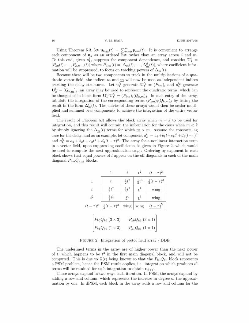
The result of Theorem 5.3 allows the block array when m = k to be used forintegration, and this result will contain the information for the cases when m < kby simply ignoring the ∆m(t) terms for which m > m. Assume the constant lagcase for the delay, and as an example, let component ul1k = a1+b1t+c1t2+d1(t−τ)2
and ul2k = a2 + b2t + c2t2 + d2(t − τ)2. The array for a nonlinear interaction term
in a vector field, upon suppressing coefficients, is given in Figure 2, which wouldbe used to compute the next approximation uk+1. Ordering by exponent in eachblock shows that equal powers of t appear on the off diagonals in each of the maindiagonal PkmQk,m blocks.
1 t t2 (t− τ)2
1 t 12 t
2 13 t
3 13 (t− τ)3
t 12 t
2 13 t
3 t4 wing
t2 13 t
3 t4 t5 wing
(t− τ)2 13 (t− τ)3 wing wing (t− τ)5
Pk0Qk0 (3× 3) Pk0Qk1 (3× 1)
Pk1Qk0 (1× 3) Pk1Qk1 (1× 1)
Figure 2. Integration of vector field array - DDE
The underlined terms in the array are of higher power than the next powerof t, which happens to be t3 in the first main diagonal block, and will not becomputed. This is due to Ψ(t) being known so that the Pk0Qk0 block representsa PSM problem, hence the PSM result applies, i.e. integration which produces tk
terms will be retained for uk’s integration to obtain uk+1.These arrays expand in two ways each iteration. In PSM, the arrays expand by
adding a row and column, which represents the increase in degree of the approxi-mation by one. In dPSM, each block in the array adds a row and column for the
EJDE-2017/68 NONLINEAR DIFFERENTIAL EQUATIONS 17
same reason, while overall the array also adds a new block row and block column,which corresponds to the newest delay term ∆k(t).
6.2. Wing terms. Associated with each main diagonal block PkmQkm with m 6= 0fixed, are off diagonal blocks, PkmQk,m and Pk,mQ
km with 0 ≤ m < m. Ignoringthe constant term multiplications, the remaining terms, referred to as wing terms,are a complication since Lemma 5.2 implies that an integration will produce termswith the same delay as the main diagonal block m, hence their contribution has tofactor into when terms should be computed.
In particular, because of the range of powers produced by Lemma 5.2, wing termsallow the coefficients on lower powers of ∆m(t) to change after each iteration, whichis contrary to the PSM result. However, this coefficient change is predictable and itoccurs through the development of a lag dependence in the coefficients, which willbe polynomial with argument γm,mτ = τ
∑mr=m σ
−r, for the delay structure givenby (3.8) with τ−1 relabeled as τ . Looking at just the coefficients, then a version ofthe PSM result holds, where the only change in coefficients in the next iteration isthe inclusion of the next power of τ .
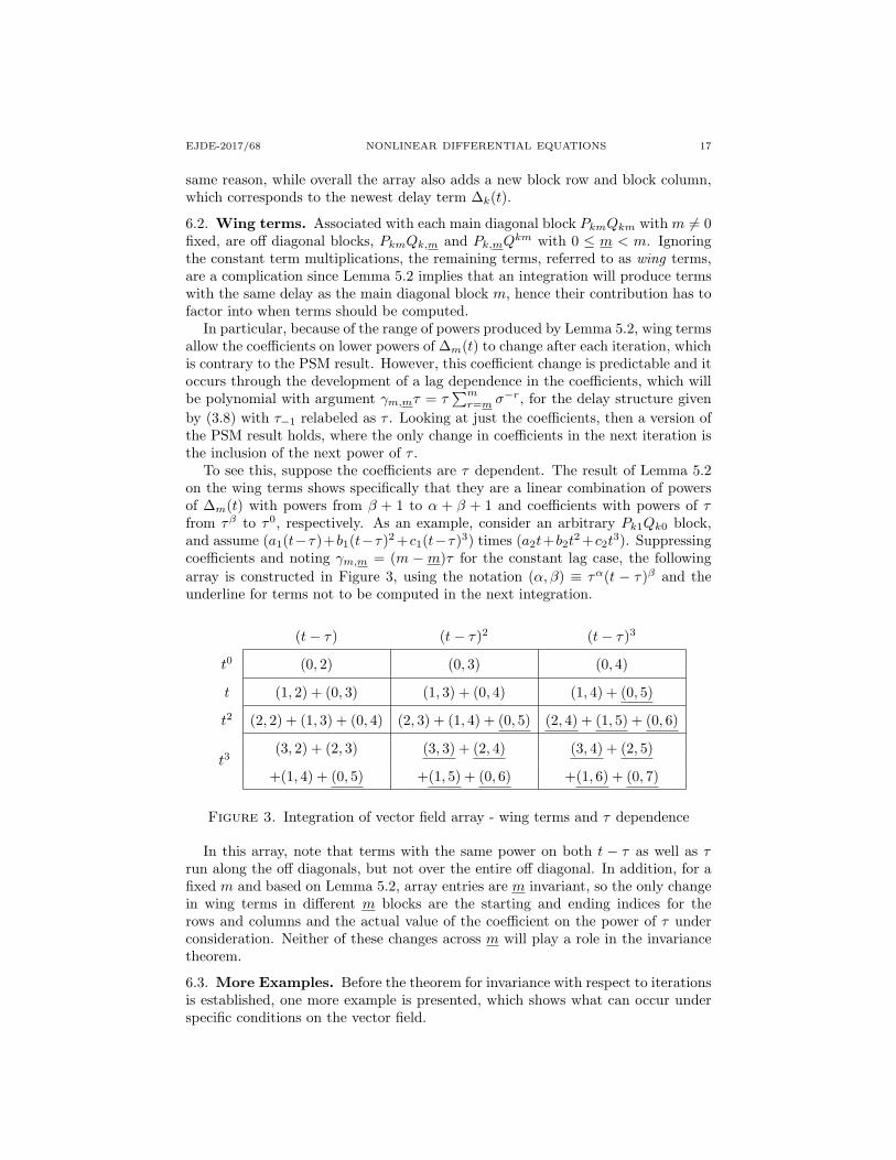
To see this, suppose the coefficients are τ dependent. The result of Lemma 5.2on the wing terms shows specifically that they are a linear combination of powersof ∆m(t) with powers from β + 1 to α + β + 1 and coefficients with powers of τfrom τβ to τ0, respectively. As an example, consider an arbitrary Pk1Qk0 block,and assume (a1(t−τ)+b1(t−τ)2 +c1(t−τ)3) times (a2t+b2t
2 +c2t3). Suppressing
coefficients and noting γm,m = (m −m)τ for the constant lag case, the followingarray is constructed in Figure 3, using the notation (α, β) ≡ τα(t − τ)β and theunderline for terms not to be computed in the next integration.
(t− τ) (t− τ)2 (t− τ)3
t0 (0, 2) (0, 3) (0, 4)
t (1, 2) + (0, 3) (1, 3) + (0, 4) (1, 4) + (0, 5)
t2 (2, 2) + (1, 3) + (0, 4) (2, 3) + (1, 4) + (0, 5) (2, 4) + (1, 5) + (0, 6)
t3(3, 2) + (2, 3) (3, 3) + (2, 4) (3, 4) + (2, 5)
+(1, 4) + (0, 5) +(1, 5) + (0, 6) +(1, 6) + (0, 7)
Figure 3. Integration of vector field array - wing terms and τ dependence
In this array, note that terms with the same power on both t − τ as well as τrun along the off diagonals, but not over the entire off diagonal. In addition, for afixed m and based on Lemma 5.2, array entries are m invariant, so the only changein wing terms in different m blocks are the starting and ending indices for therows and columns and the actual value of the coefficient on the power of τ underconsideration. Neither of these changes across m will play a role in the invariancetheorem.
6.3. More Examples. Before the theorem for invariance with respect to iterationsis established, one more example is presented, which shows what can occur underspecific conditions on the vector field.
18 V. M. ISAIA EJDE-2017/68
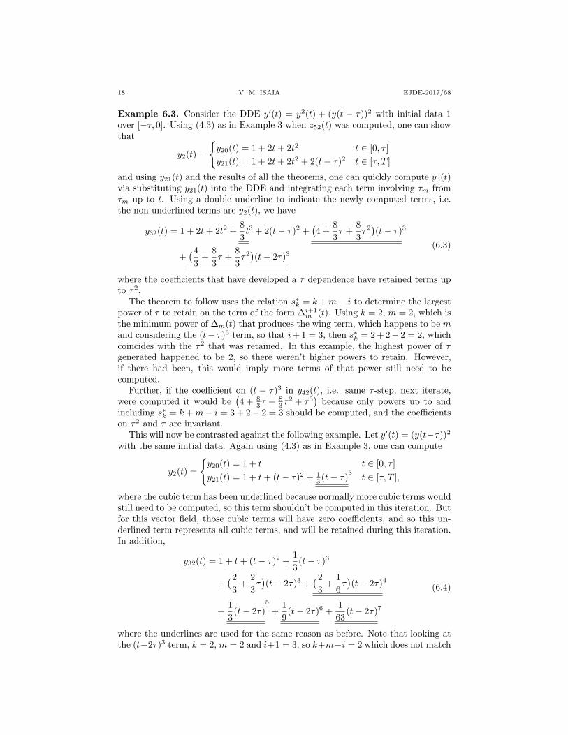
Example 6.3. Consider the DDE y′(t) = y2(t) + (y(t − τ))2 with initial data 1over [−τ, 0]. Using (4.3) as in Example 3 when z52(t) was computed, one can showthat
y2(t) =
{y20(t) = 1 + 2t+ 2t2 t ∈ [0, τ ]y21(t) = 1 + 2t+ 2t2 + 2(t− τ)2 t ∈ [τ, T ]
and using y21(t) and the results of all the theorems, one can quickly compute y3(t)via substituting y21(t) into the DDE and integrating each term involving τm fromτm up to t. Using a double underline to indicate the newly computed terms, i.e.the non-underlined terms are y2(t), we have
y32(t) = 1 + 2t+ 2t2 +83t3 + 2(t− τ)2 +
(4 +
83τ +
83τ2)(t− τ)3
+(4
3+
83τ +
83τ2)(t− 2τ)3
(6.3)
where the coefficients that have developed a τ dependence have retained terms upto τ2.
The theorem to follow uses the relation s∗k = k +m− i to determine the largestpower of τ to retain on the term of the form ∆i+1
m (t). Using k = 2, m = 2, which isthe minimum power of ∆m(t) that produces the wing term, which happens to be mand considering the (t− τ)3 term, so that i+ 1 = 3, then s∗k = 2 + 2− 2 = 2, whichcoincides with the τ2 that was retained. In this example, the highest power of τgenerated happened to be 2, so there weren’t higher powers to retain. However,if there had been, this would imply more terms of that power still need to becomputed.
Further, if the coefficient on (t − τ)3 in y42(t), i.e. same τ -step, next iterate,were computed it would be
(4 + 8
3τ + 83τ
2 + τ3)
because only powers up to andincluding s∗k = k +m− i = 3 + 2− 2 = 3 should be computed, and the coefficientson τ2 and τ are invariant.
This will now be contrasted against the following example. Let y′(t) = (y(t−τ))2
with the same initial data. Again using (4.3) as in Example 3, one can compute
y2(t) =
{y20(t) = 1 + t t ∈ [0, τ ]y21(t) = 1 + t+ (t− τ)2 + 1
3 (t− τ)3t ∈ [τ, T ],
where the cubic term has been underlined because normally more cubic terms wouldstill need to be computed, so this term shouldn’t be computed in this iteration. Butfor this vector field, those cubic terms will have zero coefficients, and so this un-derlined term represents all cubic terms, and will be retained during this iteration.In addition,
y32(t) = 1 + t+ (t− τ)2 +13
(t− τ)3
+(2
3+
23τ)(t− 2τ)3 +
(23
+16τ)(t− 2τ)4
+13
(t− 2τ)5
+19
(t− 2τ)6 +163
(t− 2τ)7
(6.4)
where the underlines are used for the same reason as before. Note that looking atthe (t−2τ)3 term, k = 2, m = 2 and i+1 = 3, so k+m−i = 2 which does not match
EJDE-2017/68 NONLINEAR DIFFERENTIAL EQUATIONS 19
the term τ1. Here, constant initial data and the lack of t arguments in the vectorfield produce only t − τ terms, and none of higher power. Hence the assumptionsthat went into forming k+m− i above need to be revisited, in particular, k shouldbe replaced by k − 1 here.
7. dPSM results - II
The next theorem is essentially the invariance of coefficients idea from Theorem4.1 but with respect to k rather than with respect to m with consideration of a τdependence. The theorem holds if Ψ is not constant, but in light of Theorem 5.3,only in a fixed τ -step.
The fastest propagation occurs when the vector fields have an additional con-dition placed on them. A mixing vector field is fully delayed and has in eachcomponent, either a term of the form u(t)v(∆(t)), otherwise terms of the formu(t)v(t) +w(∆(t))x(∆(t)), where u, v, w and x are any components, some or all ofwhich may be the same. Note that the first vector field in Example 5 falls into thiscategory, while the second one does not.
Theorem 7.1. Using ∆(t) as in (3.8) and mixing f , then the solution to (3.2) hasthe form (5.6) and (5.7), where the coefficients satisfy
aikm =sk∑s=0
ai,skmτs
for some sk > 0. In addition, for fixed k and fixed i ≤ k and every −1 ≤ m ≤ mk,defined in Theorem 5.3, we have
ai,sk+n,m = ai,skm (7.1)
for each s ≤ s∗ ≡ k +m− i and every n > 0.
Proof. Consider fusing the ordered lists [uk(t),uk(∆(t))] so that the delay terms inthe vector field can be distinguished via the component index: ulk(t) represents the(l − L− 1)th derivative of uk evaluated at ∆(t) if L < l ≤ 2L. Given a solution to(3.2), consider the quadratic vector field for the (k+ 1)th iteration and suppressingtime dependence, we have
Dulk+1 =2L∑l1=1
2L∑l2=1
cll1l2ul1k u
l2k
The indices m and m will now denote independent indices for the delay structurein each component. There is then the need to relabel m, the index for the τ -step,which is now denoted by n. For n < k, (4.3) produces {ulk,n}2Ll1=1, polynomials ofthe form (5.6) and (5.7).
ulk+1,n = ulkn(τ0) +n−1∑m=0
∫ τm+1
τm
2L∑l1=1
2L∑l2=1
cll1l2ul1kmu
l2km ds
+∫ t
τn
cll1l2ul1knu
l2kn ds
(7.2)
Decompose further with
ulkn =nk∑
m=−1
plkm =nk∑
m=−1
( k−1∑i=i∗
ailkm∆im +
d∑i=k
ailkm∆im
)(7.3)
20 V. M. ISAIA EJDE-2017/68
where d is the largest power produced by integrating the vector field and i∗ = n+1if l ≤ L and i∗ = n if l > L. In particular, if n = −1, then d = 0 and both sumscollapse to constant terms. Integrands in (7.2) are a linear combination of functionmultiplications. Substituting (7.3) into (7.2) shows these multiplications each havethe following form:
nk∑m=−1
nk∑m=−1
( k−1∑i=i∗
ail1km∆im
k−1∑i=i∗
ail2k,m∆i
m
)
+nk∑
m=−1
nk∑m=−1
( d∑i=k
ail1km∆im
d∑i=k
ail2k,m∆i
m
)
+nk∑
m=−1
nk∑m=−1
( d∑i=k
ail1km∆im
k−1∑i=i∗
ail2k,m∆i
m
)
+nk∑
m=−1
nk∑m=−1
( k−1∑i=i∗
ail1km∆im
d∑i=k
ail2k,m∆i
m
)≡∑
1
+∑
2
+∑
3
+∑
4
(7.4)
where for simplicity ailkm is taken to be zero if m = 0 and l > L.Intuitively, each individual l1 and l2 will produce a block array of the form
(P l1km)i(P l2k,m)i. In this sense, m and m are indices for the block form of the array,and i and i are local indices inside a particular block.
The multiplication of the sums in the terms of∑
1 demonstrate that the previousiteration’s powers of ∆m(t) contribute to the next iteration. The multiplicationin the terms of
∑2 produces terms with powers of ∆m(t) at least 2k + 1 after
integrating and should not be computed in the next integration since terms ofpower 2k, 2k− 1, . . . , k+ 1 are not yet present in the approximations to contribute.This also applies to powers above k in
∑1.
The multiplications from∑
3 and∑
4 are wing terms, and depending on whetherm > m or m < m, one set will contribute ∆i
m(t) with i ≥ k and will not becomputed, while the other set due to Lemma 5.2, will contribute ∆i
m(t) with i =m + 1, . . . , k. This implies that coefficients for lower powers in general are notinvariant with respect to iterations, however, they can be shown invariant withrespect to iterations when considered as polynomials of τ .
To see this, denote the coefficient on ∆i+1m , with i ≤ k, in the l component of
uk by ai+1,lkm . This coefficient may be a polynomial in τ , and is determined by
summing up the coefficients on all ∆i+1m terms in the arrays for each (l1, l2). Since
i is considered fixed, introduce I, J as independent indices for powers of ∆m. Ineach array, these sums have the form
ai+1,lk+1,m
=2L∑l1=1
2L∑l2=1
[(i+ 1)−1
∑I+J
∑=i
aIl1kmaJl2km
+m−1∑m=−1
( i∑J=m
k∑I=i−J
aIl1k,maJl2kmγτ
IJ +i∑
I=m
k∑J=i−I
aIl1kmaJl2k,mγτ
IJ)] (7.5)
EJDE-2017/68 NONLINEAR DIFFERENTIAL EQUATIONS 21
where γτ IJ ≡ γmmτI+J−i. Note that γm,m is constant with respect to τ and
independent of k. The terms in the first line come out of the appropriate maindiagonal block and the second line has all the wing terms. Note also that theindices have been relabeled so that m is the larger index, while m is the smallerone
Consider now a future integration for the same term ∆i+1m (t) using uk+n,
ai+1,lk+n+1,m =
2L∑l1=1
2L∑l2=1
[(i+ 1)−1
∑I+J
∑=i
aIl1k+n,maJl2k+n,m
+m∑
m=−1
( i∑J=m
k+n∑I=i−J
aIl1k+n,maJl2k+n,mγτ
IJ
+i∑
I=m
k+n∑J=i−I
aIl1k+n,maJl2k+n,mγτ
IJ)]
and upon breaking off the powers above k, we have
ai+1,lk+n+1,m
=2L∑l1=1
2L∑l2=1
[(i+ 1)−1
∑I+J
∑=i
aIl1k+n,maJl2k+n,m
+m∑
m=−1
( i∑J=m
k∑I=i−J
aIl2k+n,maJl2k+n,mγτ
IJ +i∑
I=m
k∑J=i−I
aIl1k+n,maJl2k+n,mγτ
IJ
+i∑
J=m
k+n∑I=k+1
aIl1k+n,maJl2k+n,mγτ
IJ +i∑
I=m
k+n∑J=k+1
aIl1k+n,maJl2k+n,mγτ
IJ)]
(7.6)
For notational convenience, the double sum over l1 and l2 will be suppressed alongwith l1 and l2 dependence, along with denoting aIkm ≡ aIl1km and bJkm ≡ aJl2km. Nowlet k = 0, which implies that m, i and s = 0 in the theorem statement. Theorem(5.3) shows that the theorem statement holds for k = 0.
If the theorem statement holds for arbitrary k, i.e. i ≤ k and s ≤ s∗, then
aIk+n,m = aIkm +d∑
s=s∗+1
aIsk+n,mτs ≡ aIkm + pas∗+1 (7.7)
with a similar statement for bJk+n,m. Inserting (7.7) into (7.6) and expanding, wehave
(i+ 1)−1∑I+J
∑=i
(aIkmb
Jkm + pas∗+1b
Jkm + pbs∗+1a
Ikm + pas∗+1p
bs∗+1
+m−1∑m=−1
( i∑J=m
k∑I=i−J
(aIk,mb
Jkm + pas∗+1b
Jkm + pbs∗+1a
Ik,m + pas∗+1p
bs∗+1
)γτ IJ
+i∑
I=m
k∑J=i−I
(aIkmb
Jk,m + pas∗+1b
Jk,m + pbs∗+1a
Ikm + pas∗+1p
bs∗+1
)γτ IJ
22 V. M. ISAIA EJDE-2017/68
+i∑
J=m
k+n∑I=k+1
(aIk,mb
Jkm + pas∗+1b
Jkm + pbs∗+1a
Ik,m + pas∗+1p
bs∗+1
)γτ IJ
+i∑
I=m
k+n∑J=k+1
(aIkmb
Jk,m + pas∗+1b
Jk,m + pbs∗+1a
Ikm + pas∗+1p
bs∗+1
)γτ IJ
)(7.8)
and note that the first multiplication in the first, second and third lines of (7.8) arethe same terms from (7.5). In the second and third terms in the first line of (7.7),note that a and b may have constant terms. It follows that these terms will havea minimum power of τ given by the minimum power in ps∗+1, which is s∗ + 1 andhence, they may be written in the form P (τ)τs
∗+1 where P is a polynomial witha constant term. All the second and third terms in lines two through five have alarger power of τ than s∗ + 1 and are thus considered higher order. This is alsotrue for all the terms of the form pas∗+1p
bs∗+1.
So, summing over l1 and l2 and explicitly denoting the lowest power of τ in thefirst three lines of (7.8) along with the lowest power of τ in the last two lines, wehave
ai+1k+n+1,m = ai+1
k+1,m + Pτk+m−i +G(τ)
+2L∑l1=1
2L∑l2=1
cll1l2
m−1∑m=m∗
( i∑J=m
k+n∑I=k+1
aIl1k,maJl2kmγτ
IJ
+i∑
I=m
k+n∑J=k+1
aIl1kmaJl2k,mγτ
IJ) (7.9)
where P is a polynomial with respect to τ with a constant term and G(τ) containsthe higher order terms. In addition, both ail1km and ail2km may have constant terms,so that the minimum power of τ in the second line of (7.9) is min I + J − i =k+1+m−i = s∗+1 over both sums. Hence, ai+1,s
k+n+1,m = ai+1,sk+1,m if s ≤ k+m−i−1
and so (5.6) and (5.7) both hold for k + 1, and thus all k. �
Note that both powers of ∆m(t) along with powers of τ from Lemma 5.2 areconstant along off diagonals in each block array. Hence the main diagonal blocksdictate keeping powers of ∆m(t) up to i ≤ k + 1, and then keeping powers of τ upto k +m− i.
PSM also provides an explicit a priori error bound which does not involve deriva-tives of the vector field, [13]. Note that over [τm−1, τm], the structure in Theorem5.3 can be expanded in a series around the single center τm−1. Using this repre-sentation, the error estimate for PSM may be extended to the deviating argumentcase.
Some notation will now be introduced and to facilitate, there is a strong overlapwith the notation in [13]. Denote by ‖v‖∞ = maxl vl, the maximum over thecomponents of v. The vector field will be polynomial and written compactly as
f(u,u∗) =df∑i=0
df∑j=0
Bijuiuj∗
where the sum over the ordered list of indices implies a sum over each index in thelist ranging from 0 to df , the exponentiation between ordered lists is componentwise
EJDE-2017/68 NONLINEAR DIFFERENTIAL EQUATIONS 23
and the asterisk denotes the delay terms. Denote by ‖Bij‖ the maximum row sumof coefficient magnitudes, the subordinate matrix norm to the vector norm ‖ · ‖∞.
If one considers (3.2) globally, then ‖Bij‖ would be the norm of the vector field.There is also occasion to consider the local vector field for the ODE in [τm, τm+1]with the delay info considered ‘known’ and hence, the norm of the vector field wouldneed to incorporate the delay information into the coefficient matrix. Dub the localODE as f∗(u).
Theorem 7.2. For finite m ≥ 0, the expansion ukm(t) =∑mm=−1 pk,m(t) gener-
ated by (4.3) is such that
‖u(t)− ukm(t)‖∞ ≤ Ckm(F (t− τm; ‖Bij‖∞, df )−
k∑q=0
zq(t− τm)q)
(7.10)
when t ∈ [τm, T ] with df + 1 being the vector field’s degree in (3.2) and constantCkm dependent on ‖Ψ‖∞, the norm of the initial data along with
F (t; a, b) = exp(at), b = 0 and F (t; a, b) =1
(1− abt)1/b, b ≥ 1
The sequence elements zq are the expansion coefficients of F which solves z′(t) =azb.
This result holds for non-constant initial data.
Proof. Approximating (3.2) via (4.3), note that in each τ -step, the DDE reduces toan ODE with non-constant coefficients and/or non-homogeneous terms involvingthe solution from the previous τ -step.
To recover an ODE, the vector field must be modified to include the delay in-formation in its coefficients. Summing Biju
j∗ over j would yield coefficients for the
ODE f∗(u) over the particular τ -step. Noting that (3.3) holds in the limit, we have
u∗(t) ≤ max[0,t]
u∗ ≤ max[0,t]
u ≤MΨ + tMf (7.11)
using the notation of Proposition 3.1, and the coefficient matrix satisfies the bound
‖f∗‖ ≤ ‖Bij‖((‖MΨ + τmMf )∗
)df+1 ≡ ‖fm‖
where the asterisk indicates max{·, 1}. Hence, (3.2) becomes the ODE initial valueproblem u′ = f∗(u) with initial data u(τm) = ukm(0), to which the result from [13]can be applied. For convenience, ‖ · ‖∞ is shortened to ‖ · ‖, F (·; ‖fm‖, df + 1) isshortened to Fm(·) and ‖ekm(t)‖ ≡ ‖u(t)− ukm(t)‖. This yields
‖ekm(t)‖ ≤ ‖u∗k,m−1(τm)‖(Fm(t− τm)−
k∑q=0
zqm(t− τm)q)
(7.12)
where the asterisk again indicates max{·, 1} and zqm are the expansion coefficientsof Fm which solves z′(t) = ‖fm‖zdf+1. Using the fact that ‖ekm(t)‖ ≥ 0 along withthe substitution ‖u∗k,m−1(τm)‖ = ‖u(τm)− ek,m−1(τm)‖, we have
‖u∗k,m−1(τm)‖ ≤ max{‖u(τm)‖+ ‖ek,m−1(τm)‖, 1 + ‖ek,m−1(τm)‖}≤ max{‖u(τm)‖, 1}+ ‖ek,−1(τm)‖
24 V. M. ISAIA EJDE-2017/68
Using (3.3) in the limit as before to bound the solution, then (7.12) becomes
‖ekm(t)‖
≤((MΨ + τmMf )∗ + ‖ek,m−1(τm)‖
)(Fm(t− τm)−
k∑q=0
zqm(t− τm)q) (7.13)
and (7.13) may then be continued to
‖ekm(t)‖ ≤ Ckm(Fm(t− τm)−
k∑q=0
zqm(t− τn)q)
which is (7.10), where
Ckm ≡ (MΨ + τmMf )∗m∑m=0
m∏n=m
(Fn(τn+1 − τn)−
k∑q=0
zqn(τn+1 − τn)q)
Note that a slightly less tight, but computationally nicer bound exists for the basicPSM result which could be adapted here, see [13]. �
8. General delay structure
There is a logical difficulty extending Proposition 3.1 to the state dependentdelay case due to the changing nature of ∆ with respect to iterations. Hence, thediscussion of the approximation of this case via dPSM is heuristic. With regardsto (5.6), note that ∆ can only known approximately since u would only be knownapproximately. If one imagines a sequence of approximations ∆k to ∆, these coulddiffer in functional form each iteration, or possibly only in certain parameters, forexample σ and/or τ = τ−1 in the case of (3.8).
If a problem starts in the solution’s basin of attraction so that the basic iterationwould evolve to the correct fixed point, then ∆km(t) = ∆(t,ukm(t)) may be com-puted based on the computation of ukm. At the very least, one needs to store thepolynomial for the τ coefficients so that upon updating the set of τm at each iter-ation based on the currently computed ∆k(t) would allow updating the previouslycomputed coefficients so that they do not have to be recomputed each iteration.In other words, there would be invariance in previously computed coefficients onceτk−1,m is updated to τkm based on ∆km(t).
Acknowledgments. The author would like to thank Drs. James Sochacki andAllen Holder for useful discussions, constructive criticisms and their donations oftime and expertise during the writing of this article.
References
[1] C. T. H. Baker, C. A. H. Paul, D. R. Wille; Issues in the Numerical Solution of EvolutionaryDelay Differential Equations, Adv. Comp. Math, 3 (1995), pp. 171-196.
[2] A. Bellen, N. Guglielmi, A. E. Ruehli; Methods for Linear Systems of Circuit Delay Differen-
tial Equations of Neutral Type, IEEE Transactions on Circuits and Systems - I: FundamentalTheory and Applications, 46 (1999) 1, pp. 212-215.
[3] D. C. Carothers, G. E. Parker, J. S. Sochacki, P. G. Warne; Some Properties of Solutions toPolynomial Systems of Equations, Elec. Jour. of Diff. Eqn., 2005 (2005) 40, pp. 1-17.
[4] E. A. Coddington, N. Levinson; Theory of Ordinary Differential Equations, McGraw-Hill,New York, 1955
[5] L. E. El’sgol’ts; Introduction to the Theory of Differential Equations with Deviating Argu-ments, (translated by R. J. McLaughlin), Holden-Day, San Francisco, 1966
EJDE-2017/68 NONLINEAR DIFFERENTIAL EQUATIONS 25
[6] E. Fehlberg; Numerical Integration of Differential Equations by Power Series Expansions,
Illustrated by Physical Examples, Technical Report NASA-TN-D-2356, NASA, (1964).
[7] V. M. Isaia; dPSM and Polynomial Initial Data, in preparation.[8] S. B. Norkin; Differential Equations of the Second Order with Retarded Argument, Transla-
tions of Mathematical Monographs (L. J. Grimm) vol. 31, AMS, Providence, 1972
[9] G. E. Parker, J. S. Sochacki; Implementing the Picard Iteration, Neural, Parallel and ScientificComputations, 4 (1996) 1, pp. 97-112.
[10] G. E. Parker, J. S. Sochacki; A Picard-Maclaurin Theorem for Initial Value PDEs, Abstr.
Appl. Anal., 5 (2000) 1, pp. 47-63.[11] J. S. Sochacki, A. Tongen; Exploring Polynomial Dynamical Systems: An Interesting Appli-
cation of Power Series to Differential Equations, Springer-Verlag, 2016.
[12] R. D. Stewart, W. Bair; Spiking Neural Network Simulation: Numerical Integration with theParker-Sochacki Method, Journal Computational Neuroscience, 27 (2009), pp. 115-133.
[13] P. G. Warne, D. A. P. Warne, J. S. Sochacki, G. E. Parker, D. C. Carothers; Explicit A-Priori Error Bounds and Adaptive Error Control for Approximation of Nonlinear Initial
Value Differential Systems, Comput. Math. Appl., 52 (2006), pp. 1695-1710.
Vincenzo Michael Isaia
Department of Mathematics, Rose-Hulman Institute of Technology, Terre Haute, IN47803, USA
E-mail address: [email protected]