least-squares solutions of nonlinear differential...
TRANSCRIPT

LEAST-SQUARES SOLUTIONSOF NONLINEAR DIFFERENTIAL EQUATIONS
Daniele Mortari∗, Hunter Johnston†, and Lidia Smith‡
This study shows how to obtain least-squares solutions to initial and boundaryvalue problems of nonlinear differential equations. The proposed method beginsusing an approximate solution obtained by any existing integrator. Then, a least-squares fitting of this approximate solution is obtained using a constrained ex-pression, introduced in Ref. [10]. This expression has embedded the differentialequations constraints. The resulting expression is then used as an initial guess ina Newton iterative process that increases the solution accuracy to machine errorlevel in no more than two iterations for most of the problems considered. For nonsmooth solutions or for long integration times, a piecewise approach is proposed.The highly accurate value estimated at the final time is then used as the new ini-tial guess for the next time range, and this process is repeated for subsequent timeranges. This approach has been validated for the simple oscillator and Duffingoscillator for 10, 000 subsequent time ranges obtaining a 10−12-level of final ac-curacy. A final numerical test is provided for a boundary value problem with aknown solution, requiring 18 iterations to reach machine error accuracy.
Acronyms used throughout this paper
NDE → Nonlinear Differential EquationLDE → Linear Differential EquationIVP → Initial Value ProblemBVP → Boundary Value ProblemMVP →Multi-point Value ProblemLS → Least-Squares
INTRODUCTION
The n-th order nonlinear Differential Equation (DE) is the equation
y(n) = f(y(n−1), y(n−2), · · · , y, y, t
), (1)
where y(k) =dkydtk
, f(·) is a nonlinear function of its arguments, and n ≥ 1. This type of equationappears in many problems and in almost all scientific disciplines.
Equation (1) can be solved by many existing approaches, most of which are based on the Runge-Kutta family of integrators [1]. Other methods include: Gauss-Jackson [2], time domain collocation∗Aerospace Engineering, Texas A&M University, College Station, TX. IEEE and AAS Fellow, AIAA Associate Fellow.E-mail: [email protected]†Aerospace Engineering, Texas A&M University, College Station, TX. E-mail: [email protected]‡Mathematics, Blinn College, College Station, TX. E-mail: [email protected]
1
techniques [3, 4], and Modified Chebyshev-Picard Iteration [5, 6, 7] (a path-length integral approx-imation which has been recently proven to be highly effective). All of these methods are based onlow-order Taylor expansions, which limit the step size that can be used to propagate the solution.
In the Collocation Methods [8] (CM), the solution components are approximated by piecewisepolynomials on a mesh. The coefficients of the polynomials form the unknowns to be computed.The approximation to the solution must satisfy the constraint conditions and the DE at collocationpoints in each mesh subinterval. In the CM the placement of the collocation points is not arbitrary.A modified Newton-type method, known as quasi-linearization, is then used to solve the nonlinearequations for the polynomial coefficients. The mesh is then refined by attempting to equidistributethe estimated error over the whole interval, and therefore an initial estimation of the solution acrossthe mesh is required. A common weakness of all methods based on low-order Taylor expansion isthat they are not effective in enforcing algebraic constraints. This is the actual strength of the pro-posed Least-Squares (LS) method, since the DE constraints are embedded in the searched solutionexpression (constrained expression). This means that all solutions generated by this method per-fectly (meaning analytically) satisfy the DE constraints. The differences between the LS approachand the CM are several. The CM requires the solution satisfying the nonlinear DE in certain points(collocation points) and where the nonlinear DE constraints are defined. The LS uses constrainedexpressions to always satisfy the nonlinear DE constraints. It then looks for the solution as a linearcombination of basis functions. In general, the LS does not satisfy the nonlinear DE at all points, ex-cept for the constraints points. Therefore, while the CM uses piecewise approximation polynomials,LS uses a single analytical expression for the whole range.
Spectral methods [9] are also used to numerically solve DE. In these methods the solution isexpressed as a sum of certain “basis functions” (generally Fourier series) and the coefficients in thesum are computed to satisfy the DE as closely as possible. The boundary conditions must then beenforced, which is done by replacing one (or more) of the equations with the constraints conditions.The proposed method proceeds in the reverse sequence: it first takes care of the constraints byderiving a constrained expression [10] (equation that always satisfies the DE constraints) and thenfinds the least-squares solution by expressing the free function, g(t), of the constrained expressionas a linear combination of “basis functions.”
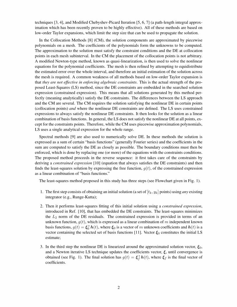
The least-squares method proposed in this study has three steps (see Flowchart given in Fig. 1).
1. The first step consists of obtaining an initial solution (a set of [tk, yk] points) using any existingintegrator (e.g., Runge-Kutta);
2. Then it performs least-squares fitting of this initial solution using a constrained expression,introduced in Ref. [10], that has embedded the DE constraints. The least-squares minimizesthe L2 norm of the DE residuals. The constrained expression is provided in terms of anunknown function, g(t), which is expressed as a linear combination of m independent knownbasis functions, g(t) = ξ T
0 h(t), where ξ0 is a vector of m unknown coefficients and h(t) is avector containing the selected set of basis functions [11]. Vector ξ0 constitutes the initial LSestimate;
3. In the third step the nonlinear DE is linearized around the approximated solution vector, ξ0,and a Newton iterative LS technique updates the coefficients vector, ξ, until convergence isobtained (see Fig. 1). The final solution has g(t) = ξ T
f h(t), where ξf is the final vector ofcoefficients.
2
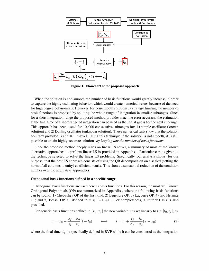
Figure 1. Flowchart of the proposed approach
When the solution is non-smooth the number of basis functions would greatly increase in orderto capture the highly oscillating behavior, which would create numerical issues because of the needfor high degree polynomials. However, for non-smooth solutions, a strategy limiting the number ofbasis functions is proposed by splitting the whole range of integration in smaller subranges. Sincefor a short integration range the proposed method provides machine error accuracy, the estimationat the final time of a short range of integration can be used as the initial guess for the next subrange.This approach has been tested for 10, 000 consecutive subranges for: 1) simple oscillator (knownsolution) and 2) Duffing oscillator (unknown solution). These numerical tests show that the solutionaccuracy provided is at a 10−12-level. Using this technique if the solution is not smooth, it is stillpossible to obtain highly accurate solutions by keeping low the number of basis functions.
Since the proposed method deeply relies on linear LS solver, a summary of most of the knownalternative approaches to perform linear LS is provided in Appendix . Particular care is given tothe technique selected to solve the linear LS problems. Specifically, our analysis shows, for ourpurpose, that the best LS approach consists of using the QR decomposition on a scaled (setting thenorm of all columns to unity) coefficient matrix. This shows a substantial reduction of the conditionnumber over the alternative approaches.
Orthogonal basis functions defined in a specific range
Orthogonal basis functions are used here as basis functions. For this reason, the most well knownOrthogonal Polynomials (OP) are summarized in Appendix , where the following basis functionscan be found: 1) Chebyshev OP of the first kind, 2) Legendre OP, 3) Laguerre OP, 4) two HermiteOP, and 5) Bessel OP, all defined in x ∈ [−1,+1]. For completeness, a Fourier Basis is alsoprovided.
For generic basis functions defined in [x0, xf ] the new variable x is set linearly to t ∈ [t0, tf ], as
x = x0 +xf − x0tf − t0
(t− t0) ←→ t = t0 +tf − t0xf − x0
(x− x0), (2)
where the final time, tf , is specifically defined in BVP while it can be considered as the integration
3

upper limit time in IVP. Setting the range ratio, c =xf − x0tf − t0
, the derivatives in terms of the new
variable are,dkydtk
= ckdkydxk
where k ∈ [0, n]. (3)
Therefore, the nonlinear DE given in Eq. (1), written in the new x variable becomes,
L(cn y(n), cn−1 y(n−1), cn−2 y(n−2), · · · , y, x
)= 0, (4)
where the constraints becomes,
dkydxk
(tj) = y(k)tj
= ckdkydxk
(xj). (5)
LEAST-SQUARES USING CONSTRAINED EXPRESSIONS
The proposed method starts by integrating the DE with an existing numerical integrator.∗ The nu-merical integrator provides an approximated solution made by n vectors,
[t, y, y, · · · , y(n−2), y(n−1)
],
whose values are provided at N times tk, ranging from t0 to tf , and the derivatives of these vectorsare specified in terms of time. Therefore, they must be converted in terms of x ∈ [x0, xf ], as de-scribed in Eqs. (2) and (3). The constrained expression and its derivatives can be then written in thefollowing form,
y = aT(x) ξ + b(x)
y′ = a′T(x) ξ + b′(x)
...d(n−2)ydx(n−2)
=d(n−2)aT(x)
dx(n−2)ξ +
d(n−2)b(x)
dx(n−2)
d(n−1)ydx(n−1)
=d(n−1)aT(x)
dx(n−1)ξ +
d(n−1)b(x)
dx(n−1).
Using the vectors provided by the integrator, an initial estimation of coefficient vector, ξ0, can becomputed from the linear system,
A ξ0 =
aT(x)
a′T(x)...
a(n−2)T(x)
a(n−1)T(x)
ξ0 =
y − b(x)c y − b′(x)
...cn−2 y(n−2) − b(n−2)(x)
cn−1 y(n−1) − b(n−1)(x)
= b. (6)
Equation (6) is solved by least-squares providing the first estimate, ξ0. This estimate is then usedas an initial guess for an iterative Newton approach to find ξf by linearizing the DE around theestimated solution. The k-th iteration of this Newton approach is,
Lk +
[∂L∂ξ
]T
k
(ξk+1 − ξk) ≈ 0, wheredLdξ
=n∑
i=0
(∂iL∂y(i)
· ∂y(i)
∂ξ
)and
∂y(i)
∂ξ= a(i), (7)
and where Lk is the vector of the DE residuals specified using ξk at all values of vector x. Theconvergence is obtained when the L2 norm, L2[L(x, ξk)] < ε, where ε is a given tolerance.∗For the numerical examples considered in this article, the Runge-Kutta-Fehlberg method, implemented in MATLAB
as “ode45,” is adopted because it is the most widely method used in commercial applications.
4
INITIAL VALUE PROBLEM
Even though the proposed method can be applied to nonlinear DE of any order, let’s provide adetailed explanation when applied to 2-nd order IVP,
y = f(y, y, t) subject to:{y(t0) = y0y(t0) = y0
. (8)
Assuming the notation already introduced, the first and second derivatives are,
dydt
= y,d2ydt2
= y,dydx
= y′, andd2ydx2
= y′′. (9)
This allows us to write the DE, Eq. (8), in terms of the new variable,
L(c2y′′, cy′, y, x
)= 0 subject to:
y(−1) = y0
y′(−1) =y0c
= y′0. (10)
The constrained expression is,
y(x) = g(x) + (y0 − g0) + (x+ 1) (y′0 − g′0). (11)
By setting our new variable, g(x), as a linear combination of known basis functions,
g(x) = ξ Th(x), g0 = ξ Th(−1) = ξ Th0, and g′0 = ξ Th′(−1) = ξ Th′0, (12)
the constrained expression and its derivatives becomey(x) = ξ Th(x) + (y0 − ξ Th0) + (x+ 1) (y′0 − ξ Th′0) = aT(x) ξ + b(x)
y′(x) = ξ Th′(x) + y′0 − ξ Th′0 = a′T(x) ξ + b′(x)
y′′(x) = ξ Th′′(x) = a′′T(x) ξ + b′′(x)
(13)
where a and b and their derivatives, appearing in Eq. (6), area(x) = h(x)− h0 − (x+ 1)h′0a′(x) = h′(x)− h′0a′′(x) = h′′(x)
and
b(x) = y0 + (x+ 1) y′0b′(x) = y′0b′′(x) = 0.
The expressions of y(x) and y′(x) provided in Eq. (13) are then substituted into the constrainedexpression, Eq. (11). The unknown coefficient vector, ξ, is then derived by fitting this constrainedexpression with the solution provided by a numerical integrator, [xk, yk], by LS. This provides theinitial guess, ξ0, shown in the flowchart of Fig. 1. Using this initial guess, the iterative Newtoniteration process given in Eq. (7), can be started where
dLdξ
=∂L∂y′′· ∂y
′′
∂ξ+∂L∂y′· ∂y
′
∂ξ+∂L∂y· ∂y∂ξ. (14)
Specifically, Lk is specified for N values of x ∈ [−1,+1]. Thus, obtaining a set of N � mequations that can be solved by LS using scaled QR method. The convergence is achieved bychecking the L2 norm of the residuals, L(x, ξk).
5
NUMERICAL EXAMPLES
In this test section, a nonlinear DE problem with a known solution has been selected to compareall three estimated solution accuracies (see flowchart in Fig. 1), [tk,yk], ξ0, and ξf . This sectionis also dedicated to numerically showing the high accuracy provided by the proposed LS approachalong with the number of required iterations. This is done for two IVP applied to nonlinear DEwith known solutions. After this, an algorithm to perform long nonlinear DE integration by LS isprovided and used to integrate the Duffing oscillator for a long integration range.
Example #1
Consider the 1st order nonlinear DE problem
y = f(y, t) = (1− 2t)y2 subject to: y(0) = y0 → y(t) =y0
t(t− 1)y0 + 1. (15)
Equation (10) becomes,
L(c y′, y, x) = c y′ − (1− 2t)y2 = 0 subject to: y(−1) = y0. (16)
The constrained expression and its first derivative are,
y(x) = [h(x)− h0]T ξ + y0 and y′(x) = ξ Th′(x). (17)
Therefore, Eq. (14) can be written as,
dLdξ
= ch′(x)− 2(1− 2t)y [h(x)− h0], (18)
and Eq. (7) becomes,{ch′ − 2(1− 2t)yk (h− h0)
}T(ξk+1 − ξk) ≈ (1− 2t)y2k − c y′k. (19)
Expressing t as a function of x, this equation can be written in a compact form as,
aTk(x)(ξk+1 − ξk) ≈ bk(x), (20)
which can be specified for N values of x between x0 and xf . This leads to a set of N � mequations that is solved by LS using the scaled QR method given in Eq. (39) of Appendix .
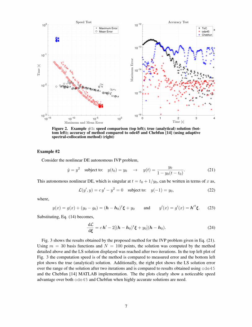
Fig. 2 shows the results obtained by the proposed method for the IVP problem given in Eq. (15).Using m = 60 basis functions and N = 200 points, the solution was computed by the methoddetailed above and the LS solution displayed was reached after two iterations. In the top left plot ofFig. 2 the computation speed is of the method is compared to measured error and the bottom leftplot shows the true (analytical) solution. Additionally, the right plot shows the LS solution errorover the range of the solution after two iterations and is compared to results obtained using ode45and the Chebfun [14] MATLAB implementation. The the plots clearly show a noticeable speedadvantage over both ode45 and Chebfun when highly accurate solutions are need.
6
10-15
10-10
10-5
100
10-3
10-2
10-1
100
Maximum Error
Mean Error
0 1 2 3 410
-16
10-15
10-14
10-13
10-12
ToC
ode45
Chebfun
Figure 2. Example #1: speed comparison (top left); true (analytical) solution (bot-tom left); accuracy of method compared to ode45 and Chebfun [14] (using adaptivespectral-collocation method) (right)
Example #2
Consider the nonlinear DE autonomous IVP problem,
y = y2 subject to: y(t0) = y0 → y(t) =y0
1− y0(t− t0). (21)
This autonomous nonlinear DE, which is singular at t = t0 + 1/y0, can be written in terms of x as,
L(y′, y) = c y′ − y2 = 0 subject to: y(−1) = y0, (22)
where,
y(x) = g(x) + (y0 − g0) = (h− h0)Tξ + y0 and y′(x) = g′(x) = h′
Tξ. (23)
Substituting, Eq. (14) becomes,
dLdξ
= ch′ − 2[(h− h0)Tξ + y0](h− h0). (24)
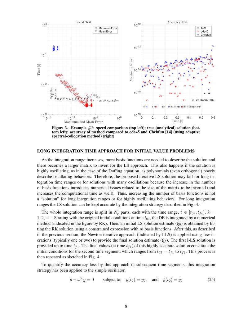
Fig. 3 shows the results obtained by the proposed method for the IVP problem given in Eq. (21).Using m = 30 basis functions and N = 100 points, the solution was computed by the methoddetailed above and the LS solution displayed was reached after two iterations. In the top left plot ofFig. 3 the computation speed is of the method is compared to measured error and the bottom leftplot shows the true (analytical) solution. Additionally, the right plot shows the LS solution errorover the range of the solution after two iterations and is compared to results obtained using ode45and the Chebfun [14] MATLAB implementation. The the plots clearly show a noticeable speedadvantage over both ode45 and Chebfun when highly accurate solutions are need.
7
10-15
10-10
10-5
100
10-3
10-2
10-1
100
Maximum Error
Mean Error
0 0.1 0.2 0.3 0.4 0.5 0.610
-16
10-15
10-14
10-13
10-12
ToC
ode45
Chebfun
Figure 3. Example #2: speed comparison (top left); true (analytical) solution (bot-tom left); accuracy of method compared to ode45 and Chebfun [14] (using adaptivespectral-collocation method) (right)
LONG INTEGRATION TIME APPROACH FOR INITIAL VALUE PROBLEMS
As the integration range increases, more basis functions are needed to describe the solution andthere becomes a larger matrix to invert for the LS approach. This also happens if the solution ishighly oscillating, as in the case of the Duffing equation, as polynomials (even orthogonal) poorlydescribe oscillating behaviors. Therefore, the proposed iterative LS solution may fail for long in-tegration time ranges or for solutions with many oscillations because the increase in the numberof basis functions introduces numerical issues related to the size of the matrix to be inverted (andincreases the computational time as well). Thus, increasing the number of basis functions is nota “solution” for long integration ranges or for highly oscillating behaviors. For long integrationranges the LS solution can be kept accurate by the integration strategy described in Fig. 4.
The whole integration range is split in Np parts, each with the time range, t ∈ [t0k, tfk], k =1, 2, · · · . Starting with the original initial conditions at time t01, the DE is integrated by a numericalmethod (indicated in the figure by RK). Then, an initial LS solution estimate (ξ0) is obtained by fit-ting the RK solution using a constrained expression with m basis functions. After this, as describedin the previous section, the Newton iterative approach (indicated by I-LS) is applied using few it-erations (typically one or two) to provide the final solution estimate (ξf ). The first I-LS solution isprovided up to time tf1. The final values (at time tf1) of this highly accurate solution constitute theinitial conditions for the second time segment, which ranges from t02 = tf1 to tf2. This process isthen repeated as sketched in Fig. 4.
To quantify the accuracy loss by this approach in subsequent time segments, this integrationstrategy has been applied to the simple oscillator,
y + ω2 y = 0 subject to: y(t0) = y0, and y(t0) = y0 (25)
8
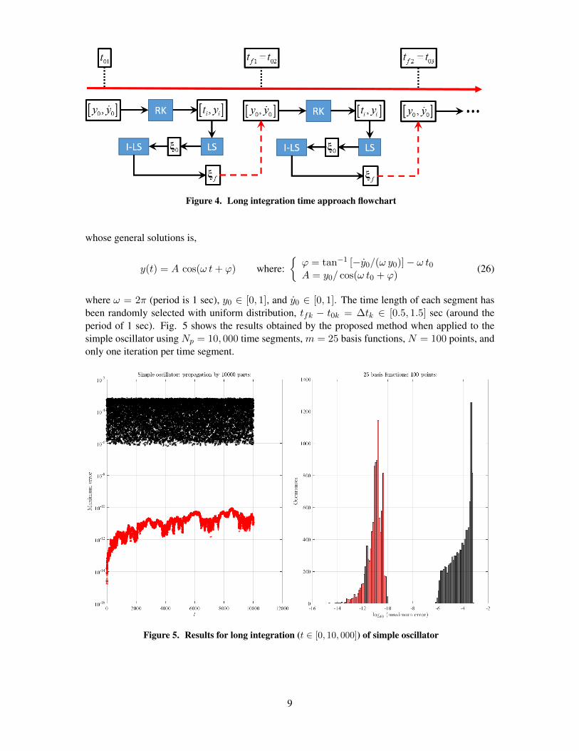
Figure 4. Long integration time approach flowchart
whose general solutions is,
y(t) = A cos(ω t+ ϕ) where:{ϕ = tan−1 [−y0/(ω y0)]− ω t0A = y0/ cos(ω t0 + ϕ)
(26)
where ω = 2π (period is 1 sec), y0 ∈ [0, 1], and y0 ∈ [0, 1]. The time length of each segment hasbeen randomly selected with uniform distribution, tfk − t0k = ∆tk ∈ [0.5, 1.5] sec (around theperiod of 1 sec). Fig. 5 shows the results obtained by the proposed method when applied to thesimple oscillator using Np = 10, 000 time segments, m = 25 basis functions, N = 100 points, andonly one iteration per time segment.
Figure 5. Results for long integration (t ∈ [0, 10, 000]) of simple oscillator
9
In the left plot of Fig. 5 the maximum absolute error experienced in each time segment (withrespect to the true values) is plotted for the LS (ξ0, with black marks) and the I-LS (ξf , with redmarks) solutions. The right plot of Fig. 5 shows the histograms of the logarithm in base 10 ofthese two maximum errors. These two plots are provided to show the upper bound of the true errorand to highlight that the accuracy loss during this process is limited. Actually, it seems that some“compensation” effect even occurs in some regions. This test shows that the error accuracy is stillbetter than 10−10 after 10, 000 integrations in consecutive ranges.
DUFFING EQUATION
The Duffing equation is an example of a dynamical system that exhibits chaotic behavior. TheDuffing equation is a nonlinear 2-nd order nonlinear DE used to model certain damped and drivenoscillators. The equation is,
y + δ y + α y + β y3 − γ cos(ω t) = 0 (27)
where, α controls the linear stiffness, β controls the amount of non-linearity in the restoring force,δ controls the amount of damping, γ is the amplitude of the periodic driving force, and ω is theangular frequency of the periodic driving force. In general, the Duffing equation does not admit anexact, analytic, solution. Therefore, a numerical method is used to obtain an approximate solution.
For numerical tests, let us assume the typical values adopted in the literature: α = −1, β = +1,δ = 0.3, ω = 1.2 and γ = 0.4 (usually, γ ∈ [0.2, 0.65]), with initial conditions y(t0) = y0 = 1 andy(t0) = y0 = 0. Using basis functions defined in x ∈ [−1,+1], the DE is written as,
L(y′′, y′, y, t) = c2y′′ + δ cy′ + α y + β y3 − γ cos(ω t) = 0, (28)
where t = t0 + (tf − t0)(x+ 1)/2 and where y is provided by the constrained expression
y(x) = g(x) + (y0− g0) + (x+ 1)
(y0c− g′0
)= (h−h0)
Tξ+ y0 + (x+ 1)
(y0c− h′0
Tξ
)(29)
and its derivatives,
y′ = (h′ − h′0)Tξ +y0c
and y′′ = h′′Tξ. (30)
The derivative in Eq. (14) are,
dLdξ
=∂L∂y′′·∂y′′
∂ξ+∂L∂y′·∂y′
∂ξ+∂L∂y·∂y∂ξ
= c2h′′+δ c(h′−h′0)+(α+3βy2)[h−h0−(x+1)h′0] (31)
Fig. 6 shows the results obtained by the proposed LS approach when applied to the Duffingoscillator. This figure shows the L2 norm of L(x, ξ) when fitting the ode45 (ξ = ξ0) solution andfor one and two iterations of the I-LS proposed approach (ξ1 and ξ2 solutions). In this example, byjust two iterations, 11 orders of magnitude accuracy gain is observed using m = 45 basis functionsand N = 100 points. Fig. 7 shows the results obtained when a long integration range is performedfor the Duffing oscillator as described by the flowchart shown in Fig. 4. The long integration rangeconsidered is Np = 10, 000 times the 4-sec time range considered in Fig. 6. The number of basisfunction and points per time segment adopted is the same as that adopted for a single 4-sec timesegment (m = 45 and N = 100 points). The left plot shows max(|Lk|) obtained when fitting theode45 solution (ξ0) and when using one and two iterations of the I-LS proposed approach (ξ1 andξ2 solutions). Again, we outline that the accuracy loss during this process is limited and the L2
norm of L(x, ξf ) obtained in the last range is still better than 10−10.
10
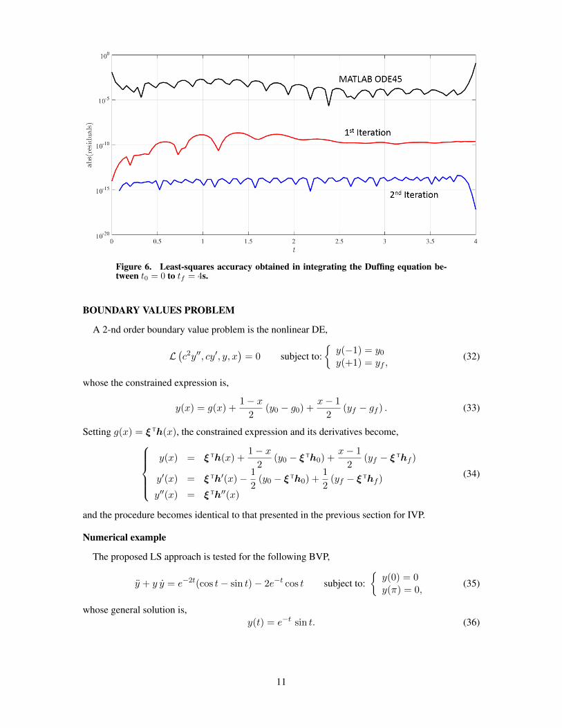
Figure 6. Least-squares accuracy obtained in integrating the Duffing equation be-tween t0 = 0 to tf = 4s.
BOUNDARY VALUES PROBLEM
A 2-nd order boundary value problem is the nonlinear DE,
L(c2y′′, cy′, y, x
)= 0 subject to:
{y(−1) = y0y(+1) = yf ,
(32)
whose the constrained expression is,
y(x) = g(x) +1− x
2(y0 − g0) +
x− 1
2(yf − gf ) . (33)
Setting g(x) = ξ Th(x), the constrained expression and its derivatives become,y(x) = ξ Th(x) +
1− x2
(y0 − ξ Th0) +x− 1
2(yf − ξ Thf )
y′(x) = ξ Th′(x)− 1
2(y0 − ξ Th0) +
1
2(yf − ξ Thf )
y′′(x) = ξ Th′′(x)
(34)
and the procedure becomes identical to that presented in the previous section for IVP.
Numerical example
The proposed LS approach is tested for the following BVP,
y + y y = e−2t(cos t− sin t)− 2e−t cos t subject to:{y(0) = 0y(π) = 0,
(35)
whose general solution is,y(t) = e−t sin t. (36)
11
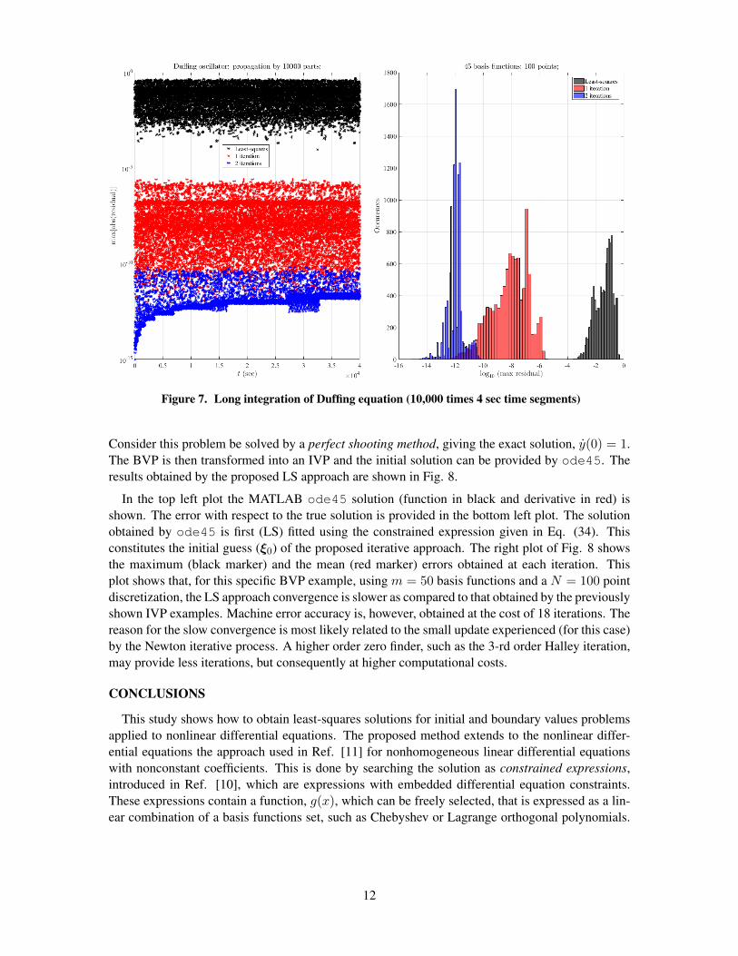
Figure 7. Long integration of Duffing equation (10,000 times 4 sec time segments)
Consider this problem be solved by a perfect shooting method, giving the exact solution, y(0) = 1.The BVP is then transformed into an IVP and the initial solution can be provided by ode45. Theresults obtained by the proposed LS approach are shown in Fig. 8.
In the top left plot the MATLAB ode45 solution (function in black and derivative in red) isshown. The error with respect to the true solution is provided in the bottom left plot. The solutionobtained by ode45 is first (LS) fitted using the constrained expression given in Eq. (34). Thisconstitutes the initial guess (ξ0) of the proposed iterative approach. The right plot of Fig. 8 showsthe maximum (black marker) and the mean (red marker) errors obtained at each iteration. Thisplot shows that, for this specific BVP example, using m = 50 basis functions and a N = 100 pointdiscretization, the LS approach convergence is slower as compared to that obtained by the previouslyshown IVP examples. Machine error accuracy is, however, obtained at the cost of 18 iterations. Thereason for the slow convergence is most likely related to the small update experienced (for this case)by the Newton iterative process. A higher order zero finder, such as the 3-rd order Halley iteration,may provide less iterations, but consequently at higher computational costs.
CONCLUSIONS
This study shows how to obtain least-squares solutions for initial and boundary values problemsapplied to nonlinear differential equations. The proposed method extends to the nonlinear differ-ential equations the approach used in Ref. [11] for nonhomogeneous linear differential equationswith nonconstant coefficients. This is done by searching the solution as constrained expressions,introduced in Ref. [10], which are expressions with embedded differential equation constraints.These expressions contain a function, g(x), which can be freely selected, that is expressed as a lin-ear combination of a basis functions set, such as Chebyshev or Lagrange orthogonal polynomials.
12
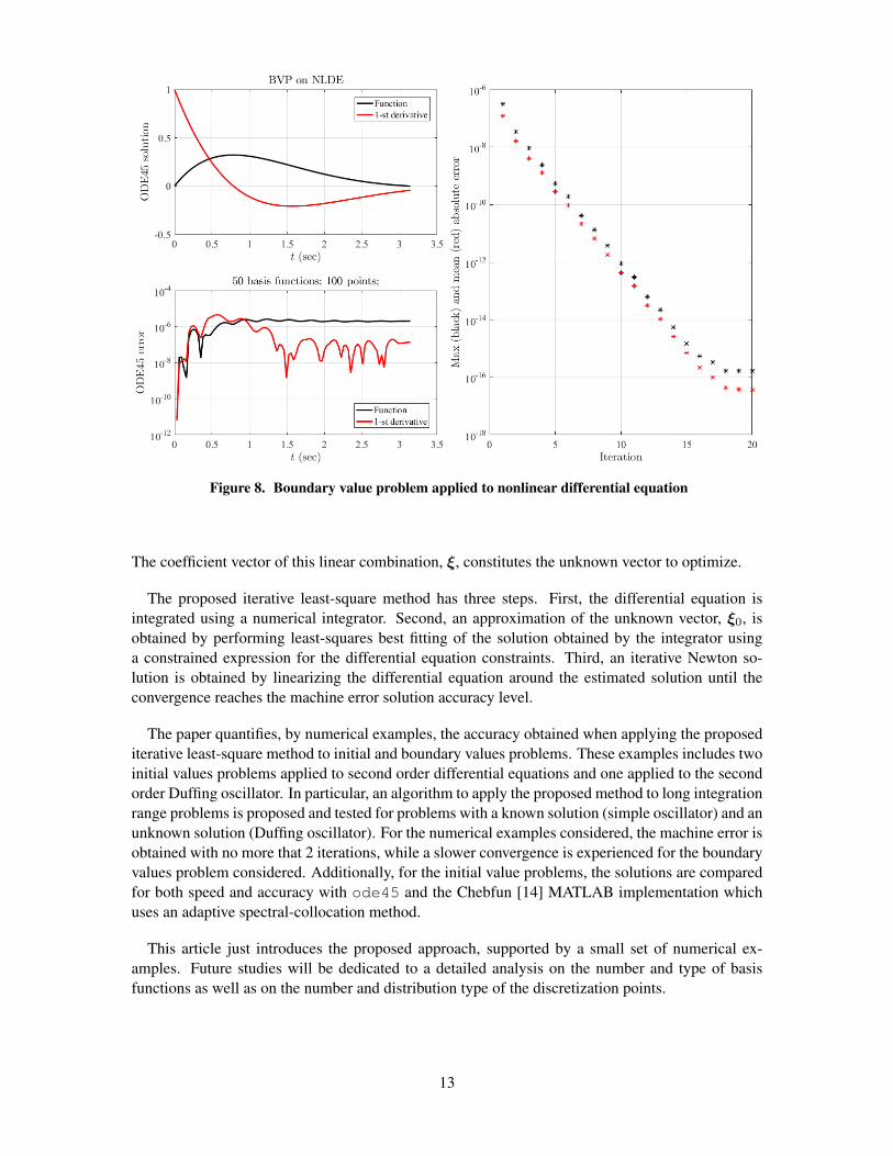
Figure 8. Boundary value problem applied to nonlinear differential equation
The coefficient vector of this linear combination, ξ, constitutes the unknown vector to optimize.
The proposed iterative least-square method has three steps. First, the differential equation isintegrated using a numerical integrator. Second, an approximation of the unknown vector, ξ0, isobtained by performing least-squares best fitting of the solution obtained by the integrator usinga constrained expression for the differential equation constraints. Third, an iterative Newton so-lution is obtained by linearizing the differential equation around the estimated solution until theconvergence reaches the machine error solution accuracy level.
The paper quantifies, by numerical examples, the accuracy obtained when applying the proposediterative least-square method to initial and boundary values problems. These examples includes twoinitial values problems applied to second order differential equations and one applied to the secondorder Duffing oscillator. In particular, an algorithm to apply the proposed method to long integrationrange problems is proposed and tested for problems with a known solution (simple oscillator) and anunknown solution (Duffing oscillator). For the numerical examples considered, the machine error isobtained with no more that 2 iterations, while a slower convergence is experienced for the boundaryvalues problem considered. Additionally, for the initial value problems, the solutions are comparedfor both speed and accuracy with ode45 and the Chebfun [14] MATLAB implementation whichuses an adaptive spectral-collocation method.
This article just introduces the proposed approach, supported by a small set of numerical ex-amples. Future studies will be dedicated to a detailed analysis on the number and type of basisfunctions as well as on the number and distribution type of the discretization points.
13

LINEAR LEAST-SQUARES METHODS
There are different numerical techniques to compute the linear least-squares (LS) solution ofA ξ = b. The most common methods are:
• The simplest approach consists with the (classic) solution,
ξ = (AT A)−1AT b. (37)
• using the QR decomposition,
A = QR → ξ = R−1QT b,
where Q is an orthogonal matrix and R an upper triangular matrix.
• using the SVD decompositions,
A = U ΣV T → ξ = A+ b = V Σ+ U T b
where U and V are two orthogonal matrices, and where Σ+ is the pseudo-inverse of Σ, whichis formed by replacing every non-zero diagonal entry by its reciprocal and transposing theresulting matrix.
• using the Cholesky decomposition,
ATA ξ = U TUξ = AT b → ξ = U−1(U−TAT b
)where U is a upper triangular and, consequently, U−1 and U−T are easy to compute.
Particular attention must be given to reduce the condition number by scaling. The correct methodof scaling is by scaling the columns of matrix A,
A(SS−1
)ξ = (AS)
(S−1ξ
)= Bη = b → ξ = S η = S (BTB)−1BTb (38)
where S is the m × m scaling diagonal matrix whose (diagonal) elements are the inverse of thenorms of the corresponding A matrix columns, skk = |ak|−1 or the maximum absolute value,skk = max
i|ak(i)|. The purpose of scaling is to decrease the condition number of the matrix to
invert.
In this article a scaled QR approach has been selected. This approach performs the QR decom-position of the scaled matrix,
B = AS = QR → ξ = S R−1QT b. (39)
A weighted LS solution can be obtained by introducing an n× n diagonal matrix of weights, W.This allows to increase the accuracy on time intervals of particular interest, as around initial or finaltimes,
W A ξ = W b → ξ = (AT W 2A)−1AT W b. (40)
Scaling the rows of matrix A is equivalent to perform weighted LS, as it can be easily proven.
14
BASIS FUNCTIONS
Since the proposed method uses a set of basis functions, a summary of the candidate orthogonalpolynomial basis functions is provided. Note that whatever basis functions type is adopted, constantand linear terms cannot be used because they have already been adopted to derive the constrainedexpressions for both IVP and BVP.
Chebyshev Orthogonal Polynomials
Chebyshev Orthogonal Polynomials of the first kind (COP), Tk(x), are defined in the x ∈[−1,+1] range and they are generated using the recursive function,
Tk+1 = 2xTk − Tk−1 starting from:
{T0 =1
T1 =x. (41)
All derivatives of COP can be computed in a recursive way, starting from
dT0dx
= 0,dT1dx
= 1 andddT0dxd
=ddT1dxd
= 0 (∀ d > 1), (42)
while the subsequent derivatives of Eq. (41) give for k ≥ 1,
dTk+1
dx= 2
(Tk + x
dTkdx
)− dTk−1
dx
d2Tk+1
dx2= 2
(2
dTkdx
+ xd2Tkdx2
)− d2Tk−1
dx2
......
...
ddTk+1
dxd= 2
(d
dd−1Tkdxd−1
+ xddTkdxd
)− ddTk−1
dxd; (∀ d ≥ 1).
(43)
In particular,
Tk(−1) = (−1)k,dTkdx
∣∣∣∣x=−1
= (−1)k+1 k2,d2Tkdx2
∣∣∣∣x=−1
= (−1)kk2 (k2 − 1)
3(44)
and
Tk(1) = 1,dTkdx
∣∣∣∣x=1
= k2,d2Tkdx2
∣∣∣∣x=1
=k2 (k2 − 1)
3. (45)
Legendre Orthogonal Polynomials
Legendre Orthogonal Polynomials (LeP), Lk(x), are defined in the x ∈ [−1,+1] range and theyare generated using the recursive function,
Lk+1 =2k + 1
k + 1xLk −
k
k + 1Lk−1 starting:
{L0 =1
L1 =x. (46)
All derivatives of LOP can be computed in a recursive way, starting from
dL0
dx= 0,
dL1
dx= 1 and
ddL0
dxd=
ddL1
dxd= 0 (∀ d > 1), (47)
15
while the subsequent derivatives of Eq. (46) for k ≥ 1, can be computed in cascade,
dLk+1
dx=
2k + 1
k + 1
(Lk + x
dLk
dx
)− k
k + 1
dLk−1dx
d2Lk+1
dx2=
2k + 1
k + 1
(2
dLk
dx+ x
d2Lk
dx2
)− k
k + 1
d2Lk−1dx2
......
...
ddLk+1
dxd=
2k + 1
k + 1
(d
dd−1Lk
dxd−1+ x
ddLk
dxd
)− k
k + 1
ddLk−1dxd
; (∀ d ≥ 1).
(48)
Laguerre Orthogonal Polynomials
Laguerre Orthogonal Polynomials (LaP), Lk(x), are generated using the recursive function,
Lk+1(x) =2k + 1− xk + 1
Lk(x)− k
k + 1Lk−1(x) starting:
{L0 =1
L1 =1− x. (49)
All derivatives of LOP can be computed in a recursive way, starting from
dL0
dx= 0,
dL1
dx= −1 and
ddL0
dxd=
ddL1
dxd= 0 (∀ d > 1),
thendLk+1
dx=
2k + 1− xk + 1
dLk
dx− 1
k + 1Lk −
k
k + 1
dLk−1dx
d2Lk+1
dx2=
2k + 1− xk + 1
d2Lk
dx2− 2
k + 1
dLk
dx− k
k + 1
d2Lk−1dx2
......
ddLk+1
dxd=
2k + 1− xk + 1
ddLk
dxd− d
k + 1
dd−1Lk
dxd−1− k
k + 1
ddLk−1dxd
(50)
Hermite Orthogonal Polynomials
There are two Hermite Orthogonal Polynomials (HOP), the probabilists, indicated by Ek(x) andthe physicists, indicated by Hk(x). They both are generated using the recursive function.
The probabilistists are defined as
Ek+1(x) = xEk(x)− kEk−1(x) starting:
{E0(x) =1
E1(x) =x(51)
All derivatives can be computed in a recursive way, starting from
dE0
dx= 0,
dE1
dx= 1 and
ddE0
dxd=
ddE1
dxd= 0 (∀ d > 1),
16

thendEk+1
dx= Ek + x
dEk
dx− k dEk−1
dx
d2Ek+1
dx2= 2
dEk
dx+ x
d2Ek
dx2− k d2Ek−1
dx2
......
ddEk+1
dxd= d
dd−1Ek
dxd−1+ x
ddEk
dxd− k ddEk−1
dxd
(52)
The physicists are defined as
Hk+1(x) = 2xHk(x)− 2kHk−1(x) starting:
{H0(x) =1
H1(x) =2x(53)
All derivatives can be computed in a recursive way, starting from
dH0
dx= 0,
dH1
dx= 2 and
ddH0
dxd=
ddH1
dxd= 0 (∀ d > 1),
thendHk+1
dx= 2Hk + 2x
dHk
dx− 2k
dHk−1dx
d2Hk+1
dx2= 4
dHk
dx+ 2x
d2Hk
dx2− 2k
d2Hk−1dx2
......
ddHk+1
dxd= 2d
dd−1Hk
dxd−1+ 2x
ddHk
dxd− 2k
ddHk−1dxd
(54)
Bessel Orthogonal Polynomials
Bessel Orthogonal Polynomials (BOP), Bk(x), are generated using the recursive function,
Bk+1(x) = (2k + 1)xBk(x) +Bk−1(x) starting:
{B0(x) = 1
B1(x) = 1 + x(55)
All derivatives of BOP can be computed in a recursive way, starting from
dB0
dx= 0,
dB1
dx= 1 and
ddB0
dxd=
ddB1
dxd= 0 (∀ d > 1),
thendBk+1
dx= (2k + 1)Bk + (2k + 1)x
dBk
dx+
dBk−1dx
d2Bk+1
dx2= 2(2k + 1)
dBk
dx+ (2k + 1)x
d2Bk
dx2+
d2Bk−1dx2
......
ddBk+1
dxd= d(2k + 1)
dd−1Bk
dxd−1+ (2k + 1)x
ddBk
dxd+
ddBk−1dxd
(56)
17
In addition, and for completeness, a Fourier basis functions is provided.
Fourier Basis
Fourier Series (FS) provides an approximation of the g(t) function
g(t) = a0 +
m∑k=1
[ak cos(kω0t) + bk sin(kω0t)] (57)
The first two derivatives of FS are
g(t) =m∑k=1
[−ak sin(kω0t) + bk cos(kω0t)] (kω0) (58)
and
g(t) =
m∑k=1
[−ak cos(kω0t)− bk sin(kω0t)] (kω0)2 (59)
where the basic frequency is selected as, ω0 =2π
tf − t0, that is one period for the [t0, tf ] time
interval.
REFERENCES[1] Dormand, J.R. and Prince, P.J. “A Family of Embedded Runge-Kutta Formulae,” Journal of Computa-
tional and Applied Mathematics, Vol. 6, 1980, pp. 19-26.[2] Berry, M.M. and Healy, L.M. “Implementation of Gauss-Jackson Integration for Orbit Propagation,”
The Journal of the Astronautical Sciences, Vol. 52, No. 3, 2004, pp. 331-357.[3] Elgohary T.A., Dong, L., Junkins, J.L., and Atluri, S.N. “Time Domain Inverse Problems in Nonlinear
Systems Using Collocation & Radial Basis Functions,” CMES: Computer Modeling in Engineering &Sciences, Vol. 100, No. 1, 2014, pp. 59-84.
[4] Elgohary, T.A., Junkins, J.L., and Atluri, S.N. “An RBF-Collocation Algorithm for Orbit Propagation,”Paper AAS 15-359 of the 2015 AAS/AIAA Space Flight Mechanics Meeting, Williamsburg, VA, Jan-uary 11-15, 2015.
[5] Bai, X., and Junkins, J.L. “Modified Chebyshev-Picard Iteration Methods for Orbit Propagation,” TheJournal of the Astronautical Sciences, Vol. 58, No. 4, 2011, pp. 583-613.
[6] Junkins, J.L., Bani Younes, A., Woollands, R., and Bai, X. “Picard Iteration, Chebyshev Polynomi-als, and Chebyshev Picard Methods: Application in Astrodynamics,” The Journal of the AstronauticalSciences, Vol. 60, No. 3, pp. 623-653, December 2015 (doi: 10.1007/s40295-015-0061-1).
[7] Reed J., Bani Younes A., Macomber B., Junkins, J.L. and Turner J. “State Transition Matrix for Per-turbed Orbital Motion using Modified Chebyshev Picard Iteration,” The Journal of the AstronauticalSciences, 2015, (doi: 10.1007/s40295-015-0051-3).
[8] Wright, K. “Chebyshev Collocation Methods for Ordinary Differential Equations,” The Computer Jour-nal 6.4 (1964), pp. 358-365.
[9] Gottlieb, D. and Orszag, S.A. “Numerical Analysis of Spectral Methods: Theory and Applications,”Society for Industrial and Applied Mathematics, 1977 (doi:10.1137/1.9781611970425).
[10] Mortari, D. “The Theory of Connections: Connecting Points,” Mathematics, 2017, 5, 57;doi:10.3390/math5040057.
[11] Mortari, D. “Least-squares Solutions of Linear Differential Equations,” Mathematics, 2017, 5, 48;doi:10.3390/math5040048.
[12] Strang, G. “Differential Equations and Linear Algebra,” Wellesley-Cambridge Press, 2015, ISBN0980232791, 9780980232790.
[13] Lin, Y., Enszer, J.A., and Stadtherr, M.A. “Enclosing all Solutions of Two-Point Boundary Value Prob-lems for ODEs,” Computers and Chemical Engineering, 2008, pp. 1714-1725.
[14] Platte, R.B. and Trefethen, L.N. “Chebfun: A New Kind of Numerical Computing,” Progress in Indus-trial Mathematics at ECMI, 2008, pp. 69-87.
18